


1. Introduction
The turbulent mixing of scalars, such as temperature, humidity, pollutants or any other chemical species, plays an important role in many engineering and scientific fields, including heat transfer, combustion, environmental pollution dispersion, oceanography and atmospheric science. Although many flows of interest contain more than one scalar (e.g. mixing of temperature and salinity in the ocean; mixing of temperature and humidity in the atmosphere; mixing of multiple reactants and products in combusting flows), there is a paucity of work on multi-scalar mixing. Moreover, previous studies on this subject have demonstrated limitations in some of the models commonly used in applications of multi-scalar mixing, and the few previous experimental studies that could be employed to either validate these models, or develop new ones are, in many ways, limited. For example, simultaneous measurements of multiple scalars are difficult to achieve, and a significant proportion of reported results consist only of scalar means, variances, covariances (or correlation coefficients), which may not be sufficient for the development or validation of new models. Furthermore, most studies of multi-scalar mixing have only focused on scalar fields despite the fact that simultaneous velocity-scalar measurements are required to fully describe turbulent scalar mixing. (A notable exception is the experiments of Sirivat & Warhaft Reference Sirivat and Warhaft1982.)
To this end, the overall objective of the present work will be to expand our understanding of multi-scalar mixing by providing valuable new experimental data, specifically addressing the current lack of simultaneous multi-scalar and velocity measurements in the literature. We have developed an experimental technique capable of simultaneously measuring two scalars (helium concentration and temperature) and velocity in turbulent flows and apply it herein to study the evolution of multiple scalars in turbulent coaxial jets emanating into a coflow. Of particular interest is the effect that the momentum flux ratio of the coaxial jets has on mixing within this flow.
The remainder of this work is organized as follows. Reviews of the subject of multi-scalar mixing and the dynamics of coaxial jets are presented in § 2. The experimental apparatus and conditions are respectively described in § 3 and § 4. Results are then examined in § 5. Finally, concluding remarks are provided in § 6.
2. Literature review
2.1. Multi-scalar mixing
Early studies of multi-scalar mixing were performed with a measurement technique known as the inference method, in which the covariance of two identical scalar sources (usually two thermal sources) was inferred from measurements of both scalar sources operating simultaneously along with those of each scalar source operating alone, such that
 \begin{equation} \langle \phi_{\alpha}'\phi_{\beta}' \rangle=\tfrac{1}{2} \Big[\langle(\phi_{\alpha}'+\phi_{\beta}')^2\rangle-\langle \phi_{\alpha}'^2\rangle-\langle\phi_{\beta}'^2\rangle\Big], \end{equation}
where  $\phi _{\alpha }'$ and $\phi _{\beta }'$ represent fluctuations in the two respective scalars, and $\langle \phi_{\alpha}'\phi_{\beta}' \rangle$ is their covariance. (As in Pope (Reference Pope2000), the scalar field is defined as $\phi =\langle \phi \rangle +\phi '$, where $\phi '$ denotes the scalar fluctuations; similarly, the axial velocity is defined as $U=\langle U \rangle +u$.) In such studies, mixing was typically quantified using the scalar cross-correlation coefficient ( $\rho _{\phi _{\alpha }\phi _{\beta }}$):
 \begin{equation} \rho_{\phi_{\alpha}\phi_{\beta}} = \frac{\langle \phi_{\alpha}' \phi_{\beta}' \rangle}{\langle \phi_{\alpha}'^2\rangle^{1/2} \langle \phi_{\beta}'^2 \rangle^{1/2}}, \end{equation}
which is a non-dimensionalized form of the aforementioned scalar covariance.
Using the inference technique, Warhaft (Reference Warhaft1981) first showed that the cross-correlation coefficient (and the covariance) from two longitudinally separated arrays of fine heated wires (mandolines) in grid turbulence decreased with increasing downstream distance, such that initially positively correlated scalars became progressively less correlated. Sirivat & Warhaft (Reference Sirivat and Warhaft1982) went on to clarify that for the same flow there existed certain situations in which the scalar cross-correlation coefficient (but not the covariance) would remain constant, or even increase in the downstream direction. Subsequently, Warhaft (Reference Warhaft1984) demonstrated that the evolution of the scalar cross-correlation coefficient of two (or more) laterally separated line sources was strongly dependent on the initial flow conditions, including the source location and spacing.
The evolution of the scalar cross-correlation of two laterally separated sources in a turbulent flow may generally be described as follows. (i) Initially this correlation coefficient is undefined, as the measurement probe is rarely exposed to either of the plumes produced by the scalar sources. (ii) Farther downstream, the initially ‘thin’ scalar plumes begin to meander and ‘flap’ in sync with one another due to the motions of the largest eddies in the flow, and the measurement probe begins to alternatively sample each plume, but not both at the same time, so that the correlation coefficient becomes increasingly negative. (iii) The scalar plumes then begin to overlap and mix, and the correlation coefficient starts to increase, eventually becoming positive. (iv) The cross-correlation coefficient finally tends towards an asymptotic value of 1 (Warhaft Reference Warhaft1984; Sawford, Frost & Allan Reference Sawford, Frost and Allan1985; Tong & Warhaft Reference Tong and Warhaft1995; Davies et al. Reference Davies, Jones, Manning and Thomson2000; Vrieling & Nieuwstadt Reference Vrieling and Nieuwstadt2003; Costa-Patry & Mydlarski Reference Costa-Patry and Mydlarski2008; Oskouie, Wang & Yee Reference Oskouie, Wang and Yee2015, Reference Oskouie, Wang and Yee2017; Oskouie, Yang & Wang Reference Oskouie, Yang and Wang2018). It was additionally found that the scalar cross-correlation coefficient evolves faster towards its asymptotic state as the source separation decreases (Costa-Patry & Mydlarski Reference Costa-Patry and Mydlarski2008; Oskouie et al. Reference Oskouie, Wang and Yee2015, Reference Oskouie, Wang and Yee2017, Reference Oskouie, Yang and Wang2018).
Although the scalar cross-correlation coefficient can provide valuable quantitative information about mixing within the flow, it may not always fully capture that mixing (Li et al. Reference Li, Yuan, Carter and Tong2017). One of the disadvantages of the inference method, which has been used in most previous experimental studies of multi-scalar mixing (e.g. Warhaft Reference Warhaft1984; Tong & Warhaft Reference Tong and Warhaft1995; Costa-Patry & Mydlarski Reference Costa-Patry and Mydlarski2008), is that simultaneous measurements of both scalar quantities is not possible. Although covariances and correlation coefficients, as well as co- and coherency spectra, for two scalar sources can be obtained using this method, important statistics, such as the scalar–scalar joint probability density function (JPDF), cannot be measured by way of this method. This quantity is of particular interest, given that PDF methods, which involve solving a modelled transport equation for the one-point, one-time Eulerian scalar–scalar JPDF ( $\,f_{\phi _{\alpha }\phi _{\beta }}$)
 \begin{align}
& \frac{\partial f_{\phi_{\alpha}\phi_{\beta}}}{\partial t}+
\frac{\partial}{\partial
x_j}\Big[f_{\phi_{\alpha}\phi_{\beta}}(\langle U_j \rangle
+ \langle u_j \rvert \hat{\phi_{\alpha}},
\hat{\phi_{\beta}} \rangle) \Big] \nonumber\\ &\quad
={-}\frac{\partial}{\partial
\hat{\phi_{\alpha}}}\Big(f_{\phi_{\alpha}\phi_{\beta}}
[\langle \gamma_{\alpha} \nabla^2\phi_{\alpha}
\rvert \hat{\phi_{\alpha}}, \hat{\phi_{\beta}}
\rangle+S_{\phi_{\alpha}}( \hat{\phi_{\alpha}},
\hat{\phi_{\beta}})]\Big) \nonumber\\ &\qquad
-\frac{\partial}{\partial
\hat{\phi_{\beta}}}\Big(f_{\phi_{\alpha}\phi_{\beta}}
[\langle \gamma_{\beta} \nabla^2\phi_{\beta}
\rvert \hat{\phi_{\alpha}}, \hat{\phi_{\beta}}
\rangle+S_{\phi_{\beta}}( \hat{\phi_{\alpha}},
\hat{\phi_{\beta}})]\Big),
\end{align}
\begin{align}
& \frac{\partial f_{\phi_{\alpha}\phi_{\beta}}}{\partial t}+
\frac{\partial}{\partial
x_j}\Big[f_{\phi_{\alpha}\phi_{\beta}}(\langle U_j \rangle
+ \langle u_j \rvert \hat{\phi_{\alpha}},
\hat{\phi_{\beta}} \rangle) \Big] \nonumber\\ &\quad
={-}\frac{\partial}{\partial
\hat{\phi_{\alpha}}}\Big(f_{\phi_{\alpha}\phi_{\beta}}
[\langle \gamma_{\alpha} \nabla^2\phi_{\alpha}
\rvert \hat{\phi_{\alpha}}, \hat{\phi_{\beta}}
\rangle+S_{\phi_{\alpha}}( \hat{\phi_{\alpha}},
\hat{\phi_{\beta}})]\Big) \nonumber\\ &\qquad
-\frac{\partial}{\partial
\hat{\phi_{\beta}}}\Big(f_{\phi_{\alpha}\phi_{\beta}}
[\langle \gamma_{\beta} \nabla^2\phi_{\beta}
\rvert \hat{\phi_{\alpha}}, \hat{\phi_{\beta}}
\rangle+S_{\phi_{\beta}}( \hat{\phi_{\alpha}},
\hat{\phi_{\beta}})]\Big),
\end{align}
are frequently used in applications involving the transport of multiple scalars. (Note that  $U$,
$U$,  $u$,
$u$,  $\gamma$ and $S_{\phi }$ respectively denote the instantaneous and fluctuating velocity, scalar diffusivity and scalar addition due to chemical reaction.)
Scalar–scalar JPDFs were first reported in homogeneous isotropic turbulence and three-stream scalar mixing layers using direct numerical simulations (DNS) (Juneja & Pope Reference Juneja and Pope1996; Sawford & de Bruyn Kops Reference Sawford and de Bruyn Kops2008). More recently, experimental techniques enabling simultaneous multi-scalar measurements – such as two-channel laser-induced fluorescence (LIF) (Saylor & Sreenivasan Reference Saylor and Sreenivasan1998; Lavertu, Mydlarski & Gaskin Reference Lavertu, Mydlarski and Gaskin2008; Soltys & Crimaldi Reference Soltys and Crimaldi2011, Reference Soltys and Crimaldi2015; Shoaei & Crimaldi Reference Shoaei and Crimaldi2017) or planar laser-induced fluorescence (PLIF) and planar laser Rayleigh scattering (Cai et al. Reference Cai, Dinger, Li, Carter, Ryan and Tong2011; Li et al. Reference Li, Yuan, Carter and Tong2017, Reference Li, Yuan, Carter and Tong2021) – then made it possible to measure scalar–scalar JPDFs in both parallel and coaxial jets in a coflow (Cai et al. Reference Cai, Dinger, Li, Carter, Ryan and Tong2011; Soltys & Crimaldi Reference Soltys and Crimaldi2015; Li et al. Reference Li, Yuan, Carter and Tong2017). These authors additionally measured the conditional scalar diffusion ( $\langle \gamma _{\alpha } \nabla ^2 \phi _{\alpha } \rvert \hat {\phi _{\alpha }}, \hat {\phi _{\beta }} \rangle$, $\langle \gamma _{\beta } \nabla ^2 \phi _{\beta } \rvert \hat {\phi _{\alpha }}, \hat {\phi _{\beta }} \rangle$), which is said to ‘transport’ the scalar–scalar JPDF in scalar space, and appears in unclosed form in (2.3) (Cai et al. Reference Cai, Dinger, Li, Carter, Ryan and Tong2011). It was observed that this term quickly converged along a manifold (or mixing path), which had to make a detour in scalar space, because the scalars were initially separated. This has important implications, since it presents difficulties for existing mixing models used to account for the effects of molecular diffusion in PDF methods. (Examples of such models include the interaction by exchange with the mean (IEM) model, modified curl (MC) model, Euclidean minimum spanning tree (EMST) model and interaction by exchange with the conditional mean (IECM) model. (See Curl Reference Curl1963; Villermaux & Devillon Reference Villermaux and Devillon1972; Dopazo & O'Brien Reference Dopazo and O'Brien1974; Janicka, Kolbe & Kollmann Reference Janicka, Kolbe and Kollmann1979; Pope Reference Pope1994, Reference Pope1998; Subramaniam & Pope Reference Subramaniam and Pope1998).) As discussed by Cai et al. (Reference Cai, Dinger, Li, Carter, Ryan and Tong2011), many of these models do not take into account the spatial (i.e. physical-space) structure of the scalars, and accordingly may not be suitable for extension to multi-scalar mixing.
A number of other studies have further examined the accuracy of such models when it comes to reproducing the mixing of multiple scalars (Sawford Reference Sawford2004; Sawford & de Bruyn Kops Reference Sawford and de Bruyn Kops2008; Viswanathan & Pope Reference Viswanathan and Pope2008; Meyer & Deb Reference Meyer and Deb2012; Rowinski & Pope Reference Rowinski and Pope2013). The IECM model (including modified forms) was shown to have good agreement with experimental data (i.e. variances and correlation coefficients) obtained by Warhaft (Reference Warhaft1984) in homogeneous, isotropic turbulence (Sawford Reference Sawford2004; Viswanathan & Pope Reference Viswanathan and Pope2008). In three-stream scalar mixing layers, Sawford & de Bruyn Kops (Reference Sawford and de Bruyn Kops2008) similarly demonstrated that this model agrees well with DNS of scalar cross-correlation coefficients. Additionally, Rowinski & Pope (Reference Rowinski and Pope2013) found that Reynolds-averaged Navier–Stokes (RANS) PDF calculations with the IEM, MC, EMST models were capable of reproducing the low-order statistical moments (e.g. scalar means and variances) measured by Cai et al. (Reference Cai, Dinger, Li, Carter, Ryan and Tong2011) in coaxial jets. However, many mixing models, including the IECM, IEM, MC, EMST models, have shown poor agreement with scalar–scalar JPDFs and conditional mean velocities reported in previous studies (Sawford & de Bruyn Kops Reference Sawford and de Bruyn Kops2008; Meyer & Deb Reference Meyer and Deb2012; Rowinski & Pope Reference Rowinski and Pope2013). Consequently, although these models can reconstruct certain scalar interactions, they do not reproduce them all with sufficient accuracy. It is for this reason that new experimental data, particularly those obtained by simultaneous multi-scalar and velocity measurements, are needed to better understand the limitations of current mixing models and/or develop new ones.
2.2. Coaxial jets
As noted previously, the present work focuses on multi-scalar mixing in coaxial jets. As such, it is beneficial to describe these jets in greater detail. Coaxial jets, which consist of an (inner) centre and (outer) annular jet, have numerous practical engineering applications, and are frequently used to mix multiple fluid streams together. Their evolution depends on a variety of factors, including the inner ( $U_1$) and outer ( $U_2$) jet velocities, the inner ( $\rho _1$) and outer ( $\rho _2$) jet densities, the geometry at the exit of the jets (characterized by the inner and outer diameters, $D_1$ and $D_2$, as well as the wall separating the two jet streams), the characteristics of the velocity profiles at the jet exit and the level of free-stream turbulence (Rehab, Villermaux & Hopfinger Reference Rehab, Villermaux and Hopfinger1997; Buresti, Petagna & Talamelli Reference Buresti, Petagna and Talamelli1998; Sadr & Klewicki Reference Sadr and Klewicki2003; Segalini & Talamelli Reference Segalini and Talamelli2011). Nevertheless, the flow in such jets, which is illustrated in figure 1, can generally be described as follows.
A schematic representation of two coaxial jets, where the inner and outer jets respectively consist of scalar  $\phi _1$ and $\phi _2$, and issue into surroundings of $\phi _3$ (which may be either a slow coflow, as is the case in the present work, or quiescent). The three zones of flow defined by Ko & Kwan (Reference Ko and Kwan1976) are listed on the left. The potential core of the inner and outer jets, as well as the inner and outer mixing regions are noted on the right.

Close to the jet exits, coaxial jets exhibit two potential cores – for the inner and outer jets, respectively – separated by an inner mixing region in which the centre and annular jets mix with each other, but not the ambient fluid. The potential core of the annular jet (i.e. the outer core) is surrounded by an outer mixing region in which the annular jet and ambient fluid mix. Farther downstream, the cores disappear, and the coaxial jets behave like a single jet and exhibit self-similarity (Champagne & Wygnanski Reference Champagne and Wygnanski1971). Ko and co-authors (Ko & Kwan Reference Ko and Kwan1976; Ko & Au Reference Ko and Au1981, Reference Ko and Au1985; Au & Ko Reference Au and Ko1987) have suggested that the flow be described in terms of three zones: (i) an initial merging zone, containing the inner and outer cores, (ii) an intermediate merging zone beyond the end of the outer core in which the inner and outer mixing regions mix and (iii) a fully merged zone, in which the centre (inner) and annular (outer) jets have merged. For jets in which the velocity ratio ( $R=U_2/U_1$) is greater than one, the intermediate merging zone is said to end at the downstream distance at which the maximum velocity intercepts the centreline – a location referred to as the reattachment point, since it marks the point where the outer mixing regions reach the centreline and ‘reattach’ (Ko & Au Reference Ko and Au1985).
As summarized in table 1, most studies of coaxial jets have focused on the velocity field of constant-density jets. In those studies, significant attention has been paid to the effect of the velocity ratio of the two jets ( $R=U_2/U_1$) on the flow. In general, the velocity ratio has been shown to have a minor effect on the length of the outer potential core or the reattachment point (Champagne & Wygnanski Reference Champagne and Wygnanski1971; Ko & Au Reference Ko and Au1981, Reference Ko and Au1982, Reference Ko and Au1985; Buresti et al. Reference Buresti, Petagna and Talamelli1998; Warda et al. Reference Warda, Kassab, Elshorbagy and Elsaadawy1999). Thus, the three zones described by Ko & Kwan (Reference Ko and Kwan1976) appear to be nearly independent of $R$. However, the length of the inner potential core is strongly dependent on the velocity ratio (Champagne & Wygnanski Reference Champagne and Wygnanski1971; Ko & Kwan Reference Ko and Kwan1976; Ko & Au Reference Ko and Au1981; Rehab et al. Reference Rehab, Villermaux and Hopfinger1997; Warda et al. Reference Warda, Kassab, Elshorbagy and Elsaadawy1999). For example, in coaxial jets in which $1< R< R_{cr}$ (where $R_{cr}$ is a critical velocity ratio beyond which appears a separate flow regime characterized by an unsteady re-circulation bubble Rehab et al. Reference Rehab, Villermaux and Hopfinger1997; Balarac & Métais Reference Balarac and Métais2005), Rehab et al. (Reference Rehab, Villermaux and Hopfinger1997) demonstrated that the length of the inner potential core varied as ${\sim }R^{-1}$. For small to moderate velocity ratios ( $R< R_{cr}$), increasing the velocity ratio has been associated with higher turbulence intensities and faster development of the two jets (Champagne & Wygnanski Reference Champagne and Wygnanski1971; Buresti et al. Reference Buresti, Petagna and Talamelli1998), leading both Champagne & Wygnanski (Reference Champagne and Wygnanski1971) and Warda et al. (Reference Warda, Kassab, Elshorbagy and Elsaadawy1999) to conclude that $R$ should be greater than 1 to enhance mixing between the two jets. In coaxial jets in which the initial densities of the respective jet stream differ – which is the case in many practical applications – it was suggested that the effects of density can be incorporated into the momentum flux ratio ( $M$)
$M$)
 \begin{equation} M=SR^2, \end{equation}
where  $S$ (
$S$ ( $=\rho _2/\rho _1$) is the density ratio of the outer and inner jets. In such jets, values for the lengths of the inner potential core, as well as $M_{cr}$ (where $M_{cr}=SR_{cr}^2$), are consistent with those observed in constant-density jets (Favre-Marinet et al. Reference Favre-Marinet, Camano and Sarboch1999; Favre-Marinet & Schettini Reference Favre-Marinet and Schettini2001; Schumaker & Driscoll Reference Schumaker and Driscoll2012). Accordingly, it is $M$ rather than $R$ which should be used to describe the behaviour of (constant- and variable-density) coaxial jets.
Summary of studies of axisymmetric coaxial jets in which velocity and scalar field data are reported. The experimental and numerical methods used within the works are: hot-wire anemometry (HWA), laser doppler anemometry (LDA), PLIF, LIF, molecular tagging velocimetry (MTV), Rayleigh scattering (RS), marker nephelometry (MN) and DNS. Where available, the velocity ( $U_2/U_1$), density ( $\rho _2/\rho _1$), diameter ( $D_2/D_1$) and area ( $A_2/A_1$) ratios of the two coaxial jets are provided, as is the thickness of the wall separating them ( $t$).
$t$).

Nevertheless, given that most studies of coaxial jets have involved constant-density jets, these have examined the effects of  $R$ rather than those of $M$. A more complex description of these jets was given by Segalini & Talamelli (Reference Segalini and Talamelli2011), who suggested that there exist important differences between the dynamics of jets with different velocity ratios. Specifically, when $R<0.75$, instabilities in the inner and outer shear layers of the jets develop independently and the flow dynamics is driven by the inner shear layer. When $R \approx 1$, the jet dynamics is driven by vortex shedding from the separating wall. And when $R>1.6$ (and $R< R_{cr}$), the outer shear layer imposes its dynamics on the inner shear layer, creating a ‘lock-in’ phenomenon. Similarly, Dahm, Frieler & Tryggvason (Reference Dahm, Frieler and Tryggvason1992) noted that in addition to the velocity jump that results from the difference in jet velocities, there is also a velocity defect created by the viscous boundary layers on either side of the wall separating the two jet streams, which must be considered. Using flow visualizations, they furthermore demonstrated that the dynamics of the flow depended on both the velocity ratio and the absolute velocities of the jets. Other researchers have found that the geometry of coaxial jets (i.e. jet diameters, wall thickness) affects the lengths of the inner and outer potential cores, as well as interpenetration of the jet streams, further underscoring the importance that initial conditions have on their development (Au & Ko Reference Au and Ko1987; Rehab et al. Reference Rehab, Villermaux and Hopfinger1998; Talamelli et al. Reference Talamelli, Segalini, Örlü and Buresti2013).
Fewer studies have examined the scalar fields of coaxial jets, especially those which transport multiple scalars. In such studies, it has been important to understand how mixing of all scalars progresses throughout the jets. Grandmaison et al. (Reference Grandmaison, Becker and Zettler1996), Cai et al. (Reference Cai, Dinger, Li, Carter, Ryan and Tong2011) and Li et al. (Reference Li, Yuan, Carter and Tong2017) each studied the mixing of scalars respectively released from the centre and annular jets, and observed that – in contrast to the more commonly studied case of two laterally separated scalars (described in § 2.1) – the scalar cross-correlation coefficient along the axis of the jets increased from an initial value of  $-1$ to $1$. Given that the two scalars are initially side by side, and not separated by ambient fluid, both the mixing process and the conditions that affect it are distinct from those that have been described in previous studies of multi-scalar mixing. Both Grandmaison et al. (Reference Grandmaison, Becker and Zettler1996) and Li et al. (Reference Li, Yuan, Carter and Tong2017) noted that in their constant-density coaxial jets the evolution of this parameter, as well as mixing in general, depended on the velocity ratio ( $R$). The latter indicated that increasing $R$ lead to increased turbulent transport, such that the scalar evolution was initially faster, but decreased small-scale mixing, such that the scalar evolution was delayed downstream. However, it is important to note that the work of Grandmaison et al. (Reference Grandmaison, Becker and Zettler1996) was restricted to coaxial jets in which $R>1$, and does not involve simultaneous measurements of two scalars, whereas that of Li et al. (Reference Li, Yuan, Carter and Tong2017) only considers two different velocity ratios, both of which are less than 1. Moreover, neither report velocity measurements, despite the fact that the velocity ratio directly affects the velocity field of coaxial jets. Using simultaneous multi-scalar and velocity measurements, the present work clarifies the effect that this important parameter – expressed more generally as the momentum flux ratio – has on scalar mixing within the flow. To explore any differences that may exist between the dynamics of jets in which $M<1$ or those in which $M>1$, momentum flux ratios ranging from 0.77 to 4.2 are investigated in the present work.
3. Experimental apparatus
3.1. Flow facility
The experiments herein were carried out in the coaxial jet apparatus depicted in figure 2. A detailed description of the entire flow facility, including the coaxial jet apparatus and equipment employed to calibrate measurement probes, is given in Hewes (Reference Hewes2021). As the calibration equipment is also described in Hewes & Mydlarski (Reference Hewes and Mydlarski2021a,Reference Hewes and Mydlarskib), only the details of the coaxial jet apparatus are summarized herein.
Schematic of the coaxial jet apparatus and 3-wire thermal-anemometry-based probe.

The coaxial jet apparatus is housed in a large  $1.8\,{\rm m} \times 1.7\,{\rm m}\times 2.4\,{\rm m}$ enclosure, which shields it from external flow perturbations. As may be observed in figure 2, it consists of (i) a centre jet containing an (unheated) mixture of helium and air, (ii) an annular jet containing pure (unheated) air and (iii) a coflow containing (pure) heated air. The He/air mixtures supplied to the centre jet are produced far upstream by joining a continuous stream of helium with a continuous stream of air. The flow rate of the air stream, and ultimately, the total flow rate of the mixture, is set using a needle valve. Helium concentrations are controlled by means of a 100 slpm mass flow meter (Alicat M-100SLPM-D) and a 20 slpm mass flow controller (Alicat MC-20SLPM-D); the former measures the flow rate of the air stream and the latter uses an automated, custom-made LabVIEW program to set the flow rate of the helium stream to provide the desired helium concentration. The air supplied to the coflow is heated upstream in a long copper cylinder to which three 80 $\varOmega$ strip heaters are attached. The flow rate of this air stream, along with that supplied to the annular jet, is controlled using a 500 slpm mass flow controller (Alicat M-500SLPM-D). The coaxial jet apparatus was constructed such that the ratio of the annular and centre jet diameters ( $D_2/D_1$) is 2.1 and the thickness of the wall separating these jets ( $t$) is 1.6 mm. Additional dimensions and properties are provided in table 2. Three Velmex BiSlide traversing mechanisms were mounted sufficiently far from the coaxial jets to not interfere with the flow and used to support and translate the measurement probes described in the following subsection.
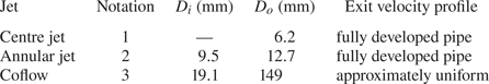
Properties of the coaxial jet apparatus. The inner ( $D_i$) and outer ( $D_o$) diameters of the tubes used to produce each jet, as well as their exit velocity profile are provided. Note that henceforth the centre jet, annular jet and coflow are respectively referred to with the subscripts 1, 2 and 3.
3.2. Instrumentation
Measurements were performed using a 3-wire thermal-anemometry-based probe, like that described in Hewes & Mydlarski (Reference Hewes and Mydlarski2021b). It is capable of simultaneously measuring velocity, helium concentration and temperature in turbulent flows. As depicted in figure 2, this probe is composed of (i) an interference probe, which is used to measure velocity and helium concentration, and (ii) a cold-wire thermometer, which is used to measure temperature.
The interference probe herein is constructed from two tungsten hot-wires, placed approximately 10  $\mathrm {\mu }$m apart. The upstream wire of the probe is 5 $\mathrm {\mu }$m in diameter, 1.2 mm long and maintained at an overheat ratio of 1.8, whereas the downstream one is 2.5 $\mathrm {\mu }$m in diameter, 0.2 mm long and maintained at an overheat ratio of 1.2. In this configuration, the behaviour of the downstream wire is strongly influenced by the thermal field of the upstream wire, and responds differently to changes in the flow's velocity or concentration. As explained in Hewes & Mydlarski (Reference Hewes and Mydlarski2021a), this makes it possible to simultaneously measure the aforementioned quantities in isothermal flows. The cold-wire thermometer is placed approximately 1 mm away from the interference probe, and consists of a 0.63 $\mathrm {\mu }$m diameter platinum wire with a length-to-diameter ratio ( $l/d$) of approximately 800. As noted in Mydlarski & Warhaft (Reference Mydlarski and Warhaft1998) and other works (e.g. Lavertu & Mydlarski Reference Lavertu and Mydlarski2005), the chosen value of $l/d$ represents a compromise between the desired spatial resolution and length required to minimize conduction between the cold-wire and its prongs.
Given that the 3-wire probe is used to measure velocity, helium concentration and temperature in non-isothermal turbulent flows of varying concentration, it is important to discuss the effects of (i) temperature on the interference probe and (ii) velocity and concentration on the cold-wire thermometer. Although the interference probe is sensitive to the temperature field of the flow, the cold-wire can be assumed to be effectively insensitive to the velocity and concentration fields. (The former is well established and discussed in Bruun (Reference Bruun1995), whereas the latter is demonstrated in Hewes & Mydlarski Reference Hewes and Mydlarski2021b.) Thus, temperature may be measured independently of both velocity and helium concentration, and the cold-wire can be employed to compensate for the effects of temperature fluctuations on the interference probe. A method to do so is described in detail in Hewes & Mydlarski (Reference Hewes and Mydlarski2021b).
The interference probe and cold-wire were calibrated separately in the calibration apparatus mentioned in § 3.1, which generates laminar flows of different, known velocities, helium concentrations and temperatures. They were then combined to form the 3-wire probe. After finishing all experiments, a calibration for the interference probe was repeated to account for any possible drift, which in thermal-anemometry techniques may arise from a variety of factors, including changes in ambient temperature, humidity and probe resistance (Hewes et al. Reference Hewes, Medvescek, Mydlarski and Baliga2020). Additional information on the calibration procedures may be found in Hewes & Mydlarski (Reference Hewes and Mydlarski2021a,Reference Hewes and Mydlarskib). Data acquisition and post-processing methods for the 3-wire probe are explained in the following section.
3.3. Data acquisition and post-processing
The two wires comprising the interference probe were operated using two channels of a TSI IFA300 constant temperature anemometer, and the cold-wire thermometer was operated using a custom-made constant current anemometer which was built at the Université Laval in Québec, Canada (see Lemay & Benaïssa Reference Lemay and Benaïssa2001). Fluctuating signals from all three wires were band-pass filtered using Krohn-Hite 3382 and 3384 filters to remove frequencies above the Kolmogorov and Corrsin scales. (Mean quantities were only low-pass filtered.) The signals were then digitized using a 16-bit National Instrument PCI-6143 data acquisition board. Time series of the data were obtained by simultaneously sampling each wire at twice the low-pass frequency (as specified by the Nyquist criterion) for approximately 5–10 min (long enough that the statistics reported herein are converged; Hewes Reference Hewes2021).
The fluid temperature ( $T$) was calculated as follows:
 \begin{equation} T=A_c+B_cE_c, \end{equation}
using the output voltage of the cold-wire thermometer ( $E_c$). As discussed above, the cold-wire was used to compensate for temperature effects on the interference probe, yielding signals for the upstream and downstream wire of this probe that are normalized to be temperature independent ( $E_{up, n}$ and $E_{down, n}$, respectively). The helium concentration ( $C$) was then calculated using both $E_{up, n}$ and $E_{down, n}$ and the following fit to the probe's calibration data:
 \begin{align} C &= c_1(\ln E^2_{up, n})^3+c_2(\ln E^2_{down, n})^3+c_3(\ln E^2_{up,n})^2\ln E^2_{down, n} \nonumber\\ &\quad +c_4\ln E^2_{up, n}(\ln E^2_{down, n})^2+ c_5\ln E^2_{up, n}\ln E^2_{down,n}+c_6(\ln E^2_{up, n})^2 \nonumber\\ &\quad + c_7(\ln E^2_{down, n})^2\ln+c_8 \ln E^2_{up,n}+ c_9 \ln E^2_{down, n}+c_{10}. \end{align}
All measurements were performed in the flow of interest, as well as in a comparable flow of pure air (i.e. one with the same initial momentum flow rate), to quantify noise in the concentration measurements. The concentration data were Fourier transformed to obtain spectra, and a Wiener filter was applied to remove the noise. Furthermore, values of the mean concentrations in the comparable flows of air were subtracted from these data to improve the accuracy of the measurements. The resulting filtered concentration ( $C_f$) was finally used to calculate the axial velocity by applying King's law to the normalized upstream wire voltage of the interference probe as follows:
 \begin{equation} U=\left[\frac{E^2_{up, n}-A(C_f)}{B(C_f)}\right]^{1/n_{up}}. \end{equation}
Derivations and/or justifications of (3.1), (3.2) and (3.3), as well as post-processing methods, are provided in Hewes (Reference Hewes2021), Hewes & Mydlarski (Reference Hewes and Mydlarski2021a) and Hewes & Mydlarski (Reference Hewes and Mydlarski2021b). Uncertainties and errors associated with the flow facility, instrumentation and data acquisition are discussed in Appendix A.
4. Experimental conditions
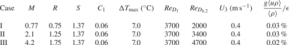
Three separate experiments were performed to study the evolution of multiple scalars and velocity in coaxial jets. Experimental conditions relating to each are summarized in table 3. Momentum flux ratios ( $M=M_2/M_1$) were varied from 0.77 to 4.2, such that coaxial jets in which $M<1$ and those in which $M>1$ could be studied. In each experiment, the momentum flux (and Reynolds number) of the centre jet was held constant. The centre jet was supplied with a mixture composed of 6 % helium and 94 % air by mass ( $C_1=0.06$), and the coflow was heated such that there was a $7.0\,^{\circ }$C difference in temperature between the coflow and centre jet ( ${\rm \Delta} T_{max}=T_3 - T_1 = 7.0\,^{\circ }$C, where $T_1$ and $T_3$ are the temperatures at the exits of the centre jet and coflow, respectively). The combined buoyancy effects of these scalars were verified to be negligible, as the ratio of production of turbulent kinetic energy by buoyancy to the dissipation rate of turbulent energy ( ${g\langle u\rho \rangle }/{\langle \rho \rangle }/ \epsilon$) was estimated to be at most 0.03 %. Accordingly, both temperature ( $T$) and helium concentration ( $C$) could be considered passive scalars.
Properties of the flow in the centre jet, annular jet and coflow for the three cases investigated, including the momentum flux ( $M=M_2/M_1$), velocity ( $R= U_2/U_1$) and density ( $S = \rho _2/\rho _1$) ratios of the centre and annular jets, the He mass fraction at exit of the centre jet ( $C_1$), the temperature difference between the centre jet and coflow ( ${\rm \Delta} T_{{max}} = T_3-T_1$), the Reynolds number of the centre and annular jets (respectively $Re_{D_1}$, $Re_{D_{h,2}}$), the velocity of the coflow ( $U_3$) and the maximum ratio of production of turbulent kinetic energy by buoyancy ( $g\langle u\rho \rangle /\langle \rho \rangle$) to the dissipation of turbulent kinetic energy ( $\epsilon$).
In the present work, the scalars were normalized to be equal to 1 at their respective jet exits:  $\phi _1=C/C_1$ and $\phi _3=(T-T_1)/{\rm \Delta} T_{max}$, thus effectively representing the mixture fraction of these flows. (See Bilger & Dibble (Reference Bilger and Dibble1982) for further information on mixture fractions.) For flows in which multiple scalars are mixed, such as the present one, the flow can be thought of as $n$ scalars mixing in an additional fluid, or as $n+1$ scalars, where the additional fluid also transports a scalar (Cai et al. Reference Cai, Dinger, Li, Carter, Ryan and Tong2011; Rowinski & Pope Reference Rowinski and Pope2013; Li et al. Reference Li, Yuan, Carter and Tong2017). The latter convention is used in this work, and the flow is accordingly viewed as containing a total of three scalars, where $\phi _2$ represents the fluid (or ‘scalar’) of the (cold, helium-free) annular jet. This scalar may be inferred from measurements of the other two assuming that (i) differential diffusion is negligible, (ii) all excess temperature originates from the coflow and (iii) the ambient (unheated) air surrounding the coflow does not penetrate the measurement domain. Since the scalars are defined as mixture fractions, they must sum to one, such that (Rowinski & Pope Reference Rowinski and Pope2013)
 \begin{equation} \phi_2=1-\phi_1-\phi_3. \end{equation}
Thus, the annular fluid denoted by  $\phi _2$ may be differentiated from the centre jet and coflow fluids by the absence of helium concentration and excess temperature.
Simultaneous measurements of  $U$,
$U$,  $\phi _1$, $\phi _2$ and $\phi _3$ were recorded along the axis of the coaxial jets at locations in the range $1.6\leq x/D_1 \leq 25.1$. Given the complexity and novelty involved in simultaneously measuring multiple scalars and velocity, especially in turbulent flows, measurements presented herein are restricted to the axis of the jets to minimize any effects of the larger turbulence intensities off the axis of the jets. The results of these measurements are presented in the following section.
5. Results
5.1. Mean quantities
The downstream evolution of the mean quantities ( $\langle U \rangle$, $\langle \phi _1 \rangle$, $\langle \phi _2 \rangle$, $\langle \phi _3 \rangle$) is presented in figure 3. Similarly to previous studies of the velocity field of coaxial jets, we find that the centreline of coaxial jets can be characterized by three distinct regions (see figure 1): (i) the potential core of the centre jet, (ii) the inner mixing region where the centre and annular jets mix with each other but not with the coflowing fluid and (iii) the fully merged region, where the flow resembles that of a single jet with the same initial momentum. The behaviour of the flow in the aforementioned regions is first described by using $\langle U \rangle$, $\langle \phi _1 \rangle$, $\langle \phi _2 \rangle$ and $\langle \phi _3 \rangle$, before examining the effect that $M$ has on the evolution of these quantities.
Downstream evolution of (a)  $\langle U \rangle$, (b) $\langle \phi _1 \rangle$, (c) $\langle \phi _2 \rangle$ and (d) $\langle \phi _3 \rangle$ along the centreline. Note that measurements of $\langle U \rangle$ are non-dimensionalized using $U_1$, the average velocity at the exit of the centre jet and that the dashed lines delineate the three regions of the jet (the potential core of the centre jet, inner mixing region and fully merged region).

5.1.1. Potential core of the centre jet
As may be observed in figure 3,  $\langle \phi _1 \rangle \approx 1$, $\langle \phi _2 \rangle \approx 0$ and $\langle \phi _3 \rangle \approx 0$ along the axis and immediately beyond the exit of the centre jet. The potential core of this jet is characterized by the region in which $\phi =1$, and generally extends a few diameters beyond its exit. Villermaux & Rehab (Reference Villermaux and Rehab2000) suggest that it may be defined to end where $\langle \phi _1 \rangle =0.9$, which in the present work corresponds to a downstream position of $1.6 < x/D_1 < 3.2$. Consistent with previous studies of coaxial jets (e.g. Rehab et al. Reference Rehab, Villermaux and Hopfinger1997; Favre-Marinet et al. Reference Favre-Marinet, Camano and Sarboch1999; Favre-Marinet & Schettini Reference Favre-Marinet and Schettini2001; Schumaker & Driscoll Reference Schumaker and Driscoll2012), one may infer from figure 3(b) that the potential core of the centre jet decreases as $M$ increases.
5.1.2. Inner mixing region
Just beyond the potential core of the centre jet,  $\langle \phi _1 \rangle$ decreases, while $\langle \phi _2 \rangle$ and $\langle \phi _3 \rangle$ both increase. Although the scalars evolve similarly for all three cases, this is not true of $\langle U \rangle$. In case I, $\langle U \rangle$ immediately decreases; in case II, $\langle U \rangle$ remains constant until $x/D_1\approx 6.4$ before decreasing; and in case III, $\langle U \rangle$ increases until $x/D_1=6.4$ and then starts to decrease. The behaviour described above is consistent with the inner mixing region, which herein is defined to be the region of flow dominated by mixing between the centre and annular jets, and therefore consists primarily (but not necessarily entirely) of $\phi _1$ and $\phi _2$. For example, where the centre and annular jets mix with each other, but not the coflow, $\phi _1+\phi _2 \approx 1$, and $\langle \phi _2 \rangle$ is expected to increase as $\langle \phi _1 \rangle$ decreases. As can be seen in figures 3(b) and 3(c), this occurs until approximately $6.4 \leq x/D_1 \leq 8.0$. Moreover, for coaxial jets in which $R>1$, it is expected that mixing with the faster annular jet will cause the mean centreline velocity to increase where the coflow has not yet reached the centreline. This can be observed for case III ( $R=1.75$, $M=4.2$), and to a limited extent case II ( $R=1.25$, $M=2.1$), before $x/D_1=6.4$.
5.1.3. Fully merged region
As may be observed in figure 3,  $\langle U \rangle$, $\langle \phi _1 \rangle$ and $\langle \phi _2 \rangle$ all decrease beyond $x/D_1 \approx 6.4$, and $\langle \phi _3 \rangle$ increases, similarly to what one would observe in a single jet of $\phi _1$ and $\phi _2$ emanating into a flow of $\phi _3$. In the present work, $x/D_1=6.4$ is therefore assumed to mark the end the inner mixing region and the beginning of the fully merged region.
5.1.4. Effects of  $M$ on the evolution of $\langle U \rangle$, $\langle \phi _1 \rangle$, $\langle \phi _2 \rangle$ and $\langle \phi _3 \rangle$


Increasing the momentum flux ratio causes (i)  $\langle \phi _1 \rangle$ to decay more quickly, (ii) $\langle \phi _2 \rangle$ to initially increase more rapidly and to higher values and (iii) $\langle \phi _3 \rangle$ to increase slightly more slowly. Additionally $\langle U \rangle /U_1$ decays more rapidly as $M$ decreases. The evolutions of $\langle \phi _1 \rangle$ and $\langle U \rangle$ with respect to $M$ are explained by the fact that the momentum and streamwise scalar flow rates are conserved throughout the flow. (These are, respectively $\approx \int _{-\infty }^{\infty } 2{\rm \pi} r \rho \langle U \rangle ^2 \,{\rm d} r$ and $\approx \int _{-\infty }^{\infty } 2{\rm \pi} r \rho \langle U \rangle \langle \phi \rangle \,{\rm d} r$, since the turbulent components can be assumed to be negligible, like in single jets.) Given that the total momentum flow rate increases with $M$, and assuming (i) constant fluid properties (a reasonable assumption as the scalars are considered to be passive) and (ii) that coaxial jets are expected to spread at same rate independent of $M$ (demonstrated in Champagne & Wygnanski Reference Champagne and Wygnanski1971; Ko & Au Reference Ko and Au1982), then $\langle U \rangle$ should increase with $M$ at a given downstream position. Likewise, as the streamwise scalar flow rate of $\phi _1$ is independent of $M$ (since the properties of the centre jet are held constant for all three cases), then $\langle \phi _1 \rangle$ should decrease to compensate for the increase in $\langle U \rangle$. Since $M$ is increased by increasing the initial momentum flux of the annular jet ( $M_2$, and thus $U_2$), the streamwise scalar flow rate of $\phi _2$ increases with $M$. It is therefore not surprising to observe more significant amounts of $\langle \phi _2 \rangle$ on the centreline for larger values of $M$. Interestingly, differences in the values of $\langle \phi _1 \rangle$ and $\langle \phi _2 \rangle$ are greater when comparing case II ( $M=2.1$) with case I ( $M=0.77$) than when comparing it with case III ( $M=4.2$), even though differences in the magnitudes of $M$ are smaller and those in the magnitudes of $R$ are equivalent.
Trends in  $\langle \phi _1 \rangle$ and $\langle \phi _2 \rangle$ with respect to $M$ are consistent with those observed by Li et al. (Reference Li, Yuan, Carter and Tong2017) for coaxial jets in which $M<1$ and $M_2$ is varied, as well those observed by Villermaux & Rehab (Reference Villermaux and Rehab2000) for jets in which $M>1$. Both Li et al. (Reference Li, Yuan, Carter and Tong2017) and Villermaux & Rehab (Reference Villermaux and Rehab2000) showed that $\langle \phi _1 \rangle$ decreases more quickly as $M$ increases, and Li et al. (Reference Li, Yuan, Carter and Tong2017) additionally found that $\langle \phi _2 \rangle$ peaks at higher values with increasing $M$. Furthermore, Warda et al. (Reference Warda, Kassab, Elshorbagy and Elsaadawy2001) also demonstrated that $\langle U \rangle /U_1$ decayed more quickly as $M$ is reduced. However, in contrast to the present results, Li et al. (Reference Li, Yuan, Carter and Tong2017) showed that $M$ had no effect on the evolution of $\langle \phi _3\rangle$ for jets with small diameter ratios ( $D_2/D_1=1.51$), and $\langle \phi _3 \rangle$ increased more quickly with increasing $M$ for jets with larger diameter ratios ( $D_2/D_1=1.97$).
5.2. Second-order quantities
This subsection describes the evolution of various second-order quantities, including root-mean-square (r.m.s.) quantities ( $u_{rms}$, $\phi _{1,rms}$, $\phi _{2,rms}$, $\phi _{3,rms}$), fluctuation intensities ( $u_{rms}/\langle U \rangle$, $\phi _{1,rms}/\langle \phi _1 \rangle$, $\phi _{2,rms}/\langle \phi _2 \rangle$, $\phi _{3,rms}/\langle \phi _3 \rangle$) and correlation coefficients ( $\rho _{u\phi _1}$, $\rho _{u\phi _2}$, $\rho _{u\phi _3}$, $\rho _{\phi _1\phi _2}$, $\rho _{\phi _1\phi _3}$, $\rho _{\phi _2\phi _3}$).
5.2.1. The r.m.s. quantities
The r.m.s. profiles of  $U$,
$U$,  $\phi _1$, $\phi _2$ and $\phi _3$ are presented in figure 4. As depicted in figure 4(a), $u_{rms}$ exhibits a local maximum in the range $3.2< x/D_1<4.8$, just beyond the end of the inner potential core; a local minimum at $4.8< x/D_1<6.4$, towards the end of the inner mixing region; and a second, much larger, local maximum in the fully merged region between $x/D_1=9.6$ and $x/D_1=16.1$. The first local maximum approximately coincides with the maximum values of $\phi _{1,rms}$ and $\phi _{2,rms}$. Previous studies also show scalar fluctuations peaking in the inner mixing region (i.e. following the end of potential core of the centre jet; Balarac et al. Reference Balarac, Si-Ameur, Lesieur and Métais2007; Cai et al. Reference Cai, Dinger, Li, Carter, Ryan and Tong2011; Li et al. Reference Li, Yuan, Carter and Tong2017), most likely due to large-scale vortices associated with the Kelvin–Helmholtz layer that forms at the mixing layer between the between the centre and annular jets. According to Champagne & Wygnanski (Reference Champagne and Wygnanski1971), the (normalized) r.m.s. velocity can be observed to reach a minimum value at the axial position approximately corresponding with the disappearance of the annular jet's potential core, which would suggest that this core ends somewhere in the range $4.8< x/D_1<6.4$ in the present experiments. Finally, the second local maximum of $u_{rms}/U_1$ appears to coincide with that of $\phi _{3,rms}$, with both occurring where the two inner jets are assumed to begin mixing with the coflow. Significant variability can be observed in the near-field evolution of $u_{rms}$ in previous studies, making comparison with the current work difficult (e.g. Champagne & Wygnanski Reference Champagne and Wygnanski1971; Buresti et al. Reference Buresti, Talamelli and Petagna1994, Reference Buresti, Petagna and Talamelli1998; Warda et al. Reference Warda, Kassab, Elshorbagy and Elsaadawy1999, Reference Warda, Kassab, Elshorbagy and Elsaadawy2001). For example, data obtained by Champagne & Wygnanski (Reference Champagne and Wygnanski1971) demonstrated that $u_{rms}$ exhibits two local maxima in jets if the annular jet's core ends after that of the centre jet, but only a single maximum if the opposite occurs. Herein, it can be seen that increasing $M$ increases the magnitude of all fluctuations and delays the location at which maximum values of $u_{rms}/U_1$ and $\phi _{3, rms}$ occur. Similarly, Li et al. (Reference Li, Yuan, Carter and Tong2017) also found that increasing $M$ increased fluctuations of $\phi _{1,rms}$ and $\phi _{2,rms}$, which they credited to increased production rates in coaxial jets in which $M$ is larger. However, we should note that their assessment was only based on an examination of the scalar cross-stream profiles, despite the fact that production rates also depend on values of the scalar fluxes, which were not measured therein.
Downstream evolution of (a)  $u_{rms}/U_1$, (b) $\phi _{1,rms}$, (c) $\phi _{2,rms}$ and (d) $\phi _{3,rms}$ along the centreline. Note that the dashed lines delineate the three regions of the jet (the potential core of the centre jet, inner mixing region and fully merged region).

5.2.2. Fluctuation intensities
The profiles of  $u_{rms}$, $\phi _{1,rms}$, $\phi _{2,rms}$ and $\phi _{3,rms}$ are non-dimensionalized by their mean values in figure 5, yielding profiles of the fluctuation intensities. Although the evolutions of $u_{rms}/\langle U \rangle$, $\phi _{2,rms}/\langle \phi _2 \rangle$, $\phi _{3,rms}/\langle \phi _3 \rangle$ are similar for different values of $M$, those of $\phi _{1,rms}/\langle \phi _1 \rangle$ are distinct. In cases I and II, only a single peak in $\phi _{1,rms}/\langle \phi _1 \rangle$ is observed, but in the former case it is much lower, and occurs farther downstream. Grandmaison et al. (Reference Grandmaison, Becker and Zettler1996), Cai et al. (Reference Cai, Dinger, Li, Carter, Ryan and Tong2011) and Li et al. (Reference Li, Yuan, Carter and Tong2017) each observed evolutions of $\phi _{1,rms}/\langle \phi _1 \rangle$ like those depicted for cases I and II, and Li et al. (Reference Li, Yuan, Carter and Tong2017) showed that the peak of $\phi _{1,rms}/\langle \phi _1 \rangle$ in the near field was (i) stronger when the annular jet was larger, and (ii) disappeared when $M$ was much less than 1. Inspection of the results herein, as well as those of Grandmaison et al. (Reference Grandmaison, Becker and Zettler1996), Cai et al. (Reference Cai, Dinger, Li, Carter, Ryan and Tong2011) and Li et al. (Reference Li, Yuan, Carter and Tong2017) suggests that the peak of $\phi _{1,rms}/\langle \phi _1 \rangle$ occurs just beyond the potential core of the centre jet, in the inner mixing region. In (single) jets, it should be noted that a similar, but much smaller peak in $\phi _{rms}/\langle \phi \rangle$ occurs just beyond the potential core of (single) smooth contraction nozzle jets (with a top-hat velocity profile at the jet exit) due to highly coherent vortex structures present in the near-field. Strong large-scale engulfment of the ambient fluid by these structures results in large scalar fluctuations and quick growth of $\phi _{rms}$ (compared with fully developed pipe jets, where there are few or no large-scale coherent structures; Mi, Nobes & Nathan Reference Mi, Nobes and Nathan2001). Similar behaviour likely occurs in coaxial jets, and appears to increase with increasing $M$. In case III, two peaks are observed for $\phi _{1,rms}/\langle \phi _1 \rangle$, the first of which occurs between $x/D_1=3.2$ and $4.8$ – where $\phi _{1,rms}$ reaches a maximum value – and the second of which occurs between $x/D_1=9.6$ and $12.9$ – where $\phi _{3, rms}$ peaks. In this case, there appear to be two regions of intense fluctuations for $\phi _1$: first, where the centre and annular jet begin mixing, and second, where the two inner jets begin mixing with the coflow. The difference between these two regions of fluctuations may occur because increasing $M$ reduces the potential core of the centre jet, and thus the location at which the inner jets first mix. In cases I and II, the inner potential core may be sufficiently long that the two regions are indistinguishable.
Downstream evolution of (a)  $u_{rms}/\langle U \rangle$, (b) $\phi _{1,rms}/\langle \phi _1 \rangle$, (c) $\phi _{2,rms}/\langle \phi _2 \rangle$ and (d) $\phi _{3,rms}/\langle \phi _3 \rangle$ along the centreline. Note that the dashed lines delineate the three regions of the jet (the potential core of the centre jet, inner mixing region and fully merged region).

Far downstream, the centre and annular jets are expected to ultimately behave like a single jet of the same total momentum issuing in quiescent air. (Given the low initial velocity of the coflow, the dynamics of the two inner jets should not be strongly affected.) In the current work, measurements are limited to  $x/D_1 \leq 25.7$, and the asymptotic values are not yet fully achieved. Nevertheless, it can be observed that $u_{rms}/\langle U \rangle$, $\phi _{1,rms}/\langle \phi _1 \rangle$ and $\phi _{3,rms}/\langle \phi _3 \rangle$ all approach their asymptotic values more slowly as $M$ is increased, which suggests that the coaxial jets mix with the coflow more slowly as $M$ increases. The maximum measured values of $u_{rms}/\langle U \rangle$ are 0.21–0.22, and, based on figure 5(a), likely to continue increasing farther downstream. At the same location, $\phi _{1,rms}/\langle \phi _1 \rangle$ is approximately 0.17–0.19 for the three cases, and $\phi _{2,rms}/\langle \phi _2 \rangle$ falls between 0.24 and 0.27. Although these values may be slightly lower (for $u_{rms}/\langle U \rangle$ and $\phi _{1,rms}/\langle \phi _1 \rangle$) or higher (for $\phi _{2,rms}/\langle \phi _2 \rangle$) than those typically observed in the self-similar region of single jets, it must be emphasized that the coaxial jets do not appear to have fully reached self-similarity. Moreover, Cai et al. (Reference Cai, Dinger, Li, Carter, Ryan and Tong2011) and Grandmaison, Pollard & Ng (Reference Grandmaison, Pollard and Ng1991), who also studied the mixing of multiple scalars in coaxial jets, measured asymptotic values of $\phi _{1,rms}/\langle \phi _1 \rangle$ consistent with those of the current work (0.21 and 0.16, respectively). It is possible that even if the behaviour of coaxial jets ultimately resembles that of single jets, differences in their evolution in the near field may nevertheless perpetuate far downstream, similarly to what can be observed when comparing fully developed pipe jets with smooth contraction nozzle jets (see Mi et al. Reference Mi, Nobes and Nathan2001; Xu & Antonia Reference Xu and Antonia2002), and in accordance with analytical arguments put forth by George & Arndt (Reference George and Arndt1989) and George (Reference George2012) about the persistence of initial conditions in a jet.
5.2.3. Correlation coefficients
Velocity-scalar correlation coefficients ( $\rho _{u\phi _1}$, $\rho _{u\phi _2}$, $\rho _{u\phi _3}$) and scalar–scalar correlation coefficients ( $\rho _{\phi _1\phi _2}$, $\rho _{\phi _1\phi _3}$, $\rho _{\phi _2\phi _3}$) are presented in figure 6. One may observe that the velocity-scalar correlation coefficients $\rho _{u\phi _1}$ and $\rho _{u\phi _2}$ are initially approximately $0$, indicating that these quantities are uncorrelated. However, in case III, where velocity differences between the two jets are larger, a local minimum and maximum beyond the centre jet's potential core show $U$ and $\phi _1$ becoming slightly anti-correlated and $U$ and $\phi _2$ becoming slightly positively correlated. In this same region ( $1.6 \leq x/D_1 \leq 4.8$), $\rho _{\phi _1\phi _2}=-1$, such that measurement of $\phi _1$ implies absence of $\phi _2$, and vice versa. This is due to the flow primarily consisting of $\phi _1$ and $\phi _2$ (such that $\phi _1+\phi _2 \approx 1$; see figures 3 and 4). In a binary mixture
 \begin{equation} \langle \phi_{\alpha}'\phi_{\beta}' \rangle ={-}\langle \phi_{\alpha}'^2 \rangle ={-} \langle \phi_{\beta}'^2\rangle, \end{equation}
and the correlation coefficient is therefore  $-$1, by definition. Towards the end of the inner mixing region, as incursions of $\phi _3$ more frequently reach the centreline, $\rho _{\phi _1\phi _2}$ begins increasing, and any trends in $\rho _{u\phi _1}$ and $\rho _{u\phi _2}$ reverse,
Downstream evolution of correlation coefficients along the centreline: (a)  $\rho _{u\phi _1}$, (b) $\rho _{u\phi _2}$, (c) $\rho _{u\phi _3}$, (d) $\rho _{\phi _1\phi _2}$, (e) $\rho _{\phi _1\phi _3}$, ( f) $\rho _{\phi _2\phi _3}$. Given that $\phi _3$ is not expected to be present (at least in significant quantities) before the fully merged region, data for $\rho _{u\phi _3}$, $\rho _{\phi _1\phi _3}$, $\rho _{\phi _2\phi _3}$ are only plotted for $x/D\geq 6.4$. Note that the dashed lines delineate the three regions of the jet (the potential core of the centre jet, inner mixing region and fully merged region).

Beyond the inner mixing region,  $\rho _{u\phi _1}$, $\rho _{u\phi _2}$ and $\rho _{\phi _1\phi _2}$ all increase and tend towards positive values, while $\rho _{u\phi _3}$, $\rho _{\phi _1\phi _3}$, $\rho _{\phi _2\phi _3}$ all decrease and tend towards negative values, similarly to what would occur in a single jet of $\phi _1$ and $\phi _2$ mixing in a fluid of $\phi _3$. Farther downstream, $\rho _{\phi _1\phi _2}$ appears to asymptote to a value of 0.6, whereas other predictions would suggest that $\rho _{\phi _1\phi _2}$ should tend to 1 (e.g. Warhaft Reference Warhaft1984). Given that profiles of the fluctuations intensities show that self-similarity of the jets is not yet reached, it is possible that measurements were not obtained far enough downstream to observe the asymptotic values of $\rho _{\phi _1\phi _2}$. For example, Grandmaison et al. (Reference Grandmaison, Pollard and Ng1991) found that when $M$ was large, $\rho _{\phi _1\phi _2}$ plateaued, and even decreased, before eventually increasing to 1 farther downstream. Moreover, in most previous studies of multi-scalar mixing, upon which our understanding of these processes have been developed, the density of the flow is nearly constant and the scalars have similar or identical diffusivities (e.g. the works of Warhaft Reference Warhaft1984; Grandmaison et al. Reference Grandmaison, Pollard and Ng1991; Tong & Warhaft Reference Tong and Warhaft1995; Costa-Patry & Mydlarski Reference Costa-Patry and Mydlarski2008; Cai et al. Reference Cai, Dinger, Li, Carter, Ryan and Tong2011; Li et al. Reference Li, Yuan, Carter and Tong2017). This is not the case in the current work, and it is not clear, how, or if, these factors have an effect on the evolution of $\rho _{\phi _1\phi _2}$ and its potential asymptotic values.
It is also worth considering the effects of  $M$ on these correlation coefficients, specifically that of $\rho _{\phi _1\phi _2}$. As shown in figure 6(d), when $M$ increases, $\rho _{\phi _1\phi _2}$ increases more rapidly, achieving its asymptotic value faster. These results are somewhat consistent with those of Grandmaison et al. (Reference Grandmaison, Pollard and Ng1991) who found that initially $\rho _{\phi _1\phi _2}$ increased faster as $M$ increased. (In their work, this trend reversed far downstream; $\rho _{\phi _1\phi _2}$ ultimately approached 1 more slowly as $M$ increased.) However, Li et al. (Reference Li, Yuan, Carter and Tong2017) observed the opposite – the scalar correlation coefficients in their experiments evolved more quickly to their asymptotic values as $M$ decreased. The momentum flux ratios investigated in their experiments were approximately 0.94 and 0.47, and they attributed a faster evolution of $\rho _{\phi _1\phi _2}$ at lower velocity ratios to increased shear between the centre and annular jets. However, this would not explain why case II ( $R=1.25$) of the present experiments evolves faster than case I ( $R=0.75$), nor does it explain why the evolution of $\rho _{\phi _1\phi _2}$ in case II is more similar to case III than case I.
5.3. Probability density functions
Non-dimensionalized PDFs of  $U$,
$U$,  $\phi _1$, $\phi _2$ and $\phi _3$ are presented in figures 7–10. These contain information on all statistical moments of each quantity of interest, and can therefore be used to gain additional insight into the behaviour of these quantities. Given that the most unique behaviour of coaxial jets occurs in the near field, measurements in this section focus on the region close to the jet exit ( $x/D_1=1.6$, $3.2$, $4.8$, $6.4$, $9.6$), although the PDFs measured at $x/D_1=25.7$ are also presented to quantify the behaviour of $U$,
$U$,  $\phi _1$, $\phi _2$ and $\phi _3$ far downstream.
Non-dimensionalized PDFs of  $U$ measured along the centreline for case I: $M=0.77$ (——), case II: $M=2.1$ (- - - -), case III: $M=4.2$ (— ${\cdot }$—). Best-fit Gaussian distributions ( $\cdots \cdots$) are also provided for the purpose of comparison. Semi-log plots are presented to highlight the tails of the PDFs.

Non-dimensionalized PDFs of  $\phi _1$ measured along the centreline for case I: $M=0.77$ (——), case II: $M=2.1$ (- - - -), case III: $M=4.2$ (— ${\cdot }$—). Best-fit Gaussian distributions ( $\cdots \cdots$) are also provided for the purpose of comparison.
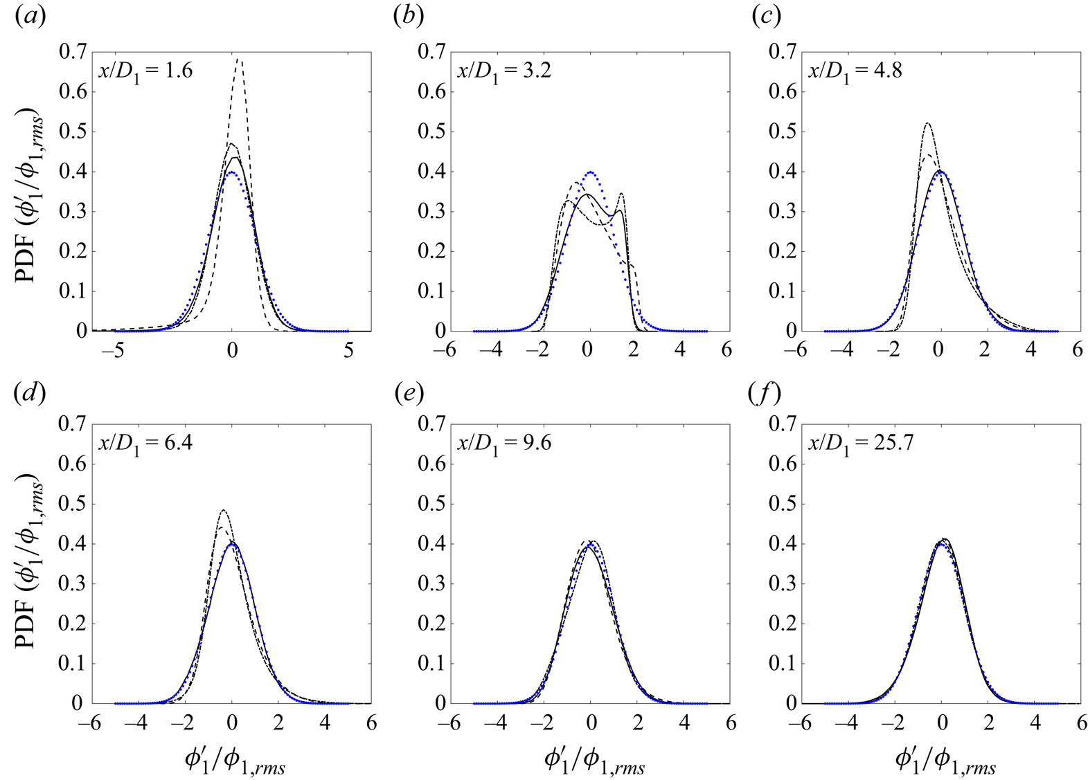
Non-dimensionalized PDFs of  $\phi _2$ measured along the centreline for case I: $M=0.77$ (——), case II: $M=2.1$ (- - - -), case III: $M=4.2$ (— ${\cdot }$—). Best-fit Gaussian distributions ( $\cdots \cdots$) are also provided for the purpose of comparison.

Non-dimensionalized PDFs of  $\phi _3$ measured along the centreline for case I: $M=0.77$ (——), case II: $M=2.1$ (- - - -), case III: $M=4.2$ (— ${\cdot }$—). Best-fit Gaussian distributions ( $\cdots \cdots$) are also provided for the purpose of comparison.

The (non-dimensional) velocity PDFs are quasi-Gaussian, and are not significantly affected by the momentum flux ratio over the ranges studied herein, with the most notable differences being observed in the tails of the PDFs. In the potential core of the centre jet (at  $x/D_1=1.6$), the PDFs are negatively skewed, as a consequence of the fully developed velocity profile at the jet exit and the velocity defect from the wall. (The flow first mixes with fluid from the edges of the centre jet, where the velocity is lower, and this induces negative velocity fluctuations, and therefore negative skewness.) In the inner mixing region ( $3.2 \leq x/D \leq 4.8$), the PDFs are slightly negatively skewed, with the exception of case III at $x/D=3.2$, which is slightly positively skewed. The latter results from mixing with the faster annular jet, which induces increased positive fluctuations, and consequently positive skewness. At the beginning of the fully merged region ( $6.4 \leq x/D \leq 9.6$), the PDFs are less Gaussian, and skewed more negatively, such that large negative velocity fluctuations are more common, implying that the slower moving fluid from the coflow has reached the centreline. Differences in the tails can be observed for the three cases in this region, but by $x/D=25.7$, the velocity PDFs all collapse onto each other. At this location, the PDFs approach a Gaussian distribution, but are not perfectly Gaussian, as is typical for free-shear flows (Pope Reference Pope2000). The evolution of the velocity PDFs presented herein is generally consistent with the centreline skewness and kurtosis data obtained by Buresti et al. (Reference Buresti, Petagna and Talamelli1998) and Sadr & Klewicki (Reference Sadr and Klewicki2003). For a variety of different jets (with different velocity ratios, velocity profiles and geometries), negative skewness can initially observed be close to the jet exit, due to the presence of the wake produced by the jet walls, and again farther downstream, as maximum flow velocities move towards the jet axis. In between, the value of the skewness depends on the velocity ratio of the two jets.
As can be seen in figures 8 and 9, the PDFs of  $\phi _1$ and $\phi _2$ are narrow, with large tails close to the jet exit ( $x/D_1=1.6$). The kurtosis at these locations is therefore large ( $10.3 \leq K_{\phi _1} \leq 22.2$, $8.0 \leq K_{\phi _2} \leq 18.0$), indicating that extreme events occur more frequently. Furthermore, the PDFs of $\phi _1$ are negatively skewed ( $-3.0 \leq S_{\phi _1} \leq -1.1$) at this location, whereas those of $\phi _2$ are positively skewed ( $0.6 \leq S_{\phi _2} \leq 2.7$), which implies that small pockets of $\phi _2$ mix in fluid primarily composed of $\phi _1$. At $x/D_1=3.2$, the PDFs of both $\phi _1$ and $\phi _2$ become bimodal, like those observed by Villermaux & Rehab (Reference Villermaux and Rehab2000) for a scalar injected into the inner of two coaxial jets. One can therefore infer that fluid at $x/D_1=3.2$ consists principally of regions of high $\phi _1$/low $\phi _2$ or low $\phi _1$/high $\phi _2$, an indication of the binary nature of the scalar field close to the jet exit. By $x/D_1=4.8$, the PDFs of $\phi _1$ and $\phi _2$ become unimodal once again, with the former positively skewed and the latter negatively skewed. The degree to which the PDFs of $\phi _1$ are positively skewed and the PDFs of $\phi _2$ are negatively skewed increases with $M$. Pockets of $\phi _1$ mix in a background preferentially composed of $\phi _2$, and this becomes more pronounced as $M$ increases – which suggests that, at least initially, the coaxial jets mix faster as $M$ increases. This behaviour persists farther downstream, but by $x/D=9.6$ the PDFs of the three cases begin to collapse and are less markedly skewed. Far downstream (at $x/D=25.7$), the PDFs of $\phi _1$ and $\phi _2$ are indistinguishable for different values of $M$ and nearly Gaussian.
Given that relatively little  $\phi _3$ is found on the jet axis upstream of the fully merged region, the PDFs of $\phi _3$ are only presented for the following locations: $x/D_1=6.4$, $x/D_1=9.6$ and $x/D_1=25.7$. As may be observed in figure 10, the PDFs of $\phi _3$ are affected by $M$ at the beginning of the fully merged region, but not farther downstream. Moreover, they are positively skewed, indicating that more frequent large, positive fluctuations of $\phi _3$ occur at the centreline, which is where the flow is lowest in $\phi _3$.
5.4. Scalar–scalar JPDFs
Scalar–scalar JPDFs, including the JPDFs of  $\phi _1$ and $\phi _2$ ( $\,f_{\phi _1\phi _2}$), $\phi _1$ and $\phi _3$ ( $\,f_{\phi _1\phi _3}$), and $\phi _2$ and $\phi _3$ ( $\,f_{\phi _2\phi _3}$) are presented in the current subsection. All JPDFs are normalized appropriately (they integrate to 1), and depicted such that the last three contours respectively integrate to 0.99, 0.95 and 0.90.
5.4.1. JPDFs of $\phi _1$ and $\phi _2$


The JPDFs of  $\phi _1$ and $\phi _2$ ( $f_{\phi _1\phi _2}$) were measured at $x/D_1=1.6$, $3.2$, $4.8$, $6.4$, $9.6$ and $25.7$ for each of the three cases. Results are presented in figures 11–13. The evolution of $f_{\phi _1\phi _2}$ along the axis of the coaxial jets is first described. Subsequently, the effects of $M$ on $f_{\phi _1\phi _2}$ are discussed.
5.4.2. Downstream evolution of $f_{\phi _1\phi _2}$

Given that  $\phi _1+\phi _2+\phi _3 = 1$, $\phi _1+\phi _2$ must sum to less than $1$, and the JPDFs should thus be confined to the triangle in the lower-left corner of $\phi _1$– $\phi _2$ space, which is bounded by the points ( $\phi _1=0$, $\phi _2=0$), ( $\phi _1=1$, $\phi _2=0$) and ( $\phi _1=0$, $\phi _2=1$). However, certain small deviations – particularly in the last 3 contours of the JPDFs – can be observed. These are primarily attributed to measurement noise (as was also the case in previous studies; e.g. Cai et al. Reference Cai, Dinger, Li, Carter, Ryan and Tong2011), which is inevitable, especially given the complexity of such 3-component measurements. (See Appendix A for further discussion of the measurement noise.)
JPDFs of  $\phi _1$ and $\phi _2$ for case I ( $M=0.77$). The 3 last contours contain 99 %, 95 % and 90 % of the JPDF. Red lines denote the values of $\langle \phi _1 \rangle$ and $\langle \phi _2 \rangle$.
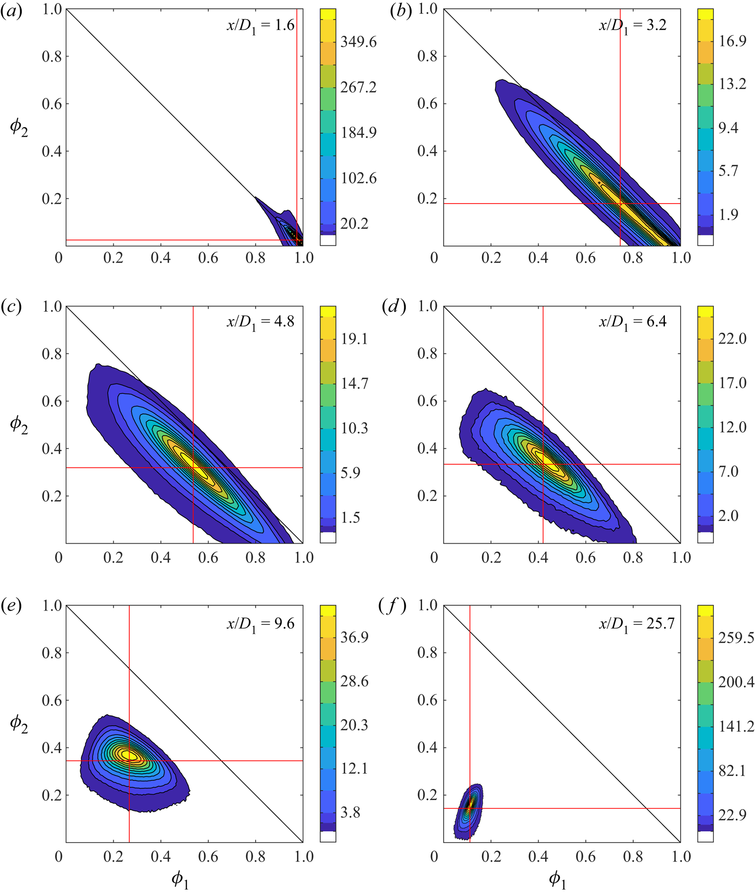
JPDFs of  $\phi _1$ and $\phi _2$ for case II ( $M=2.1$). The 3 last contours contain 99 %, 95 % and 90 % of the JPDF. Red lines denote the values of $\langle \phi _1 \rangle$ and $\langle \phi _2 \rangle$.

JPDFs of  $\phi _1$ and $\phi _2$ for case III ( $M=4.2$). The 3 last contours contain 99 %, 95 % and 90 % of the JPDF. Red lines denote the values of $\langle \phi _1 \rangle$ and $\langle \phi _2 \rangle$.

As depicted in figures 11–13,  $f_{\phi _1\phi _2}$ exhibits similar general trends for the three cases investigated herein ( $M=0.77$, $M=2.1$, $M=4.2$). Close to the jet exit ( $x/D_1=1.6$), the JPDF is mainly concentrated in the lower-right corner of the $\phi _1$– $\phi _2$ scalar space, where $\phi _1 \approx 1$ and $\phi _2 \approx 0$, as consistent with both the underlying physics of the flow and the mean profiles of $\phi _1$ and $\phi _2$. Nevertheless, the first indications of mixing can already be observed at this point, as the JPDFs begin to extend along the line defined of $\phi _1+\phi _2=1$. Mixing between $\phi _1$ and $\phi _2$ becomes enhanced at $x/D_1=3.2$, where the JPDF extends much farther into $\phi _1$– $\phi _2$ scalar space. At this downstream location, $\phi _1$ and $\phi _2$ are still mostly distributed along the $\phi _1+\phi _2=1$ line, demonstrating the anti-correlated nature of $\phi _1$ and $\phi _2$. Moreover, the JPDFs are bimodal, like the PDFs of $\phi _1$ and $\phi _2$ at this location. The JPDF remains anti-correlated at $x/D=4.8$, but moves off the $\phi _1+\phi _2=1$ line, indicating that fluid from the coflow ( $\phi _3$) has begun to reach the centreline. In cases II and III, the JPDF slightly extends towards lower values of $\phi _1$ and $\phi _2$, and continues to do so at $x/D=6.4$. By $x/D=9.6$, $\phi _1$ and $\phi _2$ are no longer anti-correlated and the JPDFs have a rounder, but not Gaussian, shape. Finally, far downstream, the JPDFs have moved to the corner defined by $(\phi _1, \phi _2) = (0,0)$, and the scalars are positively correlated, as may be inferred from the positive slope of the principal axis of the JPDFs.
Close to the jet exit, the evolution of the JPDFs in the current work ( $D_2/D_1=2.1$) is similar to what Li et al. (Reference Li, Yuan, Carter and Tong2017) observed for coaxial jets with similar diameter ratios ( $D_2/D_1=2.0$), but differs from what they observed for coaxial jets with smaller diameter ratios ( $D_2/D_1=1.5$). In the former case, $\phi _1$ and $\phi _2$ were anti-correlated, and the JPDFs first evolved along the line defined by $\phi _1+\phi _2=1$. In contrast, when the diameter ratio was smaller, the JPDFs moved away from this line immediately beyond the end of the centre jet's potential core, indicating an earlier presence of the coflow fluid along the axis. As the diameter ratio decreases, so too does the length of the outer potential core and reattachment point (Champagne & Wygnanski Reference Champagne and Wygnanski1971; Au & Ko Reference Au and Ko1987), which allows $\phi _3$ to reach the centreline much earlier. Farther downstream, the evolution and shapes of the JPDFs herein differ from both cases examined in Li et al. (Reference Li, Yuan, Carter and Tong2017), which underlines the importance that other initial conditions, such as $M$, have on the mixing of $\phi _1$ and $\phi _2$.
5.4.3. Effects of the momentum flux ratio on $f_{\phi _1\phi _2}$

The effects of the momentum flux ratio on the evolution of  $f_{\phi _1\phi _2}$ is examined in more detail for the following select locations: (i) $x/D_1=3.2$, just beyond the end of the potential core, and where fluctuations of $\phi _1$ and $\phi _2$ are largest, (ii) $x/D_1=6.4$, which marks the end of the inner mixing region and the beginning of the fully merged region and (iii) $x/D_1=25.7$, the farthest downstream location at which measurements were obtained. JPDFs at the previously mentioned downstream locations are replotted side by side in figure 14 to more effectively compare the effects of $M$ on the mixing of $\phi _1$ and $\phi _2$. It is worth pointing out that at $x/D_1=3.2$, $6.4$ and $25.7$, $\rho _{\phi _1\phi _2}$ is approximately equal for each of the three momentum fluxes. (At $x/D=3.2$, $-0.98 \leq \rho _{\phi _1\phi _2} \leq -0.97$; at $x/D_1=6.4$, $-0.82 \leq \rho _{\phi _1\phi _2} \leq -0.66$; at $x/D_1=25.7$, $0.56 \leq \rho _{\phi _1\phi _2} \leq 0.57$.) Yet the JPDFs at these locations are not identical. Thus it is clearly demonstrated that the correlation coefficients do not fully describe the state of mixing between scalars.
Effect of the momentum ratio ( $M$) on the JPDFs of $\phi _1$ and $\phi _2$ at $x/D_1=3.2$, $x/D_1=6.4$ and $x/D_1=25.7$. Red lines denote the values of $\langle \phi _1 \rangle$ and $\langle \phi _2 \rangle$. Note that the data of figures 11–13 are replotted here to more effectively compare the effects of $M$.
$M$.

At  $x/D_1=3.2$, the JPDFs of cases II and III extend much farther along the line defined by $\phi _1+\phi _2=1$ than for case I, such that the range of possible values for $\phi _1$ and $\phi _2$ (i.e. 0 to 1) is almost fully spanned for these two cases. Additionally, the location of the peaks of the JPDFs, which indicate the most likely values $\phi _1$ and $\phi _2$ in the flow, shift with increasing $M$. Examination of figure 14(a–c) suggests that at $x/D_1=3.2$, mixing is progressing fastest for case II, where the JPDF is centred around $(\phi _1, \phi _2) \approx (0.45,0.55)$. This is followed by case III, where the flow is very likely to consist of either low $\phi _1$ and high $\phi _2$ or fluid from the centre jet ( $\phi _1=1$, $\phi _2=0$). The slowest mixing occurs for case I, where the JPDF retains its bimodal nature, but is mostly composed of high $\phi _1$ and low $\phi _2$ scalars. Fast mixing of $\phi _1$ and $\phi _2$ in case II can be attributed to the presence of the wake created by the wall separating the two jets, which, as noted in § 2.2, plays an important role in the flow dynamics when the velocity ratio is close to 1. The delayed mixing of $\phi _1$ and $\phi _2$ in case I is explained by the fact that the inner potential core increases as $M$ decreases. By $x/D_1=6.4$, one can observe that as $M$ increases, (i) the peaks of JPDFs move towards lower values of $\phi _1$ and higher values of $\phi _2$, consistent with the mean profiles of these quantities, (ii) these peaks move more slowly off the line defined by $\phi _1+\phi _2=1$ and (iii) the JPDFs progressively extend towards $(\phi _1, \phi _2) = (0,0)$, their final (asymptotic) state, indicating an increased presence of large, but rare, fluctuations of $\phi _3$ that mix $\phi _1$ and $\phi _2$ together. Finally, as depicted in figure 14(g–i), at $x/D_1=25.7$, the JPDFs become thinner and longer as $M$ gets larger, since fluctuations of $\phi _1$ decrease and those of $\phi _2$ increase. The JPDF of case I is centred at $(\phi _1, \phi _2) \approx (0.1,0.2)$, closest to $(\phi _1, \phi _2) = (0,0)$, and has a shape that appears to approach a joint-normal distribution, which is expected when scalars are well mixed (Juneja & Pope Reference Juneja and Pope1996). Thus, far downstream, this case is presumably better mixed than the other two.
Consequently, one may infer that mixing between  $\phi _1$ and $\phi _2$ initially progresses faster for cases II and III, where $M$ is larger, but farther downstream, it appears to progress faster for case I. The former can be explained by the reduced inner core length of such cases, and is further supported by the previously discussed profiles of $\rho _{\phi _1\phi _2}$, which indicated that $\phi _1$ and $\phi _2$ mix faster as $M$ increases in the range of $4.8 < x/D_1 < 22.5$. The latter agrees with the results of Li et al. (Reference Li, Yuan, Carter and Tong2017) for coaxial jets in which $M<1$. Li et al. (Reference Li, Yuan, Carter and Tong2017) found that as $M$ (
$M$ ( $R$ in their constant-density experiments) increased, the JPDF moved farther into the $\phi _1$– $\phi _2$ scalar space, and towards smaller values of $\phi _1$. However, farther downstream their scalars were more fully mixed for the case with a lower value of $M$. From their results, they concluded that turbulent transport (i.e. transport by the conditional mean of the fluctuating velocity) increased with increasing $M$, which initially caused the JPDFs to evolve faster. However, small-scale mixing was slower, and delayed the evolution of JPDFs far downstream.
5.4.4. JPDFs of $\phi _1$ and $\phi _3$


Similarly to the PDFs of  $\phi _3$, the JPDFs of $\phi _1$ and $\phi _3$ were only measured at $x/D_1=6.4$, $9.6$ and $25.7$ for each of the three cases. The results are presented in figure 15, and we reiterate that the JPDFs of $\phi _1$ and $\phi _3$ should be confined to the triangle in the lower-left corner of $\phi _1$– $\phi _3$ space, since $\phi _1+\phi _2+\phi _3=1$. As $x/D_1$ increases, $f_{\phi _1\phi _3}$ moves from the bottom of $\phi _1$– $\phi _3$ scalar space, where $\phi _3$ is small, to the top-left corner of $\phi _1$– $\phi _3$ scalar space, where $\phi _1$ is small and $\phi _3$ is large, consistent with previous results presented herein. Like the measurements of $f_{\phi _1\phi _2}$ in the previous subsection, both the shape and evolution of $f_{\phi _1\phi _3}$ depend on $M$. For example, at $x/D_1=6.4$, as $M$ increases, the peak of the JPDF moves closer to $(\phi _1,\phi _3)=(0,0)$, due to increasing amounts of $\phi _2$ at this location (see figure 3c). Additionally, its shape approaches that of a right triangle when $M>1$, such that one may also observe instances where the flow consists only of $\phi _1$– $\phi _2$ mixtures or only of $\phi _2$– $\phi _3$ mixtures. There are no mixtures consisting of only $\phi _1$ and $\phi _3$ because these two scalars must first mix with $\phi _2$ before being able to mix with each other. The evolution of $f_{\phi _1\phi _3}$ when $M$ is large therefore bears some resemblance to the evolution of the scalar–scalar JPDFs observed in the work of Soltys & Crimaldi (Reference Soltys and Crimaldi2015), where two parallel jets mix in a slow-moving coflow. Soltys & Crimaldi (Reference Soltys and Crimaldi2015) found that the scalar–scalar JPDFs evolved along the axes of scalar space (i.e. lines defined by $\phi _1=0$ and $\phi _3=0$), and coalescence of the scalars only occurred after significant dilution with the ambient fluid. The situation herein is slightly different, given that $\phi _2$ is not present in sufficient quantity to permit $\phi _1$ and $\phi _3$ to effectively mix. However, one can nevertheless observe a tendency for $f_{\phi _1\phi _3}$ to evolve along the axes of scalar space (at least for $M>1$).
JPDFs of  $\phi _1$ and $\phi _3$. The 3 last contours contain 99 %, 95 % and 90 % of the JPDF. Red lines denote the values of $\langle \phi _1 \rangle$ and $\langle \phi _3 \rangle$.
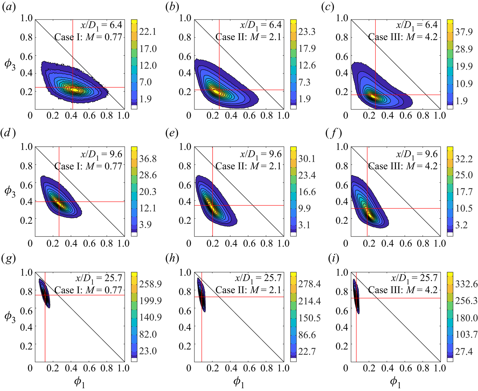
5.4.5. JPDFs of $\phi _2$ and $\phi _3$


The JPDFs of  $\phi _2$ and $\phi _3$ were also measured at $x/D_1=6.4$, $9.6$ and $25.7$ for the three cases investigated herein. As can be seen in figure 16, at $x/D_1=6.4$, which marks the location at which $\langle \phi _2 \rangle$ reaches its maximum value, quasi-triangular JPDF shapes are again observed when $M>1$. In this case, the JPDF is bounded on one side by $\phi _3=0$, indicating the presence of a mixture purely composed of $\phi _1$ and $\phi _2$, and on the other by $\phi _2+\phi _3=1$, indicating the presence of a mixture purely composed of $\phi _2$ and $\phi _3$. At $x/D_1=9.6$, the JPDFs move towards this line for cases in which $M>1$, and by $x/D_1=25.7$, the JPDFs of all cases are nearly aligned with ${\phi _2+\phi _3=1}$. Although the flow appears to mainly consist of anti-correlated $\phi _2$ and $\phi _3$, it is important to note that $\phi _1$ is still present, albeit in small quantities. These results, along with those for $f_{\phi _1\phi _3}$, demonstrate that there appear to exist differences in the near-field evolution of coaxial jets in which $M<1$ and those in which $M>1$. In case I (when $M<1$), all three scalars are generally present and mix together in the fully merged region, as indicated by the fact that the JPDFs evolve through the centre of scalar space. However, in cases II and III (when $M>1$), there exist regions of flow in which $\phi _1$ or $\phi _3$ may be absent.
The JPDFs of  $\phi _2$ and $\phi _3$. The 3 last contours contain 99 %, 95 % and 90 % of the JPDF. Red lines denote the values of $\langle \phi _2 \rangle$ and $\langle \phi _3 \rangle$.
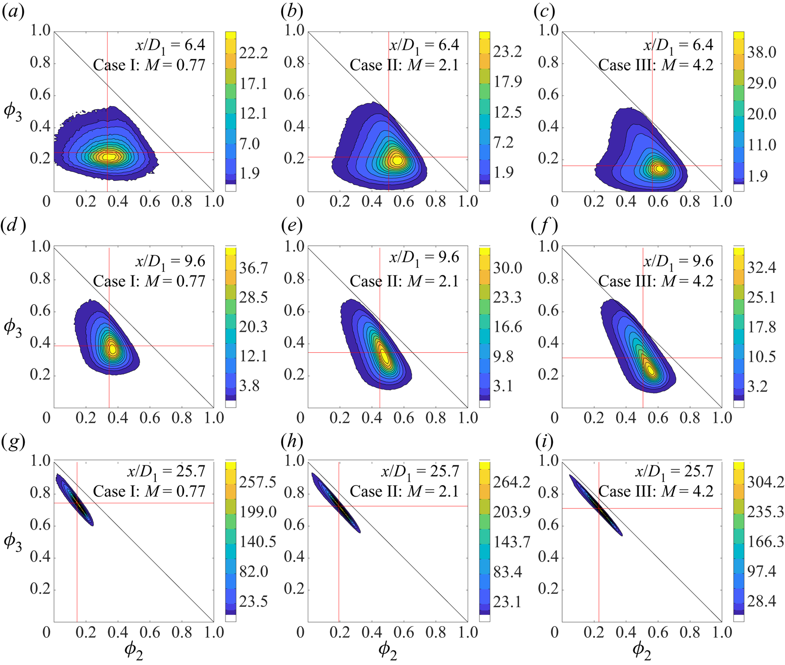
5.5. Velocity-scalar JPDFs
The JPDFs of  $U$ and $\phi _1$ ( $f_{U\phi _1}$), $U$ and $\phi _2$ ( $f_{U\phi _2}$) and $U$ and $\phi _3$ ( $f_{U\phi _3}$) are presented in non-dimensionalized form in figures 17, 18, 19, respectively. Measurement noise and errors are expected to occur in the same regions as those in which they were observed for the scalar–scalar JPDFs. The bimodal nature of the flow at $x/D_1=3.2$ – that is, its tendency to be composed of high $\phi _1$/low $\phi _2$ or low $\phi _1$/high $\phi _2$ – can again be observed in the velocity-scalar JPDFs, and is shown to occur nearly independently of velocity. Furthermore, as previously discussed in § 5.2, the velocity and scalar fields appear to be uncorrelated at this point. Farther downstream $f_{U\phi _1}$ and $f_{U\phi _2}$ both evolve such that they eventually become positively inclined. Although this reflects trends observed in the evolutions of $\rho _{U\phi _1}$ and $\rho _{U\phi _2}$, it is important to note that like in the case of $\rho _{\phi _1\phi _2}$, these correlation coefficients do not fully describe the state of the flow. For example, at $x/D_1=9.6$, the correlation coefficients do not show that when $M>1$, positive correlation of $U$ and $\phi _1$ occurs where velocity fluctuations are negative, but not necessarily where they are positive. Moreover, although both $\rho _{U\phi _1}$ and $\rho _{U\phi _2}$ evolve similarly, and frequently have similar values, the shapes and evolutions of $f_{U\phi _1}$ and $f_{U\phi _2}$ are distinct in the near field.
Non-dimensionalized JPDFs of  $U$ and $\phi _1$. The 3 last contours contain 99 %, 95 % and 90 % of the JPDF.
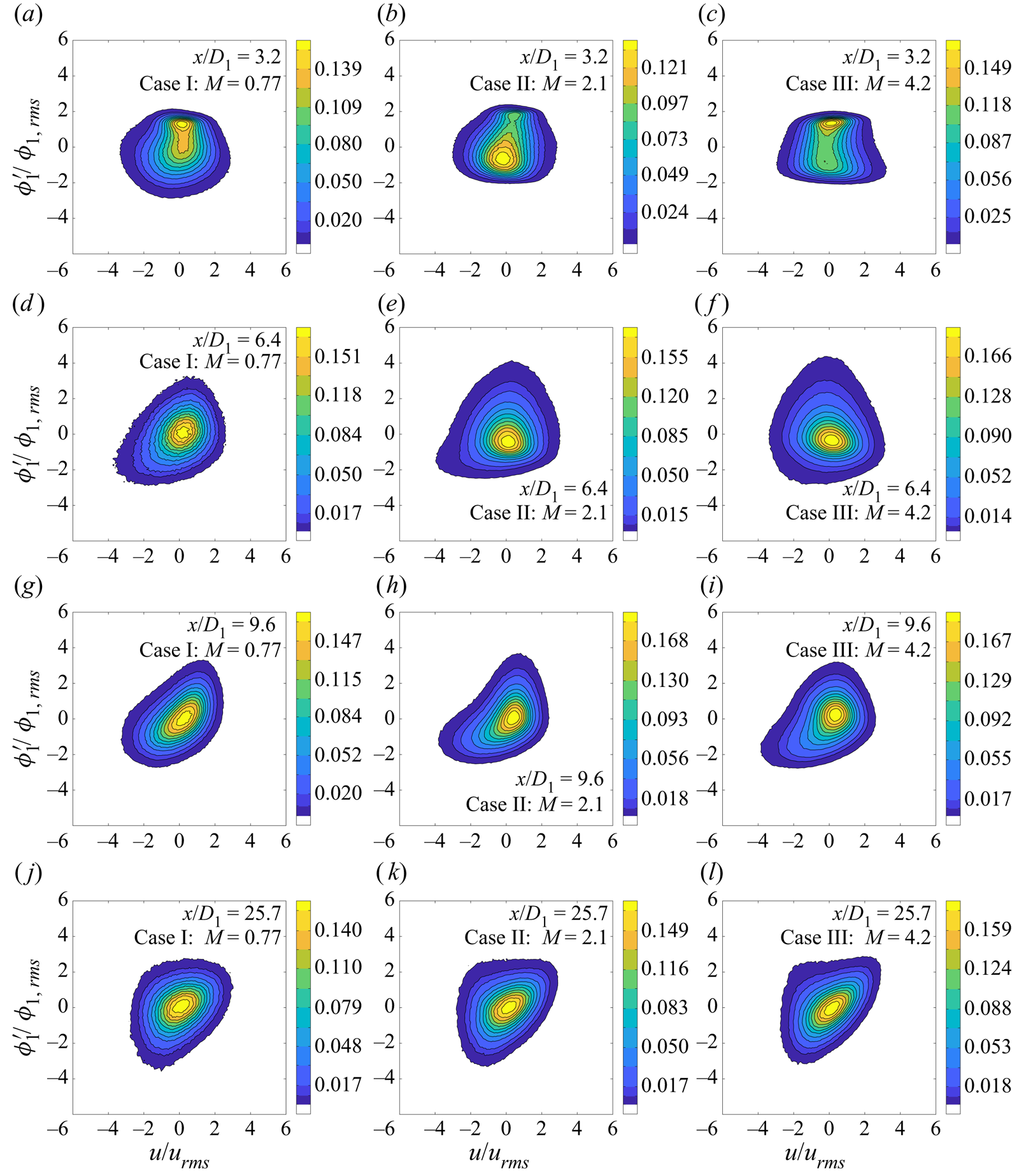
Non-dimensionalized JPDFs of  $U$ and $\phi _2$. The 3 last contours contain 99 %, 95 % and 90 % of the JPDF.


In general, all velocity-scalar JPDFs exhibit non-Gaussian shapes between the jet exit and the beginning of the fully merged region. Although marginal PDFs of the velocity and scalar fields are not significantly non-Gaussian in the fully merged region, deviations from Gaussian behaviour will not necessarily occur in the same manner, and are consequently more apparent when combining two fields in the form of a JPDF. The present results are similar to those in single jets in which the JPDFs of  $U$ and $\phi$ (the scalar of interest) were generally non-Gaussian along the jet axis (Venkataramani, Tutu & Chevray Reference Venkataramani, Tutu and Chevray1975; So et al. Reference So, Zhu, Ötügen and Hwang1991). Far downstream, the shapes of the JPDFs tend towards joint-Gaussian ones, in accordance with conclusions put forth by Pope (Reference Pope2000), who suggested that in the centre of free-shear flows, PDFs (or JPDFs) will be close to, but not perfectly, Gaussian.
5.6. Conditional expectations of the fluctuating velocity
Finally, to gain additional insight into interactions between the velocity and scalar fields, we present measurements of the expectations of the normalized fluctuating streamwise velocity conditioned on the values of multiple scalars ( $\langle u/u_{rms} \rvert \phi _{\alpha }=\hat {\phi _{\alpha }}, \phi _{\beta }= \hat {\phi _{\beta }}\rangle$) for the same locations at which $f_{\phi _1\phi _2}$, $f_{\phi _1\phi _3}$ and $f_{\phi _2\phi _3}$ were measured. For concision of notation, we will denote $\langle u/u_{rms} \rvert \phi _{\alpha }=\hat {\phi _{\alpha }}, \phi _{\beta }= \hat {\phi _{\beta }},\rangle$ by $\langle u \rvert \phi _{\alpha }, \phi _{\beta }\rangle$ from here on.
As depicted in figures 20, 21 and 22  $\langle u \rvert \phi _1, \phi _2 \rangle \approx 0$ close to the jet exit, indicating that the expectation of the velocity fluctuations is generally independent of $\phi _1$ and $\phi _2$, and, consequently, that the expectation of the velocity is approximately equal to $\langle U \rangle$ throughout the sample space. Nevertheless, there exist small variations in $\langle u \rvert \phi _1, \phi _2 \rangle$ that lend additional insight into the flow. For example, at $x/D_1=1.6$, $\langle u \rvert \phi _1, \phi _2 \rangle$ decreases slightly along the line defined $\phi _1+\phi _2=1$, an indication that lower velocities are associated with $\phi _1$– $\phi _2$ mixtures, rather than pure $\phi _1$ emanating from the centre jet. Close to the jet exit, the shear layers in which $\phi _1$ and $\phi _2$ first mix are affected by the presence of the jet walls, as well as the fully developed velocity profile of the centre jet. Variations in $\langle u \rvert \phi _1, \phi _2 \rangle$ are most pronounced in case II, where the velocity ratio is equal to 1.25, and where, based on the work of Segalini & Talamelli (Reference Segalini and Talamelli2011), the flow dynamics may be dominated by vortex shedding behind the jet walls. By $x/D_1=3.2$, the centre and annular jets have begun to merge and mix, and this effect diminishes (at least for cases II and III), such that the $\phi _1$– $\phi _2$ mixing line is primarily defined by $\langle u \rvert \phi _1, \phi _2 \rangle = 0$. It is only at $x/D_1=4.8$ that substantial variations in the values $\langle u \rvert \phi _1, \phi _2 \rangle$, along with differences between the three cases ( $M=0.77$, $M=2.1$, $M=4.2$), become apparent. For example, where $\phi _1$ is small and $\phi _2$ large, $\langle u \rvert \phi _1, \phi _2 \rangle < 0$ when $M=0.77$, but $\langle u \rvert \phi _1, \phi _2 \rangle > 0$ when $M=4.2$. As the velocity ratio increases beyond 1, the highest velocities are no longer associated with the centre jet (and thus $\phi _1$), but the annular jet (which transports $\phi _2$). Moving farther downstream ( $4.8 \leq x/D_1 \leq 9.6$), one can observe a gradual change in the lines of constant $\langle u \rvert \phi _1, \phi _2 \rangle$. At $x/D_1=4.8$ these lines are generally parallel to the line defined by $\phi _1+\phi _2=1$, whereas by $x/D=9.6$, they are either perpendicular to the $\phi _1+\phi _2=1$ line, or parallel to the line defined by $\phi _1=0$. As will subsequently discussed when examining measurements of $\langle u \rvert \phi _1, \phi _3 \rangle$ and $\langle u \rvert \phi _2, \phi _3 \rangle$, the evolution and orientation of these lines appears to depend on whether $M<1$ or $M>1$. Finally, far downstream (at $x/D_1=25.7$), values of $\langle u \rvert \phi _1, \phi _2 \rangle$ tend to increase as both $\phi _1$ and $\phi _2$ get larger. The two are positively correlated by this point, and so similar trends are expected for both scalars. Variations in $\langle u \rvert \phi _1, \phi _2 \rangle$ are very large, which suggests a strong dependence of $U$ on $\phi _1$ and $\phi _2$.
Downstream evolution of  $\langle u/u_{rms} \rvert \phi _1, \phi _2 \rangle$ along the centreline for $M=0.77$. The outer contour corresponds to the one containing 99 % of the JPDF of $\phi _1$ and $\phi _2$.

Downstream evolution of  $\langle u/u_{rms} \rvert \phi _1, \phi _2 \rangle$ along the centreline for $M=2.1$. The outer contour corresponds to the one containing 99 % of the JPDF of $\phi _1$ and $\phi _2$.

Downstream evolution of  $\langle u/u_{rms} \rvert \phi _1, \phi _2 \rangle$ along the centreline for $M=4.2$. The outer contour corresponds to the one containing 99 % of the JPDF of $\phi _1$ and $\phi _2$.

Measurements of  $\langle u \rvert \phi _1, \phi _3 \rangle$ and $\langle u \rvert \phi _2, \phi _3 \rangle$ are depicted in figures 23 and 24. Consistent with the discussion on the evolution of $\langle u \rvert \phi _1, \phi _2 \rangle$, at $x/D_1=6.4$, segments of constant $\langle u \rvert \phi _1, \phi _3 \rangle$ and $\langle u \rvert \phi _2, \phi _3 \rangle$ are parallel to the line defined by $\phi _1=0$ and, when $M>1$, the line defined by $\phi _3=0$. In particular, one can observe from figures 23(a–c) and 24(a–c), that the lowest values of $\langle u \rvert \phi _1, \phi _3 \rangle$ and $\langle u \rvert \phi _2, \phi _3 \rangle$ occur where $\phi _1$ is small when $M<1$, but where $\phi _3 \approx 0$ (i.e. where the flow consists of $\phi _1$– $\phi _2$ mixtures) and $\phi _1 \approx 0$ (i.e. where the flow consists of $\phi _2$– $\phi _3$ mixtures) when $M>1$. Again, differences between coaxial jets in which $M<1$ and those in which $M>1$ can be observed. A possible explanation for such differences relates to the structure of the flow. When $M>1$, fluid from the centre jet (i.e. $\phi _1$) and fluid from the coflow (i.e. $\phi _3$) are entrained into the faster annular jet, whereas when $M<1$, $\phi _3$ is entrained into the annular jet, which is then entrained into the centre jet. Other researchers have noticed a ‘lock-in’ phenomenon at large values of $M$, in which the outer shear layer imposes its dynamics on the inner shear layer (e.g. Segalini & Talamelli Reference Segalini and Talamelli2011). The overall result is a flow that is less well mixed at certain points when $M>1$, since it may be composed of binary mixtures (e.g. $\phi _1$– $\phi _2$, $\phi _2$– $\phi _3$), as opposed to a mixture of all scalars.
Downstream evolution of  $\langle u/u_{rms} \rvert \phi _1, \phi _3 \rangle$ along the centreline. The outer contour corresponds to the one containing 99 % of the JPDF of $\phi _1$ and $\phi _3$.

Downstream evolution of  $\langle u/u_{rms} \rvert \phi _2, \phi _3 \rangle$ along the centreline. The outer contour corresponds to the one containing 99 % of the JPDF of $\phi _2$ and $\phi _3$.

6. Conclusions
In the present work, we simultaneously measured the downstream evolution of multiple scalars and velocity in coaxial jets with momentum flux ratios in the range of  $0.77< M<4.2$. The data presented herein, which include mean and r.m.s. quantities, correlation coefficients, PDFs, JPDFs and conditional expectations of the fluctuating velocity, may ultimately be used to validate existing models for flows transporting multiple scalars (e.g. oceanographic, atmospheric and combusting flows) or to develop more accurate ones. Furthermore, our results demonstrate that important physics of multi-scalar mixing are omitted when the scalar and velocity fields are not simultaneously measured. This has notable implications for our understanding of multi-scalar flows.
For example, the effect of the momentum flux ratio on the flow was analysed herein to gain further insight into the mixing processes of coaxial jets. When examining low-order scalar statistics such as  $\langle \phi _1 \rangle$ and $\rho _{\phi _1\phi _2}$, increasing $M$ appeared to be associated with more rapid mixing. Yet, statistics of $U$ (including $u_{rms}/U_1$, $u_{rms}/\langle U \rangle$) evolved more slowly. Furthermore, the JPDFs of $\phi _1$ and $\phi _2$ ( $f_{\phi _1\phi _2}$) revealed that in the range of $1.6\leq x/D_1 \leq 3.2$, displacement of $\phi _1$ with $\phi _2$ was largest for case II ( $M=2.1$, $R=1.25$), possibly due to the wake produced by the jet walls, which becomes important when $R\approx 1$. However, any mixing enhancement from the jet walls diminished farther downstream, as scalar–scalar JPDFs in the fully merged region depicted a flow which was not as well mixed for coaxial jets in which $M>1$. It is therefore clear that by focusing only on a single velocity or scalar field, one would reach different conclusions about how the momentum flux ratio affects the flow.
Our simultaneous multi-scalar and velocity measurements consequently demonstrated that  $M$ has different competing effects on the flow of coaxial jets, in contrast to certain previous studies (e.g. Champagne & Wygnanski Reference Champagne and Wygnanski1971; Warda et al. Reference Warda, Kassab, Elshorbagy and Elsaadawy1999), which had simply concluded that $M$ should be greater 1 to enhance mixing between the jets. Further work may be needed to clarify some specific effects of $M$ on coaxial jets, as other related parameters (e.g. the annular jet Reynolds number) could also explain some of the results described herein. Nevertheless, one important finding from this work should be highlighted. The behaviour of the flow in case II ( $M=2.1$) was generally shown to resemble that of case III ( $M=4.2$) much more than it did that of case I ( $M=0.77$), providing evidence that there may exist differences between coaxial jets in which $M<1$ and those in which $M>1$. Although, such differences had already been discussed with regards to the velocity field of coaxial jets (Segalini & Talamelli Reference Segalini and Talamelli2011), the present work demonstrates that they also affect scalar quantities as well as joint velocity-scalar statistics. This final point provides a mechanism by which devices that transport and mix scalars, such as industrial burners or reactors used for combustion processes, could be optimized.
Acknowledgements
The authors acknowledge the reviewers for their constructive comments, which improved this work.
Funding
Support for this work was graciously provided by the Natural Sciences and Engineering Council of Canada (grant number RGPIN-2018-05848).
Declaration of interests
The authors report no conflict of interest.
Appendix A. Measurement uncertainties and errors
Uncertainties arising from the measurements and other sources of error are identified and discussed in this appendix.
A.1. Calibration apparatus
The accuracy of the measurement technique used herein depends in part on the accuracy of the calibration apparatus. During calibration, voltages measured across hot-wires and cold-wires are compared with known velocities, concentrations, and temperatures obtained using the calibration instrumentation described in Hewes & Mydlarski (Reference Hewes and Mydlarski2021a,Reference Hewes and Mydlarskib) (i.e. a mass flow meter, mass flow controller, type-E thermocouple). The resulting uncertainties for the calibration velocities, concentrations and temperatures are respectively 0.15 m s $^{-1}$, $3.7\times 10^{-5}$ He kg mixture $^{-1}$ kg $^{-1}$ and 1.70 K.
A.2. Data acquisition
Quantifiable uncertainties associated with measured values of  $\phi _1$, $\phi _2$, $\phi _3$ and $U$ principally fall into three categories: (i) errors arising from the calibration measurements and curve fits to the calibration data, (ii) errors resulting from the resolution of the 16-bit DAQ board and (iii) errors due to the uncertainties of other measured quantities (e.g. the measured velocity depending on both the measured temperature and concentration). Summing all of these errors yields a total uncertainty of 0.41 m s $^{-1}$ for the instantaneous velocity ( $U$), 0.0015 He kg mixture $^{-1}$ kg $^{-1}$ for the instantaneous concentration ( $C$) and 1.70 K for the instantaneous temperature ( $T$). Given that $\phi _1 = {(C-\langle C_{air}\rangle )}/{C_1}$ (where $C_1$ is the concentration at the jet exit, and $C_{air}$ is the concentration measured in a comparable flow of pure air), systematic errors common to $C$ and $C_{air}$ cancel out when calculating the quantifiable uncertainty of $\phi _1$ (Tavoularis Reference Tavoularis2005). Consequently, the uncertainty for $\phi _1$ is estimated to be 0.016 (or 1.6 % of its maximum value). Similarly, given that $\phi _3 = {(T - T_1)}/{(T_3-T_1)}$, systematic errors common to $T$ and $T_1$ and $T_1$ and $T_3$ may be omitted, such that the uncertainty for $\phi _3$ comes out to $0.0052$ (or 0.52 % of its maximum value). As $\phi _2$ is inferred from measurements of $\phi _1$ and $\phi _3$, its uncertainty is calculated to be 0.017 (or 1.7 % of its maximum value).
A.3. Drift in thermal anemometry
Changes in either environmental conditions or the properties of a sensor (e.g. a hot-wire, cold-wire thermometer or interference probe) after or between calibrations may result in measurement error known as drift. Drift in thermal anemometry occurs due to a variety of circumstances, including, but not limited to changes in ambient temperature or humidity, and fouling or aging of a wire (Hewes et al. Reference Hewes, Medvescek, Mydlarski and Baliga2020). In the present work, drift may also occur due to small changes in the separation distance of the two hot-wires which make up the interference probe. In general, drift was not a major concern in the present work. Ambient conditions were either compensated for (temperatures were measured) or remained stable (molar fractions of water vapor were estimated to be  ${\lesssim }0.01$ and relatively consistent). To minimize other sources of drift, the hot-wires used herein were aged to stabilize their metallurgical properties, the cold-wire thermometer (which is sensitive to fouling from depositions of dust, oil droplets or other small fluid-borne matter) was cleaned frequently, and calibrations were performed immediately before and after experiments. Measurements of mean helium concentrations in pure air, which should be equal to $0$, provided a manner by which drift could be quantified. Such a test indicated that the measurements were indeed equal to their expected value ( $0$) to within the uncertainty of the concentration measurements ( ${\pm }0.015$ He kg mixture $^{-1}$ kg $^{-1}$), demonstrating that any effects from drift were insignificant.
A.4. Measurement noise
Measurement noise (and other errors affecting velocity and scalar fluctuations) may arise from the electronics of the experimental apparatus, misinterpretation of measured data (e.g. temperature fluctuations measured as concentration fluctuations, or vice versa) and heat conduction in the coaxial jet apparatus. Assuming this measurement noise is independent from that of the quantifiable measurement uncertainties, it may be estimated by examining scalar PDFs measured at  $x/D=1.6$. At this small downstream distance, $\phi _1 \approx 1$ and should ideally not exceed 1, and $\phi _2 \approx \phi _3 \approx 0$, and should not drop below 0. However, both uncertainties and noise can cause the PDF to extend about these (ideal) values. Using the measured standard deviations at this location, the combined uncertainty and noise for $\phi _1$, $\phi _2$, and $\phi _3$ respectively can therefore be estimated to be 0.033, 0.038 and 0.02. The noise for $\phi _1$ is thus $(0.033^2 - 0.016^2)^{0.5} \approx 0.029$; the noise for $\phi _2$ is approximately 0.034; and that for $\phi _3$ is approximately 0.019.
A.5. Spatial and temporal resolutions
The spatial resolution of the 3-wire thermal-anemometry-based probe used for measurements is approximately 1 mm, given that its longest wire is 1.2 mm, and the interference probe and cold-wire thermometer which compose it are separated by a distance of approximately 1 mm. The temporal resolution is limited by the cold-wire thermometer, which has a frequency response of approximately 5 kHz (depending on the velocity and concentration of the flow). Such resolutions are amply sufficient for the statistical moments of large-scale quantities presented herein.
A.6. Flow disturbances
Flow disturbances may result from either the intrusiveness of the thermal-anemometry-based measurement technique or from the limited size of the flow facility. The enclosure surrounding the flow facility is designed such that that there is at least 0.76 m between the coaxial jet apparatus and the enclosure. Based on the work of Hussein, Capp & George (Reference Hussein, Capp and George1994), it was demonstrated that this enclosure has a negligible effect on the dynamics of the axisymmetric jet within it (Hewes Reference Hewes2021). Measurements taken using the centre jet only were also compared with previous jet studies in Hewes (Reference Hewes2021). Characteristics of this jet, including the centreline decay constant ( $B_u = 6.32$), spreading rate ( $S_u=0.102$), and asymptotic centreline turbulence intensity ( $u_{rms}/\langle U \rangle =0.25$), were in agreement with previous studies (Panchapakesan & Lumley Reference Panchapakesan and Lumley1993; Hussein et al. Reference Hussein, Capp and George1994; Xu & Antonia Reference Xu and Antonia2002; Darisse, Lemay & Benaissa Reference Darisse, Lemay and Benaissa2013), including those obtained using non-intrusive measurement techniques (e.g. Darisse et al. Reference Darisse, Lemay and Benaissa2013). Consequently, it may be assumed that the effects of any potential flow disturbances resulting from the experimental apparatus are negligible.


 Open access