

1. Introduction and literature review
Since reform and opening up, China has achieved remarkable growth; yet, rapid industrialization has severely degraded ecosystems. Official bulletins show that over one-third of the cities still failed to meet ambient air quality standards in 2024.Footnote 1 Extensive evidence links rising air pollution to deteriorating health (Fan et al., Reference Fan, He and Zhou2020; Yang et al., Reference Yang, Huang, Westervelt, Horowitz and Peng2022). Recognizing ambient particulate exposure as the leading environmental threat to public health, the World Health Organization (WHO) in September 2021 tightened the annual PM2.5 guideline from 10 to 5 μg/m3 (WHO, 2021). Notwithstanding the Action Plan for Prevention and Control of Air Pollution and the Three-Year ‘Blue Sky’ campaign, which have substantially lowered national PM2.5, average concentrations at state-controlled monitors in 339 cities still reached 29.3 μg/m3 in 2024, six times the updated WHO guideline. Persistently elevated pollution curtails life expectancy, indicating scope to set more health-protective air quality goals. Thus, elucidating how air pollution governance (APG) affects health, income inequality and welfare effects is both theoretically salient and policy relevant.
Related literature in this study is divided into two strands: (i) Effects of environmental governance on health; and (ii) effects on income inequality mediated through health. Existing research on environmental (air) governance has emphasized economic rather than welfare or health dimensions, leaving gaps regarding APG, health, income inequality and broader welfare effects. Economically, regulation first acts upon polluting firms, inducing shifts in production modes that reshape regional development (Gibbs and Lintz, Reference Gibbs and Lintz2016). It spurs green innovation and raises total factor productivity (Li et al., Reference Li, Shi, Wu and Liu2020b), strengthens green competitiveness and accelerates green transformation (Yang et al., Reference Yang, Huang, Westervelt, Horowitz and Peng2022).
Regarding welfare effects, employment impacts are mixed: higher compliance costs can initially dampen labour demand, yet innovation and induced technological upgrading may yield net job gains (Bezdek et al., Reference Bezdek, Wendling and DiPerna2008). These effects are heterogeneous across firm size (Heyes, Reference Heyes2009) and industry (Xaisongkham and Liu, Reference Xaisongkham and Liu2024). Earnings effects are likewise contested: some evidence shows that pollution control expenditures depress wages by 13.8–18.8 per cent as firms partially offset regulatory costs (Mishra and Smyth, Reference Mishra and Smyth2012), whereas other work finds that stronger regulation significantly raises migrant wage income, where a 1 per cent increase in regulatory intensity is associated with a 4.96 per cent wage gain (Wen et al., Reference Wen, Li and Bian2024).
Research directly linking governance to health remains relatively sparse and centres on specific regulatory shocks. Synthesizing 976 Chinese policies (1978–2013), Zhang et al. (Reference Zhang, Zhang, Gao, Chen, Li and Du2018) report that environmental regulation improves public health. Exploiting the 1998 Controlled Zones for Acid Rain and Sulfur Dioxide as a quasi-natural experiment, Tanaka (Reference Tanaka2015) finds a roughly 20 per cent reduction in infant mortality in regulated cities. Furthermore, low-carbon environmental governance can also effectively alleviate health problems (Wang et al., Reference Wang, Liao, Zhang, Lin and Chen2024). However, few studies trace the full pathway from APG to health improvements and onward distributional consequences for income inequality and welfare effects, underscoring the need for integrative analysis.Footnote 2
The interplay between environmental governance and income distribution deserves attention beyond singular income changes (Morse, Reference Morse2018). While literature on environmental governance and income inequality remains limited, researchers have explored the impact of environmental quality on income distribution. Jbaily et al. (Reference Jbaily, Zhou, Liu, Lee, Kamareddine, Verguet and Dominici2022) found that PM2.5 disproportionately affects low-income groups’ health in the USA through greater exposure risk. Sheng (Reference Sheng2017) showed that diminished environmental quality correlates with deteriorated health among China's low-income groups, reducing their income through decreased health investments. Qi and Lu (Reference Qi and Lu2015) revealed that socioeconomic position influences individuals’ capacity to avoid environmental hazards, creating heterogeneous pollution impacts on income.
Environmental contamination's effects vary by context. In areas with low educational attainment, pollution-related inequality intensifies economic disparities (Li et al., Reference Li, Zhong, Wang, Yu, Wu, Irfan and Hao2024), while brain drain amplifies environmental quality's negative impact on inequality (Li et al., Reference Li, Cheng and Xiao2020a). Research on environmental governance and income inequality yields mixed results. Liu et al. (Reference Liu, Zhang, Yang and Chen2023) found that the environmental regulations intensify wage disparities between skilled and unskilled workers. Others argue that appropriate environmental legislation improves labour conditions and reduces inequality. Ee et al. (Reference Ee, Chao, Liu and Yu2018) showed that pollution taxes have uncertain short-term effects on wage gaps but may reduce disparities in the long term by reallocating capital to rural sectors. Yang and Tang (Reference Yang and Tang2023) found that China's 2018 Environmental Protection Tax Law reduced executive compensation while increasing workers’ wages, alleviating inequality. The impact varies by human capital levels: insignificant at low levels, positive at medium and negative at high levels. Most studies focus on firms and employment rather than health pathways. This study addresses whether APG mitigates wealth inequality through health improvements.
Growing evidence from Global South countries demonstrates the intricate relationship between environmental pollution and socioeconomic inequality. Research across developing nations reveals that pollution exposure is systematically unequal, with low-income populations bearing disproportionate environmental burdens (Pattanayak and Pfaff, Reference Pattanayak and Pfaff2009). This environmental injustice manifests through multiple channels: poorer households face higher pollution exposure due to residential sorting and occupational hazards, while simultaneously having limited resources for protective measures or healthcare to mitigate health impacts (Zivin and Neidell, Reference Zivin and Neidell2018).
Empirical evidence shows that these disparities can perpetuate and amplify existing inequalities: Jayachandran’s (Reference Jayachandran2009) analysis of Indonesian wildfire pollution found much larger mortality effects in poorer areas, suggesting that environmental shocks exacerbate socioeconomic health gradients. Similarly, studies from Turkey (Cesur et al., Reference Cesur, Tekin and Ulker2017) and Mexico (Arceo et al., Reference Arceo, Hanna and Oliva2016) indicate that pollution reduction policies can have differential distributional impacts, potentially narrowing health-related inequalities if effectively implemented. However, the success of environmental governance in addressing both pollution and inequality depends critically on institutional capacity and political economy factors, as demonstrated by India's mixed experience with environmental regulations (Greenstone and Hanna, Reference Greenstone and Hanna2014). Despite this growing body of evidence, most studies focus on documenting pollution–inequality patterns rather than examining how environmental governance interventions can simultaneously address environmental degradation and distributional concerns.
The literature assessment reveals critical gaps in understanding the political economy of APG, particularly in rapidly developing economies. While extensive research has examined specific environmental regulatory policies, such as Controlled Zones for Acid Rain and Sulfur Dioxide, most studies focus on policy outcomes rather than the institutional and political mechanisms that enable or constrain implementation. This limitation is particularly pronounced in the Global South context, where weak governance structures and resource constraints create pose unique challenges for clean air transitions. China's experience offers a distinctive case study of how a centralized political system can mobilize resources for environmental governance while navigating complex centre–local dynamics. Unlike democratic systems, where environmental policies often face electoral cycles and interest group opposition, China's top-down governance structure enables rapid policy implementation but creates different challenges related to local compliance and capacity. Understanding these political economy dynamics is crucial for interpreting why China achieved substantial PM2.5 reductions, while many other developing countries struggle with similar transitions. This study examines regional variation in APG effectiveness, recognizing that even within China’s centralized system, local political and economic factors significantly influence implementation outcomes and welfare effects.
This work contributes to the political economy literature on clean air transitions in several ways that extend beyond the Chinese context to inform policy design in the Global South. First, we analyse APG, health and income inequality within a unified framework, demonstrating how political commitment to air quality improvements can simultaneously address multiple development challenges, a particularly relevant insight for resource-constrained developing countries where policies must deliver multiple benefits to be politically sustainable. Second, our focus on the health-mediated pathway from APG to income inequality reveals a mechanism through which environmental policies can build political coalitions by delivering tangible welfare improvements to vulnerable populations. This finding has important implications for the Global South, where environmental policies often face resistance due to perceived trade-offs with economic development.
Third, at the theoretical level, we integrate environmental pollution and governance into Grossman's health demand model, providing a framework for understanding how institutional capacity for environmental governance affects individual welfare, a relationship that may vary significantly across different political and economic contexts. The Chinese case demonstrates that strong state capacity can overcome collective action problems in environmental governance, but the welfare effects we document suggest that such policies may be politically sustainable even in more pluralistic systems if they deliver clear health and economic benefits to broad populations. Our analysis of regional variation within China also reveals that local political economy factors matter even within centralized systems, offering insights for federal systems and decentralized governance structures common in other developing countries.
2. Theoretical models and hypotheses
2.1. Utility
Grossman (Reference Grossman1972) believed that health  ${H_t}$ not only directly enters into utility, but also influences the utility returns obtained from other activities. Following the strategy of Liao and Li (Reference Liao and Li2025), we define the individual utility function as
 \begin{equation*}{U_{i,t}} = U\left( {{H_{i,t}},{Z_{i,t}}} \right).\end{equation*}
 Here,  ${Z_{i,t}}$ represents a composite flow of consumer goods. Health consists of both endowment differences (innate components) and an endogenous component that can be adjusted through behaviour. Medical services themselves do not directly provide utility; their utility contribution is reflected in improvements to ${Z_{i,t}}$.
2.2. Time
The individual's current disposable time  $\left( {T{A_i}} \right)$ is allocated between labour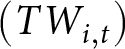 $\left( {T{W_{i,t}}} \right)$, consumption activities $T{Z_{i,t}}$, health maintenance (exercise/prevention, $T{H_{i,t}}$) and illness (treatment, $T{M_{i,t}}$) as follows:
 \begin{equation*}T{A_i} = T{W_{i,t}} + T{Z_{i,t}} + T{H_{i,t}} + T{M_{i,t}}.\end{equation*}
 Changes in fitness levels are redistributed across these time bins, and in particular, increases in  $H$ generally reduce $T{M_{i,t}}$.
2.3. Production
The output and health evolution of the composite product are
 \begin{equation*}{Z_{i,t}}{\text{ }} = Z{\text{ }}\left( {T{Z_{i,t}},{J_{i,t}}} \right);{\text{ }}{H_{i,t}}{\text{ }} = {\text{ }}H\left( {{H_{i,t - 1}},T{H_{i,t}},{M_{i,t}}} \right)\end{equation*}
where  ${J_{i,t}}$ is the market commodity and ${M_{i,t}}$ is the medical input.
2.4. Income
Labour income,  ${Y_{i,t}} = {W_{i,t}} \times T{W_{i,t}}$, satisfies
 \begin{equation*}{Y_{i,t}}{\text{ }} = {W_{i,t}}{\text{ }} \times T{W_{i,t}}{\text{ }} \geqslant {P_j}_{i,t}{\text{ }} \times {J_{i,t}} + {P_m}_{i,t}{\text{ }} \times {M_{i,t}}.\end{equation*}
 Time and budget coupling: health decline increases  $T{M_{i,t}}$, which in turn squeezes out $T{W_{i,t}}$, thereby reducing ${Y_{i,t}}$, which in turn compresses the feasible level of ${J_{i,t}}$, ${M_{i,t}}$.
2.5. Medical treatment time
Medical time  $T{M_{i,t}}$ decreases with health: $\partial TM/\partial H \lt 0$, and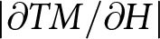 $\left| {\partial TM/\partial H} \right|$ decreases as health improves $\left( {{\partial ^2}TM/\partial {H^2} \gt 0} \right)$. When $H$ approaches the threshold ${H_{{\text{min}}}},{\text{ }}TM \to TA$. This ‘disease avoidance function’ (in Appendix Figure A1) reflects the diminishing returns of time savings from improved health.
2.6. Production possibilities frontier
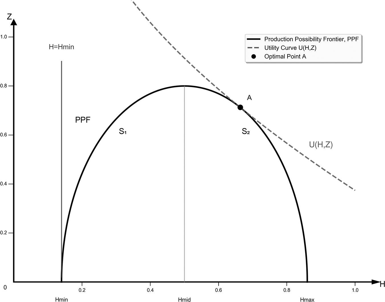
Limited time and income lead to a production possibility frontier (PPF) for ( $H,{\text{ }}Z$), shown in Figure 1. In this framework, extremely poor health (close to ${H_{{\text{min}}}}$) results in all resources being invested in treatment, resulting in $Z \to 0$; while investing almost all resources in health also suppresses $Z$. There is a ‘free lunch’ period (S1): additional health investment simultaneously frees up treatment time, causing ( $H,{\text{ }}Z$) to rise jointly. This period then enters a ‘trade-off’ period (S2), where trade-offs are necessary.
Production possibility frontier.
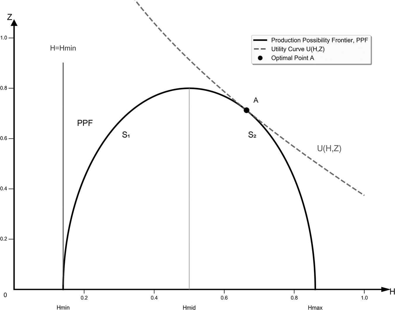
Figure 1 Long description
The graph shows a production possibility frontier labeled PPF, with the x-axis labeled H and the y-axis labeled Z. The curve starts at H equals H subscript min and rises to a peak at S subscript 1, then descends to S subscript 2. A dashed line represents the utility curve U(H,Z), intersecting the PPF at point A, marked as the optimal point. The axes range from 0 to 1, with specific points labeled H subscript min, H subscript mid and H subscript max. The graph includes a legend indicating the production possibility frontier, utility curve and optimal point A.
2.7. Considering air pollution and governance
Incorporating external pollution  ${P_t}$ and governance intensity ${\text{AP}}{{\text{G}}_t}$ into health evolution yields:
 \begin{equation*}{H_{i,t}}{\text{ }} = H\left( {{H_{i,t - 1}},T{H_{i,t}},{M_{i,t}},{P_t},AP{G_t}}\,\right)\!,\end{equation*}
where, assume that  ${\partial }H/\partial{P_t}\, \lt \, 0, {\partial}H/\partial \text{APG}_{t}\, \gt \,0$ and ${\partial ^2}H/\partial {P_t}AP{G_t}\, \gt \,0{\text{ }}$ (governance weakens pollution shocks).
2.8. Model definitions
To facilitate empirical connections, the following reduced time function is used:
 \begin{equation}T{Z_{i,t}} = {Y_{i,t}}^\alpha + {H_{i,t}}^\beta \end{equation}
 \begin{equation}T{H_{i,t}} = {H_{i,t}}^{ - \gamma }\end{equation}
 \begin{equation}T{M_{i,t}} = {\left( {{H_{i,t}} - {H_{min}}} \right)^{ - \delta }},\end{equation}
 where parameters  $\alpha ,{\text{ }}\beta ,{\text{ }}\gamma ,{\text{ }}\delta \gt 1$ (guaranteed first-order direction and second-order curvature assumptions).
The health evolution equation simplifies to:
 \begin{equation}{H_{i,t}}{\text{ }} = {H_{i,t - 1}} + T{H_{i,t}}^\eta + {M_{i,t}}^\theta - {\text{APG}_t}^{ - \mu }{P_t}^\rho \end{equation}
where  $0 \lt \eta ,\theta ,\mu \lt 1,{\text{ }}\rho \gt 1$. Therefore, $\partial H/\partial {\text{AP}}{{\text{G}}_t} = \mu \gt 0$, and at high pollution levels (large $\rho {P_t}$), the ‘net improvement’ of governance is more marginal.
2.9. Health effects of APG
Find the partial derivative of Equation (4):
 \begin{equation*}\frac{{\partial {H_{i,t}}}}{{\partial {\text{AP}}{{\text{G}}_t}}} = \mu {\text{AP}}{{\text{G}}_t}^{ - {\mu } - {\text{1}}}{P_t}^{\rho } \gt 0.\end{equation*}
 If the nonlinear damage of pollution is explicitly written as  $f({P_t}$) with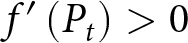 $f'\left( {{P_t}} \right) \gt 0$,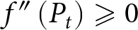 $f''\left( {{P_t}} \right) \geqslant 0$ and the treatment is set to reduce the ‘effective pollution’ $\tilde P = {P_t}\cdot g\left( {\text{APG}_t} \right),$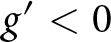 $g' \lt 0$, then $\partial H/\partial {\text{AP}}{{\text{G}}_t} = \mu - f'\left( {{P_t}} \right){P_t}g'\left( {{\text{AP}}{{\text{G}}_t}} \right) \gt 0$, and this term is larger in the high value area of ${P_t}$.
Proposition 1 (Heterogeneity in health improvement): For those with lower initial health or income, (i) the proportion of treatment time is high, and (ii) the ability to avoid or invest in self-protection is low, such that the reduced ‘effective exposure’ from governance leads to a greater net increase in health, so  $\partial {H_{{\text{low}}}}/\partial {\text{APG}} \geqslant \partial {H_{{\text{high}}}}/\partial {\text{APG}}$.
Hypothesis I: Air pollution governance may improve health.
2.10. Income inequality mitigation
Equations (1)–(4) show the marginal transmission of available health improvements to income:
 \begin{equation*}\frac{{\partial {{Y}_{i,t}}}}{{\partial {{H}_{{\text{i,t}}}}}}{\text{ = }\omega \Phi }\left( {{{H}_{{i,t}}}{, \gamma , \delta , \beta }} \right) \quad\text{and}\quad \frac{{\partial {Y_{i,t}}}}{{\partial {\text{AP}}{{\text{G}}_t}}}{\text{ = }}\frac{{\partial {Y_{i,t}}}}{{\partial {H_{i,t}}}}{\text{ \times }}\frac{{\partial {H_{i,t}}}}{{\partial {\text{AP}}{{\text{G}}_t}}} \gt 0\end{equation*}
 Since  $\alpha \gt 1$, the marginal income increase of high-income earners is less sensitive to governance; consequently, governance relatively increases the income growth rate of low-income earners.
Proposition 2 (Easing income inequality): If the marginal contribution of health to productivity decreases (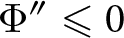 $\Phi '' \leqslant 0$) and Proposition 1 holds, then ${\Delta }Y = {Y_{{\text{high}}}} - {Y_{{\text{low}}}}$ decreases as ${\text{AP}}{{\text{G}}_t}$ increases.
Hypothesis II: Air pollution governance reduces income inequality by improving health.
3. Data and variables
3.1. Data
We use micro-level data from the China Health and Nutrition Survey (CHNS), an on-going multiwave open cohort jointly administered by the University of North Carolina at Chapel Hill and the Chinese Center for Disease Control and Prevention. The survey follows roughly 7,200 households in 15 provinces exhibiting broad variation in geography, economic development, public resources and health status. Waves were fielded in 1989, 1991, 1993, 1997, 2000, 2004, 2006, 2009, 2011 and 2015. Because the indicators required to construct APG measures are available only after 2003, we use the 2004, 2006, 2009, 2011 and 2015 waves. Focusing on health, income inequality and associated welfare effects, we restrict the sample to adults aged 18–64 years. The final dataset comprises 11,050 individual observations across 5 waves, spanning 39 prefecture-level jurisdictions, 167 communities (villages or urban streets) and 4,562 households.
3.2. Description of variables
3.2.1. Individual health (Disease)
Following Fan et al. (Reference Fan, He and Zhou2020), we use the CHNS item: ‘Have you had any of the following symptoms in the past four weeks (including today)?’ Categories: fever/sore throat/cough; diarrhoea; stomach ache; asthma; headache/dizziness; joint or muscle pain; rash/dermatitis; eye or ear disease; heart disease or chest pain; other infectious disease; other non-communicable diseases. Overall, 18.5 per cent reported at least one condition. For robustness, we construct two proxies: (i) Health capital, an entropy-weighted composite of the above categories (indicator weights reported below); and (ii) disease burden count, the cumulative number of distinct reported illness types per individual. These alternative measures test the sensitivity of baseline results to the binary morbidity indicator.
3.2.2. Air pollution governance
Guided by the State Council's 13th Five-Year Plan for ecological and environmental protection, which set binding targets for coal-fired desulphurization and industrial particulate abatement, we measure APG using three city-level indicators: (i) Sulphur dioxide removal rate (SDRR); (ii) industrial smoke (dust) removal rate (ISDR), reflecting end-of-pipe control efficiency in major stationary sources and (iii) PM2.5 attainment rate (PMR), defined as the proportion of monitored days with 24-hour average PM2.5 concentrations at or below the national Grade II standard (75 μg/m3). Incorporating PMR captures policy emphasis on ambient fine particulate outcomes and their documented implications for health, distributional exposure and welfare effects (Chen et al., Reference Chen, Oliva and Zhang2024; Sparks et al., Reference Sparks, Farahbakhsh, Anand, Bauch, Conlon, East, Li, Lickley, Garcia-Menendez, Monier and Saari2024; He et al., Reference He, Pan and Tanaka2025). The trio differentiates engineered abatement performance (SDRR, ISDR) from realized ambient air quality (PMR).Footnote 3
3.2.3. Instrumental variables
We employ two variables for Instrumental variable (IV) of APG: (i) The air circulation coefficient (ACC = wind speed × boundary layer height; Mark, Reference Mark2002) from ECMWF reanalysis; and (ii) the logged frequency of environmental protection words (FEPW) in annual prefecture government work reports (Yang et al., Reference Yang, Huang, Westervelt, Horowitz and Peng2022). ACC captures exogenous atmospheric dispersion capacity that facilitates compliance and strengthens governance intensity while remaining plausibly orthogonal to contemporaneous health after controls. The textual salience measure reflects ex ante policy prioritization: reports are issued early each year, shaping administrative effort but not directly influencing health, income inequality, or welfare effects except through APG. Relevance arises because greater dispersion and higher policy salience incentivize stricter enforcement; exclusion rests on the absence of independent pathways from meteorological dispersion or document wording to outcome variables beyond the governance channel.
3.2.4. Control variables (Controls)
At the individual level, we control for age, gender, educational attainment, urban/rural locality and marital status. At the city level, we include indicators of economic development, health care capacity and demographic scale: GDP, number of hospitals and number of doctors (standardized by population where indicated). Descriptive statistics for all variables appear in Appendix Table A1.
4. Health effects
4.1. Analytical model
The theoretical framework links APG to health and income inequality, supporting Hypotheses I–II. To empirically test Hypothesis I, we estimate the following econometric model:
 \begin{equation}
Disease_{i,j,t} = \alpha + \beta \text{APG}_{i,j,t} + \sum_k {\delta _k}{X_k} + ind{\lambda _i} + {year_t} + {city_t} + {\varepsilon _{i,j,t}}.\end{equation}
\begin{equation}
Disease_{i,j,t} = \alpha + \beta \text{APG}_{i,j,t} + \sum_k {\delta _k}{X_k} + ind{\lambda _i} + {year_t} + {city_t} + {\varepsilon _{i,j,t}}.\end{equation} 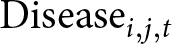 ${\text{Diseas}}{{\text{e}}_{i,j,t}}$ is a binary morbidity indicator (health).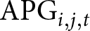 ${\text{AP}}{{\text{G}}_{i,j,t}}$ measures city-level APG intensity (main explanatory variable). ${X_{i,j,t}}$ denote individual and city controls. Indices $i,{\text{ }}j,{\text{ }}t$ refer to individual, city and year, respectively. ${ind}_{i}$, ${year}_{t}$ and ${city}_{i}$ are individual, year and city fixed effects, respectively. ${{\varepsilon }_{{\text{i,j,t}}}}$ is the idiosyncratic error term.
Because the dependent variable (Disease) is binary, linear panel models provide average marginal effects but mask the nonlinear change in illness probability. To quantify how APG alters the likelihood of morbidity (health), we estimate a fixed-effects logit model (conditional on individual or city effects), specified as:
 \begin{equation*}{\text{ln}}\left[ {\frac{{{\text{P(Disease = 1}}{{\text{)}}_{{\text{i,j,t}}}}}}{{{\text{1 - P(Disease = 1}}{{\text{)}}_{{\text{i,j,t}}}}}}} \right]{ = \alpha + \beta\,}{{\text{APG}}_{{\text{i,j,t}}}}{\text{ + }}\sum_{\text{k}} {{\delta }_{\text{k}}}{{\text{X}}_{\text{k}}} + {ind}_{i} + {year}_{t} + {city}_{t}{\text{ + }}{{\varepsilon }_{i,j,t}},\end{equation*}
where  $P$ is the probability of an individual having the disease and the rest of the variables are consistent with the definitions above.
4.2. Baseline results
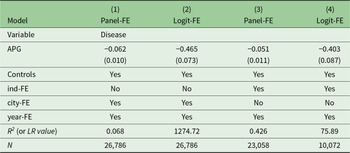
Table 1 reports the association between APG and health. All four specifications include individual and city controls plus year fixed effects. Columns (1)–(2) adopt city fixed effects; columns (3)–(4) adopt individual fixed effects. Columns (1) and (3) use linear panel FE (Panel-FE); columns (2) and (4) use fixed-effects logit (Logit-FE).
Baseline results
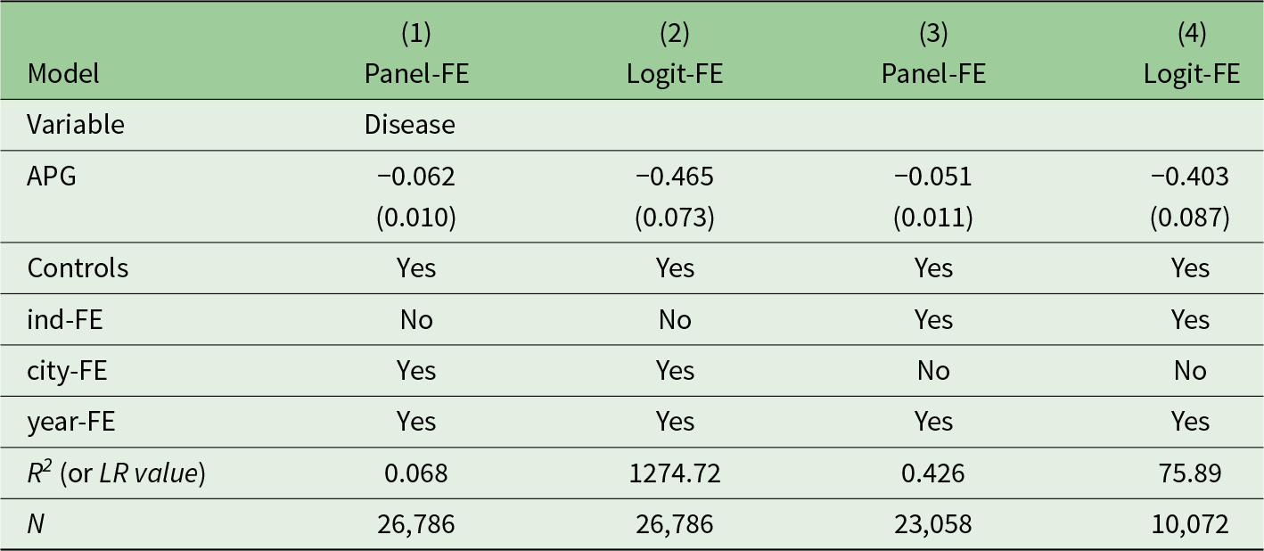
Table 1 Long description
The table compares the effects of APG on disease across four models, two Panel-FE and two Logit-FE, with varying fixed effects and sample sizes. The APG coefficient is negative in all models, indicating a potential reduction in disease with increased APG. The Panel-FE models show smaller negative coefficients for APG compared to the Logit-FE models. The R-squared value is higher in the second Panel-FE model, suggesting a better fit compared to the first. The sample sizes differ, with the Panel-FE models having larger samples than the Logit-FE models. The presence of individual and city fixed effects varies across models, which may influence the results. The interpretation of these results should consider the exclusion of certain variables in the Logit-FE models.
Notes: Standard error statistics are in parentheses. According to the statistical results in Appendix Table A1, the mean value of APG is 1.073. Therefore, increasing APG by one unit is equivalent to doubling the governance strength of the region. In the Logit-FE regression model, the presence of the explanatory variable (presence of illness) was not considered for inclusion in the regression analyses if the individual did not change, so the sample size was not consistent with the sample size of the Panel-FE regression model results.
Across both Panel-FE specifications (with city and with individual fixed effects), APG exhibits a consistently negative and statistically significant association with health risk: stronger governance corresponds to a lower incidence of reported illness. The Logit-FE estimates likewise yield a large and significant effect; the implied economic magnitude indicates that a doubling (1 unit increase) in APG reduces the average probability of illness by 40.3 per cent, evidencing substantial welfare effects alongside potential mitigation of income inequality in health outcomes.
4.3. Addressing endogeneity
This section evaluates how APG affects health while confronting identification challenges. First, reverse causality: governance is a prefecture-level (macro) construct, whereas health is individual (micro), making feedback less direct. Yet aggregate health shapes human capital, which can influence growth, emissions and subsequent governance, hence residual reverse linkage cannot be ignored. Second, measurement error: individual morbidity in the CHNS may suffer from recall bias or under-registration. Third, omitted variables: despite rich individual and city controls, unobserved factors (e.g., behavioural risks, informal care access) may bias estimates.
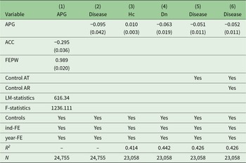
To address endogeneity, we instrument APG with the ACC and the logged FEPW using two-stage least squares. Table 2, columns (1)–(2), reports results. First-stage estimates show both instruments strongly predict governance intensity. Second-stage coefficients confirm that stronger APG lowers the probability of illness, closely matching baseline magnitudes. Kleibergen–Paap LM and Wald F statistics reject the under-identification and weak instrument hypotheses, supporting instrument validity. Thus, the causal effect on health remains robust after correcting for endogeneity, reinforcing associated welfare effects and the potential pathway to reduced health-related income inequality.
Endogeneity and robustness tests
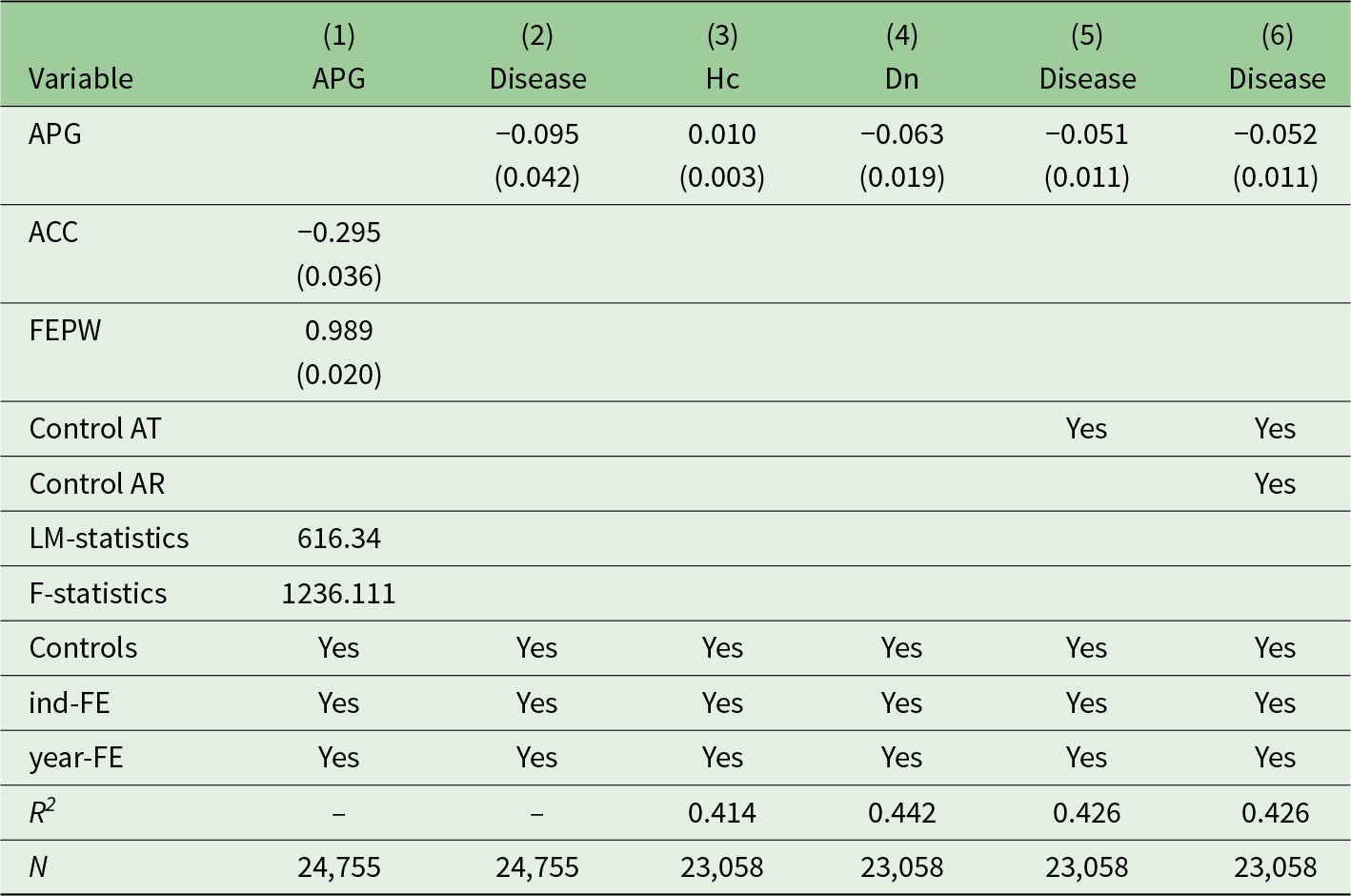
Table 2 Long description
The table examines the relationship between various variables such as APG, Disease, and others, with a focus on endogeneity and robustness. APG has a negative effect on Disease in columns 2, 5, and 6, with coefficients of -0.095, -0.051, and -0.052, respectively, indicating a consistent negative relationship. FEPW shows a strong positive effect on APG with a coefficient of 0.989. Control variables for average temperature and rainfall are included in some columns, specifically columns 5 and 6. The R-squared values in columns 3 to 6 range from 0.414 to 0.442, suggesting moderate explanatory power. The number of observations is consistent across columns 3 to 6, with 23,058 observations each. The table includes controls for individual and year fixed effects across all columns.
Notes: Standard error statistics are in parentheses. AT is average temperature and AR is average rainfall of city.
To ensure the reliability of our IV analysis, we conduct an additional robustness check using the lagged FEPWs as an alternative instrument. This specification addresses potential concerns about implementation lags between governance decisions and their actual effects. The results remain highly consistent with our main findings, with strong first-stage predictions and second-stage coefficients that closely align with baseline estimates (Appendix Table A2).
4.4. Robustness test
Beyond addressing endogeneity (model substitution and IVs), potential selection bias remains if health is proxied only by a binary sickness indicator. To broaden measurement, we construct two complementary outcomes. (i) Health capital (Hc): using the entropy weight method, we integrate multiple disease indicators (all treated as negative attributes; Appendix Table A3 reports variables and weights). Higher Hc denotes greater latent health stock. (ii) Total number of diseases (Dn): the summed self-reported conditions from the questionnaire; higher Dn implies poorer health. In Table 2, robustness results (columns (3)–(4)) show that APG significantly increases Hc and, consistently, reduces Dn. These effects mirror baseline economic magnitudes, reinforcing that APG improves health.
Furthermore, following established practices in air pollution health studies (Neidell, Reference Neidell2004; Xia et al., Reference Xia, Xing, Xu and Pan2022), we progressively incorporate regional weather controls, specifically average temperature and rainfall from satellite imagery, which might confound the governance–health relationship. The consistency of coefficients across these specifications (Table 2, columns (5)–(6)) demonstrates that our findings remain robust when accounting for meteorological factors that could influence both pollution dispersion and health outcomes directly.
5. Income effects
5.1. Gini index
The Gini index is a standard metric of income inequality (Gastwirth, Reference Gastwirth1972). To test Hypothesis II, we assess the relation between APG and income inequality using the Gini index. For each year, prefectures are split at the annual median of the governance measure into stronger and weaker governance groups, producing eight year-specific data groups. We then compute the Gini index separately for each group to compare distributional outcomes under differing governance intensities.
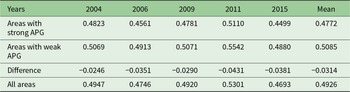
Table 3 shows that regions with stronger APG exhibit systematically lower Gini coefficients than contemporaneous weaker-governance regions; five-year averages reinforce this pattern, indicating a robust negative cross-sectional association between governance intensity and income inequality. However, this correlation alone does not warrant a causal claim that effective governance has unambiguously alleviated regional economic disparity. A substantial literature documents channels through which income inequality can shape environmental outcomes: via heterogeneous preferences, political influence, collective action capacity and public goods provision – implying possible reverse causality from distributional structure to governance (Berthe and Elie, Reference Berthe and Elie2015; Liu et al., Reference Liu, Wang, Zhang and Li2018). Thus, the observed gap may reflect (i) a governance-to-inequality pathway (pollution abatement improves health and human capital, narrowing income dispersion); (ii) an inequality-to-governance pathway (more equitable regions mobilize fiscal and regulatory support for stringent governance); and/or (iii) common latent determinants (institutional quality, developmental stage) jointly influencing both variables. Recognizing these identification challenges, subsequent empirical strategies seek to isolate the causal contribution of APG to income inequality.
Trends in the Gini index
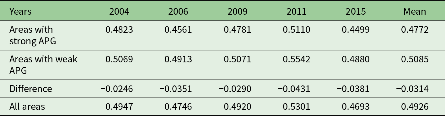
Table 3 Long description
The table measures the Gini index trends from 2004 to 2015 across areas with strong and weak APG, and all areas combined. Areas with weak APG consistently show higher Gini index values compared to areas with strong APG, indicating greater income inequality. The largest disparity between these areas occurred in 2011, with a difference of 0.0431. The mean Gini index for areas with strong APG is 0.4772, while for areas with weak APG, it is 0.5085, further highlighting the inequality gap. All areas combined have a mean Gini index of 0.4926, suggesting a moderate level of inequality overall. These trends suggest that areas with weak APG may require targeted interventions to reduce income inequality.
5.2. Lorenz curve
To provide a more intuitive illustration of how APG relates to income distribution, we plot annual Lorenz curves for the five sample periods. Every year, the curve for regions with stronger APG lies uniformly closer to the 45-degree egalitarian line and thus above the curve for weaker governance regions, implying lower contemporaneous income dispersion where governance is stronger. This graphical evidence is consistent with the negative association between governance intensity and the Gini index, while not itself establishing causality (see Appendix Figures A2–A6).
5.3. Deprivation index
To further assess whether APG is associated with a mitigation of income inequality, we complement the Gini coefficient with relative deprivation metrics. The Gini index, while standard, has notable limitations for our purposes. (i) It yields a single aggregate snapshot, masking how inequality is experienced across individuals and income tiers; it is insensitive to the distribution of shortfalls faced by specific subgroups. (ii) it offers limited dynamic diagnostic power: changes in the Gini index cannot be decomposed to reveal contribution channels or the trajectory of different quantiles, risking under-attention to low-income groups’ welfare losses or high-income groups’ relative positional gains.
Accordingly, after documenting Gini patterns, we employ three widely used relative deprivation indices, the Yitzhaki (Reference Yitzhaki1979), Kakwani (Reference Kakwani1984) and Podder (Reference Podder1996) measures, to triangulate the relationship between governance intensity and distributional outcomes. The Yitzhaki index treats an individual's deprivation as the aggregate income gap vis-à-vis all richer peers and can be interpreted as a component (or re-expression) of the absolute Gini. The Kakwani index rescales Yitzhaki by the group mean to reduce sensitivity to absolute income size and shares the same mean value as the Gini, thereby preserving comparability (Lhila and Simon, Reference Lhila and Simon2010; Adjaye-Gbewonyo and Kawachi, Reference Adjaye-Gbewonyo and Kawachi2012). The Podder index (logarithmic form) addresses the dependence of Yitzhaki on the range and mean by assuming (in its derivation) an underlying parametric form, yielding a measure less affected by scale shifts (Podder, Reference Podder1996). Using these complementary metrics allows us to test whether results hinge on a single scalar of inequality or extend to perceived relative shortfalls, a dimension closely tied to welfare effects.
Table 4 reports estimates with each deprivation index as the dependent variable. Across specifications (columns (1)–(3)), stronger APG is associated with significantly lower Yitzhaki, Kakwani and Podder values. The consistent negative coefficients reinforce the baseline evidence that governance intensity correlates with reduced relative deprivation and narrower income inequality.
Other income inequality indices
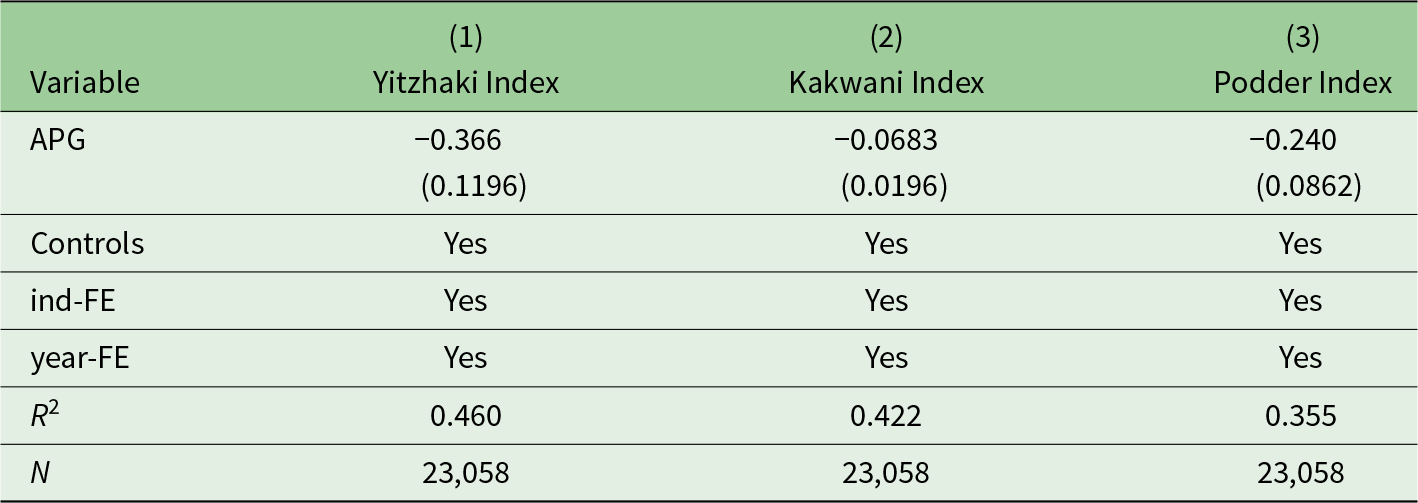
Table 4 Long description
The table compares three income inequality indices: Yitzhaki, Kakwani, and Podder, in relation to the variable APG. The Yitzhaki-index has the strongest negative association with APG at -0.366, followed by the Podder-index at -0.240, and the Kakwani-index at -0.0683. Each index includes controls and fixed effects for individual and year, ensuring consistency across the data. The R-squared values indicate the proportion of variance explained by the model, with the Yitzhaki-index at 0.460, Kakwani-index at 0.422, and Podder-index at 0.355. All indices are based on a sample size of 23,058 observations. Standard errors are provided in parentheses, suggesting variability in the estimates.
Note: Standard error statistics are in parentheses.
5.4. Income effects in different groups
5.4.1. Analytical econometric models
Guided by the theoretical model, we test whether the income effect of APG varies across the income distribution. We implement heterogeneity analyses by partitioning the sample into two, three and four quantile groups, emphasizing differential impacts on the low-income segment and benchmarking against full-sample estimates. We intentionally employ income group stratification rather than an IV design: treating APG as an instrument for health would violate the exclusion restriction because governance can directly alter income via plant closures, technology upgrading, compliance cost pass-through, labour reallocation and productivity restructuring. Using Mobarak's (Reference Mobarak2005) style linkage equations, we then examine whether incremental income gains operate through health, illuminating the mechanism through which governance contributes to reduced income inequality:
 \begin{equation}{\text{ }}Incom{e_{i,j,t}}{\text{ }} = {\alpha _0} + {\alpha _1}Diseas{e_{i,j,t}}{\text{ }} + {\alpha _2}{\text{APG}_{i,j,t}}{\text{ }} + \sum_{k} {\delta _k}{X_k} + ind{\lambda _i}{\text{ }} + yea{r_t}{\text{ }} + {\varepsilon _{i,j,t}}\end{equation}
 \begin{equation}{\text{ }}Diseas{e_{i,j,t}}{\text{ }} = \alpha + {\beta _1}\text{APG}_{i,j,t}{\text{ }} + \sum_k {\delta _k}{X_k} + ind{\lambda _i} + yea{r_t}{\text{ }} + {\varepsilon _{i,j,t{\text{ }}}},\end{equation}
 where income denotes monthly earnings from regular employment. Equation (6) estimates the income equation, jointly identifying the direct impact of APG  $\left( {{\alpha _2}} \right)$ and health. Equation (7), structurally aligned with Equation (5), models health as a function of APG $\left( {{\beta _1}} \right)$. The mediated (indirect) income effect of governance through health is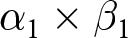 ${\alpha _1} \times {\beta _1}$, where ${\alpha _1}$ is the return of health in the income equation. Thus, the total effect on individual income is ${\alpha _2} + {\alpha _1} \times {\beta _1}$, decomposed into direct $\left( {{\alpha _2}} \right)$ and indirect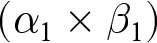 $\left( {{\alpha _1} \times {\beta _1}} \right)$, components relevant to income inequality and broader welfare effects.
5.4.2. Grouped by income
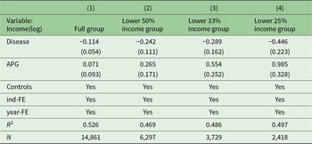
The results in Table 5, across progressively poorer subsamples, show that the Disease variable exhibits increasingly negative income effects: the fixed-effects estimates are −0.114 for the full sample, −0.242 for the bottom 50 per cent, −0.289 for the bottom 33 per cent and −0.446 for the bottom 25 per cent (generally statistically significant), indicating that adverse health shocks impose a markedly steeper earnings penalty on low-income individuals, consistent with weaker access to formal job protection or compensatory assets and thus a health-driven amplification of lower-tail inequality. In contrast, APG shows a monotonic increase in its positive association with income −0.071 in the full sample, 0.265 for the bottom half, 0.554 for the bottom third and 0.985 for the poorest quarter-shifting from negligible or marginal precision in the broader sample to economic and statistical significance in the lower strata. This gradient implies that governance interventions disproportionately raise earnings at the bottom, plausibly through localized employment generated by abatement and enforcement activities, reductions in pollution-related work interruptions, or reallocation toward cleaner, more labour-absorptive sectors. Taken together, deteriorating health conditions deepen income disparities, while enhanced environmental governance exerts a progressive (inequality-mitigating) effect by delivering larger proportional gains to the poorest workers.
Changes in the incomes of different groups
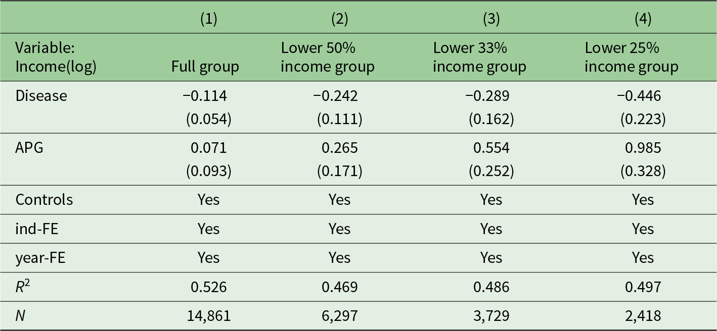
Table 5 Long description
The table examines the impact of disease and APG on income across different income groups, specifically the full group, lower 50%, lower 33%, and lower 25% income groups. Disease negatively affects income, with the most substantial decrease observed in the lower 25% income group, where income reduces by 0.446. Conversely, APG positively influences income, with the largest increase also seen in the lower 25% group, at 0.985. All groups have controls, individual fixed effects, and year fixed effects applied. The R-squared values range from 0.469 to 0.526, indicating varying degrees of model fit across groups. The sample sizes differ significantly, with the full group having 14,861 observations and the lower 25% group having 2,418.
Note: Standard error statistics are in parentheses.
A residual concern is reverse causality: income changes may subsequently influence individual health (through medical access, nutrition, or exit from risky jobs) and the intensity of local APG (via greater fiscal capacity, community demand, or, conversely, targeted support to poorer areas). Such pathways could modestly attenuate or amplify the estimated gradients, although individual and year fixed effects already absorb time-invariant heterogeneity and common shocks. For robustness, replacing contemporaneous APG with its one-period lag also yields qualitatively and quantitatively similar coefficients across all income strata, suggesting that possible reverse causation issues are unlikely to overturn the above results.
5.4.3. Grouped by area
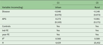
Following epidemiological literature highlighting spatial disparities in health determinants (Rodgers, Reference Rodgers1979; Kawachi and Kennedy, Reference Kawachi and Kennedy1999; Subramanian and Kawachi, Reference Subramanian and Kawachi2004), we examine urban–rural heterogeneity in the health-income relationship. Table 6 presents disaggregated estimates across settlement types. The results reveal that disease incidence has a substantially larger negative effect on income in rural areas (−0.148) compared to urban areas (−0.040), although the urban coefficient is statistically insignificant. Similarly, APG exhibits heterogeneous effects − positive in urban areas but negative in rural regions, albeit neither coefficient achieves statistical significance. These patterns suggest that the health-income gradient may be steeper in rural China, potentially reflecting differential access to healthcare resources, insurance coverage and income diversification opportunities between urban and rural populations.
Urban–rural heterogeneity
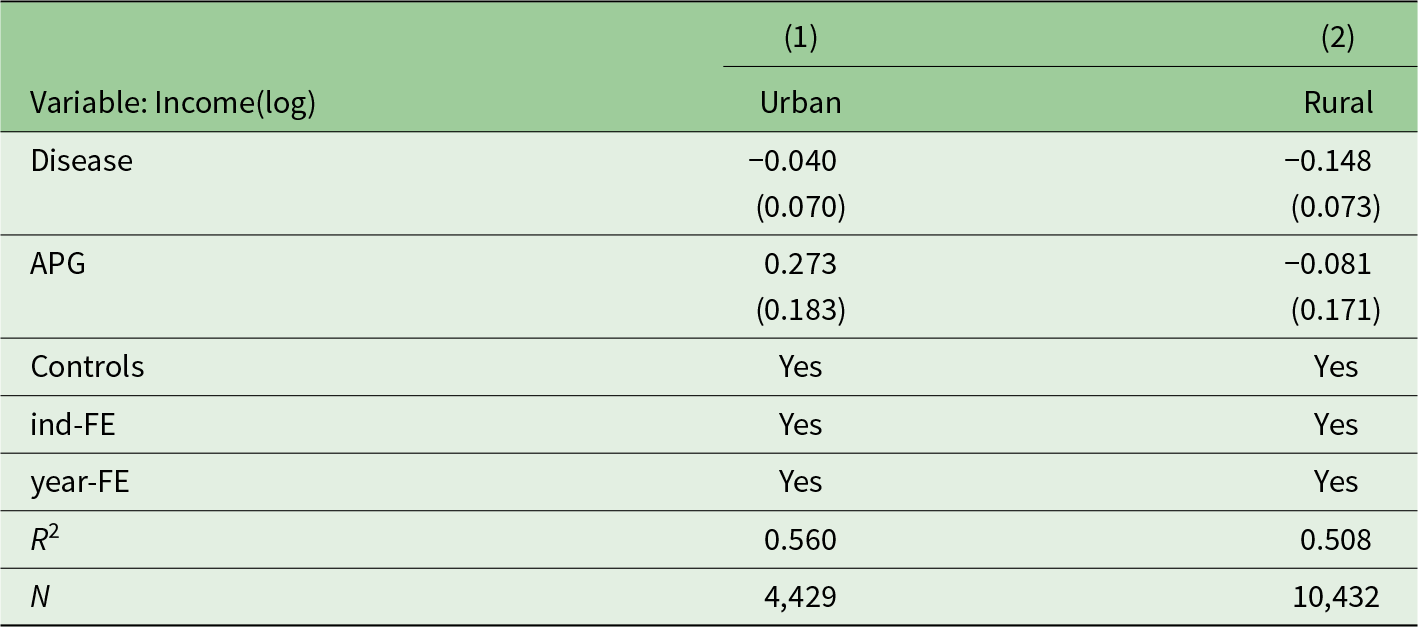
Table 6 Long description
The table compares the impact of income on disease and APG in urban and rural settings. In rural areas, income is more negatively associated with disease than in urban areas, with coefficients of -0.148 and -0.040 respectively. Conversely, urban areas show a stronger positive association with APG, with a coefficient of 0.273 compared to -0.081 in rural areas. Both settings include controls, individual fixed effects, and year fixed effects. The R-squared values indicate that the model explains 56% of the variance in urban areas and 50.8% in rural areas. The sample sizes are 4429 for urban and 10432 for rural areas, suggesting a larger rural sample. Standard errors are provided in parentheses, indicating variability in the estimates.
Note: Standard error statistics are in parentheses.
5.4.4. Total effect
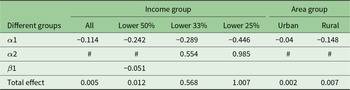
Building on the computational scheme in Equations (6) and (7), the total effect of APG on income can be decomposed into direct and indirect (health-mediated) components across different population segments. Table 7 presents these effects by income quantiles and urban–rural divisions (results with insufficient statistical significance are excluded from calculation). For income groups, we observe a clear pattern: the total effect strengthens monotonically toward poorer strata, from 0.005 for the full sample to 1.007 for the lowest quartile. This gradient provides strong support for Hypothesis II, demonstrating that APG generates disproportionately larger income gains for disadvantaged groups once the mediated health channel is incorporated. The urban–rural decomposition reveals a similar pattern, with rural residents (0.007) experiencing marginally higher total benefits than their urban counterparts (0.002), though this difference is less pronounced than across income quantiles. These findings collectively reinforce our conclusion that environmental governance yields progressive distributional effects through health-income pathways.
Total effect of APG on income in different group
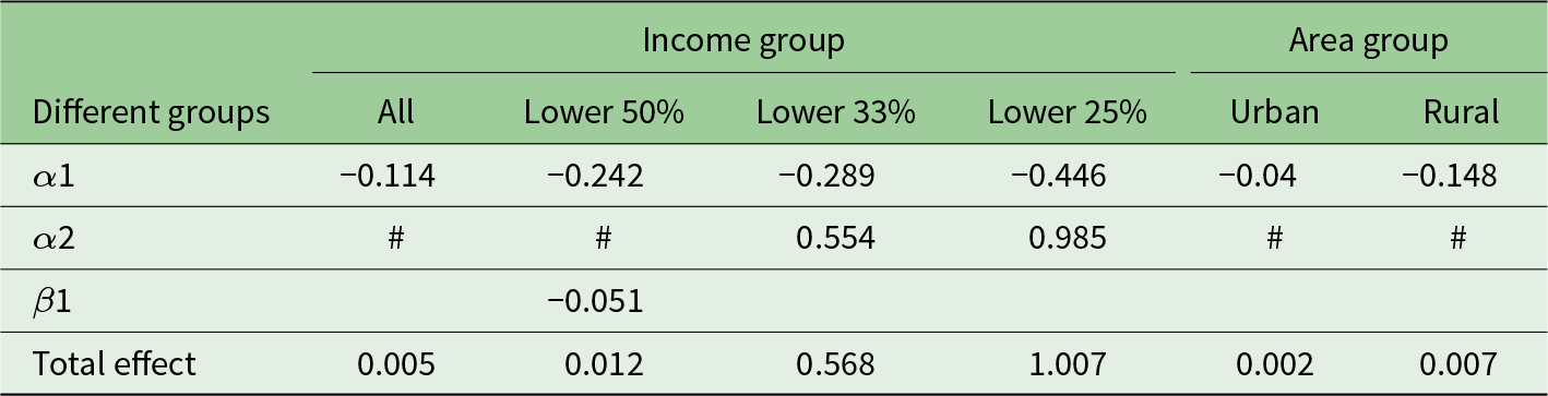
Table 7 Long description
The table measures the total effect of APG on income across different income and area groups. The most significant effect is observed in the lower 25% income group, with a value of 1.007, indicating a strong impact. In contrast, the effect is minimal in urban areas, with a value of 0.002. The lower 33% income group also shows a notable effect of 0.568. The coefficients for some groups are marked as not significant, indicating they are not used in calculations. This suggests variability in the impact of APG across different demographics, with rural areas experiencing a slightly higher effect than urban areas.
Note: # indicates that the coefficient is not significant and is no longer used in the calculation.
6. Welfare effects
The theoretical framework models individuals allocating time to consumption 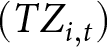 $(T{Z_{i,t}})$ and exercise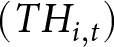 $(T{H_{i,t}})$ and expenditures on market goods $\left( {{J_{i,t}}} \right)$ and medical care $\left( {{M_{i,t}}} \right)$ to produce a composite consumption good $\left( {{Z_{i,t}}} \right)$ and health $\left( {{H_{i,t}}} \right)$, the two arguments of utility. Empirical evidence shows that APG improves health and thereby raises low-income earnings, shifting individual PPFs outward and increasing utility.
6.1. Alterations of PPF
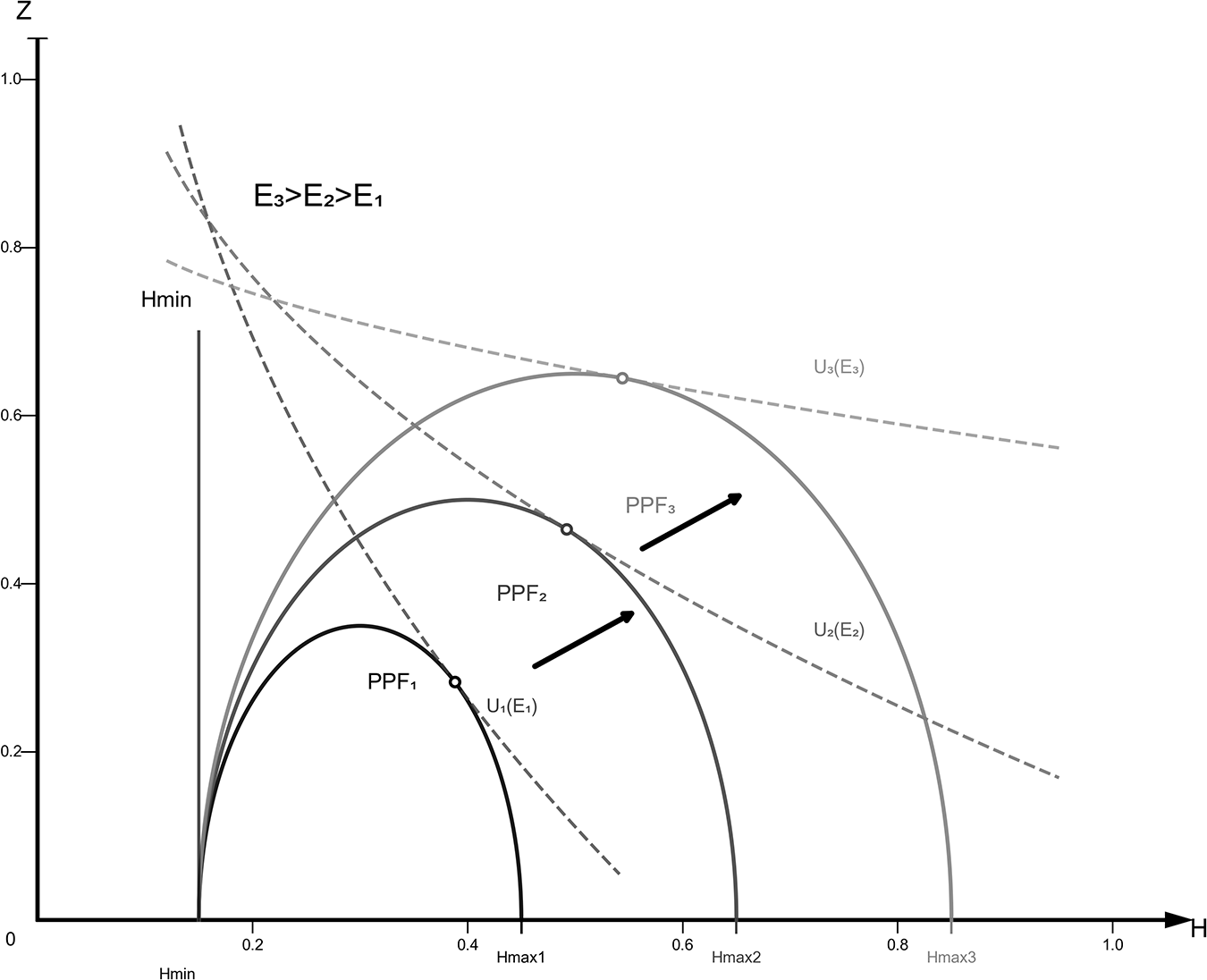
The first step assesses how environmental governance shifts the individual PPF. Prior evidence shows that such governance improves public health and raises consumption, implying an outward (upper-right) shift of the PPF in Figure 2.Footnote 4 While the mortality threshold  ${H_{{\text{min}}}}$ is unchanged, the attainable maxima for health $\left( {{H_{{\text{max}}}}} \right)$ and composite consumption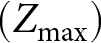 $\left( {{Z_{{\text{max}}}}} \right)$ both rise, moving the optimal production point outward and increasing utility. This expansion enlarges both the previously defined free-lunch zone (outputs attainable without additional individual inputs) and the trade-off region. Under resource scarcity and cognitive constraints, individuals disproportionately operate within the free-lunch zone; governance thus broadens this zone, allowing resource-constrained persons to secure higher health and consumption outcomes without extra private effort or expenditure, thereby enhancing welfare.
Alterations of PPF.
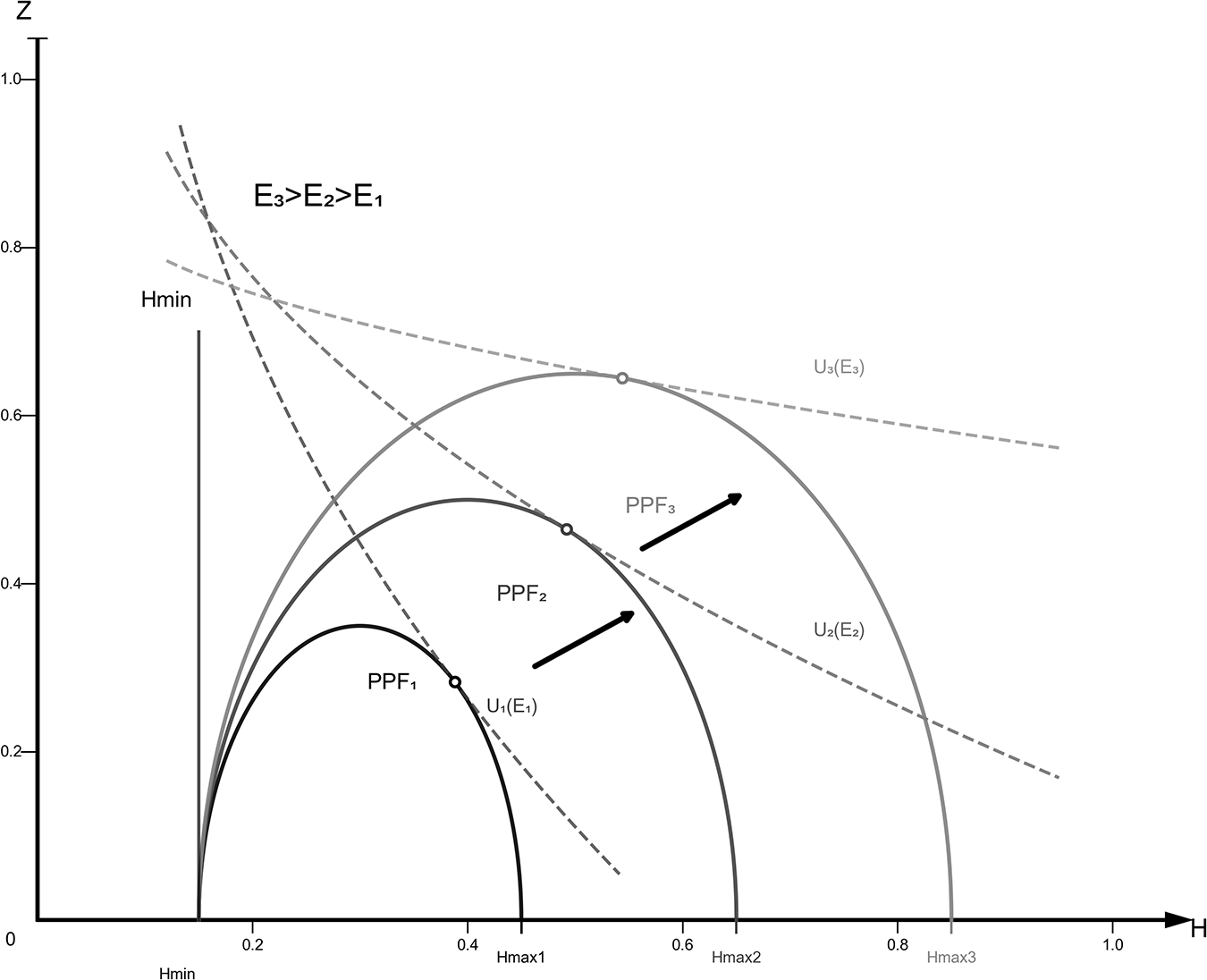
Figure 2 Long description
The graph shows production possibility frontiers labeled PPF subscript F, PPF subscript I and PPF subscript S, each representing different scenarios. The x-axis is labeled 'Health' with units from H subscript min to H subscript max and the y-axis is labeled 'Z' with units from 0 to 1.0. Curves U subscript E subscript F, U subscript E subscript I and U subscript E subscript S represent utility levels. The graph indicates shifts in the PPF, with arrows showing movement from PPF subscript F to PPF subscript I and PPF subscript S, suggesting changes in health and consumption outcomes. The notation E subscript S greater than E subscript F greater than E subscript I is present, indicating comparative efficiency levels.
6.2. Changes in utility
The results above show that environmental governance jointly shifts individual consumption and health, thereby raising utility. We therefore test whether regulation delivers welfare gains by specifying a utility function that is logarithmic in composite consumption  ${Z_{i,t}}$ and linear in health capital ${H_{i,t}}$ above a survival threshold ${H_{{\text{min}}}}$. ${H_{i,t}}{\text{ }}$below ${H_{{\text{min}}}}$ yields no meaningful life utility; above H min, each additional unit of health adds a constant marginal utility. In contrast, consumption displays diminishing marginal utility, consistent with standard preferences. Labour time $l$ exhibits high initial marginal contribution (up to the conventional 8-hour workday, $l$ = 1/3), after which additional hours constitute overtime with sharply declining, eventually near-zero (or negative) marginal utility; empirical behaviours imply an effective upper bound around 16 hours ( $l$ = 2/3). This pattern reflects growing aversion to extended hours and minimal incremental welfare beyond that point. Accordingly, the utility structure can be represented in reduced form as a linear term in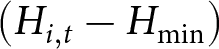 $\left( {{H_{i,t}} - {H_{{\text{min}}}}} \right)$, a logarithmic term in ${Z_{i,t}}$, and a convex disutility (or strongly diminishing marginal benefit) component of labour time capturing overtime penalties:
 \begin{equation*}{\text{ }}{U_{i,t}}{\text{ }} = U{\text{ }}\left( {{H_{i,t}},{Z_{i,t}}} \right) = {\text{ }}ln\left( {{Z_{i,t}}} \right) + {H_{i,t}} - {H^0}_{i,t} - \frac{{{l^{\left( {1 + \rho } \right)/\rho }}}}{{\left( {1 + \rho } \right)/\rho }}\end{equation*}
where  $\rho $ denotes the Frisch labour supply elasticity − the responsiveness of hours to transitory wage changes holding the marginal utility of wealth constant (Martínez et al., Reference Martínez, Saez and Siegenthaler2021). Empirically, $\rho $ lies in [0,1]; recent estimates place it at 0.27–0.53 with a central value of 0.40 (Whalen and Reichling, Reference Whalen and Reichling2017).
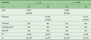
To gauge the sensitivity of welfare valuations to the short-run adjustability of labour supply, we consider two values of the Frisch elasticity parameter  $\rho $. In the benchmark ‘inelastic’ case ( $\rho = 0$), we implement perfectly inelastic labour supply by treating hours $l$ as an exogenously fixed constant $\bar l$; consequently the labour disutility term v(l) =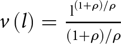 $v\left( l \right) = \frac{{{{\text{l}}^{\left( {{1 + \rho }} \right){/\rho }}}}}{{\left( {{1 + \rho }} \right){/\rho }}}$ becomes a column-specific constant and is omitted from the reported welfare measure. Individual welfare in this case is therefore a function only of consumption (implicit in the composite numeraire) and health capital. In the alternative specification with ρ = 0.40 labour supply is endogenously adjustable; the corresponding labour disutility is $v\left( l \right) = {l^{3.5}}/3.5$, which implies a Frisch (intertemporal) elasticity of 0.40.
We quantify welfare effects by decomposing utility changes into components attributable to APG and to disease, as shown in Table 8. Columns (1)–(2) assume a Frisch labour supply elasticity  $\rho = 0$; columns (3)–(4) impose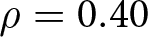 $\rho = 0.40$. In columns (1) and (3), the key regressor is APG; in columns (2) and (4) the key regressor is individual health status (indicator for being sick). When $\rho = 0$, labour supply is perfectly inelastic: wage changes do not alter hours. By construction the labour term ${l^{\left( {1 + \rho } \right)}}/\rho /\left( {1 + \rho {\text{ }}} \right)/\rho {\text{ }}$ drops out, so individual utility depends only on consumption and health. When $\rho $ = 0.40, a 1 per cent transitory wage increase induces a 0.4 per cent increase in supplied hours – hours elasticity equals 0.40. In this calibrated case, the labour component reduces to $\frac{{{l^2}}}{2}$, so utility now reflects consumption, health and the (diminishing) marginal contribution of working time.
Welfare effects of air pollution governance and disease
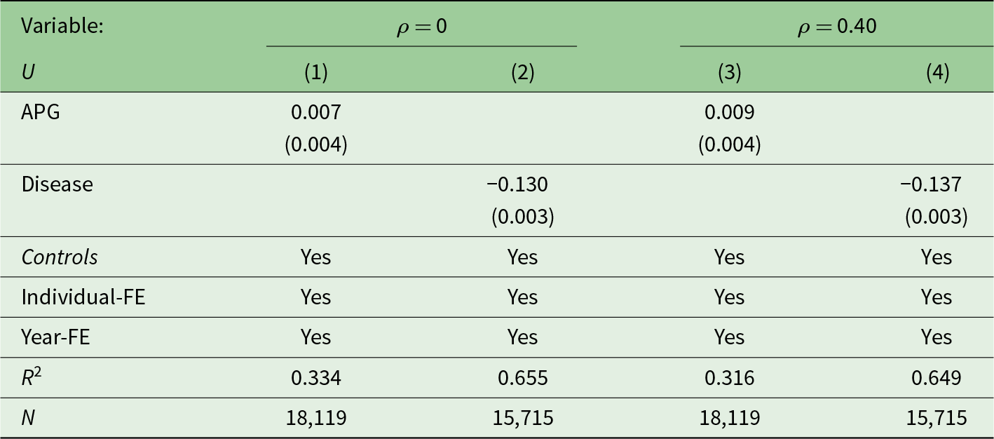
Table 8 Long description
The table examines the welfare effects of air pollution governance and disease on labor time, comparing scenarios with different correlation coefficients. Key findings include a positive impact of air pollution governance on welfare, with coefficients of 0.007 and 0.009 for the scenarios with zero and 0.40 correlation, respectively. Disease has a negative effect, with coefficients of -0.130 and -0.137. The R-squared values indicate a stronger model fit when the correlation is 0.40, with values of 0.655 and 0.649 compared to 0.334 and 0.316 for zero correlation. The sample sizes are 18,119 and 15,715 for the respective scenarios. All models control for individual and year fixed effects, ensuring robustness of the results.
Notes: Standard error statistics are in parentheses. This result is consistent with the results of Hanna and Oliva (Reference Hanna and Oliva2015), whose study showed that reducing pollution increased workers’ working hours by 5%. This paper also provides an empirical analysis of this and demonstrates that environmental governance significantly enhances the labour time of individuals.
Disease enters with a large, precisely estimated negative effect on welfare: −0.130 (standard error: 0.003) under  $\rho = 0$ and −0.137 (standard error: 0.003) when $\rho $ =0.40. The slightly more negative coefficient in the elastic case implies that allowing labour to adjust accentuates the welfare penalty of disease − plausibly because morbidity not only reduces health utility directly but also curtails the capacity to reallocate labour effort in response to shocks. Overall, the comparison across $\rho $ highlights that (i) assuming perfectly inelastic labour supply provides a lower bound on the welfare benefits of APG; and (ii) even a moderate Frisch elasticity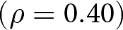 $\left( {\rho = 0.40} \right)$ noticeably magnifies the measured welfare gains while deepening the welfare losses attributable to disease.
7. Conclusion and consequences
Our theoretical framework and empirical evidence show that APG improves health and, through this channel, reduces regional income inequality. These findings are robust to endogeneity corrections and variable-selection concerns. Using the Gini coefficient and relative deprivation indices, we confirm distributional gains: health-mediated income growth among low-income households raises consumption and utility, generating positive welfare effects.
Given evidence that APG reduces income inequality through health gains and generates positive welfare effects, policy should integrate health poverty alleviation and ecological compensation instruments, prioritizing heavily polluted regions and targeted support for low-income households to offset health-related earnings losses. Strengthening institutional linkages among environmental, health and social welfare agencies and deploying green taxes, subsidies and complementary incentives can mobilize firms and citizens while financing equity goals. Establishing a rigorous, long-term monitoring and feedback system will sustain policy effectiveness. Parallel investments in public environmental awareness and health literacy − via curriculum, community outreach and participatory programmes − can entrench a culture of green development. Overall, coordinated APG simultaneously advances ecological quality, social welfare, distributive equity and sustainable development.
Supplementary material
The supplementary material for this article can be found at https://doi.org/10.1017/S1355770X2610059X.
Competing interests
The authors declare none.



 Open access

