


1. Introduction
Turbulent boundary layers are ubiquitous in engineering applications and geophysical flows of interest. A better understanding of turbulent boundary layers will allow for the design of more efficient airplanes, improved wind turbine performance characterisation, and a better understanding of the atmospheric weather patterns that could subsequently inform the prediction and mitigation of wildfire propagation to list only a few examples. These flows have been studied intensely over the past century by both the engineering and geophysical communities. These studies have focused on characterising and quantifying the behaviour of turbulence in the inner and outer regions of the turbulent boundary layers, which has also led to advancements in turbulence models over the years.
The presence of pressure gradients significantly affects the behaviour of a turbulent boundary layer. Adverse pressure gradients (APGs) often precede the onset of turbulent flow separation, which is a major cause of higher aerodynamic drag for wings at high angles of attack. In the presence of a sufficiently strong APG, a flow exhibits an increase in Reynolds shear stresses, often observed as a secondary peak of these quantities in the outer region of the boundary layer. Using the regional similarity hypothesis, Perry, Bell & Joubert (Reference Perry, Bell and Joubert1966) showed that the logarithmic law of the wall for the velocity distribution, hereafter referred to as the log-law, exists in the near-wall region and a half-power law is observed in the transition to the wake region for a boundary layer that is far away from flow separation. These results are also aligned with the asymptotic analysis in Durbin & Belcher (Reference Durbin and Belcher1992), where the role of APGs on a larger wake region was discussed. Marušić & Perry (Reference Marušić and Perry1995) showed that the turbulence intensity in the outer region increases in the presence of an APG when normalised by friction velocity,  $u_{\tau }$. APGs also result in higher turbulence production due to high Reynolds shear stress and dissipation in the outer region of the turbulent boundary layer (Skåre & Krogstad Reference Skåre and Krogstad1994). Conversely, favourable pressure gradients (FPGs) stabilise a boundary layer and reduce turbulence intensity. In the presence of an FPG, a departure from the log-law is commonly observed (Tsuji & Morikawa Reference Tsuji and Morikawa1976; Baskaran, Smits & Joubert Reference Baskaran, Smits and Joubert1987) which can be attributed to an increase in the thickness of the viscous wall region (Narayanan & Ramjee Reference Narayanan and Ramjee1969; Blackwelder & Kovasznay Reference Blackwelder and Kovasznay1972). A reduction in Reynolds stresses, turbulent kinetic energy production and dissipation is commonly observed in the presence of an FPG. A much more significant decrease in production and dissipation of turbulence is observed in the inner region of the boundary layer than in the outer region (Bourassa & Thomas Reference Bourassa and Thomas2009). Strong FPGs can even lead to a reverse transition of a turbulent boundary layer to a laminar state, a process often referred to as relaminarisation. Patel & Head (Reference Patel and Head1968) showed that in the presence of a substantial FPG, even a high-Reynolds-number turbulent boundary layer could relaminarise. This flow behaviour is attributed to a slow response of the boundary layer to the strong FPG. During flow relaminarisation, turbulence still exists in the outer region but has a passive influence on the downstream development of the boundary layer (Launder Reference Launder1964; Jones & Launder Reference Jones and Launder1972) as the pressure forces dominate over Reynolds shear stress (Narasimha & Sreenivasan Reference Narasimha and Sreenivasan1973). A sequence of events leading to relaminarisation is well documented in Piomelli & Yuan (Reference Piomelli and Yuan2013). A turbulent boundary layer in the presence of pressure gradients also exhibits dependence on the flow history (Bobke et al. Reference Bobke, Vinuesa, Örlü and Schlatter2017). Furthermore, a shift from an APG to an FPG or from an FPG to an APG could trigger the formation of an internal boundary layer. The growth of these new boundary layers is dictated by the pressure gradient (Tsuji & Morikawa Reference Tsuji and Morikawa1976; Baskaran et al. Reference Baskaran, Smits and Joubert1987). The formation of an internal layer leads to the decoupling of the external boundary layer that behaves as a free-shear layer influenced by the local pressure gradients (Baskaran et al. Reference Baskaran, Smits and Joubert1987; Balin & Jansen Reference Balin and Jansen2021). More details on the behaviour of turbulent boundary layers can be found in the recent review article (Devenport & Lowe Reference Devenport and Lowe2022).
The curvature of streamlines also has a considerable influence on the physics of a turbulent boundary layer. Curvature effects are often tied to the curvature of the geometry over which the turbulent boundary develops, leading to the pressure gradient effects. Therefore, pressure gradient and curvature effects often accompany each other. There have been efforts where pressure gradients (Spalart & Coleman Reference Spalart and Coleman1997; Coleman, Rumsey & Spalart Reference Coleman, Rumsey and Spalart2018) and curvature effects (So & Mellor Reference So and Mellor1973, Reference So and Mellor1975) were isolated. Convex curvature has a stabilising influence on the turbulent boundary layer, whereas concave curvature has a destabilising influence on the turbulent boundary layer. Irwin & Smith (Reference Irwin and Smith1975) showed that the effect of curvature on the turbulence structure can be greater than the effect on the mean flow. This is reflected by the observation that the deviation of the velocity profile for a low curvature value ( $\delta /{R_w} \approx 0.01$ where $\delta$ is the boundary layer thickness and ${R_w}$ is the radius of curvature of the wall) occurs after the log-law region (Hunt & Joubert Reference Hunt and Joubert1979). Concave curvature results in increased turbulence intensity, Reynolds shear stresses and turbulent kinetic energy in the outer region of the boundary layer (So & Mellor Reference So and Mellor1975). On the other hand, convex curvature reduces these quantities in the outer region of the boundary. A discontinuity in the surface curvature from concave to convex or vice versa has been shown to trigger the formation of an internal layer (Baskaran et al. Reference Baskaran, Smits and Joubert1987; Webster, Degraaff & Eaton Reference Webster, Degraaff and Eaton1996) which exhibits behaviour similar to the internal layer formed due to a change in sign of the pressure gradient.
In this article, we assess Reynolds stresses in both inner and outer regions for the turbulent boundary layer over the Gaussian (Boeing) bump (Slotnick Reference Slotnick2019) at a Reynolds number ( $Re_L$) of $2$ million in the preseparation region. Several experimental (Williams et al. Reference Williams, Samuell, Sarwas, Robbins and Ferrante2020; Gray et al. Reference Gray, Gluzman, Thomas, Corke, Lakebrink and Mejia2022) and direct numerical simulation (DNS) campaigns (Balin & Jansen Reference Balin and Jansen2021; Shur et al. Reference Shur, Spalart, Strelets and Travin2021; Uzun & Malik Reference Uzun and Malik2022) are underway to characterise and quantify the behaviour of this turbulent boundary layer. The turbulent boundary layer over the bump exhibits a series of APGs and FPGs in conjunction with concave and convex curvature effects. The switch from APG to FPG triggers the formation of an internal layer (Balin & Jansen Reference Balin and Jansen2021; Uzun & Malik Reference Uzun and Malik2022). At $Re_L = 1$ million, the flow also experiences relaminarisation (Balin & Jansen Reference Balin and Jansen2021). With this wide range of flow physics experienced by this turbulent boundary layer, it is a challenging test case for evaluating existing analysis and normalisation methods. The goals of this article are: (1) provide new reference DNS data that the community could use to evaluate the performance of turbulence models, (2) assess the validity of commonly used velocity and Reynolds stress normalisations and (3) propose new approximations for Reynolds shear stress and normal-direction normal stress based on integration of the mean momentum equation and simplifications using results from the DNS. Note that as in Uzun & Malik (Reference Uzun and Malik2022), a DNS at $Re_L = 2$ million was performed; we comment on the differences in the set-up of the two DNSs and extrapolate this to the observed differences in the results. An outline of the article is as follows. Section 2 describes the flow over the bump and details the simulation set-up. In § 3.1, we quantify the flow behaviour and compare the results with those in Uzun & Malik (Reference Uzun and Malik2022) and the $Re_L = 1$ million case in Balin & Jansen (Reference Balin and Jansen2021). In § 3.2, we describe the streamline-aligned coordinate system (SCS) and analyse the momentum budget statistics in this coordinate system. In § 3.3, we perform an integral analysis of the momentum equation to propose new approximations for the Reynolds shear stress and the normal-direction normal stress in the inner and outer regions of the boundary layer. In § 3.4, we determine semi-empirical approximations for the Reynolds shear stress and the normal-direction normal stress based on statistics collected from the simulation data. Finally, in § 4, we provide concluding remarks and avenues for future research.
2. Simulation set-up
2.1. Flow description
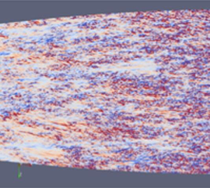
This work considers a prismatic extrusion of the Boeing bump, a Gaussian-shaped bump defined by
 \begin{equation} y(x)=h\exp{\left(-\left(x/x_0 \right)^2 \right)} . \end{equation}
In this equation, the  $x$ coordinate is horizontal and aligned with the freestream flow far upstream of the bump, the $y$ coordinate is normal to the freestream, $h$ is a parameter controlling the bump height and $x_0$ controls the bump length. The curve in (2.1) is exactly the centreline of a three-dimensional (3-D) bump developed at The Boeing Company (Slotnick Reference Slotnick2019) and studied experimentally at the University of Washington (Williams et al. Reference Williams, Samuell, Sarwas, Robbins and Ferrante2020) and the University of Notre Dame (Gray et al. Reference Gray, Gluzman, Thomas, Corke, Lakebrink and Mejia2022). To maintain similarities between the 3-D and two-dimensional (2-D) extruded bumps, the height and length parameters are matched at $h/L=0.085$ and $x_0/L=0.195$, where $L=0.9144\ {\rm m}$ is the length of the square cross-section of the wind tunnel used for the 3-D bump experiments. With these values set, the bump 2-D profile is precisely that employed in DNS in Balin & Jansen (Reference Balin and Jansen2021), Shur et al. (Reference Shur, Spalart, Strelets and Travin2021) and Uzun & Malik (Reference Uzun and Malik2022), although either the Reynolds number or the full domain geometry herein is different from these previous studies.
The set-up of the flow problem and the remainder of the computational domain follow the DNS of Balin & Jansen (Reference Balin and Jansen2021), although updated for the twice larger Reynolds number, and are described by the schematic in figure 1. Based on the freestream velocity of  $U_\infty =32.80\,{\rm m}\,{\rm s}^{-1}$, the flow has a Reynolds number of $Re_L = 2$ million, corresponding to $Re_h=170{\,}000$ when measured against the bump height. In addition, the flow was treated as incompressible due to the small Mach number of $M_\infty =0.09$ (computed using standard sea level conditions). At the location of the inlet to the DNS, shown by the dotted vertical line in figure 1, the momentum thickness Reynolds number is approximately $Re_\theta =1800$, and the boundary layer thickness is roughly $1/9$ of the bump height.

Figure 1. Schematic of the set-up of the flow problem and the remainder of the computational domain following the DNS of Balin & Jansen (Reference Balin and Jansen2021). The solid black curves outline the full domain of the bump flow, whereas the green curves show the boundary layer thickness on both no-slip walls predicted by preliminary RANS. The black dotted lines mark the modified inflow and top boundaries used in the DNS (taken from Balin & Jansen (Reference Balin and Jansen2021) which used the same set-up).
Although the solid curves in figure 1 describe the entire flow domain computed with preliminary RANS, which includes the boundary layer origins on the bottom and top walls at  $x/L=-1.0$, only a fraction of that domain can be feasibly computed by DNS. As outlined in detail in Balin & Jansen (Reference Balin and Jansen2021), the inflow to the DNS domain is moved downstream to $x/L=-0.6$, and the top boundary is slanted downwards according to a profile fitted to the displacement thickness of the Reynolds-averaged Navier–Stokes (RANS) boundary layer on the top wall. The last modification was done to reproduce the constriction effects of the boundary layer growing on the top wall without resolving it. Note that the RANS computations of the full domain were carried out using the Spalart–Allmaras (SA) one-equation model (Spalart & Allmaras Reference Spalart and Allmaras1994) augmented with the rotation and streamline curvature (SARC) correction (Spalart & Shur Reference Spalart and Shur1997; Shur et al. Reference Shur, Strelets, Travin and Spalart2000) and the low-Reynolds-number correction (Spalart & Garbaruk Reference Spalart and Garbaruk2020).
The following boundary conditions were implemented based on the DNS domain shown in figure 1. The bump surface was treated as a no-slip wall. It is worth mentioning that (2.1) defines the entire lower surface of the domain, meaning that there is no flat-plate region on either side of the bump, and the curvature is continuous everywhere. The top surface was modelled as an inviscid wall with zero-velocity component normal to the surface and zero tangential traction. At the outflow, total traction is weakly enforced to zero. In addition, periodic boundary conditions were applied on a spanwise width of  $0.156L$. Finally, at the inflow, the synthetic turbulence generator (STG) of Shur et al. (Reference Shur, Spalart, Strelets and Travin2014) and Patterson, Balin & Jansen (Reference Patterson, Balin and Jansen2021) was utilised to introduce unsteady flow into the domain and rapidly produce mature and realistic turbulence. This STG method was successfully used in the $Re_L = 1$ million DNS of Balin & Jansen (Reference Balin and Jansen2021) and the mean velocity and stress profiles required for the method were obtained following the description therein. Prior to conducting a DNS at $Re_L = 1$ million, our STG method was thoroughly validated on a flat plate in Wright et al. (Reference Wright, Balin, Patterson, Evans and Jansen2020) and Patterson et al. (Reference Patterson, Balin and Jansen2021) where it was determined that the statistics matched those of several published DNS, including ones that computed transition, for $x-x_{inflow} > 5 \delta _{inflow}$. This relatively short development region, combined with an inlet location of $x/L=-0.6$, where the APG is still very weak and thus near our validated flat plate conditions, give us high confidence that our flow has well-developed turbulence for $x/L>-0.56$ which is still significantly upstream of where we later document the boundary layer's physical response first to an APG region that becomes significant around $x/L>-0.5$ and the strong FPG region $-0.3< x/L<0$ that this paper seeks to analyse. In summary, extensive flat plate studies and the previous $Re_L = 1$ million DNS guided the inflow boundary condition's location, type and resolution to ensure that the flow physics produced by this simulation were free of inflow boundary condition artifacts since it would be impractical to run multiple simulations to study boundary conditions at this Reynolds number and geometric complexity.
2.2. Flow solver description
The turbulent boundary layer over the Gaussian bump at  $Re_L = 2$ million discussed herein was computed using a stabilised finite-element method (Whiting & Jansen Reference Whiting and Jansen1999) and second-order accurate, fully implicit generalised- $\alpha$ time integration (Jansen, Whiting & Hulbert Reference Jansen, Whiting and Hulbert2000) to perform time-resolved simulations of the incompressible Navier–Stokes equations. The DNS was carried out using linear mesh elements to reduce the computational cost while still maintaining a high level of accuracy, as demonstrated for a channel flow in Trofimova, Tejada-Martinez & Jansen (Reference Trofimova, Tejada-Martinez and Jansen2009), for a flat plate boundary layer in Wright et al. (Reference Wright, Balin, Patterson, Evans and Jansen2020), and for the Gaussian Bump flow at $Re_L = 1$ million in Balin & Jansen (Reference Balin and Jansen2021). Furthermore, stabilisation and time integration parameters chosen for this DNS follow the work outlined in Trofimova et al. (Reference Trofimova, Tejada-Martinez and Jansen2009) and were similar to those used in Balin & Jansen (Reference Balin and Jansen2021).
The simulations were started from an initial condition with mean velocity and pressure from RANS and superposed fluctuations obtained from DNS at  $Re_L = 1$ million. The initial transient part of the simulation was performed for a half-span domain first, and then the solution was transferred to the full domain using one instantaneous time step for half of the domain and another time step for the other half of the domain. The second time step was chosen such that its reattachment structures were the most out-of-phase from the first to break any domain-width lock in present in the flow. This full domain width initial condition necessarily breaks continuity on the centreline and on the periodic planes but otherwise satisfies the governing equations and the flow solver quickly repaired these breaks. More significant than the time to repair these continuity breaks, the separation point and the reattachment point did show an adjustment to the new domain width and this must be considered part of the transient. Then, after this transient on the full domain, statistics were collected.
While DNS and LES articles often discuss statistics collected in terms of flow through times, this is of less relevance to the bump flow considered for two reasons. First, the flow is not streamwise periodic and also has no global circulation to come to equilibrium and is thus fully determined by the inflow which, via the STG boundary condition, is statistically stationary on a time scale minimised through the choice of random numbers (Patterson et al. Reference Patterson, Balin and Jansen2021). Second, the more relevant time scale to turbulent boundary layers is the eddy turnover time  $\delta (x) / u_e(x)$ which, in this flow varies by a factor of 10 between the most rapid turbulence at the bump peak and the slowest time scale in the thick boundary layer within the recovery region. As this paper is concerned only with the region before separation, the range of eddy turnover times is less dramatic (a factor of 2 between the peak of the weak APG and the bump apex). At the peak of the weak APG, the flow requires about 600 time steps per eddy turnover time. For the plots in this article, we have used statistics windows of at least 32 000 (most used 159 000) time steps which means that this slowest region averages at least 53.33 eddy turnover times. Note further that, to properly model the separated flow region, the domain width is set based on the boundary layer thickness there. In the region of interest to this paper, the boundary layer thickness reaches a local maximum at the peak of the weak APG at a value of 0.015. Thus our domain width is more than 10 local boundary layer thicknesses wide within the domain discussed in this paper. Because we are employing spanwise averaging in our statistics, this means each time step carries roughly 3 times the statistical power of a typical DNS that has a 3 boundary layer thickness domain width. Taken together, this gives at least 160 eddy turnover times in the statistics shown which is well above that of a typical DNS (Spalart Reference Spalart1988). Most of the results shown used 159 000 time steps and thus at least 795 eddy turnover times. This assessment of adequate statistics and sufficient passing of all transients was confirmed by comparing all plots shown on two half-time windows to visually confirm the convergence of statistics.
2.3. Mesh description
Considering the differences in mesh requirements relative to our simulation at  $Re_L = 1$ million (Balin & Jansen Reference Balin and Jansen2021), the mesh for the simulation at $Re_L = 2$ million requires an even higher resolution in the near-wall region and a much larger volume of the domain with turbulent structures due to a much thicker boundary layer downstream of separation. These factors raise the number of grid points required, especially if structured grids are used. To address this challenge, a new unstructured grid mesh generation technique was developed to locally match the grid size to a fixed multiple of the Kolmogorov length scale (e.g. $\varDelta =2\eta$). This approach is regularly carried out for simulations of isotropic turbulence where the isotropic grid size is selected to match the a priori known Kolmogorov length scale that a given forcing and Reynolds number will produce.
However, the situation differs for a complex flow like the bump. Our approach was to make use of prior flat plate boundary layer DNS (Spalart Reference Spalart1988) which established a relationship  $\eta ^+=f(n^+)$ where $n$ is the wall-normal direction making use of predictions of dissipation ( $\epsilon$) profiles in the wall-normal coordinate. This idea is also not completely new as it was applied to pipe and channel flows by Pirozzoli & Orlandi (Reference Pirozzoli and Orlandi2021) independently and concurrently with this effort. The application to boundary layers has a greater opportunity for savings by exploiting the larger growth of $\eta$ in the outer part of the boundary layer. Even larger gains come from the large variation in wall shear stress in this flow, unlike the channels and pipes studied in Pirozzoli & Orlandi (Reference Pirozzoli and Orlandi2021). Here, with this wall-normal variation in dissipation (and thus $\eta$) known, we are able to first set the $\varDelta _n$ spacing for any streamwise location, $s$, so long as an estimate for $u_\tau$ is available for each $s$ location. We make use of RANS simulations to obtain this estimate. While the RANS prediction of $u_\tau$ is known to have some error, it is usually on the high side, which leads to a conservative mesh spacing. The streamwise variation of $u_\tau$ and normal variation of $\eta$ motivate setting mesh sizes not in the Cartesian coordinate system $x$–
$x$– $y$–
$y$– $z$, but rather in one that is locally tangent and normal to the bump surface. This wall-aligned or standard boundary layer coordinate system, hereafter referred to as WCS, has surface varying coordinates $s$–
$s$– $n$–
$n$– $z$, with $s$ being the wall-tangent direction positively aligned with the freestream flow, $n$ being the wall-normal direction always directed into the flow domain (in regions of attached flow $n$ is aligned with the velocity gradient vector at the wall) and $z$ being the spanwise direction obtained by the cross-product of unit vectors along $s$ and $n$. Effectively, this leads to mesh growth curves that emanate from points on the surface and extend in the wall-normal direction $n$ instead of the vertical direction $y$. Note that we also make use of the WCS throughout this paper, including in the analysis of results in § 3.
While the  $n$-point distribution optimisation described above yields significant savings, significantly more savings can be obtained in the streamwise ( $s$) and spanwise ( $z$) spacing. These savings are only available to unstructured grids since a structured grid must satisfy the most strict grid resolution in each direction and propagate that spacing through an $ijk$ grid. Some relief from this constraint is possible for overset grids but this choice faces challenges presented by large jumps in grid size across overset grid interfaces. For this simulation, we have developed and applied mesh generation techniques that smoothly coarsen not only the $n$ direction but also $s$ and $z$. In practice, we employ a wall grid that uses a local streamwise spacing of 15 plus units ( $\varDelta _s^+=u_\tau (s) \varDelta _s(s) /\nu =15$ at the wall) and a local spanwise spacing of 6 plus units ( $\varDelta _z^+=u_\tau (s) \varDelta _z(s) /\nu =6$ at the wall) which was shown to be adequate in Balin & Jansen (Reference Balin and Jansen2021). This requires a triangulated surface mesh to satisfy and realise a growth in spanwise spacing where $u_\tau$ is lower (fewer points in the span). As the first point in the normal direction off of the wall is very small ( $\varDelta ^+_n=u_\tau (s) \varDelta _n(s) /\nu =0.3$ at the wall) to resolve the high gradients there, wedge elements are used to extrude this wall resolution (starting with aspect ratios of $50:1:20$ for $(\varDelta _s:\varDelta _n:\varDelta _z)/\varDelta _n$) normal to the surface. We employ a growth factor of 1.025 until the wall-normal spacing catches up to the desired multiple of $\eta (s)$. At that point, the normal spacing grows with the local Kolmogorov spacing (in this case $2\eta (s,n)$). This is built into the normal spacing described above. Eventually, the growth of the wall-normal spacing catches up to the spanwise spacing. At this point, the extrusion of wedge elements from the surface triangle can be stopped. Subsequent layers then coarsen in the spanwise direction, matching the spanwise spacing to that of normal spacing. This spanwise coarsening can be accomplished with an unstructured grid (and most smoothly accomplished with tetrahedral elements). Therefore, these layers have normal and spanwise spacing matching the desired multiple of Kolmogorov units. The streamwise spacing in these layers is still fixed to what was set by the wall spacing, which continues until the wall-normal (and spanwise) spacing grows larger than the streamwise wall spacing, after which the streamwise spacing also grows. When following this approach, the resulting grid has one-third of the nodes that an equivalent structured grid would have. Reiterating, it accomplishes this by matching a multiple of the local Kolmogorov spacing in all three directions wherever that spacing is larger than the wall plus unit spacing dictated by the local wall shear. As the dissipation and thus Kolmogorov spacing is smooth, so is the gradation of element size in all three directions which is critical to the success of a DNS. Note that while the dissipation function of wall normal variation was taken from prior DNS of flat plates, this choice is conservative for FPGs where the dissipation is reduced and thus $\eta (n)$ grows faster than the flat plate profile assumed. Conversely, in an APG, dissipation is enhanced, making $\eta (n)$ grows slower than the assumed flat plate profile. However, within the weak APG region preceding the strong FPG, $\eta (s,n)$ was confirmed to remain under three which is within DNS requirements for the preseparation regions considered in this paper.
3. Results and analysis
3.1. Boundary layer characterisation
As the experiment's three-dimensionality, even on the centreline, is well documented (Williams et al. Reference Williams, Samuell, Sarwas, Robbins and Ferrante2020; Gray et al. Reference Gray, Gluzman, Thomas, Corke, Lakebrink and Mejia2022), a limited comparison with the DNS of Uzun & Malik (Reference Uzun and Malik2021) is appropriate. However, their DNS had the following differences: (1) location and type of top boundary condition (Riemann boundary condition at  $y=2L$), (2) more narrow domain width ( $L_z=0.08L$), (3) compressible solver and (4) recycling inflow boundary condition. To both compare and understand the differences in the two simulations, we first define the coefficient of pressure ( $C_p$) and skin-friction coefficient ( $C_f$) at the bottom surface as follows,
 \begin{equation} C_p = \frac{\bar{p}_w - p_{\infty}}{\dfrac{1}{2} \rho U_{\infty}^2}, \quad C_f = \frac{\tau_w}{\dfrac{1}{2} \rho U_{\infty}^2}, \end{equation}
where  $\bar {p}_w$ is the pressure at the surface, $p_{\infty }$ is the freestream pressure, $U_{\infty }$ is the freestream speed and $\tau _w$ is the wall shear stress. For $Re_L = 2$ million, we take $U_{\infty } = 32.8\,{\rm m}\,{\rm s}^{-1}$ which is twice the value considered in Balin & Jansen (Reference Balin and Jansen2021). The freestream pressure is chosen so as to match the experimental data by Williams et al. (Reference Williams, Samuell, Sarwas, Robbins and Ferrante2020) at the inflow. We compare $C_p$ and $C_f$ for the two DNSs in figure 2. The results indicate that our DNS predicts a slightly lower $-C_p$ than the other DNS in the mild APG region, $-0.6 \leq x/L \leq -0.29$. In the FPG region, $-0.29 \leq x/L \leq 0$, $-C_p$ is higher for our DNS than the other DNS, especially at the bump peak. These results indicate that the resulting pressure gradient experienced by the boundary layer is different between the two DNSs. In Prakash et al. (Reference Prakash, Balin, Evans and Jansen2022), we showed that these differences are primarily due to the top boundary condition difference, which can be expected (ours is more confined leading to strong pressure gradients) and that these differences in pressure gradients are also the key reason for the differences in $C_f$. The $C_f$ artifact very close to the inflow is due to a very short development period of the STG boundary condition. We obtain a higher $C_f$ than the other DNS until the point of separation. The boundary layer in our DNS separates slightly later and reattaches earlier than the other DNS. The different spanwise lengths also likely influence the location of the boundary layer reattachment point. Similar to the other DNS, a bimodal shape of $C_f$ and $C_p$ in the separated region is observed in our DNS. These results indicate that even though the flow is quantitatively different, the resulting separation flow physics appears to be similar. A more detailed analysis of the differences in simulation set-up and the resulting differences in velocity and stress profiles between the two DNSs are discussed in Appendix A.

Figure 2. Plots of (a)  $C_p$ and (b) $C_f$ for the bump flow at $Re_L = 2$ million. Line types: $\circ$, DNS in Uzun & Malik (Reference Uzun and Malik2022); $\boldsymbol {-}$, Present DNS.
The turbulent boundary layer over the bump experiences varied flow physics. The flow is influenced by changing pressure gradients, from adverse to favourable and back to adverse before flow separation, and varying curvature effects, from concave to convex curvature. In this article, we keep the discussion on pressure gradient and curvature effects limited to the preseparation region of the flow. The effect of pressure gradient on a turbulent boundary layer is commonly quantified using Clauser's pressure gradient parameter (Clauser Reference Clauser1954),
 \begin{equation} \beta = \frac{\delta^*}{\tau_w} \frac{\partial \bar{p}_w}{\partial s}, \end{equation}
where  $\delta ^*$ is the displacement thickness computed based on the integrated vorticity method (Lighthill Reference Lighthill1963; Spalart & Watmuff Reference Spalart and Watmuff1993) and $\partial \bar {p}_w/\partial s$ is the streamwise pressure gradient at the wall. The wall pressure gradient is chosen over the boundary layer edge pressure gradient for several reasons: to avoid sensitivity to the method and threshold (e.g. 99 % or 99.9 %) used to locate the boundary layer edge, to support wall modelling, and to enable better comparison with experiments that usually locate pressure ports on walls. To understand the influence of Reynolds number on these and other parameters, we switch from comparing our results to (Uzun & Malik Reference Uzun and Malik2021) and instead compare with the flow at $Re_L = 1$ million (Balin & Jansen Reference Balin and Jansen2021) which, as noted earlier, matches all boundary conditions except half the inflow speed. The variation of $\beta$ for DNS at $Re_L = 1$ million and $2$ million are shown in figure 3(a) where it is observed that both flows exhibit a relatively mild APG ( $\beta > 0$; maximum $\beta$ is $0.8$ at $x/L \approx -0.35$) and a relatively stronger FPG ( $\beta < 0$; minimum $\beta$ is $-2$ at $x/L \approx -0.17$). Very close to the inflow, the sharp decrease of $\beta$ is attributed to a rise of $C_f$ because of the short development of the inflow boundary condition. The difference in $\beta$ for the $Re_L = 1$ million and $2$ million are small, indicating similar pressure gradient effects for both Reynolds numbers. We compare the boundary layer thickness, $\delta$, computed using the integrated vorticity method specified in Lighthill (Reference Lighthill1963) and Spalart & Watmuff (Reference Spalart and Watmuff1993) with a threshold of 99.9 % for the two $Re_L$ in figure 3(b). Recent work by Griffin, Fu & Moin (Reference Griffin, Fu and Moin2021) provides a simpler and less resolution-sensitive approach to computing the boundary layer thickness which we tested and found to be virtually identical at both 99 % and 99.9 % to the integrated vorticity method, likely because our fine mesh and long statistics resolve well the decay of vorticity. For the two Reynolds number flows, the variation in the boundary layer thickness is similar: an increase in $\delta$ is observed in the mild APG region, and a decrease in $\delta$ is observed in the strong FPG region.

Figure 3. Comparison of (a) Clauser's pressure gradient parameter, (b) boundary layer thickness and (c) Curvature parameter for the bump flow at  $Re_L = 1$ million and $2$ million. Line types: dashed/red, $Re_{L} = 1$ million; full/black, $Re_L = 2$ million.
The effect of curvature on a turbulent boundary layer is quantified using the curvature parameter ( $\delta /{R_w}$), where ${R_w}$ is the radius of curvature of the surface. The direction and sign of ${R_w}$ are defined following the literature on curvature effects. For concave curvature, ${R_w}$ is positive, which implies that the radius of curvature vector, $\boldsymbol {{R_w}}={R_w} \hat {\boldsymbol {n}}$, points from the wall into the flow domain and is positively aligned with $n$. For convex curvature, the opposite is true, thus ${R_w}$ is negative and the curvature vector points from the wall out of the flow domain and opposite to $n$.
$n$.
As shown in figure 3(c), the flow exhibits an initial concave curvature until  $x/L \approx -0.14$ and then switches to convex curvature. The negative peak of $\delta /{R_w}$ is twice as high as the positive peak indicating that the boundary layer experiences more substantial convex curvature effects than the concave curvature effects. This behaviour is because ${R_w}$ is smaller at $x/L = 0$ than its value at $x/L = -0.25$, which offsets the lower value of $\delta$ at $x/L = 0$ compared with its value at $x/L = -0.25$. The flow at $Re_L = 1$ million experiences slightly stronger curvature effects than the flow at $Re_L = 2$ million due to its slightly larger boundary layer thickness for the same geometric curvature.
Although  $\beta$ and $\delta /{R_w}$ variations are qualitatively similar, the turbulent boundary layer exhibits different flow physics for the two Reynolds numbers. These differences are highlighted by comparing friction Reynolds number for the two Reynolds numbers: $Re_{\tau } = u_{\tau } \delta /\nu$, where $u_{\tau } = \sqrt {\tau _w/\rho }$ is the friction velocity. As shown in figure 4, we observe a similar trend for both Reynolds numbers with an increase in $Re_{\tau }$ until $x/L \approx -0.11$. Downstream of that location, $Re_{\tau }$ for $Re_L = 1$ million decreases due to a relaminarising boundary layer. The monotonic increase in $Re_{\tau }$ in the FPG region for $Re_L = 2$ million qualitatively indicates that the pressure gradient effects are not strong enough to trigger relaminarisation and decrease $Re_{\tau }$ within the FPG region. The onset of relaminarisation of a turbulent boundary layer is often quantified based on parameters (Launder Reference Launder1964; Kline et al. Reference Kline, Reynolds, Schraub and Runstadler1967; Patel & Head Reference Patel and Head1968)
 \begin{equation} \varDelta_p = \frac{\nu}{\rho u_{\tau}^3} \frac{\partial \bar{p}}{\partial s}, \quad \text{and} \quad K = \frac{\nu}{\bar{u}_{s,e}^2} \frac{\partial \bar{u}_{s,e}}{\partial s}, \end{equation}
where  $\bar {u}_{s,e}$ is the wall-aligned velocity at the edge of the boundary layer. Several threshold values for these parameters signifying the onset of the relaminarisation process have been proposed over the years (Launder Reference Launder1964; Kline et al. Reference Kline, Reynolds, Schraub and Runstadler1967; Patel & Head Reference Patel and Head1968; Sreenivasan Reference Sreenivasan1982). A commonly used value for indicating relaminarisation is $\varDelta _p = -0.025$ (Patel & Head Reference Patel and Head1968) or $K = 3 \times 10^{-6}$ (Kline et al. Reference Kline, Reynolds, Schraub and Runstadler1967). The variation of $\varDelta _p$ and $K$ for the two Reynolds numbers is shown in figure 5. We observe that the flow for both Reynolds numbers does not cross the relaminarisation threshold. The results for the flow at $Re_L = 1$ million, presented in Balin & Jansen (Reference Balin and Jansen2021) and Uzun & Malik (Reference Uzun and Malik2021), gave evidence of an incomplete relaminarisation process. For $Re_L = 2$ million, the values of $\varDelta _p$ and $K$ are much lower than the common threshold value, and the results for a similar flow (Uzun & Malik Reference Uzun and Malik2022) indicated that the flow does not undergo relaminarisation. As discussed in Sreenivasan (Reference Sreenivasan1982), an accelerated boundary layer exhibits a region of departure from equilibrium scaling laws despite the fully turbulent nature of the flow. This flow region was termed laminarescent (Schraub Reference Schraub1965; Sreenivasan Reference Sreenivasan1982).

Figure 4. Comparison of  $Re_{\tau }$ for the bump flow at $Re_L = 1$ and $2$ million. Line types: dashed/red, $Re_{L} = 1$ million; full/black, $Re_L = 2$ million.

Figure 5. Relaminarisation parameters (a)  $\varDelta _p$ and (b) $K$ for turbulent boundary layer over bump flow at $Re_L = 1$ and $2$ million. Line types: dashed/red, $Re_{L} = 1$ million; full/black, $Re_L = 2$ million.
The onset of laminarescent behaviour of turbulent boundary layers was shown to be at  $\varDelta _p = -0.005$ (Patel Reference Patel1965). This value aligns with the results discussed in Narasimha & Sreenivasan (Reference Narasimha and Sreenivasan1973), where a corrected threshold value of $\varDelta _p = -0.004$ was mentioned. We observe that for $Re_L = 2$ million, this threshold value is crossed $x/L = -0.25$. Evidence of laminarescent behaviour can be observed in the results presented by Uzun & Malik (Reference Uzun and Malik2022) as a significant departure of the streamwise velocity above the logarithmic law and the formation of an inflection point in the Reynolds shear stress in the region $-0.3 \leq x/L \leq -0.2$. The same observations can be made in figure 30 (velocity) and figure 31 (stresses) of Appendix A where we compare and show good agreement of our results with theirs. Therefore, these results indicate that the higher-Reynolds-number flow avoids relaminarisation, as was also observed for the similar flow in Uzun & Malik (Reference Uzun and Malik2022), however the strong FGP effects drive the boundary layer to a laminarescent state. Note that in this laminarescent state, the flow is still fully turbulent. Moreover, Sreenivasan (Reference Sreenivasan1982) further classified this state into two categories: (1) a local flow equilibrium state and (2) a non-equilibrium state. In the local flow equilibrium state, a local similarity analysis could be performed to determine local scaling laws, whereas in the non-local flow equilibrium state, such a local similarity analysis may not be employed.
3.2. SCS analysis
The two-dimensional statistical nature of the flow allows us to consider a local SCS for analysing the flow behaviour. Morse & Mahesh (Reference Morse and Mahesh2021) considered this coordinate system for analysis of the axisymmetric RANS equations to study pressure gradient effects on a submarine hull. Analysis of the momentum budget in the SCS will enable us to isolate the effects of momentum budget terms along and perpendicular to streamlines leading to acceleration along these directions.
We work with a  $\psi$– $\phi$– $z$ SCS, where the $\psi$ direction is locally aligned to be in the direction of the mean velocity vector, the $z$ direction is same as the $z$ direction in the Cartesian and the WCS, and the $\phi$ direction is orthogonal to the $\psi$ and $z$ directions based on the right-hand rule (i.e. positively aligned with $n$ for the attached portion of the flow considered here). Representing relevant statistics in this coordinate system allows us to understand the flow behaviour in directions parallel and perpendicular to the streamlines. The attached boundary layers considered herein cause small, locally varying turning of the streamline towards and away from the wall. This behaviour leads to the evolution of the SCS locally in space in contrast to the WCS mentioned in Bradshaw (Reference Bradshaw1973), which does not vary in the wall-normal direction. From here on, the subscript indicates the direction of the vector component; for example, $\bar {u}_{\psi }$ is the component of averaged velocity in the $\psi$ direction. As the word normal refers both to direction and to diagonal components of stresses, we use the unambiguous math definition of the normal Reynolds stresses instead of words (e.g. $\overline {u'_\psi u'_\psi }$ instead of the first normal stress in the SCS). If we were to represent the continuity and momentum equations in the SCS, a simple rotation of terms would not suffice as the local coordinate system also changes in space. Therefore, the derivation of continuity and momentum equations in the SCS involves principles from differential geometry. This problem was chased in Finnigan (Reference Finnigan1983), and the physical interpretation of different terms was discussed. As the streamline normal velocity ( $\bar {u}_{\phi }$) is zero in the SCS, the mean continuity equation is trivially satisfied in the SCS for incompressible flows (Finnigan Reference Finnigan1983). In the absence of gravity forces, the steady mean momentum equations in the streamline coordinate system (Finnigan Reference Finnigan1983) are given as follows:
 \begin{align} \bar{u}_{\psi} \frac{\partial \bar{u}_{\psi}}{\partial \psi} &=-\frac{1}{\rho} \frac{\partial \bar{p}}{\partial \psi} - \frac{\partial \overline{u'_{\psi} u'_{\psi}}}{\partial \psi} - \frac{\partial \overline{u'_{\psi} u'_{\phi}}}{\partial \phi} + \frac{\overline{u'_{\psi} u'_{\psi}} - \overline{u'_{\phi} u'_{\phi}}}{L_a} + 2\frac{\overline{u'_{\psi} u'_{\phi}}}{{R_\psi}}\nonumber\\ &\quad + \nu \left[ \frac{\partial^2 \bar{u}_{\psi}}{\partial \psi^2} + \frac{\partial^2 \bar{u}_{\psi}}{\partial \phi^2} - \frac{2}{L_a} \frac{\partial \bar{u}_{\psi}}{\partial \psi} - \frac{1}{{R_\psi}} \frac{\partial \bar{u}_{\psi}}{\partial \phi} - \frac{\bar{u}_{\psi}}{{R_\psi^2}} \right], \end{align}
 \begin{align} \frac{\bar{u}_{\psi}^2}{{R_\psi}} &=-\frac{1}{\rho} \frac{\partial \bar{p}}{\partial \phi} - \frac{\partial \overline{u'_{\phi} u'_{\psi}}}{\partial \psi} - \frac{\partial \overline{u'_{\phi} u'_{\phi}}}{\partial \phi} + 2\frac{\overline{u'_{\psi} u'_{\phi}}}{L_a} + \frac{ \overline{u'_{\psi}u'_{\psi}} - \overline{u'_{\phi} u'_{\phi}}}{{R_\psi}}\nonumber\\ &\quad + \nu \left[ - \frac{\partial^2 \bar{u}_{\psi}}{\partial \psi \partial \phi} + \frac{1}{L_a} \frac{\partial \bar{u}}{\partial \phi} + \frac{\partial }{\partial \psi} \left( \frac{\bar{u}_{\psi}}{{R_\psi}} \right) + \frac{\bar{u}_{\psi}}{{R_\psi} L_a} \right], \end{align}
where  $L_a$ is known as the ‘e-folding’ distance that characterises the length scale for streamwise acceleration and ${R_\psi }$ is the local radius of curvature of the streamline. These two quantities can be computed as follows:
 \begin{equation} \frac{\bar{u}_{\psi}}{L_a} = \frac{\partial \bar{u}_{\psi}}{\partial \psi}, \quad \frac{1}{{R_\psi}} = \frac{1}{\bar{u}_{\psi}} \left( \varOmega + \frac{\partial \bar{u}_{\psi}}{\partial \phi} \right), \end{equation}
where  $\varOmega$ is the magnitude of mean vorticity based on the right-hand coordinate system. In our simulation, we collect statistics (average in time and spanwise direction) for the velocity, velocity products, pressure, and pressure squared in the Cartesian coordinate system. From the averaged velocity vector, the streamline direction can be determined at each point and all statistics can be rotated pointwise into the SCS at every $x,y$ point on the periodic plane of the DNS mesh. As that mesh is fine enough to resolve the instantaneous turbulence structures, we are able to compute the fields (including Reynolds stresses) and their gradients very accurately to obtain the quantities shown in (3.4) and (3.5) and other analyses within this paper. In (3.4), the first term on the right-hand side can be combined with the term on the left-hand side resulting in a total pressure gradient term. With this change, the equation indicates that the total pressure is conserved along the streamlines when the viscous and turbulent momentum fluxes are negligible, which aligns with Bernoulli's principle. In the next section, we present non-dimensional budgets of the momentum equations where inner units, $u_{\tau }^3/\nu$, are used to normalise the budget terms on the ordinate. These are plotted vs non-dimensional wall distances normalised by $\nu /u_{\tau }$ and $\delta$ for presenting the results in inner and outer regions of the boundary layer, respectively.
3.2.1.  $\varPsi$-momentum budget in the SCS

Assessing the momentum equation budget in the SCS allows us to characterise the dominant forces acting on a fluid packet following the streamlines. In figure 6(a), we show the  $\varPsi$-momentum budget in the near-wall region at $x/L = -0.35$, the location of the maximum APG. We observe that the momentum transfer due to the turbulent and viscous fluxes (defined in the second line of (3.4)) is the most dominant. The small difference between the two momentum fluxes is balanced by the pressure gradient close to the wall. The advection term is much smaller than the pressure gradient near the wall. The $\varPsi$-momentum budget far from the wall is shown in figure 6(b). We observe that momentum fluxes due to viscous effects are negligible in this region. The momentum flux due to the Reynolds shear stress term is almost balanced by the total pressure gradient term (advection + pressure gradient), and the slight differences which are not visible on this scale are attributed to the momentum flux due to $\overline {u'_\psi u'_\psi }$. A net negative value of advection momentum transfer is observed, indicating deceleration of the streamlines in the mild APG region. The budget behaviour in both the inner and outer regions of the boundary layer is similar at other locations in the APG region.

Figure 6. The  $\varPsi$-momentum budget stations at $x/L = -0.35$ in APG region. The $x$-axis is normalised in (a) inner units and (b) outer units, whereas the $y$-axis is normalised in inner units. Line types: blue, $\bar {u}_{\psi } \,{\rm d} \bar {u}_{\psi }/{\rm d}\psi$; black, ${\rm d}\bar {p}/{\rm d}\psi$; green, ${\rm d}\overline {u'_{\psi } u'_{\psi }}/{\rm d}\psi$; orange, ${\rm d}\overline {u'_{\psi } u'_{\phi }}/{\rm d}\phi$; red, $- (\overline {u'_{\psi }u'_{\psi }} - \overline {u'_{\phi }u'_{\phi }})/L_a$; cyan, $-2\overline {u'_{\psi } u'_{\phi }}/{R_\psi }$; magenta, negative of viscous terms; yellow, budget balance. Note that the difference in $y$-axis limits for (a,b) highlight the difference in magnitude of these terms in the inner and outer regions of the flow.
In figure 7, we show the  $\varPsi$-momentum budget in the near-wall region for three different $x/L$ locations corresponding to the start of the FPG region, close to the location of the maximum FPG and near the end of the FPG region. We observe that the momentum fluxes due to viscous forces, turbulence and pressure gradient balance very close to the wall. The advection term grows significantly after $n^+ > 10$ and this increase appears to have a log-linear dependence on $n^+$. The behaviour in the outer region of the boundary layer is shown in figure 8. The outer region of the boundary layer is dominated by momentum flux due to the pressure gradient, advection and turbulence terms. In this region, there is a positive value of the advection momentum flux, which indicates a net acceleration of the streamlines in the FPG region. Like the APG region, the pressure gradient, advection and Reynolds shear stress terms are mostly balanced with the next largest term (not quite visible on this scale) being the $\overline {u'_\psi u'_\psi }$ term. From these results, we observe that the dominant terms of the momentum equation budget in both the APG and FPG regions are: viscous flux, turbulence shear flux, pressure gradient and advection flux.

Figure 7. The  $\varPsi$-momentum budget at several $x/L$ stations in the FPG region: (a) $x/L = -0.29$; (b) $x/L = -0.15$; (c) $x/L = -0.05$. Both axes are normalised by inner units. Line types: blue, $\bar {u}_{\psi } \,{\rm d} \bar {u}_{\psi }/{\rm d}\psi$; black, ${\rm d}\bar {p}/{\rm d}\psi$; green, ${\rm d}\overline {u'_{\psi } u'_{\psi }}/{\rm d}\psi$; orange, ${\rm d}\overline {u'_{\psi } u'_{\phi }}/{\rm d}\phi$; red, $- (\overline {u'_{\psi } u'_{\psi }} - \overline { u'_{\phi } u'_{\phi }})/L_a$; cyan, $-2\overline {u'_{\psi } u'_{\phi }}/{R_\psi }$; magenta, negative of viscous terms; yellow, budget balance.

Figure 8. The  $\varPsi$-momentum budget at several stations in the FPG region: (a) $x/L = -0.29$; (b) $x/L =-0.15$; (c) $x/L = -0.05$. The $x$-axis is normalised in outer units, whereas the $y$-axis is normalised in inner units. Line types: blue, $\bar {u}_{\psi } \,{\rm d} \bar {u}_{\psi }/{\rm d}\psi$; black, ${\rm d}\bar {p}/{\rm d}\psi$; green, ${\rm d}\overline {u'_{\psi } u'_{\psi }}/{\rm d}\psi$; orange, ${\rm d}\overline {u'_{\psi } u'_{\phi }}/{\rm d}\phi$; red, $- (\overline {u'_{\psi } u'_{\psi }} - \overline {u'_{\phi } u'_{\phi }})/L_a$; cyan, $-2\overline {u'_{\psi } u'_{\phi }}/{R_\psi }$; magenta, negative of viscous terms; yellow, budget balance.
3.2.2. $\varPhi$-momentum budget in the SCS

The  $\varPhi$-momentum budget enables the assessment of forces normal to the streamlines acting on a fluid packet moving along the streamlines. In figure 9(a), we show the $\varPhi$-momentum budget in the near-wall region for the APG region of the flow. At $x/L = -0.35$, we observe fluxes due to $\overline {u'_\phi u'_\phi }$ term and pressure gradient balance each other until $n^+ \approx 10$. The effects of curvature are observed from $n^+ \geq 10$ onwards in figure 9(a,b). We observe that the difference between the momentum flux due to the pressure gradient and $\overline {u'_\phi u'_\phi }$ term is non-zero. The net difference is equal to the advection normal to the streamlines.

Figure 9. The  $\varPhi$-momentum budget at $x/L = -0.35$ in the APG region. The $x$-axis is normalised in (a) inner units and (b) outer units, whereas the $y$-axis is normalised in inner units. Line types: black, $\bar {u}_{\psi }^2/{R_\psi }$; blue, ${\rm d}\bar {p}/{\rm d}\phi$; green, ${\rm d} \overline {u'_{\psi } u'_{\phi }}/{\rm d} \psi$; orange, ${\rm d}\overline {u'_{\phi } u'_{\phi }}/{\rm d} \phi$; red, $-2\overline {u'_{\psi } u'_{\phi }}/L_a$; cyan, $-(\overline {u'_{\psi } u'_{\psi }} - \overline {u'_{\phi } u'_{\phi })}/{R_\psi }$; magenta, negative of viscous terms; yellow, budget balance.
In figures 10 and 11, we show the  $\varPhi$-momentum budget at three different $x/L$ locations in the FPG region of the flow. We observe that the FPG region shows similar behaviour as the APG region until $x/L = -0.14$. For $-0.14 \leq x/L \leq 0$, the difference between momentum fluxes due to $\overline {u'_\phi u'_\phi }$ and pressure gradient results in a net acceleration of streamlines. This behaviour reduces the momentum in the outer region of the boundary layer and brings it into the inner region of the boundary layer leading to the decay of turbulence in the outer region of the boundary layer. From the $\varPhi$-momentum budget, we observe that the pressure gradient normal to the streamlines and the $\overline {u'_\phi u'_\phi }$ term are the dominant components for the momentum budget that governs the acceleration of streamlines towards or away from the wall.

Figure 10. The  $\varPhi$-momentum budget at several $x/L$ stations in FPG region: (a) $x/L = -0.29$; (b) $x/L = -0.15$; (c) $x/L = -0.05$. Both axes are normalised by inner units. Line types: black, $\bar {u}_{\psi }^2/{R_\psi }$; blue, ${\rm d}\bar {p}/{\rm d}\phi$; green, ${\rm d} \overline {u'_{\psi } u'_{\phi }}/{\rm d} \psi$; orange, ${\rm d}\overline {u'_{\phi } u'_{\phi }}/{\rm d} \phi$; red, $-2\overline {u'_{\psi } u'_{\phi }}/L_a$; cyan, $-(\overline {u'_{\psi } u'_{\psi }} - \overline { u'_{\phi } u'_{\phi }})/{R_\psi }$; magenta, negative of viscous terms; yellow, budget balance.

Figure 11. The  $\varPhi$-momentum budget at several $x/L$ stations in FPG region: (a) $x/L = -0.29$; (b) $x/L = -0.15$; (c) $x/L = -0.05$. The $y$-axis is normalised by inner units whereas the $x$-axis is normalised by outer units. Line types: black, $\bar {u}_{\psi }^2/{R_\psi }$; blue, ${\rm d}\bar {p}/{\rm d}\phi$; lime, ${\rm d} \overline {u'_{\psi } u'_{\phi }}/{\rm d} \psi$; orange, ${\rm d}\overline {u'_{\phi } u'_{\phi }}/{\rm d} \phi$; red, $-2\overline {u'_{\psi }u'_{\phi }}/L_a$; cyan, $-(\overline {u'_{\psi } u'_{\psi }} - \overline {u'_{\phi } u'_{\phi }})/{R_\psi }$; magenta, negative of viscous terms; yellow, budget balance.
3.3. Integral analysis-based Reynolds stress approximations
Simplified momentum equations were integrated normal to the wall in Knopp et al. (Reference Knopp, Buchmann, Schanz, Eisfeld, Cierpka, Hain, Schröder and Kähler2015) and Romero et al. (Reference Romero, Zimmerman, Philip and Klewicki2022) to determine an approximation for a component of the Reynolds shear stress. They proposed using this approximate stress as a normalisation for turbulent statistics in the inner region units of turbulent boundary layers. In this section, we extend this analysis to consider the physics exhibited by the bump flow where the advection and centrifugal acceleration terms become prominent. Further, this analysis is also extended to the outer region of the turbulent boundary layer. We acknowledge that, since this approach arrives at this Reynolds stress approximation through an integration of the momentum equation normal to the wall, some may find referring to it as a scale or scaling misleading. Here, we do not claim that this term is a scale in the fundamental sense that the word scale is used in the turbulence literature but we instead refer to these terms as an approximation used for normalising Reynolds stresses rather than a scale or scaling of Reynolds stress profiles.
3.3.1. Inner region
We draw insights from the  $\varPsi$-momentum budget to obtain a non-local approximation for the Reynolds shear stress. From the $\varPsi$-momentum budgets shown in § 3.2.1, we observe that only a few terms contribute to the momentum fluxes: viscous stress, Reynolds shear stress and pressure gradient, thereby leading to a net acceleration or inertia along the streamlines. Therefore, the $\varPsi$-momentum budget (3.4) reduces to
 \begin{equation} \bar{u}_{\psi} \frac{\partial \bar{u}_{\psi}}{\partial \psi} \approx-\frac{1}{\rho} \frac{\partial \bar{p}}{\partial \psi} - \frac{\partial \overline{u'_{\psi} u'_{\phi}}}{\partial \phi} + \nu \frac{\partial^2 \bar{u}_{\psi}}{\partial \phi^2}. \end{equation}
Rearranging the equation and integrating the equation along  $\phi$ holding $\psi$ fixed results in
 \begin{equation} -\overline{u'_{\psi} u'_{\phi}} + \nu \frac{\partial \bar{u}_{\psi}}{\partial \phi} \approx \int_{0}^{\phi} \left( \bar{u}_{\psi} \frac{\partial \bar{u}_{\psi}}{\partial \psi} + \frac{1}{\rho} \frac{\partial \bar{p}}{\partial \psi} \right) \,{\rm d} \phi' + \frac{\tau_w}{\rho}. \end{equation}
Sufficiently far away from the wall, the viscous term is negligible, and the equation simplifies to
 \begin{equation} -\overline{u'_{\psi} u'_{\phi}} (\phi) \approx \int_{0}^{\phi} \left( \bar{u}_{\psi} \frac{\partial \bar{u}_{\psi}}{\partial \psi} + \frac{1}{\rho} \frac{\partial \bar{p}}{\partial \psi} \right) \,{\rm d} \phi' + \frac{\tau_w}{\rho}. \end{equation}
Integrating along  $\phi$ is quite challenging and far more complicated than $n$ lines.
To understand the potential error incurred by integrating along  $n$ lines, in figure 12, we plot the angle between the streamlines and the wall, $\varDelta _{\theta }$. In the mild APG region, the streamlines within the boundary layer deviate away from the wall. The first profile at $x/L=-0.5$ shows a boundary layer edge streamline angle of $0.007$ rad. As the APG increases $\varDelta _\theta$ grows but then, as the pressure gradient relaxes to zero just past the APG–FPG switch, the streamlines become nearly parallel to the surface in the boundary layer. In the FPG region, the streamlines deflect toward the wall. We observe that in both the APG and FPG regions, the streamlines deviate from the surface by less than $0.005$ rad ( $0.3^{\circ }$) below $y^+=100$ and less than $0.05$ rad ( $3^{\circ }$) throughout. Thus, in the integral analysis that follows, the SCS integrands will be sampled and integrated along $n$ lines to obtain approximations. The small difference in the $n$ and $\phi$ direction means the SCS and the WCS are nearly aligned which will also allow us to apply the analysis in both the SCS and the WCS which is important since the WCS is where simulations and modelling are more practical.

Figure 12. The angle of deflection (in radians) of streamlines from the bump surface in (a) APG region and (b) FPG region. Here  $\star$ indicates the edge of the boundary layer. Line types for APG region at $x/L$: violet, $-0.5$; cerulean, $-0.45$; green, $-0.39$; orange, $-0.35$; mahogany, $-0.3$. Line types for FPG region at $x/L$: violet, $-0.29$; royal blue, $-0.25$; cyan, $-0.2$; sea green, $-0.15$; green, $-0.1$; yellow orange, $-0.079$; red orange, $-0.05$; mahogany, $-0.006$.
In the inner region of the boundary layer the close alignment of the SCS with WCS allows (3.9) to be approximated by
 \begin{equation} -\overline{u'_{\psi} u'_{\phi}} (n) \approx \int_{0}^{n} \left( \bar{u}_{\psi} \frac{\partial \bar{u}_{\psi}}{\partial \psi} + \frac{1}{\rho} \frac{\partial \bar{p}}{\partial \psi} \right) \,{\rm d} n' + \frac{\tau_w}{\rho}, \end{equation}
where in this approximation the integral is taken along a curve where  $s$ is fixed (a straight line ray normal from the wall at a given point on the surface corresponding to $s$).
$s$).
The first term on the right-hand side of the above equation accounts for the effect of streamline acceleration, and the second term on the right-hand side accounts for pressure gradient effects. We can define an approximation,
 \begin{equation} u^2_{*,i} (n) \stackrel{\text{def}}= \int_{0}^{n} \left( \bar{u}_{\psi} \frac{\partial \bar{u}_{\psi}}{\partial \psi} + \frac{1}{\rho} \frac{\partial \bar{p}}{\partial \psi} \right) \,{\rm d} n' + \frac{\tau_w}{\rho}, \end{equation}
which could normalise the Reynolds shear stress in the SCS as
 \begin{equation} \frac{-\overline{u'_{\psi} u'_{\phi}}}{u_{*,i}^2} \approx 1. \end{equation}
The above equation indicates that the normalised shear stress in the SCS is independent of Reynolds number, pressure gradient and acceleration effects. By assuming that the misalignment of SCS and WCS is sufficiently small, we can extend this analysis to the Reynolds shear stress in the WCS.
 \begin{equation} \frac{-\overline{u'_{s} u'_{n}}}{u_{*,i}^2} \approx 1. \end{equation}
If the acceleration and pressure gradient terms are negligible,  $u^2_{*,i} \approx u^2_{\tau }$, indicating that the Reynolds shear stress in the WCS normalises independently of the Reynolds number and follows the classical Reynolds shear stress normalisation used for zero pressure gradient turbulent boundary layers. When the acceleration term is negligible but pressure gradient effects are still significant in the inner region of the boundary layer, the approximation reduces to
 \begin{equation} u^2_{*,i} (n) \approx \int_{0}^{n} \frac{1}{\rho} \frac{\partial \bar{p}}{\partial \psi} \,{\rm d} n' + \frac{\tau_w}{\rho} . \end{equation}
Assuming that the pressure gradient is constant in the wall-normal direction, we attain the following:
 \begin{equation} u^2_{*,i} (n) \approx \frac{n}{\rho} \frac{\partial \bar{p}}{\partial \psi} + u_{\tau}^2 , \end{equation}
which is similar to the hybrid velocity normalisation presented in Sekimoto et al. (Reference Sekimoto, Kitsios, Atkinson and Soria2019) and Romero et al. (Reference Romero, Zimmerman, Philip and Klewicki2022). This observation indicates that, subject to appropriate assumptions of negligible advection or pressure gradient effects, the derived approximation reduces to other commonly used normalisations for the Reynolds shear stress (e.g.  $u_\tau$ when both absent).
We compare the Reynolds shear stress profiles in the APG region with different normalisations in figure 13. We observe that the friction velocity normalisation does not collapse at all  $x/L$ stations. At $x/L = -0.5$ and $-0.45$, the pressure gradient is slight, and the Reynolds shear stress profiles collapse and agree well with theoretical estimates of $-\overline {u'_{s} u'_{n}}/u_{\tau }^2 \approx 1$ sufficiently far away from the wall in the inner region of the boundary layer. As the APG increases for later downstream locations, and as $u^2_{\tau }$ does not fully account for it, the results deviate from theoretical estimates and the curves do not collapse. On the other hand, the use of $u^2_{*,i}$ for normalisation accounts for the effect of pressure gradients and the resulting acceleration, thereby collapsing the velocity profiles to the theoretical values $-\overline {u'_{s} u'_{n}}/u_{*,i}^2 \approx 1$ in the inner region of the boundary layer. This analysis indicates that the normalised Reynolds shear stress in the inner region of the boundary layer depends on streamwise acceleration, streamwise pressure gradient and wall shear stress. Unfortunately, $u^2_{*,i}$ decreases faster than the rate for $-\overline {u'_{s} u'_{n}}$ in the outer region of the boundary layer, forming a singularity that makes the normalisation ineffective far away from the wall. Furthermore, we also tested the approximation in (3.15) and observed that it gives a good collapse of stress profiles in the inner region in the early parts of the mild APG region. However, it fails to collapse the stress profile at $x/L \approx -0.3$. This observation indicates that accounting for all significant terms is essential to the success of the normalisation.

Figure 13. Reynolds shear stress in WCS in the APG region using (a)  $u^2_{\tau }$ and (b) $u^2_{*,i}$. Vertical lines indicate that the quantity asymptotically goes to $\pm \infty$. Line types for APG region at $x/L$: violet, $-0.5$; cerulean, $-0.45$; green, $-0.39$; orange, $-0.35$; mahogany, $-0.3$.
When extracting physical insight from simulations, it is important to be certain that the results are not significantly influenced by boundary conditions. In particular, the collapse of the stress profiles when using  $u^2_{*,i}$ throughout the APG region shown in figure 13, including at $x/L=-0.5$, greatly bolsters confidence in our assertion that the STG boundary condition is not introducing artifacts into this simulation since it seems highly unlikely for those artifacts to also lead to this collapse. Rather, we maintain that the flow has matured quickly into correct turbulence under the weak APG at the inflow which then allows the simulation to accurately reflect the physics of the smoothly increasing and then smoothly decreasing APG. Further, as the FPG region is even further downstream, we are confident it is also free of STG inflow artifacts.
We compare the Reynolds shear stress profiles in the WCS in the FPG region with different normalisations in figure 14. We observe that for all  $x/L$ stations in the FPG, the friction velocity normalisation does not collapse the shear stress profiles in the inner region of the boundary layer. On the other hand, the new Reynolds shear stress approximation leads to a much better collapse of the Reynolds shear stress profiles in the inner region. Note that the flow is experiencing pressure gradients leading to acceleration, the presence of an internal layer, and concave and convex curvature effects in this region. Even with such complex flow physics, the Reynolds shear stress profiles collapse well. Even though the collapse is good, we expected it to be better in the buffer region $n^+ < 30$. While deriving the approximation, we assumed that the viscous effects are negligible sufficiently far from the wall. This assumption may not hold in the FPG region where the strong pressure gradient effects lead to the laminarescent stage, where the boundary layer adjusts towards starting the relaminarisation process. Therefore, we would expect viscous effects to be important even further away from the wall, and these effects should also be incorporated into the approximation. From (3.8) and assuming the misalignment between the SCS and WCS is sufficiently small, we attain
 \begin{equation} -\overline{u'_{\psi} u'_{\phi}} (n) \approx \int_{0}^{n} \left( \bar{u}_{\psi} \frac{\partial \bar{u}_{\psi}}{\partial \psi} + \frac{1}{\rho} \frac{\partial \bar{p}}{\partial \psi} \right) \,{\rm d} n' + \frac{\tau_w}{\rho} - \nu \frac{\partial \bar{u}_{\psi}}{\partial \phi}, \end{equation}
leading to a new approximation,  $u^2_{**,i}$,
 \begin{equation} \frac{ -\overline{u'_{s} u'_{n}}}{u^2_{**,i}} \approx 1, \quad \text{where} \ u^2_{**,i} (n) \stackrel{\text{def}}= \int_{0}^{n} \left( \bar{u}_{\psi} \frac{\partial \bar{u}_{\psi}}{\partial \psi} + \frac{1}{\rho} \frac{\partial \bar{p}}{\partial \psi} \right) \,{\rm d} n' + \frac{\tau_w}{\rho} - \nu \frac{\partial \bar{u}_{\psi}}{\partial \phi} . \end{equation}
Figure 14. Reynolds shear stress in WCS in the FPG region normalised by (a)  $u^2_{\tau }$ and (b) $u^2_{*,i}$. Vertical lines indicate that the quantity asymptotically goes to $\pm \infty$. Line types for FPG region at $x/L$: violet, $-0.29$; royal blue, $-0.25$; cyan, $-0.2$; sea green, $-0.15$; green, $-0.1$; yellow orange, $-0.079$; red orange, $-0.05$; mahogany, $-0.006$.
We show the Reynolds shear stress normalised using  $u^2_{**,i}$ in figure 15. The $u^2_{**,i}$ normalisation does not significantly affect the already good collapse of stress profiles in the APG region compared with $u^2_{*,i}$. However, it substantially improves the collapse of Reynolds shear stress profiles in the FPG region in both the buffer and log regions ( $10 \leq n^+ \leq 100$) of the boundary layer compared with $u^2_{*,i}$ normalisation. These results indicate that for flows where viscous effects become substantial, the normalisation of the Reynolds shear stress must be adjusted to account for the thick near-wall viscous region. Furthermore, with a better collapse of Reynolds shear stress profiles with this proposed approximation, it appears that the upstream history effects and development of internal layers are also accounted for.

Figure 15. Reynolds shear stress in WCS in the (a) APG region and (b) FPG region normalised by  $u^2_{**,i}$. Vertical lines indicate that the quantity asymptotically goes to $\pm \infty$. Line types for APG region at $x/L$: violet, $-0.5$; cerulean, $-0.45$; green, $-0.39$; orange, $-0.35$; mahogany, $-0.3$. Line types for FPG region at $x/L$: violet, $-0.29$; royal blue, $-0.25$; cyan, $-0.2$; sea green, $-0.15$; green, $-0.1$; yellow orange, $-0.079$; red orange, $-0.05$; mahogany, $-0.006$.
Even though these new approximations show good collapse of the Reynolds shear stress, they should not be expected to and do not show good collapse for Reynolds normal stresses. Therefore, we derive the approximation for  $\overline {u'_n u'_n}$ stress by a similar procedure. In this case, we consider the $\varPhi$-momentum budget, (3.5) and remove all the equation components that had negligible influence as observed in § 3.2.1,
 \begin{equation} \frac{\bar{u}_{\psi}^2}{{R_\psi}} \approx-\frac{1}{\rho} \frac{\partial \bar{p}}{\partial \phi} - \frac{\partial \overline{u'_{\phi} u'_{\phi}}}{\partial \phi}. \end{equation}
Rearranging this equation and integrating it along  $\phi$, we obtain
 \begin{equation} \overline{u'_{\phi} u'_{\phi}} (\phi) \approx- \int_{0}^{\phi} \left( \frac{\bar{u}_{\psi}^2}{{R_\psi}} + \frac{1}{\rho} \frac{\partial \bar{p}}{\partial \phi} \right) \,{\rm d} \phi' \approx- \int_{0}^{\phi} \frac{\bar{u}_{\psi}^2}{{R_\psi}} \,{\rm d} \phi' + \frac{\bar{p}_w - p}{\rho}. \end{equation}
To simplify the calculation, we again assume near-alignment of the SCS and WCS and using  ${R_w}$ in place of ${R_\psi }$, which are both valid as shown in figure 12
 \begin{equation} \overline{u'_{\phi} u'_{\phi}} (n) \approx- \int_{0}^{n} \frac{\bar{u}_{\psi}^2}{{R_w}} \,{\rm d} n' + \frac{\bar{p}_w - p}{\rho}. \end{equation}
Therefore, we can define a new approximation for  $\overline {u'_\phi u'_\phi }$
 \begin{equation} u^2_{\gamma,i} (n) \stackrel{\text{def}}=- \int_{0}^{n} \frac{\bar{u}_{\psi}^2}{{R_w}} \,{\rm d} n' + \frac{\bar{p}_w - p}{\rho}, \end{equation}
which satisfies the following equation in the near-wall region:
 \begin{equation} \frac{ \overline{u'_{\phi} u'_{\phi}}}{u^2_{\gamma,i}} \approx \frac{ \overline{u'_{n}u'_{n}}}{u^2_{\gamma,i}} \approx 1, \end{equation}
which gives a normalisation for  $\overline {u'_n u'_n}$. The expression for $u^2_{\gamma,i}$ indicates that $\overline {u'_n u'_n}$ dynamically depends on the centrifugal force and local pressure. In the absence of the streamline curvature effects, the centrifugal force term is expected to be negligible, resulting in a dependence on the difference between the local pressure and the pressure at the wall.
The normalised  $\overline {u'_n u'_n}$ stress for the APG and FPG regions are shown in figures 16 and 17, respectively. We observe that the $u^2_{\tau }$ normalisation does not lead to a collapse of stress profiles in both the APG and FPG regions. Using $u^2_{\gamma,i}$ for normalising the stress profile, we get a much better collapse and agreement with the theoretical estimates in the inner boundary layer region for both the APG and FPG regions of the flow. These results indicate that including the local pressure gradient and centrifugal force terms is important to account for the dynamics of these quantities in the normalisation. Our analysis leads to the derivation of approximations for $\overline {u'_{s} u'_{n}}$ and $\overline { u'_{n} u'_{n}}$. However, these derived approximations are specific to $\overline { u'_{s} u'_{n}}$ and $\overline {u'_{n} u'_{n}}$, and do not extend well to other Reynolds stress components: $\overline {u'_{s} u'_{s}}$ and $\overline {u'_z u'_z}$.

Figure 16. Plots of  $\overline {u'_n u'_n}$ in APG region normalised by (a) $u^2_{\tau }$ and (b) $u^2_{\gamma,i}$. Vertical lines indicate that the quantity asymptotically goes to $\pm \infty$. Line types for APG region at $x/L$: violet, $-0.5$; cerulean, $-0.45$; green, $-0.39$; orange, $-0.35$; mahogany, $-0.3$.

Figure 17. Plots of  $\overline {u'_n u'_n}$ in FPG region normalised by (a) $u^2_{\tau }$ and (b) $u^2_{\gamma,i}$. Vertical lines indicate that the quantity asymptotically goes to $\pm \infty$. Line types for FPG region at $x/L$: violet, $-0.29$; royal blue, $-0.25$; cyan, $-0.2$; sea green, $-0.15$; green, $-0.1$; yellow orange, $-0.079$; red orange, $-0.05$; mahogany, $-0.006$.
3.3.2. Outer region
Before deriving the approximations for the Reynolds stresses in the outer region using integral analysis, we first define some commonly used normalisations. The normalisation of the Reynolds stresses in the outer region is often represented using the defect law for the Reynolds stress tensor (Clauser Reference Clauser1956; Castillo & George Reference Castillo and George2001):
 \begin{equation} \frac{\overline{u'_i u'_j}}{R_{ij,o}} = f_{ij} \left(\frac{n}{\delta}\right), \end{equation}
where  $R_{ij,o}$ is the normalisation for $ij$th component of the Reynolds stress tensor in the outer region of the boundary layer. If the normalisation for Reynolds stresses is based on the same velocity normalisation in both the inner and outer region of the boundary layer (Clauser Reference Clauser1954), then the friction velocity is used for normalising the stresses in the outer region and $R_{ij,o} = u_{\tau }^2$. Similarly, two velocity normalisation approaches can be taken for the Reynolds stresses, where $R_{ij,i} = u_{\tau }^2 \ne R_{ij,o}$. Using similarity analysis, Castillo & George (Reference Castillo and George2001) derived a normalisation for the Reynolds stresses in the outer region of the turbulent boundary layer in the WCS as
 \begin{equation} R_{sn,o} = \bar{u}_s^2 \frac{\partial \delta}{\partial s}, \quad R_{ss,o} = \bar{u}_s^2, \quad R_{nn,o} = \bar{u}_s^2. \end{equation}
Brzek et al. (Reference Brzek, Turan, Anderson and Castillo2005) showed that this normalisation does not collapse the stress profiles in the presence of pressure gradients. Another common outer region velocity normalisation is Zagarola–Smits normalisation,
 \begin{equation} U_{ZS} = \bar{u}_{s,e}\frac{\delta^*}{\delta}, \end{equation}
where  $\bar {u}_{s,e}$ is the velocity at the edge of boundary layer and $\delta ^*$ is the displacement thickness. Brzek et al. (Reference Brzek, Turan, Anderson and Castillo2005) showed that Zagarola–Smits normalisation ( $R_{ij,o} = U_{ZS}^2$) works better for normalising the Reynolds stresses in the presence of pressure gradients. For the bump flow, two components of the normalised Reynolds stress profiles in the APG region of the flow are shown in figure 18. The two Reynolds stress profiles collapse well when normalised by $U_{ZS}$ in the mild APG of the boundary layer. As shown in figure 19, this behaviour is not observed for the strong FPG region of the flow where the stress profiles do not collapse for either of the two stress components. In the strong FPG region, the outer region peak of stress components increases until $x/L = -0.1$, close to the maximum $\beta$ location. Downstream of this location, there is a decrease in the outer region peak. A case could be made for the inclusion of upstream effects. However, several studies (Wosnik & George Reference Wosnik and George2000; George Reference George2006) have shown that using the $ZS$ normalisation already incorporates these effects. These results indicate that a local normalisation may not work well for the strong FPG regions of the flow, therefore integral-analysis-based approximations for Reynolds stresses need to be considered.

Figure 18. Reynolds stress tensor components: (a)  $\overline {u'_n u'_n}$ and (b) $-\overline {u'_s u'_n}$ using $U^2_{ZS}$ in the mild APG region of the boundary layer. Line types for APG region at $x/L$: violet, $-0.5$; cerulean, $-0.45$; green, $-0.39$; orange, $-0.35$; mahogany, $-0.3$.

Figure 19. Reynolds stress tensor components: (a)  $\overline {u'_n u'_n}$ and (b) $-\overline {u'_s u'_n}$ normalised using $U^2_{ZS}$ in the strong FPG region of the boundary layer. Line types for FPG region at $x/L$: violet, $-0.29$; royal blue, $-0.25$; cyan, $-0.2$; sea green, $-0.15$; green, $-0.1$; yellow orange, $-0.079$; red orange, $-0.05$; mahogany, $-0.006$.
The momentum budget in the SCS indicates that the viscous terms are negligible in the outer region of the boundary layer, and the  $\psi$-momentum equation reduces to
 \begin{equation} \bar{u}_{\psi} \frac{\partial \bar{u}_{\psi}}{\partial \psi} \approx-\frac{1}{\rho} \frac{\partial \bar{p}}{\partial \psi} - \frac{\partial \overline{u'_{\psi} u'_{\psi}}}{\partial \psi} - \frac{\partial \overline{u'_{\psi} u'_{\phi}}}{\partial \phi}. \end{equation}
Rearranging the equation and integrating it from  $\phi$ to freestream, we get
 \begin{equation} - \overline{u'_{\psi} u'_{\phi}} (\phi) \approx \int_{\phi}^{\infty} \left( \bar{u}_{\psi} \frac{\partial \bar{u}_{\psi}}{\partial \psi} + \frac{1}{\rho} \frac{\partial \bar{p}}{\partial \psi} + \frac{\partial \overline{u'_{\psi} u'_{\psi}}}{\partial \psi} \right) \,{\rm d} \phi'. \end{equation}
From the discussion in § 3.3.1, while the SCS and WCS become less well aligned in the outer layer (as large as  $3^{\circ }$) that misalignment may not be significant enough to spoil the approximation, and thus the integral in (3.27) may still be approximated using the wall-normal coordinate as the integrand. This assumption reduces the expression to
 \begin{equation} - \overline{u'_{\psi} u'_{\phi}} (n) \approx \int_{n}^{\infty} \left( \bar{u}_{\psi} \frac{\partial \bar{u}_{\psi}}{\partial \psi} + \frac{1}{\rho} \frac{\partial \bar{p}}{\partial \psi} + \frac{\partial \overline{u'_{\psi} u'_{\psi}}}{\partial \psi} \right) \,{\rm d} n'. \end{equation}
Classically,  ${\partial \overline {u'_{\psi }u'_\psi }}/{\partial \psi }$ is often assumed to be insignificant relative to the other terms of the equation. The $\psi$-momentum equation budgets shown in figure 8 indicated that this term is small compared to the momentum flux due to the pressure gradient, advection and the Reynolds shear stress. However, as this term is non-zero, it may still affect the approximation of the Reynolds shear stress terms. Therefore, we compare two approximations,
 \begin{equation} \frac{-\overline{u'_{\psi} u'_{\phi}}}{u_{*,o}^2} \approx \frac{-\overline{u'_{s} u'_{n}}}{u_{*,o}^2} \approx 1, \quad u^2_{*,o} (n) \stackrel{\text{def}}= \int_{n}^{\infty} \left( \bar{u}_{\psi} \frac{\partial \bar{u}_{\psi}}{\partial \psi} + \frac{1}{\rho} \frac{\partial \bar{p}}{\partial \psi} + \frac{\partial \overline{u'_{\psi} u'_{\psi}}}{\partial \psi} \right) \,{\rm d} n', \end{equation}
and
 \begin{equation} \frac{-\overline{u'_{\psi} u'_{\phi}}}{u_{**,o}^2} \approx \frac{-\overline{u'_{s} u'_{n}}}{u_{**,o}^2} \approx 1, \quad u^2_{**,o} (n) \stackrel{\text{def}}= \int_{n}^{\infty} \left( \bar{u}_{\psi} \frac{\partial \bar{u}_{\psi}}{\partial \psi} + \frac{1}{\rho} \frac{\partial \bar{p}}{\partial \psi} \right) \,{\rm d} n', \end{equation}
where  $u^2_{*,o}$ includes the influence of ${\partial \overline {u'_{\psi } u'_{\psi }}}/{\partial \psi }$ term, whereas $u^2_{**,o}$ neglects this influence. This approximation varies locally with wall-normal locations due to the dependence of the lower integral limit on wall-normal distance. The upper limit of the integral is set as the inviscid core where the magnitude of the integrand is negligible.
The Reynolds shear stresses in the WCS normalised by  $u^2_{*,0}$ and $u^2_{**,o}$ in the APG region are shown in figure 20. The profiles are plotted until $n/\delta = 0.9$ to avoid singularities observed at $n/\delta \approx 1.0$ as the approximation decreases to zero faster than the decrease in the Reynolds shear stresses. Both approximations result in a good collapse of stresses at different $x/L$ locations. Normalised Reynolds shear stresses shown in figure 21 show a better collapse than the Zagarola–Smits normalisation results shown in figure 19. We observe that $u^2_{*,o}$ collapses the Reynolds shear stress much better than $u^2_{**,o}$ indicating that the influence of ${\partial \overline {u'_{\psi } u'_{\psi }}}/{\partial \psi }$ is non-negligible, unlike many other simpler boundary layer flows. From a turbulence modelling perspective, the term ${\partial \overline {u'_{\psi } u'_{\psi }}}/{\partial \psi }$ is generally unknown and often neglected while simplifying boundary layer equations. This term is included for RANS modelling but is frequently approximated using the linear eddy-viscosity hypothesis. The non-negligible influence of ${\partial \overline {u'_{\psi } u'_{\psi }}}/{\partial \psi }$ indicates that the accurate modelling of this term will be required to obtain a better approximation of the flow solution.

Figure 20. Reynolds shear stress in WCS in the APG region of the flow normalised by (a)  $u^2_{*,o}$ and (b) $u^2_{**,o}$. Vertical lines indicate that the quantity asymptotically goes to $\pm \infty$. Line types for APG region at $x/L$: violet, $-0.5$; cerulean, $-0.45$; green, $-0.39$; orange, $-0.35$; mahogany, $-0.3$.

Figure 21. Reynolds shear stress in WCS in the FPG region of the flow normalised by (a)  $u^2_{*,o}$ and (b) $u^2_{**,o}$. Vertical lines indicate that the quantity asymptotically goes to $\pm \infty$. Line types for FPG region at $x/L$: violet, $-0.29$; royal blue, $-0.25$; cyan, $-0.2$; sea green, $-0.15$; green, $-0.1$; yellow orange, $-0.079$; red orange, $-0.05$; mahogany, $-0.006$.
A similar integral analysis conducted with the  $\phi$-momentum equation results in the approximation
 \begin{equation} \frac{\overline{u'_{\phi} u'_{\phi}}}{{u_{\gamma,o}^2}} \approx \frac{\overline{u'_{n} u'_{n}}}{{u_{\gamma,o}^2}} \approx 1, \quad u^2_{\gamma,o} (n) \stackrel{\text{def}}= \int_{n}^{\infty} \left( \frac{\bar{u}_{\psi}^2}{{R_w}} + \frac{1}{\rho} \frac{\partial \bar{p}}{\partial \phi} \right) \,{\rm d} n', \end{equation}
where the upper limit of the integral is in the inviscid core. The results obtained using this approximation are shown in figure 22. We observe a singularity at  $n/\delta \approx 0$ and $n/\delta \approx 1.0$ as the approximation reduces to zero faster than the decrease in $\overline {u'_n u'_n}$. In addition, we observe that the approximation collapses the profiles well in the APG region. In the FPG region, the approximation collapses the profiles better than the Zagarola–Smits normalisation (shown in figure 19). However, this collapse is not as close as in the APG region, indicating that neglected budget terms in this calculation can combine to have first-order effects that are not included in the above approximation.

Figure 22. Streamwise normal stress in WCS in the (a) APG region and (b) FPG region of the flow normalised by  $u^2_{\gamma,o}$. Vertical lines indicate that the quantity asymptotically goes to $\pm \infty$. Line types for APG region at $x/L$: violet, $-0.5$; cerulean, $-0.45$; green, $-0.39$; orange, $-0.35$; mahogany, $-0.3$. Line types for FPG region at $x/L$: violet, $-0.29$; royal blue, $-0.25$; cyan, $-0.2$; sea green, $-0.15$; green, $-0.1$; yellow orange, $-0.079$; red orange, $-0.05$; mahogany, $-0.006$.
3.4. Development of semi-empirical approximations
The approximations obtained through the integral analysis for the inner and outer region of the turbulent boundary layer cannot be directly used to model near-wall turbulence behaviour as it does not solve the closure problem and requires accurate estimates of momentum budget terms until the point where the approximation is applied. However, the integral analysis indicates which terms are relevant and essential to be included in the modelling. For specific scenarios, such as when advection and pressure gradient terms are small, these terms can be neglected, and the approximation simplifies to the commonly used friction velocity normalisation. On the other hand, for complex problems such as the bump flow, where these terms cannot be neglected, appropriate semi-empirical relations are needed to develop a closed-form model. In this section, we use observations from the DNS of the bump to approximate the advection term for Reynolds shear stress approximation and centrifugal force term for approximating  $\overline {u'_n u'_n}$ in the inner region of the boundary layer.
3.4.1. Reynolds shear stress approximations
From the momentum budgets shown in § 3.2.1, we observe that the streamwise pressure gradient varies slowly in the wall-normal direction. Therefore, the streamwise pressure gradient contribution to the Reynolds shear stress approximation (3.11) can be approximated as
 \begin{equation} \int_0^n \frac{1}{\rho} \frac{\partial \bar{p}}{\partial \psi} \,{\rm d}n' \approx \left.\frac{n}{\rho} \frac{\partial \bar{p}}{\partial \psi} \right\vert_w = \frac{n}{\rho} \frac{\partial \bar{p}_w}{\partial s}. \end{equation}
On the other hand, the advection term in the Reynolds shear stress approximation varies significantly in the near-wall region. One approach to model the advection term is to assume a particular velocity profile for  $\bar {u}^+_{\psi }$ such as the Reichardt velocity profile (Reichardt Reference Reichardt1951)
 \begin{equation} \bar{u}_{\psi}^+\approx \bar{u}_{\psi, Rei}^+= \frac{1}{\kappa} \ln (1 + \kappa n^+) + 7.8 \left[ 1 - \exp\left( \frac{- n^+}{11}\right) - \frac{n^+}{11} \exp \left(\frac{-n^+}{3} \right) \right]. \end{equation}
A similar approach was employed to construct empirical wall laws for turbulent flows subject to APGs in Galbraith, Sjolander & Head (Reference Galbraith, Sjolander and Head1977) and Knopp (Reference Knopp2022). We have found that assuming the Reichardt velocity profile in the advection term leads to a collapse of Reynolds shear stresses in the mild APG region, but it fails to lead to a collapse in the strong FPG region. This is not surprising as the mean velocity profiles strongly depart from the Reichardt velocity profile in the strong FPG region.
An alternative approach is to construct an empirical model for the advection term using the DNS data. In the momentum budgets shown in § 3.2.1, the advection term in both the APG and FPG regions of the flow appears to exhibit a log-linear relationship in the inner region of the boundary layer. Using this observation, a log-linear profile fit for the advection term in the inner region of the boundary layer is proposed:
 \begin{equation} \bar{u}_{\psi} \frac{\partial \bar{u}_{\psi}}{\partial \psi} \approx \begin{Bmatrix} (u^3_{\tau }C/\nu) \; \ln (n^+- 8), & n^+> 9\\ 0, & \text{otherwise} \end{Bmatrix}, \end{equation}
where the constant  $C$ varies with $x/L$ stations and is optimised based on the DNS advection term. The comparison of the advection term obtained using DNS and the log-linear advection term approximation is shown in figure 23. As the log-linear fit adequately represents the variation of the advection term in the inner region of the boundary layer, we can use it in the approximation.

Figure 23. Advection term in (a) APG and (b) FPG regions of the flow normalised by inner region units and compared to log-linear approximation as shown in (3.34). Line types for APG region for DNS profiles at  $x/L$: violet, $-0.5$; cerulean, $-0.45$; green, $-0.39$; orange, $-0.35$; mahogany, $-0.3$. Line types for log-linear advection approximation at $x/L$: violet, $-0.5$; cerulean, $-0.45$; green, $-0.39$; orange, $-0.35$; mahogany, $-0.3$. Line types for FPG region at $x/L$: violet, $-0.29$; royal blue, $-0.25$; cyan, $-0.2$; sea green, $-0.15$; green, $-0.1$; yellow orange, $-0.079$; red orange, $-0.05$; mahogany, $-0.006$. Line types for log-linear advection approximation at $x/L$: violet, $-0.29$; royal blue, $-0.25$; cyan, $-0.2$; sea green, $-0.15$; green, $-0.1$; yellow orange, $-0.079$; red orange, $-0.05$; mahogany, $-0.006$.
To arrive at a closed Reynolds shear stress approximation, we also need a model for  $C$. In this direction, we next examine how $C$ varies with non-dimensional pressure gradient $(p^+ = ({\nu }/{u_{\tau }^3})({\partial p_w}/{\partial s}))$ and propose a model for $C$, referred to as $C_{mod}$, of the form
 \begin{equation} C_{mod} = A p^++ B, \end{equation}
where  $B = 0$ to satisfy $C_{mod} =0$ for zero-pressure gradient turbulent boundary layers and
 \begin{equation} A = \underset{\bar{A}}{\text{argmin}} \| C - \bar{A} p^+ \|^2. \end{equation}
The resulting model was found to be  $C_{mod} = -0.195 p^+$. The variation of $C$ obtained from the DNS and the linear fit approximation is shown in figure 24(a). These results indicate the linear fit agrees well in the early part of the mild APG region. However, a significant departure from this fit is observed in the latter part of the APG region and the strong FPG region as the DNS computed values of $C$ draw a loop, indicating non-local effects. Although this departure from the linear fit is not correlated with the pressure gradient directly, it correlates well with the non-dimensionalised second derivative of pressure $(\partial p^+/\partial s^+ = ({\nu ^2}/{u_{\tau }^4})({\partial ^2 p_w}/{\partial s^2}))$ as shown in figure 24(b). The key observation from this correlation is that non-local pressure gradient effects can be accounted for by considering the second derivative of the pressure gradient. Therefore, we augment the model for $C$ to be linearly dependent on both $p^+$ and $\partial p^+/\partial s^+$. The resulting model form is
 \begin{equation} C_{mod-2} = A p^++ B \frac{\partial p^+}{\partial s^+}, \end{equation}
where
 \begin{equation} A,B = \underset{\bar{A},\bar{B}}{\text{argmin}} \left\| C - \bar{A} p^+- \bar{B} \frac{\partial p^+}{\partial s^+} \right\|^2. \end{equation}
The resulting model was found to be
 \begin{equation} C_{mod-2} =-0.195 p^+- 530.914 \frac{\partial p^+}{\partial s^+}. \end{equation}
We observe that the coefficient of  $p^+$ does not change even when we add the dependence on $\partial p^+/\partial s^+$. The comparison of $C_{mod-2}$ and $C$ obtained from DNS is presented in figure 25, which show that $C_{mod-2}$ adequately represents the variation of $C$ for this flow by accounting for the non-local effects. Note that the addition of higher-order derivatives of $p^+$ or the selection of higher degree polynomials (instead of linear) can further improve the accuracy of the model for $C$. However, both approaches may lead to overfitting of the model to the bump data and the latter requires expensive computations of accurate higher-order derivatives. Using the final attained model $C_{mod-2}$, the Reynolds shear stress is normalised by
 \begin{equation} u^2_{aD} (n) \stackrel{\text{def}}= u_{\tau}^2 + \frac{n}{\rho} \frac{\partial \bar{p}}{\partial s} + u_{\tau}^2 C_{mod-2} I_1 \left(\frac{n u_{\tau}}{\nu}\right), \end{equation}
where the integral,  $I_1 (n u_{\tau }/\nu ) = I_1 (n^+)$, is given as
 \begin{equation} I_1 (n^+) = \begin{Bmatrix} \int_{9}^{n^+} \ln (n^{+'} - 8) \, {\rm d} n^{+'}, & n^+> 9 \\ 0, & \text{otherwise} \end{Bmatrix} , \end{equation}
which can be computed analytically.

Figure 24. Variation of the (a) approximation constant  $C$ and modelled value $C_{mod}$ with $p^+$ and (b) error in the linear approximation and $\partial p^+/\partial s^+$ at several $x/L$ locations upstream of flow separation. Line types for (a): black, for $C$ obtained from DNS; and blue, for $C_{mod}$. Line types for (b): black, for $\partial p^+/\partial s^+$ obtained from DNS; and red, for normalised error in the linear fit $(= -\tfrac {1}{500} (C - C_{mod}))$.

Figure 25. Variation of the approximation constant  $C$ and modelled value $C_{mod-2}$ with $p^+$. Line types: black, for $C$ obtained from DNS; and blue, for $C_{mod-2}$.
Reynolds shear stresses normalised with  $u_{aD}^2$ for several $x/L$ locations are shown in figure 26. We observe that this proposed normalisation collapses the Reynolds shear stress profiles well in the inner region of the boundary layer, that is $n+ < 100$, for both the APG and FPG regions of the flow. We anticipate the approximation can be used in wall-modelled LES and RANS as this is the range of wall-normal locations at which boundary conditions are applied in such approaches.

Figure 26. Reynolds shear stress in (a) APG and (b) FPG regions normalised by  $u^2_{aD}$. Vertical lines indicate that the quantity asymptotically goes to $\pm \infty$. Line types for APG region at $x/L$: violet, $-0.5$; cerulean, $-0.45$; green, $-0.39$; orange, $-0.35$; mahogany, $-0.3$. Line types for FPG region at $x/L$: violet, $-0.29$; royal blue, $-0.25$; cyan, $-0.2$; sea green, $-0.15$; green, $-0.1$; yellow orange, $-0.079$; red orange, $-0.05$; mahogany, $-0.006$.
3.4.2. $\overline {u'_n u'_n}$ normal stress approximation

We can approximate  $\overline {u'_n u'_n}$ using a similar approach to that we followed for approximating Reynolds shear stress. In this case, the influence of curvature brought about through the centrifugal force term needs to be accounted for accurately. Unlike the case of the advection term in the Reynolds shear stress approximation, assuming the Reichardt velocity profile (3.33) in the centrifugal force term leads to a suitable approximation
 \begin{equation} u^2_{\gamma R} (n) \stackrel{\text{def}}=- \frac{\nu u_{\tau}}{{R_w}} I_2\left(\frac{n u_\tau}{\nu}\right) + \frac{\bar{p}_w - p}{\rho} \end{equation}
for the  $\overline {u'_n u'_n}$ normal stress for both the APG and FPG regions of the flow, where $I_2(n u_\tau /\nu ) = I_2(n^+)$ is given by
 \begin{equation} I_2(n^+) = \int_{0}^{n^+} (\bar{u}^+_{\psi,Rei})^2 \,{\rm d} n^{+'} \end{equation}
and can be computed analytically. Note the approximation given by (3.42) is closed and depends only on local and wall quantities.
The  $\overline {u'_n u'_n}$ stress profiles normalised by $u^2_{\gamma R}$ in both the APG and FPG regions of flow are shown in figure 27. The results indicate that the normalisation collapses the profiles well in the inner region of the boundary layer for both types of pressure gradient. The assumption of Reichardt's velocity profile does not significantly affect the accuracy of the approximation for $n^+ < 80$. Therefore, this approximation works adequately to account for the centrifugal force terms in the approximation.

Figure 27. Plots of  $\overline {u'_n u'_n}$ stress in (a) APG and (b) FPG regions normalised by $u^2_{\gamma R}$. Vertical lines indicate that the quantity asymptotically goes to $\pm \infty$. Line types for APG region at $x/L$: violet, $-0.5$; cerulean, $-0.45$; green, $-0.39$; orange, $-0.35$; mahogany, $-0.3$. Line types for FPG region at $x/L$: violet, $-0.29$; royal blue, $-0.25$; cyan, $-0.2$; sea green, $-0.15$; green, $-0.1$; yellow orange, $-0.079$; red orange, $-0.05$; mahogany, $-0.006$.
These proposed semi-empirical approximations for the Reynolds shear stress and the  $\overline {u'_n u'_n}$ stress were found to be adequate for the turbulent boundary layer in the presence of pressure gradients and curvature effects considered in this article. We believe other such flows could exhibit similar behaviour and additional studies with different pressure gradients are warranted to understand the applicability of these approximations for such flows. At $Re_L = 1$ million, the model based on the $Re_L = 2$ million flow agrees well for acceptable wall-normal distance relevant for wall-modelled boundary conditions in the APG region and also in the FPG region prior to where laminarisation occurs. Subject to validation on several other flows with pressure gradients and curvature effects, these approximations offer closed-form expressions for the Reynolds shear stress and the $\overline {u'_n u'_n}$ stress in the inner region of the boundary layer at wall-normal distances where wall-modelled large eddy simulations and RANS simulations apply wall-modelled boundary conditions. Further, these expressions involve variables that would be available from the interior solution. The work presented here is meant to be a starting point for the community to evaluate (3.40) and (3.42) on other available datasets, extend their generalisability and incorporate them in novel wall-modelling approaches.
4. Conclusions
Characterising turbulent boundary layers is immensely important for understanding and modelling aerospace and geophysical flows. Turbulent boundary layers with pressure gradient and curvature effects are particularly interesting to the aerospace industry due to their relevance for smooth body flow separation, which could result in massive aerodynamic drag. The Gaussian (Boeing) bump is a recent benchmark problem specifically defined to replicate this flow behaviour to get fundamental insights on the behaviour of velocity and Reynolds stresses leading to flow separation.
In this article we have discussed insights on turbulent boundary layers in the presence of pressure gradient and curvature effects based on DNS of the turbulent boundary layer over the Gaussian bump at  $Re_L = 2$ million. The simulation results are compared with another DNS (Uzun & Malik Reference Uzun and Malik2022) with a different simulation set-up. Both agreements and differences in the results for these two DNSs are analysed. The characteristics of the turbulent boundary layer are also compared with another DNS of the flow over the same geometry but at a lower Reynolds number ( $Re_L = 1$ million), and differences between the flow physics are assessed. Momentum budgets for the flow are analysed in a SCS, and pressure gradient and curvature effects are isolated. These results simplify the momentum equations that are used for integral analysis. Integral analysis is used to formulate non-local Reynolds stress approximations in the inner and outer regions of the turbulent boundary layer. These normalised stresses showed a great collapse of the stress profiles in the mild APG region. In contrast, in the strong FPG region, the collapse of profiles is not perfect but it was observed to be much better than the traditional normalisation based on friction velocity. The integral analysis-based approximations suggest that relevant fluid flow dynamics must be accounted for in developing new approximations for modelling turbulent flow behaviour in the presence of strong pressure gradients and curvature. Using the DNS data for the flow, we derived semi-empirical approximations for Reynolds shear stress and normal-direction normal stresses. Compared to friction velocity normalisation, these normalisations improved the collapse of these stresses in the inner region of the boundary layer for the APGs and FPGs on the windward side of the bump. Despite the great success and applicability of this approximation for the flow under consideration, we believe that the validity of these approximations should be assessed for other boundary layer flows with similar pressure gradients and curvature effects. A successful validation would allow for the use of these approximations within a wall model for turbulent flow simulations.
Acknowledgements
The authors thank Dr P. Spalart and Dr C. Rumsey for their insightful comments and discussions. The authors also thank Dr A. Uzun and Dr M.R. Malik for providing reference DNS data for comparison. Lastly, we would like to thank the anonymous reviewers for their insightful comments that helped improve the quality of this article.
Funding
The authors would like to acknowledge the Transformational Tools and Technologies Project of the National Aeronautics and Space Administration (NASA) 80NSSC18M0147 for funding this work. Moreover, this research used computational resources of the NASA High-End Computing (HEC) Program through the NASA Advanced Supercomputing (NAS) Division at Ames Research Center and the Argonne Leadership Computing Facility, a DOE Office of Science User Facility supported under Contract DE-AC02-06CH11357.
Declaration of interests
The authors report no conflict of interest.
Appendix A. Comparison with results in Uzun & Malik (Reference Uzun and Malik2022)
A.1. Differences in simulation set-up
This section highlights the differences in the simulation set-up compared with the DNS in Uzun & Malik (Reference Uzun and Malik2022). Even though the bump flow geometry and Reynolds number are the same, key differences between these two DNSs arise from the following reasons: (1) solving either incompressible or compressible Navier–Stokes equations, (2) differences in the length of the spanwise domain ( $0.156L$ vs $0.08L$), (3) STG vs recycling inflow and (4) selection of different boundary condition for the top surface. To understand the effect of point (1), we conducted compressible RANS simulations at the same Mach number used in Uzun & Malik (Reference Uzun and Malik2022). We did not observe significant differences in the mean flow profiles, coefficients of skin friction and pressure between the incompressible and compressible RANS simulations. Although these results are not shown in the article for brevity, these results indicate that the effect of compressibility is small enough, and the simulation of either incompressible or compressible Navier–Stokes equations should not affect the solution. With regards to point (2), we note that in this article we only investigate the flow domain upstream of flow separation. In this region, using a larger domain is only expected to improve the convergence of statistics but not their fully converged values. For point (3) above, though different, both inflow turbulence generation techniques have been demonstrated to rapidly produce mature and realistic turbulence. As discussed in § 2.1, we demonstrate the effectiveness of STG for flat plate DNS in Patterson et al. (Reference Patterson, Balin and Jansen2021), Wright et al. (Reference Wright, Balin, Patterson, Evans and Jansen2020) and for a bump flow in Balin & Jansen (Reference Balin and Jansen2021). The most crucial difference between these two DNSs is point (4): the selection of different boundary conditions at the top surface. As mentioned in § 2.1, our simulation accounts for the presence of a wall at the top surface of the domain, whereas the DNS in Uzun & Malik (Reference Uzun and Malik2022) uses freestream air as the boundary condition on the top surface placed at $y/L = 1.0$. As is computationally infeasible to perform another DNS to understand these differences, we used a suite of RANS simulations to quantify the effect of the discrepancies in the top boundary condition.
We conducted RANS simulations with three different domains and boundary conditions: (1) the domain and boundary conditions are the same as the preliminary RANS simulation described in § 2.1, (2) the domain and boundary conditions are the same as the DNS (i.e. with the slanted top surface modelled as a slip wall) and (3) the domain and boundary conditions are similar to the preliminary RANS simulation, with the location of the flat top surface at  $y/L = 1.0$, but a freestream air boundary condition is prescribed at that surface.
The coefficient of pressure and skin-friction coefficient for the three different RANS simulations are compared in figure 28. We observe a clear difference in the  $C_p$ at the bump peak between these RANS simulations. This indicates the effect of the top wall in decreasing $C_p$ at the bump peak compared with using freestream air boundary conditions at the top surface. A wall at the top surface constricts the free stream flow, which leads to a further reduction in pressure and an increase in the suction peak. Furthermore, differences in $C_f$ are observed for these two boundary conditions. Using a freestream air boundary condition appears to reduce skin friction compared with using a wall at the top surface. This difference in $C_f$ is about $5\,\%$ in the mild APG region, and then it quickly rises close to the bump peak at $x/L = 0$. Similar differences were observed for $k-\omega$ shear stress transport (SST) RANS simulations as shown in Prakash et al. (Reference Prakash, Balin, Evans and Jansen2022). Although it may seem odd to use RANS to confirm differences in the DNS, the pressure distribution from an attached flow is fully set by the height of the geometry plus the displacement thickness. Even if RANS has errors, its relative difference due to boundary conditions closely matches the difference in the two DNSs. Further, while we would not trust the RANS prediction of the $C_f$ peak, its offset on the very weak pressure gradient $C_f$ also matches the DNS offset. We regard this difference as a good result: that both DNS are accurate representations of two flows with slightly different pressure gradients. We have quantified the pressure gradients in our DNS confined case as 9.3 % more favourable and about 3.4 % more adverse than the free-air DNS. We expect that there will be a significant benefit to having two close cases for data-driven models that might be trained on one and tested on the other to assess the ability to handle this modest difference from a relatively small change in boundary conditions.

Figure 28. (a) Coefficient of pressure ( $C_p$) and (b) skin-friction coefficient ( $C_f$) for different RANS simulations.
We compare the velocity profiles from different RANS simulations at various  $x/L$ stations in figure 29. We observe that using a freestream air boundary condition at the top surface reduces the streamwise velocity over the bump. Similar differences were also observed for Reynolds stress profiles, but the results are not discussed here for brevity. These results highlight that the selection of the top surface boundary condition has a significant effect on the flow acceleration due to the bump and therefore the DNS results. Furthermore, the RANS simulation using the DNS domain and boundary conditions gives the same coefficient of pressure, skin-friction coefficient and velocity profiles compared with the preliminary RANS simulation. This gives fidelity to selecting slip boundary conditions at the top surface instead of attempting to resolve the wall at the top surface.

Figure 29. Comparison of velocity profiles at several  $x/L$ stations for different RANS simulations: (a) $x/L = -0.39$; (b) $x/L = -0.1$; (c) $x/L = 0$.
A.2. Velocity profiles
In the previous section, we observed that the two DNSs exhibit differences in the coefficient of forces. The differences in simulation set-up also result in variations in velocity and stress profiles between the two DNSs. As the primary differences lie in the  $C_f$ distribution, we can account for the offset by normalising velocity and stress profiles accordingly. The velocity profiles normalised by local inner-layer units are shown in figure 30. This normalisation results in an excellent agreement of the velocity profiles for these two DNSs. Note that in the FPG region, our DNS shows a slightly larger departure above the log law, which is consistent with the stronger pressure gradient (ours was 9.3 % higher) caused by the no-penetration boundary condition on the top wall. As these two DNSs were conducted independently with different codes and turbulent inflow generation techniques, these results add to the confidence of the simulations and results presented in this article and that in Uzun & Malik (Reference Uzun and Malik2022).

Figure 30. Velocity profiles at different  $x/L$ stations. The DNS results in Uzun & Malik (Reference Uzun and Malik2022) are shown in circles and our DNS results are shown in solid lines. Different colours denote different $x/L$ locations: $x/L = -0.39$ is shown in dark blue, $x/L = -0.2$ is shown in light blue, $x/L = -0.1$ is shown in green, $x/L = -0.03$ is shown in orange and $x/L = 0.0$ is shown in red.
A.3. Reynolds stress profiles
In figure 31, we compare the components of the Reynolds stress tensor normalised by friction velocity to those shown in Uzun & Malik (Reference Uzun and Malik2022). We observe that the normalised Reynolds stresses from both DNS match well for all the stress components. Some differences in the outer region peak of Reynolds stresses are observed which could be due to the failure of friction velocity normalisation to collapse the results in that specific region and completely account for the differences in pressure gradients.

Figure 31. Comparison of DNS Reynolds stresses profiles at several  $x/L$ stations. The DNS results in Uzun & Malik (Reference Uzun and Malik2022) are shown in circles and our DNS results are shown in solid lines. The colours denote different $x/L$ stations: $x/L = -0.39$ is shown in dark blue, $x/L = -0.2$ is shown in light blue, $x/L = -0.1$ is shown in green, $x/L = -0.03$ is shown in orange and $x/L = 0.0$ is shown in red.


 Open access