


Introduction
The lexical diversity (LD) or degree of vocabulary variation (Jarvis, Reference Jarvis2013) in L2 learner production has become well established as a meaningful predictor of L2 proficiency across several language pairs (Crossley et al., Reference Crossley, Salsbury, McNamara and Jarvis2011, Reference Crossley, Salsbury and McNamara2012; Crossley & McNamara, Reference Crossley and McNamara2012; Gebril & Plakans, Reference Gebril and Plakans2016; Jarvis, Reference Jarvis2002; Kyle et al., Reference Kyle, Crossley and Jarvis2021; Lee, Reference Lee2019; Loomis, Reference Loomis2015; Malvern et al., Reference Malvern, Richards, Chipere and Durán2004; Matsumoto, Reference Matsumoto2010; Treffers-Daller et al., Reference Treffers-Daller, Parslow and Williams2018; Woods et al., Reference Woods, Hashimoto and Brown2023; Yu, Reference Yu2010). For L2 Spanish, research has demonstrated that LD has a statistically significant relationship with L2 Spanish ability, for example, general proficiency, writing proficiency, and course level (Castañeda-Jiménez & Jarvis, Reference Castañeda-Jiménez, Jarvis and Geeslin2013; Consolini & Kyle, Reference Consolini and Kyle2024; Fernández-Mira et al., Reference Fernández-Mira, Morgan, Davidson, Yamada, Carando, Sagae and Sánchez-Gutiérrez2021; Schnur & Rubio, Reference Schnur and Rubio2021; Tracy-Ventura et al., Reference Tracy-Ventura, Huensch, Mitchell, Le Bruyn and Paquot2021). Given the positive relationship between high levels of LD and greater L2 language ability in both speech and writing, LD serves as a useful construct in explaining language development (e.g., Tracy-Ventura et al., Reference Tracy-Ventura, Huensch, Mitchell, Le Bruyn and Paquot2021), predicting language proficiency (e.g., Schnur & Rubio, Reference Schnur and Rubio2021), and automating language assessment (e.g., Woods et al., Reference Woods, Hashimoto and Brown2023).
There are many measures of LD that have been used in L2 learner research generally as well as in L2 Spanish research specifically (Berton, Reference Berton2020; Castañeda-Jiménez & Jarvis, Reference Castañeda-Jiménez, Jarvis and Geeslin2013; Díez-Ortega & Kyle, Reference Díez-Ortega and Kyle2024; Fernández-Mira et al., Reference Fernández-Mira, Morgan, Davidson, Yamada, Carando, Sagae and Sánchez-Gutiérrez2021; McManus et al., Reference McManus, Mitchell and Tracy-Ventura2021; Tracy-Ventura, Reference Tracy-Ventura2017; Tracy-Ventura et al., Reference Tracy-Ventura, Huensch, Mitchell, Le Bruyn and Paquot2021). Each study targeted unique research questions in regard to the response and predictor variables examined, the measures incorporated, the nature and size of the participant sample, and the study context. For instance, Castañeda-Jiménez and Jarvis (Reference Castañeda-Jiménez, Jarvis and Geeslin2013) used MTLD-original (Measure of Textual Lexical Diversity) to show that LD could predict which college-level Spanish course students were in. Tracy-Ventura et al. (Reference Tracy-Ventura, Huensch, Mitchell, Le Bruyn and Paquot2021) used vocd-D and MATTR (Moving Average Type-Token Ratio) to show that LD increased in Spanish learner oral narratives during and after study abroad, while Fernández-Mira et al. (Reference Fernández-Mira, Morgan, Davidson, Yamada, Carando, Sagae and Sánchez-Gutiérrez2021) used MTLD-original to predict L2 proficiency level via writing on various topics. In general, these L2 Spanish studies either included a rather homogeneous group of participants as far as age and L1, included a modest number of participants, or only included a small number of LD measures with none calculating a composite score incorporating several LD measures at once. In contrast to the current study, the aforementioned studies did not appear to have an exclusively methodological focus comparing several LD measures, including the creation of a composite LD score, within the L2 Spanish context. Additional measures used in non-Spanish L2 studies include Maas’s a2 (Maas, Reference Maas1972; Woods et al., Reference Woods, Hashimoto and Brown2023), HD-D (hypergeometric distribution diversity; Kyle et al., Reference Kyle, Crossley and Jarvis2021; McCarthy & Jarvis, Reference McCarthy and Jarvis2007), MTLD-MA-wrap (McCarthy & Jarvis, Reference McCarthy and Jarvis2010; Vidal & Jarvis, Reference Vidal and Jarvis2020), and MSTTR (Mean Segmental Type-Token Ratio, Malvern et al., Reference Malvern, Richards, Chipere and Durán2004). Other LD measures also exist, such as the traditional TTR (Type-Token Ratio), Root TTR, Log TTR, but these measures have been criticized for being susceptible to text length (see McCarthy & Jarvis, Reference McCarthy and Jarvis2010 for additional discussion).
Because LD is an important variable for predicting L2 ability and because there is no consensus yet on how best to measure and operationalize LD in the L2 context generally and specifically for Spanish, further exploration of the methods used to measure LD is warranted. We define best measures as the measures with high construct validity, with the greatest ability to predict learners’ L2 ability, and that are not prone to issues of stability across different text lengths or otherwise do not reliably measure LD. Woods et al. (Reference Woods, Hashimoto and Brown2023) explored some of these issues in a corpus of L2 English by examining the ability of a handful of LD measures to predict writing proficiency of learners. Those authors also explored ways in which multiple LD measures can be simultaneously incorporated to predict L2 writing proficiency. The results from regression modeling demonstrated that multiple LD measures, when applied simultaneously, were meaningfully more predictive of writing proficiency than any single measure on its own, but the study also confirmed that many LD measures are highly correlated, making them mostly redundant. The present study builds on Woods et al. (Reference Woods, Hashimoto and Brown2023) and their specific focus on LD measures by using a large number of L2 Spanish writing samples produced by a heterogeneous group of learners to analyze whether a composite LD measure based on Principal Component Analysis (PCA) better predicts language ability than does any single LD measure. PCA is a dimensionality reduction algorithm that changes complex datasets into one or two informative variables. Our decision to use PCA will be discussed below in Methods.
Lexical diversity measurement
The first method to be introduced to measure LD was Type-to-Token Ratio (TTR) (Thomson & Thompson, Reference Thomson and Thompson1915). This measure is simple, as it takes the number of different word types in a text and divides it by the number of running word tokens. However, TTR is negatively correlated with the length of texts, as more words are repeated as the text length increases. This reality makes it impossible to compare TTR scores across texts of differing lengths because the number of types and tokens does not increase at the same rate within a text. Because of this issue, more accurate alternatives were proposed early on (e.g., Carroll, Reference Carroll1938; Johnson, Reference Johnson1939). Since that time, dozens of researchers have proposed alternatives to solve this so-called “text-length sensitivity problem” (see Jarvis & Hashimoto Reference Jarvis and Hashimoto2021 section 2.1 for a summary of the history of this issue).
The measures that attempt to correct for this text-length sensitivity include Root TTR (Guiraud, Reference Guiraud1954), Log TTR (Herdan, Reference Herdan1960), Maas’s a2 (Maas, Reference Maas1972), HD-D (McCarthy & Jarvis, Reference McCarthy and Jarvis2010), MSTTR (Johnson, Reference Johnson1944), MATTR (Covington & McFall, Reference Covington and McFall2010), MTLD-original (McCarthy, Reference McCarthy2005), MTLD-MA-wrap (McCarthy & Jarvis, Reference McCarthy and Jarvis2010), and MTLD-MA-bidirectional (McCarthy & Jarvis, Reference McCarthy and Jarvis2010). Some of these measures are merely distributional transformations of TTR (i.e., Root TTR, Log TTR, and Maas), HD-D samples words without replacement, while the rest of the measures (i.e., MSTTR, MATTR, and the MTLD-based measures) solve the text-length sensitivity issue by segmenting texts into smaller windows using different algorithms. Further explanation of the calculation of these measures is provided in the Methods section. Additional details about the calculation of these measures can be found in Bestgen (Reference Bestgen2024).
Recently, researchers have studied nuances of the text-length sensitivity problem as well as other issues related to LD measurement. For instance, Jarvis and Hashimoto (Reference Jarvis and Hashimoto2021) explored which operationalizations of a word (i.e., orthographic form, lemma, flemma, word family) allowed LD measures to best predict human judgments of the LD in L1 and L2 writing. Overall, those authors found that lemmas performed the best of the various operationalization of words and they also found that word families performed quite well in predicting human judgments of LD. However, there were only small differences between the operationalizations of word types in the short texts that they tested for MTLD, MTLD-W, and MATTR. Zenker and Kyle (Reference Zenker and Kyle2021) investigated the minimum number of words required for various LD measures to achieve stability in L2 writing. Kyle et al. (Reference Kyle, Sung, Eguchi and Zenker2024) introduced a method to identify the optimal window sizes for MATTR and MTLD-based measures in the L2 English speech of Japanese learners. Finally, as mentioned before, Woods et al. (Reference Woods, Hashimoto and Brown2023) began to explore whether multiple measures, rather than any single measure, could be used together to better predict L2 writing proficiency. However, all of these studies have only investigated these issues in English, whether L1 or L2, and further investigation is needed to explore whether these findings hold across languages.
It is not clear how the use of lemmas would function in L2 Spanish, given its rich system of inflectional morphology with verbs, nouns, and adjectives. Spanish verbs, for example, may be simultaneously inflected for person, number, aspect, and mood as in caminabas ‘you used to walk’ (2nd person singular, imperfective, indicative). This example illustrates how Spanish encodes aspect in the past tense with two morphologically distinct paradigms: the preterit and the imperfect. The Lexical Aspect Hypothesis (Andersen, Reference Andersen and Meisel1986, Reference Andersen, Huebner and Ferguson1991) posits that the appearance of morphological aspect in the past tense among L2 Spanish learners initially corresponds to the lexical aspectual class of the verb (e.g., achievements, accomplishments, etc.) with preterite appearing first among punctual verbs and later among stative verbs while the reverse is true for the imperfect. In English, the word walked can be used to mean an isolated incident as in he walked to the store this morning, but it can also be used to refer to repeated, habitual actions—particularly when accompanied by an adverbial phrase—as in he walked to the store every morning. Spanish, on the other hand, uses preterit morphology for the first context (caminó) and the imperfect (caminaba) for the second with or without the adverbial. Since there appears to be a rather predictable developmental sequence for these morphemes, it is crucial to not assume that the appearance of the preterit presupposes mastery of the imperfect. Thus, in the case of L2 Spanish with its rich inflectional system, a learner’s developmental stage has implications for what counts as word knowledge and further complicates the measurement of LD. A lemma-based approach to LD would assume that knowledge of a root form of a verb would presuppose knowledge of all the inflectional forms associated with that lemma regardless of person, tense, or mood. This may be the case for the most advanced learners but surely not for beginners and intermediate-level learners, pointing to the influence that acquisition stage may have on the interpretation of various indices of LD. Unfortunately, some previous studies into L2 Spanish LD (e.g., Castañeda-Jiménez & Jarvis, Reference Castañeda-Jiménez, Jarvis and Geeslin2013; Schnur & Rubio, Reference Schnur and Rubio2021) provide few details on how the authors operationalized lexical units (e.g., orthographic word forms, lemmas, flemmas, word family, etc.). Those L2 Spanish LD studies that do provide such details appear to use orthographic forms (Consolini & Kyle, Reference Consolini and Kyle2024), or they lemmatize, except between specific verb inflections (e.g., Díez-Ortega & Kyle, Reference Díez-Ortega and Kyle2024). For these reasons, we have chosen to analyze orthographic forms rather than lemmas in the current study.
In a recent study, Woods et al. (Reference Woods, Hashimoto and Brown2023) examined the use of multiple LD measures with short L2 English writing tasks of 10 and 30 minutes completed by students enrolled in an intensive English language program at a large private university in the western US. The results of a PCA showed that the LD measures loaded onto two principal components (also called dimensions) and that most LD measures were highly correlated with one or the other of the two dimensions. This suggested that it was useful to utilize multiple LD measures to account for both of these dimensions of variation. A regression model with the writing proficiency scores as the response variable and the LD measures as predictor variables revealed that three LD measures (MATTR, MTLD-MA-bidirectional, and Maas) significantly predicted those scores. The results from Woods et al. suggest that multiple measures are better at predicting L2 language ability than any single measure. However, this study left open questions. Specifically, the study did not test whether a composite LD score based on several already established measures better predicts language proficiency than any single LD measure, nor whether LD predicts a different L2 construct (e.g., grammatical proficiency), nor whether the results are consistent in a different L2 (e.g., Spanish). The present study seeks to address these limitations in Woods et al. (Reference Woods, Hashimoto and Brown2023).
Lexical diversity as a predictor of L2 knowledge
Lexical diversity has been shown to be a predictor of various dimensions of L2 proficiency. For instance, Jarvis (Reference Jarvis2002) demonstrated that there was a significant correlation between LD and, respectively, years of L2 instruction, ratings of writing quality, and vocabulary knowledge. Since then, LD has been used to predict vocabulary proficiency (Crossley et al., Reference Crossley, Salsbury, McNamara, Jarvis and Daller2013), overall quality of speaking and writing (Yu, Reference Yu2010), speaking proficiency (Read & Nation, Reference Read and Nation2006), writing proficiency (Wang, Reference Wang2014; Woods et al., Reference Woods, Hashimoto and Brown2023), and overall language proficiency (Nation & Webb, Reference Nation and Webb2010; Sung et al., Reference Sung, Cho and Kyle2024). This relationship between LD and L2 ability has been explored most extensively in L2 English, but Treffers-Daller (Reference Treffers-Daller, Jarvis and Daller2013) also found significant correlations between L2 French learner c-test scores and Maas (–0.56), vocd-D (0.76), MTLD-original (0.57), and HD-D (0.79). Similarly, Loomis (Reference Loomis2015) found that TTR of samples of 500 words was able to discriminate between intermediate- and advanced-level L2 Arabic OPI test takers. Recently, Sung et al. (Reference Sung, Cho and Kyle2024) used HD-D, MATTR, and MTLD-original to predict L2 Korean proficiency ratings with moderate to large effect sizes, depending on the method of tokenization.
After L2 English, the relationship between LD and L2 knowledge, learning context, task type, or global proficiency has been most studied in L2 Spanish. These studies have also used a variety of LD measures and have considered various L2 constructs. Using MTLD-original, Castañeda-Jiménez and Jarvis (Reference Castañeda-Jiménez, Jarvis and Geeslin2013) showed that adult L2 learners significantly increased in LD as they progressed through five college-level Spanish courses with large effect sizes in their narrative (eta-squared = .29) and argumentative writing (eta-squared = .30). Tracy-Ventura et al. (Reference Tracy-Ventura, Huensch, Mitchell, Le Bruyn and Paquot2021) used vocd-D and MATTR to show that adult L2 learners’ oral narratives during and after study abroad significantly increased in both LD measures, though—interestingly—not in written argumentative essays. These last findings point to the potential influence of modality, genre, and prompt on measures of written L2 LD, and deserve greater attention from future research. Schnur and Rubio (Reference Schnur and Rubio2021) also used vocd-D and showed that K-12 students enrolled in Spanish dual language immersion programs significantly increased in LD as their writing proficiency level increased, with a large effect size (eta-squared = .24). Fernández-Mira et al. (Reference Fernández-Mira, Morgan, Davidson, Yamada, Carando, Sagae and Sánchez-Gutiérrez2021) used MTLD-original to show that adult L2 learners’ LD in writing on a variety of topics significantly predicts proficiency level. Most recently, Consolini and Kyle (Reference Consolini and Kyle2024) opted for MTLD-original to analyze a subset of the same L2 written corpus used in the present study (CEDEL2 Corpus Escrito del Español como L2 “Written Corpus of L2 Spanish”) and found a Pearson r correlation of 0.65 with the participants’ score on a portion of the University of Wisconsin (UW) Spanish Placement Exam.
Together, these studies indicate a large and meaningful relationship between LD and L2 Spanish ability and learning context, although the measures they have used across studies have varied, including Maas, vocd-D, MTLD-original, HD-D, and MATTR. The present study builds on this research by identifying one approach to the creation of a composite LD score and whether that composite score better predicts L2 Spanish lexico-grammatical ability.
The present study
Although there are many aspects to language proficiency, because of the wide variety of LD measures used to predict L2 abilities, it is useful to investigate how best to measure this construct. The present study contributes to the discussion about LD measurement by testing the predictive ability of various LD measures, including a composite score, when analyzing L2 Spanish lexico-grammatical knowledge. Thus, we seek to answer the following research questions:
RQ1: Which individual LD measure or measures, if any, best predict receptive lexico-grammatical ability in written L2 Spanish?
RQ2: Does a composite score of LD based on Principal Component Analysis better predict receptive lexico-grammatical ability in written L2 Spanish than any one LD measure?
Methods
In order to answer the research questions, the Corpus Escrito del Español L2 (CEDEL2) (Written Corpus of L2 Spanish), version 2, was downloaded (see Lozano, Reference Lozano2022).Footnote 1 CEDEL2 is an open corpus that collects learner data from volunteers via an un-proctored, online interface that allows L2 Spanish learners from around the world to contribute their authentic responses to specific written prompts (see Appendix 4 for a list of all prompts). Participants complete a socio-demographic and socio-linguistic questionnaire as well as a 43-item test of lexico-grammatical competence. This long-standing L2 Spanish corpus includes over 1 million words of language produced by over 4,300 participants (L2 and L1 Spanish writers).Footnote 2 The written texts come from L2 Spanish learners who speak a variety of L1s, including English, Dutch, German, French, Portuguese, Italian, Chinese, Russian, Arabic, and Greek. These participants represent a wide range of ages and come from all over the world, unlike many learner corpora that are collected from a single context with participants who are socio-culturally and socio-linguistically homogeneous. We use this corpus to represent L2 Spanish in a global context. Such a diverse sample helps avoid strong bias associated with one particular site. Multisite or geographically distributed sampling has been proposed as a practical compromise toward increasing representativeness of L2 learners more broadly between single-site and truly randomized sampling in both vocabulary research (e.g., Vitta et al., Reference Vitta, Nicklin and McLean2022) and SLA research in general (e.g., Moranski & Ziegler, Reference Moranski and Ziegler2021).
While the corpus contains a significant L1 component, which is useful for comparisons between native and non-native writers, we utilize only the learner component of the corpus. The L2 Spanish corpus contains 1,931 L2 Spanish written responses to 14 prompts eliciting a variety of linguistic functions such as description, narration, and exposition via different topics.Footnote 3 A total of 706 responses were excluded for the following reasons:
-
1. participants produced spoken rather than written responses (n = 25);
-
2. responses had fewer than 50 words (n = 136);
-
3. participants reported using a dictionary or grammar book (n = 267) or a spellchecker (n = 94), or who received help from a native speaker of Spanish (n = 49), or who reported performing background reading on the prompt topic (n = 3);
-
4. writers did not report their ages (n = 2);
-
5. a writer did not answer the prompt, but rather wrote random words unrelated to the topic (n = 1);
-
6. a response had approximately a third or more of the text written in English (n = 1);
-
7. a response with approximately a third or more of the text with proper nouns of people, musical groups, and places (n = 1).
-
8. writers whose age was two standard deviations above the mean (i.e., writers older than 50 years old) were removed (n = 109). The decision to remove these writers is based on the fact that one of the predictor variables in the regression model is the number of years that participants studied Spanish. A potential problem with this variable is that it presupposes that the writers have continuously studied Spanish since first beginning their study. But that is likely not the case with some or many of the writers in this sample. For example, one 75-year-old participant reported having studied Spanish for 65 years, but scored 24 out of 43 (or 56%) on the UW Spanish Placement Exam. In order to mitigate the effects of this possible confounding predictor variable, writers older than 50 years of age were removed.
-
9. writers did not report the number of years of study of Spanish (n = 18).
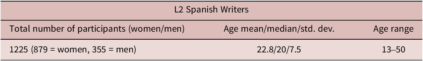
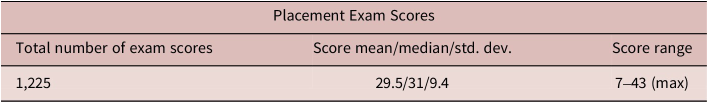
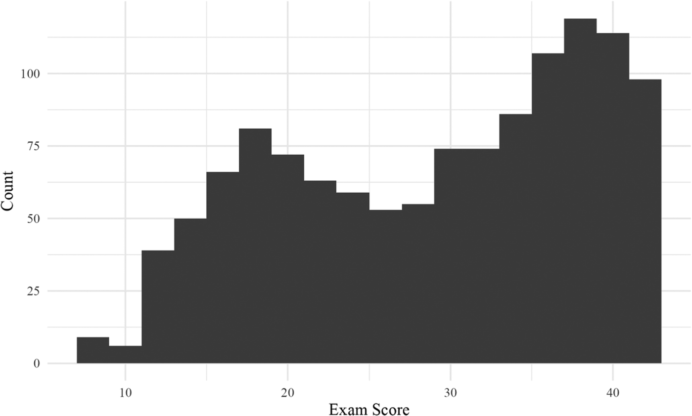
After these exclusions, 1,225 written responses remained for the statistical analysis reported below. Table 1 includes descriptive statistics for the L2 Spanish writers and Table 2 displays the descriptives for the placement exam scores. Figure 1 represents a histogram of the scores, which have a first quartile of 21 and a third quartile of 38.
Descriptive Statistics for L2 Spanish Writers

Descriptive Statistics of Placement Exam Scores

Distribution of exam scores.

University of Wisconsin Spanish Placement exam
Several scholars in applied linguistics (e.g., Thomas Reference Thomas, Norris and Ortega2006; Tremblay Reference Tremblay2011; Al-Hoorie & Vitta Reference Al-Hoorie and Vitta2019) have encouraged researchers in the field to more thoroughly operationalize their target constructs, particularly proficiency, and to ensure appropriate selection of measurement instruments and statistical models used to analyze the data generated by the measures (Plonsky, Reference Plonsky2015). As such, in this section we describe the nature of the writing sample collected from participants as well as the measure of language ability utilized in this study.
The response variable analyzed in the present study is the total number of correct responses per eligible participant on an early version of the language usage portion of the University of Wisconsin (UW) Spanish Placement Exam (University of Wisconsin, 1998). The exam is not proctored and can be accessed via a link to a Google Form found on the CEDEL2 website. Only the first of two sections of the full exam is given to CEDEL2 participants, which includes 43 closed-response, multiple-choice items focused on language usage, i.e., lexico-grammar (see Appendix 2 for sample items from the first section of the exam). The portion of the exam completed by participants does not include constructed responses, nor any items testing aural (i.e., listening) comprehension.
Though it was originally designed to place students in the UW system and not as a proficiency exam, the creators of CEDEL2 have used it as a rough measure of participants’ Spanish lexico-grammatical ability. The creators of the placement exam aimed to assess “knowledge of proper language usage.”Footnote 4 Though the word proficiency has been used by the CEDEL2 creators on their website to describe the construct these 43 items are assessing, we have chosen to define the construct more narrowly as receptive lexico-grammatical ability, that is, the ability to identify the ways in which grammatical structures establish relationships between lexical items and functors such that meaning can be accurately extracted from a written text by a language user (see Halliday & Matthiessen, Reference Halliday and Matthiessen2014 for an in-depth treatment of the construct from a functionalist approach). We recognize that this is only one of many constructs that constitute Bachman and Palmer’s (Reference Bachman and Palmer1996) conceptualization of language knowledge within the larger construct of language ability. To construct a defensible validity argument for the use of this instrument in the current context, we present two pieces of evidence for consideration: (1) students’ self-assessments of their overall Spanish proficiency highly correlated with the 43-item UW Spanish Placement Exam scores (r = .735, p <.001), (2) all our measures of LD significantly predicted exam score such that more LD in the writing task predicted higher language usage exam scores, demonstrating the positive relationship between LD and measures of language ability. This finding aligns with previous research that has noted a positive relationship between learners’ performance on the 43-item UW Spanish Placement Exam and other measures of language ability, such as lexical and lexico-grammatical ability (Consolini & Kyle, Reference Consolini and Kyle2024) and differential object marking (Simon, Reference Simon2022).
To give the reader a sense of the differences in writing ability among the writers, three sample responses are given in Appendix 1. Sample 1 was composed by a writer with a low score of 13 out of 43 (30%) on the placement exam, sample 2 was written by a writer who scored 25 out of 43 (58%), while sample 3 was written by a writer who received a high score on the exam: 40 out of 43 (93%). Each of the participants responded to Prompt 4: ¿Qué hiciste el año pasado durante las vacaciones? “What did you do last year during summer vacation?”. In order to protect the identity of the writers, we have anonymized personal information. To give a sense of the differences among the three samples, we reproduce here the first sentences of the three responses, accompanied by free translations: Durante las vacaciones, fue nadar a la de [Lugar]! “During vacation, I went swimming at [Place]!” (from Sample 1); En el año pasado me viajé en mexico con mi padre. “Last year I traveled in Mexico with my father.” (from Sample 2); Durante las vacaciones del verano, trabajé por una escuela internacional de lengua que se llama EF. “During summer vacation, I worked for an international language school that is called EF.” (from Sample 3). See Appendix 1 for the full sample responses.
Predictor variables
We analyzed eight LD measures, five socio-demographic variables, as well as text length. With the exception of TTR, we used LD measures that have been shown to be resistant to the text-length sensitivity effect described above, and we operationalized lexical items as orthographic word forms. Specifically, we analyzed: Maas’s a 2 measure (referred to below as simply Maas) (Maas, Reference Maas1972), Measure of Textual Lexical Diversity (MTLD-original), MTLD-MA-bidirectional, MTLD-MA-wrap (McCarthy & Jarvis, Reference McCarthy and Jarvis2010), Hypergeometric Distribution Diversity (HD-D) (McCarthy & Jarvis, Reference McCarthy and Jarvis2007), and Moving Average Type-to-Token Ratio (MATTR) (Covington & McFall, Reference Covington and McFall2010), as well as the first principal component of a PCA based on those six measures. In spite of its limitations as a reliable measure, we also analyzed TTR to serve as a basic benchmark against which to compare the other LD measures (Thomson & Thompson, Reference Thomson and Thompson1915). To be clear, we do not propose that TTR is a useful measure, but we use it here only to demonstrate the extent to which the other measures are more or less predictive.
In order to calculate the lexical diversity measures, we primarily used the lexical_diversityFootnote 5 Python module, with some exceptions. To calculate MTLD-MA-bidirectional, we made a slight modification to the implementation in lexical_diversity in order to reduce the run time by a factor of four, despite not changing the results. To calculate MTLD-MA-wrap, we wrote our own implementation based on Python code that Scott Jarvis, a co-creator of the algorithm, sent us, given the fact that the implementation in lexical_diversity did not return the exact same results, albeit that they were very similar, to what we expected, given Vidal and Jarvis’s (Reference Vidal and Jarvis2020) description of the algorithm.Footnote 6 To calculate Maas, we used the LexicalRichnessFootnote 7 Python module, as its implementation uses the natural logarithm, which is what Maas’s (Reference Maas1972, p. 78) formula specifies, while the implementation in lexical_diversity uses the logarithm to base 10. Admittedly, this difference is unimportant in practical terms, as the natural logarithm of numbers perfectly correlates with the logarithm to base 10 of those same numbers (r = 1.0).
In addition to lexical diversity, we analyzed the socio-demographic and socio-linguistic predictors found on the survey that were required of all contributors to the corpus, which included the age and genderFootnote 8 of the writers, the number of years studying Spanish, writers’ age at first exposure—i.e., “Age of exposure to L2 Spanish (AoE)”, and whether the writers had ever participated in a study abroad program.
Lexical diversity measures
Concerning the particular LD measures that we chose, the six measures of interest here (i.e., Maas, three MTLDs, HD-D, and MATTR) have been shown to be less affected by text length than other LD measures (e.g., TTR, Root TTR, Log TTR) and because these measures have been used previously in lexical diversity research, as mentioned above. Of interest here is the fact that these measures take different approaches to approximating the underlying construct of lexical diversity. All LD measures, including the original TTR measure, are fundamentally based on the difference between the number of word tokens (i.e., running words) and the number of word types (i.e., unique words). The LD measures make different use of the number of word types and the number of word tokens. To illustrate the difference between word tokens and word types, example (1) below contains 11 word tokens (i.e., running words) but only 10 word types (i.e., unique words) because muy “very/really” is repeated.
(1) La pelicula es muy interasante y los actores son muy bien. “The movie is very interesting and the actors are really good” (EN_WR_21_20_3_3_BB; the original text is left unaltered in this example).
In order to illustrate how the different LD measures make use of tokens and types, we detail the measures as follows. The original Type-to-Token Ratio (TTR) is the simple quotient of the number of word types divided by the number of word tokens. See Equation 1.
Equation 1. Type-to-Token Ratio (TTR)
 $$ TTR=\frac{N\; types}{N\; tokens} $$
TTR is highly negatively correlated with text length, because words are repeated more often as texts increase in length, and thus the denominator increases, driving down the quotient.
A simple remedy for the text-length sensitivity problem of TTR is to perform a non-linear mathematical transformation of TTR, and that is the approach of Maas. It is calculated by taking the difference between the logarithm of the number of tokens and the logarithm of the number of types and dividing that difference by the square of the logarithm of the number of tokens, as shown in Equation 2.
Equation 2. Maas’s a 2 lexical diversity measure
 $$ Maas\hbox{'}s\hskip0.4em {a}^2=\frac{\mathit{\log}\left(N\; tokens\right)-\mathit{\log}\left(N\; types\right)}{{\left(\mathit{\log}\left(N\; tokens\right)\right)}^2} $$
Another fairly simple remedy for the text-length sensitivity of TTR is to use equal-sized windows and calculate the mean TTR of all windows. This is the approach of the Moving Average Type-to-Token Ratio (MATTR). Specifically, the TTR of the first 50 words is calculated and stored, and then the TTR of the 50-word window from the second word to the 51st word is calculated and stored, and so forth until the end of the text is reached. Then, the mean TTR of all 50-word windows is calculated, and that mean is the MATTR of the text (Covington & McFall, Reference Covington and McFall2010).
While still fundamentally based on word types and word tokens, the hypergeometric distribution diversity (HD-D) measure takes a probabilistic approach. Specifically, HD-D is the summed probabilities of tokens of each word type being selected in a random sample without replacement of 42 tokens in the text (see McCarthy & Jarvis, Reference McCarthy and Jarvis2007 for details).
Like MATTR, the three MTLD measures take a windowed approach, but differ from MATTR by using a variable-sized window. The original MTLD is the “mean length of sequential word strings in a text that maintain a given type-to-token (TTR) value” (McCarthy & Jarvis, Reference McCarthy and Jarvis2010). That threshold TTR value is most often specified by researchers and software as 0.72.Footnote 9 The number of continuous, non-overlapping spans of words that have a TTR at or above the threshold value (i.e., 0.72) is calculated, and these spans are called factors. The partial factor at the end of a text (unless by extremely rare chance the text ends on a complete factor) is graded based on the distance where the TTR falls from 1.0 down to 0.72. Finally, the total number of words in the text is divided by the number of factors and the resulting quotient is the MTLD-original value for the text.
The MTLD-MA-bidirectional and the MTLD-MA-wrap measures are modifications of the MTLD-original. The MTLD-MA-bidirectional measure calculates the MTLD of the text starting from the beginning of the text and moving to the end of the text, as is the case with MTLD-original. Then, the MTLD of the text is calculated starting at the end of the text and moving backward to the beginning of the text. Then, the two MTLD scores (i.e., beginning-to-end, end-to-beginning) are averaged and the result is the MTLD-MA-bidirectional score for the text. While highly correlated, MTLD-MA-bidirectional is not perfectly correlated with MTLD-original.
The MTLD-MA-wrap is another modification of MTLD-original. The difference between this metric and MTLD-original is that, instead of calculating a partial factor at the end of the text as with MTLD-original, the MTLD-MA-wrap algorithm wraps around to the beginning of the text once the end of the text has been reached, and keeps calculating TTRs until the final factor has been completed (i.e., the TTR of the final window drops below .72). Then, the average number of words in the factors is calculated and that number is the MTLD-MA-wrap for the text. Like with MTLD-MA-bidirectional, MTLD-MA-wrap is highly correlated with MTLD-original, but not perfectly correlated with it.
As mentioned above, we created a composite LD score based on PCA. Specifically, we entered into a PCA the six previously mentioned LD measures other than the original TTR, that is, Maas, MATTR, HD-D, MTLD-original, MTLD-MA-bidirectional, and MTLD-MA-wrap. PCA is a dimensionality reduction algorithm that identifies and re-references data by linear mapping and transforms correlated variables into components, which are themselves uncorrelated. As Crawley (Reference Crawley2013, p. 810) states: “the aim is to find linear combinations of a set of variables that maximize the variation contained within them, thereby displaying most of the original variation in fewer dimensions.” The resulting first principal component captures the largest amount of the variability in the variables, while the second principal component captures the second largest amount, and so on. With intercorrelated variables like lexical diversity measures, PCA offers a useful way to boil down, so to speak, these intercorrelated variables into fewer meaningful variables. By and large, the first component of a PCA explains the vast majority of the variability, and it is this component that we use as a composite LD measure. It may be desirable to create a composite measure that ameliorates weaknesses among individual LD measures, and this study explores the extent to which one such composite measure is a better predictor of L2 ability than individual measures.
Table 3 offers a summary of the calculation of the LD measures used in this study.
Summary of Calculations of LD Measures Used in This Study

Pre-processing of L2 data
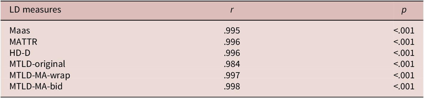
Before calculating the LD measures, we performed two preprocessing steps. First, we checked for spelling errors by applying the Hunspell spell checkerFootnote 10 to the written responses in an automated fashion with a Python script that we wrote. Spelling correction is a fairly standard pre-processing step in automated processing of learner corpora because many tools (e.g., taggers, LD analyzers, syntactic complexity analyzers) are trained on or designed for L1 data with far fewer spelling errors than typically exists in L2 corpora (see Callies, Reference Callies, Granger, Gilquin and Meunier2015 for more discussion of handling errors in automated processing of L2 data). If Hunspell suggested a spelling correction, our Python script made the change, for example: *resturante > restaurante ‘restaurant’, *musica > música ‘music’, *tabacco > tabaco ‘tobacco’, *bastnate > bastante ‘enough’, *intilligete > inteligente ‘intelligent’. On the contrary, if Hunspell indicated a spelling error but did not offer a suggested correction, our script did not make a change. It should be noted that some of the spelling problems detected by Hunspell were English words. For example, the following spelling “errors” were changed by Hunspell to the words to the right of the arrows: plane > plena ‘full’, degree > negree ‘3s blacken’, fool > fol ‘abbreviation of folio’, seasons > easonense ‘demonym of San Sebastián, Spain’. Despite the fact that these spelling corrections are not accurate, they likely have a negligible effect on the LD scores of the texts. For example, whether a given LD measure receives the correct word for English plane, that is, Spanish avión, or an incorrect change to plena ‘full’ doesn’t change the fact that the LD measure sees one token of a unique word type. While we admit that ideally each text could be examined manually by a human to ensure accurate spelling corrections made by Hunspell, we speculate that the effect of uncorrected spelling errors, incorrectly changed spelling errors, and changed English words is minimal on our results. In order to test this assumption, we randomly selected 40 written responses, ten from each of the four quartiles along the range of placement exam scores, that is, ten random responses each from the following exam score ranges: 7–21, 22–31, 32–38, 39–43. Next, we manually corrected spelling errors in those 40 responses and then reran our script to calculate the LD metrics, without using Hunspell. Finally, we calculated Pearson’s r correlation coefficients for each of the six LD measures of interest here, using the 40 manually corrected responses and their corresponding Hunspell-corrected versions. The results show that the correlation coefficients between the manually corrected responses and their Hunspell-corrected versions are above r = .98, suggesting near-perfect correlation. See Table 4.
Correlation between Manually Corrected and Hunspell-Corrected Versions of 40 Randomly Selected Responses

The second pre-processing step we performed was to tokenize the spell-checked text in such a way that punctuation was removed, as LD analysis concerns the lexis, not the punctuation, of a language. We wrote a regular expression tokenizer function in Python to perform this pre-processing step, with the body of the function in Snippet 1:
Snippet 1. Python code to tokenize text and remove punctuation
tokens = re.findall(r"[-a-záéíóúüñ]+", text.upper(), flags = re.IGNORECASE)
Statistical model
Our initial analysis included a series of mixed-effect linear regression models, one model per LD measure along with the other predictors (i.e., age and gender of speaker, whether they studied abroad, etc.). However, upon checking the assumptions of those models, we discovered heteroscedasticity when viewing the scatterplot of the residuals by the fitted values of each linear model. Figure 2 shows the plot from the model that included MATTR with other predictors. The scatterplots of residuals by fitted values of the other models look very similar and also strongly suggest heteroscedasticity.
Residuals by fitted values of mixed-effect linear regression model with MATTR and other predictor variables.

Because the assumption of homoscedasticity of linear regression modeling is not met in our data, we opted for mixed-effects logistic regression models, as logistic regression does not have the assumption of homoscedasticity. The response variable in our logistic regression models is the number of correct responses versus incorrect responses on the UW Spanish Placement Exam. The predictor variables include those described above, with only one LD measure per model. For example, the model with MTLD-MA-wrap included that particular LD measure along with text length, age and gender of writers, years of exposure to Spanish, age of first exposure to Spanish, whether the writers had ever studied abroad, and writing prompt as a random intercept. Because previous research has shown that writing prompt or task type can affect L2 LD (e.g., Ansarin et al., Reference Ansarin, Karafkan and Hadidi2021), we chose to control for this factor because we were primarily interested in making predictions across task types. Also, we standardized the scale of all continuous predictors by calculating z-scores. The R code in Snippet 2 gives the model formula for a sample model, the one with MATTR.
Snippet 2: R code of sample regression model
lme4::glmer(formula = cbind(exam_score, 43 - exam_score) ~ scale(n_wds) * scale(mattr) + scale(age) + scale(yrs_study) + scale(age_exposure) + gender + study_abroad + (1|prompt), data = cedel, family = binomial, nAGQ = 0)
Concerning model comparison, in a frequentist (i.e., null-hypothesis) statistical framework, only nested models can be compared with ANOVA in order to calculate p-values for comparison purposes. Differently, in a Bayesian statistical framework, Bayes factors can be used to perform model comparison with both nested and unnested models. Including the model with the first principal component (PC1) from the PCA, we have eight unnested models that are identical aside from the LD measure of the moment: model 1 with the original TTR, models 2–7 with the six text-length-corrected measures (i.e., Maas, MATTR, HD-D, MTLD-original, MTLD-MA-bidirectional, MTLD-MA-wrap), and model 8 with PC1 that is based on the six text-length corrected measures. Consequently, we used Bayes factors to compare the models. We specified the model with the original TTR measure as the baseline model against which the other seven models were compared. Rather than answering the question that is asked in the frequentist framework, that is, “How probable are the observed data if the null hypothesis were true?”, we use Bayes factors to answer the question: “Under which model are the observed data more probable?” Given the data at hand, the Bayes factors indicate the relative evidence of one model over another, or in other words, how much more or less probable the current model is in comparison to the baseline model. We used the bayesfactor_models function in the bayestestR R package to calculate the Bayes Factors (cf. Makowski et al., Reference Makowski, Ben-Shachar and Lüdecke2019).Footnote 11
Results
Logistic regression models
The results of a series of logistic regression models show that each of the LD measures (i.e., Maas, MATTR, HD-D, MTLD-original, MTLD-MA-bidirectional, MTLD-MA-wrap, PC1 based on those previous six measures, as well as TTR) significantly predicts the number of correct responses on the placement exam taken by the writers, at an alpha level of p = .05. The eight models have similar results: the interaction term between text length and the LD measure of the given model was selected as significant. Also selected as significant were the following other predictor variables: the age of the speaker, whether the speaker had ever studied abroad, and the number of years studying Spanish. Four of the seven models (i.e., the one with Maas, the one with MATTR, the one with MTLD-original, and the one with TTR) selected the age of exposure to Spanish as significant. No model selected the gender of the speaker as predictive. The random effect of prompt also showed little variance in each model, so we choose not to consider it further here. As the models are similar to each other, we will examine one model here as an illustrative model. Table 5 displays the results of the model with MTLD-MA-wrap as a predictor variable. All models are presented in Appendix 3.
Logistic Regression Model with MTLD-MA-Wrap

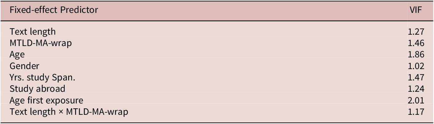
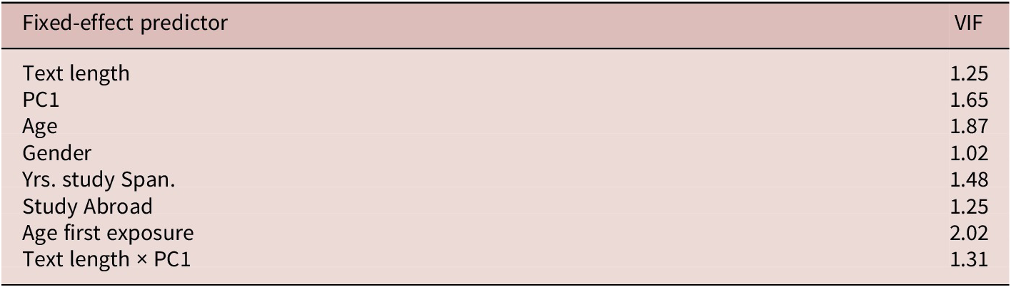
Concerning the assumption of logistic regression that the predictors are not multicollinear, the Value Inflation Factors (VIF) suggest that this assumption is met, as the VIFs of this model are at or below a value of 2.01. See Table 6.
Value Inflation Factor Scores of Logistic Regression Model That Included MTLD-MA-Wrap

As mentioned above, the interaction term between text length and MTLD-MA-wrap was selected as a significant predictor, and thus we immediately turn our attention to it. In order to visualize this significant interaction, Figure 3 splits the continuous variable of text length into an ordinal categorical variable with three equal-size bins based on number of observations: short texts with between 50 and 167 words, mid-length texts with between 168 and 437 words, and long texts with between 438 and 1,297 words. To be clear, we divide text length into an ordinal categorical variable here only to visualize the interaction, while in the regression reported in Table 5 above, text length was entered as a continuous quantitative variable. In each of the scatterplots in Figure 3, the dots represent individual texts, the x-axis represents the MTLD-MA-wrap scores, and the y-axis represents the writers’ scores on the placement exam. See Figure 3.
Exam score by MTLD-MA-wrap by binned text length.

As seen in the figure, MTLD-MA-wrap positively correlates with exam score such that as MTLD-MA-wrap increases, exam score increases too. However, the effect is variable, as the correlation is weakest in the short texts in the left-hand scatterplot and strongest in the long texts in the right-hand scatterplot. Specifically, the slope of the regression in the short texts (left-hand) scatterplot in Figure 3 is .11 (r = .26), while the slope of the regression line in the mid-length texts (center) scatterplot is .16 (r = .45), and the slope in the long texts (right-hand) plot is .18 (r = .48).
The other factors that significantly predict exam score are age of speaker, years studying Spanish, and study abroad participation. Concretely, exam scores increase as the age of writers increases and as the number of years studying Spanish increases. Additionally, writers who had studied abroad scored higher on the placement exam than writers who had not participated in such a program. Again, the results of all the models are reported in Appendix 3.
Principal component analysis
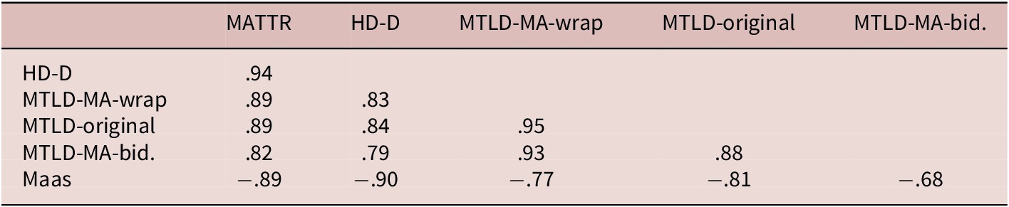
In order to create a composite score of LD, we entered into a PCA the six measures that have been shown to be resistant to the text-length effect (i.e., Maas, MATTR, HD-D, MTLD-original, MTLD-MA-bidirectional, MTLD-MA-wrap). First, we calculated the pairwise Pearson correlation coefficients of the six measures, as variables should be correlated to be entered into a PCA. As expected, the six LD measures are highly correlated, with coefficients ranging from .82 to .94. See Table 7.
Pearson Correlation Coefficients of Six LD Measures

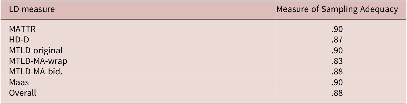
We also checked the sampling adequacy of the LD measures and found that three measures have marvelous sampling adequacy (i.e., between .9 and above) and three measures have meritorious sampling adequacy (i.e., between .8 and .89) (see Field et al., Reference Field, Miles and Field2012; Hutcheson & Sofroniou, Reference Hutcheson and Sofroniou1999; Kaiser, Reference Kaiser1974). See Table 8.
Kaiser-Meyer-Olkin Sampling Adequacy Scores of Five LD Measures

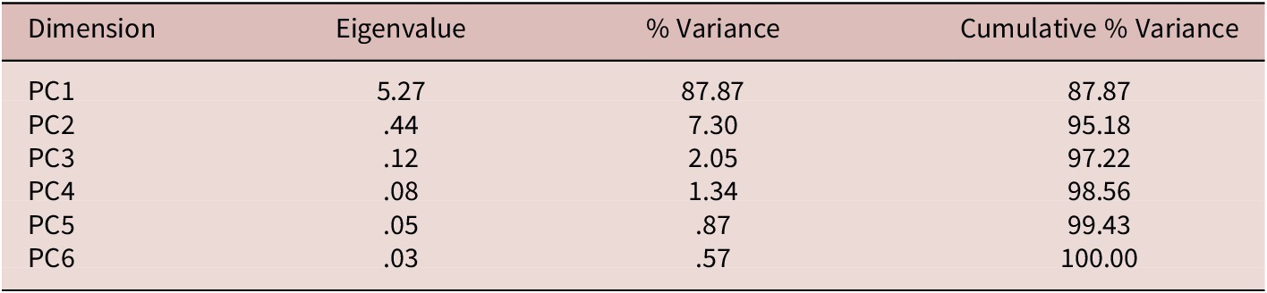
The PCA results find that the first principal component (PC1) accounts for 87.9% of the variance and has an eigenvalue of 5.27, while the second PC accounts for only 7.3% of the variance, with an eigenvalue of .44. Using the Kaiser Criterion (i.e., eigenvalue > 1.0), we retain only the first PC (see Kaiser, Reference Kaiser1974) for further analysis. See Table 9.
Eigenvalues and Percentage of Explained Variance of Principal Components

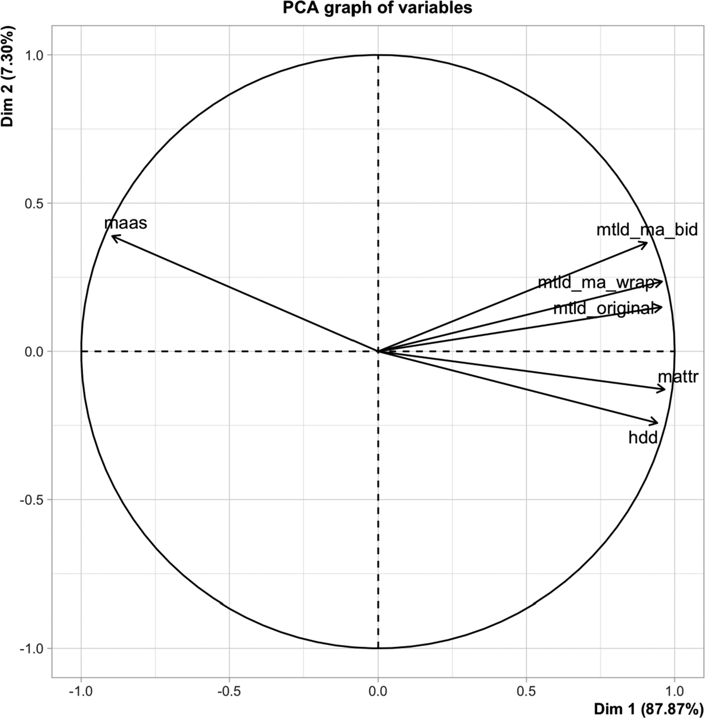
In order to analyze to what degree the LD measures load onto PC1, we drew a vector plot, as seen in Figure 4. The smaller the angle between a variable’s vector and the PC (or Dimension), the stronger the correlation. As seen, all six LD measures load onto PC1 (i.e., “Dim 1” in the figure). The lengths of the vectors indicate how much variation is accounted for on the plane, with a maximum of 1.0 (the circle). As seen, the variation in these six LD measures is almost completely accounted for on the plane because their vectors nearly touch the circle. See Figure 4.
Vector plot of PCA.

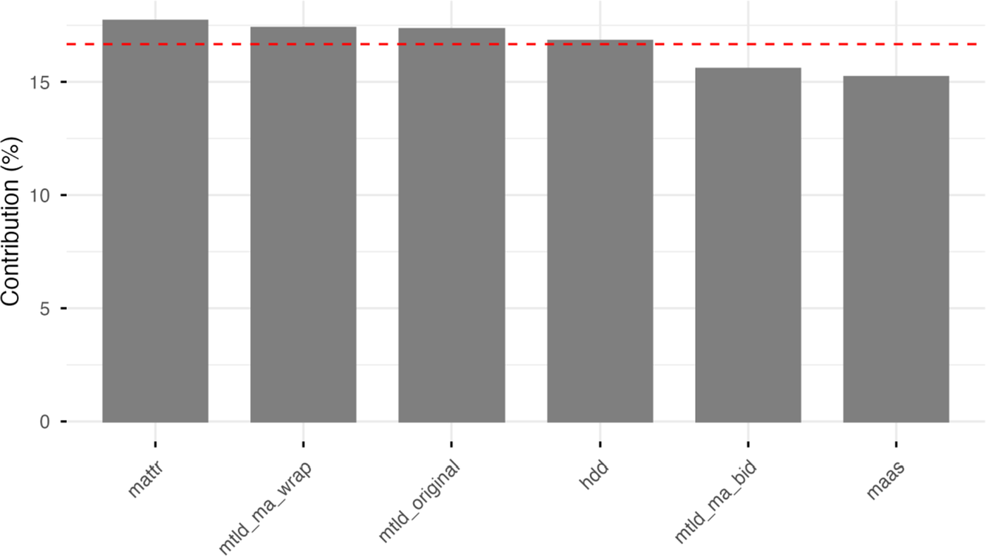
All six LD measures contribute similarly to PC1, each contributing between approximately 15% and 18%. See Figure 5.
Contribution of six LD measures to PC1.

Next, we entered PC1 into a logistic regression as a composite LD measure, along with the other predictor variables noted above (e.g., age and gender of speaker, participation in study abroad, etc.). Like the other LD measures in their respective regression models, PC1 significantly predicts exam score in its regression model. See Tables 10 and 11.
Mixed-Effect Logistic Regression with PC1 Along with Other Predictors

Value Inflation Factor Scores of Logistic Regression Model That Included PC1

As was the case with the other LD measures, the interaction term between text length and PC1 significantly predicts exam score, and thus we turn our attention to that interaction. Similar to Figure 3 above, we divided text length into three bins for visualization purposes only in order to elucidate the interaction between that text length and PC1. But again, in the regression itself, text length was entered as a continuous quantitative variable. Figure 6 shows that the effect of PC1 is greatest in the mid-length texts (between 168 and 437 words in length) and long texts (between 438 and 1,300 words) and weakest in short texts (between 50 and 167 words). The x-axis of each scatterplot represents the first principal component while the y-axis represents the writers’ scores on the placement exam. See Figure 6.
Exam score by PC1 by text length.

Model comparison
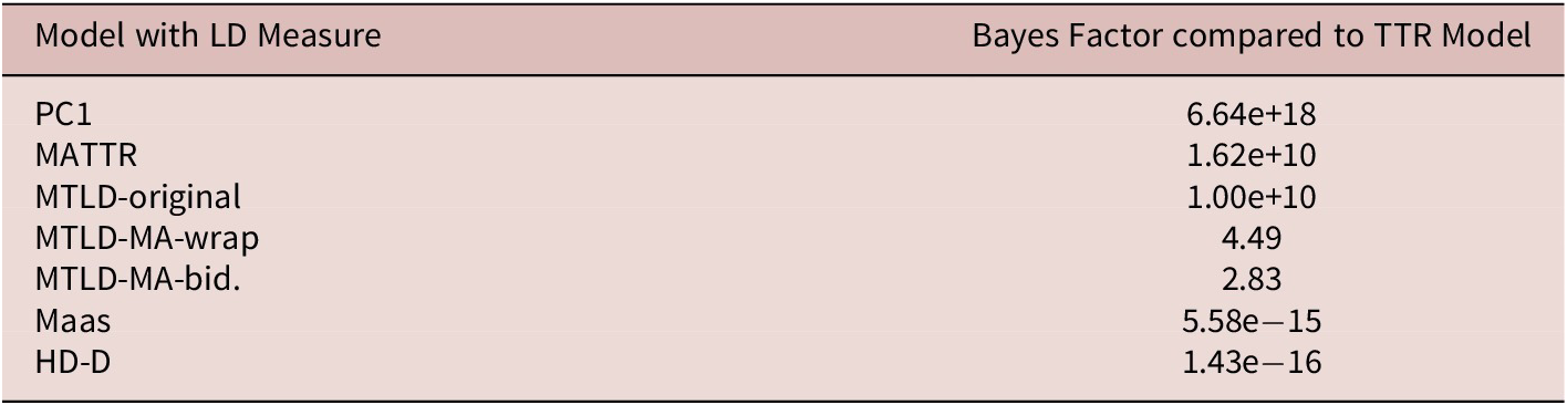
As mentioned above, we used Bayes Factors to compare the models. Table 12 displays the Bayes Factor for each model in comparison to the baseline model with the original TTR measure. The rows of the table are arranged in descending order, with the most probable model first. See Table 12.
Bayes Factors for Model Comparison

With a Bayes Factor of 6.64e+18, the model with PC1 is the favored model, or in other words, the model under which the observed data are most probable in comparison to the model with TTR. Specifically, the model with PC1 is 6.64e+18 times more probable than the model with TTR. The next two models have fairly similar Bayes factors: the model with MATTR has a Bayes factor of 1.62e+10, while the model with MTLD-original has a Bayes factor of 1.00e+10. The next two models have Bayes factors that are much lower in the hierarchy: the model with MTLD-MA-wrap with a Bayes factor of 4.49, and the model with MTLD-MA-bidirectional with a Bayes factor of 2.83. Finally, two models had Bayes Factors below 1.0, and thus these two models are dispreferred in comparison to the model with TTR: the model with Maas has a Bayes factor of 5.58e−15, and the model with HD-D has a Bayes factor of 1.43e−16. To summarize, the model with PC1 is the most probable model, by far, when all models are compared to the one with TTR.
Discussion
The first research question (i.e., RQ1) asked which individual LD measure or measures best predict receptive lexico-grammatical ability in written L2 Spanish. Reviewing the Bayes Factors reported in Table 12 above, we see that among the six LD measures that are resistant to the text-length sensitivity effect (i.e., Maas, MATTR, HD-D, MTLD-original, MTLD-MA-wrap, MTLD-MA-bidirectional), two measures closely group together near the top of the hierarchy: MATTR and MTLD-original. As a result, we offer the following answer to RQ1: while MATTR (Bayes factor: 1.62e+10) is slightly favored in comparison to MTLD-original (1.00e+10), the difference is minimal, and consequently we suggest that, in practical terms, any one of these two measures is useful for predicting receptive lexico-grammatical ability in L2 Spanish writing in our dataset. Two other measures (i.e., MTLD-MA-wrap: 4.49, MTLD-MA-bidirectional: 2.83) fall further down in the hierarchy of Bayes factors, and thus we suggest that they are less effective at predicting this particular language ability in these data with lexical items operationalized as orthographic forms. At the bottom of the hierarchy are Maas and HD-D, whose Bayes Factors (5.58e−15, 1.43e−16, respectively) fall below one, which suggests that in these data, the model with Maas and the model with HD-D are less probable than the baseline model with TTR.
The second research question (i.e., RQ2) asked whether a composite LD score based on PCA better predicts lexico-grammatical knowledge in written L2 Spanish than does any single LD measure. The Bayes Factors clearly favor the model with the composite score (i.e., PC1: 6.64e+18), and thus this research question can be answered affirmatively. Consequently, while any one of the two modern LD measures near the top of the hierarchy of Bayes factors (i.e., MATTR and MTLD-original) might accurately predict learners’ language ability tested by the placement exam, the results from our data suggest that creating a composite LD score based on PCA better predicts lexico-grammatical ability than any single LD measure, including MATTR and MTLD-original. These results seem to contradict our answer to the first research question: in these data, there is a single best LD measure, and that measure is the first principal component of a PCA based on the six LD measures tested here. That said, we immediately point out that this paper is a first foray into creating a composite LD score based on PCA in L2 Spanish. To be clear, we did not perform an exhaustive analysis of different combinations of LD measures in PCAs; rather, we used six specific LD measures cited in the literature as being resistant to the text-length sensitivity effect. Whether there is a better combination of LD measures that would create an even stronger composite measure based on PCA score falls outside the scope of this paper and future research will have to take up such an exhaustive analysis. Also, whether a composite LD index based on PCA is resistant to the text-length sensitivity problem discussed above should be taken up in future investigations.
The results of the current study concur with the large body of literature showing a positive relationship between LD and language ability (Crossley et al., Reference Crossley, Salsbury, McNamara and Jarvis2011, Reference Crossley, Salsbury and McNamara2012; Crossley & McNamara, Reference Crossley and McNamara2012; Gebril & Plakans, Reference Gebril and Plakans2016; e.g., Jarvis, Reference Jarvis2002; Kyle et al., Reference Kyle, Crossley and Jarvis2021; Lee, Reference Lee2019; Loomis, Reference Loomis2015; Malvern et al., Reference Malvern, Richards, Chipere and Durán2004; Matsumoto, Reference Matsumoto2010; Treffers-Daller et al., Reference Treffers-Daller, Parslow and Williams2018; Woods et al., Reference Woods, Hashimoto and Brown2023; Yu, Reference Yu2010). As expected, in our data, LD is positively correlated with receptive lexico-grammatical ability, as assessed by the placement exam. Our results also contribute to the literature about the relationship between LD and L2 ability in languages other than English (Gharibi & Boers, Reference Gharibi and Boers2019; Hržica & Roch, Reference Hržica, Roch, Armon-Lotem and Grohmann2021; Sung et al., Reference Sung, Cho and Kyle2024), and in particular L2 Spanish–an inflectionally rich language (Castañeda-Jiménez & Jarvis, Reference Castañeda-Jiménez, Jarvis and Geeslin2013; Consolini & Kyle, Reference Consolini and Kyle2024; Fernández-Mira et al., Reference Fernández-Mira, Morgan, Davidson, Yamada, Carando, Sagae and Sánchez-Gutiérrez2021; Schnur & Rubio, Reference Schnur and Rubio2021; Tracy-Ventura et al., Reference Tracy-Ventura, Huensch, Mitchell, Le Bruyn and Paquot2021). As noted above, in their study using the same corpus utilized here, Consolini and Kyle (Reference Consolini and Kyle2024) found a positive relationship between receptive lexico-grammatical ability and LD, mean frequency of words per text, and bigram association as measured with the delta P (ΔP) metric. Likewise, Schnur and Rubio (Reference Schnur and Rubio2021) found a positive correlation among K-12 dual immersion Spanish learners between proficiency level on the ACTFL guidelines scale and several lexical measures, including LD, lexical sophistication, and lexical density.
Our results also contribute to the conversation in the literature on the usefulness of LD measures that have been proposed to ameliorate the text-length sensitivity effect that is so prevalent with previous measures, and in particular with the traditional TTR measure. As mentioned above, Zenker and Kyle (Reference Zenker and Kyle2021) show that MATTR and two MTLD measures are stable, and therefore useful, with texts of disparate lengths. This plays out in our data too, as MATTR and MTLD-original are highly predictive of language ability and are near the top of the hierarchy of LD measures, despite the fact that the texts in our data vary in length.
The results of this paper also contribute to the conversation about which might be the best LD measure to use with L2 language data. Our results seem to suggest that, among the already existing LD measures, there may not be only one best LD measure. As explained above, two measures, that is MATTR and MTLD-original, were similarly useful in predicting language ability in L2 Spanish in these data. Consequently, rather than trying to identify only one best LD measure, researchers are likely better served by making use of a handful of LD measures. As mentioned previously, researchers have found varying levels of usefulness of LD measures (cf. Bestgen, Reference Bestgen2024 for an overview of many LD measures). These results concur with the takeaway of Woods et al. (Reference Woods, Hashimoto and Brown2023): it is probably best to use multiple LD measures when studying L2 interlanguage. This is the case when studying languages other than English, the L2 language that is most represented in previous studies.
A novel finding of our analysis is that the first principal component of a PCA based on the six LD measures studied here better predicts receptive lexico-grammatical ability in written L2 Spanish than does any one of those already established LD measures. Consequently, this finding gives nuance to our previously mentioned conclusion, that is, in addition to using a handful of LD measures with L2 language, it is useful to create a composite LD score based on PCA. This finding builds on the impressive work of previous researchers who have created sophisticated LD measures (Bestgen, Reference Bestgen2024; Jarvis, Reference Jarvis2013; McCarthy & Jarvis, Reference McCarthy and Jarvis2010; Treffers-Daller, Reference Treffers-Daller, Jarvis and Daller2013) in an effort to control for the text-length sensitivity problem.
This research makes no claims about how L2 lexical knowledge is represented in the learner’s lexicon, how L2 Spanish lexical items are acquired, nor how they should be taught. The primary contribution of this study is methodological and should prove helpful for researchers seeking useful and valid tools for measuring lexical diversity of a given L2 Spanish text, regardless of the specific research question. More concretely, researchers in L2 lexis have additional evidence that: (1) LD measures predict well constructs of language ability such as receptive lexico-grammatical ability, and (2) a composite score that combines various LD measures may provide the most accurate and reliable indication of how lexically diverse an L2 text is. Researchers will, of course, carefully consider which instruments best serve their unique research questions and context, but this research has given them useful information upon which to base their decisions.
Conclusion
The question of which, if any, LD measure best predicts receptive lexico-grammatical ability in written L2 Spanish is analyzed in this study. A total of 1,225 written responses to 14 prompts from the CEDEL2 corpus of written L2 Spanish were utilized. In addition to written responses, the writers took a 43-point receptive lexico-grammatical Spanish exam created at the University of Wisconsin, and their score was used as a proxy for language ability. The results of our analysis suggest that a composite LD score based on PCA of six LD measures best predicts receptive lexico-grammatical language ability in these data.
Turning to limitations of the current study, one potential limitation is our operationalization of the lexical unit. As mentioned above, Jarvis and Hashimoto (Reference Jarvis and Hashimoto2021) found that the operationalization of the lexical unit was a non-trivial step in their study of narrative texts written by adolescent L1 and L2 writers, finding that lemmas or word families were the lexical unit that best corresponded to human judgments of LD. However, their study focused on English, and future researchers would do well to explore the effect of different operationalizations of the lexical unit in Spanish, a language with a rich inflectional morphology, and in other languages. Additionally, although it is a standard step for automated processing of learner data, it is also not entirely known how spell checking affects the results of LD in learner corpora generally. Another limitation of the current paper is the fact that only eight LD measures were used: the six ones selected here that are resistant to the text lenght effect (i.e., Maas, MATTR, HD-D, MTLD-original, MTLD-MA-wrap, MTLD-MA-bidirectional), the traditional TTR, and a composite score based on PCA. There are others that could have been included as well (e.g., MSTTR, vocd-D, Root TTR, Log TTR). Future studies would do well to perform an exhaustive analysis of more LD measures.
Another avenue for future research is to analyze the usefulness of a composite LD score in oral L2 data. Kyle et al. (Reference Kyle, Sung, Eguchi and Zenker2024) analyzed the reliability and validity of a handful of LD measures in oral data and found that Root TTR, vocd-D, and HD-D lack reliability across texts of different lengths. However, they find reliability across different oral text lengths for “optimized” versions of MATTR and MTLD, that is, when MATTR is measured with a window span of 11 words rather than the usual 50 words, and MTLD is based on a TTR threshold of .92 rather than the usual .72. Future research might utilize different window spans of MATTR and different TTR thresholds of MTLD in order to investigate whether a composite LD score based on PCA with these measures is useful in oral L2 data.
Finally, PCA is just one of many methods of addressing multicollinearity and reducing dimensionality. PCA has been criticized for overfitting to data, limiting its generalizability to other data (e.g., Lippitt et al., Reference Lippitt, Carlson, Arbet, Fingerlin, Maier and Kechris2024). Future research should assess whether other methods, such as factor analysis, would be better suited for this kind of approach to LD measurement. An additional limitation with the use of PCA more generally is that in order to create a composite LD score based on PCA, researchers must have some computer programming ability. Currently, we know of no user-friendly software that performs such a calculation on a handful of LD measures, and this hurdle may prove insurmountable for some researchers or research teams.
Data availability statement
The experiment in this article earned Open Data and Open Materials badges for transparent practices. The data files and R code used in this study are available on OSF: https://osf.io/rwg4a/overview.
Competing interests
The authors declare none.
Appendices
Appendix 1: Sample written responses
Sample response 1:
Durante las vacaciones, fue nadar a la de [Lugar]! Fue con cinco ninos por a la fiesta. De ninos es muy bien. Fue to [Ciudad] y fue no bien. Yo como poison. Es mal! [Amiga] y mi como a la fiesta. Cervaza y vino es favorita. Trabajo a mi padres place, de convent, y lipriar de plant, y simpre mirror ninos. Mi vacaciones consisto Alaska, Africa, y Virginia! Yo trabaja en clasa y accepto en [Universidad]! [Universidad] es en [Ciudad], [Estado]. Yo completa mi educacion a [Universidad] en dos ayer. Yo studios consisto Occupational Therapy y Massage Therapy. No Espanol por mi!!! Yo no comprenda!
Sample response 2:
En el año pasado me viajé en mexico con mi padre. Era un buen tiempo. Y quiero hacerlo este verano tambien. La vaccacíon empezó en el avion. No fue una vuelo muy larga, solomente 3 o 4 horas. Nosotros aterrizemos en Puerto Vallarta y halló un taxi. Hacía buen tiempo todo tiempo. Todo era verde. Mi padre decedícte que el quiere pescar. Los pescados era muy grande y era muy defícil para obtenerlos. Una noche yo fue al un club. Los chicas eran guapas pero no muy simpaticos. La musica era muy alta y me duele mis orejas. Yo quiero ir al Mexico pronto y quedarme por mas tiempo.
Sample response 3:
Durante las vacaciones del verano, trabajé por una escuela internacional de lengua que se llama EF. Hay various escuelas de EF por todo el mundo, pero la escuela donde yo trabajaba está en [Ciudad]. A mi me encanta a [Ciudad]. Es una ciudad divertísima y nunca se aburre. También es una ciudad muy antigua, pues, antigua en relación a otras ciudades estados unidenses. Hay tanta historia allí y me gustaba leer las placas que contaban lo que pasó en un sitio o quien vivía allí hace 150 años. Yo vivía con mi novio, [Nombre]. Cada fin de semana, ibamos al mercado de [Calle] para comprar verduras. Entonces, caminabamos por la ciudad. A veces, jugabamos en el parque como si fuéramos niños. Un día fuimos a la playa y yo tomé demasiado sol. Al principio, era un poco extraño vivir juntos como una pareja casada. Teníamos que limpiar, cocinar, y ir de compras, con nuestro propio dinero! ¡Qué lástima! Como progresaba el verano, me acostumbraba a nuestra situación y ahora, creo que era uno de los mejores veranos de mi vida. Fui a [Ciudad] por dos razones. Primero, quería vivir con mi novio. Regresé de España en Mayo y no lo había visto desde Marzo cuando él me visitó. Necisitábamos recuperar el tiempo perdido. Además, quería seguir viviendo la vida urbana. Estoy de un pueblecito y no hay nada allí que compare con el carácter de la ciudad. La verdad es que el trabajo era bastante aburrido, pero nostoros sabíamos gozarnos. Encontré con amigos muy divertidos y etso hacía que los días eran soportables. Todavía hablo con ellos. Puesto que la escuela era una escuela de lengua, había muchos estudiantes de todos partes del mundo. Me gustaba encontrarlos y aprender also sobre sus países y lenguas. Lo mejor eran los estudiantes que hablaban español porque podía practicar la lengua con ellos, aunque era prohibido. Nico, mi estudiante favorito era argentino y antes de salir, me dio los restos de su mate, la bebida tradicional de Argentina. Me alegría que hubiera podido compartir cuentos y risas con mis nuevos amigos internacionales. Quedé a [Ciudad] por 12 semanas. Al regresar a mi hogar en [Estado], mi familia y yo fuimos de vacación. Visitamos la familia de me padre en [Estado]. Mi abuela vive en [Ciudad], donde el sol siempre brilla. No la había visto desde mi graduación de la escuela secondaria haces cuatro años. Nadamos en la piscina y Mee-Mee nos dio bebidas para emborracharnos. Ella era muy feliz al vernos dado que normalmente se ha sentido muy sola desde el muerto mi abuelo hace dos años. Yo la amo tremendemente y me da pena verla triste. Espero que ella pueda enamorarse a alguien de nuevo. Cuando piense del verano, no creo que haya occurido. Tenía todo que querría: el amor de mi novio, la emoción de una vida urbana, y, sobre todo, tiempo con mi familia.
Appendix 2: Sample UW Placement Exam Items
–¿Te costó mucho el libro? -- Sí, pagué veinte dólares ___ este libro.
-
a. Para
-
b. por
Nadie nos lo había dicho antes, pero anoche ___ la noticia de su muerte.
-
a. Supimos
-
b. conocimos
X: Mi tío tenía un coche muy bonito.
Y: ¿De qué color?
X: ___ rojo y negro.
-
a. Era
-
b. Fue
-
c. Estaba
-
d. Eran
Cuando yo ___ joven, fui a Chile.
-
a. Fue
-
b. Soy
-
c. era
-
d. fui
Como me gusta ayudar a otras personas y tengo bastante tiempo libre, ___
-
a. Estoy
-
b. Tengo
-
c. soy
voluntaria en un hospital muy grande de la ciudad de Milwaukee. A veces es muy agradable ___
-
a. Trabajo
-
b. Trabajar
-
c. trabajando
allí, pero tambien, de vez en cuando, tenemos problemas con ___ paciente majadero
-
a. Algún
-
b. Alguna
-
c. alguno
y con ciertos doctores arrogantes que se creen muy importantes. Con frecuencia, para ___ el tiempo, nos reunimos los voluntarios y nos contamos chistes.
-
a. Pasando
-
b. Pasar
-
c. pasado
Appendix 3: Results of logistic regression models
Model with MTLD-MA-wrap

Model with MTLD-MA-bidirectional

Model with MTLD-original

Model with MATTR

Model with HD-D

Model with Maas

Model with PC1

Model with TTR


 Open access