


1. Introduction
As a promising solution for high-efficiency and renewable energy storage, phase-change materials (PCMs) have attracted considerable attention in recent decades (Ghasemi, Tasnim & Mahmud Reference Ghasemi, Tasnim and Mahmud2022). In thermal energy storage (TES) systems, PCMs are utilised to store and release heat by solid–liquid-phase transitions. Due to their high latent heat of fusion, PCMs exhibit substantial thermal storage density and are ideally suited for various TES applications, including building energy conservation, electronics cooling, solar energy systems and textile thermal regulation (Lin et al. Reference Lin, Wang, Ma, Wang and Zhang2018; Huang et al. Reference Huang, Zhu, Lin and Fang2019). Among the available options, paraffin-based PCMs (e.g. n-octadecane) are particularly popular owing to their commercial availability, appropriate melting temperature range and reliable phase-change behaviour (Abdeali & Bahramian Reference Abdeali and Bahramian2022). In addition, spherical encapsulation techniques are commonly used to enclose paraffin-based PCMs within protective shells, thereby mitigating leakage, enhancing stability and improving heat transfer during phase change (Bilir & İlken Reference Bilir and İlken2005; Jurkowska & Szczygiel Reference Jurkowska and Szczygiel2016). However, melting within such confined shells involves complex interactions among heat conduction, natural convection and geometric boundary constraints (Khodadadi & Zhang Reference Khodadadi and Zhang2001). Thorough investigations of these interactions are essential to unlock the full potential of encapsulated PCMs in TESs.
The melting process of encapsulated PCMs has been extensively investigated experimentally, theoretically and numerically. Two distinct melting mechanisms have been identified as unconstrained and constrained melting (Tan Reference Tan2008). In unconstrained melting, the solid PCM sinks under gravity, leading to direct contact melting at the bottom of the shell. On the contrary, constrained melting occurs when the PCM is physically restricted from moving downward within the capsule. A range of experimental studies have explored the complex phase-change dynamics within spherical PCM capsules. Moore & Bayazitoglu (Reference Moore and Bayazitoglu1982) were among the first to investigate unconstrained melting, reporting that the drop of the solid phase induces internal flow within the capsule. Khodadadi & Zhang (Reference Khodadadi and Zhang2001) conducted a combined experimental and numerical study on constrained melting with buoyancy-driven convection. They revealed the transition from conduction-driven heat transfer in the early stages to a convection-dominated regime as the melted layer grows. Tan (Reference Tan2008) further experimentally compared constrained and unconstrained melting of an n-octadecane PCM in transparent spherical containers, demonstrating that the geometric constraint significantly delays the onset of convection and alters both the temperature distribution and the melting front. In a more recent study, Fan et al. (Reference Fan, Zhu, Liu, Xu, Zeng, Lu and Yu2016) experimentally examined the constrained melting of graphene-enhanced PCMs in spherical capsules. Their results showed that, although graphene nanosheets enhance the overall thermal conductivity, the associated increase in viscosity suppresses natural convection and thereby slows down the melting process. Despite the valuable insights gained from experiments, it is often challenging to maintain target boundary temperatures or to visualise fluid motion and the temperature distribution. These limitations in experimental studies hinder a comprehensive understanding of melting mechanisms, particularly under conditions where natural convection plays a critical role in constrained melting (Tan et al. Reference Tan, Hosseinizadeh, Khodadadi and Fan2009).
In theoretical studies, analytical solutions and semi-empirical correlations have been developed primarily for unconstrained melting, aimed at predicting melting rates and heat transfer under various boundary conditions (Roy & Sengupta Reference Roy and Sengupta1987; Fomin & Saitoh Reference Fomin and Saitoh1999). In contrast, constrained melting has received less theoretical attention (Kenisarin et al. Reference Kenisarin, Mahkamov, Costa and Makhkamova2020). A common approach is to introduce an effective thermal conductivity ( $k_\textit{eff}$
) to indirectly account for convection effects, thereby reducing the problem to a pure conduction framework (Gao, Yao & Wu Reference Gao, Yao and Wu2019). Although computationally efficient, this treatment neglects the internal fluid dynamics and loses accuracy in systems with high Rayleigh numbers or strong natural convection. Overall, existing theoretical studies for PCM melting primarily rely on simplifications and approximations. In addition, the impact of natural convection is simplified through empirical correlations rather than being directly resolved.
$k_\textit{eff}$
) to indirectly account for convection effects, thereby reducing the problem to a pure conduction framework (Gao, Yao & Wu Reference Gao, Yao and Wu2019). Although computationally efficient, this treatment neglects the internal fluid dynamics and loses accuracy in systems with high Rayleigh numbers or strong natural convection. Overall, existing theoretical studies for PCM melting primarily rely on simplifications and approximations. In addition, the impact of natural convection is simplified through empirical correlations rather than being directly resolved.
Compared with experimental and theoretical approaches, numerical simulations have become a powerful and versatile tool for investigating the melting of PCMs, enabling detailed insights into the flow dynamics, melting mechanisms and parametric effects with greater flexibility and resolutions. Conventional numerical methods, such as the finite difference method (FDM), finite volume method (FVM) and finite element method, have been widely applied in this context. Khodadadi & Zhang (Reference Khodadadi and Zhang2001) were among the first to utilise the FVM to simulate constrained melting of PCMs and systematically analyse the effects of the Stefan number and Prandtl number on the melting process. The FDM was also applied to model paraffin PCM melting in spherical capsules, introducing a model containing $k_\textit{eff}$
to approximate the influence of natural convection (Alphonse, Solanki & Saini Reference Alphonse, Solanki and Saini2006). Assis et al. (Reference Assis, Katsman, Ziskind and Letan2007) utilised Fluent 6.0 to simulate unconstrained melting and proposed empirical correlations for liquid fraction evolution based on data fitting. This framework was later extended to constrained melting, by incorporating a single-domain enthalpy method combined with a Darcy damping term to account for the effects of phase change on convection flow (Tan et al. Reference Tan, Hosseinizadeh, Khodadadi and Fan2009). Their results revealed the presence of strong thermal stratification and the development of an unstable thermal layer near the bottom.
$k_\textit{eff}$
to approximate the influence of natural convection (Alphonse, Solanki & Saini Reference Alphonse, Solanki and Saini2006). Assis et al. (Reference Assis, Katsman, Ziskind and Letan2007) utilised Fluent 6.0 to simulate unconstrained melting and proposed empirical correlations for liquid fraction evolution based on data fitting. This framework was later extended to constrained melting, by incorporating a single-domain enthalpy method combined with a Darcy damping term to account for the effects of phase change on convection flow (Tan et al. Reference Tan, Hosseinizadeh, Khodadadi and Fan2009). Their results revealed the presence of strong thermal stratification and the development of an unstable thermal layer near the bottom.
Despite the success of conventional numerical simulations, they often face challenges in handling moving boundaries, complex geometries and multiphysics coupling. In recent decades, the lattice Boltzmann method (LBM) has emerged as a promising alternative for simulating phase change and fluid flow, owing to its strengths in parallel computing, complex boundary handling and multiphysics coupling (Chen et al. Reference Chen, Wang, Yang, Lei and Luo2023; Lei et al. Reference Lei, Yang, Wang, Chen, He and Luo2024b ; Liu, He & Luo Reference Liu, He and Luo2025a , Reference Liu, Tong and Heb ). Jourabian et al. (Reference Jourabian, Rabienataj Darzi, Akbari and Toghraie2020) simulated the melting of graphene-enhanced PCM in an inclined elliptical annulus at the representative elementary volume (REV) scale. Their results demonstrated that the inclination angle significantly affects internal convection and the overall melting rate. More recently, Ghannam, Abu-Nada & Alazzam (Reference Ghannam, Abu-Nada and Alazzam2024) developed a hybrid LBM–FDM model to simulate micro-PCM suspensions in a minichannel at the REV scale, capturing particle–fluid interactions, phase change and heat transfer under varying particle densities and volume fractions. Despite providing valuable insights into melting characteristics, these REV-scale studies did not directly track the melting process, but instead represented it through latent heat source terms and empirical correlations. In parallel, some pore-scale efforts have been undertaken to address this limitation. For instance, Lin et al. (Reference Lin, Wang, Ma, Wang and Zhang2018) applied enthalpy-based LBM to simulate melting in encapsulated PCMs at the pore scale, successfully capturing the coupled heat transfer and flow evolution without relying on empirical correlations. Similarly, a pore-scale enthalpy-based LBM was employed to evaluate the melting performance of composite PCMs with varying latent heat and melting temperatures, providing valuable guidance for the selection of PCM materials (Li et al. Reference Li, Cui, Simon, Ma, Cui and Wang2021). Although these few available pore-scale studies have directly tracked phase-change processes, the phase interface is typically represented implicitly using either phase-field parameters or enthalpy-based formulations. Such purely Eulerian treatments produce a finite-thickness interface, resulting in a diffused transition zone that compromises the accuracy of interface dynamics capture (Huang & Wu Reference Huang and Wu2014). Moreover, the fundamental melting mechanisms have not been thoroughly explored for various parameters, and the phase-change rate and melting evolution have not been quantified by reliable predictive correlations. In particular, constrained melting typically involves an initial conduction-dominated stage followed by a convection-governed stage (Khodadadi & Zhang Reference Khodadadi and Zhang2001). To the best of the authors’ knowledge, no widely accepted correlation currently exists to describe the dynamics of this multi-stage melting behaviour (Kenisarin et al. Reference Kenisarin, Mahkamov, Costa and Makhkamova2020).
To address these research gaps, this study conducts a detailed pore-scale investigation of encapsulated PCM melting with natural convection. A multiple-relaxation-time (MRT) LBM is applied to solve the coupled fluid flow and thermal fields, while the immersed boundary (IB) method is used to explicitly track the phase-change interface as a sharply defined and infinitesimally thin boundary. To overcome the limitations of traditional schemes under strong convection, an innovative phase identification scheme is incorporated into the IB–LBM framework, significantly enhancing its accuracy and robustness. This improved framework enables in-depth exploration of the underlying melting mechanisms. The effects of key parameters, including boundary temperature, capsule size and initial subcooling, are systematically examined, and the melting evolution is quantitatively characterised.
2. Governing equations and numerical methods
2.1. Governing equations
At the pore scale, the thermal fluid flow during PCM melting is governed by the incompressible Navier–Stokes equations and the advection–diffusion equation as
 \begin{equation} \boldsymbol{\nabla } \boldsymbol{\cdot } \boldsymbol{u} = 0, \\[-12pt]\nonumber \end{equation}
 \begin{equation} \rho _0 \left ( \frac {\partial \boldsymbol{u}}{\partial t} + \boldsymbol{u} \boldsymbol{\cdot } \boldsymbol{\nabla \!} \boldsymbol{u} \right ) = -\boldsymbol{\nabla \!}p + \boldsymbol{\nabla }\boldsymbol{\cdot }(\mu \boldsymbol{\nabla \!} \boldsymbol{u}) + \boldsymbol{f_b} + \boldsymbol{f_s}, \\[-12pt]\nonumber \end{equation}
 \begin{equation} \frac {\partial T}{\partial t} + \boldsymbol{u} \boldsymbol{\cdot }\boldsymbol{\nabla \!}T = \boldsymbol{\nabla }\boldsymbol{\cdot }( \alpha \boldsymbol{\nabla \!}T) + q_b + q_s. \end{equation}
Here, $\boldsymbol{u} = (u, v)$
denotes the velocity field,
$\boldsymbol{u} = (u, v)$
denotes the velocity field, $\rho _0$
is the fluid density,
$\rho _0$
is the fluid density, $t$
represents time and
$t$
represents time and $p$
is the pressure. The dynamic viscosity is given by
$p$
is the pressure. The dynamic viscosity is given by $\mu = \rho _0 \nu$
, where
$\mu = \rho _0 \nu$
, where $\nu$
is the kinematic viscosity,
$\nu$
is the kinematic viscosity, $T$
is the temperature field and
$T$
is the temperature field and $\alpha$
is the thermal diffusivity. The parameters
$\alpha$
is the thermal diffusivity. The parameters $\boldsymbol{f_b}$
and
$\boldsymbol{f_b}$
and $\boldsymbol{f_s}$
are the body forces applied to the flow, which are introduced by the gravity difference and IB, respectively. Likewise,
$\boldsymbol{f_s}$
are the body forces applied to the flow, which are introduced by the gravity difference and IB, respectively. Likewise, $q_b$
and
$q_b$
and $q_s$
represent external and IB-induced heat sources, respectively. Applying the Boussinesq approximation, the fluid density is treated as constant
$q_s$
represent external and IB-induced heat sources, respectively. Applying the Boussinesq approximation, the fluid density is treated as constant $\rho _0$
except in the buoyancy term, which is expressed as
$\rho _0$
except in the buoyancy term, which is expressed as
 \begin{equation} \boldsymbol{f_b} = -\boldsymbol{g} \beta (T - T_{\textit{ref}}). \end{equation}
Here, $\boldsymbol{g}$
denotes gravitational acceleration,
$\boldsymbol{g}$
denotes gravitational acceleration, $\beta$
is the thermal expansion coefficient and
$\beta$
is the thermal expansion coefficient and $T_{\textit{ref}}$
is the reference temperature.
$T_{\textit{ref}}$
is the reference temperature.
To capture the interaction between the fluid and IB, both Eulerian and Lagrangian coordinate systems are employed. The transformations between the two coordinate systems are described as follows (Shu, Ren & Yang Reference Shu, Ren and Yang2013):
 \begin{align} \boldsymbol{f_s}(\boldsymbol{x}, t) = \int _{\varGamma } \boldsymbol{F_s}(s, t)\, \delta [\boldsymbol{x} - \boldsymbol{X}(s, t)]\, {\rm d}s, \end{align}
 \begin{align} q_s(\boldsymbol{x}, t) = \int _{\varGamma } Q_s(s, t)\, \delta [\boldsymbol{x} - \boldsymbol{X}(s, t)]\, {\rm d}s, \end{align}
 \begin{align} \boldsymbol{U_{\!s}}(s, t) = \frac {\partial \boldsymbol{X}(s, t)}{\partial t} = \int _{\varOmega } \boldsymbol{u}(\boldsymbol{x}, t)\, \delta [ \boldsymbol{x} - \boldsymbol{X}(s, t)]\, {\rm d}x, \end{align}
 \begin{align} T_s(s, t) = \int _{\varOmega } T(\boldsymbol{x}, t)\, \delta [ \boldsymbol{x} - \boldsymbol{X}(s, t) ]\, {\rm d}x, \end{align}
where $\boldsymbol{x}$
and
$\boldsymbol{x}$
and $s$
are the Eulerian and Lagrangian coordinates, respectively, while
$s$
are the Eulerian and Lagrangian coordinates, respectively, while $\varOmega$
and
$\varOmega$
and $\varGamma$
represent the Eulerian and Lagrangian domains. The function
$\varGamma$
represent the Eulerian and Lagrangian domains. The function $\boldsymbol{X}(s, t)$
maps a Lagrangian point to its corresponding Eulerian position. The capitalised symbols
$\boldsymbol{X}(s, t)$
maps a Lagrangian point to its corresponding Eulerian position. The capitalised symbols $\boldsymbol{F_s}$
,
$\boldsymbol{F_s}$
, $Q_s$
,
$Q_s$
, $\boldsymbol{U_{\!s}}$
and
$\boldsymbol{U_{\!s}}$
and $T_s$
denote the body force, heat source, velocity and temperature of the IB, respectively. The Dirac delta function
$T_s$
denote the body force, heat source, velocity and temperature of the IB, respectively. The Dirac delta function $\delta$
is used to couple the two coordinate systems and will be explained in § 2.2.2.
$\delta$
is used to couple the two coordinate systems and will be explained in § 2.2.2.
To characterise the PCM melting process, four key dimensionless parameters are introduced, the Rayleigh number ( $Ra$
), the Stefan number (
$Ra$
), the Stefan number ( $\textit{Ste}$
), the Prandtl number (
$\textit{Ste}$
), the Prandtl number ( $\textit{Pr}$
) and the Fourier number (
$\textit{Pr}$
) and the Fourier number ( $\textit{Fo}$
), which are defined as
$\textit{Fo}$
), which are defined as
 \begin{equation} Ra = \frac {|\boldsymbol{g}| \, \beta (T_b - T_m) \, l_c^3}{\nu \alpha }, \quad \textit{Ste} = \frac {C_{\!p} (T_b - T_m)}{L}, \quad \textit{Pr} = \frac {\nu }{\alpha }, \quad \textit{Fo} = \frac {\alpha t}{l_c^2}. \end{equation}
In these definitions, $T_b$
and
$T_b$
and $T_m$
are the boundary temperature and melting temperature, respectively.
$T_m$
are the boundary temperature and melting temperature, respectively. $l_c$
is the characteristic length,
$l_c$
is the characteristic length, $C_{\!p}$
is the specific heat capacity at constant pressure and
$C_{\!p}$
is the specific heat capacity at constant pressure and $L$
is the latent heat of fusion.
$L$
is the latent heat of fusion.
2.2. Numerical models
In this study, the direct-forcing IB–LBM framework is adopted to solve the above governing equation system (2.1)–(2.8), in which the IB method tracks the melting interface evolution while the LBM models the thermal fluid flow, following the approaches of Kang & Hassan (Reference Kang and Hassan2011) and Huang & Wu (Reference Huang and Wu2014).
2.2.1. Lattice Boltzmann method
A two-dimensional nine-velocity (D2Q9) MRT–LBM is utilised to solve the thermal fluid flow described by (2.1)–(2.3) (Lei et al. Reference Lei, Wang, Yang, Chen and Luo2024a ). The evolution equations for the particle distribution functions are written as (Guo & Zheng Reference Guo and Zheng2008; Lei, Wang & Luo Reference Lei, Wang and Luo2021; Yang et al. Reference Chen, Wang, Yang, Lei and Luo2023)
 \begin{eqnarray} g_i(\boldsymbol{x} + \boldsymbol{e}_i \delta _t, t + \delta _t) - g_i(\boldsymbol{x}, t) &=& -\big ( \boldsymbol{M}^{-1} \boldsymbol{S} \boldsymbol{M} \big )_\textit{ij} \left [ g_j(\boldsymbol{x}, t) - g_j^{\textit{eq}}(\boldsymbol{x}, t) \right ] \nonumber \\ &&+\, \delta _t \big ( \boldsymbol{M}^{-1} (\boldsymbol{I} - 0.5 \boldsymbol{S}) \boldsymbol{M} \big )_\textit{ij} \bar {\boldsymbol{f_{\!j}}}, \\[-24pt]\nonumber \end{eqnarray}
 \begin{eqnarray} h_i(\boldsymbol{x} + \boldsymbol{e}_i \delta _t, t + \delta _t) - h_i(\boldsymbol{x}, t) = -\big ( \boldsymbol{M}^{-1} \boldsymbol{S_T} \boldsymbol{M} \big )_\textit{ij} \left [ h_j(\boldsymbol{x}, t) - h_j^{\textit{eq}}(\boldsymbol{x}, t) \right ] +\, \delta _t \bar {q_i}, \nonumber \\ \end{eqnarray}
for $i=0,1,\ldots ,8$
, representing discrete velocity directions. Here,
$i=0,1,\ldots ,8$
, representing discrete velocity directions. Here, $g_i(\boldsymbol{x},t)$
and
$g_i(\boldsymbol{x},t)$
and $h_i(\boldsymbol{x},t)$
are distribution functions for density and temperature, respectively,
$h_i(\boldsymbol{x},t)$
are distribution functions for density and temperature, respectively, $\boldsymbol{e}_i$
denotes the discrete velocity set and
$\boldsymbol{e}_i$
denotes the discrete velocity set and $\delta _t$
is the time step. The parameters
$\delta _t$
is the time step. The parameters $\boldsymbol{S}$
and
$\boldsymbol{S}$
and $\boldsymbol{S_T}$
are diagonal relaxation matrices for
$\boldsymbol{S_T}$
are diagonal relaxation matrices for $\boldsymbol{g}$
and
$\boldsymbol{g}$
and $\boldsymbol{h}$
. The equilibrium distribution functions are defined as (Krueger et al. Reference Krueger, Kusumaatmaja, Kuzmin, Shardt, Silva and Viggen2016)
$\boldsymbol{h}$
. The equilibrium distribution functions are defined as (Krueger et al. Reference Krueger, Kusumaatmaja, Kuzmin, Shardt, Silva and Viggen2016)
 \begin{align} g_i^{\textit{eq}} = w_i\! \left ( \rho _{\!p} + \rho _0 \left ( \frac {\boldsymbol{u} \boldsymbol{\cdot }\boldsymbol{e}_i}{c_s^2} + \frac {(\boldsymbol{u} \boldsymbol{\cdot }\boldsymbol{e}_i)^2}{2 c_s^4} - \frac {\boldsymbol{u} \boldsymbol{\cdot }\boldsymbol{u}}{2 c_s^2} \right ) \right )\!, \end{align}
 \begin{align} h_i^{\textit{eq}} = w_i T\! \left ( 1 + \frac {\boldsymbol{u} \boldsymbol{\cdot }\boldsymbol{e}_i}{c_s^2} + \frac {(\boldsymbol{u} \boldsymbol{\cdot }\boldsymbol{e}_i)^2}{2 c_s^4} - \frac {\boldsymbol{u} \boldsymbol{\cdot }\boldsymbol{u}}{2 c_s^2} \right )\!, \end{align}
where $w_i$
are the lattice weights, and
$w_i$
are the lattice weights, and $c_s$
is the lattice sound velocity. The variable
$c_s$
is the lattice sound velocity. The variable $\rho _{\!p}$
is related to the pressure via
$\rho _{\!p}$
is related to the pressure via $p = c_s^2 \rho _{\!p}$
. The force distribution functions
$p = c_s^2 \rho _{\!p}$
. The force distribution functions $\bar {\boldsymbol{f}}_i$
and
$\bar {\boldsymbol{f}}_i$
and $\bar {q}_i$
are given by (Lei et al. Reference Lei, Wang, Yang, Chen and Luo2024a
)
$\bar {q}_i$
are given by (Lei et al. Reference Lei, Wang, Yang, Chen and Luo2024a
)
 \begin{equation} \bar {\boldsymbol{f_i}} = w_i\! \left [ \frac {\boldsymbol{f} \boldsymbol{\cdot }\boldsymbol{e}_i}{c_s^2} + \frac {(\boldsymbol{u} \boldsymbol{\cdot }\boldsymbol{e}_i)(\boldsymbol{f} \boldsymbol{\cdot }\boldsymbol{e}_i)}{c_s^4} - \frac {\boldsymbol{u} \boldsymbol{\cdot }\boldsymbol{f}}{c_s^2} \right ]\!, \\[-12pt]\nonumber \end{equation}
 \begin{equation} \bar {q_i} = w_i q. \end{equation}
For both the fluid flow and the temperature distribution, the same transformation matrix $\boldsymbol{M}$
for the D2Q9 model is used as Lallemand & Luo (2000), which is
$\boldsymbol{M}$
for the D2Q9 model is used as Lallemand & Luo (2000), which is
 \begin{equation} \boldsymbol{M} = \begin{pmatrix} 1 & 1 & 1 & 1 & 1 & 1 & 1 & 1 & 1 \\ -4 & -1 & -1 & -1 & -1 & 2 & 2 & 2 & 2 \\ 4 & -2 & -2 & -2 & -2 & 1 & 1 & 1 & 1 \\ 0 & 1 & 0 & -1 & 0 & 1 & -1 & -1 & 1 \\ 0 & -2 & 0 & 2 & 0 & 1 & -1 & -1 & 1 \\ 0 & 0 & 1 & 0 & -1 & 1 & 1 & -1 & -1 \\ 0 & 0 & -2 & 0 & 2 & 1 & 1 & -1 & -1 \\ 0 & 1 & -1 & 1 & -1 & 0 & 0 & 0 & 0 \\ 0 & 0 & 0 & 0 & 0 & 1 & -1 & 1 & -1 \end{pmatrix}\!. \end{equation}
This matrix maps the distribution functions $\boldsymbol{g}$
and
$\boldsymbol{g}$
and $\boldsymbol{h}$
into moment space, yielding
$\boldsymbol{h}$
into moment space, yielding $\hat {\boldsymbol{g}} = \boldsymbol{M} \boldsymbol{\cdot }\boldsymbol{g}$
and
$\hat {\boldsymbol{g}} = \boldsymbol{M} \boldsymbol{\cdot }\boldsymbol{g}$
and $\hat {\boldsymbol{h}} = \boldsymbol{M} \boldsymbol{\cdot }\boldsymbol{h}$
. The evolution equations in moment space become
$\hat {\boldsymbol{h}} = \boldsymbol{M} \boldsymbol{\cdot }\boldsymbol{h}$
. The evolution equations in moment space become
 \begin{align} \hat {\boldsymbol{g}}(\boldsymbol{x} + \boldsymbol{e}_i \delta _t, t + \delta _t) - \hat {\boldsymbol{g}}(\boldsymbol{x}, t) = -\boldsymbol{S} \left [ \hat {\boldsymbol{g}}(\boldsymbol{x}, t) - \hat {\boldsymbol{g}}^{\textit{eq}}(\boldsymbol{x}, t) \right ] + \delta _t \! \left ( \boldsymbol{I} - \frac {\boldsymbol{S}}{2} \right ) \hat {\kern -2pt \boldsymbol{f}}, \end{align}
 \begin{align} \hat {\boldsymbol{h}}(\boldsymbol{x} + \boldsymbol{e}_i \delta _t, t + \delta _t) - \hat {\boldsymbol{h}}(\boldsymbol{x}, t) = -\boldsymbol{S_T} \left [ \hat {\boldsymbol{h}}(\boldsymbol{x}, t) - \hat {\boldsymbol{h}}^{\textit{eq}}(\boldsymbol{x}, t) \right ]+ \delta _t \hat {\boldsymbol{q}}. \end{align}
The equilibrium moments are defined as
 \begin{align} \hat {\boldsymbol{g}}^{\textit{eq}} = \big ( \rho _{\!p},\,-2\rho _{\!p} + 3\rho _0 \boldsymbol{u}^2,\,\rho _{\!p} - 3\rho _0 \boldsymbol{u}^2,\, \rho _0 u,\,-\rho _0 u,\,\rho _0 v,\,-\rho _0 v,\, \rho _0(u^2 - v^2),\,\rho _0 u v\big ), \end{align}
 \begin{align} \hat {\boldsymbol{h}}^{\textit{eq}} = T \big ( 1,\,-2 + 3\boldsymbol{u}^2,\,1 - 3\boldsymbol{u}^2,\, u,\,- u,\,v,\, - v,\,u^2 - v^2,\,uv \big ). \end{align}
The corresponding force moments, $\hat {\kern -2pt \boldsymbol{f}}$
and
$\hat {\kern -2pt \boldsymbol{f}}$
and $\hat {\boldsymbol{q}}$
are expressed as
$\hat {\boldsymbol{q}}$
are expressed as
 \begin{align} \hat {\kern -2pt \boldsymbol{f}} = \left ( 0,\,6\boldsymbol{u} \boldsymbol{\cdot }\boldsymbol{f},\,-6\boldsymbol{u} \boldsymbol{\cdot }\boldsymbol{f},\, f_x,\,-f_x,\,f_y,\, -f_y,\,2(u f_x - v f_y),\,u f_y + v f_x\right )\!, \end{align}
 \begin{align} \hat {\boldsymbol{q}} = \left ( q,\,-2q,\,q,\, u q,\,-u q,\,v q,\, -v q,\,0,\,0\right )\!. \end{align}
The macroscopic variables, including fluid density, velocity and temperature, can be recovered from the distribution functions using (Lei et al. 2023)
 \begin{equation} \rho _{\!p} = \sum _i g_i, \quad \boldsymbol{u} = \Big ( \sum _i \boldsymbol{e}_i g_i + 0.5 \delta _t \boldsymbol{f} \Big ) / \rho _0, \quad T = \sum _i h_i. \end{equation}
The relaxation times $\tau$
and
$\tau$
and $\tau _T$
are related to the kinematic viscosity and thermal diffusivity by Chapman–Enskog analysis as (Guo & Zheng 2009)
$\tau _T$
are related to the kinematic viscosity and thermal diffusivity by Chapman–Enskog analysis as (Guo & Zheng 2009)
 \begin{equation} \nu = c_s^2 (\tau - 0.5) \delta _t, \quad \alpha = c_s^2 (\tau _T - 0.5) \delta _t. \end{equation}
For the boundary conditions, the half-way bounce-back scheme (Zhang et al. Reference Zhang, Shi, Guo, Chai and Lu2012) and the non-equilibrium extrapolation method (Krueger et al. Reference Krueger, Kusumaatmaja, Kuzmin, Shardt, Silva and Viggen2016) are utilised. In all simulations, the maximum velocity remains below 0.06 in lattice units (corresponding to $Ma \lt 0.1$
), ensuring that compressibility effects are negligible.
$Ma \lt 0.1$
), ensuring that compressibility effects are negligible.
2.2.2. Immersed boundary
The direct-forcing IB method is applied in the Lagrangian coordinate to explicitly track the motion of the phase interface (Kang & Hassan Reference Kang and Hassan2011; Huang & Wu Reference Huang and Wu2014). To enable coupling between the Eulerian and Lagrangian coordinates, a smooth approximation of the Dirac delta function in a two-dimensional domain is adopted as
 \begin{equation} D(\boldsymbol{x}) = d\!\left ( \frac {x}{\delta _x} \right ) d\!\left ( \frac {y}{\delta _x} \right )\!, \end{equation}
where $d(r)$
is a one-dimensional regularised Dirac delta function defined as (Peskin 2002)
$d(r)$
is a one-dimensional regularised Dirac delta function defined as (Peskin 2002)
 \begin{equation} d(r) = \begin{cases} 1 - |r|, & \text{if } |r| \lt 1, \\ 0, & \text{otherwise}. \end{cases} \end{equation}
After the LBM step, the intermediate macroscopic velocity $\boldsymbol{u}^*$
and temperature
$\boldsymbol{u}^*$
and temperature $T^*$
are obtained without the influence of the IB forces
$T^*$
are obtained without the influence of the IB forces $\boldsymbol{f}_{\!s}$
and heat source
$\boldsymbol{f}_{\!s}$
and heat source $q_s$
. These values are then interpolated to the Lagrangian points to compute the temporary velocity
$q_s$
. These values are then interpolated to the Lagrangian points to compute the temporary velocity $\boldsymbol{U}_s^*$
and temperature
$\boldsymbol{U}_s^*$
and temperature $T_s^*$
of the IB, which can be derived from (2.7) and (2.8) as
$T_s^*$
of the IB, which can be derived from (2.7) and (2.8) as
 \begin{align} \boldsymbol{U}_s^*(s, t + \delta _t) = \sum _{\boldsymbol{x}} \boldsymbol{u}^*(\boldsymbol{x}, t + \delta _t)\, D\left [ \boldsymbol{x} - \boldsymbol{X}(s, t + \delta _t) \right ]\!, \end{align}
 \begin{align} T_s^*(s_n, t + \delta _t) = \sum _{\boldsymbol{x}} T^*(\boldsymbol{x}, t + \delta _t) \, D\left [ \boldsymbol{x} - \boldsymbol{X}(s_n, t + \delta _t) \right ]\!. \end{align}
The desired velocity and temperature of the IB, which will be detailed in § 2.3, are then used to calculate the Lagrangian force and heat source using the direct-forcing IB scheme (Feng & Michaelides Reference Feng and Michaelides2005; Kang & Hassan Reference Kang and Hassan2011)
 \begin{align} \boldsymbol{F}_{\!s}(s_n, t + \delta _t) = 2 \frac { \boldsymbol{U}_s^d(s_n, t + \delta _t) - \boldsymbol{U}_s^*(s_n, t + \delta _t)}{\delta _t}, \end{align}
 \begin{align} Q_s(s_n, t + \delta _t) = 2 \frac {T_s^d(s_n, t + \delta _t) - T_s^*(s_n, t + \delta _t)}{\delta _t}. \end{align}
Once the Lagrangian force and heat source are determined, they are distributed back to the Eulerian grid through (2.5) and (2.6) as
 \begin{align} \boldsymbol{f}_{\!s}(\boldsymbol{x}, t + \delta _t) = \sum _{s} \boldsymbol{F}_{\!s}(s_n, t + \delta _t) \, D\left [ \boldsymbol{x} - \boldsymbol{X}(s_n, t + \delta _t) \right ] \delta _{s_n}, \end{align}
 \begin{align} q_s(\boldsymbol{x}, t + \delta _t) = \sum _{s} Q_s(s_n, t + \delta _t) \, D\left [ \boldsymbol{x} - \boldsymbol{X}(s_n, t + \delta _t) \right ] \delta _{s_n}. \\[9pt] \nonumber \end{align}
With the Eulerian force and heat source terms obtained, the fluid velocity is corrected using (2.23) as
 \begin{equation} \boldsymbol{u}(\boldsymbol{x}, t + \delta _t) = \boldsymbol{u}^*(\boldsymbol{x}, t + \delta _t) + \frac {\delta _t}{2} \, \boldsymbol{f}_{\!s}(\boldsymbol{x}, t + \delta _t). \end{equation}
With the velocity, force and heat source terms all updated, the LBM proceeds to the next time step.
2.3. Phase interface treatment
At the phase-change interface, the temperature should remain at the melting point as $T_s^d = T_m$
. The corresponding heat source at the IB,
$T_s^d = T_m$
. The corresponding heat source at the IB, $Q_s$
, is calculated using (2.30). To determine the desired interface velocity, this study adopts a local energy balance approach instead of relying on temperature gradients. Specifically, the latent heat released during a time step equals the thermal energy applied to the interface within the same interval (Huang & Wu Reference Huang and Wu2014), thereby
$Q_s$
, is calculated using (2.30). To determine the desired interface velocity, this study adopts a local energy balance approach instead of relying on temperature gradients. Specifically, the latent heat released during a time step equals the thermal energy applied to the interface within the same interval (Huang & Wu Reference Huang and Wu2014), thereby
 \begin{equation} \rho L |\boldsymbol{U_s^d}| \, \delta _t \, l_{s_n} = \rho C_{\!p} Q_s(s_n, t + \delta _t) \, \delta _t \, l_{s_n}. \end{equation}
Here, $l_{s_n}$
is the segment length associated with a single Lagrangian point on the IB. Solving for the interface velocity yields
$l_{s_n}$
is the segment length associated with a single Lagrangian point on the IB. Solving for the interface velocity yields
 \begin{equation} \boldsymbol{U_s^d} = |\boldsymbol{U_s^d}| \boldsymbol{n_n} = \frac {C_{\!p} \, Q_s(s_n, t + \delta _t)}{L} \, \boldsymbol{n_n}, \end{equation}
where $\boldsymbol{n_n}$
is the unit normal vector of the phase interface. Compared with gradient-based methods, this local formulation avoids the spatial derivatives, making it more suitable for parallel computing.
$\boldsymbol{n_n}$
is the unit normal vector of the phase interface. Compared with gradient-based methods, this local formulation avoids the spatial derivatives, making it more suitable for parallel computing.
As the phase interface evolves, the spacing between adjacent Lagrangian points changes dynamically. To maintain numerical stability and accuracy, this spacing must be carefully regulated, as excessively large distances degrade accuracy, while overly small distances induce numerical instability. To address this, Lagrangian points are adaptively inserted or removed at each time step. Numerical tests suggested that the point spacing should be less than ${\rm d}x$
to ensure accuracy (Huang & Wu Reference Huang and Wu2014). In this study, the spacing is constrained within the range of
${\rm d}x$
to ensure accuracy (Huang & Wu Reference Huang and Wu2014). In this study, the spacing is constrained within the range of $0.4\,{\rm d}x$
to
$0.4\,{\rm d}x$
to $0.8\,{\rm d}x$
.
$0.8\,{\rm d}x$
.
Illustration of two types of points (inside ${Y_1}$
and outside
${Y_1}$
and outside ${Y_2}$
) in the phase identification process of Eulerian points using the (a) vector-based method and (b) ray-based method. Blue and black square markers represent Eulerian points located in the liquid and solid phases, respectively. Red square markers identify those Eulerian points that undergo phase transition within the next time step.
${Y_2}$
) in the phase identification process of Eulerian points using the (a) vector-based method and (b) ray-based method. Blue and black square markers represent Eulerian points located in the liquid and solid phases, respectively. Red square markers identify those Eulerian points that undergo phase transition within the next time step.

Additionally, each Eulerian point is assigned to a single phase state, either solid or liquid. For points within the solid phase, the velocity is set to zero; once they transition into the liquid phase upon melting, a velocity is imposed to ensure accurate modelling of the temperature profile. Consequently, the phase states of Eulerian points must be updated at each time step to capture the evolution of phase interface accurately. The vector-based approach proposed by Huang & Wu (Reference Huang and Wu2014) is commonly used to determine phase transition by checking whether an Eulerian point consistently lies to the right side of all boundary segments. Although effective under low- $Ra$
conditions, where the interface is relatively flat or convex, this method becomes less reliable in high-
$Ra$
conditions, where the interface is relatively flat or convex, this method becomes less reliable in high- $Ra$
cases with concave interface geometries, sometimes failing to capture phase changes correctly. Figure 1(a) illustrates this limitation. Consider a representative case where three Lagrangian points (
$Ra$
cases with concave interface geometries, sometimes failing to capture phase changes correctly. Figure 1(a) illustrates this limitation. Consider a representative case where three Lagrangian points ( ${s_{n-1}}$
,
${s_{n-1}}$
, ${s_n}$
,
${s_n}$
, ${s_{n+1}}$
) at the time step
${s_{n+1}}$
) at the time step $t$
, forming a concave phase interface, are merged into two points (
$t$
, forming a concave phase interface, are merged into two points ( ${s_{n-1}^*}$
,
${s_{n-1}^*}$
, ${s_{n+1}^*}$
) at the subsequent time step
${s_{n+1}^*}$
) at the subsequent time step $t^*$
. In this process, only the Eulerian points located within the newly formed polygon, denoted by red squares, should undergo phase change, while the points outside the polygon should remain unchanged. However, the vector-based method fails to identify point
$t^*$
. In this process, only the Eulerian points located within the newly formed polygon, denoted by red squares, should undergo phase change, while the points outside the polygon should remain unchanged. However, the vector-based method fails to identify point ${Y_1}$
, as it lies on the left side of
${Y_1}$
, as it lies on the left side of $\overrightarrow {\boldsymbol{s_{n-1}s_n}}$
, omitting necessary phase changes. To overcome this limitation, this study introduces a novel ray-based method. As shown in figure 1(b), for a given Eulerian point
$\overrightarrow {\boldsymbol{s_{n-1}s_n}}$
, omitting necessary phase changes. To overcome this limitation, this study introduces a novel ray-based method. As shown in figure 1(b), for a given Eulerian point $Y_1$
(or
$Y_1$
(or $Y_2$
), a horizontal ray is cast to the right. The number of intersections between this ray and the polygonal geometry boundary determines whether the point lies inside the region. If the intersection count is odd (e.g.
$Y_2$
), a horizontal ray is cast to the right. The number of intersections between this ray and the polygonal geometry boundary determines whether the point lies inside the region. If the intersection count is odd (e.g. $Y_1$
), the point is classified as inside and its phase state is updated; if even (e.g.
$Y_1$
), the point is classified as inside and its phase state is updated; if even (e.g. $Y_2$
), it is classified as outside and remains unchanged. This ray-based method ensures robust and accurate phase classification for arbitrarily shaped interfaces, particularly under high-
$Y_2$
), it is classified as outside and remains unchanged. This ray-based method ensures robust and accurate phase classification for arbitrarily shaped interfaces, particularly under high- $Ra$
conditions, and is also efficient for parallel computing.
$Ra$
conditions, and is also efficient for parallel computing.
3. Validation and problem description
To verify the accuracy and applicability of the proposed IB–LBM approach for phase-change problems, numerical simulations are conducted on three representative benchmark cases, which include (i) a one-dimensional Stefan problem, (ii) natural convection melting in a square cavity and (iii) melting in a spherical container. The simulation results are systematically compared with analytical, numerical and experimental data from the literature.
3.1. One-dimensional Stefan problem
The first validation case considers the classical one-dimensional Stefan problem without fluid motion, aiming to demonstrate the capability of the present IB–LBM approach in handling solid–liquid-phase change driven purely by conduction. As illustrated in figure 2(a), a semi-infinite domain is initially filled with solid at a uniform temperature $T_0$
, which is below the melting point
$T_0$
, which is below the melting point $T_m$
. At time
$T_m$
. At time $t=0$
, the left boundary temperature is instantaneously raised to
$t=0$
, the left boundary temperature is instantaneously raised to $T_b$
(
$T_b$
( $T_b \gt T_m$
), inducing melting through heat conduction.
$T_b \gt T_m$
), inducing melting through heat conduction.
One-dimensional Stefan problem without fluid motion: (a) schematic of the problem set-up, (b) comparison of phase interface location $X_i$
between IB–LBM results and the analytical solution, (c) temperature distribution at
$X_i$
between IB–LBM results and the analytical solution, (c) temperature distribution at $t = 1000$
,
$t = 1000$
, $4000$
and
$4000$
and $10\,000$
comparing IB–LBM and analytical results.
$10\,000$
comparing IB–LBM and analytical results.

The boundary conditions are specified as
 \begin{equation} T(0) = T_b, \quad T(\infty ) = T_0, \end{equation}
with periodic boundary conditions applied in the vertical direction. The analytical solution for the moving solid–liquid interface position is given by (Özışık 1993)
 \begin{equation} X_i(t) = 2\eta \sqrt {\alpha t}, \end{equation}
where $\eta$
is the root of the transcendental equation
$\eta$
is the root of the transcendental equation
 \begin{equation} \frac {C_{\!p}(T_b-T_m)}{L\exp (\eta ^2) \textit{erf}(\eta )} - \frac {C_{\!p}(T_m-T_0)}{L\exp (\eta ^2) \textit{erfc}(\eta )} = \eta \sqrt {\pi }. \end{equation}
The temperature distribution in both the liquid and solid phases can also be expressed analytically as (Özışık 1993)
 \begin{equation} T(x,t) = \begin{cases} T_b - \dfrac {(T_b - T_m) \textit{erf}\left(\dfrac {x}{2 \sqrt {\alpha t}}\right)}{\textit{erf}(\eta )} &, 0 \lt x \leq X_i(t), \\[1ex] T_0 + \dfrac {(T_m - T_0) \textit{erfc}\left(\dfrac {x}{2 \sqrt {\alpha t}}\right)}{\textit{erfc}(\eta )} &, x \geq X_i(t). \end{cases} \end{equation}
In the present simulation, the parameters are set as $\delta _x = 0.1$
,
$\delta _x = 0.1$
, $T_0 = 0$
,
$T_0 = 0$
, $T_m = 1/3$
,
$T_m = 1/3$
, $T_b = 1$
,
$T_b = 1$
, $\alpha = 0.05$
and
$\alpha = 0.05$
and $C_{\!p}/L = 0.3$
. Figure 2(b) compares the evolution of the phase interface location
$C_{\!p}/L = 0.3$
. Figure 2(b) compares the evolution of the phase interface location $X_i$
obtained from the IB–LBM with the analytical solution given in (3.2). Excellent agreement is observed throughout the entire simulation period. Furthermore, figure 2(c) presents the temperature distributions at
$X_i$
obtained from the IB–LBM with the analytical solution given in (3.2). Excellent agreement is observed throughout the entire simulation period. Furthermore, figure 2(c) presents the temperature distributions at $t = 1000$
,
$t = 1000$
, $4000$
and
$4000$
and $10\,000$
, again demonstrating good consistency between the IB–LBM and analytical results. To quantitatively assess the accuracy of the simulation, the global relative errors in both the interface position and the temperature field are calculated as
$10\,000$
, again demonstrating good consistency between the IB–LBM and analytical results. To quantitatively assess the accuracy of the simulation, the global relative errors in both the interface position and the temperature field are calculated as
 \begin{equation} E_X = \frac {\sum | X_{\textit{num}} - X_{\textit{ana}} | }{\sum X_{\textit{ana}}}, \quad E_T = \frac {\sum | T_{\textit{num}} - T_{\textit{ana}} | }{\sum T_{\textit{ana}}}, \end{equation}
where the subscripts ${num}$
and
${num}$
and ${ana}$
denote numerical and analytical values, respectively. The computed relative errors for the interface location and temperature are
${ana}$
denote numerical and analytical values, respectively. The computed relative errors for the interface location and temperature are $E_X = 0.168\,\%$
and
$E_X = 0.168\,\%$
and $E_T = 0.271\,\%$
, respectively, confirming the high accuracy of the present IB–LBM approach in tracking the phase interface and resolving the temperature field.
$E_T = 0.271\,\%$
, respectively, confirming the high accuracy of the present IB–LBM approach in tracking the phase interface and resolving the temperature field.
3.2. Natural convection melting in a square cavity
Convection melting within a square cavity: (a) problem schematic, (b) comparison of average Nusselt number $\textit{Nu}$
among the present IB–LBM, the enthalpy-based LBM by Huang, Wu & Cheng (Reference Huang, Wu and Cheng2013) and the control volume method by Mencinger (Reference Mencinger2004), (c) comparison of phase interface locations at
$\textit{Nu}$
among the present IB–LBM, the enthalpy-based LBM by Huang, Wu & Cheng (Reference Huang, Wu and Cheng2013) and the control volume method by Mencinger (Reference Mencinger2004), (c) comparison of phase interface locations at $\textit{Fo}=4.0$
,
$\textit{Fo}=4.0$
, $10.0$
,
$10.0$
, $20.0$
and
$20.0$
and $30.0$
.
$30.0$
.

To further assess the performance of the proposed IB–LBM framework in capturing convection-driven phase change, a benchmark case of natural convection melting within a square cavity is considered. As shown in figure 3(a), the computational domain is a square cavity with length $l_c$
, initially filled with solid PCM at the melting temperature
$l_c$
, initially filled with solid PCM at the melting temperature $T_m$
. The left vertical wall is heated to a higher temperature
$T_m$
. The left vertical wall is heated to a higher temperature $T_b$
(
$T_b$
( $T_b \gt T_m$
), while the right wall is kept at
$T_b \gt T_m$
), while the right wall is kept at $T_m$
throughout the simulation. This temperature difference induces melting along the heated left wall, and natural convection subsequently develops in the melted region, driving the phase change to the right side. The boundary conditions for velocity and temperature fields are specified as follows:
$T_m$
throughout the simulation. This temperature difference induces melting along the heated left wall, and natural convection subsequently develops in the melted region, driving the phase change to the right side. The boundary conditions for velocity and temperature fields are specified as follows:
 \begin{equation} \begin{aligned} \boldsymbol{u}(0,y) &= (0,0), &\quad &T(0,y) = T_b, \\ \boldsymbol{u}(l_c,y) &= (0,0), &\quad &T(l_c,y) = T_m, \\ \boldsymbol{u}(x,0) &= (0,0), &\quad &\frac {\partial T}{\partial y}(x,0) = 0, \\ \boldsymbol{u}(x,l_c) &= (0,0), &\quad &\frac {\partial T}{\partial y}(x,l_c) = 0. \end{aligned} \end{equation}
The dimensionless parameters are set to $Ra = 2.5 \times 10^4$
,
$Ra = 2.5 \times 10^4$
, $\textit{Ste} = 0.01$
and
$\textit{Ste} = 0.01$
and $\textit{Pr} = 0.02$
. The simulation parameters are chosen as
$\textit{Pr} = 0.02$
. The simulation parameters are chosen as $l_c = 1.0$
,
$l_c = 1.0$
, $\delta _x = \delta _t = 1/128$
,
$\delta _x = \delta _t = 1/128$
, $T_b = 1.0$
,
$T_b = 1.0$
, $T_m = 0.0$
,
$T_m = 0.0$
, $|\boldsymbol{g}| = 1.0$
and
$|\boldsymbol{g}| = 1.0$
and $\beta = 0.0025$
. Natural convection is simulated using the Boussinesq approximation, where buoyancy effects are incorporated through (2.4). To quantify heat transfer performance, the average Nusselt number along the heated wall is calculated as
$\beta = 0.0025$
. Natural convection is simulated using the Boussinesq approximation, where buoyancy effects are incorporated through (2.4). To quantify heat transfer performance, the average Nusselt number along the heated wall is calculated as
 \begin{equation} \textit{Nu} = \frac {\displaystyle \int _{0}^{l_c} q_x \,{\rm d} y}{k \bigl ( T_b - T_m \bigr )}, \end{equation}
where $q_x$
is the heat flux in the
$q_x$
is the heat flux in the $x$
-direction at the left wall, and
$x$
-direction at the left wall, and $k$
denotes the thermal conductivity. Considering the complex couplings between fluid motion, temperature distribution and phase change in this two-dimensional problem, no analytical solution is available. Therefore, validation is performed by comparing the present results with those from previous numerical studies. Figure 3(b) shows the evolution of the
$k$
denotes the thermal conductivity. Considering the complex couplings between fluid motion, temperature distribution and phase change in this two-dimensional problem, no analytical solution is available. Therefore, validation is performed by comparing the present results with those from previous numerical studies. Figure 3(b) shows the evolution of the $\textit{Nu}$
given by the present IB–LBM, alongside results from the enthalpy-based LBM by Huang et al. (Reference Huang, Wu and Cheng2013) and the control volume method by Mencinger (Reference Mencinger2004). These three methods generally exhibit good agreement, demonstrating the accuracy of the present approach. A slight discrepancy is observed near
$\textit{Nu}$
given by the present IB–LBM, alongside results from the enthalpy-based LBM by Huang et al. (Reference Huang, Wu and Cheng2013) and the control volume method by Mencinger (Reference Mencinger2004). These three methods generally exhibit good agreement, demonstrating the accuracy of the present approach. A slight discrepancy is observed near $\textit{Fo} \approx 8.0$
, which is attributed to the inherent uncertainty and fortuity in the timing of vortex merging, as previously noted by Huang & Wu (Reference Huang and Wu2014). Furthermore, figure 3(c) compares the phase interface locations at four different Fourier numbers (
$\textit{Fo} \approx 8.0$
, which is attributed to the inherent uncertainty and fortuity in the timing of vortex merging, as previously noted by Huang & Wu (Reference Huang and Wu2014). Furthermore, figure 3(c) compares the phase interface locations at four different Fourier numbers ( $\textit{Fo} = 4.0$
,
$\textit{Fo} = 4.0$
, $10.0$
,
$10.0$
, $20.0$
and
$20.0$
and $30.0$
) with those from the literature. The close agreement in interface position confirms that the present IB–LBM accurately captures the melting front in the presence of natural convection.
$30.0$
) with those from the literature. The close agreement in interface position confirms that the present IB–LBM accurately captures the melting front in the presence of natural convection.
Thermophysical properties of n-octadecane (Tan Reference Tan2008; Tan et al. Reference Tan, Hosseinizadeh, Khodadadi and Fan2009).

3.3. Melting in a spherical container
Lastly, to evaluate the capability of the proposed IB–LBM in simulating realistic PCM melting processes, a benchmark experiment involving a spherical PCM container is numerically reproduced and analysed under constrained melting conditions. As illustrated in figure 4(a), the experiment conducted by Tan (Reference Tan2008) consists of a spherical capsule with a diameter of $101.66\,{\rm mm}$
filled with n-octadecane PCM. Eight thermocouples (labelled A–H) are positioned along the vertical symmetry axis to monitor the internal temperature evolutions at different heights. The thermophysical properties of the PCM are summarised in table 1. Initially, the PCM is fully solidified at a uniform temperature
$101.66\,{\rm mm}$
filled with n-octadecane PCM. Eight thermocouples (labelled A–H) are positioned along the vertical symmetry axis to monitor the internal temperature evolutions at different heights. The thermophysical properties of the PCM are summarised in table 1. Initially, the PCM is fully solidified at a uniform temperature $T_0=27.2{^{\kern1.5pt\circ}{\rm C}}$
, which is one degree below the melting temperature
$T_0=27.2{^{\kern1.5pt\circ}{\rm C}}$
, which is one degree below the melting temperature $T_m=28.2^{\kern1.5pt\circ }{\rm C}$
. The melting process is initiated by suddenly raising the outer surface temperature of the capsule to a constant value of
$T_m=28.2^{\kern1.5pt\circ }{\rm C}$
. The melting process is initiated by suddenly raising the outer surface temperature of the capsule to a constant value of $T_b = 40^{\kern1.5pt\circ }{\rm C}$
. The corresponding dimensionless parameters for the problem are
$T_b = 40^{\kern1.5pt\circ }{\rm C}$
. The corresponding dimensionless parameters for the problem are $Ra = 2.64 \times 10^8$
,
$Ra = 2.64 \times 10^8$
, $\textit{Ste} = 0.13225$
and
$\textit{Ste} = 0.13225$
and $\textit{Pr} = 59.76$
.
$\textit{Pr} = 59.76$
.
Melting of PCM in a spherical container: (a) schematic of the spherical PCM capsule with temperature measurement points, (b) comparison of liquid fraction $f_l$
among the results of the present IB–LBM, the Fluent simulation by Tan et al. (Reference Tan, Hosseinizadeh, Khodadadi and Fan2009) and the experiment by Tan (Reference Tan2008).
$f_l$
among the results of the present IB–LBM, the Fluent simulation by Tan et al. (Reference Tan, Hosseinizadeh, Khodadadi and Fan2009) and the experiment by Tan (Reference Tan2008).

Figure 4(b) compares the liquid fraction ( ${\kern-0.5pt}f_l$
) evolution predicted by the current IB–LBM with both experimental data (Tan Reference Tan2008) and numerical results obtained using the commercial Computational Fluid Dynamics software Fluent (Tan et al. Reference Tan, Hosseinizadeh, Khodadadi and Fan2009). The IB–LBM results show excellent agreement with the experimental results. Specifically, in terms of the final melting time, the Fluent simulation exhibits a relative error of
${\kern-0.5pt}f_l$
) evolution predicted by the current IB–LBM with both experimental data (Tan Reference Tan2008) and numerical results obtained using the commercial Computational Fluid Dynamics software Fluent (Tan et al. Reference Tan, Hosseinizadeh, Khodadadi and Fan2009). The IB–LBM results show excellent agreement with the experimental results. Specifically, in terms of the final melting time, the Fluent simulation exhibits a relative error of $27.9\,\%$
, while the enthalpy-based LBM reported in Lin et al. (Reference Lin, Wang, Ma, Wang and Zhang2018) reduces this error to
$27.9\,\%$
, while the enthalpy-based LBM reported in Lin et al. (Reference Lin, Wang, Ma, Wang and Zhang2018) reduces this error to $7.8\,\%$
. In contrast, the present IB–LBM achieves a remarkably lower error of only
$7.8\,\%$
. In contrast, the present IB–LBM achieves a remarkably lower error of only $0.8\,\%$
, highlighting its high accuracy and strong capability for simulating phase-change processes under high-Rayleigh-number conditions.
$0.8\,\%$
, highlighting its high accuracy and strong capability for simulating phase-change processes under high-Rayleigh-number conditions.
Comparison of temperature evolution at selected measurement points between the present IB–LBM, Fluent (Tan et al. Reference Tan, Hosseinizadeh, Khodadadi and Fan2009) and experimental results (Tan Reference Tan2008): (a) point A, (b) point B, (c) point D, (d) point G.

To provide further insight into the thermal behaviour, figure 5 presents temperature comparisons at four representative measurement points (i.e. A, B, D and G). Overall, the temperature predictions from the IB–LBM align more closely with experimental data. In figures 5(a) and 5(b), temperature profiles at points A and B (located near the bottom of the capsule) exhibit strong fluctuations during the melting process. This is attributed to the formation of a thermally unstable fluid layer. Specifically, the bottom surface of the capsule is maintained at the hot boundary temperature $T_b$
, while cooler liquid PCM accumulates above. This unstable stratification triggers strong natural convection, resulting in chaotic temperature variations. Similar convection-induced oscillations have also been reported by Duan, Hosseinizadeh & Khodadadi (Reference Duan, Hosseinizadeh and Khodadadi2007). In contrast, as shown in figure 5(c) and 5(d), temperature profiles at points D and G (located higher in the capsule) are smoother and exhibit good agreement with the experimental data. These points reside within thermally stable layers, where the warmer fluid overlays cooler fluid, suppressing convective mixing and stabilising the temperature field. The temperature responses at the remaining measurement points follow similar trends, corresponding to either thermally unstable or stable layers, and are therefore omitted here.
$T_b$
, while cooler liquid PCM accumulates above. This unstable stratification triggers strong natural convection, resulting in chaotic temperature variations. Similar convection-induced oscillations have also been reported by Duan, Hosseinizadeh & Khodadadi (Reference Duan, Hosseinizadeh and Khodadadi2007). In contrast, as shown in figure 5(c) and 5(d), temperature profiles at points D and G (located higher in the capsule) are smoother and exhibit good agreement with the experimental data. These points reside within thermally stable layers, where the warmer fluid overlays cooler fluid, suppressing convective mixing and stabilising the temperature field. The temperature responses at the remaining measurement points follow similar trends, corresponding to either thermally unstable or stable layers, and are therefore omitted here.
4. Results and discussion
In this section, the constrained melting behaviour of the encapsulated PCM is investigated using the proposed IB–LBM model. The simulation set-up follows the experimental configuration shown in figure 4(a), with a capsule diameter of $l_z$
and a boundary temperature of
$l_z$
and a boundary temperature of $T_b$
. Initially, the PCM is uniformly sub-cooled by
$T_b$
. Initially, the PCM is uniformly sub-cooled by $\Delta T_s$
below the melting point. To ensure consistency with the experimental set-up, the thermophysical properties are listed in table 1. In lattice units, the lattice spacing
$\Delta T_s$
below the melting point. To ensure consistency with the experimental set-up, the thermophysical properties are listed in table 1. In lattice units, the lattice spacing $\delta _x$
and time step
$\delta _x$
and time step $\delta _t$
are both set to
$\delta _t$
are both set to $1.0$
, resulting in the lattice speed of
$1.0$
, resulting in the lattice speed of $c = \delta _x / \delta _t = 1.0$
. The lattice speed is kept at unity even when the grid size changes in the grid convergence test. The kinematic viscosity and thermal diffusivity are specified as
$c = \delta _x / \delta _t = 1.0$
. The lattice speed is kept at unity even when the grid size changes in the grid convergence test. The kinematic viscosity and thermal diffusivity are specified as $4.3 \times 10^{-2}$
and
$4.3 \times 10^{-2}$
and $7.2 \times 10^{-4}$
, respectively, to match the Prandtl number.
$7.2 \times 10^{-4}$
, respectively, to match the Prandtl number.
Before proceeding with the main simulations, a grid convergence test is conducted to ensure the selected grid resolution is sufficiently fine. Three grids resolutions are evaluated, $128 \times 128$
,
$128 \times 128$
, $256 \times 256$
and
$256 \times 256$
and $512 \times 512$
. Figure 6 demonstrates the temporal evolution of liquid fraction
$512 \times 512$
. Figure 6 demonstrates the temporal evolution of liquid fraction $f_l$
for each grid case. The
$f_l$
for each grid case. The $128 \times 128$
grid slightly overpredicts the melting rate, while results from the
$128 \times 128$
grid slightly overpredicts the melting rate, while results from the $256 \times 256$
and
$256 \times 256$
and $512 \times 512$
grids are nearly identical, indicating convergence. Therefore, the
$512 \times 512$
grids are nearly identical, indicating convergence. Therefore, the $256 \times 256$
grid is adopted for all subsequent simulations to balance numerical accuracy and computational efficiency.
$256 \times 256$
grid is adopted for all subsequent simulations to balance numerical accuracy and computational efficiency.
Temporal evolutions of liquid fraction $f_l$
for different grid sizes.
$f_l$
for different grid sizes.

4.1. Melting properties
To investigate the general melting behaviours of PCM under constrained conditions, a base case is first simulated with a capsule diameter of $l_z = 101.66\,{\rm mm}$
, a boundary temperature of
$l_z = 101.66\,{\rm mm}$
, a boundary temperature of $T_b = 40^{\kern1.5pt\circ }{\rm C}$
and a subcooling of
$T_b = 40^{\kern1.5pt\circ }{\rm C}$
and a subcooling of $\Delta T_s = 1^{\kern1.5pt\circ }{\rm C}$
. Figure 7 presents the streamlines (left half) and temperature contours (right half) within the capsule at selected time instants ranging from 0 to 140 minutes. At each time instant, the phase-change interface is indicated by a red dashed line, while the capsule and PCM centres are marked by black and red dots, respectively. At the initial stage (
$\Delta T_s = 1^{\kern1.5pt\circ }{\rm C}$
. Figure 7 presents the streamlines (left half) and temperature contours (right half) within the capsule at selected time instants ranging from 0 to 140 minutes. At each time instant, the phase-change interface is indicated by a red dashed line, while the capsule and PCM centres are marked by black and red dots, respectively. At the initial stage ( $0$
–
$0$
– $20\,\rm{min}$
), the solid PCM generally remains in direct contact with the heated capsule wall and heat transfer is therefore dominated by conduction. A thin liquid layer begins to form along the inner surface during this period, but the bulk of the PCM retains a nearly circular solid shape. As time progresses (
$20\,\rm{min}$
), the solid PCM generally remains in direct contact with the heated capsule wall and heat transfer is therefore dominated by conduction. A thin liquid layer begins to form along the inner surface during this period, but the bulk of the PCM retains a nearly circular solid shape. As time progresses ( $40$
–
$40$
– $100\,\rm{min}$
), the liquid layer continues to thicken, reducing the dominance of heat conduction and promoting the onset of natural convection. In the upper region of the capsule, the heated wall is located above the liquid layer, causing warmer liquid to overlay cooler liquid. This forms a thermally stable liquid layer, which suppresses convection. In contrast, the lower region becomes thermally unstable because the heated wall lies beneath the liquid layer, promoting buoyancy-driven flow and intensifying natural convection. This thermal stratification results in a distinct melting pattern: the upper part of the solid PCM exhibits an oval-shaped melting front, while the lower part shows surface waviness caused by vigorous convection. The fluid motion during this period follows a characteristic natural convection pattern, where warm liquid rises along the heated wall, and cooler liquid descends through the central region. This circulation enhances the accumulation of hot liquid in the upper region, causing it to melt significantly faster than the lower region. At later times (
$100\,\rm{min}$
), the liquid layer continues to thicken, reducing the dominance of heat conduction and promoting the onset of natural convection. In the upper region of the capsule, the heated wall is located above the liquid layer, causing warmer liquid to overlay cooler liquid. This forms a thermally stable liquid layer, which suppresses convection. In contrast, the lower region becomes thermally unstable because the heated wall lies beneath the liquid layer, promoting buoyancy-driven flow and intensifying natural convection. This thermal stratification results in a distinct melting pattern: the upper part of the solid PCM exhibits an oval-shaped melting front, while the lower part shows surface waviness caused by vigorous convection. The fluid motion during this period follows a characteristic natural convection pattern, where warm liquid rises along the heated wall, and cooler liquid descends through the central region. This circulation enhances the accumulation of hot liquid in the upper region, causing it to melt significantly faster than the lower region. At later times ( $100$
–
$100$
– $140\,\rm{min}$
), due to the faster melting in the upper region, the centre of the remaining solid PCM, which is indicated by a red point, gradually shifts below the geometric centre of the capsule, point E. In addition, the melting front evolves into a dome-shaped structure, characterised by concave-down surfaces. As the solid PCM continues to melt and its volume decreases, natural convection becomes the dominant heat transfer mechanism.
$140\,\rm{min}$
), due to the faster melting in the upper region, the centre of the remaining solid PCM, which is indicated by a red point, gradually shifts below the geometric centre of the capsule, point E. In addition, the melting front evolves into a dome-shaped structure, characterised by concave-down surfaces. As the solid PCM continues to melt and its volume decreases, natural convection becomes the dominant heat transfer mechanism.
Streamlines (left) and temperature contours (right) within the capsule for the base case with boundary temperature $T_b = 40^{\kern1.5pt\circ }{\rm C}$
, capsule size
$T_b = 40^{\kern1.5pt\circ }{\rm C}$
, capsule size $l_z = 101.66\, {\rm mm}$
and sub-cooling
$l_z = 101.66\, {\rm mm}$
and sub-cooling $\Delta T_s = 1^{\kern1.5pt\circ }{\rm C}$
at selected time instants from 0 to 140 min. The red dash line indicates the melting front. The centre point (E) of the capsule is indicated by a black point, while a red point represents the location of the solid PCM centre.
$\Delta T_s = 1^{\kern1.5pt\circ }{\rm C}$
at selected time instants from 0 to 140 min. The red dash line indicates the melting front. The centre point (E) of the capsule is indicated by a black point, while a red point represents the location of the solid PCM centre.

To quantify the melting behaviour, temporal evolutions of the liquid volume fraction $f_l$
are recorded in figure 8(a). To better illustrate the variation in the initial melting rate, a magnified view of the region for
$f_l$
are recorded in figure 8(a). To better illustrate the variation in the initial melting rate, a magnified view of the region for $t \leq 10\,\rm{min}$
is also shown. At the initial stage (
$t \leq 10\,\rm{min}$
is also shown. At the initial stage ( $t \leq 2\,\rm{min}$
), the melting rate is high, as indicated by the steep slope of the curve. This is attributed to the effective conduction from the heated wall to the adjacent solid PCM. However, as the liquid layer thickens, the melting rate drops sharply due to increasing thermal resistance. The point at which the melting rate begins to decline rapidly is indicated by a black dot. Interestingly, the rate does not continue to decrease in the later stages, but instead remains nearly steady as indicated by a light blue area, which is driven by enhanced convective heat transfer. Figure 8(b) further illustrates the spatial evolution of the melting front along three angular directions: rightward (horizontal), upward (vertical top) and downward (vertical bottom). The schematic illustration of the radial positions in three directions is also provided, denoted as
$t \leq 2\,\rm{min}$
), the melting rate is high, as indicated by the steep slope of the curve. This is attributed to the effective conduction from the heated wall to the adjacent solid PCM. However, as the liquid layer thickens, the melting rate drops sharply due to increasing thermal resistance. The point at which the melting rate begins to decline rapidly is indicated by a black dot. Interestingly, the rate does not continue to decrease in the later stages, but instead remains nearly steady as indicated by a light blue area, which is driven by enhanced convective heat transfer. Figure 8(b) further illustrates the spatial evolution of the melting front along three angular directions: rightward (horizontal), upward (vertical top) and downward (vertical bottom). The schematic illustration of the radial positions in three directions is also provided, denoted as $r_r$
,
$r_r$
, $r_u$
and
$r_u$
and $r_d$
for the rightward, upward and downward directions, respectively. Among these directions, the upward side exhibits the fastest melting rate, consistent with the accumulation of warmer fluid at the top due to natural convection. Between the downward and rightward directions, the downward side initially melts faster (before
$r_d$
for the rightward, upward and downward directions, respectively. Among these directions, the upward side exhibits the fastest melting rate, consistent with the accumulation of warmer fluid at the top due to natural convection. Between the downward and rightward directions, the downward side initially melts faster (before $100\,\rm{min}$
) because of the strong convective flows in the thermally unstable lower layer. However, in the later stage, the melting rate in the rightward direction surpasses that of the downward side. This is because the remaining solid PCM has shifted downward, leaving less material near the rightward direction, while residual unmelted PCM remains at the bottom. As shown in figure 7 at
$100\,\rm{min}$
) because of the strong convective flows in the thermally unstable lower layer. However, in the later stage, the melting rate in the rightward direction surpasses that of the downward side. This is because the remaining solid PCM has shifted downward, leaving less material near the rightward direction, while residual unmelted PCM remains at the bottom. As shown in figure 7 at $140\,\rm{min}$
, when the centre of the solid PCM (red dot) lies below the centre of the capsule (black dot), the rightward and upward radial locations fall outside the solid domain and thus yield no data. This explains why the radial locations of rightward and upward directions drop to zero before the PCM is fully melted, whereas the downward radial location still has a value of approximately
$140\,\rm{min}$
, when the centre of the solid PCM (red dot) lies below the centre of the capsule (black dot), the rightward and upward radial locations fall outside the solid domain and thus yield no data. This explains why the radial locations of rightward and upward directions drop to zero before the PCM is fully melted, whereas the downward radial location still has a value of approximately $0.2$
until complete melting.
$0.2$
until complete melting.
Results of constrained melting for boundary temperature $T_b = 40^{\kern1.5pt\circ }{\rm C}$
, capsule size
$T_b = 40^{\kern1.5pt\circ }{\rm C}$
, capsule size $l_z = 101.66\, {\rm mm}$
and subcooling
$l_z = 101.66\, {\rm mm}$
and subcooling $\Delta T_s =1^{\kern1.5pt\circ }{\rm C}$
. Temporal evolutions of (a) liquid volume fraction
$\Delta T_s =1^{\kern1.5pt\circ }{\rm C}$
. Temporal evolutions of (a) liquid volume fraction $f_l$
and (b) normalised radial position of the phase interface in different directions.
$f_l$
and (b) normalised radial position of the phase interface in different directions.

Temperature results of constrained melting for $T_b = 40^{\kern1.5pt\circ }{\rm C}$
, capsule size
$T_b = 40^{\kern1.5pt\circ }{\rm C}$
, capsule size $l_z = 101.66\,{\rm mm}$
and subcooling
$l_z = 101.66\,{\rm mm}$
and subcooling $\Delta T_s=1^{\kern1.5pt\circ }{\rm C}$
: (a) temperature evolutions at different locations inside the capsule and (b) temperature contour at 100 min with different melting states marked.
$\Delta T_s=1^{\kern1.5pt\circ }{\rm C}$
: (a) temperature evolutions at different locations inside the capsule and (b) temperature contour at 100 min with different melting states marked.

To better understand the internal thermal behaviour, temperature evolutions at multiple monitoring points are presented in figure 9(a), with their locations indicated in figure 4(a). The time span shown in figure 9(a) extends slightly beyond the complete melting time, covering an additional period during which the PCM is fully melted. The temperature profiles exhibit similar trends across all points and can be generally divided into three distinct states: solid (state 1), phase change (state 2) and liquid (state 3), corresponding to approximate temperature ranges of below $28.2^{\kern1.5pt\circ }{\rm C}$
,
$28.2^{\kern1.5pt\circ }{\rm C}$
, $28.2{-}32^{\kern1.5pt\circ }{\rm C}$
and
$28.2{-}32^{\kern1.5pt\circ }{\rm C}$
and $32{-}40^{\kern1.5pt\circ }{\rm C}$
, respectively. In state 1, the temperature remains nearly constant at around
$32{-}40^{\kern1.5pt\circ }{\rm C}$
, respectively. In state 1, the temperature remains nearly constant at around $27.2{-}28.2^{\kern1.5pt\circ }{\rm C}$
. This reflects the dominance of solid-phase conditions in which low thermal conductivity and latent heat absorption limit temperature variations. As the points enter state 2, the onset of melting triggers a rapid temperature rise, driven by intensified convective heat transfer from the surrounding liquid. In the final state 3, after complete melting, the local temperature asymptotically approaches the boundary temperature of approximately
$27.2{-}28.2^{\kern1.5pt\circ }{\rm C}$
. This reflects the dominance of solid-phase conditions in which low thermal conductivity and latent heat absorption limit temperature variations. As the points enter state 2, the onset of melting triggers a rapid temperature rise, driven by intensified convective heat transfer from the surrounding liquid. In the final state 3, after complete melting, the local temperature asymptotically approaches the boundary temperature of approximately $40^{\kern1.5pt\circ }{\rm C}$
. The transition points between states are marked by symbols in figure 9(a). To clearly illustrate different melting states among the points, figure 9(b) presents the temperature contour at
$40^{\kern1.5pt\circ }{\rm C}$
. The transition points between states are marked by symbols in figure 9(a). To clearly illustrate different melting states among the points, figure 9(b) presents the temperature contour at $t = 100 \,\rm{min}$
. At this moment, points D and E remain within the solid PCM and are therefore classified as state 1. In contrast, points C and F lie close to the solid–liquid interface, where sharp temperature gradients are observed, corresponding to state 2. Meanwhile, points A, B, G, and H are in the fully melted region and are accordingly categorised as state 3.
$t = 100 \,\rm{min}$
. At this moment, points D and E remain within the solid PCM and are therefore classified as state 1. In contrast, points C and F lie close to the solid–liquid interface, where sharp temperature gradients are observed, corresponding to state 2. Meanwhile, points A, B, G, and H are in the fully melted region and are accordingly categorised as state 3.
Despite the similar temperature profile patterns, spatial differences are evident. Points located near the top of the capsule (e.g. H, G, F) enter the melting state earlier than their vertically symmetric counterparts near the bottom (e.g. B, C, D). This confirms the upward accumulation of warmer fluid due to natural convection, which accelerates melting in the upper region (see figure 7). In addition, during the melting state 2, the temperature generally varies within the range of $28.2{-}40^{\kern1.5pt\circ }{\rm C}$
. However, for points near the bottom boundary (i.e. A, B and C), the temperature remains within
$28.2{-}40^{\kern1.5pt\circ }{\rm C}$
. However, for points near the bottom boundary (i.e. A, B and C), the temperature remains within $28.2{-}32^{\kern1.5pt\circ }{\rm C}$
before entering state 3. Again, this phenomenon arises from strong natural convection, which promotes the accumulation of hot liquid in the top region while maintaining cold liquid in the bottom region. Such a vertical asymmetry is also evident in the final liquid state, where upper points quickly reach the boundary temperature, while lower points approach it more gradually. Notably, point D, located just below the central point E, is the last to undergo melting, further supporting the observation that the remaining solid PCM tends to shift downward over time.
$28.2{-}32^{\kern1.5pt\circ }{\rm C}$
before entering state 3. Again, this phenomenon arises from strong natural convection, which promotes the accumulation of hot liquid in the top region while maintaining cold liquid in the bottom region. Such a vertical asymmetry is also evident in the final liquid state, where upper points quickly reach the boundary temperature, while lower points approach it more gradually. Notably, point D, located just below the central point E, is the last to undergo melting, further supporting the observation that the remaining solid PCM tends to shift downward over time.
4.2. Effects of boundary temperature and subcooling
In this section, the effects of boundary temperature $T_b$
and initial subcooling
$T_b$
and initial subcooling $\Delta T_s$
on the constrained melting process are investigated. At a fixed capsule diameter of
$\Delta T_s$
on the constrained melting process are investigated. At a fixed capsule diameter of $l_z = 101.66\,{\rm mm}$
, two sets of parametric studies are carried out: one with varying
$l_z = 101.66\,{\rm mm}$
, two sets of parametric studies are carried out: one with varying $T_b$
from
$T_b$
from $35^{\kern1.5pt\circ }{\rm C}$
to
$35^{\kern1.5pt\circ }{\rm C}$
to $60^{\kern1.5pt\circ }{\rm C}$
at a constant
$60^{\kern1.5pt\circ }{\rm C}$
at a constant $\Delta T_s = 1^{\kern1.5pt\circ }{\rm C}$
, and the other with
$\Delta T_s = 1^{\kern1.5pt\circ }{\rm C}$
, and the other with $\Delta T_s$
ranging from
$\Delta T_s$
ranging from $1^{\kern1.5pt\circ }{\rm C}$
to
$1^{\kern1.5pt\circ }{\rm C}$
to $20^{\kern1.5pt\circ }{\rm C}$
at
$20^{\kern1.5pt\circ }{\rm C}$
at $T_b = 40^{\kern1.5pt\circ }{\rm C}$
.
$T_b = 40^{\kern1.5pt\circ }{\rm C}$
.
Figure 10(a) presents the temporal evolution of liquid fraction $f_l$
for various boundary temperatures. It is evident that a higher
$f_l$
for various boundary temperatures. It is evident that a higher $T_b$
significantly reduces the total melting time. For example, when
$T_b$
significantly reduces the total melting time. For example, when $T_b$
is
$T_b$
is $35^{\kern1.5pt\circ }{\rm C}$
, the complete melting occurs at approximately 265 minutes. As
$35^{\kern1.5pt\circ }{\rm C}$
, the complete melting occurs at approximately 265 minutes. As $T_b$
increases to
$T_b$
increases to $60^{\kern1.5pt\circ }{\rm C}$
, the total melting time progressively decreases, reaching as low as 45 minutes. To further investigate the melting behaviour, figure 10(b) plots the instantaneous melting rate against the liquid fraction. A sharp initial peak is observed, corresponding to heat conduction dominating in the early stage. As the liquid layer thickens, the conduction effect diminishes and the melting rate drops accordingly. After the liquid fraction reaches approximately 0.1, the melting rate is relatively steady due to enhanced convective mixing. The averaged melting rate at this stage is calculated for different
$60^{\kern1.5pt\circ }{\rm C}$
, the total melting time progressively decreases, reaching as low as 45 minutes. To further investigate the melting behaviour, figure 10(b) plots the instantaneous melting rate against the liquid fraction. A sharp initial peak is observed, corresponding to heat conduction dominating in the early stage. As the liquid layer thickens, the conduction effect diminishes and the melting rate drops accordingly. After the liquid fraction reaches approximately 0.1, the melting rate is relatively steady due to enhanced convective mixing. The averaged melting rate at this stage is calculated for different $T_b$
cases and summarised in figure 10(c). It is evident that a higher
$T_b$
cases and summarised in figure 10(c). It is evident that a higher $T_b$
consistently yields a higher melting rate. This outcome is attributed to the increases in both
$T_b$
consistently yields a higher melting rate. This outcome is attributed to the increases in both $\textit{Ste}$
and
$\textit{Ste}$
and $Ra$
with increasing
$Ra$
with increasing $T_b$
, as defined in (2.9). A higher
$T_b$
, as defined in (2.9). A higher $\textit{Ste}$
implies smaller latent heat requirements, leading to faster melting; while a larger
$\textit{Ste}$
implies smaller latent heat requirements, leading to faster melting; while a larger $Ra$
indicates stronger buoyancy-driven convection, which further accelerates the melting process. Figure 10(d) further displays the streamlines and temperature contours when the liquid fraction is at
$Ra$
indicates stronger buoyancy-driven convection, which further accelerates the melting process. Figure 10(d) further displays the streamlines and temperature contours when the liquid fraction is at $f_l=0.5$
for boundary temperature of
$f_l=0.5$
for boundary temperature of $T_b=35$
and
$T_b=35$
and $60^{\kern1.5pt\circ }{\rm C}$
, corresponding to
$60^{\kern1.5pt\circ }{\rm C}$
, corresponding to $t = 93.8$
and
$t = 93.8$
and $16.2$
min, respectively. The strong natural convection in the
$16.2$
min, respectively. The strong natural convection in the $T_b= 60^{\kern1.5pt\circ }{\rm C}$
case, clearly shown by the streamline, confirms the cause of the rapid melting.
$T_b= 60^{\kern1.5pt\circ }{\rm C}$
case, clearly shown by the streamline, confirms the cause of the rapid melting.
Results of constrained melting for different boundary temperatures $T_b$
with capsule size
$T_b$
with capsule size $l_z = 101.66\,{\rm mm}$
, subcooling
$l_z = 101.66\,{\rm mm}$
, subcooling $\Delta T_s=1^{\kern1.5pt\circ }{\rm C}$
: (a) temporal evolution of global liquid fraction
$\Delta T_s=1^{\kern1.5pt\circ }{\rm C}$
: (a) temporal evolution of global liquid fraction $f_l$
, (b) instantaneous melting rate vs. liquid fraction, (c) average melting rate of different
$f_l$
, (b) instantaneous melting rate vs. liquid fraction, (c) average melting rate of different $T_b$
and (d) streamlines and temperature contours when liquid fraction
$T_b$
and (d) streamlines and temperature contours when liquid fraction $f_l=0.5$
for
$f_l=0.5$
for $T_b=35^{\kern1.5pt\circ }{\rm C}$
(93.8 min) and
$T_b=35^{\kern1.5pt\circ }{\rm C}$
(93.8 min) and $T_b=60^{\kern1.5pt\circ }{\rm C}$
(16.2 min).
$T_b=60^{\kern1.5pt\circ }{\rm C}$
(16.2 min).

Results of constrained melting for different initial subcooling temperatures $\Delta T_s$
with capsule size
$\Delta T_s$
with capsule size $l_z = 101.66\,{\rm mm}$
, boundary temperature
$l_z = 101.66\,{\rm mm}$
, boundary temperature $T_b = 40^{\kern1.5pt\circ }{\rm C}$
: (a) temporal evolution of global liquid fraction
$T_b = 40^{\kern1.5pt\circ }{\rm C}$
: (a) temporal evolution of global liquid fraction $f_l$
, (b) instantaneous melting rate vs. liquid fraction, (c) average melting rate of different
$f_l$
, (b) instantaneous melting rate vs. liquid fraction, (c) average melting rate of different $\Delta T_s$
and (d) streamlines and temperature contours when liquid fraction
$\Delta T_s$
and (d) streamlines and temperature contours when liquid fraction $f_l=0.5$
for
$f_l=0.5$
for $\Delta T_s=5^{\kern1.5pt\circ }{\rm C}$
(55.9 min) and
$\Delta T_s=5^{\kern1.5pt\circ }{\rm C}$
(55.9 min) and $\Delta T_s=20^{\kern1.5pt\circ }{\rm C}$
(68.5 min).
$\Delta T_s=20^{\kern1.5pt\circ }{\rm C}$
(68.5 min).

Effects of the initial subcooling $\Delta T_s$
on the melting process are shown in figure 11. Figure 11(a) illustrates the temporal evolution of global liquid fraction
$\Delta T_s$
on the melting process are shown in figure 11. Figure 11(a) illustrates the temporal evolution of global liquid fraction $f_l$
, while figure 11(b) displays the melting rate as a function of liquid fraction. An increase in
$f_l$
, while figure 11(b) displays the melting rate as a function of liquid fraction. An increase in $\Delta T_s$
leads to a slight delay in melting, but the overall impact is minimal, as shown in figure 11(c). This trend is consistent with the findings of Tan (Reference Tan2008) and Sattari et al. (Reference Sattari, Mohebbi, Afsahi and Azimi Yancheshme2017). The limited influence of
$\Delta T_s$
leads to a slight delay in melting, but the overall impact is minimal, as shown in figure 11(c). This trend is consistent with the findings of Tan (Reference Tan2008) and Sattari et al. (Reference Sattari, Mohebbi, Afsahi and Azimi Yancheshme2017). The limited influence of $\Delta T_s$
can be explained by two main factors. First, compared with the latent heat of melting, the sensible heat associated with
$\Delta T_s$
can be explained by two main factors. First, compared with the latent heat of melting, the sensible heat associated with $\Delta T_s$
is relatively small. For illustration, when
$\Delta T_s$
is relatively small. For illustration, when $\Delta T_s = 10^{\kern1.5pt\circ }{\rm C}$
, the ratio of sensible heat due to subcooling to the latent heat is given by
$\Delta T_s = 10^{\kern1.5pt\circ }{\rm C}$
, the ratio of sensible heat due to subcooling to the latent heat is given by $C_{\!p} \Delta T_s / L$
, which evaluates to
$C_{\!p} \Delta T_s / L$
, which evaluates to $0.096$
in this case. Second,
$0.096$
in this case. Second, $\Delta T_s$
does not affect key dimensionless numbers such as
$\Delta T_s$
does not affect key dimensionless numbers such as $\textit{Ste}$
or
$\textit{Ste}$
or $Ra$
, and thus does not alter the general melting pattern. Figure 11(d) also provides a comparative visualisation of the streamlines and temperature contours at the moment when the liquid fraction reaches
$Ra$
, and thus does not alter the general melting pattern. Figure 11(d) also provides a comparative visualisation of the streamlines and temperature contours at the moment when the liquid fraction reaches $f_l = 0.5$
, under
$f_l = 0.5$
, under $\Delta T_s = 5$
and
$\Delta T_s = 5$
and $20^{\kern1.5pt\circ }{\rm C}$
, corresponding to
$20^{\kern1.5pt\circ }{\rm C}$
, corresponding to $t = 55.9$
and
$t = 55.9$
and $68.5$
min, respectively.
$68.5$
min, respectively.
4.3. Effects of capsule size
Results of constrained melting for different capsule sizes $l_z$
with boundary temperature
$l_z$
with boundary temperature $T_b = 40^{\kern1.5pt\circ }{\rm C}$
and subcooling
$T_b = 40^{\kern1.5pt\circ }{\rm C}$
and subcooling $\Delta T_s=1^{\kern1.5pt\circ }{\rm C}$
: (a) temporal evolutions of liquid fraction
$\Delta T_s=1^{\kern1.5pt\circ }{\rm C}$
: (a) temporal evolutions of liquid fraction $f_l$
, (b) final melting time
$f_l$
, (b) final melting time $t_e$
for different
$t_e$
for different $l_z$
cases, (c) liquid fraction
$l_z$
cases, (c) liquid fraction $f_l$
vs. dimensionless Fourier number
$f_l$
vs. dimensionless Fourier number $\textit{Fo}$
, and (d) final Fourier number
$\textit{Fo}$
, and (d) final Fourier number $\textit{Fo}_e$
for different
$\textit{Fo}_e$
for different $l_z$
and conduction-only cases.
$l_z$
and conduction-only cases.

This section investigates the effect of capsule size $l_z$
on the constrained melting behaviour of the PCM. Simulations are performed under a fixed boundary temperature
$l_z$
on the constrained melting behaviour of the PCM. Simulations are performed under a fixed boundary temperature $T_b = 40^{\kern1.5pt\circ }{\rm C}$
(corresponding to
$T_b = 40^{\kern1.5pt\circ }{\rm C}$
(corresponding to $\textit{Ste}=0.132$
) and subcooling of
$\textit{Ste}=0.132$
) and subcooling of $\Delta T_s=1^{\kern1.5pt\circ }{\rm C}$
, with capsule diameter
$\Delta T_s=1^{\kern1.5pt\circ }{\rm C}$
, with capsule diameter $l_z$
ranging from
$l_z$
ranging from $101.66\,{\rm mm}$
to
$101.66\,{\rm mm}$
to $254.2\,\unicode{x03BC} \rm{m}$
.
$254.2\,\unicode{x03BC} \rm{m}$
.
Figure 12(a) shows the variation of liquid fraction $f_l$
over time for different
$f_l$
over time for different $l_z$
values. As
$l_z$
values. As $l_z$
decreases, the total melting time is significantly reduced. To better visualise the effects of
$l_z$
decreases, the total melting time is significantly reduced. To better visualise the effects of $l_z$
, the total melting time
$l_z$
, the total melting time $t_e$
is recorded against
$t_e$
is recorded against $l_z$
in figure 12(b) and table 2. It is observed that
$l_z$
in figure 12(b) and table 2. It is observed that $t_e$
decreases monotonically with decreasing
$t_e$
decreases monotonically with decreasing $l_z$
, approaching
$l_z$
, approaching $t_e=0$
without an obvious lower bound. This behaviour can be explained by the geometric scaling of a spherical capsule. That is, although the surface area available for heat transfer decreases proportionally to
$t_e=0$
without an obvious lower bound. This behaviour can be explained by the geometric scaling of a spherical capsule. That is, although the surface area available for heat transfer decreases proportionally to $l_z^2$
, the PCM volume requiring melting decreases more rapidly with
$l_z^2$
, the PCM volume requiring melting decreases more rapidly with $l_z^3$
. As a result, the relative reduction in volume outweighs the loss in surface area, leading to a progressively shorter
$l_z^3$
. As a result, the relative reduction in volume outweighs the loss in surface area, leading to a progressively shorter $t_e$
as
$t_e$
as $l_z$
becomes smaller.
$l_z$
becomes smaller.
Total melting time and Fourier number for various capsule sizes, along with corresponding Rayleigh numbers and convection effects. The interpolated critical values are highlighted in bold.

An interesting feature emerges when the temporal evolution of $f_l$
is plotted against the dimensionless time, expressed as the Fourier number
$f_l$
is plotted against the dimensionless time, expressed as the Fourier number $\textit{Fo}$
, as shown in figure 12(c–d). In contrast to the dimensional melting time
$\textit{Fo}$
, as shown in figure 12(c–d). In contrast to the dimensional melting time $t_e$
in figure 12(b), the dimensionless melting time
$t_e$
in figure 12(b), the dimensionless melting time $\textit{Fo}_e$
decreases as
$\textit{Fo}_e$
decreases as $l_z$
increases. For example, when
$l_z$
increases. For example, when $l_z$
increases from
$l_z$
increases from $254.2\,\unicode{x03BC} \rm{m}$
to
$254.2\,\unicode{x03BC} \rm{m}$
to $101.66\,{\rm mm}$
,
$101.66\,{\rm mm}$
, $t_e$
increases from
$t_e$
increases from $0.006$
to
$0.006$
to $144\,\rm{min}$
, whereas
$144\,\rm{min}$
, whereas $\textit{Fo}_e$
decreases from
$\textit{Fo}_e$
decreases from $0.50$
to
$0.50$
to $0.07$
. This opposite trend has also been reported by Lin et al. (Reference Lin, Wang, Ma, Wang and Zhang2018). Two main factors contribute to this behaviour. First, a reduction in
$0.07$
. This opposite trend has also been reported by Lin et al. (Reference Lin, Wang, Ma, Wang and Zhang2018). Two main factors contribute to this behaviour. First, a reduction in $l_z$
leads to a corresponding decrease in the dimensionless Rayleigh number
$l_z$
leads to a corresponding decrease in the dimensionless Rayleigh number $Ra$
, as listed in table 2, indicating the weaker natural convection. Second, according to (2.9),
$Ra$
, as listed in table 2, indicating the weaker natural convection. Second, according to (2.9), $\textit{Fo}$
is normalised by the thermal diffusion time scale and is independent of the geometric size
$\textit{Fo}$
is normalised by the thermal diffusion time scale and is independent of the geometric size $l_z$
. As such,
$l_z$
. As such, $\textit{Fo}$
primarily reflects the intrinsic effectiveness of the melting mechanism. Consequently, as
$\textit{Fo}$
primarily reflects the intrinsic effectiveness of the melting mechanism. Consequently, as $l_z$
decreases, convection weakens and the melting process slows down in dimensionless terms, resulting in a larger
$l_z$
decreases, convection weakens and the melting process slows down in dimensionless terms, resulting in a larger $\textit{Fo}_e$
. Another notable observation is that the increase in
$\textit{Fo}_e$
. Another notable observation is that the increase in $\textit{Fo}_e$
with decreasing
$\textit{Fo}_e$
with decreasing $l_z$
eventually reaches an upper limit of approximately
$l_z$
eventually reaches an upper limit of approximately $0.5$
when
$0.5$
when $l_z$
falls below
$l_z$
falls below $6.355\,{\rm mm}$
, as shown in figure 12(d). Consistently, figure 12(c) shows that, for cases with
$6.355\,{\rm mm}$
, as shown in figure 12(d). Consistently, figure 12(c) shows that, for cases with $l_z\lt 6.355\,{\rm mm}$
, the
$l_z\lt 6.355\,{\rm mm}$
, the $f_l$
curves for different
$f_l$
curves for different $l_z$
converge to a single line. This convergence is attributed to the negligible effects of convection at sufficiently small
$l_z$
converge to a single line. This convergence is attributed to the negligible effects of convection at sufficiently small $l_z$
, where heat transfer becomes dominated by pure conduction. To validate this, a conduction-only curve is plotted in figure 12(c), which closely overlaps with the simulation results for
$l_z$
, where heat transfer becomes dominated by pure conduction. To validate this, a conduction-only curve is plotted in figure 12(c), which closely overlaps with the simulation results for $l_z \leqslant 3.178\,\rm{mm}$
, confirming that melting in this regime is governed almost entirely by thermal diffusion.
$l_z \leqslant 3.178\,\rm{mm}$
, confirming that melting in this regime is governed almost entirely by thermal diffusion.
Streamlines and temperature contours for different capsule sizes $l_z$
with boundary temperature
$l_z$
with boundary temperature $T_b = 40^{\kern1.5pt\circ }{\rm C}$
and subcooling
$T_b = 40^{\kern1.5pt\circ }{\rm C}$
and subcooling $\Delta T_s=1^{\kern1.5pt\circ }{\rm C}$
, when liquid fraction is
$\Delta T_s=1^{\kern1.5pt\circ }{\rm C}$
, when liquid fraction is $f_l=0.5$
.
$f_l=0.5$
.

To illustrate the shift from convection- to conduction-dominated melting, figure 13 presents the streamlines and temperature fields for various capsule sizes when liquid fraction is $f_l=0.5$
. When the capsule diameter
$f_l=0.5$
. When the capsule diameter $l_z$
is relatively large (e.g. 50.83 mm), the flow remains dominated by strong natural convection, and pronounced thermal stratification is observed. As
$l_z$
is relatively large (e.g. 50.83 mm), the flow remains dominated by strong natural convection, and pronounced thermal stratification is observed. As $l_z$
decreases to 25.42 mm, the convective intensity is significantly reduced, although thermal stratification still exists. The total melting time decreases from 19.8 to 7.78 min. With a further reduction in
$l_z$
decreases to 25.42 mm, the convective intensity is significantly reduced, although thermal stratification still exists. The total melting time decreases from 19.8 to 7.78 min. With a further reduction in $l_z$
to 254.2
$l_z$
to 254.2 $\unicode{x03BC}$
m, the melting time continues to be shortened to 0.0009 min. Although minor flow structures still exist due to non-zero
$\unicode{x03BC}$
m, the melting time continues to be shortened to 0.0009 min. Although minor flow structures still exist due to non-zero $Ra$
, the overall flow is so weak that the temperature field retains a concentric distribution as conduction-only mode. Therefore, the melting front remains nearly spherical, further confirming that convection can be neglected for capsules at this scale. For comparison, the streamlines and temperature contours under conduction-only condition are also included.
$Ra$
, the overall flow is so weak that the temperature field retains a concentric distribution as conduction-only mode. Therefore, the melting front remains nearly spherical, further confirming that convection can be neglected for capsules at this scale. For comparison, the streamlines and temperature contours under conduction-only condition are also included.
To further quantify the transition from conduction- to convection-governed melting process, $\textit{Fo}_e$
values are recorded for various
$\textit{Fo}_e$
values are recorded for various $l_z$
in table 2, with the conduction-only case included for comparison. The dimensional melting time
$l_z$
in table 2, with the conduction-only case included for comparison. The dimensional melting time $t_e$
is omitted for the conduction-only case, as it varies with
$t_e$
is omitted for the conduction-only case, as it varies with $l_z$
. Meanwhile, the convection effect is quantified by the relative error in
$l_z$
. Meanwhile, the convection effect is quantified by the relative error in $\textit{Fo}_e$
, defined as
$\textit{Fo}_e$
, defined as
 \begin{equation} {\rm Convection\;effect}=E_\textit{Fo} = \frac {| \textit{Fo}_{e} - \textit{Fo}_{\textit{conduction}} | }{\ \textit{Fo}_{\textit{conduction}}}. \end{equation}
The calculated $E_\textit{Fo}$
is plotted against
$E_\textit{Fo}$
is plotted against $l_z$
in figure 12(e). Assuming convection is negligible when
$l_z$
in figure 12(e). Assuming convection is negligible when $E_\textit{Fo}$
falls below
$E_\textit{Fo}$
falls below $5\,\%$
, interpolation yields a critical capsule diameter of
$5\,\%$
, interpolation yields a critical capsule diameter of $l_{z,c} = 4.167\,{\rm mm}$
at
$l_{z,c} = 4.167\,{\rm mm}$
at $T_b = 40^{\kern1.5pt\circ }{\rm C}$
(
$T_b = 40^{\kern1.5pt\circ }{\rm C}$
( $\textit{Ste}=0.132$
), corresponding to a critical Rayleigh number
$\textit{Ste}=0.132$
), corresponding to a critical Rayleigh number $Ra_c = 1.821 \times 10^4$
. Accordingly, the melting process is classified as conduction dominated for
$Ra_c = 1.821 \times 10^4$
. Accordingly, the melting process is classified as conduction dominated for $Ra \lt Ra_c$
, and convection dominated for
$Ra \lt Ra_c$
, and convection dominated for $Ra \gt Ra_c$
To further investigate the effects of boundary temperature $T_b$
on the critical Rayleigh number
$T_b$
on the critical Rayleigh number $Ra_c$
, a series of simulations is conducted under different
$Ra_c$
, a series of simulations is conducted under different $T_b$
conditions. Figure 14 shows the evolution of
$T_b$
conditions. Figure 14 shows the evolution of $f_l$
versus
$f_l$
versus $\textit{Fo}$
for various
$\textit{Fo}$
for various $l_z$
at
$l_z$
at $T_b = 50^{\kern1.5pt\circ }{\rm C}$
and
$T_b = 50^{\kern1.5pt\circ }{\rm C}$
and $60^{\kern1.5pt\circ }{\rm C}$
. In both cases, convergence to the conduction-only curve occurs when the capsule size is sufficiently small, approximately
$60^{\kern1.5pt\circ }{\rm C}$
. In both cases, convergence to the conduction-only curve occurs when the capsule size is sufficiently small, approximately $l_z = 3.178\, {\rm mm}$
. To quantify the critical capsule size
$l_z = 3.178\, {\rm mm}$
. To quantify the critical capsule size $l_{z,c}$
, table 3 lists the dimensionless melting time
$l_{z,c}$
, table 3 lists the dimensionless melting time $\textit{Fo}_e$
and the corresponding convection effects
$\textit{Fo}_e$
and the corresponding convection effects $E_\textit{Fo}$
. Again, assuming convection is ignorable when
$E_\textit{Fo}$
. Again, assuming convection is ignorable when $E_\textit{Fo}\lt 5\,\%$
, the critical values
$E_\textit{Fo}\lt 5\,\%$
, the critical values $Ra_c$
and
$Ra_c$
and $l_{z,c}$
are obtained by interpolation. As highlighted in table 3,
$l_{z,c}$
are obtained by interpolation. As highlighted in table 3, $l_{z,c}=3.459\,{\rm mm}$
(
$l_{z,c}=3.459\,{\rm mm}$
( $Ra_c=1.925 \times 10^4$
) and
$Ra_c=1.925 \times 10^4$
) and $l_{z,c}=3.055\,{\rm mm}$
(
$l_{z,c}=3.055\,{\rm mm}$
( $Ra_c=1.934 \times 10^4$
) for
$Ra_c=1.934 \times 10^4$
) for $T_b=50^{\kern1.5pt\circ }{\rm C}$
and
$T_b=50^{\kern1.5pt\circ }{\rm C}$
and $T_b=60^{\kern1.5pt\circ }{\rm C}$
, respectively. A comparison of all three
$T_b=60^{\kern1.5pt\circ }{\rm C}$
, respectively. A comparison of all three $T_b$
cases in table 4 reveals that the increasing
$T_b$
cases in table 4 reveals that the increasing $T_b$
leads to a reduced
$T_b$
leads to a reduced $l_{z,c}$
. Specifically, as
$l_{z,c}$
. Specifically, as $T_b$
increases from
$T_b$
increases from $40^{\kern1.5pt\circ }{\rm C}$
via
$40^{\kern1.5pt\circ }{\rm C}$
via $50^{\kern1.5pt\circ }{\rm C}$
to
$50^{\kern1.5pt\circ }{\rm C}$
to $60^{\kern1.5pt\circ }{\rm C}$
, the corresponding
$60^{\kern1.5pt\circ }{\rm C}$
, the corresponding $l_{z,c}$
drops from 4.167 to 3.459 mm and finally 3.055 mm. This trend occurs because a larger
$l_{z,c}$
drops from 4.167 to 3.459 mm and finally 3.055 mm. This trend occurs because a larger $T_b$
strengthens convection, thus requiring a smaller
$T_b$
strengthens convection, thus requiring a smaller $l_{z,c}$
to make convection weak enough to be negligible. However, considering the error caused by interpolation, the corresponding
$l_{z,c}$
to make convection weak enough to be negligible. However, considering the error caused by interpolation, the corresponding $Ra_c$
remain nearly constant across the tested
$Ra_c$
remain nearly constant across the tested $T_b$
values, suggesting that
$T_b$
values, suggesting that $Ra_c \approx 1.9 \times 10^4$
serves as a universal threshold for conduction- to convection-dominated melting in this system. It is noted that, as discussed in § 4.2, the effects of subcooling
$Ra_c \approx 1.9 \times 10^4$
serves as a universal threshold for conduction- to convection-dominated melting in this system. It is noted that, as discussed in § 4.2, the effects of subcooling $\Delta T_s$
on the melting process are minimal and are therefore not considered in determining
$\Delta T_s$
on the melting process are minimal and are therefore not considered in determining $Ra_c$
.
$Ra_c$
.
Final Fourier number $\textit{Fo}_e$
and convection effect
$\textit{Fo}_e$
and convection effect $E_\textit{Fo}$
for various capsule sizes
$E_\textit{Fo}$
for various capsule sizes $l_z$
and corresponding Rayleigh numbers
$l_z$
and corresponding Rayleigh numbers $Ra$
at different boundary temperatures
$Ra$
at different boundary temperatures $T_b$
. The interpolated critical values are highlighted in bold.
$T_b$
. The interpolated critical values are highlighted in bold.

Liquid fraction $f_l$
vs. Fourier number
$f_l$
vs. Fourier number $\textit{Fo}$
for different capsule sizes with subcooling
$\textit{Fo}$
for different capsule sizes with subcooling $\Delta T_s=1\,^{\circ }\rm{C}$
and: (a) boundary temperature
$\Delta T_s=1\,^{\circ }\rm{C}$
and: (a) boundary temperature $T_b = 50\,^{\circ }{C}$
, (b) boundary temperature
$T_b = 50\,^{\circ }{C}$
, (b) boundary temperature $T_b = 60\,^{\circ }{C}$
.
$T_b = 60\,^{\circ }{C}$
.

Critical capsule size $l_{z,c}$
and corresponding Rayleigh number
$l_{z,c}$
and corresponding Rayleigh number $Ra_c$
for conduction-dominated melting under different boundary temperatures
$Ra_c$
for conduction-dominated melting under different boundary temperatures $T_b$
.
$T_b$
.

4.4. Dimensional analysis
The analysis of critical Rayleigh number $Ra_c$
reveals similar melting behaviour across various capsule sizes
$Ra_c$
reveals similar melting behaviour across various capsule sizes $l_z$
and boundary temperatures
$l_z$
and boundary temperatures $T_b$
. This consistency motivates the pursuit of a generalised dimensional analysis to describe constrained melting. While some empirical correlations exist for unconstrained melting, there is, to the best of the authors’ knowledge, no widely accepted correlation for constrained melting in spherical PCM systems (Kenisarin et al. Reference Kenisarin, Mahkamov, Costa and Makhkamova2020). The correlations proposed in this section offer a novel framework for describing PCM constrained melting.
$T_b$
. This consistency motivates the pursuit of a generalised dimensional analysis to describe constrained melting. While some empirical correlations exist for unconstrained melting, there is, to the best of the authors’ knowledge, no widely accepted correlation for constrained melting in spherical PCM systems (Kenisarin et al. Reference Kenisarin, Mahkamov, Costa and Makhkamova2020). The correlations proposed in this section offer a novel framework for describing PCM constrained melting.
Generalised results for constrained melting with small Rayleigh number ( $Ra\lt 2\times 10^5$
): (a) liquid fraction
$Ra\lt 2\times 10^5$
): (a) liquid fraction $f_l$
vs.
$f_l$
vs. $\textit{Fo}$
, (b) liquid fraction
$\textit{Fo}$
, (b) liquid fraction $f_l$
vs.
$f_l$
vs. $\textit{Fo}\textit{Ste}^{0.9}$
.
$\textit{Fo}\textit{Ste}^{0.9}$
.

As discussed above, constrained melting at small $Ra$
(
$Ra$
( $\lt Ra_c \approx 1.9 \times 10^4$
) can be treated as a conduction-only process, where convective heat transfer is negligible and the melting behaviour becomes independent of
$\lt Ra_c \approx 1.9 \times 10^4$
) can be treated as a conduction-only process, where convective heat transfer is negligible and the melting behaviour becomes independent of $Ra$
. Figure 15(a) illustrates the variation of liquid fraction
$Ra$
. Figure 15(a) illustrates the variation of liquid fraction $f_l$
with
$f_l$
with $\textit{Fo}$
for different boundary temperatures
$\textit{Fo}$
for different boundary temperatures $T_b$
and capsule sizes
$T_b$
and capsule sizes $l_z$
under
$l_z$
under $Ra \lt 2 \times 10^5$
. Here, the
$Ra \lt 2 \times 10^5$
. Here, the $Ra$
range is set slightly above the critical value in order to examine the validity range of the proposed correlation. The absence of curve convergence indicates that
$Ra$
range is set slightly above the critical value in order to examine the validity range of the proposed correlation. The absence of curve convergence indicates that $\textit{Fo}$
alone is inadequate for providing a universal description of the melting dynamics. This suggests that, in this regime, additional characteristics like the Stefan number
$\textit{Fo}$
alone is inadequate for providing a universal description of the melting dynamics. This suggests that, in this regime, additional characteristics like the Stefan number $\textit{Ste}$
should be considered. Accordingly, a composite dimensionless group (
$\textit{Ste}$
should be considered. Accordingly, a composite dimensionless group ( $\textit{Fo}\textit{Ste}^{0.9}$
) is introduced via data fitting, to develop a generalised correlation. The resulting empirical relation for the liquid fraction
$\textit{Fo}\textit{Ste}^{0.9}$
) is introduced via data fitting, to develop a generalised correlation. The resulting empirical relation for the liquid fraction $f_l$
in the conduction-dominated regime is
$f_l$
in the conduction-dominated regime is
 \begin{equation} f_l = \frac {1 - e^{-7.0 \boldsymbol{\cdot }(\textit{Fo}\,\textit{Ste}^{0.9})^{0.59}}}{0.7973}. \end{equation}
As plotted in figure 15(b), this correlation exhibits excellent agreement for almost all cases, collapsing most data onto a single curve. Minor deviations, highlighted by a green circle, occur for cases with $Ra \gt 2.2 \times 10^4$
, where convection effects are no longer negligible. Therefore, the proposed correlation in (4.2) is proved to be valid for
$Ra \gt 2.2 \times 10^4$
, where convection effects are no longer negligible. Therefore, the proposed correlation in (4.2) is proved to be valid for $Ra \lt 2.2 \times 10^4$
. Overall, the correlation is valid for
$Ra \lt 2.2 \times 10^4$
. Overall, the correlation is valid for $Ra\lt 2.2\times 10^4$
and
$Ra\lt 2.2\times 10^4$
and $0.1\lt \textit{Ste}\lt 0.4$
.
$0.1\lt \textit{Ste}\lt 0.4$
.
Generalised results for constrained melting with large Rayleigh number ( $Ra\gt 4\times 10^6$
): (a) liquid fraction
$Ra\gt 4\times 10^6$
): (a) liquid fraction $f_l$
vs.
$f_l$
vs. $\textit{Fo}$
, (b) liquid fraction
$\textit{Fo}$
, (b) liquid fraction $f_l$
vs.
$f_l$
vs. $\textit{Fo}\textit{Ste}^{0.9}Ra^{0.225}$
.
$\textit{Fo}\textit{Ste}^{0.9}Ra^{0.225}$
.

As the Rayleigh number increases, convection gradually dominates the melting process. In this regime, $Ra$
must be included alongside
$Ra$
must be included alongside $\textit{Fo}$
and
$\textit{Fo}$
and $\textit{Ste}$
to characterise the melting process. Figure 16(a) shows liquid fraction
$\textit{Ste}$
to characterise the melting process. Figure 16(a) shows liquid fraction $f_l$
against
$f_l$
against $\textit{Fo}$
for cases where
$\textit{Fo}$
for cases where $Ra \gt 4 \times 10^6$
, under varying boundary temperatures and capsule sizes. To capture the convective effects, a new dimensionless group
$Ra \gt 4 \times 10^6$
, under varying boundary temperatures and capsule sizes. To capture the convective effects, a new dimensionless group $\textit{Fo}\textit{Ste}^{0.9}Ra^{0.225}$
is chosen. As seen in figure 16(b), this transformation successfully makes all data merge into a single curve. Analysis of the results yields a correlation equation for
$\textit{Fo}\textit{Ste}^{0.9}Ra^{0.225}$
is chosen. As seen in figure 16(b), this transformation successfully makes all data merge into a single curve. Analysis of the results yields a correlation equation for $f_l$
in the convection-governed regime as
$f_l$
in the convection-governed regime as
 \begin{equation} f_l = 1 - \left ( 1 - \frac {\textit{Fo} \textit{Ste}^{0.9}Ra^{0.225}}{0.92} \right )^{1.6}\!. \end{equation}
The correlation curve is also plotted in figure 16(b), showing strong agreement across all cases except during the very early stages of melting (i.e. $\textit{Fo} \textit{Ste}^{0.9}Ra^{0.225}\lt 0.2$
), as indicated by a red circle. The initial deviation stems from the fact that PCM is initially melting at a very high rate due to the direct contact with the capsule surface. Although a piecewise model could potentially improve accuracy, the present single-equation correlation offers a balanced compromise between simplicity and predictive accuracy for the convection-dominated melting. This correlation is valid for
$\textit{Fo} \textit{Ste}^{0.9}Ra^{0.225}\lt 0.2$
), as indicated by a red circle. The initial deviation stems from the fact that PCM is initially melting at a very high rate due to the direct contact with the capsule surface. Although a piecewise model could potentially improve accuracy, the present single-equation correlation offers a balanced compromise between simplicity and predictive accuracy for the convection-dominated melting. This correlation is valid for $Ra \gt 4 \times 10^6$
and
$Ra \gt 4 \times 10^6$
and $0.1 \lt \textit{Ste} \lt 0.4$
.
$0.1 \lt \textit{Ste} \lt 0.4$
.
To summarise, the constrained melting of spherical PCM can be classified into two regimes, depending on the value of $Ra$
. For
$Ra$
. For $Ra \gt 4 \times 10^6$
, melting is governed primarily by buoyancy-driven convection, whereas for
$Ra \gt 4 \times 10^6$
, melting is governed primarily by buoyancy-driven convection, whereas for $Ra \lt 2.2 \times 10^4$
, it is dominated by conduction. The temporal evolution of the liquid fraction
$Ra \lt 2.2 \times 10^4$
, it is dominated by conduction. The temporal evolution of the liquid fraction $f_l$
in these two regimes can be quantitatively described by the following correlations:
$f_l$
in these two regimes can be quantitatively described by the following correlations:
 \begin{equation} f_l= \begin{cases} \dfrac {1 - e^{-7.0 \boldsymbol{\cdot }(\textit{Fo}\,\textit{Ste}^{0.9})^{0.59}}}{0.7973}, & \text{for } \quad Ra \lt 2.2 \times 10^4 \,\text{;}\\ \\ 1 - \left ( 1 - \dfrac {\textit{Fo}\,Ra^{0.225} \textit{Ste}^{0.9}}{0.92} \right )^{1.6}\!, & \text{for } \quad Ra \gt 4 \times 10^6\, . \end{cases} \end{equation}
These two correlations are applicable under the conditions of high Prandtl number ( $\textit{Pr} \gg 1$
, specifically
$\textit{Pr} \gg 1$
, specifically $\textit{Pr} = 59.76$
in this study) and within the tested Stefan number range of
$\textit{Pr} = 59.76$
in this study) and within the tested Stefan number range of $0.1 \lt \textit{Ste} \lt 0.4$
. The corresponding correlations for the total melting Fourier number are obtained by setting
$0.1 \lt \textit{Ste} \lt 0.4$
. The corresponding correlations for the total melting Fourier number are obtained by setting $f_l = 1$
in (4.4), as follows:
$f_l = 1$
in (4.4), as follows:
 \begin{equation} \textit{Fo}_e= \begin{cases} 0.0816 \,\textit{Ste}^{-0.9}, & \text{for } \quad Ra \lt 2.2 \times 10^4 \,\text{;}\\ \\ 0.92 \,Ra^{-0.225}\textit{Ste}^{-0.9}, & \text{for } \quad Ra \gt 4 \times 10^6\, . \end{cases} \end{equation}
Note that the transitional region from the conduction- to convection-regimes ( $2.2 \times 10^4 \lt Ra \lt 4 \times 10^6$
) is not addressed here, as the melting behaviour in this range shifts gradually from conduction to convection dominated, making a unified expression less straightforward. The influence of the Prandtl number
$2.2 \times 10^4 \lt Ra \lt 4 \times 10^6$
) is not addressed here, as the melting behaviour in this range shifts gradually from conduction to convection dominated, making a unified expression less straightforward. The influence of the Prandtl number $\textit{Pr}$
is not considered in the present study and will be investigated in future work. Moreover, the exact
$\textit{Pr}$
is not considered in the present study and will be investigated in future work. Moreover, the exact $\textit{Ste}$
limits are not explored, but the range of
$\textit{Ste}$
limits are not explored, but the range of $0.1 \lt \textit{Ste} \lt 0.4$
is proved to be validated. Despite these limitations, the observed trends are believed to be robust and generalisable. The correlations developed here provide a solid foundation for future modelling and design of PCM-based thermal systems involving constrained melting.
$0.1 \lt \textit{Ste} \lt 0.4$
is proved to be validated. Despite these limitations, the observed trends are believed to be robust and generalisable. The correlations developed here provide a solid foundation for future modelling and design of PCM-based thermal systems involving constrained melting.
5. Conclusions
In this study, the constrained melting behaviour of spherical PCM capsules was numerically investigated using a modified IB–LBM framework. A novel ray-based phase identification scheme was proposed to dynamically update the phase states of Eulerian points. This method is specifically designed to address the challenges posed by concave phase boundaries in the presence of strong convection, thereby enhancing both the robustness and accuracy of high-Rayleigh-number simulations. The model was validated against benchmark cases and then applied to a series of simulations to elucidate the underlying melting mechanisms. A base case reproduced the general melting characteristics, revealing three distinct states: an initial conduction-dominated solid phase, a transition phase accelerated by natural convection and a final liquid phase following complete melting. The case also captured the asymmetric phase interface induced by natural convection, along with the development of complex internal flow.
Parametric studies showed that increasing the boundary temperature $T_b$
significantly accelerates melting by increasing both the Rayleigh (
$T_b$
significantly accelerates melting by increasing both the Rayleigh ( $Ra$
) and Stefan (
$Ra$
) and Stefan ( $\textit{Ste}$
) numbers, thereby strengthening natural convection. In contrast, the effect of initial subcooling
$\textit{Ste}$
) numbers, thereby strengthening natural convection. In contrast, the effect of initial subcooling $\Delta T_s$
was minor due to the small ratio of sensible heat to latent heat. Capsule size
$\Delta T_s$
was minor due to the small ratio of sensible heat to latent heat. Capsule size $l_z$
was found to play a key role. As
$l_z$
was found to play a key role. As $l_z$
decreases,
$l_z$
decreases, $Ra$
drops sharply, weakening convection and increasing the dimensionless melting time (
$Ra$
drops sharply, weakening convection and increasing the dimensionless melting time ( $\textit{Fo}$
). However, the dimensional melting time decreases due to the reduced PCM volume. Critical capsule sizes
$\textit{Fo}$
). However, the dimensional melting time decreases due to the reduced PCM volume. Critical capsule sizes $l_{z,c}$
were identified under various
$l_{z,c}$
were identified under various $T_b$
, below which melting is conduction dominated. Importantly, the corresponding critical Rayleigh number
$T_b$
, below which melting is conduction dominated. Importantly, the corresponding critical Rayleigh number $Ra_c\approx 1.9 \times 10^4$
was found to be nearly invariant with
$Ra_c\approx 1.9 \times 10^4$
was found to be nearly invariant with $T_b$
. This suggests a universal threshold for the onset of convection in constrained melting.
$T_b$
. This suggests a universal threshold for the onset of convection in constrained melting.
To generalise the findings, dimensional analysis and data fitting yielded two empirical correlations for the temporal evolution of liquid fraction $f_l$
, as a novel attempt for constrained melting. In the conduction-dominated regime (
$f_l$
, as a novel attempt for constrained melting. In the conduction-dominated regime ( $Ra \lt 2.2 \times 10^4$
), a normalised exponential function of
$Ra \lt 2.2 \times 10^4$
), a normalised exponential function of $\textit{Fo}\textit{Ste}^{0.9}$
successfully captures the melting behaviour. In the convection-dominated regime (
$\textit{Fo}\textit{Ste}^{0.9}$
successfully captures the melting behaviour. In the convection-dominated regime ( $Ra \gt 4 \times 10^6$
), a power-law correlation based on
$Ra \gt 4 \times 10^6$
), a power-law correlation based on $\textit{Fo}\textit{Ste}^{0.9}Ra^{0.225}$
provides excellent agreement across a wide range of parameters. These two expressions enable efficient and accurate predictions for constrained melting under various conditions. Although this study focuses on spherical capsules, it is notable that geometry can affect melting problem with natural convection, especially in large or highly non-spherical enclosures. While the main scaling trends identified here with the non-dimensional numbers are expected to remain qualitatively relevant, the exact quantitative relations may vary with different geometries. Further studies are needed to fully evaluate such geometric effects.
$\textit{Fo}\textit{Ste}^{0.9}Ra^{0.225}$
provides excellent agreement across a wide range of parameters. These two expressions enable efficient and accurate predictions for constrained melting under various conditions. Although this study focuses on spherical capsules, it is notable that geometry can affect melting problem with natural convection, especially in large or highly non-spherical enclosures. While the main scaling trends identified here with the non-dimensional numbers are expected to remain qualitatively relevant, the exact quantitative relations may vary with different geometries. Further studies are needed to fully evaluate such geometric effects.
Overall, this work establishes a consistent and quantitatively validated framework for modelling constrained melting in encapsulated PCM systems. The proposed correlations offer practical tools for performance estimation and design optimisation in TES applications. Future work will address variable Prandtl number effects, extend the validated $\textit{Ste}$
range and develop unified correlations for the transitional regime between conduction- and convection-dominated melting.
$\textit{Ste}$
range and develop unified correlations for the transitional regime between conduction- and convection-dominated melting.
Funding
Support from the UK Engineering and Physical Sciences Research Council under the project ‘UK Consortium on Mesoscale Engineering Sciences (UKCOMES)’ (Grant No. EP/X035875/1) is gratefully acknowledged. This work made use of computational support by CoSeC, the Computational Science Centre for Research Communities, through UKCOMES.
Declaration of interests
The authors report no conflict of interest.
Data availability statement
The data that support the findings of this study are available from the corresponding authors upon reasonable request.
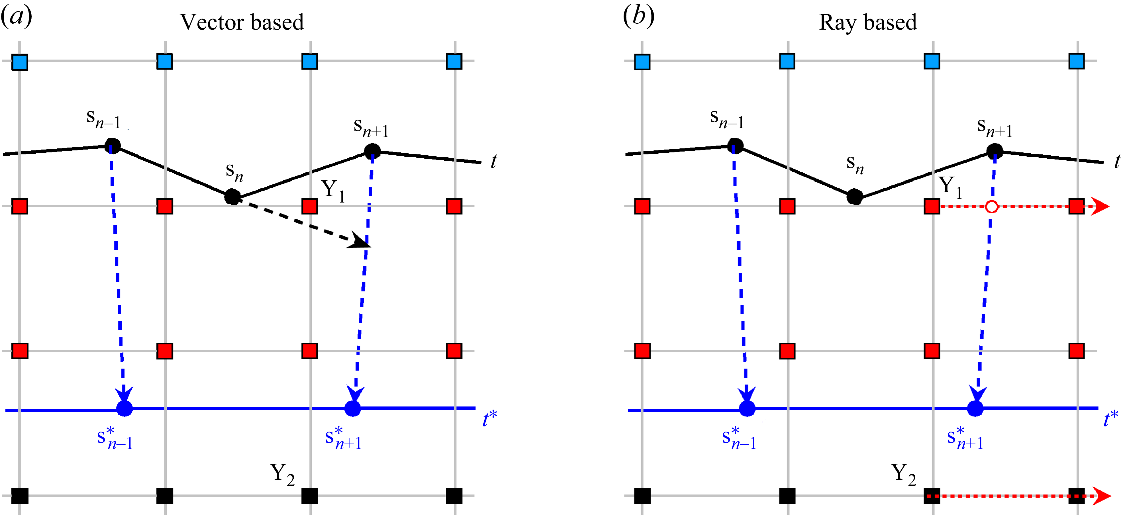


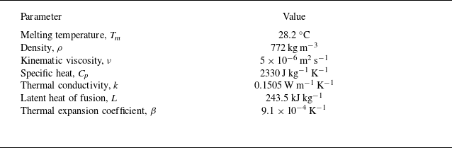


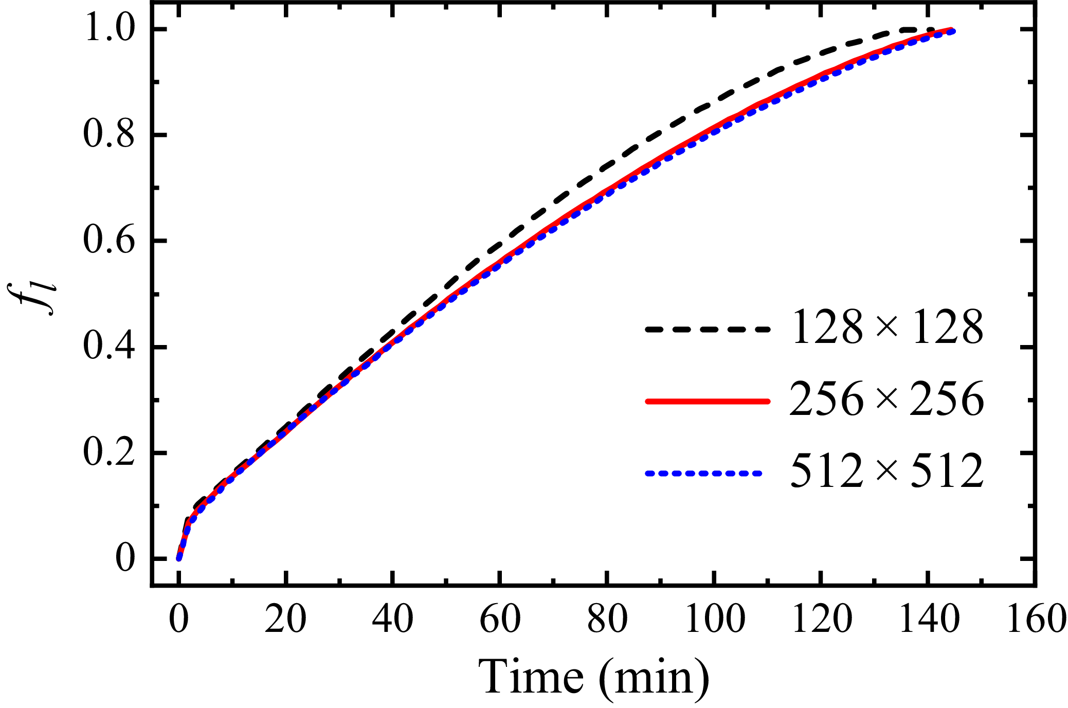


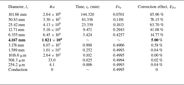


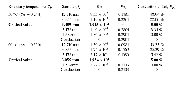


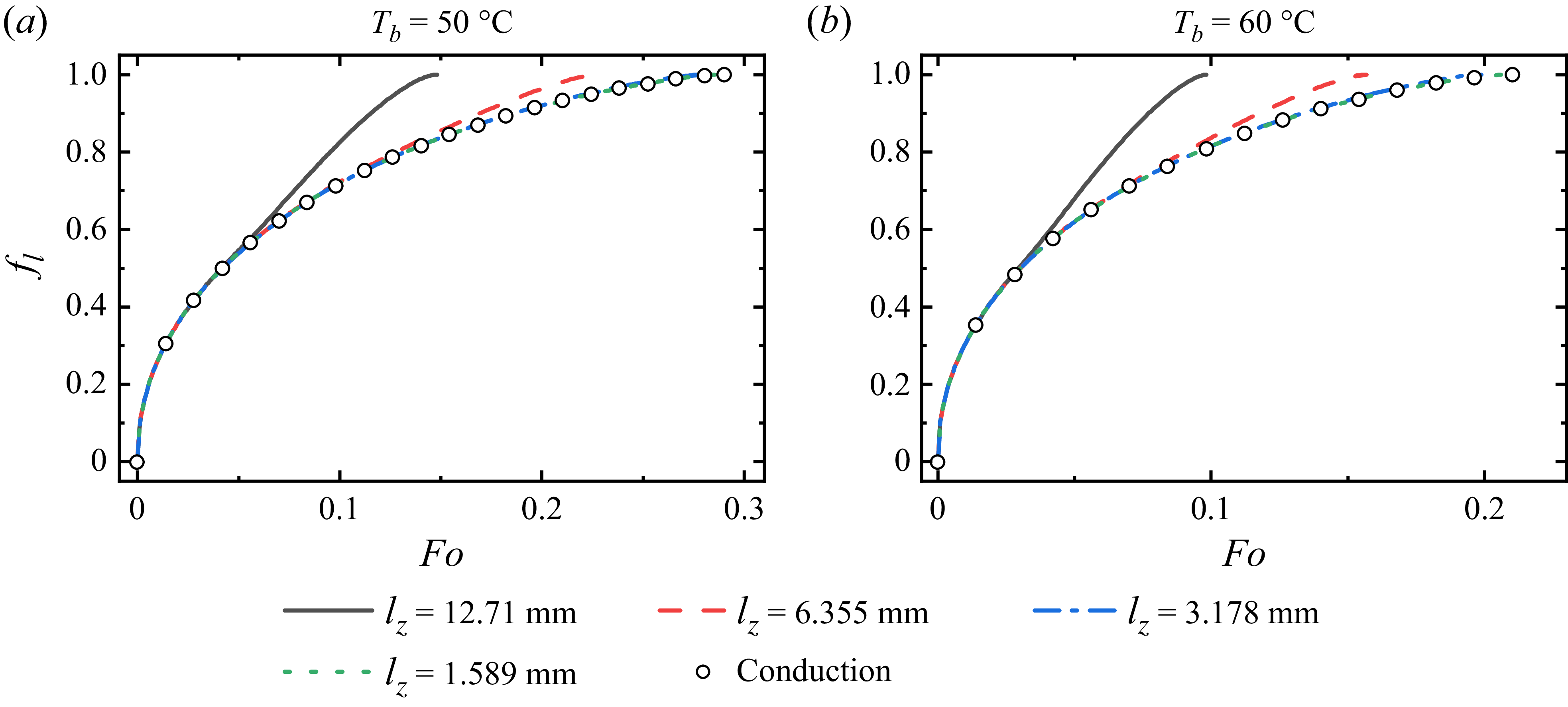


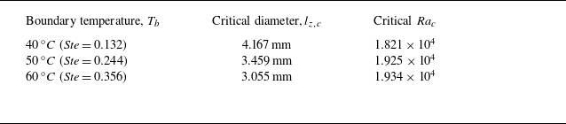


 Open access