





1. Introduction
During the night-time, surface radiative cooling leads to downslope (katabatic) flows that accumulate at the valley floor, forming a stably stratified layer, or cold pool, that persists throughout the night. After sunrise, surface heating initiates upslope (anabatic) flows, which gradually erode the cold pool and lead to the development of the convective boundary layer as the day progresses. This transition, known as the morning transition, plays a crucial role in phenomena such as pollutant transport, fog, and frost dissipation. However, numerical weather prediction models struggle to accurately capture this period due to the interplay of processes from both the convective and stable boundary layers (Angevine et al. Reference Angevine, Edwards, Lothon, LeMone and Osborne2020). This challenge is further exacerbated in valleys, where complex terrain introduces additional uncertainties due to inadequate parametrisations (Serafin et al. Reference Serafin2018; Farina et al. Reference Farina, Marchio, Barbano, di Sabatino and Zardi2023). Therefore, gaining a deeper understanding of the fundamental processes governing the morning transition in valleys is a critical first step towards improving their representation in numerical weather prediction models.
Numerous studies have examined large-scale idealised valley flow systems across a wide range of valley geometries using mesoscale numerical weather prediction models. Some have investigated valley–plain topographies, where the valley opens into a plain, leading to thermally driven along-valley circulations (Rampanelli, Zardi & Rotunno Reference Rampanelli, Zardi and Rotunno2004; Schmidli Reference Schmidli2013). Shapiro & Gomes (Reference Shapiro and Gomes2025) developed an analytical model for steady flow over a periodically repeating system of identical sloping valleys subjected to uniform heating or cooling. Their approach builds on the Prandtl model for slope flows, extending it to capture the flow dynamics within this periodic valley configuration. The model predicts symmetric flow patterns characterised by pairs of counter-rotating vortices on either side of each valley.
Others have focused exclusively on two-dimensional (2-D) valleys, analysing only cross-valley flow. Serafin & Zardi (Reference Serafin and Zardi2010) used large-eddy simulations to study daytime circulation in idealised valleys with both narrow and wide bases. Their findings highlight the interaction between thermal convection up the valley walls and compensating ‘top-down’ heating of the valley core due to subsidence. They also observed that while flow symmetry is largely maintained along the valley walls, asymmetric motions develop in the valley core. Similarly, Leukauf et al. (Reference Leukauf, Gohm, Rotach and Wagner2015) examined an idealised valley geometry with sinusoidal slopes and a narrow valley floor, focusing on how surface heating influences the break-up of initial stratification. They classified different flow regimes based on the strength of surface heat flux and the resulting stratification break-up. Additionally, Leukauf, Gohm & Rotach (Reference Leukauf, Gohm and Rotach2016) studied pollutant transport in a heated idealised valley, observing intrusions from the slopes into the stable core above the convective boundary layer. They also employed the dimensionless break-up parameter $B$
to quantify the combined effects of surface heating and initial stratification.
$B$
to quantify the combined effects of surface heating and initial stratification.
Several prior studies have further simplified the idealised valley geometry by considering a capped, triangular V-shaped valley. This approach facilitates a more detailed examination of small-scale dynamics, enabling researchers to extract precise flow field information through direct numerical simulations (DNS) or small-scale laboratory experiments. An example of this approach is the study by Princevac & Fernando (Reference Princevac and Fernando2008), which investigates the break-up of stratification in a V-shaped tank filled with initially stratified water. The experiment subjects the bottom walls to heating, allowing for a detailed analysis of how the stratification evolves under these conditions. They introduce the dimensionless break-up parameter $B$
to classify the break-up mechanisms as a function of both
$B$
to classify the break-up mechanisms as a function of both $B$
and the slope angle of the valley walls. A similar dimensionless break-up parameter was proposed by Leukauf et al. (Reference Leukauf, Gohm and Rotach2016), defined as the ratio of the energy required to break up an inversion to the cumulative surface sensible heat flux up to the time of break-up. This parameter facilitated the identification of similarity across simulations with varying stability conditions and forcing amplitudes.
$B$
and the slope angle of the valley walls. A similar dimensionless break-up parameter was proposed by Leukauf et al. (Reference Leukauf, Gohm and Rotach2016), defined as the ratio of the energy required to break up an inversion to the cumulative surface sensible heat flux up to the time of break-up. This parameter facilitated the identification of similarity across simulations with varying stability conditions and forcing amplitudes.
Most numerical studies on natural convection in triangular cavities have concentrated on attic-shaped geometries (Ridouane & Campo Reference Ridouane and Campo2006; Saha & Khan Reference Saha and Khan2011). In contrast, relatively few have investigated natural convection in valley-shaped geometries pertinent to the morning transition in valley flows, as exemplified by Princevac & Fernando (Reference Princevac and Fernando2008). Bhowmick et al. (Reference Bhowmick, Xu, Zhang and Saha2018) examined natural convection in a V-shaped cavity containing initially stratified water, following a set-up similar to that of Princevac & Fernando (Reference Princevac and Fernando2008). However, their numerical simulations were restricted to 2-D computations, and applied imposed temperature boundary conditions, rather than the flux conditions utilised in the experiments of Princevac & Fernando (Reference Princevac and Fernando2008). Consequently, the Rayleigh number served as the primary control parameter, complicating direct comparisons with the break-up parameter from the experiments. Other studies have explored natural convection in V-shaped cavities without considering stratification. Bhowmick et al. (Reference Bhowmick, Saha, Qiao and Xu2019, Reference Bhowmick, Xu, Molla and Saha2022) adopted 2-D computations with imposed temperature boundary conditions, and identified a series of bifurcations leading to chaotic flow, including pitchfork and Hopf bifurcations. A corresponding experimental study by Wang et al. (Reference Wang, Bhowmick, Tian, Saha and Xu2021) similarly observed the occurrence of a Hopf bifurcation. Cui, Xu & Saha (Reference Cui, Xu and Saha2015) considered natural convection in an attic-shaped triangular cavity heated from below and cooled from above, revealing complex 3-D flow structures such as longitudinal rolls. Their investigation adopted three-dimensional (3-D) computations.
Although previous studies have advanced our understanding of natural convection in triangular cavities – mostly through 2-D computations – a comprehensive grasp of 3-D flows in stably stratified idealised valleys remains incomplete. Moreover, conventional dimensionless parameters used to characterise these flows either do not sufficiently capture the full spectrum of flow regimes or have restricted applicability. To address these gaps, this research investigates the 3-D dynamics of stably stratified flows in idealised valleys heated from below. Building on the experimental study by Princevac & Fernando (Reference Princevac and Fernando2008), we adopt the same V-shaped valley geometry with a stably stratified ambient, and impose a constant heat flux condition on the valley walls to better replicate the conditions observed during the morning transition. Furthermore, our formulation aligns with Prandtl’s idealised representation of mountain and valley flows (Prandtl Reference Prandtl1952).
Beyond studies of natural convection in triangular cavities, our work also builds on previous research on the dynamics of stratified, convective flows in rectangular closed domains. For instance, Yalim, Welfert & Lopez (Reference Yalim, Welfert and Lopez2019) investigated the dynamics of a stably stratified fluid in a square cavity subjected to vertical oscillations, identifying the primary instabilities and the sequence of bifurcations that occur as the forcing parameter increases. Similarly, Grayer et al. (Reference Grayer, Yalim, Welfert and Lopez2020) examined the stability and dynamics of flow in a differentially heated square cavity with varying inclination angles. They classified the 2-D stability using the dimensionless buoyancy parameter $R_N$
, which quantifies the relative influence of buoyancy and viscous forces. Their study determined the critical
$R_N$
, which quantifies the relative influence of buoyancy and viscous forces. Their study determined the critical $R_N$
value at which steady flow persists, as well as the primary instabilities and limit cycles that emerge over a range of
$R_N$
value at which steady flow persists, as well as the primary instabilities and limit cycles that emerge over a range of $R_N$
and inclination angles. Extending this work to three dimensions, Shen, Hussam & Sheard (Reference Shen, Hussam and Sheard2025) investigated 3-D instabilities in the same differentially heated cavity, identifying the critical
$R_N$
and inclination angles. Extending this work to three dimensions, Shen, Hussam & Sheard (Reference Shen, Hussam and Sheard2025) investigated 3-D instabilities in the same differentially heated cavity, identifying the critical $R_N$
for 3-D instability, and characterising the structure of the dominant instability modes. Additionally, Jiang et al. (Reference Jiang, Zhao, Carmeliet, Nie and Xu2024) studied the full transition from laminar to chaotic flow above a circular heated surface with water as the working fluid, outlining the sequence of bifurcations and intermediate states, including periodic and puffing states, leading to chaotic flow.
$R_N$
for 3-D instability, and characterising the structure of the dominant instability modes. Additionally, Jiang et al. (Reference Jiang, Zhao, Carmeliet, Nie and Xu2024) studied the full transition from laminar to chaotic flow above a circular heated surface with water as the working fluid, outlining the sequence of bifurcations and intermediate states, including periodic and puffing states, leading to chaotic flow.
Recent studies on anabatic and katabatic Prandtl slope flows in infinitely wide domains have revealed new flow instabilities, including stationary longitudinal vortices and travelling transverse waves (Xiao & Senocak Reference Xiao and Senocak2019, Reference Xiao and Senocak2020). These investigations also introduced a new set of dimensionless parameters governing slope–flow stability, which are expected to be relevant for similar stratified slope–flow problems. Building on this foundation, our study extends Prandtl slope flows to valley flows, incorporating both the assumption of constant background stratification and the newly introduced dimensionless parameters. Additionally, Xiao & Senocak (Reference Xiao and Senocak2022) demonstrated that the combined effect of constant ambient stratification and surface cooling distinctly alters turbulent open channel flow dynamics compared to stratification driven solely by surface cooling. This further reinforces our decision to assume a constant background stratification in the valley geometry.
In our previous investigation of flows in V-shaped valleys (Stofanak, Xiao & Senocak Reference Stofanak, Xiao and Senocak2024), we used linear stability analysis (LSA) and 3-D DNS to characterise the 2-D flow states in the valley. This analysis revealed a distinctive bifurcation diagram, featuring a perfect pitchfork bifurcation that gives rise to two asymmetric states, as well as an unusual bifurcation leading to unstable upslope and downslope symmetric states. Additionally, we identified a unique self-organising 3-D instability that ultimately returns to a steady 2-D state in the long-time limit (Stofanak, Xiao & Senocak Reference Stofanak, Xiao and Senocak2025). In this study, we extend our analysis to investigate 3-D states using both LSA and DNS, providing a comprehensive characterisation of the transition from the quiescent pure-conduction state to the fully 3-D chaotic state. Additionally, we delineate the flow regimes associated with each state based on a newly introduced dimensionless parameter, gaining key insights into the flow dynamics.
2. Problem description and methods
2.1. Problem description
We consider a V-shaped cavity filled with a stably stratified fluid and heated from below, serving as an idealised model of valley flows. A schematic of the 3-D geometry is shown in figure 1 with key parameters, including the height of the valley $H$
, the slope angle of the valley walls relative to horizontal
$H$
, the slope angle of the valley walls relative to horizontal $\alpha$
, and the length in the
$\alpha$
, and the length in the $z$
direction
$z$
direction $L_z$
. The V-shaped valley lies in the
$L_z$
. The V-shaped valley lies in the $x$
–
$x$
– $y$
plane with horizontal velocity
$y$
plane with horizontal velocity $u$
and vertical velocity
$u$
and vertical velocity $v$
, and the geometry is homogeneous along the
$v$
, and the geometry is homogeneous along the $z$
direction with spanwise velocity
$z$
direction with spanwise velocity $w$
. In our previous studies, we used LSA and Navier–Stokes simulations to investigate the 2-D states (Stofanak et al. Reference Stofanak, Xiao and Senocak2024) and the primary 3-D instability at low parameter values (Stofanak et al. Reference Stofanak, Xiao and Senocak2025). Here, we use the same combination of LSA and Navier–Stokes simulations to investigate 3-D states in the valley and the dependence on the dimensionless parameter space. For all simulations, a minimum
$w$
. In our previous studies, we used LSA and Navier–Stokes simulations to investigate the 2-D states (Stofanak et al. Reference Stofanak, Xiao and Senocak2024) and the primary 3-D instability at low parameter values (Stofanak et al. Reference Stofanak, Xiao and Senocak2025). Here, we use the same combination of LSA and Navier–Stokes simulations to investigate 3-D states in the valley and the dependence on the dimensionless parameter space. For all simulations, a minimum $L_z$
of twice the height is used, with
$L_z$
of twice the height is used, with $L_z$
extending up to 16 times the height for some simulations.
$L_z$
extending up to 16 times the height for some simulations.
Schematic of the 3-D valley geometry. The valley is filled with a stably stratified fluid characterised by the Brunt–Väisälä frequency $N$
, with key parameters and coordinate axes indicated. The 2-D cross-section lies in the
$N$
, with key parameters and coordinate axes indicated. The 2-D cross-section lies in the $x$
–
$x$
– $y$
plane, with the
$y$
plane, with the $z$
axis directed out of the page. All visualisations in this work adopt the same coordinate system and origin.
$z$
axis directed out of the page. All visualisations in this work adopt the same coordinate system and origin.

We define buoyancy as the scaled perturbation potential temperature $\varTheta$
with
$\varTheta$
with $b = g ( \varTheta - \varTheta _e ) / \varTheta _r$
, where
$b = g ( \varTheta - \varTheta _e ) / \varTheta _r$
, where $\varTheta _e$
is the background or environmental potential temperature that varies in the direction of gravity only, and
$\varTheta _e$
is the background or environmental potential temperature that varies in the direction of gravity only, and $\varTheta _r$
is a reference potential temperature. Following the Prandtl model for slope flows (Prandtl Reference Prandtl1952), a constant background stratification is given by the buoyancy frequency, or Brunt–Väisälä frequency, defined as
$\varTheta _r$
is a reference potential temperature. Following the Prandtl model for slope flows (Prandtl Reference Prandtl1952), a constant background stratification is given by the buoyancy frequency, or Brunt–Väisälä frequency, defined as $N = \sqrt { (g / \varTheta _r )\, {\rm d} \varTheta _e / {\rm d} y}$
. Therefore, the buoyancy represents a perturbation from an assumed constant, stable background state. This is relevant to the scenario of an isolated valley early in the morning transition when a strong inversion still exists (Whiteman Reference Whiteman2000). The buoyancy boundary conditions are shown in figure 1, with a constant positive buoyancy flux representing surface heating applied on both bottom walls defined as
$N = \sqrt { (g / \varTheta _r )\, {\rm d} \varTheta _e / {\rm d} y}$
. Therefore, the buoyancy represents a perturbation from an assumed constant, stable background state. This is relevant to the scenario of an isolated valley early in the morning transition when a strong inversion still exists (Whiteman Reference Whiteman2000). The buoyancy boundary conditions are shown in figure 1, with a constant positive buoyancy flux representing surface heating applied on both bottom walls defined as $B_s = \beta\partial b/ \partial n$
, where
$B_s = \beta\partial b/ \partial n$
, where $\beta$
is the thermal diffusivity, and
$\beta$
is the thermal diffusivity, and $n$
is the direction normal to the sloping boundaries. A constant
$n$
is the direction normal to the sloping boundaries. A constant $b = 0$
is imposed on the top boundary. For velocity, no-slip conditions are imposed on the bottom walls, and a free-slip (stress-free) condition is imposed on the top boundary.
$b = 0$
is imposed on the top boundary. For velocity, no-slip conditions are imposed on the bottom walls, and a free-slip (stress-free) condition is imposed on the top boundary.
Our choice of boundary conditions and the symmetric configuration is motivated by the laboratory-scale experimental study of Princevac & Fernando (Reference Princevac and Fernando2008), which employed a density-stratified saline solution in a V-shaped tank. We acknowledge that the idealisations adopted here – such as constant surface heat flux, uniform ambient stratification, and stress-free conditions at the domain top – do not capture the full complexity and heterogeneity of real valley flows. Nevertheless, these simplifications are grounded in the theoretical modelling exemplified by Prandtl’s classical slope–flow model (Prandtl Reference Prandtl1952), which has proven remarkably successful in reproducing key structural features of katabatic winds observed in mountainous terrain (Papadopoulos et al. Reference Papadopoulos, Helmis, Soilemes, Kalogiros, Papageorgas and Asimakopoulos1997).
The governing equations are given by the Navier–Stokes equations with the Oberbeck–Boussinesq approximation, written as
 \begin{align} \boldsymbol{\nabla }\boldsymbol{\cdot }\boldsymbol{u} &= 0,\end{align}
 \begin{align} \frac {\partial \boldsymbol{u}}{\partial t} + \boldsymbol{u} \boldsymbol{\cdot }\boldsymbol{\nabla }\boldsymbol{u} &= - \boldsymbol{\nabla }p + \nu\, {\nabla} ^2 \boldsymbol{u} + b \boldsymbol{e}_y,\end{align}
 \begin{align} \frac {\partial b}{\partial t} + \boldsymbol{u} \boldsymbol{\cdot }\boldsymbol{\nabla }b &= \beta\,{\nabla} ^2 b - N^2 \boldsymbol{u} \boldsymbol{\cdot }\boldsymbol{e}_y,\end{align}
where $p$
is the specific pressure,
$p$
is the specific pressure, $\nu$
is the kinematic viscosity,
$\nu$
is the kinematic viscosity, $\beta$
is the thermal diffusivity, and
$\beta$
is the thermal diffusivity, and $\boldsymbol{e}_y$
is the unit vector in the
$\boldsymbol{e}_y$
is the unit vector in the $y$
direction, representing the direction of the gravity vector. Additionally, we note that the last term in (2.3) is due to the assumption of the constant background stratification, consistent with the Prandtl model (Prandtl Reference Prandtl1952).
$y$
direction, representing the direction of the gravity vector. Additionally, we note that the last term in (2.3) is due to the assumption of the constant background stratification, consistent with the Prandtl model (Prandtl Reference Prandtl1952).
For the valley geometry presented in figure 1, the governing equations admit six external parameters: $B_s, N, \nu , \beta , H, \alpha$
. Application of the Buckingham-
$B_s, N, \nu , \beta , H, \alpha$
. Application of the Buckingham- $\pi$
theorem yields the dimensionless parameters
$\pi$
theorem yields the dimensionless parameters
 \begin{align} \varPi _s = \frac {B_s}{\beta N^2}, \quad \varPi _h = \frac {{\textit{NH}}^2}{\beta }, \quad \textit{Pr} = \frac {\nu }{\beta }, \quad \alpha , \end{align}
where ${\textit{Pr}}$
is the Prandtl number, and
${\textit{Pr}}$
is the Prandtl number, and $\alpha$
is the slope angle of the valley walls. The stratification perturbation parameter
$\alpha$
is the slope angle of the valley walls. The stratification perturbation parameter $\varPi _s$
represents the ratio of the surface buoyancy flux to the background stable stratification (Xiao & Senocak Reference Xiao and Senocak2019). The height parameter
$\varPi _s$
represents the ratio of the surface buoyancy flux to the background stable stratification (Xiao & Senocak Reference Xiao and Senocak2019). The height parameter $\varPi _h$
represents the ratio between the thermal diffusion and stratification time scales (Stofanak et al. Reference Stofanak, Xiao and Senocak2024). This set of dimensionless parameters is agnostic to boundary conditions on the valley top. As shown in § 2.3, for the given boundary conditions on the valley walls and top, we are able to reduce this set from four to three parameters.
$\varPi _h$
represents the ratio between the thermal diffusion and stratification time scales (Stofanak et al. Reference Stofanak, Xiao and Senocak2024). This set of dimensionless parameters is agnostic to boundary conditions on the valley top. As shown in § 2.3, for the given boundary conditions on the valley walls and top, we are able to reduce this set from four to three parameters.
2.2. The LSA
To perform LSA, we linearise the Navier–Stokes equations around an arbitrary 3-D base flow given by $U(x,y,z), V(x,y,z), W(x,y,z), P(x,y,z), B(x,y,z)$
. We then assume that a small disturbance
$U(x,y,z), V(x,y,z), W(x,y,z), P(x,y,z), B(x,y,z)$
. We then assume that a small disturbance $\boldsymbol{q}$
is added to this base flow, of the form
$\boldsymbol{q}$
is added to this base flow, of the form
 \begin{align} \boldsymbol{q}(x, y, z, t) = \hat{\boldsymbol{q}} \exp \left (\omega t \right ), \end{align}
where $\hat{\boldsymbol{q}} = [\hat {u}(x,y,z), \hat {v}(x,y,z), \hat {w}(x,y,z), \hat {p}(x,y,z), \hat {b}(x,y,z) ]$
represents the 3-D disturbance quantities. Substituting this expression for the disturbances into the linearised Navier–Stokes equations gives a set of equations for the disturbance quantities, and
$\hat{\boldsymbol{q}} = [\hat {u}(x,y,z), \hat {v}(x,y,z), \hat {w}(x,y,z), \hat {p}(x,y,z), \hat {b}(x,y,z) ]$
represents the 3-D disturbance quantities. Substituting this expression for the disturbances into the linearised Navier–Stokes equations gives a set of equations for the disturbance quantities, and $\omega$
dependent on the base flow. These equations can be written as a generalised eigenvalue problem of the form
$\omega$
dependent on the base flow. These equations can be written as a generalised eigenvalue problem of the form
 \begin{align} \boldsymbol{A} \hat{\boldsymbol{q}}(x,y,z) = \omega \boldsymbol{B} \hat{\boldsymbol{q}}(x,y,z), \end{align}
where $\omega$
is the eigenvalue, and the disturbance quantities
$\omega$
is the eigenvalue, and the disturbance quantities $\hat{\boldsymbol{q}}$
are the eigenvectors. Solving this eigenvalue problem represent a global stability analysis in which the base flow and disturbance quantities depends on all three spatial dimensions. In this paper, we perform bi-global stability analysis in which the base flow and disturbance quantities depend on only two spatial dimensions, and are assumed periodic in the third. In the case of bi-global stability analysis, the disturbance is of the form
$\hat{\boldsymbol{q}}$
are the eigenvectors. Solving this eigenvalue problem represent a global stability analysis in which the base flow and disturbance quantities depends on all three spatial dimensions. In this paper, we perform bi-global stability analysis in which the base flow and disturbance quantities depend on only two spatial dimensions, and are assumed periodic in the third. In the case of bi-global stability analysis, the disturbance is of the form $\boldsymbol{q}(x, y, z, t) = \hat{\boldsymbol{q}}(x,y) \exp ({\rm i}k_z z + \omega t )$
, where
$\boldsymbol{q}(x, y, z, t) = \hat{\boldsymbol{q}}(x,y) \exp ({\rm i}k_z z + \omega t )$
, where $k_z$
is the wavenumber in the homogeneous
$k_z$
is the wavenumber in the homogeneous $z$
direction, and the solution to the eigenvalue problem further depends on the choice of wavenumber.
$z$
direction, and the solution to the eigenvalue problem further depends on the choice of wavenumber.
In our investigation of all possible flow states in a V-shaped valley heated from the sides, we start from the most basic state, which we call the pure-conduction state, or the zero flow state. Given the boundary conditions for buoyancy at valley walls and top, this state can be determined from the Navier–Stokes equations assuming that all velocity components are zero. This gives an exact solution for the buoyancy and pressure as
 \begin{align} B(y) = \frac {B_s}{\beta \cos \alpha } \left ( H - y \right ), \quad P(y) = \frac {- B_s}{2 \beta \cos \alpha } \left ( y - H \right )^2, \end{align}
where $B_s$
is the imposed surface buoyancy flux. This exact solution is used as the base state as the starting point of our LSA. Substitution of this base state as well as the assumption of periodicity in the third direction into the LSA equations leads to a simplified set of equations given by
$B_s$
is the imposed surface buoyancy flux. This exact solution is used as the base state as the starting point of our LSA. Substitution of this base state as well as the assumption of periodicity in the third direction into the LSA equations leads to a simplified set of equations given by
 \begin{align} \frac {\partial \hat {u}}{\partial x} + \frac {\partial \hat {v}}{\partial y} + {\rm i}k_z \hat {w} &= 0,\end{align}
 \begin{align} \omega \hat {u} & = - \frac {\partial \hat {p}}{\partial x} + \nu \left ( \frac {\partial ^2\hat {u}}{\partial x^2}+\frac {\partial ^2\hat {u}}{\partial y^2} - k_{z}^{2} \hat {u} \right ),\end{align}
 \begin{align} \omega \hat {v} & = - \frac {\partial \hat {p}}{\partial y} + \nu \left ( \frac {\partial ^2\hat {v}}{\partial x^2}+\frac {\partial ^2\hat {v}}{\partial y^2} - k_{z}^{2} \hat {v} \right ) + \hat {b} ,\end{align}
 \begin{align} \omega \hat {w} & = -{\rm i}k_z \hat {p} + \nu \left ( \frac {\partial ^2\hat {w}}{\partial x^2}+\frac {\partial ^2\hat {w}}{\partial y^2} - k_{z}^{2} \hat {w} \right )\! ,\end{align}
 \begin{align} \omega \hat {b} & = \beta \left ( \frac {\partial ^2\hat {b}}{\partial x^2}+\frac {\partial ^2\hat {b}}{\partial y^2} - k_{z}^{2} \hat {b} \right ) + \left ( \frac {B_s}{\beta \cos \alpha } - N^2 \right ) \hat {v}.\end{align}
From these linearised equations, it is clear that for the same slope angle, kinematic viscosity and thermal diffusivity, the system of equations depends only on the value of $ (B_s/\beta \cos \alpha ) - N^2$
. The first term in this difference,
$ (B_s/\beta \cos \alpha ) - N^2$
. The first term in this difference, $B_s/\beta \cos \alpha$
, represents the unstable vertical buoyancy gradient due to the heating of the bottom walls, whereas
$B_s/\beta \cos \alpha$
, represents the unstable vertical buoyancy gradient due to the heating of the bottom walls, whereas $N^2$
represents the imposed stable background buoyancy gradient. Therefore, this term represents the composite vertical buoyancy gradient between the combined effects of the surface heating and the background stratification.
$N^2$
represents the imposed stable background buoyancy gradient. Therefore, this term represents the composite vertical buoyancy gradient between the combined effects of the surface heating and the background stratification.
Because of this, we can define the following scales based on this composite value to normalise all dimensional quantities:
 \begin{align} \begin{aligned} l_0 &= H, \quad u_0 = H \sqrt {G_y - N^2}, \quad b_0 = H \left(G_y - N^2\right), \\ p_0 &= H^2 \left(G_y - N^2\right)\! , \quad t_{{0,c}} = \frac {1}{\sqrt {G_y - N^2}}, \end{aligned} \end{align}
where $G_y = B_s/ \beta \cos \alpha$
. The convective time scale
$G_y = B_s/ \beta \cos \alpha$
. The convective time scale $t_{{0,c}}$
is defined as the ratio of the characteristic length scale to the characteristic velocity scale, i.e.
$t_{{0,c}}$
is defined as the ratio of the characteristic length scale to the characteristic velocity scale, i.e. $t_{{0,c}}=l_0 / u_0$
. Alternatively, a diffusion time scale can be defined as
$t_{{0,c}}=l_0 / u_0$
. Alternatively, a diffusion time scale can be defined as $t_{0,d} = H^2/\beta$
, and a buoyancy time scale can be defined as
$t_{0,d} = H^2/\beta$
, and a buoyancy time scale can be defined as $t_{{0,b}} = 1/N$
, but here we use the convective time scale
$t_{{0,b}} = 1/N$
, but here we use the convective time scale $t_{{0,c}}$
to non-dimensionalise the equations and results below. However, because the diffusion time scale
$t_{{0,c}}$
to non-dimensionalise the equations and results below. However, because the diffusion time scale $t_{{0,d}}$
is much longer than both other time scales, with
$t_{{0,d}}$
is much longer than both other time scales, with $O(t_{{0, c}})\sim 1$
,
$O(t_{{0, c}})\sim 1$
, $O(t_{{0, b}})\sim 1$
and
$O(t_{{0, b}})\sim 1$
and $O(t_{{0, d}})\sim 1000$
, the diffusion time scale is used as a guide to determine the periods for which to run simulations in order to come to a steady or statistically steady state.
$O(t_{{0, d}})\sim 1000$
, the diffusion time scale is used as a guide to determine the periods for which to run simulations in order to come to a steady or statistically steady state.
Using the defined scales, we non-dimensionalise the linearised equations for the pure-conduction base state, (2.8)–(2.12), to the following:
 \begin{align} \frac {\partial \hat {u}_n}{\partial x_n} + \frac {\partial \hat {v}_n}{\partial y_n} + {\rm i}k_z \hat {w}_n &= 0,\end{align}
 \begin{align} \omega _n \hat {u}_n & = - \frac {\partial \hat {p}_n}{\partial x_n} + \frac {\textit{Pr}}{\varPi _c} \left ( \frac {\partial ^2\hat {u}_n}{\partial x_n^2}+\frac {\partial ^2\hat {u}_n}{\partial y_n^2} - k_{z}^{2} \hat {u}_n \right ),\end{align}
 \begin{align} \omega _n \hat {v}_n & = - \frac {\partial \hat {p}_n}{\partial y_n} + \frac {\textit{Pr}}{\varPi _c} \left ( \frac {\partial ^2\hat {v}_n}{\partial x_n^2}+\frac {\partial ^2\hat {v}_n}{\partial y_n^2} - k_{z}^{2} \hat {v}_n \right ) + \hat {b}_n ,\end{align}
 \begin{align} \omega _n \hat {w}_n & = -{\rm i}k_z \hat {p}_n + \frac {\textit{Pr}}{\varPi _c} \left ( \frac {\partial ^2\hat {w}_n}{\partial x_n^2}+\frac {\partial ^2\hat {w}_n}{\partial y_n^2} - k_{z}^{2} \hat {w}_n \right )\! ,\end{align}
 \begin{align} \omega _n \hat {b}_n & = \frac {1}{\varPi _c} \left ( \frac {\partial ^2\hat {b}_n}{\partial x_n^2}+\frac {\partial ^2\hat {b}_n}{\partial y_n^2} - k_{z}^{2} \hat {b}_n \right ) + \hat {v}_n,\end{align}
where the subscript $n$
denotes a non-dimensional variable, such as
$n$
denotes a non-dimensional variable, such as $u_n = u/u_0$
, and we define a new, composite dimensionless parameter
$u_n = u/u_0$
, and we define a new, composite dimensionless parameter $\varPi _c$
as
$\varPi _c$
as
 \begin{align} \varPi _c = \frac {H^2 \sqrt {G_y - N^2}}{\beta }. \end{align}
Based on the linearised equations, and assuming a constant slope angle, the solution to the eigenvalue problem depends on only two dimensionless parameters, the Prandtl number ${\textit{Pr}}$
, and the newly introduced
${\textit{Pr}}$
, and the newly introduced $\varPi _c$
, which we refer to as the composite stratification parameter.
$\varPi _c$
, which we refer to as the composite stratification parameter.
2.3. Dimensionless form of the nonlinear equations
Following the same approach used for the linearised equations, we decompose the buoyancy and pressure field into the pure-conduction base state plus some finite-amplitude perturbation
 \begin{align} b(x,y,z,t) = B(y) + b^{\prime }(x,y,z,t), \end{align}
 \begin{align} p(x,y,z,t) = P(y) + p^{\prime }(x,y,z,t), \end{align}
and non-dimensionalise the nonlinear equations by the composite scales defined in (2.13), to obtain
 \begin{align} \frac {\partial \boldsymbol{u}_n}{\partial t_n} + \boldsymbol{u}_n \boldsymbol{\cdot }\boldsymbol{\nabla }\boldsymbol{u}_n &= - \boldsymbol{\nabla }p_{n}^{\prime } + \frac {\textit{Pr}}{\varPi _c} {\nabla} ^2 \boldsymbol{u}_n + b_{n}^{\prime } \boldsymbol{e}_y, \end{align}
 \begin{align} \frac {\partial b_{n}^{\prime }}{\partial t_n} + \boldsymbol{u}_n \boldsymbol{\cdot }\boldsymbol{\nabla }b_{n}^{\prime } &= \frac {1}{\varPi _c} {\nabla} ^2 b_{n}^{\prime } + \boldsymbol{u}_n \boldsymbol{\cdot }\boldsymbol{e}_y. \end{align}
Similar to the linearised equations, for fixed slope angle and Prandtl number, the nonlinear equations depend on a single dimensionless parameter $\varPi _c$
.
$\varPi _c$
.
Equations (2.22) and (2.23) take this special form owing to the specific combination of boundary conditions on valley walls and top, which permits the exact pure-conduction solution (2.7). Neumann-type constant buoyancy flux on valley walls and Dirichlet-type constant buoyancy at the valley top define a zero-flow base state with linear-with-height profiles for buoyancy and pressure; combining this base state with the background stratification yields a composite stratification. Other boundary conditions – such as constant buoyancy at valley walls or buoyancy flux at the valley top – would produce a base state that is no longer a simple linear-with-height profile, precluding this simplification. In Appendix A, we present the dimensionless nonlinear equations for boundary conditions that do not permit the decomposition in (2.20)–(2.21), in which case an additional dimensionless parameter $\varPi _h = N H^2 \beta ^{-1}$
depending on valley height arises.
$\varPi _h = N H^2 \beta ^{-1}$
depending on valley height arises.
The composite stratification parameter $\varPi _c$
can be interpreted as the product of an internal Reynolds number and Prandtl number. Specifically, if a Reynolds number for the flow is defined through the internal scales as
$\varPi _c$
can be interpreted as the product of an internal Reynolds number and Prandtl number. Specifically, if a Reynolds number for the flow is defined through the internal scales as $Re = u_0 l_0 / \nu$
, then the composite stratification parameter can be viewed as
$Re = u_0 l_0 / \nu$
, then the composite stratification parameter can be viewed as $\varPi _c = Re\, Pr$
, which is the Péclet number based on the internal flow scales. The advantage of using
$\varPi _c = Re\, Pr$
, which is the Péclet number based on the internal flow scales. The advantage of using $\varPi _c$
is that it can be defined a priori based on external control parameters.
$\varPi _c$
is that it can be defined a priori based on external control parameters.
Although the slope angle $\alpha$
does not explicitly appear in the linearised or nonlinear equations, its direct influence arises through the boundary conditions. This dependence is due to its effect on both the angle itself and the effective surface area for heating. Specifically, at the bottom walls, the boundary condition is given as a heat flux normal to the wall, meaning that
$\alpha$
does not explicitly appear in the linearised or nonlinear equations, its direct influence arises through the boundary conditions. This dependence is due to its effect on both the angle itself and the effective surface area for heating. Specifically, at the bottom walls, the boundary condition is given as a heat flux normal to the wall, meaning that $\partial b/\partial n$
is fixed, where the normal direction is defined in terms of slope angle as the unit vector
$\partial b/\partial n$
is fixed, where the normal direction is defined in terms of slope angle as the unit vector $\boldsymbol{n} = ( \pm \sin \alpha , \cos \alpha )$
, with the sign positive for the left-hand slope and negative for the right-hand slope.
$\boldsymbol{n} = ( \pm \sin \alpha , \cos \alpha )$
, with the sign positive for the left-hand slope and negative for the right-hand slope.
2.4. Numerical methods
We use the open-source, spectral/hp element code Nektar $++$
(Cantwell et al. Reference Cantwell2015; Moxey et al. Reference Moxey2020), with a finite element discretisation of 31 elements along each bottom wall of the valley, and polynomial order four. A Fourier expansion method is used in the third direction, with 16 Fourier modes per non-dimensional length. A finer mesh was used for the highest
$++$
(Cantwell et al. Reference Cantwell2015; Moxey et al. Reference Moxey2020), with a finite element discretisation of 31 elements along each bottom wall of the valley, and polynomial order four. A Fourier expansion method is used in the third direction, with 16 Fourier modes per non-dimensional length. A finer mesh was used for the highest $\varPi _c$
cases reported in this paper, with the finest mesh using 41 elements along each bottom wall, polynomial order four, and 32 Fourier modes per non-dimensional length in the homogeneous direction. The eigenvalue problem of the LSA is solved using the modified Arnoldi method included in Nektar
$\varPi _c$
cases reported in this paper, with the finest mesh using 41 elements along each bottom wall, polynomial order four, and 32 Fourier modes per non-dimensional length in the homogeneous direction. The eigenvalue problem of the LSA is solved using the modified Arnoldi method included in Nektar $++$
, with a typical Krylov subspace of between 32 and 512, converging to a residual of less than
$++$
, with a typical Krylov subspace of between 32 and 512, converging to a residual of less than $10^{-6}$
. Our LSA and DNS results are validated by comparison to prior published results for Prandtl slope flow. Specifically, we perform LSA and DNS of Prandtl slope flow, and obtain the same results as described in Xiao & Senocak (Reference Xiao and Senocak2020), which used a separate in-house code. For our valley geometry, we show the mesh independence for a case of intermediate parameter values in table 1, which shows the total kinetic energy of the steady state, and velocity
$10^{-6}$
. Our LSA and DNS results are validated by comparison to prior published results for Prandtl slope flow. Specifically, we perform LSA and DNS of Prandtl slope flow, and obtain the same results as described in Xiao & Senocak (Reference Xiao and Senocak2020), which used a separate in-house code. For our valley geometry, we show the mesh independence for a case of intermediate parameter values in table 1, which shows the total kinetic energy of the steady state, and velocity $u$
at a point as a function of increasing mesh resolution. Additionally, more details of validation of our numerical solver are provided in our previously published results (Stofanak et al. Reference Stofanak, Xiao and Senocak2024, Reference Stofanak, Xiao and Senocak2025).
$u$
at a point as a function of increasing mesh resolution. Additionally, more details of validation of our numerical solver are provided in our previously published results (Stofanak et al. Reference Stofanak, Xiao and Senocak2024, Reference Stofanak, Xiao and Senocak2025).
Total kinetic energy and $u$
velocity at point
$u$
velocity at point $(0, 0.9, 0)$
of 2-D asymmetric steady state flow at
$(0, 0.9, 0)$
of 2-D asymmetric steady state flow at $\varPi _c = 297$
for increasing mesh resolution. Velocity is normalised by
$\varPi _c = 297$
for increasing mesh resolution. Velocity is normalised by $u_0=0.2122$
, and kinetic energy is normalised by
$u_0=0.2122$
, and kinetic energy is normalised by $u_{0}^{2}$
.
$u_{0}^{2}$
.

3. Results
We now present results of the primary instabilities and flow states observed in the heated valley geometry for increasing $\varPi _c$
. All results are shown in non-dimensional form using the scales in (2.13), unless otherwise noted.
$\varPi _c$
. All results are shown in non-dimensional form using the scales in (2.13), unless otherwise noted.
3.1.
Classification of flow states for increasing $\varPi _c$

3.1.1. Pure-conduction state
We begin with LSA to identify the primary instabilities, before proceeding to determine the corresponding steady states. As stated in § 2, we apply our LSA to a quiescent base state that represents pure conduction, characterised by a linear buoyancy profile, a quadratic pressure distribution, and a zero velocity field. In our previous work (Stofanak et al. Reference Stofanak, Xiao and Senocak2024), we considered a fixed $\varPi _h = 1500$
and determined the critical value for instability based on
$\varPi _h = 1500$
and determined the critical value for instability based on $\varPi _s$
. However, our analysis in § 2.3 shows that the equations with the pure-conduction base flow depend only on
$\varPi _s$
. However, our analysis in § 2.3 shows that the equations with the pure-conduction base flow depend only on $\varPi _c$
, allowing us to determine a critical value at which the base state becomes unstable for any combination of
$\varPi _c$
, allowing us to determine a critical value at which the base state becomes unstable for any combination of $\varPi _s$
and
$\varPi _s$
and $\varPi _h$
, at fixed Prandtl number. We compute
$\varPi _h$
, at fixed Prandtl number. We compute $\varPi _c$
as
$\varPi _c$
as
 \begin{align} \varPi _c = \varPi _h \sqrt {\frac {\varPi _s}{\cos \alpha } - 1}. \end{align}
In Stofanak et al. (Reference Stofanak, Xiao and Senocak2024), we showed that the pure-conduction state becomes unstable at critical value approximately $\varPi _s = 0.8751$
at
$\varPi _s = 0.8751$
at $\varPi _h = 1500$
. Therefore, the corresponding critical value of
$\varPi _h = 1500$
. Therefore, the corresponding critical value of $\varPi _c$
is 153.5. Below this value, the pure-conduction state is linearly stable.
$\varPi _c$
is 153.5. Below this value, the pure-conduction state is linearly stable.
A distinctive feature of $\varPi _c$
in (3.1) is that it takes imaginary values below the critical instability threshold. This arises when the stable background stratification
$\varPi _c$
in (3.1) is that it takes imaginary values below the critical instability threshold. This arises when the stable background stratification $N^2$
exceeds the unstable vertical buoyancy gradient
$N^2$
exceeds the unstable vertical buoyancy gradient $G_y$
induced by surface heating, which fails to overcome the stabilising stratification, leaving only the quiescent state. From the definition of
$G_y$
induced by surface heating, which fails to overcome the stabilising stratification, leaving only the quiescent state. From the definition of $\varPi _c$
in terms of
$\varPi _c$
in terms of $\varPi _h$
and
$\varPi _h$
and $\varPi _s$
, the following necessary condition for convective motion is derived:
$\varPi _s$
, the following necessary condition for convective motion is derived:
 \begin{align} \varPi _s \gt \cos \alpha . \end{align}
When this condition is not met, the radicand in (3.1) is negative, and $\varPi _c$
becomes imaginary. Therefore, for any slope angle
$\varPi _c$
becomes imaginary. Therefore, for any slope angle $\alpha$
, a minimum
$\alpha$
, a minimum $\varPi _s$
must be exceeded to initiate instability, regardless of
$\varPi _s$
must be exceeded to initiate instability, regardless of $\varPi _h$
. For example, at
$\varPi _h$
. For example, at $\alpha = 30^{\circ }$
, the critical value is
$\alpha = 30^{\circ }$
, the critical value is $\varPi _s = 0.8751 \gt \cos \alpha$
. The LSA and DNS at
$\varPi _s = 0.8751 \gt \cos \alpha$
. The LSA and DNS at $\alpha = 10^{\circ }$
confirm this, where the critical
$\alpha = 10^{\circ }$
confirm this, where the critical $\varPi _s$
must exceed 0.985. This reveals that the critical
$\varPi _s$
must exceed 0.985. This reveals that the critical $\varPi _s$
for instability increases with decreasing slope angle.
$\varPi _s$
for instability increases with decreasing slope angle.
3.1.2. Self-organising 2-D flow state
Above $\varPi _c = 153.5$
, two distinct 2-D instabilities emerge: one representing a 2-D asymmetric state, and the other representing a 2-D symmetric state. The steady-state solutions for the asymmetric and symmetric states are shown in figure 2 for
$\varPi _c = 153.5$
, two distinct 2-D instabilities emerge: one representing a 2-D asymmetric state, and the other representing a 2-D symmetric state. The steady-state solutions for the asymmetric and symmetric states are shown in figure 2 for $\varPi _c = 297$
. Secondary LSA of the 2-D states shows that the symmetric state is unstable to the asymmetric state. Additional details of the 2-D states and the bifurcation diagram can be found in Stofanak et al. (Reference Stofanak, Xiao and Senocak2024).
$\varPi _c = 297$
. Secondary LSA of the 2-D states shows that the symmetric state is unstable to the asymmetric state. Additional details of the 2-D states and the bifurcation diagram can be found in Stofanak et al. (Reference Stofanak, Xiao and Senocak2024).
We also obtain an unstable 3-D instability to the pure-conduction base flow, but in nonlinear Navier–Stokes simulations, the 3-D flow eventually self-organises to the 2-D asymmetric state, and we are not able to obtain a steady 3-D state corresponding to this instability. We have analysed this self-organisation behaviour in depth in our prior work for the case of $\varPi _c = 297$
(Stofanak et al. Reference Stofanak, Xiao and Senocak2025). Here, we confirm that this same self-organisation behaviour occurs over the entire range in which the 3-D instability exists. In other words, over the parameter range
$\varPi _c = 297$
(Stofanak et al. Reference Stofanak, Xiao and Senocak2025). Here, we confirm that this same self-organisation behaviour occurs over the entire range in which the 3-D instability exists. In other words, over the parameter range $153.5 \lesssim \varPi _c \lesssim 940$
, LSA indicates a dominant 3-D instability, but in nonlinear simulations, after the initial exponential growth of the 3-D flow structures, they self-organise back to the 2-D asymmetric state. To support this, figure 3 shows the total volume-averaged normalised spanwise velocity
$153.5 \lesssim \varPi _c \lesssim 940$
, LSA indicates a dominant 3-D instability, but in nonlinear simulations, after the initial exponential growth of the 3-D flow structures, they self-organise back to the 2-D asymmetric state. To support this, figure 3 shows the total volume-averaged normalised spanwise velocity $w_{n}$
squared over time for the case
$w_{n}$
squared over time for the case $\varPi _c = 934$
,
$\varPi _c = 934$
, $L_z = 4$
with a small initial 3-D disturbance. This follows the same trend described in our prior work for
$L_z = 4$
with a small initial 3-D disturbance. This follows the same trend described in our prior work for $\varPi _c = 297$
, including the initial exponential growth of the 3-D instability, an initial period of fast decay of
$\varPi _c = 297$
, including the initial exponential growth of the 3-D instability, an initial period of fast decay of $w^2$
followed by a longer period of slower decay, and finally a period of fast decay as the state converges to the 2-D asymmetric flow state. In our prior work, we explained this behaviour through the dominance of viscous dissipation over buoyant production after the nonlinear saturation of the instability, and the secondary stability of the 2-D symmetric and asymmetric steady states. This example further confirms that even at significantly larger
$w^2$
followed by a longer period of slower decay, and finally a period of fast decay as the state converges to the 2-D asymmetric flow state. In our prior work, we explained this behaviour through the dominance of viscous dissipation over buoyant production after the nonlinear saturation of the instability, and the secondary stability of the 2-D symmetric and asymmetric steady states. This example further confirms that even at significantly larger $\varPi _c$
values, the same self-organisation behaviour persists. Therefore, the asymmetric circulation state is the only stable equilibrium state in the parameter range
$\varPi _c$
values, the same self-organisation behaviour persists. Therefore, the asymmetric circulation state is the only stable equilibrium state in the parameter range $153.5 \lesssim \varPi _c \lesssim 940$
. A more detailed analysis of the 3-D instability and the subsequent self-organisation can be found in Stofanak et al. (Reference Stofanak, Xiao and Senocak2025).
$153.5 \lesssim \varPi _c \lesssim 940$
. A more detailed analysis of the 3-D instability and the subsequent self-organisation can be found in Stofanak et al. (Reference Stofanak, Xiao and Senocak2025).
Visualisation of (a) asymmetric and (b) symmetric 2-D steady states for $\varPi _c = 297$
, coloured by normalised vorticity and showing velocity vectors.
$\varPi _c = 297$
, coloured by normalised vorticity and showing velocity vectors.

(a) Normalised, volume-averaged $w^2_{n}$
squared velocity over time for
$w^2_{n}$
squared velocity over time for $\varPi _c = 934$
and
$\varPi _c = 934$
and $L_z = 4$
, along with growth/decay rates predicted by LSA at two different points in the evolution shown with coloured dashed lines. Vertical dashed lines represent the times at which the flow field is depicted with the
$L_z = 4$
, along with growth/decay rates predicted by LSA at two different points in the evolution shown with coloured dashed lines. Vertical dashed lines represent the times at which the flow field is depicted with the $Q$
-criterion in (b)
$Q$
-criterion in (b) $t_n = 1$
, (c)
$t_n = 1$
, (c) $t_n = 3.5$
and (d)
$t_n = 3.5$
and (d) $t_n = 6.5$
, taken as 4 % of the maximum, and are coloured with normalised spanwise velocity
$t_n = 6.5$
, taken as 4 % of the maximum, and are coloured with normalised spanwise velocity $w_n$
.
$w_n$
.

Self-organising 2-D asymmetric state. Visualisation of (a) $Q$
-criterion for
$Q$
-criterion for $\varPi _c = 297$
, and (b)
$\varPi _c = 297$
, and (b) $Q$
-criterion for
$Q$
-criterion for $\varPi _c = 931$
. Color represents normalised x-component of velocity.
$\varPi _c = 931$
. Color represents normalised x-component of velocity.

Figure 4 presents 3-D visualisations of the 2-D asymmetric state for two values of $\varPi _c$
. This clarifies the structure of the 2-D asymmetric state, and facilitates comparison with the 3-D states that emerge at higher parameter values later in this study. Specifically, at larger
$\varPi _c$
. This clarifies the structure of the 2-D asymmetric state, and facilitates comparison with the 3-D states that emerge at higher parameter values later in this study. Specifically, at larger $\varPi _c$
values, the 2-D asymmetric state consists of three circulation rolls: a primary roll in the centre of the valley, a counter-rotating roll in the opposite corner, and a weaker counter-rotating roll within the main circulation’s corner. Identifying these three circulations provides a foundation for interpreting the 3-D states observed at higher
$\varPi _c$
values, the 2-D asymmetric state consists of three circulation rolls: a primary roll in the centre of the valley, a counter-rotating roll in the opposite corner, and a weaker counter-rotating roll within the main circulation’s corner. Identifying these three circulations provides a foundation for interpreting the 3-D states observed at higher $\varPi _c$
values.
$\varPi _c$
values.
(a) Visualisation of the eigenmode of the secondary instability to the 2-D asymmetric state for $\varPi _c = 1178$
and
$\varPi _c = 1178$
and $L_z = 2$
. (b) Time series of normalised spanwise
$L_z = 2$
. (b) Time series of normalised spanwise $w_n$
at a point
$w_n$
at a point $(0, 0.9, 0)$
for the 2-D asymmetric state restarted with a small disturbance showing exponential growing oscillation. The inset shows the early times on a
$(0, 0.9, 0)$
for the 2-D asymmetric state restarted with a small disturbance showing exponential growing oscillation. The inset shows the early times on a $\log(y)$
axis, with the dashed line representing the growth rate for LSA. (c) Frequency spectrum of initial exponentially growing oscillation, with the frequency predicted by LSA shown as a vertical dashed line, where
$\log(y)$
axis, with the dashed line representing the growth rate for LSA. (c) Frequency spectrum of initial exponentially growing oscillation, with the frequency predicted by LSA shown as a vertical dashed line, where $|P1|$
represents single-sided amplitude spectrum of normalised spanwise velocity
$|P1|$
represents single-sided amplitude spectrum of normalised spanwise velocity $w_n$
.
$w_n$
.

3.1.3. Hopf bifurcation: oscillating asymmetric circulation state
We now perform secondary LSA on the 2-D asymmetric base flow. As $\varPi _c$
is increased, we obtain an unstable 3-D mode with non-zero frequency, indicating the occurrence of a Hopf bifurcation. The visualisation of the corresponding eigenvector is shown in figure 5(a) for the case
$\varPi _c$
is increased, we obtain an unstable 3-D mode with non-zero frequency, indicating the occurrence of a Hopf bifurcation. The visualisation of the corresponding eigenvector is shown in figure 5(a) for the case $\varPi _c = 1178$
and
$\varPi _c = 1178$
and $L_z = 2$
, corresponding to growth rate
$L_z = 2$
, corresponding to growth rate $3.13 \times 10^{-3}$
and frequency
$3.13 \times 10^{-3}$
and frequency $5.72 \times 10^{-2}$
. To confirm the results of the LSA, we run DNS with the 2-D asymmetric base flow plus a small multiple of the 3-D unstable eigenvector, and the normalised spanwise velocity
$5.72 \times 10^{-2}$
. To confirm the results of the LSA, we run DNS with the 2-D asymmetric base flow plus a small multiple of the 3-D unstable eigenvector, and the normalised spanwise velocity $w_n$
at a point over time is shown in figure 5(b). The flow evolution follows the expected trajectory, beginning with an exponentially growing oscillation that ultimately transitions to a steady oscillatory state. The inset confirms that the initial growth rate aligns with the prediction from LSA. Additionally, figure 5(c) shows the frequency spectrum of the initially exponentially growing oscillation along with the frequency predicted from LSA with the vertical dashed line, and we see that there is good agreement between these two.
$w_n$
at a point over time is shown in figure 5(b). The flow evolution follows the expected trajectory, beginning with an exponentially growing oscillation that ultimately transitions to a steady oscillatory state. The inset confirms that the initial growth rate aligns with the prediction from LSA. Additionally, figure 5(c) shows the frequency spectrum of the initially exponentially growing oscillation along with the frequency predicted from LSA with the vertical dashed line, and we see that there is good agreement between these two.
We now consider the steady oscillating state resulting from this instability. The time-averaged state for multiple periods of oscillation is depicted with the $Q$
-criterion in figure 6(a). Additionally, supplementary movie 1 shows the evolution of the
$Q$
-criterion in figure 6(a). Additionally, supplementary movie 1 shows the evolution of the $Q$
-criterion over time, available at https://doi.org/10.1017/jfm.2026.11762. From visualisations of this oscillating state, it is clear that the Hopf bifurcation is caused by an interaction between two of the circulation rolls present in the 2-D asymmetric state, namely the main central circulation and the adjacent, smaller corner circulation, causing an oscillation in the homogeneous direction. The third circulation in the opposite corner remains largely 2-D, with little influence from the strong 3-D oscillating behaviour in the other half of the valley. The frequency spectrum of the temporal signal of the steady oscillating state is shown in figure 6(b), indicating that there is one dominant frequency, approximately 0.02. We note that this frequency is significantly lower than the frequency of the initial instability, approximately 0.057, but this is not unexpected because LSA only predicts the frequency of the initial linear growth of the eigenmode. As shown in figure 5(b), once this disturbance is strong enough, nonlinear effects come into play, and the flow evolves to a steady oscillation with a frequency different from that of the initial growth. Based on LSA, the critical value for this instability is approximately
$Q$
-criterion over time, available at https://doi.org/10.1017/jfm.2026.11762. From visualisations of this oscillating state, it is clear that the Hopf bifurcation is caused by an interaction between two of the circulation rolls present in the 2-D asymmetric state, namely the main central circulation and the adjacent, smaller corner circulation, causing an oscillation in the homogeneous direction. The third circulation in the opposite corner remains largely 2-D, with little influence from the strong 3-D oscillating behaviour in the other half of the valley. The frequency spectrum of the temporal signal of the steady oscillating state is shown in figure 6(b), indicating that there is one dominant frequency, approximately 0.02. We note that this frequency is significantly lower than the frequency of the initial instability, approximately 0.057, but this is not unexpected because LSA only predicts the frequency of the initial linear growth of the eigenmode. As shown in figure 5(b), once this disturbance is strong enough, nonlinear effects come into play, and the flow evolves to a steady oscillation with a frequency different from that of the initial growth. Based on LSA, the critical value for this instability is approximately $\varPi _c = 1130$
, while our DNS results show steady oscillating cases in the range
$\varPi _c = 1130$
, while our DNS results show steady oscillating cases in the range $1170 \lesssim \varPi _c \lesssim 1560$
.
$1170 \lesssim \varPi _c \lesssim 1560$
.
Oscillating asymmetric circulation state. (a) Visualisation of time-averaged flow for $\varPi _c = 1178$
. (b) Frequency spectrum of kinetic energy data, with frequency of the initial instability marked by the vertical dashed line, where
$\varPi _c = 1178$
. (b) Frequency spectrum of kinetic energy data, with frequency of the initial instability marked by the vertical dashed line, where $|P1|$
represents single-sided amplitude spectrum of normalised spanwise velocity
$|P1|$
represents single-sided amplitude spectrum of normalised spanwise velocity $w_n$
.
$w_n$
.

3.1.4. The 3-D steady, asymmetric circulation state
In our previous study (Stofanak et al. Reference Stofanak, Xiao and Senocak2025), we demonstrated that within a certain range of $\varPi _c$
, the flow asymptotically converges to the 2-D asymmetric state despite an initial 3-D instability, regardless of the domain length in the homogeneous direction, with cases examined up to
$\varPi _c$
, the flow asymptotically converges to the 2-D asymmetric state despite an initial 3-D instability, regardless of the domain length in the homogeneous direction, with cases examined up to $L_z = 16$
. However, as
$L_z = 16$
. However, as $\varPi _c$
continues to increase, this behaviour no longer holds. Beyond a certain threshold, a new 3-D steady state emerges as an evolution of the 2-D asymmetric state. Figure 7 presents three examples of these states for increasing values of
$\varPi _c$
continues to increase, this behaviour no longer holds. Beyond a certain threshold, a new 3-D steady state emerges as an evolution of the 2-D asymmetric state. Figure 7 presents three examples of these states for increasing values of $\varPi _c$
. This new state results from the break-up of the 2-D circulation rolls of the asymmetric state, leading to the formation of vortex ring structures with strong 3-D circulation between them. The
$\varPi _c$
. This new state results from the break-up of the 2-D circulation rolls of the asymmetric state, leading to the formation of vortex ring structures with strong 3-D circulation between them. The $Q$
-criterion visualisation in figure 7, coloured by normalised spanwise
$Q$
-criterion visualisation in figure 7, coloured by normalised spanwise $w_n$
, highlights this structure. In the centre of each structure, the spanwise velocity
$w_n$
, highlights this structure. In the centre of each structure, the spanwise velocity $w_n$
is close to zero, and the flow remains nearly 2-D, resembling the 2-D asymmetric state with its characteristic three-roll structure, similar to figure 4(b). However, between these vortex structures, the maximum and minimum values of
$w_n$
is close to zero, and the flow remains nearly 2-D, resembling the 2-D asymmetric state with its characteristic three-roll structure, similar to figure 4(b). However, between these vortex structures, the maximum and minimum values of $w_n$
appear, indicating significant circulation in the homogeneous direction.
$w_n$
appear, indicating significant circulation in the homogeneous direction.
The 3-D steady, asymmetric state, or Danish-pastry state. Visualisation of the $Q$
-criterion for (a)
$Q$
-criterion for (a) $\varPi _c = 1040$
, (b)
$\varPi _c = 1040$
, (b) $\varPi _c = 1559$
and (c)
$\varPi _c = 1559$
and (c) $\varPi _c = 1819$
. Flow structures are coloured by normalised spanwise velocity
$\varPi _c = 1819$
. Flow structures are coloured by normalised spanwise velocity $w_n$
, and
$w_n$
, and $L_z$
is 16 for each case.
$L_z$
is 16 for each case.

The three visualisations of this state in figure 7 show the change in the state for increasing $\varPi _c$
. Most notably, the wavelength of the vortex-ring structure decreases with increasing
$\varPi _c$
. Most notably, the wavelength of the vortex-ring structure decreases with increasing $\varPi _c$
, with values close to the critical value exhibiting wavelength 16, while values with larger
$\varPi _c$
, with values close to the critical value exhibiting wavelength 16, while values with larger $\varPi _c$
begin to exhibit structures with wavelengths 2 for 4, likely due to the increased dynamical instability resulting from increased surface heating at larger
$\varPi _c$
begin to exhibit structures with wavelengths 2 for 4, likely due to the increased dynamical instability resulting from increased surface heating at larger $\varPi _c$
values. We note that if the wavelength is not long enough to capture the extent of the structure, such as using
$\varPi _c$
values. We note that if the wavelength is not long enough to capture the extent of the structure, such as using $L_z=8$
for the case
$L_z=8$
for the case $\varPi _c=1040$
, then the case will converge to the 2-D asymmetric state. Therefore, within the reported range for the 2-D asymmetric state, it may be that some of these cases will be 3-D for sufficiently long
$\varPi _c=1040$
, then the case will converge to the 2-D asymmetric state. Therefore, within the reported range for the 2-D asymmetric state, it may be that some of these cases will be 3-D for sufficiently long $L_z$
, but we limit our simulations to a maximum
$L_z$
, but we limit our simulations to a maximum $L_z = 16$
.
$L_z = 16$
.
In addition to the change in the wavelength, the structure of the flow changes with increasing $\varPi _c$
. For relatively low
$\varPi _c$
. For relatively low $\varPi _c$
values, the 3-D flow structures are very close to the structures shown in the 2-D case in figure 4(b), only with an additional 3-D component at the break in the structure. As
$\varPi _c$
values, the 3-D flow structures are very close to the structures shown in the 2-D case in figure 4(b), only with an additional 3-D component at the break in the structure. As $\varPi _c$
increases, the structure of the central circulation roll begins to gain more strength and extend over a larger area of the 2-D valley. Consequently, visualisation of this circulation with the
$\varPi _c$
increases, the structure of the central circulation roll begins to gain more strength and extend over a larger area of the 2-D valley. Consequently, visualisation of this circulation with the $Q$
-criterion in figures 7(b) and 7(c) shows a separation or gap between the main downwelling motion in the centre and the upwelling motion in the corner. As a result, the secondary circulation in the same corner as the dominant circulation weakens. This phenomenon, observed in our visualisations, produces a row of distinct, well-separated vortex-ring structures. Due to their resemblance to the patterns of a Danish pastry, we refer to this flow state as the Danish-pastry state.
$Q$
-criterion in figures 7(b) and 7(c) shows a separation or gap between the main downwelling motion in the centre and the upwelling motion in the corner. As a result, the secondary circulation in the same corner as the dominant circulation weakens. This phenomenon, observed in our visualisations, produces a row of distinct, well-separated vortex-ring structures. Due to their resemblance to the patterns of a Danish pastry, we refer to this flow state as the Danish-pastry state.
This state does not appear as a linear instability to the 2-D asymmetric base flow in our LSA, therefore we cannot give a precise critical value at which this state becomes an equilibrium state. However, from nonlinear simulations, we are able to obtain this state with $L_z = 16$
at a
$L_z = 16$
at a $\varPi _c$
value as low as approximately 940, and as large as 1870. We note that this lower bound for the Danish-pastry state is lower than that of the oscillating asymmetric state discussed previously in § 3.1.3, and our simulations indeed show that both states coexist in the same range of
$\varPi _c$
value as low as approximately 940, and as large as 1870. We note that this lower bound for the Danish-pastry state is lower than that of the oscillating asymmetric state discussed previously in § 3.1.3, and our simulations indeed show that both states coexist in the same range of $\varPi _c$
values. In fact, we have observed a number of cases in which both the steady Danish-pastry state and the oscillating asymmetric state are obtained at the same parameter values with only differences in initial conditions. This indicates a sensitivity with respect to initial conditions and bistability in this region. However, in this paper we focus only on the final states, and the path leading to these final states deserves its own attention in a future work.
$\varPi _c$
values. In fact, we have observed a number of cases in which both the steady Danish-pastry state and the oscillating asymmetric state are obtained at the same parameter values with only differences in initial conditions. This indicates a sensitivity with respect to initial conditions and bistability in this region. However, in this paper we focus only on the final states, and the path leading to these final states deserves its own attention in a future work.
Quasi-steady Danish-pastry state. (a) Visualisation of time-averaged flow for $\varPi _c = 2180$
and
$\varPi _c = 2180$
and $L_z = 6$
, showing iso-surfaces of
$L_z = 6$
, showing iso-surfaces of $Q$
-criterion coloured by normalised spanwise velocity
$Q$
-criterion coloured by normalised spanwise velocity $w_n$
. (b) Colour plot of normalised spanwise velocity
$w_n$
. (b) Colour plot of normalised spanwise velocity $w_n$
along the
$w_n$
along the $z$
direction versus time at point
$z$
direction versus time at point $ (0, 0.9, 0 )$
. (c) Colour plot of normalised spanwise velocity
$ (0, 0.9, 0 )$
. (c) Colour plot of normalised spanwise velocity $w_n$
along the
$w_n$
along the $z$
direction versus time at point
$z$
direction versus time at point $ (1.2, 0.85, 0 )$
. (d) Frequency spectrum of kinetic energy data, where
$ (1.2, 0.85, 0 )$
. (d) Frequency spectrum of kinetic energy data, where $|P1|$
represents the single-sided amplitude of kinetic energy.
$|P1|$
represents the single-sided amplitude of kinetic energy.

3.1.5. Quasi-steady Danish-pastry state
As $\varPi _c$
increases, the steady Danish-pastry state loses stability, and an oscillating instability arises. Similar to the Hopf bifurcation in § 3.1.3, this instability is due to the interaction of a corner vortex with a larger, more central vortex, but this time the instability arises in the corner opposite the main circulation, and interacts with the secondary circulation. A visualisation of the time-average state for multiple periods is shown with
$\varPi _c$
increases, the steady Danish-pastry state loses stability, and an oscillating instability arises. Similar to the Hopf bifurcation in § 3.1.3, this instability is due to the interaction of a corner vortex with a larger, more central vortex, but this time the instability arises in the corner opposite the main circulation, and interacts with the secondary circulation. A visualisation of the time-average state for multiple periods is shown with $Q$
-criterion in figure 8(a), and supplementary movie 2 shows the oscillating state over time. As can be seen in the movie, the oscillation is very localised to the right corner of the valley. This can be seen in figures 8(b) and 8(c); figure 8(b) shows the colour map of the spanwise velocity
$Q$
-criterion in figure 8(a), and supplementary movie 2 shows the oscillating state over time. As can be seen in the movie, the oscillation is very localised to the right corner of the valley. This can be seen in figures 8(b) and 8(c); figure 8(b) shows the colour map of the spanwise velocity $w$
at a point in the centre of the domain,
$w$
at a point in the centre of the domain, $ (0, 0.9, 0 )$
, whereas figure 8(c) shows the colour map of
$ (0, 0.9, 0 )$
, whereas figure 8(c) shows the colour map of $w$
at a point in the right corner,
$w$
at a point in the right corner, $ (1.2, 0.85, 0 )$
. This comparison shows that in the centre of the domain, there is little to no oscillation, and the state resembles the steady Danish pastry, whereas in the corner, there is a strong, steady oscillation. Figure 8(d) shows the frequency spectrum of the kinetic energy over time data, showing that the dominant frequency is approximately 0.003, as well as a significant contribution from the second and third harmonic frequencies of the fundamental frequency. The fundamental frequency is significantly smaller than the dominant frequency of the prior oscillating state, which exhibited dominant frequency approximately 0.02. This may be due to the fact that the motion is confined to a corner of the domain where two relatively weaker vortices interact, whereas the prior instability resulted from an oscillation of the primary circulation roll, which carries a greater amount of energy and heat transfer than the secondary vortices. Nonlinear simulations suggest that this oscillation to the Danish-pastry state begins at value
$ (1.2, 0.85, 0 )$
. This comparison shows that in the centre of the domain, there is little to no oscillation, and the state resembles the steady Danish pastry, whereas in the corner, there is a strong, steady oscillation. Figure 8(d) shows the frequency spectrum of the kinetic energy over time data, showing that the dominant frequency is approximately 0.003, as well as a significant contribution from the second and third harmonic frequencies of the fundamental frequency. The fundamental frequency is significantly smaller than the dominant frequency of the prior oscillating state, which exhibited dominant frequency approximately 0.02. This may be due to the fact that the motion is confined to a corner of the domain where two relatively weaker vortices interact, whereas the prior instability resulted from an oscillation of the primary circulation roll, which carries a greater amount of energy and heat transfer than the secondary vortices. Nonlinear simulations suggest that this oscillation to the Danish-pastry state begins at value $\varPi _c \approx 1850$
, and this steady oscillation seems to exist up to
$\varPi _c \approx 1850$
, and this steady oscillation seems to exist up to $\varPi _c \approx 2600$
.
$\varPi _c \approx 2600$
.
Visualisation of 3-D unsteady flow at $\varPi _c = 3725$
: (a)
$\varPi _c = 3725$
: (a) $Q$
-criterion of instantaneous field; (b)
$Q$
-criterion of instantaneous field; (b) $Q$
-criterion of time-averaged field for ten diffusion time scales; (c) spanwise vorticity component and velocity vectors of 2-D averaged field of time-averaged field.
$Q$
-criterion of time-averaged field for ten diffusion time scales; (c) spanwise vorticity component and velocity vectors of 2-D averaged field of time-averaged field.

3.1.6. Unsteady flow
As $\varPi _c$
increases further, the strong vortex rings that formed the Danish-pastry state break up completely, and the flow becomes fully unsteady. In this subsubsection, we analyse the unsteady flow at two different
$\varPi _c$
increases further, the strong vortex rings that formed the Danish-pastry state break up completely, and the flow becomes fully unsteady. In this subsubsection, we analyse the unsteady flow at two different $\varPi _c$
values, one with significantly larger
$\varPi _c$
values, one with significantly larger $\varPi _c$
, to show how the unsteady flow changes with increase in
$\varPi _c$
, to show how the unsteady flow changes with increase in $\varPi _c$
.
$\varPi _c$
.
First, figure 9(a) depicts the instantaneous flow field with the $Q$
-criterion for
$Q$
-criterion for $\varPi _c = 3725$
and
$\varPi _c = 3725$
and $L_z = 2$
. This instantaneous visualisation shows that the remnants of the convection rolls are still present when the flow becomes unsteady, only now with large 3-D periodic bursts, and more instability and interaction between the rolls, including bending and twisting of the rolls. Supplementary movie 3 shows the transient behaviour.
$L_z = 2$
. This instantaneous visualisation shows that the remnants of the convection rolls are still present when the flow becomes unsteady, only now with large 3-D periodic bursts, and more instability and interaction between the rolls, including bending and twisting of the rolls. Supplementary movie 3 shows the transient behaviour.
Figure 9(b) shows the $Q$
-criterion of the time-averaged state for ten diffusion time scales. In order to determine the appropriate length over which to average each state, we considered the three main time scales relevant to our problem: the convection time scale
$Q$
-criterion of the time-averaged state for ten diffusion time scales. In order to determine the appropriate length over which to average each state, we considered the three main time scales relevant to our problem: the convection time scale $t_{0,\textit{convection}} = H/u_0$
, the diffusion time scale
$t_{0,\textit{convection}} = H/u_0$
, the diffusion time scale $t_{0,\textit{diffusion}} = H^2/\beta$
, and the buoyancy or stratification time scale
$t_{0,\textit{diffusion}} = H^2/\beta$
, and the buoyancy or stratification time scale $t_{0,{buoyancy}} = 1/N$
. Of these three, the diffusion time scale is the largest, thus to capture the physical processes of all aspects of the problem, we averaged each simulation over a number of diffusion time scales. The time-averaged state shows that for long times, all 3-D fluctuations are averaged out, and the flow resembles the 2-D asymmetric state. The 2-D averaged state is shown in figure 9(c) to further show that the 2-D profile matches with that of the 2-D asymmetric profile shown previously.
$t_{0,{buoyancy}} = 1/N$
. Of these three, the diffusion time scale is the largest, thus to capture the physical processes of all aspects of the problem, we averaged each simulation over a number of diffusion time scales. The time-averaged state shows that for long times, all 3-D fluctuations are averaged out, and the flow resembles the 2-D asymmetric state. The 2-D averaged state is shown in figure 9(c) to further show that the 2-D profile matches with that of the 2-D asymmetric profile shown previously.
We now increase the $\varPi _c$
to 6554 to observe further evolution of the unsteady flow state. Figure 10(a) shows the instantaneous flow state at
$\varPi _c$
to 6554 to observe further evolution of the unsteady flow state. Figure 10(a) shows the instantaneous flow state at $\varPi _c = 6554$
and
$\varPi _c = 6554$
and $L_z = 2$
, and figure 10(b) shows the time-averaged state for ten diffusion time scales. Once again, traces of the 2-D rolls are still present in the instantaneous flow field, but it is considerably more unsteady with smaller structures than pictured at
$L_z = 2$
, and figure 10(b) shows the time-averaged state for ten diffusion time scales. Once again, traces of the 2-D rolls are still present in the instantaneous flow field, but it is considerably more unsteady with smaller structures than pictured at $\varPi _c = 3725$
. This can also be seen in supplementary movie 4, showing the evolution of the
$\varPi _c = 3725$
. This can also be seen in supplementary movie 4, showing the evolution of the $Q$
-criterion over time. Unlike the prior case, the 3-D bursts occur more frequently and are more unsteady than observed in the lower
$Q$
-criterion over time. Unlike the prior case, the 3-D bursts occur more frequently and are more unsteady than observed in the lower $\varPi _c$
case. However, in figure 10(b), the time-averaged state remains largely unchanged from the lower
$\varPi _c$
case. However, in figure 10(b), the time-averaged state remains largely unchanged from the lower $\varPi _c$
case. The 2-D asymmetric state continues to prevail for long time-averaging windows. This confirms the consistent presence of the 2-D rolls in the instantaneous state, although they are not always clear. Figure 10(c) shows the 2-D average of the time-averaged state, again showing the same 2-D asymmetric flow profile.
$\varPi _c$
case. The 2-D asymmetric state continues to prevail for long time-averaging windows. This confirms the consistent presence of the 2-D rolls in the instantaneous state, although they are not always clear. Figure 10(c) shows the 2-D average of the time-averaged state, again showing the same 2-D asymmetric flow profile.
Visualisation of 3-D unsteady flow at $\varPi _c = 6554$
: (a)
$\varPi _c = 6554$
: (a) $Q$
-criterion of instantaneous field; (b)
$Q$
-criterion of instantaneous field; (b) $Q$
-criterion of time-averaged field for ten diffusion time scales; (c) spanwise vorticity component and velocity vectors of the spanwise-averaged and time-averaged field.
$Q$
-criterion of time-averaged field for ten diffusion time scales; (c) spanwise vorticity component and velocity vectors of the spanwise-averaged and time-averaged field.

To determine the onset of chaotic dynamics, we compute the Lyapunov exponent for each periodic and unsteady flow state. The Lyapunov exponent characterises the rate at which two initially close trajectories separate over time (Strogatz Reference Strogatz2024). For an initial separation $\delta _0$
, the evolution of the separation is given by
$\delta _0$
, the evolution of the separation is given by
 \begin{align} |\delta (t)| = |\delta _0|\, {\rm e}^{\lambda t}, \end{align}
where $\lambda$
is the maximal Lyapunov exponent. A positive
$\lambda$
is the maximal Lyapunov exponent. A positive $\lambda$
indicates chaotic behaviour, in which trajectories diverge exponentially. To calculate
$\lambda$
indicates chaotic behaviour, in which trajectories diverge exponentially. To calculate $\lambda$
for our cases, we restart each simulation with a small perturbation – of order
$\lambda$
for our cases, we restart each simulation with a small perturbation – of order $10^{-9}$
– added to the
$10^{-9}$
– added to the $u$
velocity field. We then monitor the evolution of the separation between the perturbed and unperturbed trajectories at the point
$u$
velocity field. We then monitor the evolution of the separation between the perturbed and unperturbed trajectories at the point $(0, 0.9, 0)$
. Once any initial transient behaviour subsides, we fit the resulting time series of
$(0, 0.9, 0)$
. Once any initial transient behaviour subsides, we fit the resulting time series of $\delta (t)$
to an exponential curve, and extract the slope as the maximum Lyapunov exponent.
$\delta (t)$
to an exponential curve, and extract the slope as the maximum Lyapunov exponent.
Table 2 shows the Lyapunov exponent for increasing $\varPi _c$
values. This confirm that the flow states at
$\varPi _c$
values. This confirm that the flow states at $\varPi _c = 3726$
and
$\varPi _c = 3726$
and $\varPi _c = 6554$
are chaotic, and that the transition from periodic to chaotic flow occurs between
$\varPi _c = 6554$
are chaotic, and that the transition from periodic to chaotic flow occurs between $\varPi _c = 2180$
and
$\varPi _c = 2180$
and $\varPi _c = 3726$
. Based on our simulations, we estimate the critical value for this transition to be approximately 2700, although a greater number of simulations would be necessary to determine the precise value.
$\varPi _c = 3726$
. Based on our simulations, we estimate the critical value for this transition to be approximately 2700, although a greater number of simulations would be necessary to determine the precise value.
Lyapunov exponents for selected $\varPi _c$
values. The approximate critical value between periodic and chaotic state is estimated to be
$\varPi _c$
values. The approximate critical value between periodic and chaotic state is estimated to be $\varPi _c \approx 2700$
.
$\varPi _c \approx 2700$
.

3.1.7. Unsteady flow at
${\textit{Pr}} = 0.7$

We now consider the case of unsteady flow at ${\textit{Pr}} = 0.7$
, which is more typical of air in a valley. Unlike at
${\textit{Pr}} = 0.7$
, which is more typical of air in a valley. Unlike at ${\textit{Pr}} = 7$
, we do not conduct an exhaustive characterisation of all possible flow states at
${\textit{Pr}} = 7$
, we do not conduct an exhaustive characterisation of all possible flow states at ${\textit{Pr}} = 0.7$
, but we have confirmed that at low
${\textit{Pr}} = 0.7$
, but we have confirmed that at low $\varPi _c$
values, directly above the threshold for instability, the 2-D asymmetric state continues to be the dominant state. Here, however, we consider a case in the unsteady regime to compare to our prior cases at
$\varPi _c$
values, directly above the threshold for instability, the 2-D asymmetric state continues to be the dominant state. Here, however, we consider a case in the unsteady regime to compare to our prior cases at ${\textit{Pr}} = 7$
. Figure 11(a) shows the instantaneous flow field for the case
${\textit{Pr}} = 7$
. Figure 11(a) shows the instantaneous flow field for the case $\varPi _c = 297$
and
$\varPi _c = 297$
and ${\textit{Pr}} = 0.7$
, while figure 11(b) shows the time-averaged state for 20 diffusion time scales. First, we point out that the lower Prandtl number makes the flow field considerably more unstable for the same
${\textit{Pr}} = 0.7$
, while figure 11(b) shows the time-averaged state for 20 diffusion time scales. First, we point out that the lower Prandtl number makes the flow field considerably more unstable for the same $\varPi _c$
. At the same
$\varPi _c$
. At the same $\varPi _c$
at
$\varPi _c$
at ${\textit{Pr}} = 7$
, the flow exhibits the 2-D steady asymmetric state, and is depicted in figure 2(a). This behaviour is expected because decreasing the Prandtl number reduces momentum diffusion while increasing thermal diffusion. As a result, velocity perturbations are less damped, and thermal variations spread more quickly, making the flow more sensitive to disturbances. Considering the structure of the instantaneous state, similar to the prior cases, we see the prevalence of the central circulation in the middle of the valley, but with significant instability and interaction with the other rolls, causing twisting and bending of the rolls along the
${\textit{Pr}} = 7$
, the flow exhibits the 2-D steady asymmetric state, and is depicted in figure 2(a). This behaviour is expected because decreasing the Prandtl number reduces momentum diffusion while increasing thermal diffusion. As a result, velocity perturbations are less damped, and thermal variations spread more quickly, making the flow more sensitive to disturbances. Considering the structure of the instantaneous state, similar to the prior cases, we see the prevalence of the central circulation in the middle of the valley, but with significant instability and interaction with the other rolls, causing twisting and bending of the rolls along the $z$
direction. In contrast to the prior unsteady cases at
$z$
direction. In contrast to the prior unsteady cases at ${\textit{Pr}} = 7$
, the motion is more concentrated in the centre of the valley, with little effect from the small circulations in the corners. Looking at the time-averaged state in figure 11(b) and the 2-D averaged state in figure 11(c), we see that the 2-D asymmetric state is still prevalent for the smaller Prandtl number. The structure of the 2-D state differs, with the central circulation being more confined to the centre of the valley, but this may be due to the relatively smaller
${\textit{Pr}} = 7$
, the motion is more concentrated in the centre of the valley, with little effect from the small circulations in the corners. Looking at the time-averaged state in figure 11(b) and the 2-D averaged state in figure 11(c), we see that the 2-D asymmetric state is still prevalent for the smaller Prandtl number. The structure of the 2-D state differs, with the central circulation being more confined to the centre of the valley, but this may be due to the relatively smaller $\varPi _c$
value, as the same thing is seen at low
$\varPi _c$
value, as the same thing is seen at low $\varPi _c$
at
$\varPi _c$
at ${\textit{Pr}} = 7$
, like the case shown in figures 2(a) and 4(a).
${\textit{Pr}} = 7$
, like the case shown in figures 2(a) and 4(a).
Visualisation of 3-D unsteady flow at parameter values $\varPi _c = 297$
and
$\varPi _c = 297$
and ${\textit{Pr}} = 0.71$
: (a)
${\textit{Pr}} = 0.71$
: (a) $Q$
-criterion of instantaneous field; (b)
$Q$
-criterion of instantaneous field; (b) $Q$
-criterion of time-averaged field for twenty diffusion time scales; (c) spanwise vorticity component and velocity vectors of the spanwise-averaged and time-averaged field.
$Q$
-criterion of time-averaged field for twenty diffusion time scales; (c) spanwise vorticity component and velocity vectors of the spanwise-averaged and time-averaged field.

3.2. Nusselt number scaling
We now examine the strength of heat transfer within the enclosure as a function of $\varPi _c$
. To quantify this, we use the Nusselt number, defined by
$\varPi _c$
. To quantify this, we use the Nusselt number, defined by
 \begin{align} \textit{Nu} = \frac {\frac{\partial b_{\textit{total}}}{\partial y}|_w}{\overline {\Delta b_{\textit{total}}}} H = \frac {\left (G_y - N^2 \right ) H}{\overline {\Delta b_{\textit{total}}}}, \end{align}
where $b_{\textit{total}}$
is the buoyancy field plus the background stratification profile given by
$b_{\textit{total}}$
is the buoyancy field plus the background stratification profile given by $b_{\textit{total}} = b + (N^2y - N^2)$
, and
$b_{\textit{total}} = b + (N^2y - N^2)$
, and $\overline {\Delta b_{\textit{total}}}$
represents the averaged buoyancy difference between the bottom and top walls. We choose to use the average buoyancy difference due to the fact that we use constant heat flux conditions on the bottom walls, meaning that the numerator of the Nusselt number is imposed, while the temperature is inhomogeneous along the bottom walls. Assumption of averaged temperature difference between the plates has been previously used to calculate the Nusselt number in studies of Rayleigh–Bénard convection with constant heat flux conditions (Verzicco & Sreenivasan Reference Verzicco and Sreenivasan2008). To compare the scaling of our case against other convective flow problems, we define the Rayleigh number. Following the presentation of Verzicco & Sreenivasan (Reference Verzicco and Sreenivasan2008), we define a Rayleigh number based on the imposed heat flux as
$\overline {\Delta b_{\textit{total}}}$
represents the averaged buoyancy difference between the bottom and top walls. We choose to use the average buoyancy difference due to the fact that we use constant heat flux conditions on the bottom walls, meaning that the numerator of the Nusselt number is imposed, while the temperature is inhomogeneous along the bottom walls. Assumption of averaged temperature difference between the plates has been previously used to calculate the Nusselt number in studies of Rayleigh–Bénard convection with constant heat flux conditions (Verzicco & Sreenivasan Reference Verzicco and Sreenivasan2008). To compare the scaling of our case against other convective flow problems, we define the Rayleigh number. Following the presentation of Verzicco & Sreenivasan (Reference Verzicco and Sreenivasan2008), we define a Rayleigh number based on the imposed heat flux as
 \begin{align} \textit{Ra}_q = \frac {\frac{\partial b_{\textit{total}}}{\partial y}|_w H^4}{\nu \beta } = \frac {\varPi _{c}^{2}}{\textit{Pr}}. \end{align}
Given this, the Rayleigh number based on temperature difference can be determined by $\textit{Ra} = \textit{Ra}_q / \textit{Nu}$
. We use
$\textit{Ra} = \textit{Ra}_q / \textit{Nu}$
. We use $\textit{Ra}$
based on temperature difference in the following scaling analysis.
$\textit{Ra}$
based on temperature difference in the following scaling analysis.
Nusselt number scaling versus (a) $\varPi _c$
and (b) Rayleigh number. The dashed lines indicate scaling as
$\varPi _c$
and (b) Rayleigh number. The dashed lines indicate scaling as ${\textit{Nu}} \sim \varPi _{c}^{n}$
, where the value of
${\textit{Nu}} \sim \varPi _{c}^{n}$
, where the value of $n$
is given in the legend. Plots are coloured by flow regime, with the light orange region representing 2-D flow, light green representing the different 3-D steady and oscillating states, and finally the grey region representing 3-D unsteady flow states.
$n$
is given in the legend. Plots are coloured by flow regime, with the light orange region representing 2-D flow, light green representing the different 3-D steady and oscillating states, and finally the grey region representing 3-D unsteady flow states.

Figure 12(a) shows a log-log plot of ${\textit{Nu}}$
versus
${\textit{Nu}}$
versus $\varPi _c$
over the range of parameter values investigated, and figure 12(b) shows the same data for
$\varPi _c$
over the range of parameter values investigated, and figure 12(b) shows the same data for ${\textit{Nu}}$
versus
${\textit{Nu}}$
versus $\textit{Ra}$
. We observe that the Nusselt number scales with
$\textit{Ra}$
. We observe that the Nusselt number scales with $\varPi _c$
as
$\varPi _c$
as ${\textit{Nu}} \sim \varPi _{c}^{0.43}$
throughout the entire range of the parameter space investigated here. Converting this to the Rayleigh number, the scaling is given by
${\textit{Nu}} \sim \varPi _{c}^{0.43}$
throughout the entire range of the parameter space investigated here. Converting this to the Rayleigh number, the scaling is given by ${\textit{Nu}} \sim {\textit{Ra}}^{0.275}$
. This scaling is similar but somewhat smaller than that found in Rayleigh–Bénard convection for a variety of Prandtl numbers, which is usually bounded between
${\textit{Nu}} \sim {\textit{Ra}}^{0.275}$
. This scaling is similar but somewhat smaller than that found in Rayleigh–Bénard convection for a variety of Prandtl numbers, which is usually bounded between $2/7$
and
$2/7$
and $1/3$
(Silano, Sreenivasan & Verzicco Reference Silano, Sreenivasan and Verzicco2010). On the other hand, our results indicate slightly larger scaling compared to prior studies of convection in triangular cavities. For convection in a V-shaped valley heated from below, Bhowmick et al. (Reference Bhowmick, Saha, Qiao and Xu2019, Reference Bhowmick, Xu, Molla and Saha2022) find scaling exponent
$1/3$
(Silano, Sreenivasan & Verzicco Reference Silano, Sreenivasan and Verzicco2010). On the other hand, our results indicate slightly larger scaling compared to prior studies of convection in triangular cavities. For convection in a V-shaped valley heated from below, Bhowmick et al. (Reference Bhowmick, Saha, Qiao and Xu2019, Reference Bhowmick, Xu, Molla and Saha2022) find scaling exponent $1/4$
using Prandtl numbers corresponding to both air and water. For convection in an attic-shaped cavity (an inverted V-shaped cavity) heated from below, Lei, Armfield & Patterson (Reference Lei, Armfield and Patterson2008) find scaling exponent approximately 0.21 for water, while experimental results again find exponent approximately
$1/4$
using Prandtl numbers corresponding to both air and water. For convection in an attic-shaped cavity (an inverted V-shaped cavity) heated from below, Lei, Armfield & Patterson (Reference Lei, Armfield and Patterson2008) find scaling exponent approximately 0.21 for water, while experimental results again find exponent approximately $1/4$
(Ridouane & Campo Reference Ridouane and Campo2005). While these studies used fixed temperature boundary conditions, it has been found in Rayleigh–Bénard convection that fixed heat flux conditions do not lead to significantly different scaling of the Nusselt number than fixed temperature conditions (Verzicco & Sreenivasan Reference Verzicco and Sreenivasan2008; Johnston & Doering Reference Johnston and Doering2009). Additionally, prior numerical studies of convection in triangular cavities have only reported this scaling relationship in 2-D simulations. Therefore, our inclusion of constant heat flux boundary conditions along with consideration of 3-D flow states may partly explain the slightly larger scaling seen here, although our results do not diverge greatly from the results of prior studies. Additionally, we note that this power-law relationship between Nusselt number and
$1/4$
(Ridouane & Campo Reference Ridouane and Campo2005). While these studies used fixed temperature boundary conditions, it has been found in Rayleigh–Bénard convection that fixed heat flux conditions do not lead to significantly different scaling of the Nusselt number than fixed temperature conditions (Verzicco & Sreenivasan Reference Verzicco and Sreenivasan2008; Johnston & Doering Reference Johnston and Doering2009). Additionally, prior numerical studies of convection in triangular cavities have only reported this scaling relationship in 2-D simulations. Therefore, our inclusion of constant heat flux boundary conditions along with consideration of 3-D flow states may partly explain the slightly larger scaling seen here, although our results do not diverge greatly from the results of prior studies. Additionally, we note that this power-law relationship between Nusselt number and $\varPi _c$
holds across all of the flow regimes investigated here, as can be seen by the background colour of the plots in figure 12, representing the various flow regimes described previously, including 2-D steady states, 3-D steady and oscillating states, and finally 3-D unsteady states. The regime boundary lines in figure 12(b) are slanted because the definition of Rayleigh number depends on both
$\varPi _c$
holds across all of the flow regimes investigated here, as can be seen by the background colour of the plots in figure 12, representing the various flow regimes described previously, including 2-D steady states, 3-D steady and oscillating states, and finally 3-D unsteady states. The regime boundary lines in figure 12(b) are slanted because the definition of Rayleigh number depends on both $\varPi _c$
and Nusselt number. Therefore, the regime boundaries represent contours of constant
$\varPi _c$
and Nusselt number. Therefore, the regime boundaries represent contours of constant $\varPi _c$
based on Rayleigh numbers and Nusselt numbers. We contend that the same scaling holds across all flow regimes because each regime is dominated by the 2-D asymmetric circulation, with heat transfer scaling according to the strength of this circulation. Although we define the transition from the 2-D flow state to the 3-D oscillating and Danish-pastry states as a change in flow regime, the added motion in the
$\varPi _c$
based on Rayleigh numbers and Nusselt numbers. We contend that the same scaling holds across all flow regimes because each regime is dominated by the 2-D asymmetric circulation, with heat transfer scaling according to the strength of this circulation. Although we define the transition from the 2-D flow state to the 3-D oscillating and Danish-pastry states as a change in flow regime, the added motion in the $z$
direction does not directly contribute to vertical heat transfer. Instead, heat transfer remains governed by the 2-D averaged state, which is consistent across all these regimes. While we have shown that the 2-D asymmetric circulation is the dominant attractor up to
$z$
direction does not directly contribute to vertical heat transfer. Instead, heat transfer remains governed by the 2-D averaged state, which is consistent across all these regimes. While we have shown that the 2-D asymmetric circulation is the dominant attractor up to $\varPi _c = 7000$
, further work needs to be done to determine whether this scaling relationship will hold for increasingly large
$\varPi _c = 7000$
, further work needs to be done to determine whether this scaling relationship will hold for increasingly large $\varPi _c$
values into the fully turbulent regime.
$\varPi _c$
values into the fully turbulent regime.
4. Conclusion
In this study, we investigated the parameter space of a stably stratified fluid confined within a V-shaped valley with walls inclined at $30^{\circ }$
, subjected to symmetric surface heating. We traced the progression from the initial instability of the quiescent base state to fully 3-D chaotic flow regimes, identifying several distinct flow states not previously reported in heated triangular cavities – namely the oscillating asymmetric state and the Danish-pastry state. We delineated the boundaries of each flow regime in terms of
$30^{\circ }$
, subjected to symmetric surface heating. We traced the progression from the initial instability of the quiescent base state to fully 3-D chaotic flow regimes, identifying several distinct flow states not previously reported in heated triangular cavities – namely the oscillating asymmetric state and the Danish-pastry state. We delineated the boundaries of each flow regime in terms of $\varPi _c$
, and identified a heat transfer scaling relation across these regimes. The key findings are summarised below.
$\varPi _c$
, and identified a heat transfer scaling relation across these regimes. The key findings are summarised below.
Our investigation revealed the persistent dominance of asymmetric circulation in the heated stably stratified V-shaped valley. Prior work (Stofanak et al. Reference Stofanak, Xiao and Senocak2024, Reference Stofanak, Xiao and Senocak2025) demonstrated that 2-D asymmetric circulation is the primary instability emerging from the quiescent base state, remaining the sole steady solution over a certain parameter range. The present results extend this finding: asymmetric circulation is not confined to the 2-D regime, but persists as a structural feature throughout the transition to 3-D dynamically unstable, unsteady flow states, embedded in all observed steady and oscillatory 3-D states – each interpretable as a 3-D instability superimposed on the underlying 2-D asymmetric circulation.
As flow regimes become increasingly unsteady and chaotic – such as those discussed in §§ 3.1.6 and 3.1.7 – time-averaged profiles recover the asymmetric circulation. The direction of circulation is selected randomly, highlighting the spontaneous emergence of asymmetry despite symmetric geometry and boundary conditions – a phenomenon observed in other fluid systems (Williams & Smits Reference Williams and Smits2024). This is particularly relevant to flows in real valleys, where geometric irregularities and heterogeneous heating are unavoidable; asymmetric flow states are likely even more pronounced in natural settings.
A key result is the reduction of the dimensionless parameter space through the composite stratification parameter $\varPi _c$
, arising from the specific boundary conditions at valley walls and top. Defined as the difference between the vertical buoyancy gradient induced by surface heating and that imposed by the background stratification,
$\varPi _c$
, arising from the specific boundary conditions at valley walls and top. Defined as the difference between the vertical buoyancy gradient induced by surface heating and that imposed by the background stratification, $\varPi _c$
collapses the flow dynamics onto a single parameter at fixed Prandtl number and slope angle, reducing the space from
$\varPi _c$
collapses the flow dynamics onto a single parameter at fixed Prandtl number and slope angle, reducing the space from $\varPi _s$
and
$\varPi _s$
and $\varPi _h$
to 1. This reduction is contingent on the present boundary conditions; under different boundary conditions, an additional dimensionless parameter would be required.
$\varPi _h$
to 1. This reduction is contingent on the present boundary conditions; under different boundary conditions, an additional dimensionless parameter would be required.
We established a necessary condition for instability of the pure-conduction base state in a stably stratified V-shaped symmetric valley: for any slope angle $\alpha$
, the base state remains quiescent when
$\alpha$
, the base state remains quiescent when $0\lt \varPi _s \lt \cos \alpha$
, where
$0\lt \varPi _s \lt \cos \alpha$
, where $\varPi _s$
is the stratification perturbation parameter (Xiao & Senocak Reference Xiao and Senocak2019). We further quantified heat flux through the Nusselt number, showing that it follows the power law
$\varPi _s$
is the stratification perturbation parameter (Xiao & Senocak Reference Xiao and Senocak2019). We further quantified heat flux through the Nusselt number, showing that it follows the power law ${\textit{Nu}} \sim \varPi _{c}^{0.43}$
across the flow regimes investigated. Expressing
${\textit{Nu}} \sim \varPi _{c}^{0.43}$
across the flow regimes investigated. Expressing $\varPi _c$
in terms of the classical Rayleigh number yields the scaling
$\varPi _c$
in terms of the classical Rayleigh number yields the scaling ${\textit{Nu}} \sim {\textit{Ra}}^{0.275}$
, which is slightly lower than in Rayleigh–Bénard convection, but higher than reported for convection in V-shaped and attic-shaped triangular cavities without stratification. Whether this scaling persists in turbulent regimes remains an open question.
${\textit{Nu}} \sim {\textit{Ra}}^{0.275}$
, which is slightly lower than in Rayleigh–Bénard convection, but higher than reported for convection in V-shaped and attic-shaped triangular cavities without stratification. Whether this scaling persists in turbulent regimes remains an open question.
Finally, the Prandtl number has a markedly greater influence on unsteady chaotic regimes than on stationary ones. For example, at lower $\varPi _c$
values, we observed greater unsteadiness for
$\varPi _c$
values, we observed greater unsteadiness for ${\textit{Pr}} = 0.7$
compared to
${\textit{Pr}} = 0.7$
compared to ${\textit{Pr}} = 7$
, along with differences in time-averaged flow structures and frequency content. This has implications for real valley flows, since atmospheric flows exhibit very large
${\textit{Pr}} = 7$
, along with differences in time-averaged flow structures and frequency content. This has implications for real valley flows, since atmospheric flows exhibit very large $\varPi _c$
values and small Prandtl numbers. For example, in the Riviera valley of southern Switzerland, site of the MAP-Riviera field campaign (Rotach et al. Reference Rotach2004),
$\varPi _c$
values and small Prandtl numbers. For example, in the Riviera valley of southern Switzerland, site of the MAP-Riviera field campaign (Rotach et al. Reference Rotach2004), $\varPi _c$
values during morning transition reach
$\varPi _c$
values during morning transition reach $10^{12}$
, with slope inclinations approximately 30
$10^{12}$
, with slope inclinations approximately 30 $^\circ$
and 35
$^\circ$
and 35 $^\circ$
. While this is far beyond the reach of direct numerical simulations, it underscores the need for further investigation into fully turbulent regimes and the dependence of heat transfer characteristics on Prandtl number.
$^\circ$
. While this is far beyond the reach of direct numerical simulations, it underscores the need for further investigation into fully turbulent regimes and the dependence of heat transfer characteristics on Prandtl number.
Supplementary movies
Supplementary movies are available at https://doi.org/10.1017/jfm.2026.11762.
Funding
This material is based upon work supported by the National Science Foundation under grant nos 1936445 and 2203610, and by the University of Pittsburgh Center for Research Computing and Data, RRID:SCR_022735, through the resources provided. Specifically, this work used the H2P cluster, which is supported by NSF Award no. OAC-2117681.
Declaration of interests
The authors report no conflict of interest.
Declaration of AI use
During the preparation of this work, the authors used Microsoft CoPilot and Claude (Sonnet 4.6) in order to assist with improving the clarity and quality of the English language. After using this tool/service, the authors reviewed and edited the content as needed, and take full responsibility for the content of the publication.
Appendix A
The dimensionless equations in § 2.3 – governed solely by $\varPi _c$
– are derived using composite scales, because the specific boundary conditions on valley walls and top admit an exact base-state solution (2.7). However, under different boundary conditions – e.g. zero buoyancy flux at the top – composite scales cannot be used, and the surface buoyancy flux and background stratification enter the dimensional analysis separately. For such cases, we define an alternative set of scales based on their ratio:
$\varPi _c$
– are derived using composite scales, because the specific boundary conditions on valley walls and top admit an exact base-state solution (2.7). However, under different boundary conditions – e.g. zero buoyancy flux at the top – composite scales cannot be used, and the surface buoyancy flux and background stratification enter the dimensional analysis separately. For such cases, we define an alternative set of scales based on their ratio:
 \begin{align} \begin{aligned} l_0 = H, \quad u_0 = \sqrt {\frac {B_s}{N}}, \quad b_0 = \frac {B_s}{HN}, \quad p_0 = \frac {B_s}{N} , \quad t_{\mathrm{0}} = H \sqrt {\frac {N}{B_s}}. \end{aligned} \end{align}
With these new scales, the non-dimensional Navier–Stokes equations become
 \begin{align} \frac {\partial \boldsymbol{u}_n}{\partial t_n} + \boldsymbol{u}_n \boldsymbol{\cdot }\boldsymbol{\nabla }\boldsymbol{u}_n &= - \boldsymbol{\nabla }p_{n} + \frac {\textit{Pr}}{\sqrt {\varPi _s \varPi _h}} {\nabla} ^2 \boldsymbol{u}_n + b_{n} \boldsymbol{e}_y, \end{align}
 \begin{align} \frac {\partial b_{n}}{\partial t_n} + \boldsymbol{u}_n \boldsymbol{\cdot }\boldsymbol{\nabla }b_{n} &= \frac {1}{\sqrt {\varPi _s \varPi _h}} {\nabla} ^2 b_{n} + \frac {\varPi _h}{\varPi _s} \boldsymbol{u}_n \boldsymbol{\cdot }\boldsymbol{e}_y, \end{align}
where the dimensionless parameters $\varPi _s$
and
$\varPi _s$
and $\varPi _h$
are defined in (2.4).
$\varPi _h$
are defined in (2.4).


 N
N x
x y
y z
z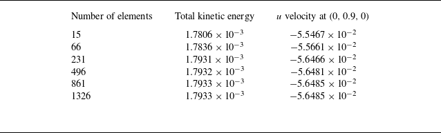
 u
u (0,0.9,0)
 Πc=297
 u0=0.2122
 u02
u02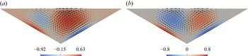
 Πc=297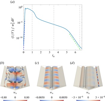
 wn2
wn2 Πc=934
 Lz=4
Lz=4 Q
Q tn=1
tn=1 tn=3.5
 tn=6.5
 wn
wn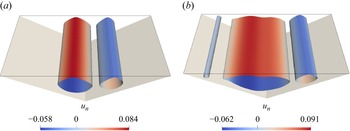
 Q
Q Πc=297
 Q
Q Πc=931
 Πc=1178
 Lz=2
Lz=2 wn
wn (0,0.9,0)
 log(y)
 |P1|
|P1| wn
wn
 Πc=1178
 |P1|
|P1| wn
wn
 Q
Q Πc=1040
 Πc=1559
 Πc=1819
 wn
wn Lz
Lz
 Πc=2180
 Lz=6
Lz=6 Q
Q wn
wn wn
wn z
z (0,0.9,0)
 wn
wn z
z (1.2,0.85,0)
 |P1|
|P1|
 Πc=3725
 Q
Q Q
Q
 Πc=6554
 Q
Q Q
Q
 Πc
Πc Πc≈2700
 Πc=297
 Pr=0.71
 Q
Q Q
Q
 Πc
Πc Nu∼Πcn
 n
n


 Open access

