2 Physical and numerical set-ups

We will investigate how the aforementioned two types of structured foils behave with respect to proton acceleration by means of two-dimensional PIC simulations with the smilei code (Derouillat et al. Reference Derouillat, Beck, Pérez, Vinci, Chiaramello, Grassi, Flé, Bouchard, Plotnikov and Aunai2018). The considered structures are visualized in figure 1(a–c). The reference target is a flat foil of thickness $d=100~\text{nm}$. It is composed of cold gold atoms, assumed to be 11-times ionized, with an ion number density of $5.85\times 10^{22}~\text{cm}^{-3}$. Simulations with different ionization states of gold atoms (up to 29-times ionized) were also performed but did not result in significant differences in proton spectra. A 10 nm thin proton–electron plasma layer with a number density of $1.74\times 10^{23}~\text{cm}^{-3}$ is added on the foil surfaces to model the hydrogen contaminants.

Figure 1.

Schematic representation of the flat foil (a), nanocone (b) and nanohole (c) targets. The targets are irradiated by the laser pulse from the left under an incidence angle of 45^°.

The nanocone target, sketched in figure 1(b), is composed of the above-mentioned flat foil coated with a distribution of cones, each having an opening angle of 44^° and a variable base size of $b$ (specific values will be set below). The nanohole target, displayed in figure 1(c), consists of the reference foil pierced by holes of the same width and location as the above nanocones. The surfaces of both types of structured targets are coated with a proton layer.

For the initialization of the nanocones’ positions, we choose the following model. Given the position $y_{1}$ of the first nanocone, the average distance $D=2.24b$ – motivated by practical considerations for target manufacturing – and the distance spread parameter $s=D/2$, the position of the $i$th nanocone is set iteratively to $y_{i}=y_{i-1}+D+(u-1/2)s$ as long as $y_{i}<y_{\max }$, where $y_{\max }$ is the maximal position and $u$ is a uniformly distributed random number taking values from 0 to 1. This leads to an average areal cone density of $\unicode[STIX]{x1D70C}=b/D=44\,\%$. The targets are located at $x=20~\unicode[STIX]{x03BC}\text{m}$.

The $p$-polarized laser pulse has a wavelength of $\unicode[STIX]{x1D706}=0.8~\unicode[STIX]{x03BC}\text{m}$ and a maximum intensity of $I_{0}=5\times 10^{19}~\text{W}~\text{cm}^{-2}$, corresponding to a normalized vector potential $a_{0}=4.8$ and a peak electric field of $194~\text{GV}~\text{cm}^{-1}$. It has Gaussian space and time profiles with a focal spot of $5~\unicode[STIX]{x03BC}\text{m}$ FWHM (full width half maximum) and a duration of 38 fs FWHM. It is incident on the target from the lower left-hand side, at 45^° from the surface normal. The peak intensity of the laser pulse reaches the foil after 175 fs in the simulation. In the following, we will set this as the time reference $t=0$.

The numerical discretization of the simulations is $\unicode[STIX]{x1D6FF}x=\unicode[STIX]{x1D6FF}y=5~\text{nm}$ and $\unicode[STIX]{x1D6FF}t=11.7~\text{as}$. We use 100 macro-particles per cell and per species in the bulk plasma, while the surface proton–electron layers are represented by 1000 macro-particles per cell and per species.

3 Enhancement of electron heating and ion acceleration

Periodic cone structures have been shown to enhance proton acceleration due to a modification of electron trajectories, hence maximizing laser absorption (Blanco et al. Reference Blanco, Flores-Arias, Ruiz and Vranic2017). It is thus interesting to investigate whether completely relaxing the restriction of periodicity would impact the acceleration process. Here, we consider a non-periodic arrangement of the structures. The cone and hole-base size in this section is fixed to be $b=300~\text{nm}$.

The strength of the rear-side sheath field that underpins TNSA, and which therefore determines the efficiency of the latter, is controlled by the energy density of the laser-generated hot electrons (Daido et al. Reference Daido, Nishiuchi and Pirozhkov2012; Macchi et al. Reference Macchi, Borghesi and Passoni2013). Figure 2(a) plots the energy spectrum of the electrons located in the vacuum region behind the rear side of the target, recorded at $t=175~\text{fs}$. Those electrons mainly account for the generation of the sheath electric field in the early stages of TNSA, when the approximation of the one-dimensional plasma expansion holds. Compared with the flat foil, both structured targets lead to a significantly increased number of relativistic electrons above 7 MeV, with the nanohole target yielding the largest enhancement – by approximately an order of magnitude.

Figure 2.

Energy spectra of electrons (a) and rear-side protons (b) from a flat foil (solid black), a nanocone (dashed-dotted yellow) and a nanohole (dashed red) target of $d=100~\text{nm}$ thickness. In (a), only electrons located in the vacuum behind the target backside are considered. Electron spectra are recorded at $t=175~\text{fs}$ and proton spectra at $t=455~\text{fs}$.

Figure 3.

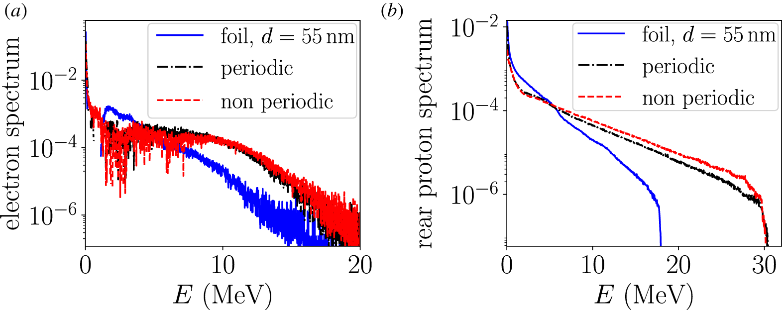
Energy spectra of the electrons (a) and rear-protons (b) from a flat foil (solid blue), a $d=100~\text{nm}$ periodic nanohole target (dashed-dotted black) and a $d=100~\text{nm}$ non-periodic nanohole target (dashed red). In (a), only electrons located in the vacuum behind the target backside are considered. Electron spectra are recorded at $t=175~\text{fs}$ and proton spectra at $t=455~\text{fs}$.

Figure 4.

(a)–(c) Maximum $\unicode[STIX]{x1D6FE}$ factor (locally averaged over the initial particle distribution) reached by electrons as a function of their initial position (yellow–red) and longitudinal electric field $E_{x}$ (units $m_{e}c\unicode[STIX]{x1D714}_{0}/e$, with $c$ the speed of light, $\unicode[STIX]{x1D714}_{0}$ the laser frequency, $m_{e}$ the electron mass and $e$ the elementary charge) at $t=0$, averaged over a laser period $T_{0}$ (blue–red). (d)–(f) Magnetic field $B_{z}$ (units $m_{e}\unicode[STIX]{x1D714}_{0}/e$) at $t=0$. The initial target densities are indicated in light grey, and correspond to $100~\text{nm}$-thick flat (a,d) nanohole (b,e) and nanocone targets (c,f) and the center of the laser spot on target is localized at $y=33.5~\unicode[STIX]{x03BC}\text{m}$.

A similar behaviour is found for the rear-side proton energy spectra, as plotted in figure 2(b) at $t=455~\text{fs}$. Both nanocone and nanohole targets give rise to much enhanced TNSA: the best performance is observed using nanoholes, with an almost doubled proton cutoff energy compared to that from the flat foil (${\sim}30~\text{MeV}$ protons versus ${\sim}17~\text{MeV}$).

Figure 3 demonstrates that the electron and proton spectra are almost the same for periodic and non-periodic targets, consistent with the conclusion reached by Klimo et al. (Reference Klimo, Psikal, Limpouch, Proska, Novotny, Ceccotti, Floquet and Kawata2011) when investigating irregular spherical structures. It is thus to be expected that the individual structuring units, rather than their periodic arrangement (possibly leading to the excitation of surface plasma waves), are responsible for the enhancement. This is a favourable result from an experimental perspective since it reduces the target manufacturing constraints.

Moreover, figure 3(a,b) presents the electron and rear-proton energy spectra obtained for a flat foil (blue solid line) of reduced thickness ($d=55~\text{nm}$) such that it contains the same total amount of matter as the $d=100~\text{nm}$ nanohole targets, whether periodic or not. This thinner flat foil produces particle energy spectra very similar to the $d=100~\text{nm}$ foil; hence, the enhanced performance of the nanohole targets cannot be ascribed to the direct effect of their reduced volume (or area in two dimensions) on the electron kinetic energy density (which would naturally increase assuming the same amount of laser energy is converted into hot electrons), but rather results from a strongly modified hot-electron dynamics.

Figure 5.

Trajectories of a few energetic electrons in the nanohole target (a) and the flat target (b). These electrons are selected randomly amongst those verifying $x>48~\unicode[STIX]{x03BC}\text{m}$ at $t=175~\text{fs}$, and as long as they have reached a threshold energy $E_{\text{th}}$ during the simulation, with $E_{\text{th}}=12~\text{MeV}$ in the nanohole case and $E_{\text{th}}=5~\text{MeV}$ in the flat target case. The initial target density is indicated in light grey. The colour of the trajectories (blue–red) represents the rate of change ($(p_{x}E_{x}+p_{y}E_{y})/\unicode[STIX]{x1D6FE}$) of electron energy (units $m_{e}^{2}c^{2}\unicode[STIX]{x1D714}_{0}/e$). Two trajectories of single electrons (black) are represented for each case in the different insets. The red dots indicate the initial positions of these particles.

In order to gain insight into the electron energization process in the nanostructured target, we record the maximum Lorentz factor $\unicode[STIX]{x1D6FE}$ reached by each electron during the simulation, and plot its locally averaged value as a function of the initial electron position (figure 4a–c). In the case of the flat foil (figure 4a), the resulting map shows that, as expected, most of the accelerated electrons originate from a ${\sim}25~\text{nm}$-thick surface layer at the directly irradiated front side of the target (with mean energies ${\sim}6~\text{MeV}$ being reached), and that rear-side electrons undergo negligible acceleration. In the case of the nanohole (figure 4b) and nanocone (figure 4c) targets, some of the highest energy electrons stem from additional regions, namely the nanohole walls and the nanocone sides. The nanostructuring of the target surface therefore increases the effective interaction area, leading to a larger number of hot electrons. The mean energy (${\sim}10~\text{MeV}$) reached by these electrons is also significantly larger than in the flat foil. These effects are supported by the local enhancement of the electrostatic field which appears when using nanostructured targets. The electrostatic field is indeed strongly enhanced at the corners of the nanoholes and at the tips of the nanocones, which correspond to the surfaces from which the most energetic electrons arise. Note that the value of the electrostatic field in these regions becomes of the same order as the laser field (figure 4d–f), which is also favourable for electron acceleration (Paradkar, Krasheninnikov & Beg Reference Paradkar, Krasheninnikov and Beg2012). Interestingly, when the target is nanostructured, the change in the laser field pattern on the front side of the target indicates a decrease in the laser reflection compared with the flat foil. This is confirmed by the reflection coefficient, which drops from $C_{R_{f}}=0.67$ to $C_{R_{c}}=0.15$ when adding the nanocones. While the flat and nanocone targets remain essentially opaque (with a transmission coefficient $C_{T_{f,c}}<0.02$), the laser light is partially transmitted through the nanoholes ($C_{T_{h}}=0.13$), as is evident from figure 4. Consequently, the absorption coefficient is lower in nanohole ($C_{A_{h}}=0.66$) than in nanocone targets ($C_{A_{c}}=0.83$). As further discussed below, this finding somewhat contradicts the widely shared notion that the absorbed laser energy fraction is the single figure of merit for TNSA.

This general behaviour can be complemented by examining individual electron trajectories. We focus on those high-energy electrons breaking through the target rear side, and therefore contributing to the accelerating sheath field. For this reason, figure 5 plots the trajectories of a sample of the most energetic electrons in both the flat and nanohole targets – with a lower energy cutoff for the selection of 12 MeV in the nanohole target (figure 5a) and of 5 MeV in the flat target case (figure 5b). Only those electrons that are located at a longitudinal position $x\geqslant 48~\unicode[STIX]{x03BC}\text{m}$ at $t=175~\text{fs}$ are selected. The colour of each trajectory is indexed on the rate of change of electron energy in the local electromagnetic fields. It can be seen that, on average, higher values are attained in the nanohole target. While the selected electrons mainly exhibit acceleration in the front- and rear-side vacuum regions, sizable energy transfer is also seen within the cavities, which is consistent with the laser being partially transmitted through the nanoholes (see figure 4e).

Figure 6.

Position of the front of the accelerating rear-proton layer at $t=175~\text{fs}$ for a flat foil (solid black), a nanocone (dashed-dotted yellow) and a nanohole (dashed red) targets of $d=100~\text{nm}$ thickness.

The sub-micron dense regions that make up the nanohole targets effectively behave as mass-limited targets (Psikal et al. Reference Psikal, Tikhonchuk, Limpouch, Andreev and Brantov2008; Buffechoux et al. Reference Buffechoux, Psikal, Nakatsutsumi, Romagnani, Andreev, Zeil, Amin, Antici, Burris-Mog and Compant-La-Fontaine2010), leading to efficient electrostatic confinement of the hot electrons. This is evidenced by the single particle trajectories displayed in the insets of figure 5: the nanohole target causes the electron to recirculate in both longitudinal (across the front and rear sides of the target) and transverse (across the nanohole walls) directions. A favourable consequence of this is a longer effective laser–electron interaction time. Also, the laser–electron interaction occurs under various geometrical conditions, and so with increased degrees of freedom. This results in a more complete exploration of the phase space, which ultimately allows the electrons to be accelerated to higher energies. Finally, being prevented from leaving the laser-irradiated region, the hot electrons are able to sustain a strong sheath field over longer times. The confinement of the hot electrons entails a reduced transverse extent of the sheath field, and therefore of the expanding proton cloud. This can be seen in figure 6, which shows the boundary of the proton cloud as resulting from the three target types, the nanohole target giving rise to a more narrow proton distribution. Compared to nanocone targets, the more localized and intense sheath fields induced in nanohole targets translate into lower numbers of accelerated protons but of higher energies, despite lower laser absorption. A drawback of nanohole targets, however, is the significant transverse sheath fields which build up at the sharp transverse vacuum–plasma interfaces, and tend to increase the divergence of the proton beam (measured to be approximately twice higher in nanohole targets than in flat foils).

4 Parametric scan for nanohole targets

Figure 7.

Particle density spectra of the rear-side electrons (a,d,g), front-side protons (b,e,h) and rear-side protons (c,f,i) from nanohole targets. The electron spectra are presented at $t=175~\text{fs}$, the front proton spectra at $t=315~\text{fs}$ and the rear proton spectra at $t=455~\text{fs}$. The foil thickness is $d=100~\text{nm}$ in (a–c), $d=300~\text{nm}$ in (d–f), $d=600~\text{nm}$ in (g–i). The nanohole diameter is varied in the range $0\leqslant b\leqslant 600~\text{nm}$, as indicated in the legend of each row.

We now perform a parametric scan where we vary the foil thickness $d$ and hole diameter $b$. Henceforth, we consider only the cases where the hole diameter is at least as large as the foil thickness, i.e. $b\geqslant d$.

Figure 7(a) presents the spectra of the rear-side electrons for foil thicknesses from 100 to 600 nm and various hole diameters. One can see that the electrons from the flat foil (grey line) reach lower energies than electrons from perforated foils, whatever the hole diameter. Especially above 5 MeV, perforated targets produce more high-energy electrons. The enhancement is very similar for hole sizes from 100 to 600 nm.

While we are mostly interested in the protons accelerated from the target back side, we also plot for completeness the energy spectra of the protons originating from the front side. Figure 7(b,c) presents the corresponding front (b) and rear (c) proton spectra. In both cases, the structuring significantly enhances the proton cutoff energies. While a 100 nm hole size already enhances the proton cutoff energy by approximately 40 %–50 %, the largest enhancements are reached for 300 to 600 nm diameter holes.

When increasing the gold foil thickness, the trends remain the same (see figure 7d–i). The presence of the holes increases the number of high-energy electrons and boosts the proton energy by approximately a factor of 2. The thinner the gold foil, the higher the proton energies. However, while this nanohole structuring can be used for all target thicknesses, the relative improvement is slightly more pronounced for thicker foils (by 95 % at $d=300~\text{nm}$ versus 70 % at $d=100~\text{nm}$).

The PIC simulation results suggest that as long as the parameters are in the above-described range leading to enhancement, they can be freely chosen depending on other experimental constraints, e.g. ease of handling and fabrication.

Note that our simulations consider sharp-gradient targets, meaning that they do not address the possible influence of finite preplasmas caused by laser prepulses. The generation of a significant preplasma would modify the picture: the holes might be filled with electrons before the arrival of the main pulse, thus suppressing the benefit of the target structuring. Larger hole diameters may then be preferable under actual experimental conditions.

Figure 8.

Rear-side electron and proton energy spectra under conditions similar to those of figure 2, but with different hole densities $\unicode[STIX]{x1D70C}$ according to the legends in (a) and (b).

The areal density of the holes can be expected to play a role in enhancing TNSA. Figure 8 displays the energy spectra of the rear-side electrons and protons obtained from 100 nm thick nanohole targets of nanohole density varying in the range $0\leqslant \unicode[STIX]{x1D70C}\leqslant 67\,\%$. An optimum electron heating and proton acceleration is reached when almost half of the surface area is covered by the holes. However, already for a density of approximately 20 %, a notable increase in the cutoff energy is reached.

The optimum is likely formed by two counteracting effects. On the one hand, when increasing the hole density, the mechanisms described in § 3 further develop: more electrons can get an energy boost due to the increase in the interaction surface and recirculation. On the other hand, raising the hole density reduces the effective target volume, eventually resulting in higher laser transmission, and therefore weaker laser–target coupling. To mitigate the latter effect, one could use thicker foils instead of the considered 100 nm thin foils. However, this solution is limited by the fact that the proton cutoff energy tends to be reduced when the nanohole target gets thicker – in the same manner as for the standard flat-foil target.