


Introduction
In 1860, John Phillips made one of the earliest known attempts to estimate global Phanerozoic biodiversity (Phillips Reference Phillips1860; Miller Reference Miller2000). In his largely qualitative estimate, Phillips identified two major diversity declines, one at the end of the Paleozoic and one at the end of the Mesozoic, and two major diversity increases, one during the early Paleozoic and one during the Cenozoic. Newell (Reference Newell1952) used a more taxonomically and temporally explicit dataset to identify broadly similar patterns, but with more temporal structure. Cutbill and Funnell (Reference Cutbill and Funnell1967) binned the number of taxa to the stage level, enabling a more detailed quantitative analysis on the Phanerozoic diversity and identifying several peaks in marine extinction. Sepkoski (Reference Sepkoski1981) assembled a global compendium of marine animal genus first and last appearances, allowing more nuanced reconstructions of diversity, turnover, and faunal composition that led to the quantitative identification of three marine evolutionary faunas (Sepkoski Reference Sepkoski1981) and five major mass extinctions (Raup and Sepkoski Reference Raup and Sepkoski1982). Analogous compilations for the non-marine fossil record (Benton et al. Reference Benton, Dunhill, Lloyd and Marx2011, Reference Benton, Ruta, Dunhill and Sakamoto2013) demonstrated a protracted and largely uninterrupted increase in diversity from a Late Ordovician/Silurian low to a Recent high.
Although most such compilations of fossil taxonomic diversity and turnover have yielded broadly similar temporal patterns that suggest a biological signal is present, it is well known that sampling effort and fossil preservation can significantly distort macroevolutionary patterns (Raup Reference Raup1972, Reference Raup1976; Benton and Emerson Reference Benton and Emerson2007). Indeed, overcoming sampling-related biases was one of the primary motivations for the creation of the Paleobiology Database (PBDB), a geographically and taxonomically explicit global compilation of fossil occurrences that allowed for the development and application of sampling standardization approaches, among other things (e.g., Alroy et al. Reference Alroy, Marshall, Bambach, Bezusko, Foote, Fürsich, Hansen, Holland, Ivany, Jablonski, Jacobs, Jones, Kosnik, Lidgard, Low, Miller, Novack-Gottshall, Olszewski, Patzkowsky, Raup, Roy, Sepkoski, Sommers, Wagner and Webber2001, Reference Alroy, Aberhan, Bottjer, Foote, Franz, Harries, Hendy, Holland, Ivany, Kiessling, Kosnik, Marshall, McGowan, Miller, Olszewski, Patzkowsky, Peters, Loïc, Wagner, Bonuso, Borkow, Brenneis, Clapham, Fall, Ferguson, Hanson, Krug, Layou, Leckey, Sabine, Powers, Sessa, Simpson, Adam and Visaggi2008; Finnegan et al. Reference Finnegan, Anderson, Harnik, Simpson, Tittensor, Byrnes, Finkel, Lindberg, Liow, Lockwood, Lotze, McClain, McGuire, O'Dea and Pandolfi2015; Bush et al. Reference Bush, Hunt and Bambach2016; Klompmaker et al. Reference Klompmaker, Kowalewski, Huntley and Finnegan2017; Sansom et al. Reference Sansom, Choate, Keating and Randle2018; Chiarenza et al. Reference Chiarenza, Farnsworth, Mannion, Lunt, Valdes, Morgan and Allison2020; Song et al. Reference Song, Kemp, Tian, Chu, Song and Dai2021; Raja et al. Reference Raja, Dunne, Matiwane, Khan, Nätscher, Ghilardi and Chattopadhyay2022; Siqueira et al. Reference Siqueira, Kiessling and Bellwood2022; Spiridonov and Lovejoy Reference Spiridonov and Lovejoy2022).
Despite the utility of the PBDB, fossil occurrences and the macroevolutionary signals they reveal are embedded in the sedimentary rock record, which itself exhibits significant temporal variability in quantity and quality (Ronov et al. Reference Ronov, Khain, Balukhovsky and Seslavinsky1980; Berry and Wilkinson Reference Berry and Wilkinson1994; Peters Reference Peters2006b; Meyers and Peters Reference Meyers and Peters2011; Peters and Husson Reference Peters and Husson2017). Covariation between temporal patterns in the sedimentary rock and fossil records has been demonstrated many times and in many different ways (Raup Reference Raup1972, Reference Raup1976; Holland Reference Holland2000; Peters and Foote Reference Peters and Foote2001, Reference Peters and Foote2002; Smith Reference Smith2001; Smith et al. Reference Smith, Gale and Monks2001; Peters Reference Peters2005, Reference Peters2006a; Peters and Ausich Reference Peters and Ausich2008; Alroy Reference Alroy2010; Heim and Peters Reference Heim and Peters2010, Reference Heim and Peters2011; Benton et al. Reference Benton, Dunhill, Lloyd and Marx2011, Reference Benton, Ruta, Dunhill and Sakamoto2013; Lloyd et al. Reference Lloyd, Smith and Young2011; Rook et al. Reference Rook, Heim and Marcot2013; Zaffos et al. Reference Zaffos, Finnegan and Peters2017). The traditional view is that the sedimentary record is dominated by postdepositional destruction and modification, leading to variability and an expected decrease in quantity and quality with increasing age, both of which can distort macroevolutionary patterns (e.g., Darwin Reference Darwin1859; Huxley Reference Huxley1862; Foote Reference Foote2000; Peters and Foote Reference Peters and Foote2001, Reference Peters and Foote2002; Smith Reference Smith2001; McGowan and Smith Reference McGowan and Smith2008). However, it has also been suggested that variability in the sedimentary rock record reflects changes in the state of the Earth system, such as the extent of continental flooding, which can affect macroevolutionary outcomes (Newell Reference Newell1956, Reference Newell1959 Reference Newell1962, Reference Newell1963; Valentine and Moores Reference Valentine and Moores1970, Reference Valentine and Moores1972; Sepkoski Reference Sepkoski1976; Ronov et al. Reference Ronov, Khain, Balukhovsky and Seslavinsky1980; Raup and Sepkoski Reference Raup and Sepkoski1982; Peters and Foote Reference Peters and Foote2002; Peters Reference Peters2005, Reference Peters2006a, Reference Peters2007; Peters and Heim Reference Peters and Heim2010, Reference Peters and Heim2011; Butler et al. Reference Butler, Benson, Carrano, Mannion and Upchurch2011; Hannisdal and Peters Reference Hannisdal and Peters2011; Heim and Peters Reference Heim and Peters2011; Zaffos et al. Reference Zaffos, Finnegan and Peters2017).
In addition to the preservation and availability of sedimentary rock, inconsistencies in the intensity of geographic sampling and geochronological correlation challenges have also contributed to the distortion of macroevolutionary patterns, particularly in ostensibly global databases like Sepkoski's compendium and the PBDB (Sheehan Reference Sheehan1977; Crampton et al. Reference Crampton, Beu, Cooper, Jones, Marshall and Maxwell2003; Raja et al. Reference Raja, Dunne, Matiwane, Khan, Nätscher, Ghilardi and Chattopadhyay2022). For example, Kiessling (Reference Kiessling2005) found that socioeconomic factors are responsible for some amount of sampling bias in Phanerozoic fossil reefs, with higher gross domestic product (GDP) correlated with more ancient reef data. Other studies have found that countries with more developed economies, political stability, and higher political influence, especially those in North America and Europe, tend to be more productive in generating paleontological publications that can be included in global databases (Amano and Sutherland Reference Amano and Sutherland2013; Hughes et al. Reference Hughes, Orr, Ma, Costello, Waller, Provoost, Zhu and Qiao2021). Notably, Raja et al. (Reference Raja, Dunne, Matiwane, Khan, Nätscher, Ghilardi and Chattopadhyay2022) found that there is a large imbalance between fossil data from developed and developing countries in the PBDB, with a vast majority of global fossil data contributed by high- or upper-middle-income countries.
Here, we assess temporal and spatial variability in the distribution of PBDB fossil occurrences within the geological context that is provided by the global surface-expressed sedimentary rock record in Macrostrat (https://macrostrat.org). Our primary motivation is to answer three questions: First, given the spatial and temporal variability that is inherent in the sedimentary rock record, how much better sampled are North America and Europe than other regions? Second, how consistent and strong are the expected positive correlations between fossil occurrences, generic diversity derived from those occurrences, and geological map area of sedimentary rock units yielding fossil occurrences? Third, if the rock record of other geographic regions yielded occurrences in numbers comparable to those of North America and Europe, how many more fossil occurrences would be added to the PBDB, and what would be the effect of these new occurrences? In answering these questions, we seek to provide geologically calibrated expectations for the global Phanerozoic fossil record and to provide a tangible, geological foundation upon which to assess geographic disparities in fossil occurrences in the PBDB.
Datasets and PBDB Collection–Geological Map Polygon Matching
At the time of this analysis (February 2022), we retrieved data for 224,107 fossil collections from the PBDB, which included their respective geographic coordinates, maximum and minimum age estimates (in Ma), inferred depositional environments, and the number of occurrences and list of genera. These data can be retrieved from the current PBDB using the application programming interface (Peters and McClennen Reference Peters and McClennen2016). The PBDB dataset we used here contains 1,547,258 total occurrences and 66,782 genera from both marine and terrestrial environments (see Supplementary File for the formatted raw data used in this analysis).
We obtained global geological map polygons from the Macrostrat database at the “small” scale (Peters et al. Reference Peters, Husson and Czaplewski2018), with corresponding spatial information and metadata, including top and bottom ages (in Ma), and lithologies (Fig. 1A). A total of 124,081 map polygons are in the dataset, of which 55,969 are Phanerozoic sedimentary polygons (see Supplementary File for the formatted raw data used in this analysis). All igneous, metamorphic, and Precambrian polygons are either excluded or identified as such in all of our analyses. Map polygons with identical metadata (name, age, lithology, etc.) from the same map source (Asch Reference Asch2003; Harrison et al. Reference Harrison, St-Onge, Petrov, Strelnikov, Lopatin, Wilson, Tella, Paul, Lynds, Shokalsky and Hults2008; Garrity and Soller Reference Garrity and Soller2009; Raymond et al. Reference Raymond, Gallagher, Shaw, Yeates, Doutch, Palfreyman and Blake2010; Thiéblemont Reference Thiéblemont2016; Gómez et al. Reference Gómez, Schobbenhaus and Montes2019) are grouped into distinct map units, which may comprise many individual, spatially disconnected but proximal map polygons. A total of 3464 distinct such map units are in the global map dataset. For an online interactive version of the map data used here (as well as map data not used here but that are available at different scales of resolution), see https://macrostrat.org/map/#x=0&y=0&z=3.47 (zoom level, “z,” must be between 3 and 6 to see the same map sources and polygons used in this research).
Geological map and fossil collections. A, “Small”-scale geological map from the Macrostrat database (Precambrian and igneous/metamorphic rocks are separately colored). B, Matched PBDB collections colored by the color scheme of their matched Macrostrat map polygons. C, Unmatched collections colored by their age in the PBDB and the standard colors for periods.
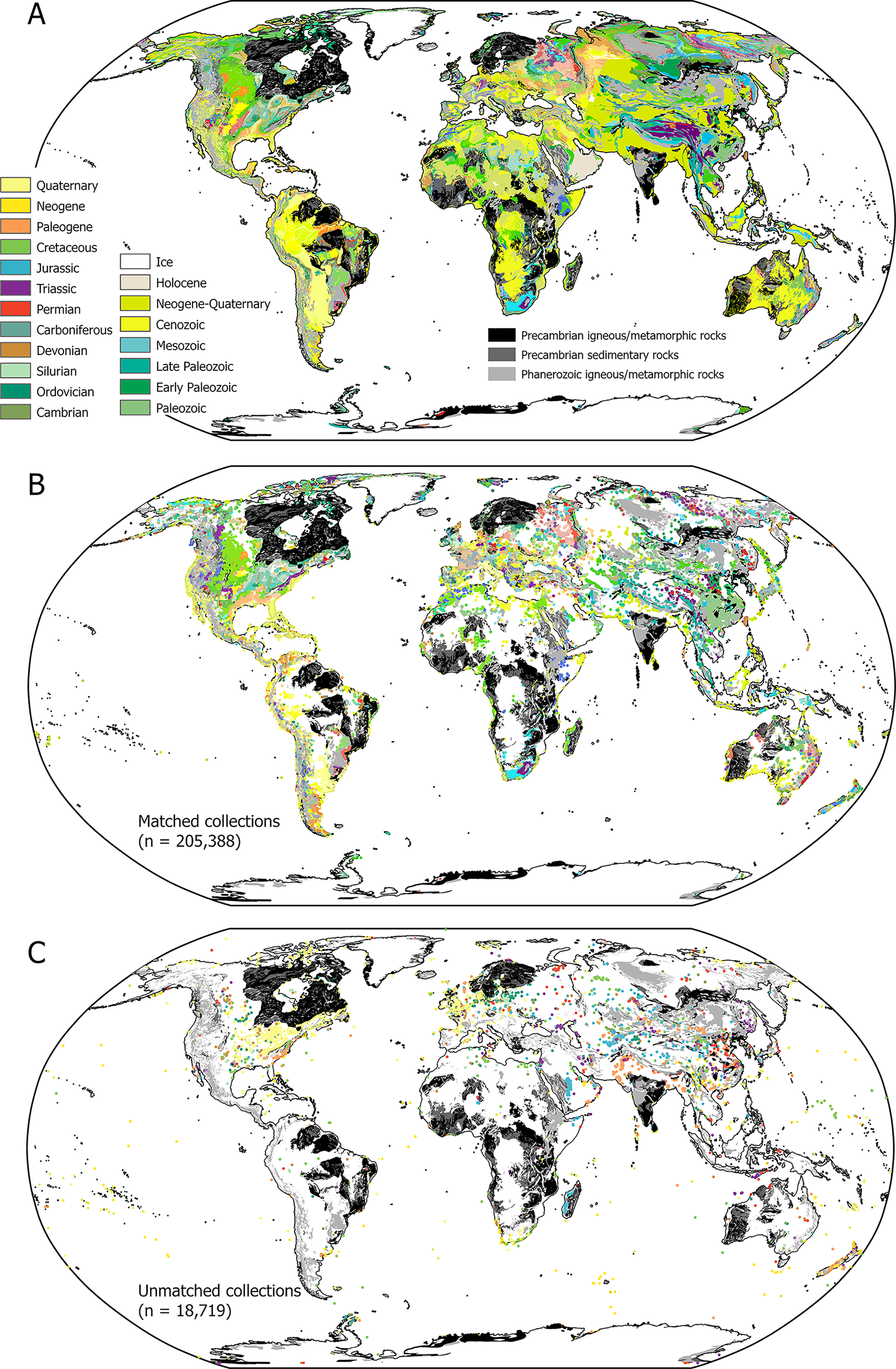
With the above raw data in hand, we used ArcGIS Pro and its companion ArcPy library for Python to intersect the Macrostrat map data and PBDB fossil data based on their spatial and temporal attributes (geographic coordinate system of WGS84). We excluded 869 fossil collections that are more than 150 km from any land as indicated by the map data (Supplementary Fig. S1), which left 223,238 collections. Fossil collections falling within a sedimentary/metasedimentary map polygon that also have overlapping age estimates are directly matched to their containing polygon; 49% of PBDB fossil collections are matched in this way. Each map polygon then acquires all the information corresponding to the matched collection(s), including the type of environment and the number of occurrences and genera. If the fossil collection's age ranges and the polygon it is located in do not overlap, or if a fossil collection is outside any sedimentary polygon, then sedimentary polygons with overlapping age ranges are searched for within a radius of 150 km. This 150-km buffer was used after testing different distances; it was found to achieve a balance between the precision of spatial matching and the spatial uncertainties in fossil data. Key results are not sensitive to this convention. If within the 150-km tolerance there are polygons that match a collection based on age, then the closest polygon to the collection is assigned. An additional 42% of the PBDB fossil collections can be matched to a map polygon after this second round of intersection, resulting in a total of 90.7% polygon-matched collections. Next, a temporal buffer of 2 Myr is allowed for the remaining unmatched fossil collections (Supplementary Fig. S1). This results in another 1% of collections being matched, for a combined total of 92% (n = 205,388; Fig. 1B). Of the remaining 8% (n = 17,850) of unmatched collections, 35.4% are from the Cenozoic (17.1% are Quaternary); 30.8% are Mesozoic; and 33.8% are Paleozoic (Fig. 1C). The most likely reasons for these collections being left unmatched include their derivation from geological units that are not mapped at the scale of resolution used here (e.g., Quaternary deposits in much of the Midwest of the United States), errors in the coordinates entered in the PBDB, and discrepancies and errors in the ages of PBDB collections and/or geological map units.
Most fossil collections have an inferred depositional environment in the PBDB, and we classified all types of environments into marine and terrestrial categories (about 6500 collections with unknown environments are omitted from the analysis). For all polygons that match at least one fossil collection, we count the number of marine and terrestrial collections they contain and calculate the fraction of marine collections (Fig. 2A). A map polygon is defined as marine if more than 60% of the contained collections are marine; a map polygon is defined as terrestrial if less than 40% of contained collections are marine; if the marine collections in a map polygon have a fraction between 40% and 60%, then the polygon is defined as a mixed marine/non-marine polygon (Fig. 2B). Because some map units consist of relatively thick succession of marine and terrestrial sedimentary deposits, mixed proportions of PBDB environments are expected in many cases.
Map of depositional environments based on PBDB collection matches. A, The fraction of marine collections in each polygon with at least 1 matched collection. B, Classification of inferred environments of each polygon based on 40% and 60% cutoffs of the marine fraction.

All of the above operations were conducted at the granular level of individual map polygons. As mentioned, individual polygons from the same map source that have identical metadata can be grouped into the same geological map unit. In our dataset, there are 3464 such sedimentary/metasedimentary map units of Phanerozoic age. For each distinct map unit, which may consist of multiple individual polygons, we sum the number of fossil occurrences recorded in each of the individual polygons to obtain the number of occurrences for that map unit; the unique genera in each polygon are also summed for each map unit. Finally, the number of marine and terrestrial collections are tabulated in each distinct map unit and the same fraction cutoffs (40% and 60%) are used for defining the marine, mixed, and terrestrial map units.
Results
The “small”-scale geological map of the world compiled by Macrostrat (Fig. 1A) exhibits spatial variability in the distribution and age of sedimentary deposits. For example, Precambrian-aged rocks and igneous rocks occupy significant fractions of the area of some continental blocks, notably in northern North America, South America, and Africa (Fig. 1). Neogene/Quaternary sedimentary deposits are also very widespread in some of these same regions, resulting in somewhat different area–age relationships across continental blocks (see below).
At the granular polygon level (Fig. 3A), the proportion of area among Phanerozoic sedimentary polygons that is matched to at least one fossil collection is between 0.7 and 0.8 for all ages, while at the distinct map unit level (Fig. 3B), the same matched proportion is always close to 1.0; that is, most sedimentary rock units mapped at this scale appear to yield at least some fossils. At the granular polygon level, the total area of sedimentary polygons with at least 1 matched collection is about 64.8 million km2 (74% of all Phanerozoic sedimentary area), including 29 million km2 of marine polygons, 30.8 million km2 of terrestrial polygons, and 5 million km2 of mixed polygons based on our classifications of environments (Fig. 3C). After integrating to the distinct map unit level (Fig. 3D), the map area of mixed marine/non-marine environments shows a significant increase in area toward the Recent, whereas the area of marine environments shows a decrease toward the Recent. The total map area at the distinct map unit level with at least 1 matched collection is about 83.5 million km2 (95% of all Phanerozoic sedimentary area), including 26.9 million km2 (34%) of marine units, 2.9 million km2 (3%) of terrestrial units, and 53.7 million km2 (61%) of mixed units.
Matched and unmatched geological map areas vs. age showing overall area–age patterns. A, Matched and unmatched granular polygons. B, As in A, but for distinct map units. Matched fraction in A and B shown by blue curves and blue axis labels. C, Inferred environments of deposition for geological map area based on PBDB collection matches to individual granular polygons. D, As in C, but with environments determined on the basis of distinct map units matched to PBDB collections. In both C and D, environments are determined by the fraction of fossil environments in each polygon or unit (see text for criteria). Polygons or map units with no matched fossil collection have an unknown environment. Cm, Cambrian; O, Ordovician; S, Silurian; D, Devonian; C, Carboniferous; P, Permian; Tr, Triassic; J, Jurassic; K, Cretaceous; Pg, Paleogene; N, Neogene.

In North America and Europe, PBDB collections are so densely distributed that they effectively form a crowd-sourced, point-based geological map when collection points are colored by age to match the conventions used in the global geological map (Fig. 1B). There are similar collection densities to a limited extent in other regions of the world, but large areas of sedimentary deposits are devoid of PBDB fossil collections, and many of these areas correspond to Neogene and Quaternary map units, most of which are non-marine. Unmatched PBDB collections are small in number and rather diffusely distributed (Fig. 1C). The geographic distribution of marine, non-marine, and mixed sedimentary deposits, based on the environments assigned to matched PBDB fossil collections, are also heterogeneous (Fig. 2), with, for example, large areas of South America and Africa being predominately non-marine versus the largely marine coverage in much of North America and Europe.
In general, the fraction of PBDB marine fossil collections that are matched to Macrostrat map polygons is relatively stable as a function of age in the Phanerozoic, hovering around 0.9 with relatively low match fractions during the Cambrian, late Permian–Triassic, Late Jurassic, and Cenozoic (Fig. 4A). The match fraction of terrestrial fossil collections shows an overall slight decreasing trend toward the Recent. In the Cambrian and Ordovician, there are almost no terrestrial collections, which broadly mirrors the pattern of non-marine sediment rock abundance (Peters and Husson Reference Peters and Husson2017). From the Devonian to early Permian, the match fraction of terrestrial fossil collections is close to 1.0. It starts to decline in the Mesozoic, falling below 0.8 twice in the mid-Jurassic and the mid-Cretaceous respectively. It then has a weak upward trend in the Cenozoic, returning to 0.9 or higher, except for one trough in the late Paleocene (Fig. 4B).
Time series of matched and unmatched collections within marine and terrestrial environments using PBDB age estimates. A, Number of marine collections vs. age and the fraction of those collections matched to map units (blue). B, Number of terrestrial collections vs. age and the fraction of those collections matched to map units (blue). C, Stack plot of the number of marine (blue) and terrestrial (tan) fossil occurrences. D, As in C, but for genera. E, Time series of global occurrences normalized by global sedimentary map area. F, As in E, but for distinct genera normalized by global sedimentary map area. Cm, Cambrian; O, Ordovician; S, Silurian; D, Devonian; C, Carboniferous; P, Permian; Tr, Triassic; J, Jurassic; K, Cretaceous; Pg, Paleogene; N, Neogene.

There is no significant increase in face-value, genus-level diversity (sampled-in-bin) in the aggregate marine fossil record, but distinct declines can be seen at the Ordovician/Silurian boundary, Late Devonian, end Permian, Late Triassic, and the Cretaceous/Paleogene boundary, which correspond to the pattern of known mass extinctions (Fig. 4C,D). In the time series of fossil occurrence and genus counts normalized by map area (Fig. 4E,F), marine fossil occurrences as well as generic diversity show an overall upward trend through the Phanerozoic, which is particularly evident at the genus level.
There is an overall upward trend in terrestrial fossil occurrences, with a very pronounced peak centered around the Late Cretaceous (Fig. 4C). This may be due to the supersampling of some Maastrichtian–Campanian formations in North America, which have good accessibility and contain large and abundant dinosaur fossils (Kindler and Darras Reference Kindler and Darras1997; Brown et al. Reference Brown, Evans, Campione, O'Brien and Eberth2013). The Late Cretaceous plateau in occurrences is not mirrored at the genus level. Instead, there is a peak in the Paleogene, probably associated with hot spots of fossil sampling in the vicinity of the hyper-diverse Green River Formation in the western United States (e.g., Eugster and Surdam Reference Eugster and Surdam1973; Buchheim Reference Buchheim, Renaut and Last1994; Smith et al. Reference Smith, Carroll and Singer2008; Johnson et al. Reference Johnson, Birdwell, Mercier and Brownfield2016). However, in the time series of occurrences and genera normalized by map area (Fig. 4E,F), an increasing trend in the terrestrial data is not obvious; if anything, there is a decreasing trend toward the Recent.
Correlations between Map Area, Occurrences, and Genera
At the granular polygon level, there is a moderately weak positive correlation between geological map area and the number of occurrences (Fig. 5A, Pearson's r = 0.24, Spearman's rho = 0.22, p-value < 0.01), but the positive correlation becomes stronger when integrated at the distinct map unit level (Fig. 5B, Pearson's r = 0.40, Spearman's rho = 0.54, p-value < 0.01). If the data are tabulated into 10-Myr time bins, there is an even stronger positive correlation between map area and the number of fossil occurrences (Fig. 5C, Pearson's r = 0.72, Spearman's rho = 0.60, R 2 = 0.66). There is also a positive correlation between the number of fossil occurrences and map area at the level of geological periods (Fig. 5D). The positive correlation is quite strong between the Cambrian and Paleogene (Pearson's r = 0.74, Spearman's rho = 0.70, R 2 = 0.55), but the Neogene and Quaternary periods, which contain large terrestrial polygons with much fewer occurrences than expected, depart from the Phanerozoic trend, resulting in a reduced positive correlation overall (Fig. 5D, Pearson's r = 0.37, Spearman's rho = 0.68, R 2 = 0.15). Correlations also exist between map area and the number of genera (Fig. 5E–H). At the granular polygon level, there is a moderately weak positive correlation between a map polygon area and the number of genera contained in the polygon (Fig. 5E, Pearson's r = 0.22, Spearman's rho = 0.21, p-value < 0.01), while at the distinct map unit level, the positive correlation is stronger (Fig. 5F, Pearson's r = 0.48, Spearman's rho = 0.55, p-value < 0.01). Similarly, if the data are tabulated by time bins of 10 Myr, there is a strong positive correlation between map area and number of genera (Fig. 5G, Pearson's r = 0.63, Spearman's rho = 0.78, R 2 = 0.69). At the geological period level, there is a very strong positive correlation between map area and number of genera from the Cambrian to Paleogene (Pearson's r = 0.95, Spearman's rho = 0.83, R 2 = 0.90). Similar to the occurrence data, the genus-level diversity data of Neogene and Quaternary do not follow this pattern, resulting in a moderate positive correlation for the Phanerozoic overall (Fig. 5H, Pearson's r = 0.47, Spearman's rho = 0.78, R 2 = 0.22).
Scatter plots and Pearson's r values of occurrences and genera vs. map area. A, Occurrences vs. granular polygon area. B, Occurrences vs. distinct map unit area. C, Occurrences vs. map area in 10-Myr time bins. D, Occurrences vs. map area in geological periods. E, Genera vs. granular polygon area. F, Genera vs. distinct map unit area. G, Genera vs. map area in 10-Myr time bins. H, Genera vs. map area in geological periods. Cm, Cambrian; O, Ordovician; S, Silurian; D, Devonian; C, Carboniferous; P, Permian; Tr, Triassic; J, Jurassic; K, Cretaceous; Pg, Paleogene; N, Neogene; Q, Quaternary.

We found no significant correlation between the number of fossil occurrences/genera and the age of map polygons/units. The Pearson's r between the midpoint age of a map unit and the number of fossil occurrences is −0.01 at the granular polygon level and −0.08 at the distinct map unit level. Similarly, the Pearson's r between the midpoint age of a map unit and the number of genera is 0.01 at the granular polygon level and −0.12 at the distinct map unit level. It is also worth noting that there is a very strong positive correlation between the number of occurrences and the number of genera within the same map unit, both at the granular polygon level (Pearson's r = 0.68, Spearman's rho = 0.96, p-value < 0.01) and at the distinct map unit level (Pearson's r = 0.81, Spearman's rho = 0.99, p-value < 0.01). Thus, the number of occurrences within map units is largely redundant with the number of genera. For simplicity in this analysis, we will focus on the number of occurrences within map units.
Sampling in North America and Europe in Comparison to Other Regions
At the granular geological map polygon level, the highest raw counts of fossil occurrences per map polygon are in North America and Asia (Fig. 6A). Clusters of fossil-rich North American polygons are found in the regions corresponding to the Cretaceous Interior Seaway as well as the Late Cretaceous to early Paleogene around the Atlantic Seaboard and Mississippi Embayment in the United States. During the Cretaceous, these areas were predominately shallow-marine and coastal environments. In addition, there are several other fossil hot spots in North America. One example is the Late Ordovician around the tristate borders between Kentucky, Ohio, and Indiana, which have map polygons yielding large numbers of occurrences. This is one of the most fossiliferous areas in the world with well-exposed fossil-rich outcrops (e.g., Ausich Reference Ausich, Hess, Ausich, Brett and Simms1999; Schramm Reference Schramm2011; Harris et al. Reference Harris, Alley, Fine and Deline2019). Another one is the Late Devonian strata including the Catskill Formation in upstate New York and northern Pennsylvania, where abundant vertebrate, invertebrate, and plant fossils have been recovered (e.g., Woodrow and Isley Reference Woodrow and Isley1983; Woodrow Reference Woodrow, Woodrow and Sevon1985; Broussard et al. Reference Broussard, Trop, Benowitz, Daeschler, Chamberlain and Chamberlain2018). Quaternary sediments along the Atlantic coast of eastern North America also yield large amounts of fossils. The rest of the fossil-rich map polygons are mostly located in Asia, but the difference here is that the high numbers of fossil occurrences are a direct result of the coarser spatial and temporal resolution of the map data in that region (Fig. 1A). One of the Asian polygons with a large number of matched fossil occurrences is a sedimentary polygon in southern China resolved only to the “Paleozoic”; it contains several fossil-rich, well-studied units, like the Cambrian Wangcun section in Hunan (e.g., Peng and Robison Reference Peng and Robison2000), the Ordovician Meitan Formation in Guizhou (e.g., Wang et al. Reference Wang, Wei, Luan, Wu, Percival and Zhan2020), the Silurian units of the Huaying Mountains in Sichuan (e.g., Wang et al. Reference Wang, Zhan, Deng and Liu2013), the Devonian Lali section in Guangxi (e.g., Hou Reference Hou1986; Zhang et al. Reference Zhang, Over, Ma and Gong2019), the Carboniferous Yashui section in Guizhou (e.g., Lin et al. Reference Lin, Wang, Edouard and Aretz2012), and the Permian Zhongzhai and Zhongying sections in Guizhou (e.g., Zhang and He Reference Zhang and He2008; Wu et al. Reference Wu, Zhang and Sun2019). These strata range from Cambrian to Permian in time (between 541 and 251.9 Ma) and are located in various Chinese provinces across a considerably large region. The coarse temporal scale and the relatively large size of this southern China polygon contribute to its high number of matched fossil occurrences. The other fossil-rich Asian polygon is the largest single polygon in the map dataset: a Cenozoic polygon with an age range from the Neogene to the present covering the drainage basins of the upper Ob, upper Irtysh, Amu Darya, Syr Darya, Indus, Ganges, lower Brahmaputra, and Irrawaddy Rivers, which stretch from southern Siberia, through Central Asia and northern India, to Myanmar. Its size is close to 5 million km2, which is bigger than the entirety of Europe (as defined in Fig. 7A). Outside North America and Asia, there is another very big Quaternary polygon (>2 million km2) in South America centered on the Parana-La Plata river plain. It also contains more fossil occurrences compared to other South American polygons. There is also a big Quaternary polygon of similar size in northern Africa, but because fossil occurrences are generally sparse in that region, it does not stand out in Figure 6A.
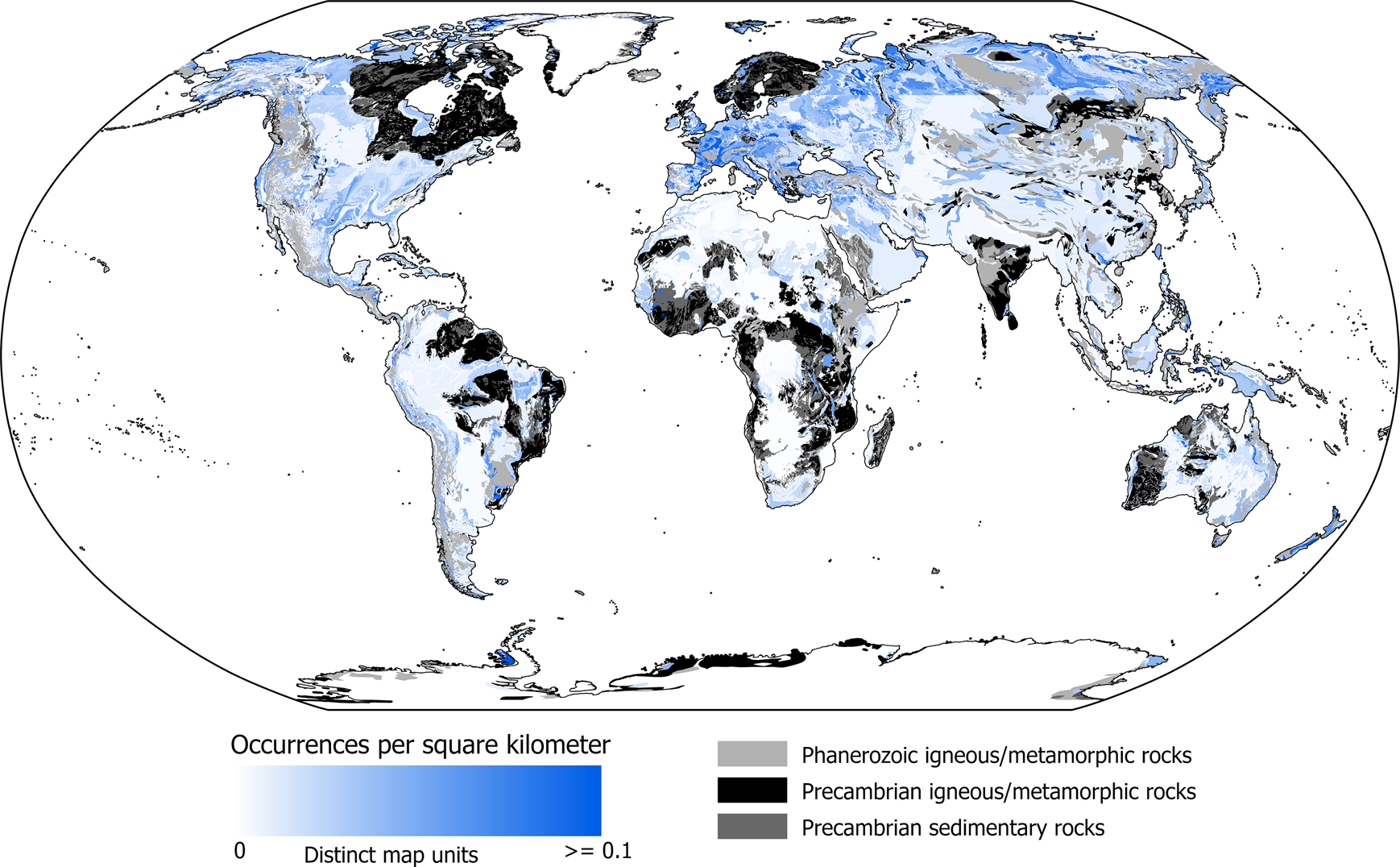
Observed spatial distribution and density of fossil occurrences within sedimentary polygons. A, Raw number of occurrences in each map polygon. B, Occurrences per square kilometer in each map polygon. C, Raw number of occurrences in each distinct map unit. D, Occurrences per square kilometer in each distinct map unit. D shows the preferred estimate.

Regional subdivisions, sedimentary map area, and occurrences per map area using map age estimates. A, The regional division of study areas used here. B, Sedimentary rock area through time in each of these regions. C, Occurrence per square kilometer in these different regions tabulated by polygon ages. Cm, Cambrian; O, Ordovician; S, Silurian; D, Devonian; C, Carboniferous; P, Permian; Tr, Triassic; J, Jurassic; K, Cretaceous; Pg, Paleogene; N, Neogene.

To reduce the effect of absolute polygon size and more accurately capture spatial variation in sampling intensity relative to sedimentary map area, we normalize the number of occurrences in each polygon by the polygon area; area and occurrences show a generally linear relationship (Supplementary Fig. S2). The result of this normalization is shown by Figure 6B. Most of the hot spots attributable to very large polygon sizes in Asia and South America disappear after normalization; these polygons are not particularly fossil rich in comparison to their very large size. The Paleozoic polygon in southern China still stands out (Fig. 6B) due to a long temporal duration that encompasses many fossiliferous units, but it is not as prominent as it is in the raw occurrence data (Fig. 6A). In contrast, most of the previous hot spots in North America still stand out, while some smaller North American polygons are also evident. Examples include the Eocene sediments in the Green River, Wind River, and Bighorn Basins of Wyoming, and some other small basins in the Basin and Range province and California. North American and European map units do have the smallest median sizes (Table 1), indicating relatively good map coverage in the region. European polygons do not have higher raw occurrences numbers but clearly show higher numbers of occurrences per square kilometer (Fig. 6B). Polygons in England, France, Germany, Switzerland, Belgium, and southern Poland have especially high occurrences per square kilometer. Outside North America, Europe, and southern China, there are several small hot spots, including some in Tunisia, Morocco, Japan, Russia, Argentina, and Australia. However, most of the rest of the world is not comparably sampled compared with North America and Europe when occurrences are normalized by sedimentary area.
Number (n) of Phanerozoic distinct map units with at least 1 occurrence and the median area of distinct map units (in km2) in each region.

For regional analyses, we divided the global map data into seven areas (Fig. 7A) that do not correspond exactly to realistic natural or political boundaries. We let the eastern boundary of “Europe” follow the eastern borders of Romania, Hungary, Slovakia, Poland, and Finland, as these countries and the area west of them have significantly better fossil-sampling rates (Fig. 6D). The western boundary of “Asia” reflects a significant change in the spatial resolution of the map data. This change spans Iran, Turkmenistan, Uzbekistan, Kazakhstan, and Russian Siberia. We extend this line to the Arctic Ocean and define the portion of Eurasia east of it as “Asia.” Between “Europe” and “Asia,” the remainder of Eurasia (including the European part of the former Soviet Union and parts of central and western Asia) is defined as “Eastern Europe and Middle East.”
Correlations between map area and occurrence/genera counts in each region (Fig. 7A) are shown in Table 2. The positive correlation between map area and occurrence counts as well as the number of genera becomes stronger when the data are combined into distinct map units (Fig. 6C,D). In general, the distribution at the distinct map unit level is similar to that at the granular polygon level, with parts of North America and Asia (especially the Western Interior region, the Atlantic coast of North America, and southern China) still being the richest in fossil occurrences. Some African, South American, and Australian units do appear to be more prominent on the world map after absorbing fossil occurrences from the multiple individual polygons comprising the same map unit. As with the granular polygons, the median sizes of the distinct map units in Europe, North America, and Oceania (which includes some small polygons of Pacific islands) are relatively small; in contrast, the sizes of the collection-matched map units in Asia, Eastern Europe, and the Middle East are intermediate, and the median sizes of the collection-matched map units in Africa and Central and South America are large (Table 1). When fossil occurrences are normalized by map area, the data distribution at the distinct map unit level is very close to that at the granular polygon level. North America and Europe clearly have more fossil occurrences than most other regions when normalized for sedimentary area (Fig. 6B,D).
Spearman's rho between the map area (km2) and occurrence counts and genus diversity at the granular polygon and map unit levels. All p-values < 0.05.

The sedimentary rock map area through time for each region (Fig. 7A) is shown in Figure 7B. Generally, Europe has one of the smallest average map areas, while Asia has the largest. There are some similarities in the temporal trajectory of map area for different continental blocks (Fig. 7B), notably a downturn near the end of the Paleozoic in many regions. Nevertheless, each region has a different area–age relationship, leading to different baseline predictions for the face-value fossil record. Occurrences per square kilometer data for each region are also tabulated into time series (Fig. 7C) based on the corresponding polygon age. Western Europe is best sampled relative to map area in the Paleozoic and Mesozoic, whereas North America is best sampled in the Cenozoic, especially in the Paleogene (Fig. 7C).
Monte Carlo Predictions for Regional/Global Fossil Occurrences
We have demonstrated a significant and moderately strong positive correlation between polygon map area and the number of fossil occurrences/genera (Table 1). Moreover, this correlation is generally consistent, approximately linear (Supplementary Fig. S2), and independent of the age of the map unit (Fig. 5C,D,G,H). We also find that the geological record of North America and Europe does in fact yield significantly more fossil occurrences per square kilometer of sediment compared to sediments in most other parts of the world (Figs. 6, 7). Based on these facts, we use the map and occurrence data for North America and Europe as a guide to model how many more fossil occurrences could potentially be recovered elsewhere if the rock record of every region were comparably sampled. Because the positive correlation between map area and fossil occurrences is stronger at the distinct map unit level than at the granular polygon level (Table 2), we use distinct map units to represent map area in a model to predict fossil occurrences.
To assess our approach, we first used the observed data in North America and Europe to populate map units in this same region with occurrences using a Monte Carlo method. To do this, we treated all map units in North America and Europe as a pool of candidate well-sampled geological map units. For each observed map unit in the target region, we first find the 30 most similar map units in North America and Europe in terms of area and age. The dissimilarity (D) between a target and a candidate unit is defined by:
 $$D = \sqrt {500\;{( {A_{\rm t}-A_{\rm c}} ) }^2 + {( {M_{\rm t}-M_{\rm c}} ) }^2} $$
where A t is the area of the target unit in the global dataset, A c is the area of candidate unit in North America and Europe, M t is the midpoint age of the target unit in the global dataset, M c is the midpoint age of the candidate unit in North America and Europe, and 500 is a coefficient weighting area (see justification below). From the 30 candidate units with the lowest dissimilarity (D), one is randomly selected, and its number of occurrences is assigned to the target unit. Although polygon age does not play a significant role in predicting the fossil abundance of a map unit (see results above), we include midpoint ages here in the calculation of similarity in order to make the target map units and the candidate map units as similar as possible.
In equation (1), A t, A c, M t, and M c are all min-max scaled, so they are all between 0 and 1 and unitless. Because the distribution of geological map polygon area is strongly right skewed, min-max scaling clusters most of the data in the very low range of the 0 to 1 interval. To boost the weighting of map area, which is significantly positively correlated with occurrences and diversity (Fig. 5), the area term is multiplied by 500. This coefficient was determined by testing different constants from 50 upward (with increments of 50) until reaching a coefficient that gave a relatively good overlap between the observed and predicted time series within North America and Europe (Fig. 8A,B).
Regional time series of marine (blue) and terrestrial (black) mean occurrences after 1000 iterations of a Monte Carlo approach to redistributing fossil occurrences based on geological map units (solid lines) in North America (A), Europe (B), Africa (C), Oceania (D), Central and South America (E), Eastern Europe and Middle East (F), and Asia (G). Also shown are the matched occurrences through time in the original PBDB database, tabulated by map ages (dashed lines). The envelope denotes the range between the 1st and 3rd quantiles of the modeling results after 1000 iterations. Cm, Cambrian; O, Ordovician; S, Silurian; D, Devonian; C, Carboniferous; P, Permian; Tr, Triassic; J, Jurassic; K, Cretaceous; Pg, Paleogene; N, Neogene.

After the 30 closest candidate map units are identified using equation (1), we then weight each according to the square of their similarity rank to the target map unit. We then randomly pick one of the candidate units with a probability determined by this weighting and assign its total occurrences to the target map unit. The assigned number of occurrences is divided into marine and terrestrial occurrences based on the original marine fraction of the target map unit. If a target map unit is not matched to any fossil collection (i.e., its environment is unknown), then the map unit inherits the environment of the closest matched map unit from North America or Europe.
This process of assigning occurrences to map units in the target region, using North America and Europe sampling density as pool of possible outcomes, is iterated 1000 times. The median, the 1st and 3rd quantiles (Q1 and Q3), and the original matched occurrence counts in each region are shown in Table 3. The modeled marine occurrence time series for North America generally matches the original PBDB data (Fig. 8A), indicating that this Monte Carlo approach to geologically grounded occurrence redistribution is capable of generating reasonable predictions, albeit with high variance. In western Europe (Fig. 8B), the time series of PBDB and modeled marine data roughly match the original PBDB data, with minor departures during some intervals (e.g., Ordovician–Silurian, Mesozoic). The median of the modeled terrestrial data is, however, higher than the original PBDB data through much of the Mesozoic in North America and Europe. To further assess the observed and predicted occurrence counts, we calculated the mean absolute percentage error (MAPE), a metric measuring the relative similarities between time series (Table 4). Europe and North America have smaller MAPEs than those of other regions (see below), indicating better model–data agreement in the training region, but also providing an indication of the expected variance introduced by the Monte Carlo method.
Observed and predicted (median and 1st and 3rd quantiles) occurrences in each region (in thousands) and the completeness of each region (observed/median prediction).

Mean absolute percentage error (MAPE) between observed and predicted occurrences in each region.

After assessing the extent to which this occurrence redistribution approach generates time series similar to those observed in North America and Europe, we then apply this model to the rest of the world, using the original North American and European map units as the distribution of occurrence density expected for sedimentary units. Overall, populating the geological record of the rest of the world with the same density of occurrences observed in North America and Europe results in significant increases in the expected number of fossil occurrences relative to that currently in the PBDB (Fig. 8C–G, Table 3). The combined global result of occurrence redistribution is shown in Figure 9. European map units are still somewhat more prominent in terms of fossil occurrences per square kilometer (Fig. 10), in part because this region has abundant, fossil-rich marine sediments. The number of fossil occurrences per square kilometer in other regions of the world has, however, increased significantly relative to the original data (Fig. 6D). This is most evident in Eastern Europe and Siberia, where the map areas and ages of distinct map units are quite similar to those of fossiliferous units in North America and Europe, indicating significant undersampling of the region in the PBDB. Similar map units are also scattered in South America, Africa, Asia, and Australia, but in general, these regions yield fewer fossil occurrences per square kilometer because of the age–area relationships of their constituent map units, which are both out of distribution relative to North America and Europe and dominated by large non-marine and young map units (Figs. 1, 2).
Observed map polygon-matched (dashed) and median predicted (solid) polygon-hosted global fossil occurrences based on a Monte Carlo occurrence redistribution algorithm (see text). The envelopes around the solid curves show the range between the 1st and 3rd quantiles of the modeling results after 1000 iterations. Cm, Cambrian; O, Ordovician; S, Silurian; D, Devonian; C, Carboniferous; P, Permian; Tr, Triassic; J, Jurassic; K, Cretaceous; Pg, Paleogene; N, Neogene.

Predicted density of global fossil occurrences per square kilometer after using the geological record of sampling in North America and Europe and other regional geological records as a basis for the prediction.
Discussion
Europe was the birthplace of modern geology and of biostratigraphy in the early nineteenth century (Sengör Reference Sengör2021). Countries in western Europe also have relatively high GDPs (International Monetary Fund 2022), with public funding available to support paleontological research (Raja et al. Reference Raja, Dunne, Matiwane, Khan, Nätscher, Ghilardi and Chattopadhyay2022). The United States is the largest economy in the world, with significant investments, past and present, in paleontological research. These factors, in combination with the English-language focus of the PBDB and its contributors, have all contributed to the better representation of North America and Europe and the English-language paleontological literature (Amano and Sutherland Reference Amano and Sutherland2013). However, the geology of these regions also dictates to a very large extent the spatial and temporal distribution of fossil occurrences. In general, the area of sedimentary map units (Figs. 3C,D, 7B) in all regions except North America (which has a smaller Cenozoic than Mesozoic map area) shows an increasing trend during the Phanerozoic (especially since the Mesozoic). Our modeled fossil occurrence data also show an overall upward trend (Fig. 8). This suggests that some component of the long-term increase in fossil occurrences and diversity, at least in terrestrial environments, could be due to the increasing area and extent of young surface-expressed sediments. On a global scale, the percent difference between PBDB and modeled data is smaller for marine environments than for terrestrial ones (Fig. 9). This result is also consistent with previous studies. For example, Dunhill et al. (Reference Dunhill, Hannisdal and Benton2014) suggested that while marine map area can be used to predict generic diversity in Great Britain, terrestrial map area cannot be used to predict terrestrial diversity. Marine sediments are usually well preserved in a manner that reflects the extent of continental crust flooded by shallow seas (Ronov et al. Reference Ronov, Khain, Balukhovsky and Seslavinsky1980; Peters and Husson Reference Peters and Husson2017), but terrestrial sediments may be preserved more sporadically (Rook et al. Reference Rook, Heim and Marcot2013; Dunhill et al. Reference Dunhill, Hannisdal and Benton2014) and with a trend in quantity that increases significantly toward the present (Peters and Husson Reference Peters and Husson2017). Although there is a direct connection between tectonic activity, landscape evolution, and patterns in the non-marine rock record that can covary with real terrestrial diversity changes (Loughney et al. Reference Loughney, Badgley, Bahadori, Hold and Rasbury2021), terrestrial fossils may be more subject to destruction by vigorous sediment cycling than fossils in marine sediments, which seem to capture changes in the extent of continental seas (Peters and Husson Reference Peters and Husson2017).
In the global map data, there are two pronounced jumps in sedimentary area, one at the Jurassic/Cretaceous and the other at the Paleogene/Neogene (Fig. 3). There are also two major jumps in the global predicted fossil occurrence counts (Fig. 9). One of them, the Paleogene/Neogene jump, corresponds to an increase in map area, while the other at the Triassic/Jurassic boundary does not correspond to an increase in map area. Both of these increases in predicted fossil occurrences occur after a drop, one in the Triassic and one in the Paleogene, and both follow major mass extinctions. In the non-marine predicted occurrences, there is a Devonian/Carboniferous increase, which in part reflects the increase in terrestrial sediment abundance (Fig. 3C,D). At the end of the Ordovician as well as the end of the Permian, there are two relatively pronounced declines in global map area, and they are mainly driven by marine map units (Fig. 3).
Each region's sampling completeness, or the ratio of the raw data (observed occurrences in the PBDB) to the median predicted occurrence counts is shown in Table 3. This estimate of completeness indicates how well sampled each region is in comparison to the distribution of geological map unit sampling density in North America and Europe. Measured in this way, our results suggest that North America and Europe are supersampled, as the median numbers of predicted occurrence counts are smaller than the observed numbers of occurrences in the PBDB. This occurs because a relatively small number of geological units have a very large number of collections in these regions, contributing to localized very high fossil occurrence counts that are often omitted in our Monte Carlo collection redistribution approach. For every other region, the median number of fossil occurrences in the model output is higher than the number of fossil occurrences contained in the PBDB. Among them, modeled occurrences in Central and South America are numerous relative to the region's geological record and sampling in North America and Europe, whereas Eastern Europe and the Middle East are particularly occurrence-poor in the PBDB. Outside North America and Europe, the modeled median of the total occurrence number is about 1.154 million, while the PBDB has only 515,000. This suggests that the rest of the globe is about 45% as well sampled as North America and Europe and that there are theoretically about 639,000 fossil occurrences that need to be entered into the PBDB from outside North America and Europe in order to obtain global geological parity in sampling.
These observations could guide priorities for future fieldwork, publication, and data entry into the PBDB. In regions and intervals where the modeled fossil occurrences are significantly higher than what is in the current PBDB, either paleontological research and fossil exploration needs to be prioritized or the literature capturing this record needs to be entered into the PBDB. For example, the decrease in the PBDB fossil occurrences at the end of the Permian is partially due to undersampling in the Triassic of Africa and Oceania (assuming the map estimates for these regions are temporally resolved), so more explorations and research could be devoted to sampling Triassic fossils in these continents. Similarly, Figure 8 suggests some other regions and their corresponding geological periods could be better explored. For example, African marine fossil data in the Ordovician, Silurian, Devonian, and Jurassic in addition to the Triassic may need to be more intensively sampled, whereas African terrestrial fossil data for almost the entirety could be better represented. In Oceania, in addition to the Triassic, the sampling status of marine fossils from the early Paleozoic and Jurassic, as well as terrestrial fossils from the Mesozoic and Cenozoic, may need to be improved. Fossil sampling in Central and South America could focus on marine fossils from the Carboniferous, Permian, Jurassic, and Paleogene and terrestrial fossils from post-Jurassic intervals. Fossil sampling in Eastern Europe and the Middle East might well focus on the Permian, Jurassic, Cretaceous, and the entire Cenozoic. In Asia, the sampling status of terrestrial fossils from the Carboniferous and marine fossils from the Triassic may not yet be sufficient. As for North America and Europe, whose sampling is better, there are still time intervals that can be improved. For example, in North America, there appears to be relative undersampling of marine data during the Early and mid-Cretaceous.
Although the geological record does provide some basis for predicting where additional fossil occurrences could be added to the PBDB, there are several limitations in our data and approach that restrict interpretation. First, the spatial and temporal resolutions of the geological maps composited into the “small” topology in Macrostrat (Peters et al. Reference Peters, Husson and Czaplewski2018) vary across regions (Fig. 1). The bedrock data for North America and Europe are finely divided in time and space domains, with most polygons or distinct map units having smaller areas and shorter time spans. In other continents, resolutions of the map data are typically lower, especially in Asia and Africa, where polygons might have extremely large areas or long durations. Some of these differences are, however, a reflection of real variations in geology. For example, the very large Neogene–Quaternary polygons in South America reflect the large foreland basin that is developed landward of the continent-spanning western subduction zone. North America, by contrast, has a structurally dissected western margin that results in much smaller Neogene–Quaternary map units interspersed with older bedrock. Similarly, Africa has been tectonically isolated for a protracted period of time, leading to the development of widespread but relatively thin surficial deposits (regolith) that cover much of the continent and which may be particularly barren of fossils (Australia is similar in that regard). The lack of any detailed environmental and taphonomic data for map units limits the interpretation of our occurrence redistribution approach. Second, the results of our resampling model are only for occurrence counts; to assess the impact of this on the macroevolutionary history of life we need to transform those occurrences into genus counts. As noted earlier, the numbers of occurrences and genera in polygons or distinct map units are very strongly positively correlated, but there is spatial turnover in the taxonomic composition of those occurrences. Genus turnover and the distance between North American and European polygons whose midpoint ages are within the same geological period are weakly positively correlated (Pearson's r = 0.2), at least below distances of approximately 3000 km. Incorporating this spatial turnover into an occurrence redistribution model could allow for predictions of regional and global biodiversity, but such predictions would add even greater uncertainty to our estimates, which are already highly variable due to approximately log-normal distributions of polygon areas (Supplementary Fig. S3) and matched occurrence counts.
Globally, our approach to predicting the number of marine and terrestrial fossil occurrences versus geological age (Fig. 9) suggests an overall increase in fossil occurrences (and very likely genera) toward the present in both marine and terrestrial environments, but the predicted increase is much larger in the terrestrial realm. The extent to which this large increase in terrestrial fossil occurrences reflects a sampling artifact imposed by strong temporal asymmetry in the terrestrial rock record (Peters and Husson Reference Peters and Husson2017) versus a real biological signal attributable to a non-marine analogue of common-cause mechanisms remains unknown.
Conclusion
By intersecting PBDB fossil occurrence and generic diversity data with geological map data from Macrostrat, we demonstrate that fossil sampling in the PBDB is uneven in different parts of the world, even after accounting for regional differences in the surface-exposed area of sedimentary deposits. The uneven geographic sampling in PBDB is to some extent reflective of geographic variation in the geological record, but socioeconomic and logistical factors, including the degree of economic development, political openness, and stability in different countries and the presence of language barriers and the accessibility of key publications among PBDB contributors, are likely to be contributing factors. As expected, North America and Europe yield more PBDB fossil occurrences per square kilometer of sedimentary map area, on average, than other geographic regions. Moreover, there is a significant and moderately strong positive correlation between the area of a geological map unit and the number of PBDB fossil occurrences it yields. Based on the occurrence–area distribution in North America and Europe, the geological record of the rest of the world appears to be about 45% as well sampled in the PBDB. Using the former focal region as a predictor for what could potentially be derived from sedimentary rock area in other parts of the world, we find a shortfall of approximately 639,000 fossil occurrences from outside North America and Europe in the PBDB. The predicted global Phanerozoic trajectory of marine and terrestrial occurrences after attempting to reconstruct comparable sampling bears similarities to the pattern observed in the raw PBDB, but the overall increase in fossil occurrence counts and diversity is likely to be significantly underestimated in the PBDB, particularly in non-marine environments.
Acknowledgments
We thank the Macrostrat research group for helpful feedback throughout this work. We also thank A. McGowan, M. Foote, and A. Tomašových for helpful feedback and reviews. This work is supported by U.S. National Science Foundation EAR-1948831. This is Paleobiology Database publication no. 443.
Declaration of Competing Interests
The authors declare that there is no conflict of interests to report.
Data Availability Statement
Data available from the Dryad Digital Repository: https://doi.org/10.5061/dryad.vhhmgqnxt.


 Open access