


1. Introduction
1.1. Flow unsteadiness in shock–boundary layer interactions
Shock–boundary-layer interactions (SBLIs) are ubiquitous in high-speed flow configurations (Babinsky & Harvey Reference Babinsky and Harvey2011). A sudden adverse pressure gradient within the SBLI region can induce boundary layer separation, leading to unsteady-flow phenomena across a wide range of temporal scales. This unsteadiness significantly impacts both thermal and aerodynamic loads, and understanding its origin is critical for high-speed flight vehicle design. Two primary sources contribute to the unsteady behaviour of SBLIs. First, the presence of external disturbances, such as those associated with the fluctuations within the incoming boundary layer or of an impinging shock can lead to unsteady SBLI response. Second, unsteadiness can also be triggered by intrinsic instabilities that arise from the inherent dynamics of the separation bubble itself, even in the absence of external perturbations. These instabilities can occur when the base-state reattaching shear layer is steady or even when it is unsteady due to Kelvin–Helmholtz breakdown. This paper collectively refers to the latter as ‘oscillation-type’ unsteadiness. Such unsteadiness observed in SBLIs has similarities to the oscillations observed in compressible flows over cavities where shear layers impinge on the corners.
For geometries with spikes and large turn angles, a bow shock and a large separation zone exist. In such flows unsteadiness may include shock oscillations where the separation shock foot moves along the length of the geometry. This phenomenon is generally known as ‘pulsating’ unsteadiness. Pulsation unsteadiness has primarily been studied in the context of spiked axialcylinders. It may be noted that while turbulent shock–boundary-layer interactions are also characterised by low-frequency breathing of the separation bubble (Touber & Sandham Reference Touber and Sandham2009; Clemens & Narayanaswamy Reference Clemens and Narayanaswamy2014), they have a relatively modest shock excursion and small separation lengths relative to the separating boundary-layer thickness. In contrast, laminar separation lengths are significantly larger, and pulsations exhibit unsteady separation zones that can span the entire forebody lengths.
In this paper, we investigate a cone-step geometry where both oscillatory and pulsatory intrinsic modes exist. The study focuses on tracking the onset and evolution of the unsteadiness as the Reynolds number increases, transitioning from the oscillatory to the pulsatory state. The unsteadiness is shown to be a fluid-dynamic oscillation involving the global dynamics of the separation–reattachment shock system.
2. Background
We present a comprehensive overview of prior investigations pertaining to oscillatory and pulsatory SBLIs. We also provide a background on hypotheses for mechanisms driving unsteadiness in these interactions.
2.1. Oscillatory unsteadiness in reattaching shear layers
Oscillations in reattaching shear layers have been the subject of investigation since the work of Rossiter (Reference Rossiter1964), in which oscillations in open-cavity flows were examined. It was established that deep rectangular cavities (with cavity length to depth ratio less than 4) are capable of supporting periodic unsteadiness due to acoustic resonance. An empirical formula was introduced to predict the frequency of oscillations due to cavity resonance. This formulation is relevant to the present study, as a variant of it has recently been employed to characterise oscillatory unsteady disturbances in cone-step flows (Kumar et al. Reference Kumar, Sasidharan, Kumara and Duvvuri2024).
A comprehensive review on unsteadiness in reattaching shear layers was conducted by Rockwell & Naudascher (Reference Rockwell and Naudascher1978), where various cavity and related flow configurations exhibiting self-sustained oscillations were categorised. The interactions were classified into: (i) fluid dynamic, associated with global instabilities induced by feedback mechanisms; (ii) fluid resonant, driven by acoustic or surface wave phenomena; and (iii) fluid elastic, in which wall structural responses influence the oscillatory behaviour. It was noted that fluid-dynamic oscillations tend to dominate when the cavity length-to-acoustic-wavelength ratio is small. The upstream propagation of disturbances was identified as a key mechanism. Separately, when disturbances couple with standing wave resonance – such as that due to acoustic waves – the resulting behaviour was designated as ‘fluid resonant’.
To model the physical mechanism governing the oscillation cycle in shallow cavity fluid-resonant interactions, a pseudo-piston framework was proposed by Heller & Bliss (Reference Heller and Bliss1975). Within this model, sinuous shear-layer instabilities were shown to induce mass flux variations at the cavity trailing edge. The resulting unsteady shear-layer motion was interpreted as generating a piston-like action, which in turn produces upstream-travelling waves that reinforce shear-layer disturbances. The analytical model included internal wave structures comprising one-dimensional acoustic-like waves travelling in both upstream and downstream directions.
Later, observations of the three-dimensional flow structures in shallow cavities were analysed using global stability analysis (Brès & Colonius Reference Brès and Colonius2008). A three-dimensional recirculation zone was identified, characterised by a spanwise wavelength approximately equal to the cavity depth and oscillating at frequencies roughly an order of magnitude lower than those of two-dimensional Rossiter-type (fluid-resonant or acoustic) instabilities (Rockwell & Naudascher Reference Rockwell and Naudascher1978). The findings indicated that the dominant instability is hydrodynamic rather than acoustic, arising from a centrifugal instability mechanism associated with the mean recirculating vortical flow in the downstream region of the cavity. This mechanism is particularly significant in the context of the present work, where our simulations indicate hydrodynamic origins of unsteady behaviour on the cone step.
Flows involving SBLIs, such as those over a double-wedge/compression ramp (or its axisymmetric equivalent, the double cone) are similar to cavity flows due to impinging/reattaching shear layers. However, a major difference is the absence of an explicit cavity that anchors the separation location. Therefore, the separation is sensitive to the downstream pressuregradient and downstream geometry. Unsteadiness in hypersonic flows over compression ramps and double wedges has also been investigated from the perspective of global instabilities. A global instability framework was applied in the study by Sidharth et al. (Reference Sidharth, Dwivedi, Candler and Nichols2017, Reference Sidharth, Dwivedi, Candler and Nichols2018), where modal characteristics of unsteadiness were examined. Earlier investigations by Robinet (Reference Robinet2007) also exist, in which global mode analyses of stable configurations were performed.
Sidharth et al. (Reference Sidharth, Dwivedi, Candler and Nichols2018) have identified two principal types of unsteadiness in laminar SBLIs, each associated with distinct families of unstable modes: mode $B4$
, which is linked to the three-dimensionality of the separation bubble, and mode
$B4$
, which is linked to the three-dimensionality of the separation bubble, and mode $B5$
, characterised by upstream-travelling three-dimensional waves. The labels ‘
$B5$
, characterised by upstream-travelling three-dimensional waves. The labels ‘ $B4$
’ and ‘
$B4$
’ and ‘ $B5$
’ correspond to branches of unstable modes that emerge as the strength of the recirculating region increases. These mode families have subsequently been observed in various geometrical configurations. For instance, unsteadiness was reported in several configurations – including a 0/15
$B5$
’ correspond to branches of unstable modes that emerge as the strength of the recirculating region increases. These mode families have subsequently been observed in various geometrical configurations. For instance, unsteadiness was reported in several configurations – including a 0/15 $^\circ$
compression ramp (Cao et al. (Reference Cao, Hao, Klioutchnikov, Olivier and Wen2021, Reference Cao, Hao, Klioutchnikov, Wen, Olivier and Heufer2022) and a 25/55
$^\circ$
compression ramp (Cao et al. (Reference Cao, Hao, Klioutchnikov, Olivier and Wen2021, Reference Cao, Hao, Klioutchnikov, Wen, Olivier and Heufer2022) and a 25/55 $^\circ$
double cone (Hao et al. Reference Hao, Fan, Cao and Wen2022) – where the B5 mode was identified as the dominant instability mechanism.
$^\circ$
double cone (Hao et al. Reference Hao, Fan, Cao and Wen2022) – where the B5 mode was identified as the dominant instability mechanism.
Additional investigations into instabilities in hypersonic separated flows have been undertaken by Tumuklu, Levin & Theofilis (Reference Tumuklu, Levin and Theofilis2018) and Sawant, Theofilis & Levin (Reference Sawant, Theofilis and Levin2022). These studies employed direct simulation Monte Carlo methods to examine high-Mach-number, high-Knudsen-number flows. Numerical simulations revealed the presence of the Kelvin–Helmholtz (KH) instability as well as low-frequency unsteadiness that envelops the entire shockdetachment and reattachment system, which they characterised as a self-excited instability.
The discussion thus far has centred on oscillatory unsteadiness. We now turn our attention to previous works on pulsatory unsteadiness, proposed physical mechanisms and their relevance to the present study.
2.2. Pulsatory unsteadiness
2.2.1. Spiked axisymmetric bodies
Spiked axisymmetric bodies are characterised by annular separation bubbles bounded by conical and bow shocks. Large unsteady motions in SBLIs were first reported in flows over spiked axisymmetric bodies with blunt nose tips (Mair Reference Mair1952). These unsteady pulsations were associated with the fluctuating motion of the oblique tip shock, which periodically merged with the blunt body bow shock. Subsequent experiments confirmed the presence of pulsatory shock oscillations in spiked cones (Maull Reference Maull1960). It was found that the cone angle and the ratio of spike length to cone length significantly influenced the SBLI dynamics (Wood Reference Wood1962). When the cone angle exceeded the conical shock detachment angle, pulsatory oscillations were consistently observed. At lower cone angles, low-amplitude oscillations were also noted in the reflected shock and the separation zone. Similar dependencies on spike length were reported by Maull (Reference Maull1960) for spiked blunted cylindrical bodies at Mach 10. In further studies, Holden (Reference Holden1966) used a spikedcone–cylinder geometry at Mach 10 and 15, demonstrating that small-amplitude oscillations transitioned to large-amplitude pulsations above a certain cone angle for a fixed spike length, or below a critical spike length for a fixed cone angle.
Initial interpretations of these oscillations (Maull Reference Maull1960) attributed them to the high pressure in the region behind the bow shock on the blunt cylinder. However, a different mechanism was proposed by Antonov & Gretsov (Reference Antonov and Gretsov1977), who identified a high-pressure region near the triple point, positioned between the post-bow shock zone and the near-wall flow where the oblique and bow shocks intersect. The driving mechanism for the pulsations was further explored by Kenworthy (Reference Kenworthy1978). A broader spectrum of axisymmetric configurations, ranging from spiked bodies to concave cones, was investigated. It was concluded that the pulsations were induced by flow reversal resulting from a localised high-pressure region between the conical foreshock and the bow shock.
Further insight into the sustaining mechanisms was provided by Panaras (Reference Panaras1980), who identified a continuous mass influx from the free stream driven by an annular supersonic jet resulting from an Edney-4 interaction as the source sustaining the large-amplitude pulsations. However, this interpretation was challenged by detailed axisymmetric computations presented by Feszty, Badcock & Richards (Reference Feszty, Badcock and Richards2004) for spiked cylinders. These simulations revealed the formation of a separation vortex and demonstrated that the air inflating the separation bubble originated from within the bubble itself, where it was trapped during the early stages of each unsteady-flow cycle. Their finding pointed to an intrinsic instability mechanism capable of self-sustaining the periodic inflation and deflation observed in these high-speed flows.
2.2.2. Planar double wedges
Similar pulsatory motion of the shock structure has been observed in simulations of planar SBLIs on two-dimensional double wedges (Olejniczak, Wright & Candler Reference Olejniczak, Wright and Candler1996). More recently, experiments conducted at high free-stream enthalpy conditions over double-wedge configurations with finite spanwise extent have revealed large-amplitude pulsations of the separation zone with increasing second-wedge angle (Hashimoto Reference Hashimoto2009; Swantek & Austin Reference Swantek and Austin2015). Similar to spiked axisymmetric bodies, these pulsations are marked by the expansion of the separation zone and the subsequent formation of a bow shock over the second wedge, which periodically collapses and reforms. Under such conditions, Hashimoto (Reference Hashimoto2009) demonstrated that pulsatory unsteadiness leads to significantly elevated aerodynamic heating on the wedge surface, causing substantial thermal damage to the second wedge.
Three-dimensional numerical simulations under high enthalpy conditions using nitrogen and air have confirmed that such pulsations can develop even in spanwise homogeneous flow conditions (Komives, Nompelis & Candler Reference Komives, Nompelis and Candler2014). The heat flux profiles obtained from these simulations showed good agreement with experimental measurements, indicating that the unsteady oscillations are predominantly planar in nature. This finding suggests that the pulsatory behaviour observed in these flows arises primarily from nominally two-dimensional flow physics, even in configurations with finite spanwise extent.
To further explore the role of spanwise confinement in the geometries used in the experiments by Swantek & Austin (Reference Swantek and Austin2012, Reference Swantek and Austin2015), three-dimensional simulations over finite-span double wedges were conducted by Reinert et al. (Reference Reinert, Sidharth, Candler and Komives2017, Reference Reinert, Candler and Komives2020). Time-resolved numerical data revealed coherent oscillatory structures and captured the growth and collapse of the separated region associated with the pulsatory SBLI. Notably, it was found that most of the mass influx into the separation zone occurred within a narrow time window during each pulsation cycle, with time scales consistent with those reported in axisymmetric simulations of spiked bodies by Feszty et al. (Reference Feszty, Badcock and Richards2004). The influence of vibrational non-equilibrium on the pulsation cycle was also examined, showing that, while the amplitude of pulsations decreased at higher enthalpy, the frequency remained unchanged, which demonstrated the robustness of the underlying fluid-dynamic mechanisms responsible for sustaining the pulsatory motion across varying flow conditions.
2.2.3. Double cones
Pulsatory unsteadiness in axisymmetric configurations, such as spike-step and cone-step geometries has recently been studied in Hornung, Gollan & Jacobs (Reference Hornung, Gollan and Jacobs2021). In these configurations, pulsatory unsteadiness was attributed to vorticity at the tip, either from viscosity at the wall or from the inviscid bow shock upstream of the cone tip. They suggested that the unsteadiness may be primarily inviscid in origin. Their work systematically explored the geometric parameter space over which the unsteady transition boundaries exist in double-cone configurations. Similarly, Sasidharan & Duvvuri (Reference Sasidharan and Duvvuri2021) conducted experiments to explore a geometric parameter space and identified the oscillatory and the pulsatory unsteadiness regimes. More recently, Kumar et al. (Reference Kumar, Sasidharan, Kumara and Duvvuri2024) further analysed the oscillations on a cone-step configuration. They proposed and calibrated an acoustic resonance model based on Rossiter’s expression to predict the oscillation frequency. We will later compare this model to the current experiments in the Appendix.
2.3. Oscillatory and pulsatory unsteadiness in inlets: buzz instabilities
Similar to the axisymmetric cone-step geometry, supersonic inlets encounter pulsatory unsteadiness below a certain mass flow rate in the inlet, which is typically referred to as big buzz. Unsteadiness associated with the big buzz involves the inlet SBLI and is also referred to as the Dailey criterion for onset of buzz (Dailey Reference Dailey1955).
Unsteadiness due to shock oscillations and flow separation in inlets has been extensively reported (Chima Reference Chima2012) in the past. However, only recently have simulations and experiments begun to clarify the underlying mechanisms (Berto et al. Reference Berto, Benini, Wyatt and Quinn2020; Sepahi-Younsi & Esmaeili Reference Sepahi-Younsi and Esmaeili2023). Prior work by Antonov & Gretsov (Reference Antonov and Gretsov1977) investigated high-speed flow over a simplified model of an inlet consisting of a needle mounted on a cylindrical cavity. Their experiments demonstrated that the presence of a cavity influences the onset of buzz, but it does not affect the frequency of these pulsations, which are instead determined by the size of the flow separation region. Trapier et al. (Reference Trapier, Duveau and Deck2006, Reference Trapier, Deck, Duveau and Sagaut2007) conducted experiments and a time–frequency analysis of supersonic inlet buzz, linking low-frequency buzz to boundary-layer separation and high-frequency buzz to shear layers. Their compression-ramp inlet geometry had a forward-facing step. The authors report that low-amplitude oscillations with the same frequency as large-scale buzz occur before the buzz begins and suggest that the physical mechanism responsible for buzz is already active in the flow such that the mechanism causes smaller oscillations of the normal shock at the same frequency, despite the difference in amplitude. Our results on the cone-step geometry also show similar early signs of unsteadiness before the onset of large-scale motion.
The work of Tan et al. (Reference Tan, Li, Wen and Zhang2011) on buzz instabilities in a Mach 5 inlet concluded that the oscillation mechanism in conventional supersonic inlets, based on acoustic resonance, does not explain hypersonic inlet buzz. Instead, they identified flow spillage at the duct as the primary source of disturbance and attributed the unsteadiness to a fluid-mechanical feedback mechanism. Chima (Reference Chima2012) provides a thorough summary of earlier studies by Fisher, Neale & Brooks (Reference Fisher, Neale and Brooks1970), Nagashima, Obokata & Asanuma (Reference Nagashima, Obokata and Asanuma1972) and Trapier, Duveau & Deck (Reference Trapier, Duveau and Deck2006), and highlights the similarities between the motion of the shock foot in inlet flows and the pulsatory shock behaviour seen in cone-step configurations.
In related work, Shang & Hankey (Reference Shang and Hankey1980) proposed a feedback-driven mechanism to explain buzz as a self-excited oscillatory unsteadiness. They used subsonic wave propagation theory to predict the oscillation frequency and also applied Rossiter’s empirical formula by estimating the wave speeds of upstream- and downstream-travelling waves. Chima expanded on this by introducing the term ‘spike buzz’ to describe the pulsatory flow following boundary-layer separation, consistent with findings from axisymmetric spiked flow studies. He noted that the high-frequency oscillations at the spike tip do not correspond to standing wave resonance modes but instead arise from spike buzz – a self-sustaining shock oscillation attached to a spike. Chima’s simulations further showed that the commonly used standing wave model did not apply, as the shock system responded to downstream pressure changes rather than reflecting upstream-travelling waves.
Soltani & Farahani (Reference Soltani and Farahani2012) investigated the effect of angle of attack on buzz and found that higher angles led to increased instability and larger shock displacements. Even within high-frequency buzz regimes, both high- and low-frequency oscillations with irregular periods were observed, with low-frequency oscillations showing smaller amplitudes. As mass flux decreased, the low-frequency oscillations became dominant, indicating nonlinear amplification of an intrinsic instability. More recently, buzz in double ramp geometries was studied by Berto et al. (Reference Berto, Benini, Wyatt and Quinn2020), who concluded that the low frequencies of ‘big buzz’ are not linked to inlet acoustic resonance. Preliminary results by Grenson & Beneddine (Reference Grenson and Beneddine2018) also suggest that buzz, or SBLI unsteadiness, may stem from a linear instability related to recirculation physics – similar to the unstable modal branches identified in compression-ramp SBLI (Sidharth et al. Reference Sidharth, Dwivedi, Candler and Nichols2018).
As will be shown in the subsequent analysis, our work, similar to the observations in the inlet buzz literature, also points to a self-excited oscillatory unsteadiness in the cone-step flow.
2.4. Motivation and layout of the paper
In this work, we investigate the unsteadiness in the SBLI on a cone-step geometry consisting of a cylindrical forward-facing step introduced along an axisymmetric cone. Figure 1 shows the key features of the shock system for this geometry. This axisymmetric configuration avoids leading-edge effects (Reinert et al. Reference Reinert, Sidharth, Candler and Komives2017) and shares topological features with both double-cone geometries and spiked bodies, as well as the cone–capsule–disk configurations studied in the context of rocket abort systems (Ozawa et al. Reference Ozawa, Kitamura, Hanai, Miyoshi, Mori and Nakamura2009; Wang et al. Reference Wang, Ozawa, Koyama and Nakamura2011).
Flow configuration and features at Mach 6 flow on a cone step, left: schematic of the cone-step geometry; right: flow field visualisation using vertical density gradient.

Previous investigations into this geometry, using schlieren visualisation and numerical simulations have documented self-sustained unsteadiness (Ozawa et al. Reference Ozawa, Kitamura, Hanai, Miyoshi, Mori and Nakamura2009; Wang, Ozawa & Nakamura Reference Wang, Ozawa and Nakamura2012). Exploration of the cone-step geometry and its effect on unsteadiness has recently been carried out in the computational work of Hornung et al. (Reference Hornung, Gollan and Jacobs2021) and the experimental work of Sasidharan & Duvvuri (Reference Sasidharan and Duvvuri2021) and Kumar et al. (Reference Kumar, Sasidharan, Kumara and Duvvuri2024).
The onset of unsteadiness has previously been studied in the geometric parameter space. We additionally consider the role of the Reynolds number, Re, at a fixed Mach number and show that it is another important parameter that can cause the onset. The Reynolds number allows for understanding of the role of the boundary layer in the unsteadiness process.
An important component of the paper is the role of companion simulations that allow for additional inference of the flow dynamics. A careful comparison between the experimental and the computational studies is carried out. The comparison is particularly effective due to the presence of a low-disturbance or ‘quiet’ flow environment devoid of external disturbances that corrupt the spectral information associated with the unsteady interaction. As discussed previously, flows with separation dynamics can be significantly sensitive to the presence of external disturbances due to the large amplification that occurs in the high curvature regions of the boundary layer susceptible to centrifugal instabilities.
Our work is an important effort to investigate the unsteadiness of the SBLI, in which the flow transitions from fully steady interaction, to an unsteady shear layer, to a mildly oscillating separation zone and finally to a highly pulsating interaction. Pulsation refers to the regime in which the bubble moves all the way to the nose tip and then sheds.
Different unsteadiness regimes exist in this flow due to (a) the presence of a large separation zone, which allows for the shear layer to break down prior to reattachment, and (b) the explicit presence of a reattachment/bow shock that interacts with the nose-tip shock. However, the effect of the flow parameters on the unsteadiness boundaries remains unclear and is therefore the subject of this paper.
The paper is organised as follows. We begin by describing the experimental facility – the Boeing/AFOSR Mach 6 Quiet Tunnel (BAM6QT) – used for the study. This is followed by a discussion of the geometric details of the cone-step model. The flow conditions considered in the experiments are then compared in the context of previous experimental work. Next, we present schlieren visualisation results as a function of the cone half-angle and the free-stream Reynolds number. A spectral proper orthogonal decomposition of the observed unsteadiness is carried out. The experimental section is followed by details and results of the companion computational fluid dynamics (CFD) simulations. Comparisons are conducted to validate the simulations and the validated CFD results are analysed to shed light on the onset and nonlinear stages of observed flow unsteadiness on the cone step.
Schematic of the BAM6QT.

3. Experimental methods
3.1. Boeing/AFOSR Mach 6 quiet tunnel
Experiments were conducted in the BAM6QT at Purdue University, a Ludwieg tube facility developed in the late 1990s by Schneider (Reference Schneider2008). The BAM6QT is made up of a long driver tube, a converging–diverging nozzle, a test section, a burst diaphragm system and a vacuum tank. A schematic of the BAM6QT is shown in figure 2. To run the tunnel, a pair of diaphragms are placed in the tunnel to separate the vacuum tank from the rest of the tunnel, as shown in figure 2. The tunnel is then pressurised to the desired stagnation pressure, as the gap pressure between the two diaphragms is regulated to be half the difference between the two sides. The tunnel is started when the air in the gap is evacuated into the vacuum tank, causing the diaphragms to burst. An expansion wave then propagates upstream through the nozzle, and reflects between the two ends of the driver tube approximately every 0.2 s. Each reflection causes a drop in the stagnation pressure by approximately 1 %, resulting in a range of free-stream unit Reynolds numbers observed during each run. The total run time is approximately 5 s before tunnel unstart occurs (Mamrol & Jewell Reference Mamrol and Jewell2022).
Quiet-flow operation is achieved by maintaining a laminar boundary layer on the nozzle wall, which is done through various methods in the BAM6QT. The contoured nozzle is polished to a mirror finish to minimise roughness-induced transition. The diverging section of the nozzle is elongated to reduce the growth of the Görtler instability. A suction bleed slot just upstream of the nozzle throat is connected to the vacuum tank. This bleed slot removes the boundary layer on the nozzle wall, allowing a new laminar boundary layer to form in the diverging section of the nozzle. In quiet-flow mode, the root-mean-square Pitot-pressure fluctuation level is $P_{t,\textit{rms}}/P_{t} \lt 0.01\,\%-0.02\,\%$
(Mamrol & Jewell Reference Mamrol and Jewell2022). During the present campaign, quiet flow was achieved at a maximum unit Reynolds number of
$P_{t,\textit{rms}}/P_{t} \lt 0.01\,\%-0.02\,\%$
(Mamrol & Jewell Reference Mamrol and Jewell2022). During the present campaign, quiet flow was achieved at a maximum unit Reynolds number of $15.0\times 10^{6}\,\mathrm{m^{-1}}$
.
$15.0\times 10^{6}\,\mathrm{m^{-1}}$
.
Free-stream test conditions were reconstructed using the measured stagnation pressure and stagnation temperature in the tunnel. The initial stagnation pressure along with the stagnation pressure during the run were read from a ETL-79-HA-DC-190 Kulite pressure sensor located on the contraction section of the tunnel. A thermocouple at the upstream end of the driver tube was used to record the stagnation temperature. The tunnel is filled with air heated to a nominal temperature of 433.15 K to avoid liquefaction of the air when the static temperature drops as the air expands. The free-stream static temperature is 50–60 K during the steady-state portion of the run. Although it is true that the air would liquefy if it were at that temperature for a longer period of time, the flow through the nozzle at Mach 6 is too fast for this to happen on the time scale of the air’s residence in the test section. The flow through the nozzle is assumed to be isentropic with a nominal Mach number of $M=6.0$
for quiet flow and
$M=6.0$
for quiet flow and $M=5.8$
for noisy flow. The static temperature and pressure are necessary to compute the unit Reynolds number
$M=5.8$
for noisy flow. The static temperature and pressure are necessary to compute the unit Reynolds number $Re/\mathrm{m}$
, and are determined using isentropic relationships. The viscosity is found by using Sutherland’s law. A sequence of images, centred at the desired
$Re/\mathrm{m}$
, and are determined using isentropic relationships. The viscosity is found by using Sutherland’s law. A sequence of images, centred at the desired $Re/\mathrm{m}$
and bounded by
$Re/\mathrm{m}$
and bounded by $\pm 6.41\,\mathrm{ ms}$
, was extracted from each shot.
$\pm 6.41\,\mathrm{ ms}$
, was extracted from each shot.
3.2. Model
The models used in this experiment consisted of a cylindrical base of diameter D with a cone of slant height L attached to the base. Three models were constructed with the following L/D ratios and cone half-angles: $L/D=0.986$
(cone half-angle of
$L/D=0.986$
(cone half-angle of $25^\circ$
),
$25^\circ$
), $L/D=0.833$
(cone half-angle of
$L/D=0.833$
(cone half-angle of $30^\circ$
) and
$30^\circ$
) and $L/D=0.726$
(cone half-angle of
$L/D=0.726$
(cone half-angle of $35^\circ$
). All three models had a base diameter D of
$35^\circ$
). All three models had a base diameter D of $50.8\, \mathrm{mm}$
and an axial base length of
$50.8\, \mathrm{mm}$
and an axial base length of $25.4\, \mathrm{mm}$
. The step height, i.e. the difference between the radius of the cone base and the cylinder, was constant and equal to
$25.4\, \mathrm{mm}$
. The step height, i.e. the difference between the radius of the cone base and the cylinder, was constant and equal to $4.3\, \mathrm{mm}$
. The geometry and run conditions are provided in figure 3. The models were fabricated using polyether ether ketone (PEEK) with an aluminium nose tip that is screwed into the frustum of the cone to protect PEEK at the test enthalpy. For the model with a cone half-angle of
$4.3\, \mathrm{mm}$
. The geometry and run conditions are provided in figure 3. The models were fabricated using polyether ether ketone (PEEK) with an aluminium nose tip that is screwed into the frustum of the cone to protect PEEK at the test enthalpy. For the model with a cone half-angle of $35^\circ$
, the metal nose tip was
$35^\circ$
, the metal nose tip was $6.4\, \mathrm{mm}$
long. For the models with cone half-angles of
$6.4\, \mathrm{mm}$
long. For the models with cone half-angles of $25^\circ$
and
$25^\circ$
and $30^\circ$
, the metal nose tip was lengthened to
$30^\circ$
, the metal nose tip was lengthened to $13\, \mathrm{mm}$
due to manufacturing constraints. Each model is internally hollow and mounted on a streamlined sting concentric with the tunnel axis.
$13\, \mathrm{mm}$
due to manufacturing constraints. Each model is internally hollow and mounted on a streamlined sting concentric with the tunnel axis.
The cone-step geometric model and free-stream conditions considered in the work.

3.3. Schlieren set-up
Schlieren imaging was employed as the primary diagnostic tool for visualising flow structures, leveraging the principle that light refracts when passing through mediums of varying densities. Density gradients in the flow alter the refractive index of the air, which is related to density by the Gladstone–Dale relation (Settles Reference Settles2001).
We implemented a Z-type schlieren arrangement, constrained by the available optical bench size. The light path began with a CAVILUX laser source (Cavitar 2024) connected via fibre optic cable to an iris on an optical bench. Passing through the iris created a controllable point source whose brightness could be adjusted using the size of the iris’ opening. A four-inch flat mirror redirected the diverging light onto an eight-inch parabolic mirror, which collimated the beam. This parallel light traversed the wind tunnel test section windows and struck a second eight-inch parabolic mirror. This mirror refocused the light, which a second four-inch flat mirror then directed toward the knife edge. The knife edge, positioned at the focal point, selectively blocked refracted light rays and thereby visualised density gradients as variations in image intensity. To minimise optical aberrations, the angles between incoming and outgoing light paths at the parabolic mirrors were kept small and configured to be equal in magnitude but opposite in direction, to help mitigate coma. We reduced the effects of astigmatism by using the knife edge and mirrors with long focal lengths.
A Phantom TMX 7510 high-speed camera (Phantom 2023) captured the image sequences using a frame rate of $78\,000$
f.p.s. and a resolution of
$78\,000$
f.p.s. and a resolution of $768 \times 768$
pixels. This combination provided a sufficiently large field of view to encompass the entire shock structure ahead of the model while maintaining a temporal resolution orders of magnitude higher than the expected frequencies of shock oscillations. A convex lens was positioned between the knife edge and the camera to adjust the focus and magnify the desired portion of the image onto the camera sensor.
$768 \times 768$
pixels. This combination provided a sufficiently large field of view to encompass the entire shock structure ahead of the model while maintaining a temporal resolution orders of magnitude higher than the expected frequencies of shock oscillations. A convex lens was positioned between the knife edge and the camera to adjust the focus and magnify the desired portion of the image onto the camera sensor.
4. Quiet wind tunnel experiments of cone-step flow: effect of free-stream Reynolds number and cone half-angle $\boldsymbol{\theta _1}$

4.1. Unsteady boundaries in the geometry and flow parameter space
In the introduction, we outlined the relevant literature, with emphasis on unsteady boundaries for spiked axisymmetric bodies. These boundaries serve as a reference for interpreting the present results in the broader context of prior studies.
Motivated by previous work, we employ two geometric parameters to systematically explore the onset of unsteadiness in the geometric parameter space. These are: cone length-to-diameter ratio ( $L/D$
) and the cone half-angle
$L/D$
) and the cone half-angle $\theta _1$
. In addition to the geometric parameters, we consider the effect of Reynolds number, as the flow parameter. In the experiments, the free-stream unit Reynolds number
$\theta _1$
. In addition to the geometric parameters, we consider the effect of Reynolds number, as the flow parameter. In the experiments, the free-stream unit Reynolds number $Re_\infty/\mathrm{m}$
is varied. Throughout this paper, we predominantly use
$Re_\infty/\mathrm{m}$
is varied. Throughout this paper, we predominantly use $\textit{Re}_L$
as the non-dimensional parameter to characterise the cases studied. Here,
$\textit{Re}_L$
as the non-dimensional parameter to characterise the cases studied. Here, $\textit{Re}_L$
is associated with the boundary-layer Reynolds number. We also specify
$\textit{Re}_L$
is associated with the boundary-layer Reynolds number. We also specify $\textit{Re}_D$
, associated with the blunt body frontal area Reynolds number. Here
$\textit{Re}_D$
, associated with the blunt body frontal area Reynolds number. Here
 \begin{equation} \textit{Re}_{L} = \frac {\rho _\infty U_\infty L}{\mu _\infty (T_\infty )}, \ \ \textit{Re}_{\!D} = \frac {\rho _\infty U_\infty D}{\mu _\infty (T_\infty )}. \end{equation}
Table 1 shows the Reynolds numbers considered in this study.
Values of Re $_L$
/Re
$_L$
/Re $_D$
(
$_D$
( $\times 10^5$
) corresponding to the case matrix in the experiments.
$\times 10^5$
) corresponding to the case matrix in the experiments.

In figure 4(a), we have collated the available experimental data within this three-dimensional parameter space. To facilitate interpretation, we rescale the cone half-angle variables as
 \begin{align} \theta ^s_{1} &= \frac {\theta _1 }{\theta _m} ,\quad \theta _m \equiv \tan ^{-1}\left (\frac {D}{2L \cos \theta _1}\right )\!, \\[-12pt]\nonumber \end{align}
 \begin{align} \theta ^s_{2} &= \frac {\theta _2 - \theta _m}{ \pi /2 - \theta _m}. \end{align}
This ensures that $ \theta ^s_1, \theta ^s_2 \in (0, 1)$
. Here,
$ \theta ^s_1, \theta ^s_2 \in (0, 1)$
. Here, $\theta _1$
is the half-angle of the first cone and
$\theta _1$
is the half-angle of the first cone and $\theta _2$
is the half-angle of the second cone. For a cone step,
$\theta _2$
is the half-angle of the second cone. For a cone step, $\theta _2=90^\circ$
and is not a variable in this study.
$\theta _2=90^\circ$
and is not a variable in this study.
An overview of the experiments in geometric and free-stream Reynolds-number parameter space. $\theta ^s_1$
and
$\theta ^s_1$
and $\theta ^s_2$
are the scaled angles defined in (4.2). The colour key is blue: steady, orange: oscillatory and red: pulsatory. The key for the references is: MAU60: (Maull Reference Maull1960), CJW62: (Wood Reference Wood1962), MH66: (Holden Reference Holden1966), WAM52: (Mair Reference Mair1952), SD21: (Sasidharan & Duvvuri Reference Sasidharan and Duvvuri2021), TH09: (Hashimoto Reference Hashimoto2009), SA12: (Swantek & Austin Reference Swantek and Austin2012), KSK24: (Kumar et al. Reference Kumar, Sasidharan, Kumara and Duvvuri2024), KW78: (Kenworthy Reference Kenworthy1978).
$\theta ^s_2$
are the scaled angles defined in (4.2). The colour key is blue: steady, orange: oscillatory and red: pulsatory. The key for the references is: MAU60: (Maull Reference Maull1960), CJW62: (Wood Reference Wood1962), MH66: (Holden Reference Holden1966), WAM52: (Mair Reference Mair1952), SD21: (Sasidharan & Duvvuri Reference Sasidharan and Duvvuri2021), TH09: (Hashimoto Reference Hashimoto2009), SA12: (Swantek & Austin Reference Swantek and Austin2012), KSK24: (Kumar et al. Reference Kumar, Sasidharan, Kumara and Duvvuri2024), KW78: (Kenworthy Reference Kenworthy1978).

The experimental data from the current study are represented by star markers in the figures. Figure 4(a) shows the distribution of these data points in $L/D$
,
$L/D$
, $\theta ^s_2$
and
$\theta ^s_2$
and $\theta ^s_1$
space. The influence of all three parameters is evident in the spread. Similarly, figure 4(b) presents the same dataset in the Re
$\theta ^s_1$
space. The influence of all three parameters is evident in the spread. Similarly, figure 4(b) presents the same dataset in the Re $_L$
space. The bottom plane of this plot represents spiked cone geometries, which exhibit a distinct demarcation at approximately
$_L$
space. The bottom plane of this plot represents spiked cone geometries, which exhibit a distinct demarcation at approximately $\theta ^s_2 \approx 0.5$
, beyond which the flow exhibits unsteadiness. The colour scheme used throughout is as follows: blue denotes steady flow, orange indicates oscillatory unsteady behaviour and red corresponds to pulsatory unsteadiness.
$\theta ^s_2 \approx 0.5$
, beyond which the flow exhibits unsteadiness. The colour scheme used throughout is as follows: blue denotes steady flow, orange indicates oscillatory unsteady behaviour and red corresponds to pulsatory unsteadiness.
We now orient the reader to the theoretically expected locations of unsteady boundaries in this parameter space in figure 5. The scaled angle $\theta _{1s}$
facilitates a less skewed mapping of the allowable geometric parameter space. The limiting case of
$\theta _{1s}$
facilitates a less skewed mapping of the allowable geometric parameter space. The limiting case of $L/D = 0$
and
$L/D = 0$
and $\theta _{1}^s = 1$
corresponds to cylindrical and conical geometries, respectively. They are both associated with steady-flow behaviour. In contrast, configurations with
$\theta _{1}^s = 1$
corresponds to cylindrical and conical geometries, respectively. They are both associated with steady-flow behaviour. In contrast, configurations with $L/D \gt 0$
and
$L/D \gt 0$
and $\theta _{1}^s \lt 1$
exhibit an unsteady dynamics. Spiked geometries tend toward
$\theta _{1}^s \lt 1$
exhibit an unsteady dynamics. Spiked geometries tend toward $\theta _{1}^s \approx 0$
, while cone-step configurations, which are the primary focus of the present study, occupy intermediate
$\theta _{1}^s \approx 0$
, while cone-step configurations, which are the primary focus of the present study, occupy intermediate $\theta _{1}^s$
values. For cone-step geometries, when the aspect ratio is small (i.e. lower
$\theta _{1}^s$
values. For cone-step geometries, when the aspect ratio is small (i.e. lower $L/D$
), the flow resembles that around blunt bodies, characterised by large-scale separation and a pulsatory nature. On the other hand, larger
$L/D$
), the flow resembles that around blunt bodies, characterised by large-scale separation and a pulsatory nature. On the other hand, larger $L/D$
values lead to thicker boundary layers. These undergo separation sufficiently downstream of the nose tip and form high-speed separation zones of the compression-ramp type which support oscillatory behaviour.
$L/D$
values lead to thicker boundary layers. These undergo separation sufficiently downstream of the nose tip and form high-speed separation zones of the compression-ramp type which support oscillatory behaviour.
Geometric illustration of the parameter space $\theta ^{s}_1$
and
$\theta ^{s}_1$
and $L/D$
. The colour key is blue: steady, orange: oscillatory and red: pulsatory. The colour coding in the illustration helps interpret collated experimental data in the
$L/D$
. The colour key is blue: steady, orange: oscillatory and red: pulsatory. The colour coding in the illustration helps interpret collated experimental data in the $L/D-\theta ^{s}_1$
space.
$L/D-\theta ^{s}_1$
space.

An overview of the cone-step $\theta _2 = 90^\circ$
experiments in geometry and free-stream Reynolds-number parameter space. Panel (a) shows transformed first cone angle, (b) associated Reynolds number and (c) plots the non-dimensional boundary-layer thickness as a function of geometry
$\theta _2 = 90^\circ$
experiments in geometry and free-stream Reynolds-number parameter space. Panel (a) shows transformed first cone angle, (b) associated Reynolds number and (c) plots the non-dimensional boundary-layer thickness as a function of geometry $L/D$
.
$L/D$
.

Following the illustration, we plot the collated data in the two-dimensional $\theta ^{s}_1-L/D$
parameter space, as shown in figure 6(a). The experimental data can be clearly seen to follow the unsteadiness boundaries discussed previously. Symbols corresponding to the experimental cases are explained in the caption of figure 4. The data from the current experiments sweep nearly horizontally (
$\theta ^{s}_1-L/D$
parameter space, as shown in figure 6(a). The experimental data can be clearly seen to follow the unsteadiness boundaries discussed previously. Symbols corresponding to the experimental cases are explained in the caption of figure 4. The data from the current experiments sweep nearly horizontally ( $\theta ^s_1 \approx \text{const.}$
) in the
$\theta ^s_1 \approx \text{const.}$
) in the $\theta ^{s}_1-L/D$
plane, spanning the steady
$\theta ^{s}_1-L/D$
plane, spanning the steady $-$
oscillatory
$-$
oscillatory $-$
pulsatory regimes. As seen in figure 6(b), an important parameter varied in our experiments is the free-stream unit Reynolds number
$-$
pulsatory regimes. As seen in figure 6(b), an important parameter varied in our experiments is the free-stream unit Reynolds number $Re/\mathrm{m}$
and equivalently the Reynolds number
$Re/\mathrm{m}$
and equivalently the Reynolds number $\textit{Re}_L$
(and
$\textit{Re}_L$
(and $\textit{Re}_D$
). This is a unique exploration of the parameter space carried out in the present work. As is the case with decreasing
$\textit{Re}_D$
). This is a unique exploration of the parameter space carried out in the present work. As is the case with decreasing $L/D$
, we hypothesise increased free-stream Reynolds number leads to a thinner boundary layer and is more likely to separate than a thicker boundary layer. Therefore, the non-dimensional cone boundary-layer thickness prior to separation is an important flow parameter for characterising the state of unsteadiness of the flow. The relevant non-dimensional length scale for the separating boundary layer is the step height
$L/D$
, we hypothesise increased free-stream Reynolds number leads to a thinner boundary layer and is more likely to separate than a thicker boundary layer. Therefore, the non-dimensional cone boundary-layer thickness prior to separation is an important flow parameter for characterising the state of unsteadiness of the flow. The relevant non-dimensional length scale for the separating boundary layer is the step height $h$
(marked in figure 3). This is corroborated by the fact that the separation location does not change significantly with change in
$h$
(marked in figure 3). This is corroborated by the fact that the separation location does not change significantly with change in $\theta _1$
for the range of cone-step parameters considered. Then the inverse non-dimensional cone boundary-layer thickness scales as
$\theta _1$
for the range of cone-step parameters considered. Then the inverse non-dimensional cone boundary-layer thickness scales as
 \begin{equation} \frac {h}{\delta _L} = \left (\frac {1}{2(L/D)} - \sin \theta _1 \right )\sqrt {\textit{Re}_{L,e}}, \end{equation}
where
 \begin{equation} \textit{Re}_{L,e} = \frac {\rho _e U_e L}{\mu _e} = \textit{Re}_{L,e} (\rho _\infty , U_\infty , T_\infty ,\theta _1). \end{equation}
Here, the dependence on $\theta _1$
arises from the two-dimensional laminar boundary-layer thickness in
$\theta _1$
arises from the two-dimensional laminar boundary-layer thickness in $\xi -\eta$
coordinates, which is related to a laminar boundary layer on a body of revolution using the Mangler transformation (Mangler Reference Mangler1948; Tetervin Reference Tetervin1969) given by
$\xi -\eta$
coordinates, which is related to a laminar boundary layer on a body of revolution using the Mangler transformation (Mangler Reference Mangler1948; Tetervin Reference Tetervin1969) given by
 \begin{align} \xi (x) = \frac {1}{L^2} \int _0^x r^2(x) \, {\rm d}x, \quad \eta (x, y) = \frac {r(x)}{L} \, y, \quad r(x) = x \sin \theta _1. \end{align}
Here, $\xi ,\eta$
are the planar boundary layer coordinates and
$\xi ,\eta$
are the planar boundary layer coordinates and $r(x)$
is the sectional radius of the cone. The boundary-layer edge Reynolds number
$r(x)$
is the sectional radius of the cone. The boundary-layer edge Reynolds number $\textit{Re}_{L,e}$
is computed using the inviscid post-conical shock state (
$\textit{Re}_{L,e}$
is computed using the inviscid post-conical shock state ( $\rho _e,U_e,T_e,\mu (T_e))$
, which is a function of the cone angle
$\rho _e,U_e,T_e,\mu (T_e))$
, which is a function of the cone angle $\theta _1$
and is obtained via the inviscid Taylor–Maccoll solution. As can be seen in figure 6(c), the inverse non-dimensional boundary-layer thickness
$\theta _1$
and is obtained via the inviscid Taylor–Maccoll solution. As can be seen in figure 6(c), the inverse non-dimensional boundary-layer thickness $h/\delta _L$
correlates with onset of unsteadiness for a given
$h/\delta _L$
correlates with onset of unsteadiness for a given $L/D$
. We note that this variable has an implicit dependence on
$L/D$
. We note that this variable has an implicit dependence on $L/D$
. As will be discussed later, the origin of unsteadiness is a complex process involving the interaction of different units in the flow field. However,
$L/D$
. As will be discussed later, the origin of unsteadiness is a complex process involving the interaction of different units in the flow field. However, $h/\delta _L$
provides a parsimonious parameter for engineering predictions of the separation unsteadiness. The combined geometric and viscous boundary-layer effects together determine the precise onset of unsteady behaviour in the flow.
$h/\delta _L$
provides a parsimonious parameter for engineering predictions of the separation unsteadiness. The combined geometric and viscous boundary-layer effects together determine the precise onset of unsteady behaviour in the flow.
4.2. Onset and progression of unsteadiness: influence of Reynolds number and geometry
Experimental schlieren frames organised by the Re $-\theta$
parameter space explored in the current work. Our work traverses the unsteadiness boundary in both parameters.
$-\theta$
parameter space explored in the current work. Our work traverses the unsteadiness boundary in both parameters.

This section details the unsteady-flow phenomena observed in the experiments. As shown in figure 7, a strong dependence of flow unsteadiness on both the cone angle and the Reynolds number Re $_{L}$
is observed. Increasing the cone angle induces a thinner boundary layer which separates slightly earlier. The shear layer is unstable to unsteady fluctuations and breaks down at a location where it comes in proximity to the contact emanating from the shock–shock interaction. This will be discussed in detail later in Appendix A. For a fixed geometry, increasing the Reynolds number has a similar effect on the boundary-layer separation leading to the onset of unsteadiness. The progression from steady to highly unsteady flow, as either Re
$_{L}$
is observed. Increasing the cone angle induces a thinner boundary layer which separates slightly earlier. The shear layer is unstable to unsteady fluctuations and breaks down at a location where it comes in proximity to the contact emanating from the shock–shock interaction. This will be discussed in detail later in Appendix A. For a fixed geometry, increasing the Reynolds number has a similar effect on the boundary-layer separation leading to the onset of unsteadiness. The progression from steady to highly unsteady flow, as either Re $_L$
or cone angle is increased, follows a sequence broadly consistent with observations in the SBLI literature. The sequence has the following three phases.
$_L$
or cone angle is increased, follows a sequence broadly consistent with observations in the SBLI literature. The sequence has the following three phases.
-
(i) Shear-layer instability: unsteady fluctuations first occur within the free shear layer separating from the cone surface. The separation shear layer is unstable to three-dimensional KH instabilities. These lead to fluctuations in the shear layer’s position and structure, resulting in an unsteady reattachment process near the corner/step.
-
(ii) Separation point oscillation: with a further increase in
$\textit{Re}_L$
or cone angle, the separation point itself begins to exhibit noticeable axial oscillations. The unsteadiness is no longer confined to the downstream part of the separated region but affects the global structure of the separation bubble. -
(iii) Pulsating motion: at increased Re
$_L$
or cone angles, the oscillations enter a highly nonlinear regime characterised by large-scale, low-frequency oscillations often termed ‘pulsation’. In this regime, the separation point undergoes significant upstream and downstream excursions, moving cyclically towards the cone’s nose tip. This large-scale breathing motion of the separation bubble is strongly coupled with the dynamics of the bow shock formed ahead of the step/cylinder. In extreme phases of the cycle, the bow shock momentarily detaches from the cone and later convects downstream before reforming. This pulsation represents a fully developed, highly nonlinear state stemming from the oscillations described in the second phase of the sequence.


The current experiments emphasise the critical role of the Reynolds number $\textit{Re}_L$
in defining the boundary between steady and unsteady cone-step SBLI, complementing the influence of geometric parameters and Mach number discussed in prior studies. Previous characterisations of unsteadiness boundaries in the literature primarily emphasise Mach-number–geometry space, often operating under the assumption of sufficiently high
$\textit{Re}_L$
in defining the boundary between steady and unsteady cone-step SBLI, complementing the influence of geometric parameters and Mach number discussed in prior studies. Previous characterisations of unsteadiness boundaries in the literature primarily emphasise Mach-number–geometry space, often operating under the assumption of sufficiently high $\textit{Re}_L$
. Our findings underscore the critical role of
$\textit{Re}_L$
. Our findings underscore the critical role of $\textit{Re}_L$
as an additional parameter governing the onset and nature of unsteadiness at the transition boundary.
$\textit{Re}_L$
as an additional parameter governing the onset and nature of unsteadiness at the transition boundary.
4.3. Spectral proper orthogonal decomposition analysis of schlieren intensity images
To gain quantitative insights into the dominant frequencies and spatial structures of the associated unsteady behaviour, spectral proper orthogonal decomposition (SPOD) was performed on the time-resolved experimental schlieren data (Lumey Reference Lumey2012; Schmidt & Colonius Reference Schmidt and Colonius2020). The $35$
-degree cone configuration was selected for this detailed analysis as it spans the range from nearly steady separation at lower
$35$
-degree cone configuration was selected for this detailed analysis as it spans the range from nearly steady separation at lower $\textit{Re}_L$
to the pronounced pulsating mode at the highest
$\textit{Re}_L$
to the pronounced pulsating mode at the highest $\textit{Re}_L$
. The details of the SPOD analysis are summarised in Appendix D.
$\textit{Re}_L$
. The details of the SPOD analysis are summarised in Appendix D.
The SPOD analysis identifies the characteristic frequencies of the coherent structures within the flow, as shown in figure 8. The non-dimensional frequency is expressed as the Strouhal number, $f = f^* L / U_\infty$
, where
$f = f^* L / U_\infty$
, where $f^*$
is the dimensional frequency,
$f^*$
is the dimensional frequency, $L$
is the characteristic length scale which we take to be the cone’s slant height from nose-tip to base and
$L$
is the characteristic length scale which we take to be the cone’s slant height from nose-tip to base and $U_\infty$
is the free-stream velocity. At the onset of significant large-scale unsteadiness, observed in the separation point oscillation, the dominant mode corresponds to a Strouhal number
$U_\infty$
is the free-stream velocity. At the onset of significant large-scale unsteadiness, observed in the separation point oscillation, the dominant mode corresponds to a Strouhal number $\textit{St} \approx 0.17$
, which falls in the range 0.15–0.25, typical of unsteady frequency oscillations observed in spiked axisymmetric bodies at supersonic and hypersonic speeds. This dominant Strouhal number remains approximately constant as the Reynolds number is increased up to the
$\textit{St} \approx 0.17$
, which falls in the range 0.15–0.25, typical of unsteady frequency oscillations observed in spiked axisymmetric bodies at supersonic and hypersonic speeds. This dominant Strouhal number remains approximately constant as the Reynolds number is increased up to the $\textit{Re}_L$
= 4.6
$\textit{Re}_L$
= 4.6 $\times 10^5$
case, even as the amplitude of the unsteadiness grows. However, the higher Reynolds number of
$\times 10^5$
case, even as the amplitude of the unsteadiness grows. However, the higher Reynolds number of $\textit{Re}_L$
= 5.5
$\textit{Re}_L$
= 5.5 $\times 10^5$
exhibits the fully developed, large-amplitude pulsating motion, and the dominant frequency drops slightly, yielding St
$\times 10^5$
exhibits the fully developed, large-amplitude pulsating motion, and the dominant frequency drops slightly, yielding St $\approx 0.13$
. This decrease in frequency for the most energetic mode is a common characteristic observed in fluid systems entering highly nonlinear regimes in the post-bifurcation dynamics, often associated with the establishment of large-amplitude limit-cycle oscillations, as discussed in § 6.
$\approx 0.13$
. This decrease in frequency for the most energetic mode is a common characteristic observed in fluid systems entering highly nonlinear regimes in the post-bifurcation dynamics, often associated with the establishment of large-amplitude limit-cycle oscillations, as discussed in § 6.
Spectral proper orthogonal decomposition spectrum from experimental schlieren intensity images with $\textit{Re}_L$
at
$\textit{Re}_L$
at $\theta = 35 ^\circ$
. The peak for
$\theta = 35 ^\circ$
. The peak for $\textit{Re}_L$
= 3.7, 4.6
$\textit{Re}_L$
= 3.7, 4.6 $\times 10^5$
is at St
$\times 10^5$
is at St $\approx 0.17$
and for
$\approx 0.17$
and for $\textit{Re}_L$
= 5.5
$\textit{Re}_L$
= 5.5 $\times 10^5$
at St
$\times 10^5$
at St $\approx 0.13$
. Please note that the spectrum for each case is arbitrarily shifted on the y-axis.
$\approx 0.13$
. Please note that the spectrum for each case is arbitrarily shifted on the y-axis.

Spatial structure of the leading SPOD mode from experimental schlieren images with $\textit{Re}_L$
at
$\textit{Re}_L$
at $\theta = 35 ^\circ$
. The mode is representative of fluctuating intensity.
$\theta = 35 ^\circ$
. The mode is representative of fluctuating intensity.

Schlieren intensity maps associated with the dominant modes $(\textit{St} \approx 0.13 {-} 0.17)$
can be utilised to interpret the underlying low-frequency unsteadiness mechanism, as shown in figure 9. At moderate Re
$(\textit{St} \approx 0.13 {-} 0.17)$
can be utilised to interpret the underlying low-frequency unsteadiness mechanism, as shown in figure 9. At moderate Re $_L$
when the amplitude of unsteadiness is small, the dominant SPOD mode clearly captures a coupled oscillation involving the separation shock and the bow shock formed at the step/corner. The mode shows that the oscillations in the separation shock are correlated with the oscillations in the bow shock. More importantly, this low-frequency mode is distinct from higher-frequency structures associated with KH instabilities within the shear layer. This is because the spatial signature of the St
$_L$
when the amplitude of unsteadiness is small, the dominant SPOD mode clearly captures a coupled oscillation involving the separation shock and the bow shock formed at the step/corner. The mode shows that the oscillations in the separation shock are correlated with the oscillations in the bow shock. More importantly, this low-frequency mode is distinct from higher-frequency structures associated with KH instabilities within the shear layer. This is because the spatial signature of the St $\approx 0.17$
mode does not prominently feature structures localised in the shear layer.
$\approx 0.17$
mode does not prominently feature structures localised in the shear layer.
Therefore, the present analysis points to a hydrodynamic coupling of the separation zone (shock–shear layer–bubble) and bow shock as the mechanism associated with the dominant low-frequency mode. The reader is directed to the Appendix for more details.
Figure 10 shows the SPOD modes corresponding to the harmonics for the $\textit{Re}_L$
= 4.6
$\textit{Re}_L$
= 4.6 $\times 10^5$
and
$\times 10^5$
and $\textit{Re}_L$
= 5.5
$\textit{Re}_L$
= 5.5 $\times 10^5$
cases (presented in figure 8).
$\times 10^5$
cases (presented in figure 8).
At the highest Reynolds number ( $\textit{Re}_L$
= 5.5
$\textit{Re}_L$
= 5.5 $\times 10^5$
case), the oscillatory dynamics is significantly more nonlinear and the global unsteadiness spans the entire length of the cone. The corresponding SPOD mode reflects this increased coupling between the separation zone and the bow shock, both of which undergo large, correlated excursions during the pulsation cycle.
$\times 10^5$
case), the oscillatory dynamics is significantly more nonlinear and the global unsteadiness spans the entire length of the cone. The corresponding SPOD mode reflects this increased coupling between the separation zone and the bow shock, both of which undergo large, correlated excursions during the pulsation cycle.
Spatial structure of the mean, the leading SPOD mode and its harmonics from experimental schlieren images with $\textit{Re}_L$
at
$\textit{Re}_L$
at $\theta = 35 ^\circ$
. Here,
$\theta = 35 ^\circ$
. Here, $f = f^*L/U_\infty$
is the non-dimensional frequency.
$f = f^*L/U_\infty$
is the non-dimensional frequency.

Next, we present the companion CFD simulations of the quiet tunnel experiments.
5. High-fidelity numerical simulations
5.1. Governing equations
We solve the unsteady compressible Navier–Stokes equations in conservative form
 \begin{align} \dfrac {\partial \boldsymbol{U}}{\partial t} \,+\, \dfrac {\partial \boldsymbol{F}_{\!j}}{\partial x_{\!j}} \,+\, \dfrac {\partial \boldsymbol{F}_{\!j}^v}{\partial x_{\!j}} \;=\; 0, \end{align}
where $\boldsymbol{U}$
is the vector of conserved solution variables,
$\boldsymbol{U}$
is the vector of conserved solution variables, $\boldsymbol{F}_{\!j} = \boldsymbol{F}_{\!j}(U)$
is the inviscid flux vector and
$\boldsymbol{F}_{\!j} = \boldsymbol{F}_{\!j}(U)$
is the inviscid flux vector and $\boldsymbol{F}^v_{\!j}$
is the viscous flux vector
$\boldsymbol{F}^v_{\!j}$
is the viscous flux vector
 \begin{align} \boldsymbol{U} \;=\; \left (\begin{array}{c} \rho \\ \rho u \\ \rho v \\ \rho w \\ E \end{array}\right )\!, \, \boldsymbol{F}_{\!j} \;=\; \left (\begin{array}{c} \rho u_{\!j} \\[3pt] \rho u u_{\!j}+p \delta _{1 j} \\[3pt] \rho v u_{\!j}+p \delta _{2 j} \\[3pt] \rho w u_{\!j}+p \delta _{3 j} \\[3pt] (E+p) u_{\!j} \end{array}\right )\!, \, \boldsymbol{F}^{v}_{\!j} \;=\; \left (\begin{array}{c} 0 \\ \sigma _{1 j} \\ \sigma _{2 j} \\ \sigma _{3 j} \\ \sigma _{\textit{ij}} u_i+q_{\!j} \end{array}\right )\!, \end{align}
where $\rho$
is density,
$\rho$
is density, $u_{\!j}$
is the
$u_{\!j}$
is the $j{\rm th}$
velocity component,
$j{\rm th}$
velocity component, $E = E_{\textit {int}} + ({1}/{2})\rho u_k u_k$
is total energy and
$E = E_{\textit {int}} + ({1}/{2})\rho u_k u_k$
is total energy and $E_{\textit {int}}$
is internal energy of the gas. The viscous momentum flux is
$E_{\textit {int}}$
is internal energy of the gas. The viscous momentum flux is $\sigma _{\textit{ij}}=-\mu (S_{\textit{ij}}-2 / 3 S_{k k} \delta _{\textit{ij}} )$
, and the molecular heat diffusion is
$\sigma _{\textit{ij}}=-\mu (S_{\textit{ij}}-2 / 3 S_{k k} \delta _{\textit{ij}} )$
, and the molecular heat diffusion is $q_i=-\kappa \partial _{\!j} T$
;
$q_i=-\kappa \partial _{\!j} T$
; $S_{\textit{ij}}$
is the strain rate tensor. The viscosity of air is computed using Sutherland’s law of viscosity
$S_{\textit{ij}}$
is the strain rate tensor. The viscosity of air is computed using Sutherland’s law of viscosity $\mu = \mu (T)$
. Conductivity
$\mu = \mu (T)$
. Conductivity $\kappa$
for air is evaluated corresponding to a Prandtl number
$\kappa$
for air is evaluated corresponding to a Prandtl number $\textit{Pr} = 0.72$
.
$\textit{Pr} = 0.72$
.
5.1.1. Computational domain and simulation set-up
The computational domain for the simulation is illustrated in figure 11. Both two-dimensional (2-D) axisymmetric and three-dimensional (3-D) computations are carried out to investigate the flow dynamics, assess the impact of non-axisymmetric effects, and validate the numerical approach against experimental observations.
Axisymmetric 2-D simulations are first conducted for the steady cases. For the unsteady oscillatory cases, simulations on the 3-D sector domain are then carried out to capture azimuthal instabilities, secondary flows and turbulent structures that cannot be captured in two dimensions.
The 3-D computational domain uses a 72° azimuthal sector with rotational periodic boundary conditions. The sensitivity of the results to the azimuthal domain size are discussed in the Appendix. A finite sector is employed in the azimuthal direction because the experiments exhibit an axisymmetric shock dynamics. Therefore, only small-scale structures in the shear layer require azimuthal resolution. This enables higher computational resolution for capturing the small-scale 3-D structures in the shear layer and near reattachment.
The finest mesh consists of approximately 25 M cells for the 3-D case and 200 k cells for the 2-D case, with clustering near critical flow regions such as boundary layers and shear layers. A grid independence study was performed by doubling the mesh resolution in the x and $\theta$
directions. The shock system and shear-layer angle were found to be unaffected. The near-wall spacing is
$\theta$
directions. The shock system and shear-layer angle were found to be unaffected. The near-wall spacing is $10^{-3}$
mm and is sufficient for obtaining
$10^{-3}$
mm and is sufficient for obtaining $y^+ \lt 1$
, enabling accurate resolution of the laminar boundary layer pre-separation.
$y^+ \lt 1$
, enabling accurate resolution of the laminar boundary layer pre-separation.
Simulations are advanced at a Courant-Friedrichs-Lewy number of at most 5, until physical time of 0.5 ms to avoid transients. For oscillatory and pulsatory cases, the flow is initiated with flow field extracted from lower $\textit{Re}_L$
and is simulated up to 20 oscillatory cycles to collect data for frequency analysis. Timestatistics are then collected by sampling every 1
$\textit{Re}_L$
and is simulated up to 20 oscillatory cycles to collect data for frequency analysis. Timestatistics are then collected by sampling every 1 ${\unicode{x03BC}}$
s.
${\unicode{x03BC}}$
s.
Computation domain and the boundary conditions for companion simulations. The 3-D periodic domain extent in the azimuthal direction is one of the few different ranges considered in the study. The 3-D sector domain resolves 3-D small-scale fluctuations in the unsteady shear layer and the axisymmetric shock motions.

5.1.2. Numerical discretisation
We utilise a finite-volume scheme to solve (5.1). The convective flux is evaluated using a stable low-dissipation scheme based on the kinetic-energy consistent (KEC) method developed by Subbareddy & Candler (Reference Subbareddy and Candler2009). The KEC fluxes employ a hybrid central/upwind approach, where the inviscid flux is decomposed into symmetric (non-dissipative) and non-symmetric (dissipative) components of the modified Steger–Warming flux-vector splitting scheme (MacCormack Reference MacCormack2014). To enhance the accuracy of the central flux component in smooth flow regions, a gradient reconstruction technique is implemented, resulting in a formally sixth-order accurate scheme (Sidharth & Candler Reference Sidharth and Candler2018). The upwind portion is modulated by a shock detector, ensuring that dissipation is localised to regions with strong compression and shocks. The Ducros sensor (Ducros et al. Reference Ducros, Laporte, Soulères, Guinot, Moinat and Caruelle2000) is used for shock detection and helps preserves small-scale turbulent structures in the separation zone. The viscous fluxes are computed using second-order least-squares gradients. Additional details can be found in Candler et al. (Reference Candler, Johnson, Nompelis, Gidzak, Subbareddy and Barnhardt2015).
Time integration is carried out using a second-order accurate implicit scheme (Martín & Candler Reference Martín and Candler2006)
 \begin{align} \frac {3 \boldsymbol{U}^{n+1}-4 \boldsymbol{U}^n+\boldsymbol{U}^{n-1}}{2 \Delta t} \,+\, \frac {\partial \boldsymbol{F}_{\!j}^{n+1}}{\partial x_{\!j}} \,+\, \frac {\partial \boldsymbol{F}_{\!j}^{v,n+1}}{\partial x_{\!j}} =0, \end{align}
to be solved for solution at future time step $n+1$
. The flux vector is linearised
$n+1$
. The flux vector is linearised
 \begin{align} \boldsymbol{F}_{\!j}^{n+1} \simeq \boldsymbol{F}_{\!j}^n \,+\, \left (\frac {\partial \boldsymbol{F}_{\!j}}{\partial \boldsymbol{U}_{\!j}}\right )^n\left (\boldsymbol{U}_{\!j}^{n+1}-\boldsymbol{U}_{\!j}^n\right ) \;=\; \boldsymbol{F}_{\!j}^n \,+\, \boldsymbol{A}^n_{\!j} \delta \boldsymbol{U}_{\!j}^n. \end{align}
The Jacobian matrix $\boldsymbol{A}^n_{\!j}$
is split,
$\boldsymbol{A}^n_{\!j}$
is split, $ \boldsymbol A^n_{\!j} \;=\; \boldsymbol A^n_{j+} \,+\, \boldsymbol A^n_{j-}$
, corresponding to the positive and the negative wave characteristics of the flow. The solution for the next time step
$ \boldsymbol A^n_{\!j} \;=\; \boldsymbol A^n_{j+} \,+\, \boldsymbol A^n_{j-}$
, corresponding to the positive and the negative wave characteristics of the flow. The solution for the next time step $\boldsymbol{U}^{n+1}_{\!j}$
is solved iteratively as
$\boldsymbol{U}^{n+1}_{\!j}$
is solved iteratively as
 \begin{align} \boldsymbol U_{\!j}^{n+1} \;=\; \boldsymbol U_{\!j}^p \,+\, \boldsymbol U_{\!j}^{p+1} \,-\, \boldsymbol U_{\!j}^p \;=\; \boldsymbol U_{\!j}^p \,+\, \delta \boldsymbol U_{\!j}^p, \end{align}
with an inner ‘ $p$
’ iteration and an outer iteration for
$p$
’ iteration and an outer iteration for $\boldsymbol U^{n+1}$
. As
$\boldsymbol U^{n+1}$
. As $\delta \boldsymbol U_{\!j}^p \to 0$
,
$\delta \boldsymbol U_{\!j}^p \to 0$
, $\boldsymbol U_{\!j}^p \to \boldsymbol U_{\!j}^{n+1}$
. The inner iteration loop is initialised using
$\boldsymbol U_{\!j}^p \to \boldsymbol U_{\!j}^{n+1}$
. The inner iteration loop is initialised using $\boldsymbol U^{p} = \boldsymbol U^{n}$
. The iterative procedure to converge
$\boldsymbol U^{p} = \boldsymbol U^{n}$
. The iterative procedure to converge $\delta \boldsymbol U_{\!j}^p \to 0$
can be found in Martín & Candler (2006). This time integration scheme has previously been utilised in carrying out high-fidelity simulations of transitional and turbulent hypersonic SBLI (Dwivedi, Sidharth & Jovanović Reference Dwivedi, Sidharth and Jovanović2022).
$\delta \boldsymbol U_{\!j}^p \to 0$
can be found in Martín & Candler (2006). This time integration scheme has previously been utilised in carrying out high-fidelity simulations of transitional and turbulent hypersonic SBLI (Dwivedi, Sidharth & Jovanović Reference Dwivedi, Sidharth and Jovanović2022).
Comparison of experiment (Exp), CFD and Taylor–Maccoll (TM) results for cone shock angle; experiment and CFD for separation shock and shear-layer angles at selected cone and Re $_L$
values. All angles are reported in degrees.
$_L$
values. All angles are reported in degrees.

5.2. Comparison with experimental data
5.2.1. Steady cases
For steady cases, we conduct axisymmetric simulations for the three geometries considered in the experiment. We compare the features of the simulated flow field against the experiments. This comparison is shown in figure 12, where the nose-tip shock and separation shock extracted from the CFD simulations are plotted against the experimental data. As seen in the figure, these features align well with their experimental counterparts. A quantitative comparison of the main flow features is presented in table 2. This agreement serves as a validation of the separation location, the angle of the shocks and the shear layer before unsteadiness sets in.
5.2.2. Unsteady case: shear-layer fluctuations
First, we conduct axisymmetric simulations for all conditions considered in the experiments. As is observed in the experiments, an increase in the cone angle leads to an increase in flow unsteadiness. The axisymmetric simulations in figure 13(b) capture the onset of destabilising waves within the separation bubble. However, shedding due to shear-layer breakdown is not observed, even though figure 13(a) shows that the experimental results exhibit unsteady fluctuations in the shear layer. Therefore, we carry out 3-D simulations for all the conditions in the experiments. We compare the 3-D simulation results with the experiments in figure 13(c,d). In these cases, the shear layer breaks down in a manner similar to the experiments, resulting in unsteady fluctuations post-interaction with the contact wave. A detailed stability analysis of this phenomenon is presented in Appendix A. An important difference between the axisymmetric and 3-D simulations is the separation location. We find that, in the 3-D simulations, the separation point is further upstream compared with the axisymmetric case and matches the experimental observation. For the $35^\circ$
case at
$35^\circ$
case at $\textit{Re}_L$
= 2.9
$\textit{Re}_L$
= 2.9 $\times 10^5$
, the separation location corresponds to approximately
$\times 10^5$
, the separation location corresponds to approximately $0.3L$
.
$0.3L$
.
Feature (shock and shear layer) comparison between steady experiments ( $\theta _1=25^\circ ,30^\circ$
) and axisymmetric 2-D simulations. Cross-sectional
$\theta _1=25^\circ ,30^\circ$
) and axisymmetric 2-D simulations. Cross-sectional $y\hbox{-}$
density gradient from the simulation is used as the schlieren surrogate.
$y\hbox{-}$
density gradient from the simulation is used as the schlieren surrogate.

Feature comparison between unsteady shear experiment and simulation $\theta _1=35^\circ$
,
$\theta _1=35^\circ$
, $\textit{Re}_L$
= 2.9
$\textit{Re}_L$
= 2.9 $\times 10^5$
. The
$\times 10^5$
. The $y\hbox{-}$
density gradient from the simulation is used as the schlieren surrogate. An axisymmetric 2-D simulation is also shown for comparison, and underpredicts the separation zone.
$y\hbox{-}$
density gradient from the simulation is used as the schlieren surrogate. An axisymmetric 2-D simulation is also shown for comparison, and underpredicts the separation zone.

We also analyse the nature of shear-layer reattachment in the 3-D versus axisymmetric (2-D) cases. In the 2-D case, the shear layer reattaches directly at the step, whereas in the 3-D case, pockets of entrained fluid prevent a well-defined mean reattachment line.
Simulation time frames for (a,b) shear layer, (c) oscillatory and (d) high-amplitude oscillatory (pulsatory) cycle unsteadiness observed with increase in $\textit{Re}_L$
for the cone angle case of
$\textit{Re}_L$
for the cone angle case of $35^\circ$
.
$35^\circ$
.

Frames of pulsatory cycle compared against experimental images for the $\theta _1=35^\circ$
,
$\theta _1=35^\circ$
, $\textit{Re}_L$
= 5.5
$\textit{Re}_L$
= 5.5 $\times 10^5$
case. Results from axisymmetric CFD are also shown. The pulsatory shock dynamics is approximately axisymmetric but is affected by the 3-D shear layer. Please see the supplementary movie file for experimental schlieren.
$\times 10^5$
case. Results from axisymmetric CFD are also shown. The pulsatory shock dynamics is approximately axisymmetric but is affected by the 3-D shear layer. Please see the supplementary movie file for experimental schlieren.

5.2.3. Unsteady case: separation zone oscillations
We compute the 3-D flow fields for all $\textit{Re}_L$
cases at
$\textit{Re}_L$
cases at $\theta _1 = 35^\circ$
. Figure 14 shows snapshots of the density gradient in a plane, at different time instances during the cycle, for the different Reynolds-number cases. At
$\theta _1 = 35^\circ$
. Figure 14 shows snapshots of the density gradient in a plane, at different time instances during the cycle, for the different Reynolds-number cases. At $\textit{Re}_L$
= 3.7
$\textit{Re}_L$
= 3.7 $\times 10^5$
, the shear layer is three-dimensional and associated with unsteady fluctuations, while the separation zone remains anchored. However, with an increase in
$\times 10^5$
, the shear layer is three-dimensional and associated with unsteady fluctuations, while the separation zone remains anchored. However, with an increase in $\textit{Re}_L$
to 4.6
$\textit{Re}_L$
to 4.6 $\times 10^5$
, the separation shock and the recirculation bubble begin to oscillate along the length of the cone. The reattachment shock in front of the step also moves upstream intermittently, followed by bursts of bubble shedding.
$\times 10^5$
, the separation shock and the recirculation bubble begin to oscillate along the length of the cone. The reattachment shock in front of the step also moves upstream intermittently, followed by bursts of bubble shedding.
With further increase in $\textit{Re}_L$
, at
$\textit{Re}_L$
, at $\textit{Re}_L$
= 5.5
$\textit{Re}_L$
= 5.5 $\times 10^5$
, the strength of the oscillations increases, with the separation shock traversing all the way upstream toward the nose tip during the oscillation cycle. These oscillations are referred to as ‘pulsations’. The time history of the flow field during a pulsation cycle is further compared with experimental schlieren snapshots in figure 15. For comparison, an axisymmetric simulation is also compared at this Reynolds number. As shown in the figure, the pulsating unsteadiness is also observed in the axisymmetric simulations, although the separated flow structures are not physical. This observation suggests that the shock oscillation phenomenon is inherently axisymmetric, modulated by the 3-D fluctuations in the separation–reattachment zone.
$\times 10^5$
, the strength of the oscillations increases, with the separation shock traversing all the way upstream toward the nose tip during the oscillation cycle. These oscillations are referred to as ‘pulsations’. The time history of the flow field during a pulsation cycle is further compared with experimental schlieren snapshots in figure 15. For comparison, an axisymmetric simulation is also compared at this Reynolds number. As shown in the figure, the pulsating unsteadiness is also observed in the axisymmetric simulations, although the separated flow structures are not physical. This observation suggests that the shock oscillation phenomenon is inherently axisymmetric, modulated by the 3-D fluctuations in the separation–reattachment zone.
Next, we discuss the unsteady-flow field during the oscillation and pulsation cycles in detail.
5.3. Unsteady shock dynamics during an oscillatory/pulsatory cycle
5.3.1. Oscillation cycle
As discussed, in the high-Re $_L$
regime, the flow exhibits strong SBLIs and a pronounced unsteady separation dynamics that give rise to rapidly evolving shock wave patterns. We extract the shocks, the contact waves and the incipient separated boundary layer in the large-amplitude oscillatory regime before transitioning into the pulsatory unsteadiness. This is illustrated in figure 16 for
$_L$
regime, the flow exhibits strong SBLIs and a pronounced unsteady separation dynamics that give rise to rapidly evolving shock wave patterns. We extract the shocks, the contact waves and the incipient separated boundary layer in the large-amplitude oscillatory regime before transitioning into the pulsatory unsteadiness. This is illustrated in figure 16 for $\textit{Re}_L$
= 4.6
$\textit{Re}_L$
= 4.6 $\times 10^5$
for one cycle of the oscillation.
$\times 10^5$
for one cycle of the oscillation.
We choose a point in the cycle when the separation point starts to shift upstream, and the associated recirculation zone expands. Upon reaching its maximum upstream extent, the separation shock disappears, and the recirculation bubble collapses abruptly. The mass of the fluid from the collapsed bubble is shed downstream forming a normal shock near the step. As this fluid accumulates near the step, the normal shock propagates outward and transforms into an outward moving oblique separation shock, accompanied by a corresponding upstream motion of the separation point. This sequence repeats cyclically, defining the unsteady shock-separation interaction that governs a large-amplitude oscillatory regime.
At $\textit{Re}_L$
= 5.5
$\textit{Re}_L$
= 5.5 $\times 10^5$
, the oscillations of the separation shock and the bow shock become larger and a ‘pulsatory’ unsteady SBLI emerges.
$\times 10^5$
, the oscillations of the separation shock and the bow shock become larger and a ‘pulsatory’ unsteady SBLI emerges.
Shock–shock interactions during the oscillatory unsteadiness cycle for $\textit{Re}_L$
= 4.6
$\textit{Re}_L$
= 4.6 $\times 10^5$
. The red line indicates shock, the dark blue dashed line indicates the contact from the shock–shock interaction and the light blue dashed line indicates the shear layer associated with the recirculation.
$\times 10^5$
. The red line indicates shock, the dark blue dashed line indicates the contact from the shock–shock interaction and the light blue dashed line indicates the shear layer associated with the recirculation.

Shock–shock interactions during the oscillatory unsteadiness cycle for $\textit{Re}_L$
= 5.5
$\textit{Re}_L$
= 5.5 $\times 10^5$
. The red line indicates shock, the dark blue dashed line indicates the contact from the shock–shock interaction and the light blue dashed line indicates the shear layer associated with the recirculation.
$\times 10^5$
. The red line indicates shock, the dark blue dashed line indicates the contact from the shock–shock interaction and the light blue dashed line indicates the shear layer associated with the recirculation.

5.3.2. Pulsation cycle
At higher Reynolds numbers, the pulsatory unsteadiness sets in, as illustrated in figure 17 for $\textit{Re}_L$
= 5.5
$\textit{Re}_L$
= 5.5 $\times 10^5$
. This pulsation cycle has previously been described in detail in the work of Ozawa et al. (Reference Ozawa, Kitamura, Hanai, Miyoshi, Mori and Nakamura2009) and Wang et al. (Reference Wang, Ozawa, Koyama and Nakamura2011), in which an
$\times 10^5$
. This pulsation cycle has previously been described in detail in the work of Ozawa et al. (Reference Ozawa, Kitamura, Hanai, Miyoshi, Mori and Nakamura2009) and Wang et al. (Reference Wang, Ozawa, Koyama and Nakamura2011), in which an $M=3,\textit{Re}_L=4.7\times 10^6, \theta _1=20^\circ , L/D=0.985$
cone-step flow is considered.
$M=3,\textit{Re}_L=4.7\times 10^6, \theta _1=20^\circ , L/D=0.985$
cone-step flow is considered.
Figure 17 provides an overview of the dynamics during the pulsation cycle. The first frame in figure 17 corresponds to an instant when the separation zone begins to grow and propagate upstream. A near-vertical contact, a remnant of a transient lambda shock –bow shock interaction is visible. This feature is also evident in the experimental schlieren image (see figure 15 a).
As the separation shock moves upstream and the separation zone continues to expand, the bow shock weakens. Eventually, the leading-edge shock and the separation shock coalesce and the flow separates very close to the nose tip. Finally, the separation bubble collapses and sheds downstream.
A new boundary layer begins to develop along the cone surface after separation collapse, and it advances downstream with a Mach stem –lambda shock system (Combs et al. Reference Combs, Kreth, Schmisseur and Lash2018) instead of an oblique shock. The Mach stem in the pulsation cycle is also observed in the experimental images (see figure 15 a), and has previously also been seen in the work of Ozawa et al. (Reference Ozawa, Kitamura, Hanai, Miyoshi, Mori and Nakamura2009) and Wang et al. (Reference Wang, Ozawa, Koyama and Nakamura2011, Reference Wang, Ozawa and Nakamura2012). As fluid mass accumulates near the step, a new separation zone emerges, accompanied by the formation of a new oblique separation shock, which propagates upstream and lifts the Mach stem off the surface. The sequence repeats, defining the characteristic behaviour of the pulsatory regime at high Reynolds numbers. For the present conditions, each cycle lasts approximately 0.3 ms, matching the flow-through time.
We must note that, while the unsteady shock structures appearing over the course of the oscillation cycles are different at the two Reynolds numbers, the underlying unsteadiness mechanism is qualitatively similar. The higher Reynolds number simply leads to larger amplitudes and correspondingly different instantaneous shock shapes are manifestations of the response to a similar driving mechanism.
Spectral proper orthogonal decomposition spectrum from 3-D simulation data (solid lines) for $\theta _1=35^\circ$
. Comparison with SPOD spectra from experimental schlieren image is shown with a dashed line. Please note that the spectrum for each case is arbitrarily shifted on the y-axis.
$\theta _1=35^\circ$
. Comparison with SPOD spectra from experimental schlieren image is shown with a dashed line. Please note that the spectrum for each case is arbitrarily shifted on the y-axis.

5.4. Spectral proper orthogonal decomposition of numerical simulation data
Similar to the SPOD analysis performed on the experimental schlieren data presented in § 4.3, we conducted a corresponding SPOD analysis on the numerical simulation results (details in Appendix D). The objective was to characterise and compare the dominant modes from the computed fields with those obtained from the experimental schlieren intensity images.
This analysis was performed on simulation data obtained for all $\textit{Re}_L$
cases at
$\textit{Re}_L$
cases at $\theta _1=35^\circ$
. The SPOD energy spectra (energy content as a function of frequency) are presented in figure 18. As observed, the dominant frequency associated with the flow unsteadiness is approximately constant across
$\theta _1=35^\circ$
. The SPOD energy spectra (energy content as a function of frequency) are presented in figure 18. As observed, the dominant frequency associated with the flow unsteadiness is approximately constant across $\textit{Re}_L$
.
$\textit{Re}_L$
.
The Strouhal number of the dominant SPOD mode from the simulation data is calculated to be St $\approx$
0.17. Except for the highest
$\approx$
0.17. Except for the highest $\textit{Re}_L$
case, this is in close agreement with the value derived independently from the SPOD analysis applied to the experimental schlieren intensity fields (detailed in § 4.3). Interestingly, the analysis shows that the low-frequency unsteadiness associated with the dominant mode can be observed in simulations even in the lowest-Reynolds-number case
$\textit{Re}_L$
case, this is in close agreement with the value derived independently from the SPOD analysis applied to the experimental schlieren intensity fields (detailed in § 4.3). Interestingly, the analysis shows that the low-frequency unsteadiness associated with the dominant mode can be observed in simulations even in the lowest-Reynolds-number case $\textit{Re}_L$
= 2.9
$\textit{Re}_L$
= 2.9 $\times 10^5$
. This is in contrast to the experiments, where the shock motion is small and the schlieren intensity field does not have enough signal-to-noise ratio to identify this mode.
$\times 10^5$
. This is in contrast to the experiments, where the shock motion is small and the schlieren intensity field does not have enough signal-to-noise ratio to identify this mode.
Furthermore, a key contribution of the numerical study is the confirmation of the onset and nonlinear amplification of flow separation-induced unsteadiness as a function of increasing Reynolds number. For the highest $\textit{Re}_L$
case, the nonlinear harmonics associated with the primary mode are also distinctly observed, consistent with the experiments. This consistency between the numerical and experimental findings provides validation for the simulation methodology and the quiet free-stream conditions of the tunnel alike.
$\textit{Re}_L$
case, the nonlinear harmonics associated with the primary mode are also distinctly observed, consistent with the experiments. This consistency between the numerical and experimental findings provides validation for the simulation methodology and the quiet free-stream conditions of the tunnel alike.
5.4.1. Spatial imprint of the SPOD mode
To facilitate a direct comparison between the numerical results and the experimental flow visualisations, synthetic plane schlieren images were computed from the simulation data. These images were generated based on density gradients ( $\boldsymbol{\nabla }\rho$
) calculated from the SPOD modes on the centre plane within the computational domain.
$\boldsymbol{\nabla }\rho$
) calculated from the SPOD modes on the centre plane within the computational domain.
The spatial structures associated with the dominant mode identified from the simulations are compared against the corresponding leading modes obtained from the SPOD analysis of the experimental schlieren data. It is important to recognise that experimental schlieren techniques typically provide intensity-based measurements, which are inherently line-of-sight integrated quantities and thus cannot directly compare with the planar information available from the numerical simulations. Therefore, both techniques provide complementary analyses of the flow field.
A comparison of the leading SPOD modes, as illustrated in figure 19, demonstrates a reasonable qualitative agreement. Key dynamic features associated with the flow unsteadiness are captured similarly in both datasets. Specifically, the characteristic motion of the primary separation shock and the downstream reattachment bow shock system, including their relative phasing, is clearly represented within the dominant mode structures from both simulation and experiment. While structures in shear breakdown region are also observed, they are weak compared with the modal imprint corresponding to the shock motion.
Vertical density gradients at the centreline azimuthal plane of the leading SPOD mode from simulations are shown. Here, $f = f^*L/U_\infty$
denotes the non-dimensional frequency of the modes.
$f = f^*L/U_\infty$
denotes the non-dimensional frequency of the modes.

5.5. Three-dimensional features in the separation zone during unsteadiness: insight from the dominant SPOD mode
In addition to the dominant axisymmetric dynamics, the SPOD modes are further analysed to identify 3-D flow structures within the unsteady flow, particularly during the low-amplitude oscillation regime, i.e. mid- $\textit{Re}_L$
cases. This analysis focused specifically on the leading (most energetic) SPOD mode at
$\textit{Re}_L$
cases. This analysis focused specifically on the leading (most energetic) SPOD mode at $\textit{Re}_L$
= 4.6
$\textit{Re}_L$
= 4.6 $\times 10^5$
, which corresponds to the onset conditions for significant flow unsteadiness.
$\times 10^5$
, which corresponds to the onset conditions for significant flow unsteadiness.
A key observation for this leading mode is the presence of a distinct non-zero velocity component in the azimuthal direction ( $u_\theta$
). The component being non-zero definitively indicates that the primary instability mechanism, captured by the dominant SPOD mode, possesses a significant 3-D character. While it is well understood that shear layers inherently develop 3-D structures as part of their natural transition process (Brown & Roshko Reference Brown and Roshko1974; Bradshaw Reference Bradshaw1977; Papamoschou & Roshko Reference Papamoschou and Roshko1988), the key finding here is that the dominant mode’s three-dimensionality is prominently located within the separation zone itself, and not just confined to the outer shear layer.
$u_\theta$
). The component being non-zero definitively indicates that the primary instability mechanism, captured by the dominant SPOD mode, possesses a significant 3-D character. While it is well understood that shear layers inherently develop 3-D structures as part of their natural transition process (Brown & Roshko Reference Brown and Roshko1974; Bradshaw Reference Bradshaw1977; Papamoschou & Roshko Reference Papamoschou and Roshko1988), the key finding here is that the dominant mode’s three-dimensionality is prominently located within the separation zone itself, and not just confined to the outer shear layer.
The spatial organisation of these 3-D features is illustrated through visualisations of the instantaneous fluctuations from the unsteady SPOD mode. Figure 20 presents the $u_\theta$
component of the leading mode with timesnapshots of the instantaneous 3-D flow field. As depicted in these figures, the
$u_\theta$
component of the leading mode with timesnapshots of the instantaneous 3-D flow field. As depicted in these figures, the $u_\theta$
waves travel upstream, with the local reversed flow within the separation zone. The modal analysis points towards predominantly hydrodynamic perturbation waves residing within the separation bubble (as opposed to travelling acoustic waves outside the bubble, as is discussed in the Appendix). This finding is consistent with analyses reported in the literature concerning intrinsic instabilities in high-speed separated flows (Sidharth et al. Reference Sidharth, Dwivedi, Candler and Nichols2018; Cao et al. Reference Cao, Hao, Klioutchnikov, Olivier and Wen2021, Reference Cao, Hao, Klioutchnikov, Wen, Olivier and Heufer2022). A quantitative estimate of the strength of the three-dimensionality is given by the characteristic magnitude of the azimuthal velocity fluctuations associated with the dominant mode. It is found to be approximately
$u_\theta$
waves travel upstream, with the local reversed flow within the separation zone. The modal analysis points towards predominantly hydrodynamic perturbation waves residing within the separation bubble (as opposed to travelling acoustic waves outside the bubble, as is discussed in the Appendix). This finding is consistent with analyses reported in the literature concerning intrinsic instabilities in high-speed separated flows (Sidharth et al. Reference Sidharth, Dwivedi, Candler and Nichols2018; Cao et al. Reference Cao, Hao, Klioutchnikov, Olivier and Wen2021, Reference Cao, Hao, Klioutchnikov, Wen, Olivier and Heufer2022). A quantitative estimate of the strength of the three-dimensionality is given by the characteristic magnitude of the azimuthal velocity fluctuations associated with the dominant mode. It is found to be approximately $|u_\theta |_{\textit{max}} \approx 0.2 U_\infty$
, where
$|u_\theta |_{\textit{max}} \approx 0.2 U_\infty$
, where $U_\infty$
represents the free-stream velocity, indicating a non-negligible value being present even at the early stages of the flow unsteadiness.
$U_\infty$
represents the free-stream velocity, indicating a non-negligible value being present even at the early stages of the flow unsteadiness.
Azimuthal velocity component of the leading SPOD mode from simulations for the low-amplitude oscillatory case $\theta _1 = 35^\circ$
and Re
$\theta _1 = 35^\circ$
and Re $_L$
= 4.6
$_L$
= 4.6 $\times 10^5$
. Insets show the direction of the group velocity associated with the 3-D mode at different instants in a time period.
$\times 10^5$
. Insets show the direction of the group velocity associated with the 3-D mode at different instants in a time period.

6. Spectral submanifold analysis of unsteadiness
For oscillatory and pulsatory unsteadiness, we perform spectral submanifold (SSM) analysis (Cenedese et al. Reference Cenedese, Axås, Bäuerlein, Avila and Haller2022), as the dynamics exhibits a limit cycle. This allows us to infer the nature of the underlying linear and nonlinear components driving the observed behaviour. The nonlinear model reduction technique helps identify the possibility of existence of a supercritical Hopf bifurcation in the flow system.
We analyse the time-series data of the integral flow quantities such as the mass flux. We develop a nonlinear reduced-order model (ROM) that describes transition from small- to large-amplitude oscillations in mass flux for a given geometry as Reynolds number increases. We use SSM analysis (Jain & Haller Reference Jain and Haller2022; Cenedese et al. Reference Cenedese, Axås, Bäuerlein, Avila and Haller2022) to extract ROMs near attractors, which is well suited for the observed limit-cycle behaviour. This allows us to separate and infer both linear and nonlinear contributions to the unsteady-flow dynamics.
The onset of separation-induced unsteadiness introduces temporal oscillation in bulk flow quantities. Beyond a critical Re $_L$
, both experimental and numerical studies reveal a monotonic increase in the amplitude of these oscillations with increasing Re
$_L$
, both experimental and numerical studies reveal a monotonic increase in the amplitude of these oscillations with increasing Re $_L$
. To characterise the unsteady separation dynamics in the cone-step geometry, we examine time-resolved measurements of the non-dimensionalised mass flux,
$_L$
. To characterise the unsteady separation dynamics in the cone-step geometry, we examine time-resolved measurements of the non-dimensionalised mass flux, $\dot {m}(t)$
, spatially integrated across a vertical plane located at
$\dot {m}(t)$
, spatially integrated across a vertical plane located at $x/L = 0.5$
, where
$x/L = 0.5$
, where $L$
denotes the cone slant height. This quantity serves as a sensitive indicator of the breathing motion and collapse of the separated flow region. A similar numerical diagnostic approach was adopted in previous studies to assess the impact of free-stream enthalpy on SBLIs in double-wedge configurations (Reinert et al. Reference Reinert, Sidharth, Candler and Komives2017).
$L$
denotes the cone slant height. This quantity serves as a sensitive indicator of the breathing motion and collapse of the separated flow region. A similar numerical diagnostic approach was adopted in previous studies to assess the impact of free-stream enthalpy on SBLIs in double-wedge configurations (Reinert et al. Reference Reinert, Sidharth, Candler and Komives2017).
(a) Verticallyaveraged mass flux $ \dot {m}$
fluctuations at
$ \dot {m}$
fluctuations at $L/2$
along the interaction region; (b)–(d) SSM and the reduced-order nonlinear dynamics associated with the normalised mass flux as function of the free-stream Reynolds number
$L/2$
along the interaction region; (b)–(d) SSM and the reduced-order nonlinear dynamics associated with the normalised mass flux as function of the free-stream Reynolds number $\textit{Re}_L$
.
$\textit{Re}_L$
.

Representative time series of the vertical plane mass flux at different $\textit{Re}_L$
are shown in figure 21(a). In the following we utilise the SSMs for nonlinear model reduction using
$\textit{Re}_L$
are shown in figure 21(a). In the following we utilise the SSMs for nonlinear model reduction using $\dot {m}(t)$
. We apply delay embedding to construct a state vector
$\dot {m}(t)$
. We apply delay embedding to construct a state vector $ y(t) \in \mathbb{R}^p$
of the form
$ y(t) \in \mathbb{R}^p$
of the form
 \begin{align} y(t) = [\dot {m}(t), \dot {m}(t+\tau ), \dot {m}(t+2\tau ), \ldots , \dot {m}(t+(p-1)\tau )]^{\mathrm{T}}, \end{align}
where $ \tau$
is the time delay and
$ \tau$
is the time delay and $p \geqslant 2d + 1$
for a
$p \geqslant 2d + 1$
for a $ d$
-dimensional SSM. We approximate the geometry of the attracting SSM by a third-order polynomial parameterisation, i.e.
$ d$
-dimensional SSM. We approximate the geometry of the attracting SSM by a third-order polynomial parameterisation, i.e. $d=3$
and
$d=3$
and
 \begin{align} y \approx v(\xi ) = V\xi + M_2 \xi ^{(2)} + M_3 \xi ^{(3)}, \end{align}
where $\xi \in \mathbb{R}^2$
are the reduced coordinates,
$\xi \in \mathbb{R}^2$
are the reduced coordinates, $V \in \mathbb{R}^{p \times 2}$
spans the tangent space of the SSM and
$V \in \mathbb{R}^{p \times 2}$
spans the tangent space of the SSM and $M_2, M_3$
encode the curvature of the manifold. The reduced dynamics on the SSM is obtained as a third-order polynomial vector field (Szalai, Ehrhardt & Haller Reference Szalai, Ehrhardt and Haller2017)
$M_2, M_3$
encode the curvature of the manifold. The reduced dynamics on the SSM is obtained as a third-order polynomial vector field (Szalai, Ehrhardt & Haller Reference Szalai, Ehrhardt and Haller2017)
 \begin{align} \dot {\xi } = R\xi + R_2 \xi ^{(2)} + R_3 \xi ^{(3)}, \end{align}
where $R$
captures the linearised dynamics on the SSM, whereas the
$R$
captures the linearised dynamics on the SSM, whereas the $R_2, R_3$
correspond to higher-order terms of the dynamics on the third-order SSM. Representations of the SSM parameterised by
$R_2, R_3$
correspond to higher-order terms of the dynamics on the third-order SSM. Representations of the SSM parameterised by $(V,M_1, M_3)$
and the corresponding dynamics on it parameterised by
$(V,M_1, M_3)$
and the corresponding dynamics on it parameterised by $(R,R_1, R_3)$
are obtained by solving a constrained least-squares problem using SSMLearn (Cenedese et al. Reference Cenedese, Axås, Bäuerlein, Avila and Haller2022).
$(R,R_1, R_3)$
are obtained by solving a constrained least-squares problem using SSMLearn (Cenedese et al. Reference Cenedese, Axås, Bäuerlein, Avila and Haller2022).
To capture nonlinear effects such as amplitude-dependent damping and frequency shifts, we transform the reduced dynamics into third-order complex normal form coordinates $z \in \mathbb{C}$
. This involves projecting the real coordinates
$z \in \mathbb{C}$
. This involves projecting the real coordinates $\xi \in \mathbb{R}^2$
onto the eigenbasis of the linear part
$\xi \in \mathbb{R}^2$
onto the eigenbasis of the linear part $R$
via a near-identity transformation of the form
$R$
via a near-identity transformation of the form $\xi = W z + \mathcal{O}(|z|^2)$
, where
$\xi = W z + \mathcal{O}(|z|^2)$
, where $R = W \varLambda W^{-1}$
,
$R = W \varLambda W^{-1}$
, $W$
contains eigenvectors and
$W$
contains eigenvectors and $\varLambda$
is diagonal. This aligns the system with rotational eigendirections, enabling a polar representation
$\varLambda$
is diagonal. This aligns the system with rotational eigendirections, enabling a polar representation $z = \rho e^{i\theta }$
. For technical details, see Szalai et al. (Reference Szalai, Ehrhardt and Haller2017). The normal form of the dynamics then becomes
$z = \rho e^{i\theta }$
. For technical details, see Szalai et al. (Reference Szalai, Ehrhardt and Haller2017). The normal form of the dynamics then becomes
 \begin{align} \dot {\rho } = \gamma (\rho )\rho = (\alpha _1 + \alpha _2 \rho ^2)\rho , \quad \dot {\theta } = \omega (\rho ) = \beta _1 + \beta _2 \rho ^2. \end{align}
The third-order normal form is useful for identifying a supercritical Hopf bifurcation (Guckenheimer & Holmes Reference Guckenheimer and Holmes2013), characterised by a change in sign of the linear damping coefficient $\alpha _1$
. When
$\alpha _1$
. When $\alpha _1$
crosses zero from negative to positive, a stable limit cycle emerges if
$\alpha _1$
crosses zero from negative to positive, a stable limit cycle emerges if $\alpha _2 \lt 0$
, indicating a supercritical Hopf bifurcation. This makes the third-order SSM a minimal yet sufficient model to capture nonlinear oscillatory behaviour and detect the onset of such periodic motion in dissipative systems.
$\alpha _2 \lt 0$
, indicating a supercritical Hopf bifurcation. This makes the third-order SSM a minimal yet sufficient model to capture nonlinear oscillatory behaviour and detect the onset of such periodic motion in dissipative systems.
Figure 21(b–d) shows the phase portrait of the non-dimensionalised mass flux normalised by its variance $\dot {m}/\sigma _{\dot {m}}$
. Non-dimensionalisation is performed by its mean value, and the trajectories are overlaid with the third-order SSM surface for increasing
$\dot {m}/\sigma _{\dot {m}}$
. Non-dimensionalisation is performed by its mean value, and the trajectories are overlaid with the third-order SSM surface for increasing $\textit{Re}_L$
. The emergence of closed-loop trajectories indicates the presence of a stable limit cycle. The associated normal form dynamics derived from the third-order SSMs that best fits the observed time-series data is also shown in the figure. Note that irrespective of
$\textit{Re}_L$
. The emergence of closed-loop trajectories indicates the presence of a stable limit cycle. The associated normal form dynamics derived from the third-order SSMs that best fits the observed time-series data is also shown in the figure. Note that irrespective of $\textit{Re}_L$
, the nonlinear coefficient
$\textit{Re}_L$
, the nonlinear coefficient $\alpha _2$
in the obtained normal form of the mass flux dynamics remains negative while the linear coefficient is positive
$\alpha _2$
in the obtained normal form of the mass flux dynamics remains negative while the linear coefficient is positive $\alpha _1\gt 0$
, consistent with a limit cycle observed after a supercritical Hopf bifurcation.
$\alpha _1\gt 0$
, consistent with a limit cycle observed after a supercritical Hopf bifurcation.
In the oscillatory regime, we observe that the linear coefficients $(\alpha _1, \beta _1)$
associated with amplitude and frequency dynamics remain nearly constant for the
$(\alpha _1, \beta _1)$
associated with amplitude and frequency dynamics remain nearly constant for the $\textit{Re}_L$
= 3.7
$\textit{Re}_L$
= 3.7 $\times 10^5$
and 4.6
$\times 10^5$
and 4.6 $\times 10^5$
cases. This suggests the presence of a linear mechanism near the onset of bifurcation. With increasing Reynolds number, the nonlinear coefficients
$\times 10^5$
cases. This suggests the presence of a linear mechanism near the onset of bifurcation. With increasing Reynolds number, the nonlinear coefficients $(\alpha _2, \beta _2)$
increase in magnitude, indicating growing nonlinear effects in the system dynamics.
$(\alpha _2, \beta _2)$
increase in magnitude, indicating growing nonlinear effects in the system dynamics.
More specifically, as Re $_L$
increases from 3.7
$_L$
increases from 3.7 $\times 10^5$
and 4.6
$\times 10^5$
and 4.6 $\times 10^5$
, the growth in the linear coefficient
$\times 10^5$
, the growth in the linear coefficient $\alpha _1$
leads to a larger oscillation amplitude, while the growth in the nonlinear term
$\alpha _1$
leads to a larger oscillation amplitude, while the growth in the nonlinear term $\alpha _2$
increases strength of the attractor leading to faster lock-in to the nonlinear limit cycle for the higher-Reynolds-number case.
$\alpha _2$
increases strength of the attractor leading to faster lock-in to the nonlinear limit cycle for the higher-Reynolds-number case.
In addition, we also note a change in sign of the phase nonlinearity coefficient $\beta _2$
. It changes from positive at 3.7
$\beta _2$
. It changes from positive at 3.7 $\times 10^5$
to negative at 4.6
$\times 10^5$
to negative at 4.6 $\times 10^5$
and 5.5
$\times 10^5$
and 5.5 $\times 10^5$
. This change reflects a qualitative shift in how amplitude affects frequency, consistent with the experimentally and numerically observed frequency decrease (see figure 18). However, with increasing nonlinearity, extending the SSM model to include higher-order terms becomes necessary to model the strongly nonlinear regime.
$\times 10^5$
. This change reflects a qualitative shift in how amplitude affects frequency, consistent with the experimentally and numerically observed frequency decrease (see figure 18). However, with increasing nonlinearity, extending the SSM model to include higher-order terms becomes necessary to model the strongly nonlinear regime.
7. Conclusions
We study the emergence and evolution of unsteadiness in hypersonic SBLIs over a cone-step geometry. Through a combination of quiet wind tunnel experiments and high-fidelity numerical simulations, the study demonstrates the role of free-stream Reynolds number as an additional control parameter alongside geometric features (cone length to base diameter ratio and the cone half-angle) that govern the flow stability and unsteadiness.
The key findings of our study are as follows.
-
(i) We identify distinct regimes of unsteadiness as the Reynolds number increases. The regimes range from (i) fluctuations due to shear-layer breakdown, (ii) small-amplitude oscillations in the separation shock system and (iii) large-amplitude oscillations in the separation shock system resulting in a pulsatory motion and transitory detachment of the bow shock from the cone tip.
-
(ii) The SPOD analysis shows that the dominant unsteady mode in the small-amplitude regime is associated with the motion of the separation and bow shock and has a Strouhal number of approximately St
$\approx 0.17$
. For the highest
$\textit{Re}_L$
case considered, the Strouhal number decreases to St
$\approx 0.13$
. -
(iii) The simulations help characterise the unsteady oscillations of the shock system in the quasi-linear small-amplitude and the pulsatory large-amplitude regimes.
-
(iv) The role of the contact discontinuity on the separated shear-layer instability is quantified via a novel 1-D stability analysis. The contact emanates from the nose tip and the separation shock interaction and impinges on the shear layer causing perturbation confinement and rapid breakdown (see Appendix A).
-
(v) Nonlinear model reduction using SSMs suggests that the oscillations result from a supercritical Hopf bifurcation. Additionally, the azimuthal velocity dynamics in the recirculation resembles global linear modes analysed previously in the literature. This suggests a hydrodynamic origin of the instability.


Future work will entail further investigation of the onset and origin of the unsteadiness across the geometric space. The conclusions from our study apply to a broader class of large angle double-cone configurations and axisymmetric inlet instabilities which report a similar unsteadiness signature.
Supplementary movies
Supplementary movies are available at https://doi.org/10.1017/jfm.2026.11284.
Acknowledgements
Author S.G.S. thanks B. Sai for help with data collation in figure 3.
Authors C.J., E.L.C. and J.S.J. were supported by a gift from Northrop Grumman Corporation and Purdue University School of Aeronautics and Astronautics AAE520 laboratory class funds. Author C.J. was additionally supported by a National Science Foundation Graduate Research Fellowship.
Declaration of interests
The authors report no conflicts of interest.
Appendix A. Influence of contact discontinuity on shear-layer stability
In flow configurations considered in this study, early separation leads to the cone-tip and separation shock interaction near the cone surface. This interaction generates a contact discontinuity that impinges on the separated shear layer downstream. The contactshear-layer interaction only occurs for certain geometries. For example, in configurations with lower $\theta _1$
, the interaction may occur far downstream or may not occur at all. However, when the interaction occurs close to the separation point, rapid shear-layer destabilisation is observed, characterised by strong unsteadiness in both simulations and experiments. For the present cases, this interaction is found to correlate with the spatial onset of shear-layer unsteadiness. We hypothesise that the proximity of the contact discontinuity to the shear layer plays an important role in triggering this destabilisation. To examine this hypothesis, a 1-D compressible linear stability analysis (LSA) is carried out.
$\theta _1$
, the interaction may occur far downstream or may not occur at all. However, when the interaction occurs close to the separation point, rapid shear-layer destabilisation is observed, characterised by strong unsteadiness in both simulations and experiments. For the present cases, this interaction is found to correlate with the spatial onset of shear-layer unsteadiness. We hypothesise that the proximity of the contact discontinuity to the shear layer plays an important role in triggering this destabilisation. To examine this hypothesis, a 1-D compressible linear stability analysis (LSA) is carried out.
For asymptotic stability analysis, the temporal form of the perturbations is assumed to be exponential. For the LSA, we assume that perturbations are two-dimensional and that they are periodic in the streamwise direction $x_1$
and can be expressed as
$x_1$
and can be expressed as
 \begin{align} \boldsymbol{U}^{\prime }\left (x_{\!j}, t\right )\;=\;\boldsymbol{U}^{\prime }\left (x_2\right ) \, \exp\! \left (-i\left (\omega _r+i \omega _i\right ) t+i k_x x_1\right ). \end{align}
The governing equations with the perturbations lead to an eigenvalue problem. The temporal growth rate of the perturbations is given by $\omega _i$
and linear instability exists when
$\omega _i$
and linear instability exists when $\omega _i\gt 0$
.
$\omega _i\gt 0$
.
Base flow profiles from the 2-D axisymmetric flow (case $\theta _1=25^\circ$
,
$\theta _1=25^\circ$
, $\textit{Re}_L$
= 7.5
$\textit{Re}_L$
= 7.5 $\times 10^5$
) for (a) streamwise velocity, (b) density and (c) the ratio of the growth rate from the stability analysis with and without the contact discontinuity.
$\times 10^5$
) for (a) streamwise velocity, (b) density and (c) the ratio of the growth rate from the stability analysis with and without the contact discontinuity.

The stability analysis of the 2-D axisymmetric flow profiles extracted perpendicular to the shear layer from our simulations is shown in figure 22. Two primary base flow configurations are analysed.
-
(i) A baseline profile with only the shear layer (SL) of thickness
$\delta$
. -
(ii) A composite profile with a contact discontinuity of the same thickness immediately adjacent to the SL, as is the case in the cone-step flow.

The distance between the SL and the contact discontinuity $s_c$
is varied from
$s_c$
is varied from $2 \delta$
to
$2 \delta$
to $16 \delta$
. The results from the LSA are presented in terms of the maximum spatial growth rate (
$16 \delta$
. The results from the LSA are presented in terms of the maximum spatial growth rate ( $\omega _i$
) of the most unstable disturbance mode
$\omega _i$
) of the most unstable disturbance mode $k_x \delta =0.4$
as a function of distance
$k_x \delta =0.4$
as a function of distance $s_c/\delta$
between the SL and the contact discontinuity. This is shown in figure 22(c) in the shear-layer contact (SLC) interaction profile. Note that as
$s_c/\delta$
between the SL and the contact discontinuity. This is shown in figure 22(c) in the shear-layer contact (SLC) interaction profile. Note that as $s_c/\delta \gg 1$
, we recover the results corresponding to the SL profile.
$s_c/\delta \gg 1$
, we recover the results corresponding to the SL profile.
The analysis indicates that the growth rate of the instability associated with the SLC profile is approximately twice that of the baseline SL profile and will grow quadratically as fast as the instabilities in an isolated SL profile. The modes from the stability analysis are shown in figure 23 and shed light on the physical mechanism associated with the additional growth. The instability in the baseline SL profile corresponds to the classical KH mechanism. The enhancement of growth rate for the SLC case occurs due to the confinement effect provided by the contact on the faster moving fluid. This confirms that the interaction between the contact discontinuity and the SL acts as a powerful destabilising mechanism, amplifying disturbances much more effectively than the SL alone, and therefore, it likely plays a critical role in accelerating the onset of SL breakdown and the consequent appearance of small-scale fluctuations.
Density perturbations associated with the most unstable mode with $\alpha$
= 0.4, corresponding to base flow profiles corresponding to (a) SL without discontinuity, and (b) SLC interaction.
$\alpha$
= 0.4, corresponding to base flow profiles corresponding to (a) SL without discontinuity, and (b) SLC interaction.

Appendix B. Predictions from an acoustic resonance model for the oscillation frequency
In this section, we consider an empirical acoustic resonance model, recently proposed in Kumar et al. (Reference Kumar, Sasidharan, Kumara and Duvvuri2024), which uses a Rossiter-type cavity resonance expression. The model and its applicability are tested on the experimental data acquired in this work. We briefly discuss the model assumptions, its expression for the oscillation frequency, and compare it against our experimental data.
The model hypothesises an acoustic feedback loop. This hypothesis stems from the similarities between the cone-step flow and compressible open-cavity flows. The latter, as discussed in the literature review, are known to exhibit oscillations due to an acoustic feedback mechanism. Both flows feature a separation bubble and a compressible SL that impinges downstream. Based on this similarity, an acoustic model was proposed by the authors to predict the oscillation frequency.
The model proposes the following feedback loop: (i) downstream propagation of SL disturbances at convective speed $u_c$
and (ii) upstream propagation of acoustic waves generated by the impinging SL, through the subsonic separated region.
$u_c$
and (ii) upstream propagation of acoustic waves generated by the impinging SL, through the subsonic separated region.
It should be noted that the cone-step flow considered in this work does not satisfy the Rossiter geometric criterion for existence of acoustic resonance via standing waves. The equivalent cavity length-to-depth ratio is greater than 4. Nevertheless, we apply the model to the oscillatory case presented in this paper and demonstrate that it fails to predict the Strouhal number. This discrepancy can be attributed to several inconsistent physical assumptions within the model when applied to oscillatory SBLIs.
The acoustic resonance model predicts the m $^{\text{th}}$
mode Strouhal number as
$^{\text{th}}$
mode Strouhal number as
 \begin{equation} \textit{St} = \frac {\textit{fL}}{U_\infty } = \left (\frac {1}{M_\infty }\right ) \left (\frac {a_o}{a_\infty }\right ) \left (\frac {l_1}{L_s}\right ) \left (\frac {m-\kappa }{\frac {1}{KM_o} + \frac {a_o}{a_i}}\right )\!. \end{equation}
Here, $i$
and
$i$
and $o$
, as in the original model, refer to the low and the high-speed sides of the SL and
$o$
, as in the original model, refer to the low and the high-speed sides of the SL and $L_s$
is the distance from the separation point to the reattachment point of the SL. The ratio
$L_s$
is the distance from the separation point to the reattachment point of the SL. The ratio $r=a_o/a_i$
can be calculated using the assumptions about the propagation speed of the acoustic wave;
$r=a_o/a_i$
can be calculated using the assumptions about the propagation speed of the acoustic wave; $K$
is defined as the ratio
$K$
is defined as the ratio $u_c/u_o$
, which depends on the acoustic wave of interest. In this model, acoustic waves generated inside the ‘cavity’ are relevant. This corresponds to the KH waves in the Oertel Sen et al. (Reference Oertel Sen, Seiler, Srulijes and Hruschka2016) model.
$u_c/u_o$
, which depends on the acoustic wave of interest. In this model, acoustic waves generated inside the ‘cavity’ are relevant. This corresponds to the KH waves in the Oertel Sen et al. (Reference Oertel Sen, Seiler, Srulijes and Hruschka2016) model.
The paprameter $\kappa$
is the phase difference between the downstream propagating disturbances in the SL and
$\kappa$
is the phase difference between the downstream propagating disturbances in the SL and $m$
is the mode of oscillation.
$m$
is the mode of oscillation. $m$
is set to 1 for the first mode of oscillation. The value of
$m$
is set to 1 for the first mode of oscillation. The value of $\kappa$
is chosen to be 0.25 as used in Rossiter (Reference Rossiter1964). For the case
$\kappa$
is chosen to be 0.25 as used in Rossiter (Reference Rossiter1964). For the case $\textit{Re}_L$
= 3.7e5 and
$\textit{Re}_L$
= 3.7e5 and $\theta _1=35^\circ$
, the model predicts a subsonic acoustic disturbance. Using
$\theta _1=35^\circ$
, the model predicts a subsonic acoustic disturbance. Using $K= (1+2r)/(1+r)^2$
from Oertel Sen et al. (Reference Oertel Sen, Seiler, Srulijes and Hruschka2016), we obtain a predicted frequency of
$K= (1+2r)/(1+r)^2$
from Oertel Sen et al. (Reference Oertel Sen, Seiler, Srulijes and Hruschka2016), we obtain a predicted frequency of $6156$
Hz as shown in table 3.
$6156$
Hz as shown in table 3.
Kumar et al. (Reference Kumar, Sasidharan, Kumara and Duvvuri2024) acoustic resonance model prediction for $\theta _1=35^\circ$
,
$\theta _1=35^\circ$
, $\textit{Re}_L$
= 3.7e5 oscillatory case.
$\textit{Re}_L$
= 3.7e5 oscillatory case.

As is seen, the model prediction error is approximately 58 %. This is because of the inapplicability of the acoustic resonance model in the cone-step flow. Our results suggest a hydrodynamic phenomenon, and future research is warranted. Additionally, the model also fails to take into account the contact above the SL, which emanates from the intersection of two shocks and impinges on the SL.
Appendix C. Grid and azimuthal sector convergence
We demonstrate that the results are insensitive to both grid resolution and domain extent. In this context, domain convergence refers to the azimuthal sector size employed in the simulations. Two sector extents, $36^\circ$
and
$36^\circ$
and $72^\circ$
, were examined to assess whether the azimuthal domain influences the resolved flow features. The comparison shows that the
$72^\circ$
, were examined to assess whether the azimuthal domain influences the resolved flow features. The comparison shows that the $72^\circ$
sector adequately captures all dominant azimuthal wavenumbers associated with the unsteady-flow structures in the separation and reattachment regions. Hence, this extent is deemed sufficient for converged spectral and statistical results.
$72^\circ$
sector adequately captures all dominant azimuthal wavenumbers associated with the unsteady-flow structures in the separation and reattachment regions. Hence, this extent is deemed sufficient for converged spectral and statistical results.
Details of the grid resolution are summarised as follows. The fine sector grid is designed to ensure adequate wall-normal resolution for both the boundary layer and the separated SL. On the cone surface, the grid employs a first cell height of $\Delta y =$
0.001 mm corresponding to
$\Delta y =$
0.001 mm corresponding to $y^+ \lt 1$
everywhere on the cone surface. In the SL, the normal resolution is approximately
$y^+ \lt 1$
everywhere on the cone surface. In the SL, the normal resolution is approximately $\Delta y =$
0.02 mm. The streamwise grid spacing near the separating boundary layer is approximately
$\Delta y =$
0.02 mm. The streamwise grid spacing near the separating boundary layer is approximately $\Delta x = 0.07$
mm, and the azimuthal resolution in the entire domain is given by
$\Delta x = 0.07$
mm, and the azimuthal resolution in the entire domain is given by $\Delta \theta = 0.56^\circ$
. Three progressively refined grids: coarse, medium and fine are used for the
$\Delta \theta = 0.56^\circ$
. Three progressively refined grids: coarse, medium and fine are used for the $72^\circ$
sector. The coarse grid contains approximately 10 million grid points, the medium grid roughly 16 million and the fine grid around 25 million points.
$72^\circ$
sector. The coarse grid contains approximately 10 million grid points, the medium grid roughly 16 million and the fine grid around 25 million points.
As shown in figure 24(a), the pressure coefficient ( $C_{\!p}$
) distributions exhibit convergence with increasing grid resolution, confirming adequate spatial accuracy in the presence of strong and multiscale pulsating unsteadiness. The mean
$C_{\!p}$
) distributions exhibit convergence with increasing grid resolution, confirming adequate spatial accuracy in the presence of strong and multiscale pulsating unsteadiness. The mean $C_{\!p}$
field serves as a stringent measure of solution convergence in presence of large pressure variations that exceed the mean value.
$C_{\!p}$
field serves as a stringent measure of solution convergence in presence of large pressure variations that exceed the mean value.
Furthermore, figure 24(b) presents the convergence of the SPOD leading mode energy spectra for the different grid resolutions. The results demonstrate a consistent spectral peak, with the dominant frequency near $f \approx 0.14$
remaining unaffected by further refinement, reinforcing the robustness of the chosen resolution and domain size.
$f \approx 0.14$
remaining unaffected by further refinement, reinforcing the robustness of the chosen resolution and domain size.
Grid and azimuthal domain extent effect on (a) mean pressure on the cone and (b) the leading mode SPOD energy spectrum for the largest-Reynolds-number case $\textit{Re}_L=5.5\times 10^5$
.
$\textit{Re}_L=5.5\times 10^5$
.

Appendix D. Spectral proper orthogonal decomposition analysis details
D.1. Experimental schlieren data
The SPOD analysis is performed directly on the intensity fluctuation field obtained from schlieren images. The sampling frequency is equal to the camera frame rate, $ f_s = 78\,\text{kHz}$
, with a total of 1000 frames used for analysis. This corresponds to a time window of
$ f_s = 78\,\text{kHz}$
, with a total of 1000 frames used for analysis. This corresponds to a time window of $ 12.8\,\text{ms}$
(dimensional) and approximately 295 non-dimensional time units. The resolvable frequency range extends from
$ 12.8\,\text{ms}$
(dimensional) and approximately 295 non-dimensional time units. The resolvable frequency range extends from $ 78\,\text{Hz}$
to
$ 78\,\text{Hz}$
to $ 39\,\text{kHz}$
, corresponding to non-dimensional frequencies of
$ 39\,\text{kHz}$
, corresponding to non-dimensional frequencies of $ 3.4\times 10^{-4}$
to
$ 3.4\times 10^{-4}$
to $ 1.695$
. Hamming windows are applied in the spectral estimation, with variations in block length and overlap examined to assess convergence and spatial coherence of the dominant modes.
$ 1.695$
. Hamming windows are applied in the spectral estimation, with variations in block length and overlap examined to assess convergence and spatial coherence of the dominant modes.
Analysis of suboptimal modes indicates that the leading SPOD mode consistently contains fluctuation energy several orders of magnitude higher than the subsequent modes. Hence, the analysis primarily focuses on the dominant frequency associated with this leading mode.
D.2. Simulation sector plane data
The SPOD of the planar simulation data is performed using a sampling frequency of $ f_s = 166.67\,\text{kHz}$
. The dataset includes the normalised flow variables
$ f_s = 166.67\,\text{kHz}$
. The dataset includes the normalised flow variables $ \rho , u_i \text{ and } T$
. An analysis using only the density field
$ \rho , u_i \text{ and } T$
. An analysis using only the density field $ (\rho )$
produces nearly identical dominant frequency peaks. A total of 1000 frames are used, corresponding to a total dimensional time of
$ (\rho )$
produces nearly identical dominant frequency peaks. A total of 1000 frames are used, corresponding to a total dimensional time of $ 6.6\,\text{ms}$
and approximately 140 non-dimensional time units. The minimum and maximum resolvable frequencies are
$ 6.6\,\text{ms}$
and approximately 140 non-dimensional time units. The minimum and maximum resolvable frequencies are $ 0.167\,\text{}$
and
$ 0.167\,\text{}$
and $ 83.3\,\text{kHz}$
, respectively, yielding a non-dimensional frequency range of
$ 83.3\,\text{kHz}$
, respectively, yielding a non-dimensional frequency range of $ 7.2\times 10^{-3}$
to
$ 7.2\times 10^{-3}$
to $ 3.621$
.
$ 3.621$
.
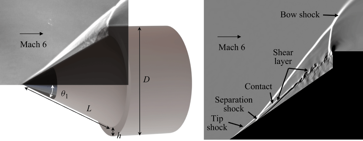
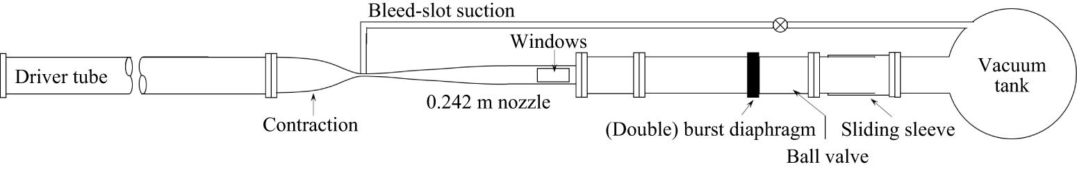
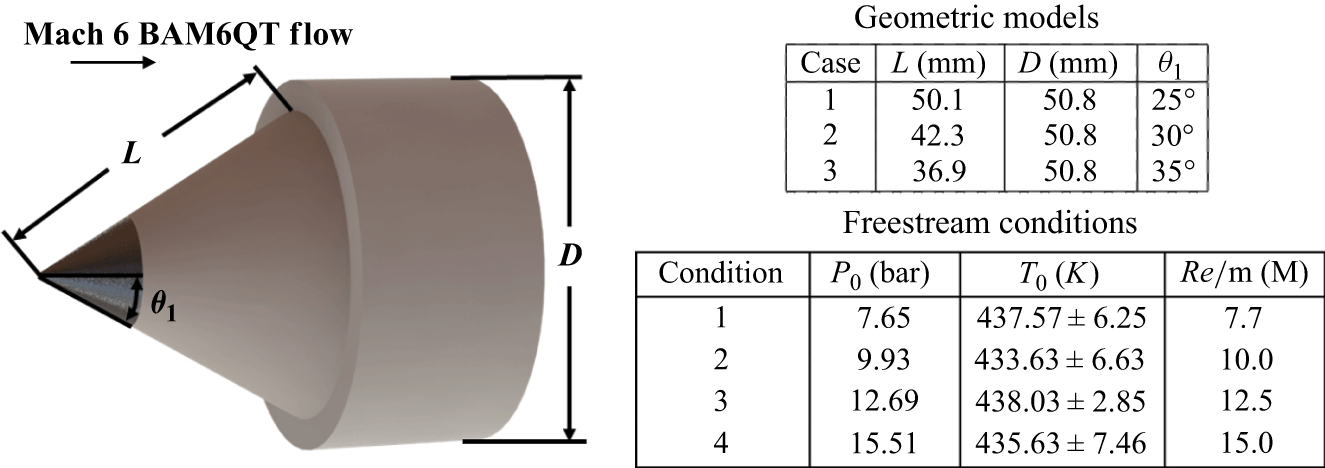
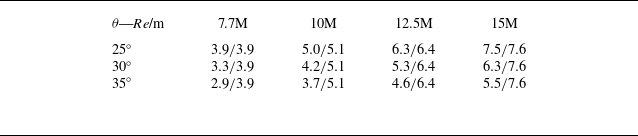


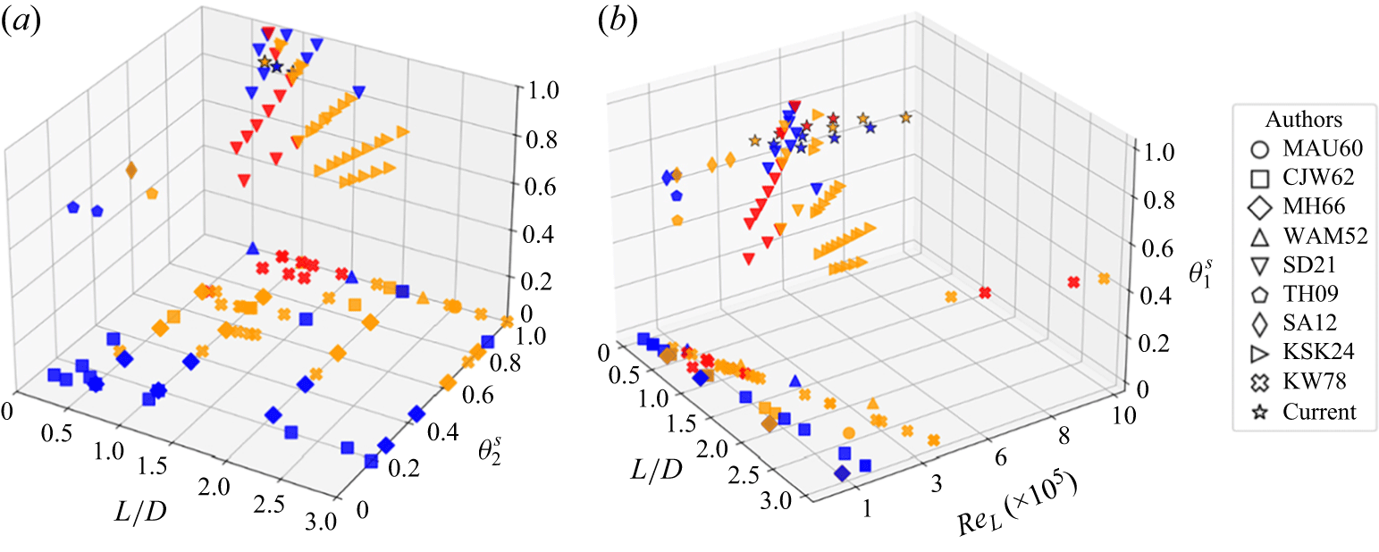


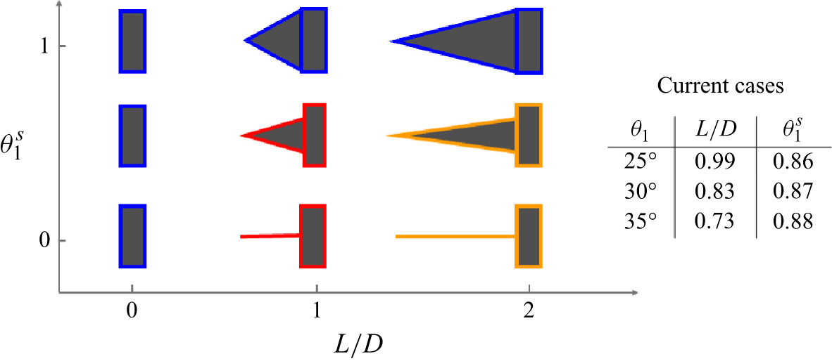


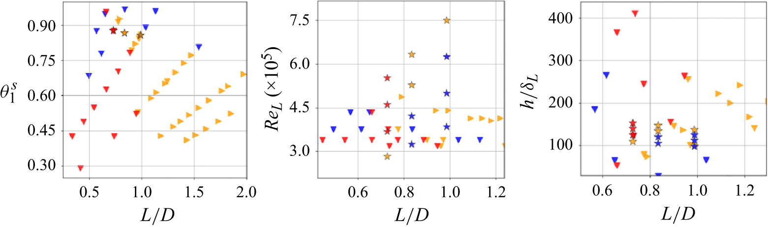


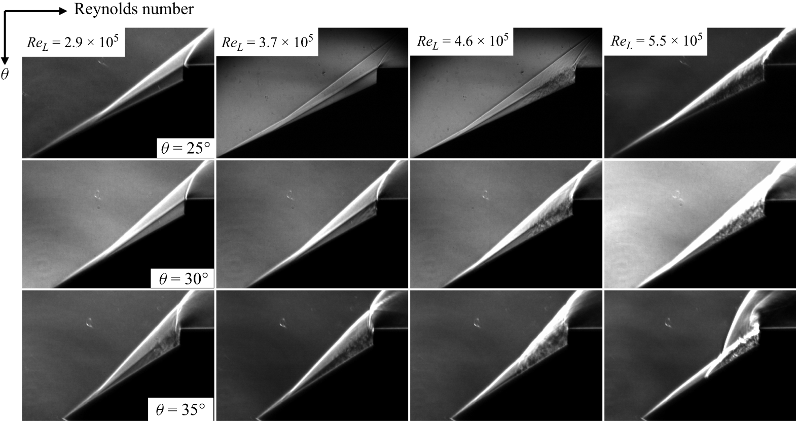

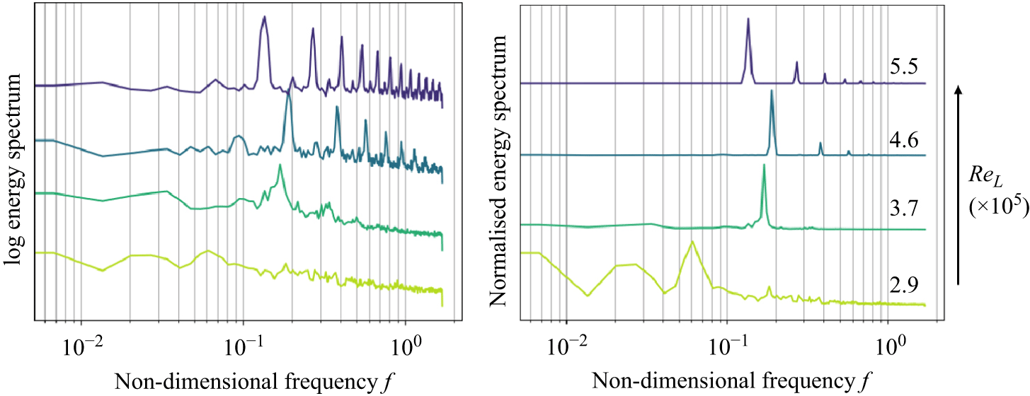


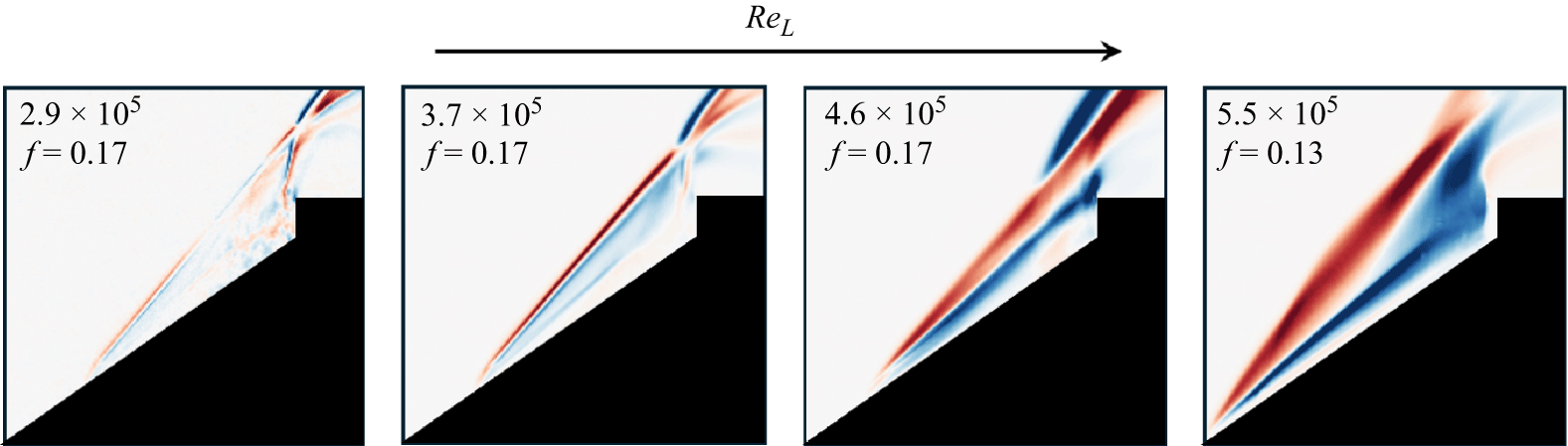


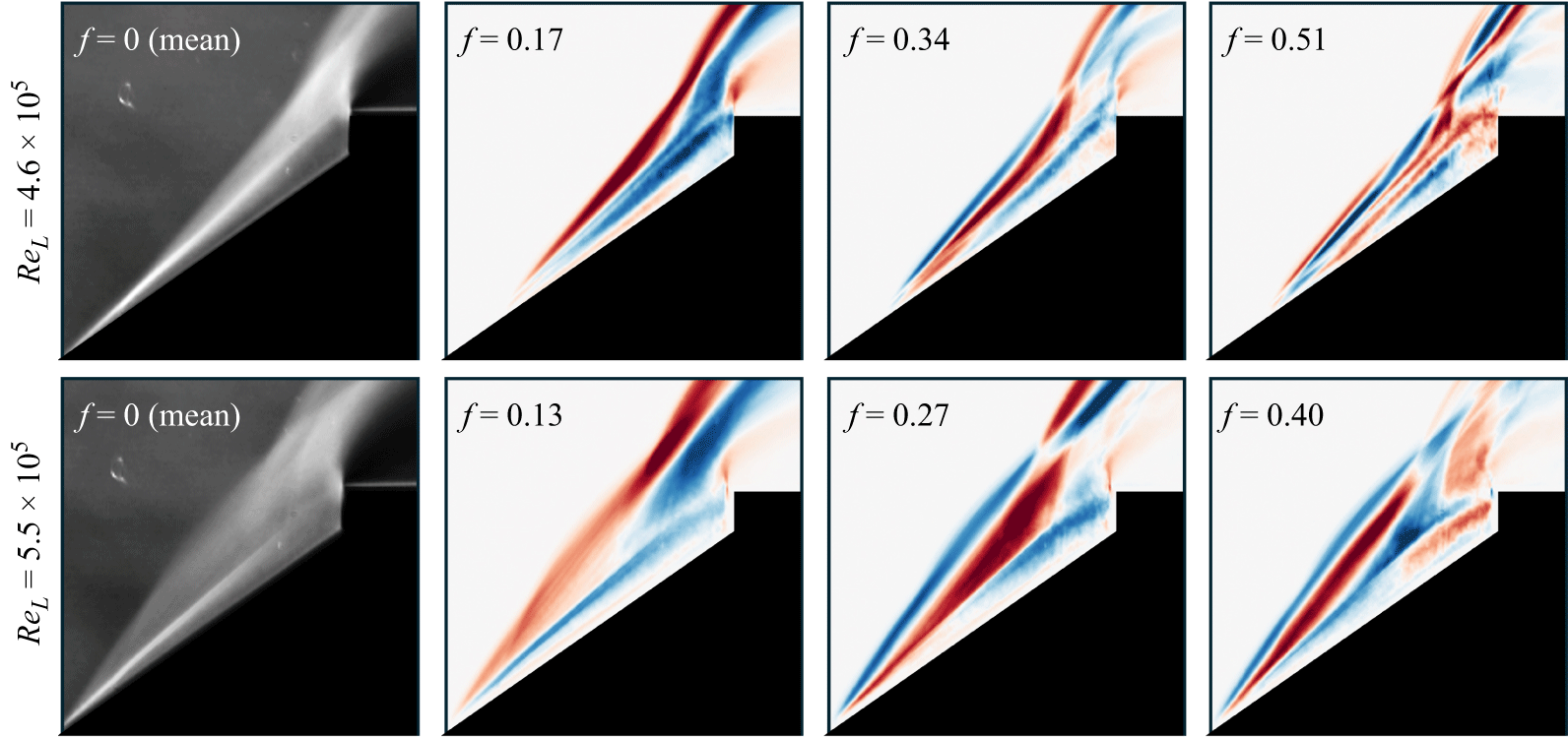


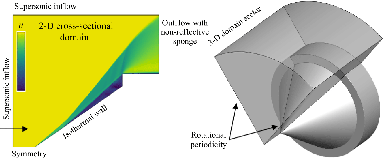
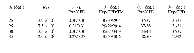

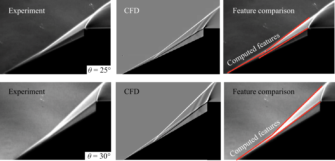


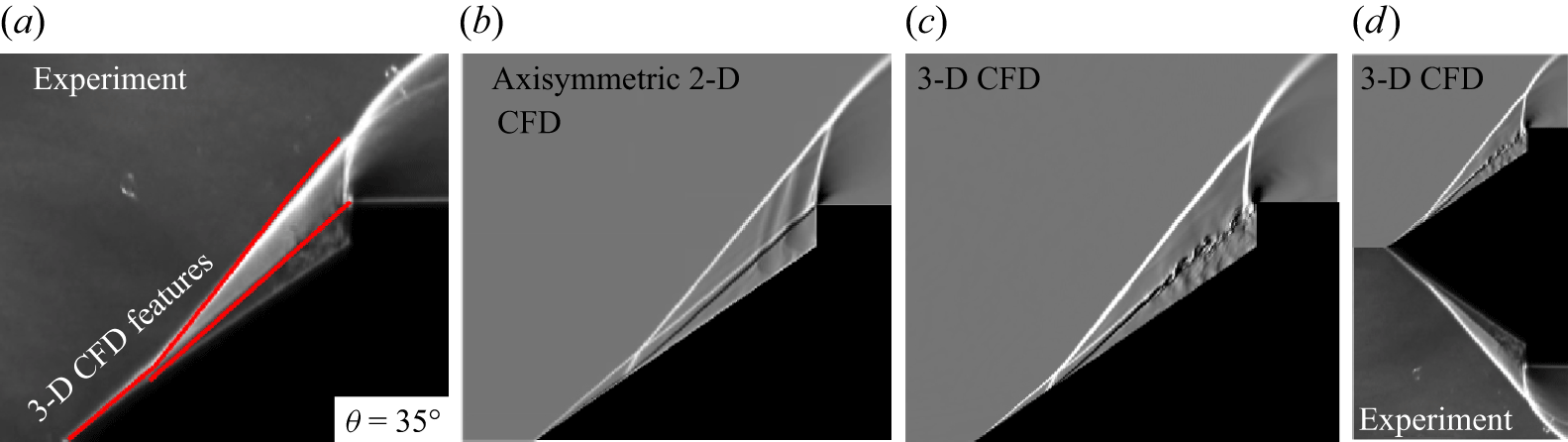


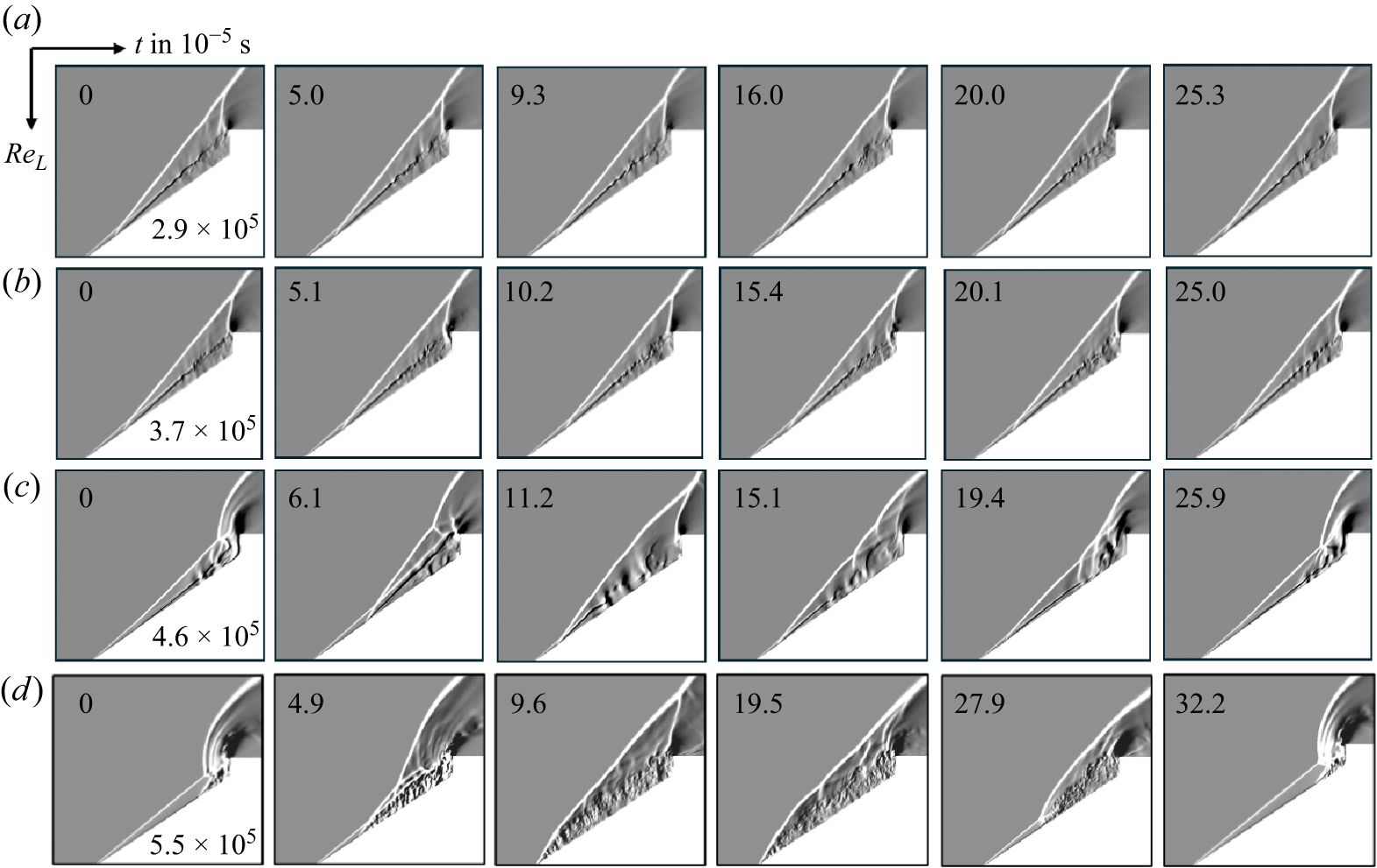


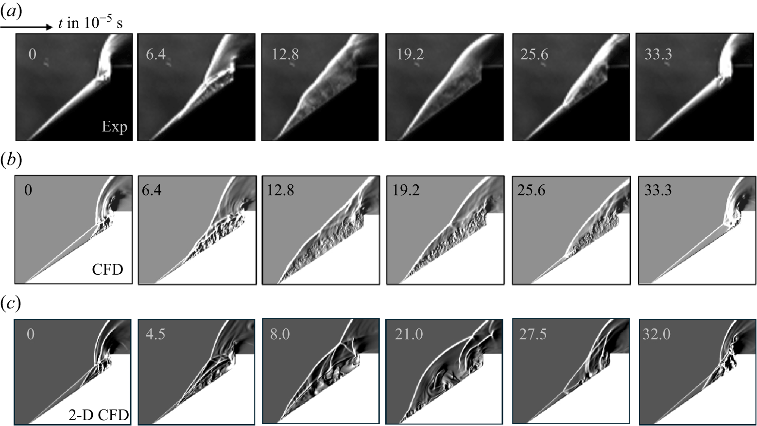


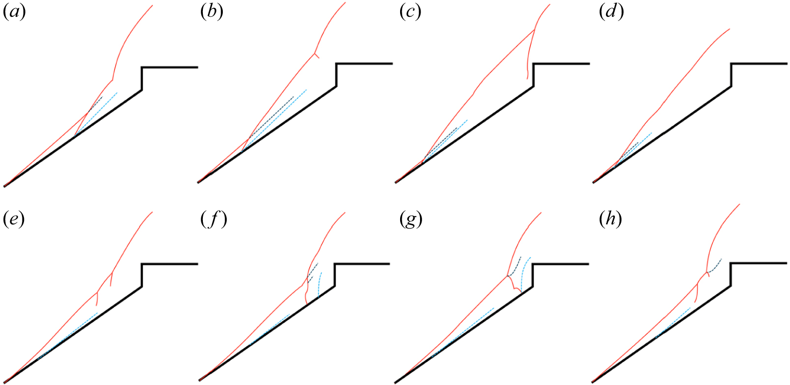


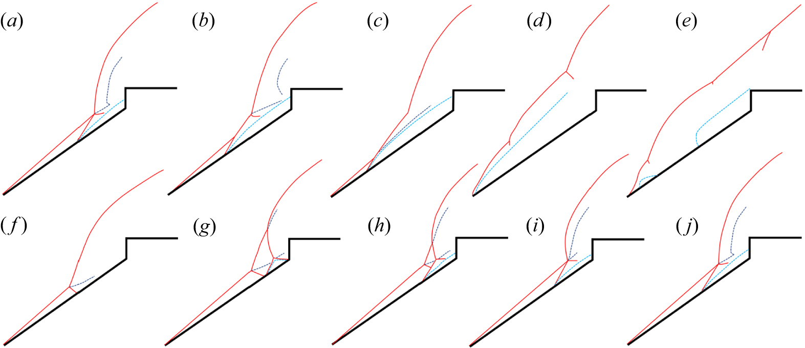


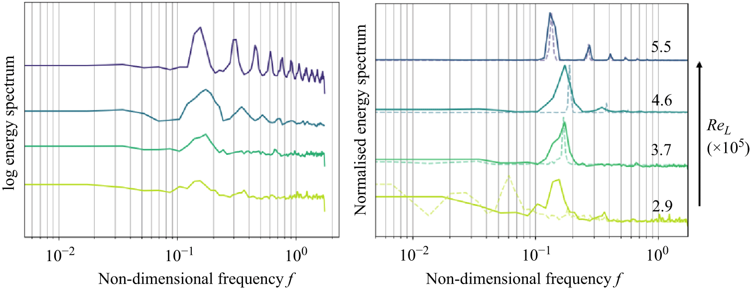

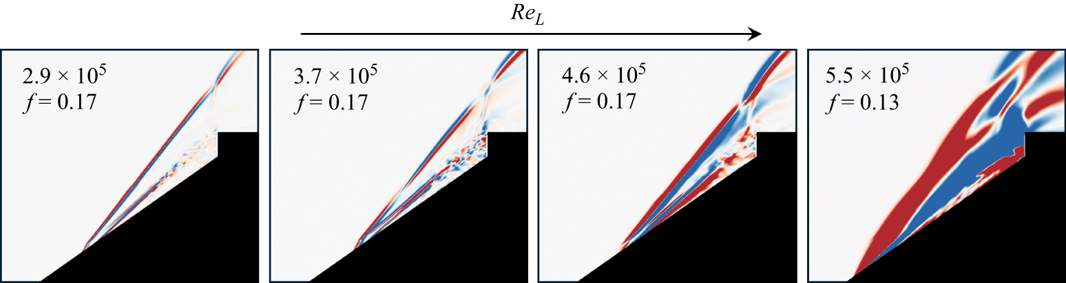

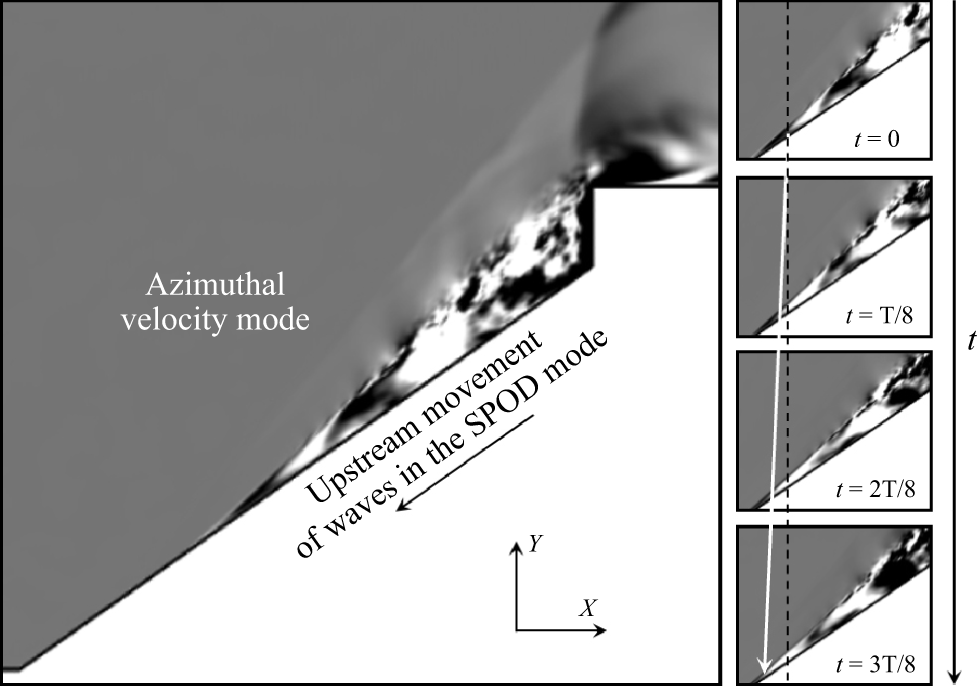


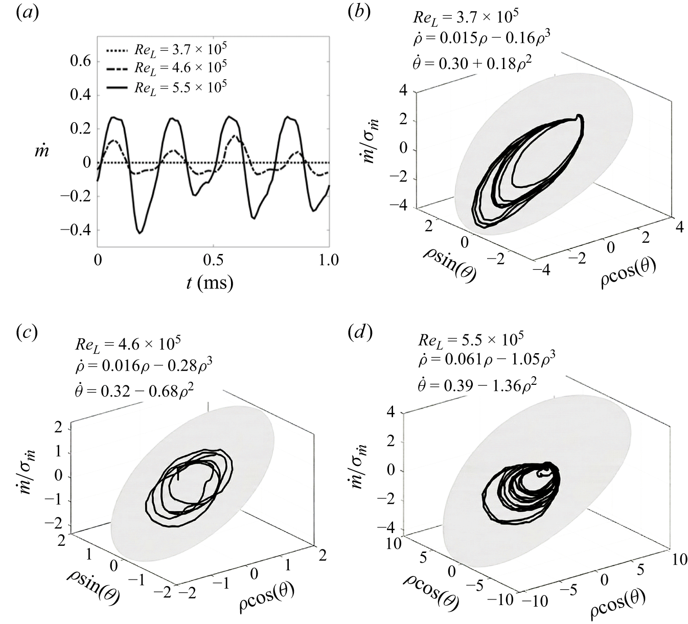


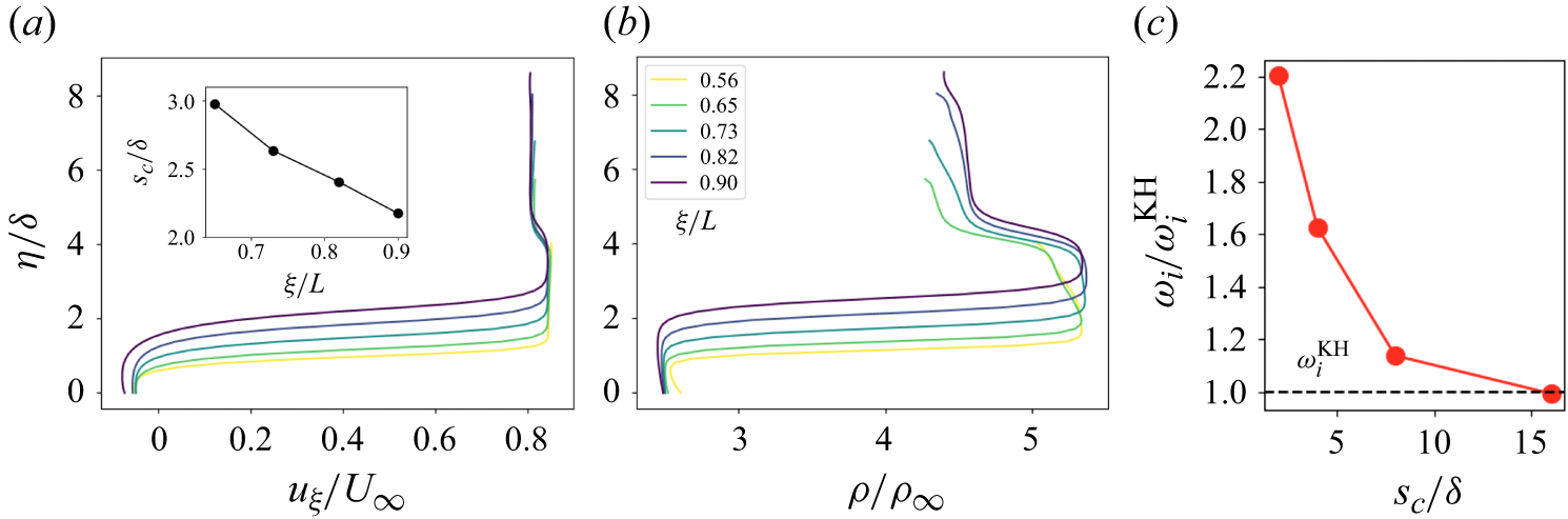


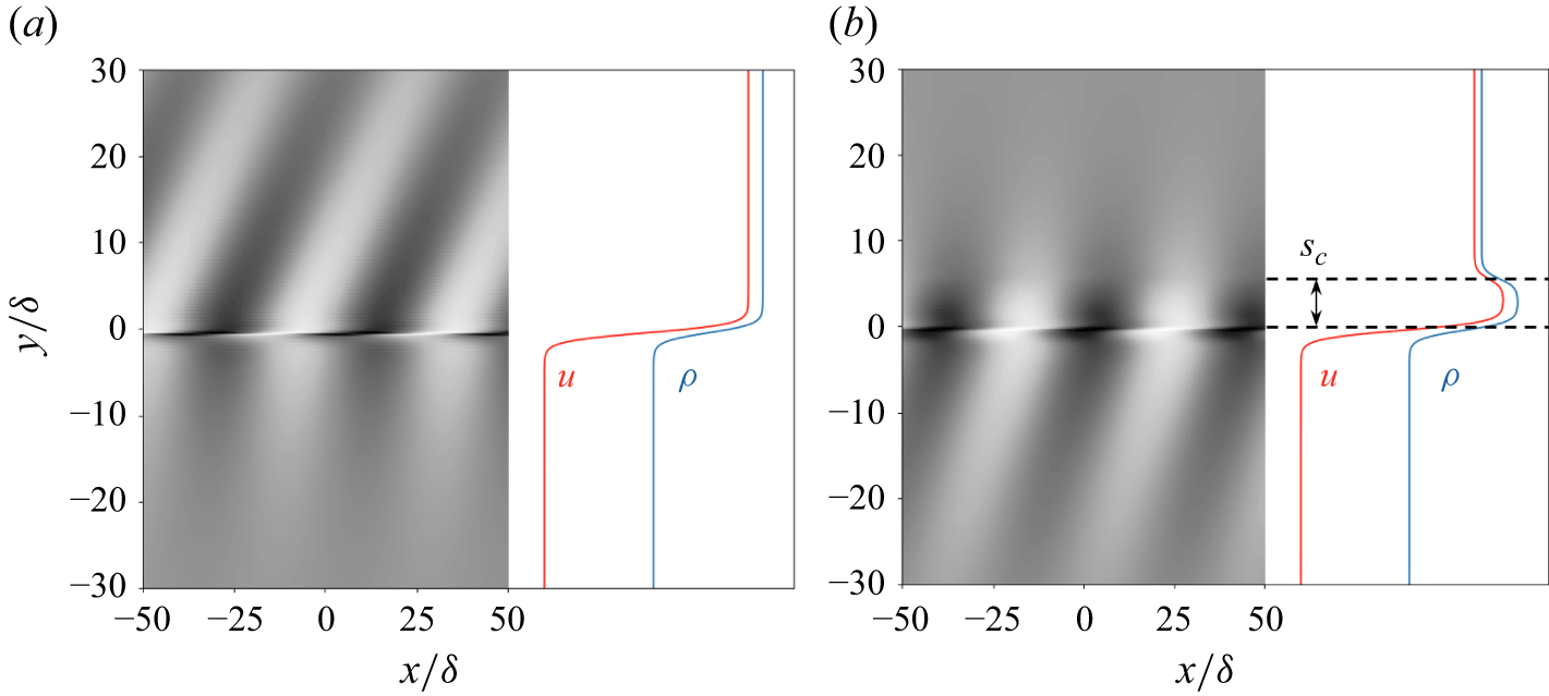

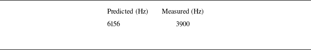


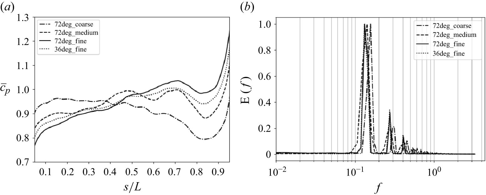


 Open access