











1 Introduction
High-intensity lasers have become indispensable tools across diverse fields, including inertial confinement fusion, laboratory astrophysics and particle acceleration[
Reference Abu-Shawareb, Acree and Adams
1
–
Reference Ziegler, Goethel, Assenbaum, Bernert, Brack, Cowan, Dover, Gaus, Kluge, Kraft, Kroll, Metzkes-Ng, Nishiuchi, Prencipe, Pueschel, Rehwald, Reimold, Schlenvoigt, Umlandt, Vescovi, Schramm and Zeil
5
]. The performance of these systems critically depends on accurate knowledge of the laser power distribution $\left(\mathrm{J}/\mathrm{s}\right)$
and fluence distribution
$\left(\mathrm{J}/\mathrm{s}\right)$
and fluence distribution $\left(\mathrm{J}/{\mathrm{cm}}^2\right)$
in focus, both of which must be properly characterized[
Reference Pirozhkov, Fukuda, Nishiuchi, Kiriyama, Sagisaka, Ogura, Mori, Kishimoto, Sakaki, Dover, Kondo, Nakanii, Huang, Kanasaki, Kondo and Kando
6
, Reference Yoon, Kim, Choi, Sung, Lee, Lee and Nam
7
]. These laser parameters are essential for proper experiment interpretation by laser–plasma experimentalists and theoreticians, a point we examine in greater detail in Section 5. Pirozhkov et al.
[
Reference Pirozhkov, Fukuda, Nishiuchi, Kiriyama, Sagisaka, Ogura, Mori, Kishimoto, Sakaki, Dover, Kondo, Nakanii, Huang, Kanasaki, Kondo and Kando
6
] explain that precise measurement of the power and fluence distributions of high-power lasers is not a simple task and common mistakes need to be avoided to accurately determine the intensity distribution at the focus position. The laser should be operated at full power and the output beam should be attenuated by wavefront preserving optics. The day-to-day and long-term reproducibility of the beamline should be taken into account. The spatio-temporal coupling should be eliminated. The fluence distribution at the focus should be imaged by an accurately aligned, high-quality, high-numerical aperture (NA) optical system (objective lens) onto a camera with high dynamic range and sufficient pixel resolution. The whole intensity distribution should be taken into account instead of only the full width at half maximum (FWHM) when determining the peak intensity. Finally, the focal spot should not be calculated as a point spread function of wavefront data in the near-field plane. We followed these instructions within the existing constraints and characterized the fluence distribution at the focus of the photodissociation laser at the Prague Asterix Laser System (PALS) facility[
Reference Jungwirth, Cejnarova, Juha, Kralikova, Krasa, Krousky, Krupickova, Laska, Masek, Mocek, Pfeifer, Präg, Renner, Rohlena, Rus, Skala, Straka and Ullschmied
8
].
$\left(\mathrm{J}/{\mathrm{cm}}^2\right)$
in focus, both of which must be properly characterized[
Reference Pirozhkov, Fukuda, Nishiuchi, Kiriyama, Sagisaka, Ogura, Mori, Kishimoto, Sakaki, Dover, Kondo, Nakanii, Huang, Kanasaki, Kondo and Kando
6
, Reference Yoon, Kim, Choi, Sung, Lee, Lee and Nam
7
]. These laser parameters are essential for proper experiment interpretation by laser–plasma experimentalists and theoreticians, a point we examine in greater detail in Section 5. Pirozhkov et al.
[
Reference Pirozhkov, Fukuda, Nishiuchi, Kiriyama, Sagisaka, Ogura, Mori, Kishimoto, Sakaki, Dover, Kondo, Nakanii, Huang, Kanasaki, Kondo and Kando
6
] explain that precise measurement of the power and fluence distributions of high-power lasers is not a simple task and common mistakes need to be avoided to accurately determine the intensity distribution at the focus position. The laser should be operated at full power and the output beam should be attenuated by wavefront preserving optics. The day-to-day and long-term reproducibility of the beamline should be taken into account. The spatio-temporal coupling should be eliminated. The fluence distribution at the focus should be imaged by an accurately aligned, high-quality, high-numerical aperture (NA) optical system (objective lens) onto a camera with high dynamic range and sufficient pixel resolution. The whole intensity distribution should be taken into account instead of only the full width at half maximum (FWHM) when determining the peak intensity. Finally, the focal spot should not be calculated as a point spread function of wavefront data in the near-field plane. We followed these instructions within the existing constraints and characterized the fluence distribution at the focus of the photodissociation laser at the Prague Asterix Laser System (PALS) facility[
Reference Jungwirth, Cejnarova, Juha, Kralikova, Krasa, Krousky, Krupickova, Laska, Masek, Mocek, Pfeifer, Präg, Renner, Rohlena, Rus, Skala, Straka and Ullschmied
8
].
Another laser beam parameter that should be monitored is the beam wavefront (phase distribution), which has a large effect on the fluence distribution in the focus. Wavefront aberrations expand the size of the focused beam and therefore significantly reduce the peak fluence. Consequently, wavefront characterization at high-power laser facilities is a crucial aspect of beam diagnostics and is often performed using Shack–Hartmann wavefront sensors[
Reference Wang, Liu, He, Pan, Zhou, Wu and Zhu
9
–
Reference Keitel, Ploenjes, Kreis, Kuhlmann, Tiedtke, Mey, Schaefer and Mann
11
]. These devices usually have phase pixel size higher than 20 μm and an angle of acceptance of around 12° ( $\mathrm{NA}\approx 0.2$
). They are unsuitable for direct measurements of f/2 focused laser beams (NA = 0.25) without additional imaging optics, which can affect the measured wavefront. However, there is a commercial wavefront sensor[
12
] with an angle of acceptance of 53° (
$\mathrm{NA}\approx 0.2$
). They are unsuitable for direct measurements of f/2 focused laser beams (NA = 0.25) without additional imaging optics, which can affect the measured wavefront. However, there is a commercial wavefront sensor[
12
] with an angle of acceptance of 53° ( $\mathrm{NA}=0.8$
) that can be used to measure the f/2 focused laser beam, but it was not at our disposal at the time of study. It is important to emphasize that characterizing the wavefront of the focused beam provides a more comprehensive analysis than measuring the collimated-beam wavefront. This approach captures additional aberrations introduced by the focusing optics, such as those resulting from manufacturing imperfections or slight misalignment.
$\mathrm{NA}=0.8$
) that can be used to measure the f/2 focused laser beam, but it was not at our disposal at the time of study. It is important to emphasize that characterizing the wavefront of the focused beam provides a more comprehensive analysis than measuring the collimated-beam wavefront. This approach captures additional aberrations introduced by the focusing optics, such as those resulting from manufacturing imperfections or slight misalignment.
Another wavefront characterization technique is phase retrieval based on the Gerchberg–Saxton algorithm[
Reference Gerchberg and Saxton
13
, Reference Wang, Song, Wang, Ren, Zhao, Dou, Di, Barbastathis, Zhou, Zhao and Lam
14
]. This method utilizes measurements of fluence distributions at different $z$
positions around the focus. The fluence measurements are then linked through Fresnel propagation in multi-plane phase retrieval[
Reference Allen and Oxley
15
]. Complex amplitudes (electric intensity and wavefront) are iteratively propagated between fluence measurements at different
$z$
positions around the focus. The fluence measurements are then linked through Fresnel propagation in multi-plane phase retrieval[
Reference Allen and Oxley
15
]. Complex amplitudes (electric intensity and wavefront) are iteratively propagated between fluence measurements at different $z$
positions, which eventually leads to phase extraction. Phase retrieval is an active research area, and there are several ways to improve the speed and accuracy of the algorithm. For example, unordered steps can be applied in the iteration cycle[
Reference Binamira and Almoro
16
], or more sophisticated combinations of measured and propagated electric field amplitudes can be used[
Reference Brady and Fienup
17
–
Reference Chalupsky, Bohacek, Burian, Hajkova, Hau-Riege, Heimann, Juha, Messerschmidt, Moeller, Nagler, Rowen, Schlotter, Swiggers, Turner and Krzywinski
19
]. The phase retrieval approach is of significant interest in the high-power laser community because it can easily and accurately characterize laser caustics and phase aberrations[
Reference Bahk, Bromage, Begishev, Mileham, Stoeckl, Storm and Zuegel
20
–
Reference Wang, Ghazagh, Ravi, Baumbach, Dannecker, Scharun, Bauer, Nolte and Flamm
23
].
$z$
positions, which eventually leads to phase extraction. Phase retrieval is an active research area, and there are several ways to improve the speed and accuracy of the algorithm. For example, unordered steps can be applied in the iteration cycle[
Reference Binamira and Almoro
16
], or more sophisticated combinations of measured and propagated electric field amplitudes can be used[
Reference Brady and Fienup
17
–
Reference Chalupsky, Bohacek, Burian, Hajkova, Hau-Riege, Heimann, Juha, Messerschmidt, Moeller, Nagler, Rowen, Schlotter, Swiggers, Turner and Krzywinski
19
]. The phase retrieval approach is of significant interest in the high-power laser community because it can easily and accurately characterize laser caustics and phase aberrations[
Reference Bahk, Bromage, Begishev, Mileham, Stoeckl, Storm and Zuegel
20
–
Reference Wang, Ghazagh, Ravi, Baumbach, Dannecker, Scharun, Bauer, Nolte and Flamm
23
].
In this paper, we present the characterization of intensity distributions and beam wavefronts along the caustic of the iodine photodissociation laser at the PALS facility. We measured fluence distributions by far-field imaging using a camera corrected for nonlinearities by a nonlinear response function recovery (NoReFry) algorithm[
Reference Vozda, Burian, Hájková, Juha, Enkisch, Faatz, Hermann, Jacyna, Jurek, Keitel, Klinger, Loch, Louis, Makhotkin, Plönjes, Saksl, Siewert, Sobierajski, Strobel, Tiedtke, Toleikis, de Vries, Zelinger and Chalupský
24
]. We then retrieved the beam wavefront using a phase retrieval algorithm and propagated the wavefront along the caustic and back to the lens position[
Reference Brady and Fienup
17
] to determine aberrations of the focusing lens and the collimated beam. Finally, we combined fluence and laser power distributions to obtain intensity distributions with a peak intensity above the relativistic threshold of $0.8\times {10}^{18}\;\mathrm{W}/{\mathrm{cm}}^2$
at
$0.8\times {10}^{18}\;\mathrm{W}/{\mathrm{cm}}^2$
at $1315.2\;\mathrm{nm}$
[
Reference Mourou, Chang, Maksimchuk, Nees, Bulanov, Bychenkov, Esirkepov, Naumova, Pegoraro and Ruhl
25
].
$1315.2\;\mathrm{nm}$
[
Reference Mourou, Chang, Maksimchuk, Nees, Bulanov, Bychenkov, Esirkepov, Naumova, Pegoraro and Ruhl
25
].
2 Experimental setup
2.1 Standard PALS laser setup
The high-power iodine photodissociation laser system at the PALS facility operates at the fundamental wavelength $\lambda =1315.2\;\mathrm{nm}$
with bandwidth 170 pm and delivers laser pulses with energies up to approximately
$\lambda =1315.2\;\mathrm{nm}$
with bandwidth 170 pm and delivers laser pulses with energies up to approximately $700\;\mathrm{J}$
and duration
$700\;\mathrm{J}$
and duration ${\tau}_{\mathrm{FWHM}}\sim 300\;\mathrm{ps}$
[
Reference Jungwirth, Cejnarova, Juha, Kralikova, Krasa, Krousky, Krupickova, Laska, Masek, Mocek, Pfeifer, Präg, Renner, Rohlena, Rus, Skala, Straka and Ullschmied
8
].
${\tau}_{\mathrm{FWHM}}\sim 300\;\mathrm{ps}$
[
Reference Jungwirth, Cejnarova, Juha, Kralikova, Krasa, Krousky, Krupickova, Laska, Masek, Mocek, Pfeifer, Präg, Renner, Rohlena, Rus, Skala, Straka and Ullschmied
8
].
The laser pulse is extracted from a pulse train sequence generated by a mode-locked oscillator. It is then amplified by five flashlamp-pumped laser amplifiers, resulting in a flat-top fluence distribution at the output. To eliminate high spatial frequencies in the fluence distribution, six vacuum spatial filters are used; these filters transfer the beam between each pair of adjacent laser amplifiers, with the final spatial filter transferring the beam from the last amplifier to a focusing lens in the target chamber. The laser system layout is shown in Figure 1.
Schematic layout of the iodine photodissociation laser at the Prague Asterix Laser System facility. The oscillator and preamplifier part is simplified. The image is adapted with permission from Ref. [Reference Dostal, Dudzak, Pisarczyk, Pfeifer, Huynh, Chodukowski, Kalinowska, Krousky, Skala, Hrebicek, Medrik, Golasowski, Juha and Ullschmied26].

The output laser beam with a diameter of 290 mm is focused by an $f/2.2$
aspherical focusing lens with focal length
$f/2.2$
aspherical focusing lens with focal length $f=627\;\mathrm{mm}$
at
$f=627\;\mathrm{mm}$
at $\lambda =1315.2\;\mathrm{nm}$
. The lens is designed to create a diffraction-limited focus with focal length
$\lambda =1315.2\;\mathrm{nm}$
. The lens is designed to create a diffraction-limited focus with focal length $f=600\;\mathrm{mm}$
at
$f=600\;\mathrm{mm}$
at $\lambda =438\;\mathrm{nm}$
(third harmonic) in the geometrical optics approximation. Therefore, we expect aberrations at
$\lambda =438\;\mathrm{nm}$
(third harmonic) in the geometrical optics approximation. Therefore, we expect aberrations at $\lambda =1315.2\;\mathrm{nm}$
, specifically the spherical aberration. During the experiment, we did not have a lens corrected for 1315.2 nm at our disposal.
$\lambda =1315.2\;\mathrm{nm}$
, specifically the spherical aberration. During the experiment, we did not have a lens corrected for 1315.2 nm at our disposal.
We determine the focus position experimentally by inserting a metal Hartmann plate into the collimated beam immediately upstream of the lens. The Hartmann plate cuts out five beams ( $\mathrm{\unicode{xf8}}=20\;\mathrm{mm}$
) located on a circle perimeter (
$\mathrm{\unicode{xf8}}=20\;\mathrm{mm}$
) located on a circle perimeter ( $\mathrm{\unicode{xf8}}=200\;\mathrm{mm}$
) around the center of the main beam. We conduct a series of four laser shots on an aluminum target at the target chamber center (TCC). For each shot, the focusing lens is positioned at different distances (
$\mathrm{\unicode{xf8}}=200\;\mathrm{mm}$
) around the center of the main beam. We conduct a series of four laser shots on an aluminum target at the target chamber center (TCC). For each shot, the focusing lens is positioned at different distances ( $-$
6,
$-$
6, $-$
3, 3 and 6 mm) relative to the expected focus position. We capture microscope images of the resulting ablation patterns, where each pattern contains five holes corresponding to the five beams, and we measure the distances between the centers of the leftmost and rightmost craters. We plot the measured distances (negative when the ablated pattern is inverted through the center) against the focusing lens positions and perform a linear fit. Its intersection point with the
$-$
3, 3 and 6 mm) relative to the expected focus position. We capture microscope images of the resulting ablation patterns, where each pattern contains five holes corresponding to the five beams, and we measure the distances between the centers of the leftmost and rightmost craters. We plot the measured distances (negative when the ablated pattern is inverted through the center) against the focusing lens positions and perform a linear fit. Its intersection point with the $z$
-position axis determines the focus position.
$z$
-position axis determines the focus position.
Beam parameters are monitored online using an attenuated part of the laser beam that is transmitted through a high-reflectivity mirror after the last laser amplifier. The attenuated laser pulse is split and measured by diagnostic devices. A calibrated calorimeter measures the pulse energy. Four photodiodes with different trigger timings and different attenuation filters in front of them measure the laser pulse power distribution in the prepulse before the main laser peak. Together, the photodiodes measure the power distribution in the range of 10 ns before and 0.8 ns after the main laser peak. The highest power peak of the laser pulse is measured by a streak camera. A slit of width 30 μm cuts out a rectangle from the laser beam, which irradiates a photocathode and the emitted electrons are streaked in time. We join the normalized power distributions measured by the photodiodes and the streak camera at $0.05\times$
the peak power to characterize the entire power distribution.
$0.05\times$
the peak power to characterize the entire power distribution.
2.2 Measuring the fluence distribution at and around the focus position
We measure the fluence distribution in multiple planes at and around the focus position in the target chamber by far-field imaging (i.e., projecting a magnified image of the fluence distribution onto a camera). Firstly, we build the imaging setup (Figure 2) and determine its magnification factor. We place a calibration target (grid with 10 μm spacing) at the TCC, illuminate it with a defocused alignment neodymium-doped yttrium lithium fluoride (Nd:YLF) laser beam (CrystalLaser IRCL-1W-1313, $\lambda =1313\;\mathrm{nm}$
) and project the grid’s magnified image onto a near-infrared charge-coupled device (CCD) camera (Goldeye G-032 SWIR TEC, 25 μm pixel size, number of pixels
$\lambda =1313\;\mathrm{nm}$
) and project the grid’s magnified image onto a near-infrared charge-coupled device (CCD) camera (Goldeye G-032 SWIR TEC, 25 μm pixel size, number of pixels $636\times 508$
) using a microscope objective without a tube lens (
$636\times 508$
) using a microscope objective without a tube lens ( $50$
× Mitutoyo Plan Apochromatic Infinity Corrected Long Working Distance Objective,
$50$
× Mitutoyo Plan Apochromatic Infinity Corrected Long Working Distance Objective, $f=4\;\mathrm{mm}$
,
$f=4\;\mathrm{mm}$
, $\mathrm{NA}=0.55,\ f\text{-}\mathrm{number}\approxeq 0.9$
, corrected for visible wavelengths
$\mathrm{NA}=0.55,\ f\text{-}\mathrm{number}\approxeq 0.9$
, corrected for visible wavelengths $\approx 400$
–700 nm). The microscope objective is corrected for imaging of visible light into infinity. Although we used the near-infrared wavelength of (
$\approx 400$
–700 nm). The microscope objective is corrected for imaging of visible light into infinity. Although we used the near-infrared wavelength of ( $1315.2\pm 0.1$
) nm and the image distance was 340 mm, the calibration grid was imaged with high quality without significant aberrations. We measured the edge-spread function of the imaging system and determined that the modulation transfer function at 10% contrast is reached for spatial frequency at 500 line pairs per mm (
$1315.2\pm 0.1$
) nm and the image distance was 340 mm, the calibration grid was imaged with high quality without significant aberrations. We measured the edge-spread function of the imaging system and determined that the modulation transfer function at 10% contrast is reached for spatial frequency at 500 line pairs per mm ( $\mathrm{MTF}10=500\;\mathrm{lp}/\mathrm{mm}$
)[
Reference Boreman
27
, Reference Smith
28
]. This was made possible by the narrow bandwidth that minimized the potential chromatic aberration, good alignment of the objective and small beam filling factor of the entrance lens that reduced the spherical and other aberrations. After determining the magnification factor of 84 and the scale of
$\mathrm{MTF}10=500\;\mathrm{lp}/\mathrm{mm}$
)[
Reference Boreman
27
, Reference Smith
28
]. This was made possible by the narrow bandwidth that minimized the potential chromatic aberration, good alignment of the objective and small beam filling factor of the entrance lens that reduced the spherical and other aberrations. After determining the magnification factor of 84 and the scale of $0.3\;\mu \mathrm{m}/\mathrm{px}$
, we focus the alignment laser beam at the TCC and insert large-diameter (
$0.3\;\mu \mathrm{m}/\mathrm{px}$
, we focus the alignment laser beam at the TCC and insert large-diameter ( $\mathrm{\unicode{xf8}}=340\;\mathrm{mm}$
) neutral-density optical filters into its collimated-beam path (upstream of the focusing lens) to check that they do not visibly change the far-field. The alignment laser beam diameter at these optical filters is 290 mm, the same as for the iodine laser. When all seven large optical filters are inserted, they attenuate the fully amplified iodine laser pulse from
$\mathrm{\unicode{xf8}}=340\;\mathrm{mm}$
) neutral-density optical filters into its collimated-beam path (upstream of the focusing lens) to check that they do not visibly change the far-field. The alignment laser beam diameter at these optical filters is 290 mm, the same as for the iodine laser. When all seven large optical filters are inserted, they attenuate the fully amplified iodine laser pulse from $700\;\mathrm{J}$
down to approximately
$700\;\mathrm{J}$
down to approximately $1\;\mathrm{mJ}$
. The pulse then passes through the focusing lens, and the fluence distribution at the TCC is magnified and imaged onto the camera, all in air. We decrease the laser pulse energy so we do not ignite a spark in air with the focused laser beam. We insert small neutral-density
$1\;\mathrm{mJ}$
. The pulse then passes through the focusing lens, and the fluence distribution at the TCC is magnified and imaged onto the camera, all in air. We decrease the laser pulse energy so we do not ignite a spark in air with the focused laser beam. We insert small neutral-density $50$
mm
$\times$
$50$
mm square filters (Hoya) in front of the camera to further attenuate the beam and stay below the camera saturation limit. We translate the focusing lens along the
$50$
mm
$\times$
$50$
mm square filters (Hoya) in front of the camera to further attenuate the beam and stay below the camera saturation limit. We translate the focusing lens along the $z$
-axis (beam propagation direction) between the shots to create a
$z$
-axis (beam propagation direction) between the shots to create a $z$
-scan of fluence distributions along the beam caustic.
$z$
-scan of fluence distributions along the beam caustic.
Diagram of the setup for fluence distribution measurements along the beam caustic. We shift the focusing lens within a range of $\pm$
300 μm around the expected best focus position to perform the
$\pm$
300 μm around the expected best focus position to perform the $z$
-scan. Distances among the object plane, the front principal plane of the microscope objective and the camera are calculated based on the magnification of the calibration target (84×).
$z$
-scan. Distances among the object plane, the front principal plane of the microscope objective and the camera are calculated based on the magnification of the calibration target (84×).

3 Analysis methods
3.1 Retrieving the complex amplitude from the measured fluence distributions
We retrieved complete information about the complex amplitude of the electric field from several fluence distribution measurements at different $z$
positions along the beam propagation direction. Subsequently, we propagated the beam throughout its caustic.
$z$
positions along the beam propagation direction. Subsequently, we propagated the beam throughout its caustic.
Phase retrieval approaches can extract phase from a set of fluence distribution measurements. We used a multi-plane phase retrieval algorithm with dynamic input–output mixing (PhaRe)[ Reference Chalupsky, Bohacek, Burian, Hajkova, Hau-Riege, Heimann, Juha, Messerschmidt, Moeller, Nagler, Rowen, Schlotter, Swiggers, Turner and Krzywinski 19 ] using functions adapted from the LightPipes library for Python[ 29 ]. The main idea is illustrated in Figure 3.
Illustrative flowchart of the jth iteration loop of PhaRe applied to three fluence distribution measurements. The illustrative iteration starts at the position ${z}_1$
, but the final retrieved complex amplitude is independent of the starting position. Green circles represent the measured electric field amplitudes
${z}_1$
, but the final retrieved complex amplitude is independent of the starting position. Green circles represent the measured electric field amplitudes $\left|{E}_n^{\mathrm{M}}\right|$
, yellow rectangles represent the complex amplitudes
$\left|{E}_n^{\mathrm{M}}\right|$
, yellow rectangles represent the complex amplitudes $\left|{E}_n^{\mathrm{P}}\right|\exp \left(i{\varphi}_n\right)$
propagated from the previous
$\left|{E}_n^{\mathrm{P}}\right|\exp \left(i{\varphi}_n\right)$
propagated from the previous $z$
position and blue rectangles represent the temporary retrieved complex amplitudes
$z$
position and blue rectangles represent the temporary retrieved complex amplitudes $\left|{E}_n\right|\exp \left(i{\varphi}_n\right)$
. The temporary retrieved electric field amplitude is calculated as a linear combination of the corresponding measured and propagated electric field amplitudes
$\left|{E}_n\right|\exp \left(i{\varphi}_n\right)$
. The temporary retrieved electric field amplitude is calculated as a linear combination of the corresponding measured and propagated electric field amplitudes ${\alpha}_j\left|{E}_n^{\mathrm{M}}\right|+{\beta}_j\left|{E}_n^{\mathrm{P}}\right|$
. The forward and backward propagation steps are highlighted in blue and red colors, respectively. The black arrows represent copying of the complex amplitude. The image is adapted with permission from Ref. [Reference Chalupsky, Bohacek, Burian, Hajkova, Hau-Riege, Heimann, Juha, Messerschmidt, Moeller, Nagler, Rowen, Schlotter, Swiggers, Turner and Krzywinski19], copyright 2015, American Physical Society.
${\alpha}_j\left|{E}_n^{\mathrm{M}}\right|+{\beta}_j\left|{E}_n^{\mathrm{P}}\right|$
. The forward and backward propagation steps are highlighted in blue and red colors, respectively. The black arrows represent copying of the complex amplitude. The image is adapted with permission from Ref. [Reference Chalupsky, Bohacek, Burian, Hajkova, Hau-Riege, Heimann, Juha, Messerschmidt, Moeller, Nagler, Rowen, Schlotter, Swiggers, Turner and Krzywinski19], copyright 2015, American Physical Society.

Firstly, we preprocess each of the total number of $N$
input fluence distributions measured at
$N$
input fluence distributions measured at ${z}_n$
positions (
${z}_n$
positions ( $n\in \left\{0,1,\dots, N-1\right\}$
). We use ImageJ software to subtract the dark image (the laser, amplifier flashlamps and lights are off) and then the mean of the background. We set any negative-value pixels to zero since those pixels do not carry information about the signal. The residual background remaining after the dark image subtraction is caused by broadband radiation from the flashlamps that pump the last laser amplifier. A small part of this incoherent radiation propagates into the experimental chamber and onto the camera, where it is measured as shot-to-shot-variable background. After background subtraction, we manually select the non-irradiated region, where we set the signal to zero. In Python, we smooth each image using a median filter
$n\in \left\{0,1,\dots, N-1\right\}$
). We use ImageJ software to subtract the dark image (the laser, amplifier flashlamps and lights are off) and then the mean of the background. We set any negative-value pixels to zero since those pixels do not carry information about the signal. The residual background remaining after the dark image subtraction is caused by broadband radiation from the flashlamps that pump the last laser amplifier. A small part of this incoherent radiation propagates into the experimental chamber and onto the camera, where it is measured as shot-to-shot-variable background. After background subtraction, we manually select the non-irradiated region, where we set the signal to zero. In Python, we smooth each image using a median filter $5\times 5$
and correct the measured nonlinear signal using a calibration function (described in Section 3.5). We insert the image into a larger array filled with zeros and shift the beam centroid to the center to ensure that beam momentum is conserved. To meet the condition of pulse energy conservation when propagating the beam in free space, we normalize each fluence distribution by dividing by pulse energy. We calculate the pulse energy using Equation (6) by multiplying the peak value of the fluence distribution with the effective area. Another possibility is to use the measured pulse energy from the on-shot diagnostic. We address the different normalizations in Section 5.1. Finally, we take square roots of the normalized fluence distributions, which are proportional to the measured (superscript M) electric field amplitudes
$5\times 5$
and correct the measured nonlinear signal using a calibration function (described in Section 3.5). We insert the image into a larger array filled with zeros and shift the beam centroid to the center to ensure that beam momentum is conserved. To meet the condition of pulse energy conservation when propagating the beam in free space, we normalize each fluence distribution by dividing by pulse energy. We calculate the pulse energy using Equation (6) by multiplying the peak value of the fluence distribution with the effective area. Another possibility is to use the measured pulse energy from the on-shot diagnostic. We address the different normalizations in Section 5.1. Finally, we take square roots of the normalized fluence distributions, which are proportional to the measured (superscript M) electric field amplitudes $\left|{E}_n^{\mathrm{M}}\right|$
at positions
$\left|{E}_n^{\mathrm{M}}\right|$
at positions ${z}_n$
.
${z}_n$
.
Secondly, we iteratively propagate the complex amplitude ${E}_n\left(x,y\right)$
consisting of amplitude
${E}_n\left(x,y\right)$
consisting of amplitude $\left|{E}_n^{\mathrm{M}}\left(x,y\right)\right|$
and phase
$\left|{E}_n^{\mathrm{M}}\left(x,y\right)\right|$
and phase ${\varphi}_n\left(x,y\right)$
,
${\varphi}_n\left(x,y\right)$
,
 $$\begin{align}{E}_n\left(x,y\right)=\left|{E}_n^{\mathrm{M}}\left(x,y\right)\right|\exp \left[i{\varphi}_n\left(x,y\right)\right],\end{align}$$
to a neighboring position $m=n+1$
(forward steps) or
$m=n+1$
(forward steps) or $m=n-1$
(backward steps). The iteration cycle starts at an arbitrary position
$m=n-1$
(backward steps). The iteration cycle starts at an arbitrary position ${z}_{n_0}$
. The complex amplitude
${z}_{n_0}$
. The complex amplitude ${E}_{n_0}\left(x,y\right)$
is propagated using Equation (2) from the position
${E}_{n_0}\left(x,y\right)$
is propagated using Equation (2) from the position ${z}_{n_0}$
forward into the position
${z}_{n_0}$
forward into the position ${z}_m$
, where
${z}_m$
, where $m={n}_0+1$
. The next forward step starts at the position
$m={n}_0+1$
. The next forward step starts at the position ${z}_{n_0+1}$
and ends at the position
${z}_{n_0+1}$
and ends at the position ${z}_{n_0+2}$
. The forward steps continue until the rightmost position
${z}_{n_0+2}$
. The forward steps continue until the rightmost position ${z}_{N-1}$
is reached. This is followed by the backward steps where the complex amplitude is propagated through the positions
${z}_{N-1}$
is reached. This is followed by the backward steps where the complex amplitude is propagated through the positions ${z}_{N-2},{z}_{N-3},\dots, {z}_0$
until the leftmost position is reached. Then, the last forward steps propagate the complex amplitude through the positions
${z}_{N-2},{z}_{N-3},\dots, {z}_0$
until the leftmost position is reached. Then, the last forward steps propagate the complex amplitude through the positions ${z}_0,{z}_1,\dots, {z}_{n_0-1}$
to the starting position
${z}_0,{z}_1,\dots, {z}_{n_0-1}$
to the starting position ${z}_{n_0}$
. This marks the end of one iteration cycle and the following cycle starts at the same position
${z}_{n_0}$
. This marks the end of one iteration cycle and the following cycle starts at the same position ${z}_{n_0}$
. We propagate
${z}_{n_0}$
. We propagate ${E}_n\left(x,y\right)$
using the angular spectrum method:
${E}_n\left(x,y\right)$
using the angular spectrum method:
 $$\begin{align}{E}_m^{\mathrm{P}}\left(x,y\right)={\mathrm{\mathcal{F}}}^{-1}\left\{\mathrm{\mathcal{F}}\left[{E}_n\left(x,y\right)\right]{H}_m\left({f}_x,{f}_y\right)\right\},\end{align}$$
where the superscript P denotes that the resulting complex amplitude is a result of numerical propagation, $\mathrm{\mathcal{F}},{\mathrm{\mathcal{F}}}^{-1}$
are Fourier and inverse Fourier transforms, respectively,
$\mathrm{\mathcal{F}},{\mathrm{\mathcal{F}}}^{-1}$
are Fourier and inverse Fourier transforms, respectively, ${H}_m\left({f}_x,{f}_y\right)$
is a transfer function of free space and
${H}_m\left({f}_x,{f}_y\right)$
is a transfer function of free space and ${f}_x,\ {f}_y$
are spatial frequencies. We used the Rayleigh–Sommerfeld transfer function in Equation (2):
${f}_x,\ {f}_y$
are spatial frequencies. We used the Rayleigh–Sommerfeld transfer function in Equation (2):
 $$\begin{align}{H}_m\left({f}_x,{f}_y\right)=\left\{\begin{array}{@{}r@{}}\exp \left\{ ik{\zeta}_m\left[\sqrt{1-{\left(\lambda {f}_x\right)}^2-{\left(\lambda {f}_y\right)}^2}\right]\right\}\\[10pt]{}\kern1em \mathrm{for}\sqrt{f_x^2+{f}_y^2}<\frac{1}{\lambda},\\[6pt]{}0\kern9.12em \mathrm{otherwise},\end{array}\right.\end{align}$$
where $k=\left|\left({k}_x,{k}_y,{k}_z\right)\right|=2\pi /\lambda$
is the wavenumber (wavevector amplitude) and
$k=\left|\left({k}_x,{k}_y,{k}_z\right)\right|=2\pi /\lambda$
is the wavenumber (wavevector amplitude) and ${\zeta}_m={z}_m-{z}_n$
is the propagation distance. The relation between spatial frequencies and the wavevector is
${\zeta}_m={z}_m-{z}_n$
is the propagation distance. The relation between spatial frequencies and the wavevector is $2\pi \left({f}_x,{f}_y\right)=\left({k}_x,{k}_y\right)$
. Spatial frequencies that are too high do not propagate in free space, so their transfer function is set to zero.
$2\pi \left({f}_x,{f}_y\right)=\left({k}_x,{k}_y\right)$
. Spatial frequencies that are too high do not propagate in free space, so their transfer function is set to zero.
After each propagation step, we replace the propagated electric field amplitude by its linear combination with the measured electric field amplitude while keeping the propagated phase, as shown in the following equation:
 $$\begin{align}{E}_m=\left({\alpha}_j\left|{E}_m^{\mathrm{M}}\right|+{\beta}_j\left|{E}_m^{\mathrm{P}}\right|\right)\exp \left(i{\varphi}_m\right).\end{align}$$
Coefficients ${\alpha}_j,{\beta}_j$
are dynamic scaling factors dependent on the iteration number
${\alpha}_j,{\beta}_j$
are dynamic scaling factors dependent on the iteration number $j$
. They always obey the condition
$j$
. They always obey the condition ${\alpha}_j+{\beta}_j=1$
. This dynamic input–output mixing is specific for the phase retrieval approach in Ref. [Reference Chalupsky, Bohacek, Burian, Hajkova, Hau-Riege, Heimann, Juha, Messerschmidt, Moeller, Nagler, Rowen, Schlotter, Swiggers, Turner and Krzywinski19].
${\alpha}_j+{\beta}_j=1$
. This dynamic input–output mixing is specific for the phase retrieval approach in Ref. [Reference Chalupsky, Bohacek, Burian, Hajkova, Hau-Riege, Heimann, Juha, Messerschmidt, Moeller, Nagler, Rowen, Schlotter, Swiggers, Turner and Krzywinski19].
Throughout the iterative process, we evaluate the goodness of phase retrieval (GoPR) by averaging normalized cross-correlations (represented by $\star$
) of the propagated and measured electric field amplitudes when they fully overlap:
$\star$
) of the propagated and measured electric field amplitudes when they fully overlap:
 $$\begin{align}{\mathrm{GoPR}=\frac{1}{N}\sum \limits_{m=1}^N\left(|{E}_m^{\mathrm{P}}|\star |{E}_m^{\mathrm{M}}|\right)\left(0,0\right)\nonumber\\ {}=\frac{1}{N}\sum \limits_{m=1}^N\frac{\iint_{{\mathrm{\mathbb{R}}}^2}\left|{E}_m^{\mathrm{P}}\left(x,y\right)\right|\left|{E}_m^{\mathrm{M}}\left(x,y\right)\right|\mathrm{d}x\;\mathrm{d}y}{\sqrt{\iint_{{\mathrm{\mathbb{R}}}^2}{\left|{E}_m^{\mathrm{P}}\right|}^2 xy\iint {\left|{E}_m^{\mathrm{M}}\right|}^2\mathrm{d}x\;\mathrm{d}y}}.}\end{align}$$
The GoPR equals 1 when the propagated and measured electric field amplitudes are equal ( $|{E}_m^{\mathrm{P}}| = |{E}_m^{\mathrm{M}}|$
) at all
$|{E}_m^{\mathrm{P}}| = |{E}_m^{\mathrm{M}}|$
) at all ${z}_m$
positions.
${z}_m$
positions.
In the first few iterations, ${\alpha}_j=1$
and the measured
${\alpha}_j=1$
and the measured $\left|{E}_m^{\mathrm{M}}\right|$
fully replaced the propagated
$\left|{E}_m^{\mathrm{M}}\right|$
fully replaced the propagated $\left|{E}_m^{\mathrm{P}}\right|$
until the GoPR stopped improving (10 iterations in our case). In the next 90 iterations, dynamic input–output mixing took place;
$\left|{E}_m^{\mathrm{P}}\right|$
until the GoPR stopped improving (10 iterations in our case). In the next 90 iterations, dynamic input–output mixing took place; ${\alpha}_j$
linearly decreased and the result was weighted more towards the propagated
${\alpha}_j$
linearly decreased and the result was weighted more towards the propagated $\left|{E}_m^{\mathrm{P}}\right|$
. In the last five iterations
$\left|{E}_m^{\mathrm{P}}\right|$
. In the last five iterations ${\alpha}_j=0$
and
${\alpha}_j=0$
and ${\beta}_j=1$
, and the complex amplitudes
${\beta}_j=1$
, and the complex amplitudes ${E}_m$
did not change between iteration cycles. The result became a self-consistent solution of the Helmholtz equation. This self-consistency means that the complex amplitude
${E}_m$
did not change between iteration cycles. The result became a self-consistent solution of the Helmholtz equation. This self-consistency means that the complex amplitude ${E}_m$
at position
${E}_m$
at position ${z}_m$
in the last iterations (
${z}_m$
in the last iterations ( ${\beta}_j=1$
) is the same as the complex amplitude we calculate by propagating the final retrieved complex amplitude to this position from any of the other positions.
${\beta}_j=1$
) is the same as the complex amplitude we calculate by propagating the final retrieved complex amplitude to this position from any of the other positions.
Care had to be taken when retrieving the phase of highly convergent/divergent beams. A parabolic term in the wavefront (causing focusing/divergence) is zero at the focus position and the wavefront is roughly flat. However, the parabolic term grew significantly as the beam moved away from the focus position. When the wavefront curvature became too large, its high spatial frequency components were insufficiently sampled and the simulated phase exhibited spatial aliasing. The insufficiently sampled complex amplitudes could not be propagated correctly. This applied to fluence distributions measured more than 400 μm away from the focus position ( $|z| \ge 400\;\mu \mathrm{m}$
). We did not include those measurements in PhaRe.
$|z| \ge 400\;\mu \mathrm{m}$
). We did not include those measurements in PhaRe.
In addition, we tested a basic phase retrieval algorithm that propagates the complex amplitude between neighboring positions without the dynamic input–output mixing[
Reference Allen and Oxley
15
]. The GoPR stopped improving after 10 iterations and the retrieved electric field amplitudes were visibly different from the measured ones. This was because a few imperfect images in the dataset were used as an input in each iteration and their influence was not suppressed in the algorithm. This was mitigated by the dynamic input–output mixing of the retrieved and measured electric field amplitudes[
Reference Chalupsky, Bohacek, Burian, Hajkova, Hau-Riege, Heimann, Juha, Messerschmidt, Moeller, Nagler, Rowen, Schlotter, Swiggers, Turner and Krzywinski
19
]. In addition, we tested another algorithmic scheme[
Reference Hansen
18
, Reference Jamal and Hansen
30
] in which a reference position is chosen. The complex amplitudes are propagated from the reference position to all $N$
positions simultaneously and the corresponding measured electric field amplitudes are substituted. The obtained complex amplitudes are propagated back to the reference position and averaged. A new iteration then starts. However, we retrieved significantly different complex amplitudes based on the specific choice of the reference position. This represented a major limitation, and we did not pursue the method further. However, there is a similar approach, which we did not test, described by Brady and Fienup[
Reference Brady and Fienup
17
]. The complex amplitude is propagated from the reference position to all the other non-reference positions. Then, it minimizes a weighted sum-of-squared-errors metric calculated between the propagated and measured electric field amplitudes in the non-reference positions.
$N$
positions simultaneously and the corresponding measured electric field amplitudes are substituted. The obtained complex amplitudes are propagated back to the reference position and averaged. A new iteration then starts. However, we retrieved significantly different complex amplitudes based on the specific choice of the reference position. This represented a major limitation, and we did not pursue the method further. However, there is a similar approach, which we did not test, described by Brady and Fienup[
Reference Brady and Fienup
17
]. The complex amplitude is propagated from the reference position to all the other non-reference positions. Then, it minimizes a weighted sum-of-squared-errors metric calculated between the propagated and measured electric field amplitudes in the non-reference positions.
3.2 Calculating the intensity distribution from the fluence and power distributions
We indirectly determined the intensity distribution in the beam caustic by combining a time-dependent power measurement and the spatial fluence distribution of the complex amplitude output from PhaRe.
One way to describe the widths of laser beam distributions (fluence $F\left(x,y,z\right)$
, power
$F\left(x,y,z\right)$
, power $P(t)$
and intensity
$P(t)$
and intensity $I\left(x,y,z,t\right)$
) with a single number is by using effective quantities, such as the effective area
$I\left(x,y,z,t\right)$
) with a single number is by using effective quantities, such as the effective area ${A}_{\mathrm{eff}}(z)$
, effective pulse duration
${A}_{\mathrm{eff}}(z)$
, effective pulse duration ${\tau}_{\mathrm{eff}}$
and effective time-area product
${\tau}_{\mathrm{eff}}$
and effective time-area product ${\mathrm{TAP}}_{\mathrm{eff}}(z)$
, respectively[
Reference Pirozhkov, Fukuda, Nishiuchi, Kiriyama, Sagisaka, Ogura, Mori, Kishimoto, Sakaki, Dover, Kondo, Nakanii, Huang, Kanasaki, Kondo and Kando
6
, Reference Chalupský, Burian, Hájková, Juha, Polcar, Gaudin, Nagasono, Sobierajski, Yabashi and Krzywinski
31
]. Effective quantities relate integrals of distributions (all equal to the pulse energy
${\mathrm{TAP}}_{\mathrm{eff}}(z)$
, respectively[
Reference Pirozhkov, Fukuda, Nishiuchi, Kiriyama, Sagisaka, Ogura, Mori, Kishimoto, Sakaki, Dover, Kondo, Nakanii, Huang, Kanasaki, Kondo and Kando
6
, Reference Chalupský, Burian, Hájková, Juha, Polcar, Gaudin, Nagasono, Sobierajski, Yabashi and Krzywinski
31
]. Effective quantities relate integrals of distributions (all equal to the pulse energy ${E}_{\mathrm{pulse}}$
) to the distributions’ peaks (
${E}_{\mathrm{pulse}}$
) to the distributions’ peaks ( ${F}_{\mathrm{peak}}(z)$
,
${F}_{\mathrm{peak}}(z)$
, ${P}_{\mathrm{peak}}$
,
${P}_{\mathrm{peak}}$
, ${I}_{\mathrm{peak}}(z)$
). The equation relating the effective area and peak of the fluence distribution is as follows:
${I}_{\mathrm{peak}}(z)$
). The equation relating the effective area and peak of the fluence distribution is as follows:
 $$\begin{align}{{E}_{\mathrm{pulse}}=\underset{{\mathrm{\mathbb{R}}}^2}{\iint }F\left(x,y,z\right)\mathrm{d}x\;\mathrm{d}y\nonumber\\ {}={F}_{\mathrm{peak}}(z)\underset{{\mathrm{\mathbb{R}}}^2}{\iint }f\left(x,y,z\right)\mathrm{d}x\;\mathrm{d}y\nonumber\\ {}={F}_{\mathrm{peak}}(z){A}_{\mathrm{eff}}(z),}\end{align}$$
where $F\left(x,y,z\right)$
and
$F\left(x,y,z\right)$
and $f\left(x,y,z\right)$
are the non-normalized and normalized fluence distributions at position
$f\left(x,y,z\right)$
are the non-normalized and normalized fluence distributions at position $z$
, respectively.
$z$
, respectively.
The equation for the power distribution is as follows:
 $$\begin{align}{E}_{\mathrm{pulse}}={\int}_{\mathrm{\mathbb{R}}}P(t)\mathrm{d}t={P}_{\mathrm{peak}}{\int}_{\mathrm{\mathbb{R}}}p(t)\mathrm{d}t={P}_{\mathrm{peak}}{\tau}_{\mathrm{eff}},\end{align}$$
where $P(t)$
and
$P(t)$
and $p(t)$
are the non-normalized and normalized power distributions, respectively.
$p(t)$
are the non-normalized and normalized power distributions, respectively.
Finally, the equation for the intensity distribution is as follows:
 $$\begin{align}{{E}_{\mathrm{pulse}}=\underset{{\mathrm{\mathbb{R}}}^3}{\iiint }I\left(x,y,z,t\right)\mathrm{d}x\;\mathrm{d}y\;\mathrm{d}t\nonumber\\ {}={I}_{\mathrm{peak}}(z)\underset{{\mathrm{\mathbb{R}}}^3}{\iiint }i\left(x,y,z,t\right)\mathrm{d}x\;\mathrm{d}y\;\mathrm{d}t\nonumber\\ {}={I}_{\mathrm{peak}}(z)\underset{{\mathrm{\mathbb{R}}}^2}{\iint }f\left(x,y,z\right)\mathrm{d}x\;\mathrm{d}y{\int}_{\mathrm{\mathbb{R}}}p(t)\mathrm{d}t\nonumber\\ {}={I}_{\mathrm{peak}}(z){A}_{\mathrm{eff}}(z){\tau}_{\mathrm{eff}}={I}_{\mathrm{peak}}(z){\mathrm{TAP}}_{\mathrm{eff}}(z),}\end{align}$$
where $I\left(x,y,z,t\right)$
and
$I\left(x,y,z,t\right)$
and $i\left(x,y,z,t\right)$
are the non-normalized and normalized intensity distributions, respectively.
$i\left(x,y,z,t\right)$
are the non-normalized and normalized intensity distributions, respectively.
The spatial and temporal pulse energy distributions are generally not independent functions. The spatio-temporal coupling is a phenomenon that cannot be neglected for ultrashort laser pulses when using dispersive optics. We estimate its effect for our 350 ps laser pulse with a bandwidth of 170 pm (30 GHz). Pulse chirp from group velocity dispersion is negligible (chirp of 0.2 fs in 1 m of BK7 glass). Much larger influence comes from a radial group delay that quantifies the time delay at the focus position between a marginal ray pulse traveling through the lens edge and a chief ray pulse traveling through the lens center[
Reference Bor
32
–
Reference Bahk, Bromage and Zuegel
34
]. The estimated radial group delay for our BK7 lens with focal length 627 mm at $\lambda =1315.2\;\mathrm{nm}$
and lens diameter 290 mm is 2 ps, which is still negligible compared to the pulse length of 350 ps. Therefore, we neglect the spatio-temporal coupling and we approximate the intensity distribution as a separable function that can be factorized into spatial and temporal functions. The intensity distribution is calculated from Equations (6)–(8) as follows:
$\lambda =1315.2\;\mathrm{nm}$
and lens diameter 290 mm is 2 ps, which is still negligible compared to the pulse length of 350 ps. Therefore, we neglect the spatio-temporal coupling and we approximate the intensity distribution as a separable function that can be factorized into spatial and temporal functions. The intensity distribution is calculated from Equations (6)–(8) as follows:
 $$\begin{align}{I\left(x,y,z,t\right)=\frac{E_{\mathrm{pulse}}}{{\mathrm{TAP}}_{\mathrm{eff}}}i\left(x,y,z,t\right)\nonumber\\ =\frac{E_{\mathrm{pulse}}}{A_{\mathrm{eff}}{\tau}_{\mathrm{eff}}}f\left(x,y,z\right)p(t).}\end{align}$$
From the intensity distribution, we can calculate the fraction of pulse energy ${E}_{\mathrm{frac}}$
that corresponds to the part of the beam exceeding a given threshold intensity
${E}_{\mathrm{frac}}$
that corresponds to the part of the beam exceeding a given threshold intensity ${I}_{\mathrm{th}}$
at position
${I}_{\mathrm{th}}$
at position $z$
:
$z$
:
 $$\begin{align}{E}_{\mathrm{frac}}\left({I}_{\mathrm{th}},z\right)=\underset{I>{I}_{\mathrm{th}}}{\iiint }I\left(x,y,z,t\right)\mathrm{d}x\;\mathrm{d}y\;\mathrm{d}t.\end{align}$$
3.3 Calculating the complex amplitude at the focusing lens
We propagated the retrieved complex amplitude from the focus position to the position of the focusing lens. The resulting fluence distribution represents a product of the lens transmission profile and the collimated-beam fluence distribution upstream of the lens. The obtained wavefront is a sum of the collimated-beam wavefront and the wavefront aberrations of the focusing lens, that is, its deviations from the ideal-lens parabolic wavefront.
The relation between the complex amplitude at the position of an ideal lens and the complex amplitude at its focal plane is given by the Fourier transform[ Reference Goodman 35 ]:
 $$\begin{align}{{E}_{\mathrm{f}}\left({x}_{\mathrm{f}},{y}_{\mathrm{f}}\right)=\frac{\exp \left\{j\left[\frac{k}{2f}\left({x}_{\mathrm{f}}^2+{y}_{\mathrm{f}}^2\right)+ kf\right]\right\}}{j\lambda f} \nonumber\\\quad\times \mathrm{\mathcal{F}}\left[{E}_{\mathrm{l}}\left({x}_{\mathrm{l}},{y}_{\mathrm{l}}\right)\right]\left(\frac{x_{\mathrm{f}}}{\lambda f},\frac{y_{\mathrm{f}}}{\lambda f}\right),}\end{align}$$
where ${E}_{\mathrm{f}}$
and
${E}_{\mathrm{f}}$
and ${E}_{\mathrm{l}}$
are complex amplitudes in the focal plane and at the position just downstream of the lens with the focus term subtracted, respectively, and
${E}_{\mathrm{l}}$
are complex amplitudes in the focal plane and at the position just downstream of the lens with the focus term subtracted, respectively, and $f$
is the focal length of the ideal lens. We calculated
$f$
is the focal length of the ideal lens. We calculated ${E}_{\mathrm{l}}$
from
${E}_{\mathrm{l}}$
from ${E}_{\mathrm{f}}$
by inverting Equation (11):
${E}_{\mathrm{f}}$
by inverting Equation (11):
 $$\begin{align}{{E}_{\mathrm{l}}\left({x}_{\mathrm{l}},{y}_{\mathrm{l}}\right)={\mathrm{\mathcal{F}}}^{-1}\left\{\exp \left\{-j\left[\frac{k}{2f}\left({x}_{\mathrm{f}}^2+{y}_{\mathrm{f}}^2\right)+ kf\right]\right\} j\lambda f \right.\nonumber\\\quad\times \left.\left[{E}_{\mathrm{f}}\left({x}_{\mathrm{f}},{y}_{\mathrm{f}}\right)\right]\vphantom{\frac{k}{2f}}\right\}\left(\frac{x_{\mathrm{l}}}{\lambda f},\frac{y_{\mathrm{l}}}{\lambda f}\right).}\end{align}$$
3.4 Strehl ratio
We calculated the Strehl ratio of the focusing system by comparing the retrieved or measured effective area ${A}_{\mathrm{eff}}$
with the diffraction-limited effective area
${A}_{\mathrm{eff}}$
with the diffraction-limited effective area ${A}_{\mathrm{eff},\mathrm{DL}}$
, all at the focus position.
${A}_{\mathrm{eff},\mathrm{DL}}$
, all at the focus position.
The Strehl ratio $\mathrm{SR}$
is a measure of the quality of an optical system.
$\mathrm{SR}$
is a measure of the quality of an optical system. $\mathrm{SR}=1$
for a theoretically ideal system and
$\mathrm{SR}=1$
for a theoretically ideal system and $0< \mathrm{SR}<1$
for real optical systems. The Strehl ratio can be calculated as the ratio of peak fluences (or effective areas) of the real and diffraction-limited fluence distributions at the focus position:
$0< \mathrm{SR}<1$
for real optical systems. The Strehl ratio can be calculated as the ratio of peak fluences (or effective areas) of the real and diffraction-limited fluence distributions at the focus position:
 $$\begin{align}\mathrm{SR}=\frac{F_{\mathrm{peak}}}{F_{\mathrm{peak},\mathrm{DL}}}=\frac{A_{\mathrm{eff},\mathrm{DL}}}{A_{\mathrm{eff}}},\end{align}$$
where the DL subscript denotes the diffraction-limited beam[ Reference Pirozhkov, Fukuda, Nishiuchi, Kiriyama, Sagisaka, Ogura, Mori, Kishimoto, Sakaki, Dover, Kondo, Nakanii, Huang, Kanasaki, Kondo and Kando 6 ]. The diffraction-limited beam was simulated as the retrieved complex amplitude at the focusing lens with the wavefront corrected to be completely flat. We then propagated the beam back to the focus using Equation (11).
3.5 Determining the camera nonlinearity calibration function
We calibrated the near-infrared camera (Goldeye G-032 SWIR TEC) to ensure a linear response of the signal to the incident fluence. The camera nonlinearity was characterized by a calibration function that mapped the measured signal onto the incident radiant energy by applying a NoReFry algorithm.
We directed the continuous-wave alignment Nd:YLF laser onto a piece of laser alignment burn paper used as a scatter screen, and the illuminated spot was imaged onto the camera through an objective lens. We placed a near-infrared bandpass filter and neutral-density optical filters in front of the camera to bring the measured signal close to the pixel saturation limit. Subsequently, we inserted neutral-density filters into the laser beam path, measured the attenuated laser power using a power meter and acquired 20 images of the illuminated spot. The laser beam was stable while acquiring the set of images. We selected the attenuation levels to cover the entire camera dynamic range with the exposure time set to $5\;\mathrm{ms}$
. We monitored the sensor temperature stability throughout the measurement.
$5\;\mathrm{ms}$
. We monitored the sensor temperature stability throughout the measurement.
The NoReFry algorithm[ 36 ] was developed to determine the nonlinear response of material desorption when irradiated by multiple laser pulses. The algorithm simultaneously calculates the fluence profile of the incident laser beam and the so-called response function, that is, the dependence of the local crater depth on the local accumulated radiant energy. Its complete description can be found in Ref. [Reference Vozda, Burian, Hájková, Juha, Enkisch, Faatz, Hermann, Jacyna, Jurek, Keitel, Klinger, Loch, Louis, Makhotkin, Plönjes, Saksl, Siewert, Sobierajski, Strobel, Tiedtke, Toleikis, de Vries, Zelinger and Chalupský24]. The algorithm can be applied to other nonlinear phenomena if the response function is strictly monotonically increasing with increasing accumulated energy. The camera signal response function is monotonically non-decreasing rather than strictly increasing because continuous accumulated energy values are discretized into digital signal levels. However, given the dense sampling resolution of our camera, we can approximate the response function as strictly monotonically increasing.
Before we input the measured camera data into the NoReFry algorithm, we process the acquired images. We average 20 images taken for each incident laser power and subtract a master dark image (the average of 20 dark images). We then smooth the images with a median filter $5\times 5$
. Each image is assigned radiant energy
$5\times 5$
. Each image is assigned radiant energy ${E}_{\mathrm{r}}= Pt$
incident on laser alignment burn paper, where
${E}_{\mathrm{r}}= Pt$
incident on laser alignment burn paper, where $P$
is the incident laser power and
$P$
is the incident laser power and $t=5\;\mathrm{ms}$
is the camera exposure time. The paired images and energies are input into the NoReFry algorithm. The resulting nonlinear response function was fitted with the following function:
$t=5\;\mathrm{ms}$
is the camera exposure time. The paired images and energies are input into the NoReFry algorithm. The resulting nonlinear response function was fitted with the following function:
 $$\begin{align}S\left({E}_{\mathrm{r}}\right)={aE}_{\mathrm{r}}-b\left[\exp \left(-{cE}_{\mathrm{r}}\right)-1\right],\end{align}$$
where $S$
is the measured camera signal,
$S$
is the measured camera signal, ${E}_{\mathrm{r}}$
is the radiant energy and
${E}_{\mathrm{r}}$
is the radiant energy and $a,b,c$
are fitting parameters. The function is approximately linear with slope
$a,b,c$
are fitting parameters. The function is approximately linear with slope $a+ bc$
in the low
$a+ bc$
in the low ${E}_{\mathrm{r}}$
limit and follows an increasing asymptotic trend
${E}_{\mathrm{r}}$
limit and follows an increasing asymptotic trend ${aE}_{\mathrm{r}}+b$
in the high
${aE}_{\mathrm{r}}+b$
in the high ${E}_{\mathrm{r}}$
limit where the exponential approaches zero.
${E}_{\mathrm{r}}$
limit where the exponential approaches zero.
The numerical inverse ${E}_{\mathrm{r}}(S)$
of the response function
${E}_{\mathrm{r}}(S)$
of the response function $S\left({E}_{\mathrm{r}}\right)$
is proportional to the calibration function of the camera, which assigns the true signal
$S\left({E}_{\mathrm{r}}\right)$
is proportional to the calibration function of the camera, which assigns the true signal $\tilde{S}\propto {E}_{\mathrm{r}}$
to the measured signal
$\tilde{S}\propto {E}_{\mathrm{r}}$
to the measured signal $S$
. It is practical to express the true signal in units of the measured signal because it makes the signals identical for a camera with an ideal linear response function. We regard the response of a real physical camera as linear at least in the low-signal regime, since pixel saturation is negligible in this region. Therefore, we introduce the true signal calibration function
$S$
. It is practical to express the true signal in units of the measured signal because it makes the signals identical for a camera with an ideal linear response function. We regard the response of a real physical camera as linear at least in the low-signal regime, since pixel saturation is negligible in this region. Therefore, we introduce the true signal calibration function
 $$\begin{align}\tilde{S}(S)=\left(a+ bc\right)\cdot {E}_{\mathrm{r}}(S)\end{align}$$
that fulfills the condition $\tilde{S}=S$
in the low
$\tilde{S}=S$
in the low $S$
limit and is proportional to
$S$
limit and is proportional to ${E}_{\mathrm{r}}$
.
${E}_{\mathrm{r}}$
.
We used the calibration function $\tilde{S}(S)$
to process the camera images and ensure that the signal used in PhaRe is linearly proportional to the incident fluence.
$\tilde{S}(S)$
to process the camera images and ensure that the signal used in PhaRe is linearly proportional to the incident fluence.
4 Results
We measured transverse fluence distributions $F\left(x,y,z\right)$
in multiple planes at and around the laser beam focus position of the high-power iodine photodissociation laser at the PALS facility by far-field imaging (projecting magnified images of
$F\left(x,y,z\right)$
in multiple planes at and around the laser beam focus position of the high-power iodine photodissociation laser at the PALS facility by far-field imaging (projecting magnified images of $F\left(x,y,z\right)$
onto a calibrated CCD camera). From the calibrated fluence distributions
$F\left(x,y,z\right)$
onto a calibrated CCD camera). From the calibrated fluence distributions $F\left(x,y,z\right)$
measured at several
$F\left(x,y,z\right)$
measured at several $z$
positions, we retrieved the complex amplitude (electric field amplitude and wavefront) by PhaRe and used it to propagate the beam throughout its caustic. We combined the retrieved complex amplitude with the measured laser power distribution
$z$
positions, we retrieved the complex amplitude (electric field amplitude and wavefront) by PhaRe and used it to propagate the beam throughout its caustic. We combined the retrieved complex amplitude with the measured laser power distribution $P(t)$
to obtain the intensity distribution
$P(t)$
to obtain the intensity distribution $I\left(x,y,z,t\right)$
. Finally, we propagated the complex amplitude from the focus position to the position of the focusing lens.
$I\left(x,y,z,t\right)$
. Finally, we propagated the complex amplitude from the focus position to the position of the focusing lens.
4.1 Camera calibration function
We characterized the nonlinear calibration function of the near-infrared camera using the NoReFry algorithm. We took images of light scattered from laser alignment burn paper at 12 levels of incident laser power ranging from 5 to 681 mW. The camera exposure time was 5 ms. The calibration function is shown in Figure 4. All results and images shown in this paper were calculated using the calibrated measurements.
Calibration function of the near-infrared camera. The plot shows the calibration function as a scaled inverse of the fit of the response function; see Equations (14) and (15). The calibration function and the inverse of the response function are plotted with $\pm \sigma$
error bars and confidence bands. The fitting parameters are
$\pm \sigma$
error bars and confidence bands. The fitting parameters are $a=\left(7200\pm 200\right)\;{\mathrm{mJ}}^{-1}$
,
$a=\left(7200\pm 200\right)\;{\mathrm{mJ}}^{-1}$
, $b=30,800\pm 600$
and
$b=30,800\pm 600$
and $c=\left(1.14\pm 0.02\right)\;{\mathrm{mJ}}^{-1}$
. The calibration function is compared with an identity function representing an ideal linear camera.
$c=\left(1.14\pm 0.02\right)\;{\mathrm{mJ}}^{-1}$
. The calibration function is compared with an identity function representing an ideal linear camera.

We measured the fluence distribution scattered from laser alignment burn paper to eliminate evident interference and diffraction patterns that changed with each neutral-density filter combination. This was a problem for the NoReFry analysis, which required a stable beam profile. The scattering from laser alignment burn paper homogenized the measured fluence distribution and stabilized it for different neutral-density filter combinations.
We checked the correctness of camera calibration by comparing the pulse energy ${E}_{\mathrm{camera}}$
incident on the far-field camera with the pulse energy
${E}_{\mathrm{camera}}$
incident on the far-field camera with the pulse energy ${E}_{\mathrm{pulse}}$
measured with the calorimeter. Here,
${E}_{\mathrm{pulse}}$
measured with the calorimeter. Here, ${E}_{\mathrm{camera}}$
is measured by integrating the background corrected images using Equation (6) and
${E}_{\mathrm{camera}}$
is measured by integrating the background corrected images using Equation (6) and ${E}_{\mathrm{pulse}}$
is measured by the calorimeter and multiplied by the filter transmittance (
${E}_{\mathrm{pulse}}$
is measured by the calorimeter and multiplied by the filter transmittance ( ${E}_{\mathrm{pulse}}$
). Provided that the calibration is correct, the ratio
${E}_{\mathrm{pulse}}$
). Provided that the calibration is correct, the ratio ${E}_{\mathrm{camera}}/{E}_{\mathrm{pulse}}$
should be constant regardless of the fluence profile incident on the camera. The comparison is shown in Figure 5. We see that the camera calibration improves the relative errors of the ratios from the original range of values between –14% and 9% to values between –7% and 7% after calibration. However, the calibrated ratios
${E}_{\mathrm{camera}}/{E}_{\mathrm{pulse}}$
should be constant regardless of the fluence profile incident on the camera. The comparison is shown in Figure 5. We see that the camera calibration improves the relative errors of the ratios from the original range of values between –14% and 9% to values between –7% and 7% after calibration. However, the calibrated ratios ${E}_{\mathrm{camera}}/{E}_{\mathrm{pulse}}$
still evince a residual non-constant parabolic dependence on the
${E}_{\mathrm{camera}}/{E}_{\mathrm{pulse}}$
still evince a residual non-constant parabolic dependence on the $z$
position. Imaging of positions closer to
$z$
position. Imaging of positions closer to $z=0\;\mu \mathrm{m}$
required adding neutral-density filters in front of the camera. We suspect that the insertion of neutral-density filters might be the cause of the parabolic dependence because of a possible error in the determined transmittance of each filter that sums to a larger error when more neutral-density filters are used. We made a similar characterization of
$z=0\;\mu \mathrm{m}$
required adding neutral-density filters in front of the camera. We suspect that the insertion of neutral-density filters might be the cause of the parabolic dependence because of a possible error in the determined transmittance of each filter that sums to a larger error when more neutral-density filters are used. We made a similar characterization of ${E}_{\mathrm{camera}}/{E}_{\mathrm{pulse}}$
relative errors for the Nd:YLF beam images taken for the NoReFry algorithm. The relative errors range from –25% to 15% for the uncalibrated measurements and improve to range between –6% and 8% for the calibrated camera. Therefore, we find this range as the limit of constancy that we are able to achieve between pulse energy measurement by the calorimeter and by the camera.
${E}_{\mathrm{camera}}/{E}_{\mathrm{pulse}}$
relative errors for the Nd:YLF beam images taken for the NoReFry algorithm. The relative errors range from –25% to 15% for the uncalibrated measurements and improve to range between –6% and 8% for the calibrated camera. Therefore, we find this range as the limit of constancy that we are able to achieve between pulse energy measurement by the calorimeter and by the camera.
Comparison of pulse energy incident on the camera measured by integrating the (un)calibrated camera images and by the on-shot calorimeter. Relative error of ratio ${E}_{\mathrm{camera}}/{E}_{\mathrm{pulse}}$
from its mean value is plotted on the
${E}_{\mathrm{camera}}/{E}_{\mathrm{pulse}}$
from its mean value is plotted on the $y\hbox{-} \mathrm{axis}$
. The
$y\hbox{-} \mathrm{axis}$
. The $x\hbox{-} \mathrm{axis}$
shows the position of the imaged laser beam. The data points correspond to shots input into PhaRe. The parabolic dependence was fitted to calibrated data points to guide the eye.
$x\hbox{-} \mathrm{axis}$
shows the position of the imaged laser beam. The data points correspond to shots input into PhaRe. The parabolic dependence was fitted to calibrated data points to guide the eye.

4.2 Retrieved complex amplitude of the electric field
The beam complex amplitude was successfully retrieved from 13 calibrated fluence distribution $F\left(x,y,z\right)$
measurements. We acquired a single fluence distribution image for each measured
$F\left(x,y,z\right)$
measurements. We acquired a single fluence distribution image for each measured $z$
position in the range
$z$
position in the range $\left[-330,300\right]$
μm. The value of the
$\left[-330,300\right]$
μm. The value of the $\mathrm{GoPR}$
equals
$\mathrm{GoPR}$
equals $0.967$
from Equation (5) and the summands range from
$0.967$
from Equation (5) and the summands range from $0.953$
to
$0.953$
to $0.982$
. We compare a selection of the retrieved and measured fluence distributions in Figures 6 and 7, and beam areas in Figure 8. We reference the position
$0.982$
. We compare a selection of the retrieved and measured fluence distributions in Figures 6 and 7, and beam areas in Figure 8. We reference the position $z=0\;\mu \mathrm{m}$
to the smallest measured beam. Its effective area is
$z=0\;\mu \mathrm{m}$
to the smallest measured beam. Its effective area is ${A}_{\mathrm{eff}}=30\;{\mu \mathrm{m}}^2$
and its root mean square area is
${A}_{\mathrm{eff}}=30\;{\mu \mathrm{m}}^2$
and its root mean square area is ${S}_{\mathrm{RMS}}=2{\pi \sigma}_x{\sigma}_y=237\;{\mu \mathrm{m}}^2$
, where
${S}_{\mathrm{RMS}}=2{\pi \sigma}_x{\sigma}_y=237\;{\mu \mathrm{m}}^2$
, where ${\sigma}_x^2,{\sigma}_y^2$
are the second-order moments of the fluence distribution[
37
]. The retrieved beam reaches a minimum
${\sigma}_x^2,{\sigma}_y^2$
are the second-order moments of the fluence distribution[
37
]. The retrieved beam reaches a minimum ${S}_{\mathrm{RMS}}=187\;{\mu \mathrm{m}}^2$
at
${S}_{\mathrm{RMS}}=187\;{\mu \mathrm{m}}^2$
at $z=-6\;\mu \mathrm{m}$
and a minimum
$z=-6\;\mu \mathrm{m}$
and a minimum ${A}_{\mathrm{eff}}=26\;{\mu \mathrm{m}}^2$
at
${A}_{\mathrm{eff}}=26\;{\mu \mathrm{m}}^2$
at $z=14\;\mu \mathrm{m}$
.
$z=14\;\mu \mathrm{m}$
.
Normalized fluence distributions measured by the camera (first row) and retrieved by PhaRe (second row) along the beam caustic. The retrieved wrapped phase is shown in the third and fourth rows. We show the whole retrieved phase as a result of PhaRe, although the phase is often not shown for areas with negligible fluence levels. In the third row, it is evident that the wavefront goes from converging, through approximately flat at $z=0\;\mu \mathrm{m}$
, to diverging. The fourth row shows the retrieved path with a subtracted parabolic wavefront that focuses at
$z=0\;\mu \mathrm{m}$
, to diverging. The fourth row shows the retrieved path with a subtracted parabolic wavefront that focuses at $z=-6\;\mu \mathrm{m}$
; in other words, it shows the phase aberrations from this parabolic wavefront. The parabola focus position
$z=-6\;\mu \mathrm{m}$
; in other words, it shows the phase aberrations from this parabolic wavefront. The parabola focus position $z=-6\;\mu \mathrm{m}$
is the position with the smallest root mean square area
$z=-6\;\mu \mathrm{m}$
is the position with the smallest root mean square area ${S}_{\mathrm{RMS}}$
. The retrieved aberrations from the parabola are shifted by
${S}_{\mathrm{RMS}}$
. The retrieved aberrations from the parabola are shifted by $\pi$
so the wrap discontinuity does not impair the visualization. The arrow shows the direction of beam propagation, and
$\pi$
so the wrap discontinuity does not impair the visualization. The arrow shows the direction of beam propagation, and $z$
positions are written above the corresponding columns. The lengths of the arrow and the white scale are 150 and 20 μm, respectively.
$z$
positions are written above the corresponding columns. The lengths of the arrow and the white scale are 150 and 20 μm, respectively.

Comparison of the measured and retrieved fluence distributions at $z=0\;\mu \mathrm{m}$
. The distributions are normalized to the maximum of the retrieved fluence distribution. The figure shows two-dimensional images of the fluence distribution, together with horizontal and vertical cross-sections through the centers of the images. Despite small differences in low-fluence regions, the diffraction patterns, size of the central spot and fluence peak are accurately retrieved.
$z=0\;\mu \mathrm{m}$
. The distributions are normalized to the maximum of the retrieved fluence distribution. The figure shows two-dimensional images of the fluence distribution, together with horizontal and vertical cross-sections through the centers of the images. Despite small differences in low-fluence regions, the diffraction patterns, size of the central spot and fluence peak are accurately retrieved.

Comparison of the beam areas along the beam caustic as obtained from camera measurements and PhaRe. The root mean square area ${S}_{\mathrm{RMS}}=2{\pi \sigma}_x{\sigma}_y$
is chosen for comparison with the effective area
${S}_{\mathrm{RMS}}=2{\pi \sigma}_x{\sigma}_y$
is chosen for comparison with the effective area ${A}_{\mathrm{eff}}$
(Equation (6)) because these areas are equal for a Gaussian beam.
${A}_{\mathrm{eff}}$
(Equation (6)) because these areas are equal for a Gaussian beam.

We show the retrieved complex amplitude along the beam caustic as a movie in the Supplementary Material, with one frame shown in Figure 9.
Frame from a movie in the Supplementary Material showing the propagation of the complex amplitude along the beam caustic. The fluence distribution is normalized to the highest peak fluence ${F}_{\mathrm{focus}\_\mathrm{peak}}$
at
${F}_{\mathrm{focus}\_\mathrm{peak}}$
at $z=14\;\mu \mathrm{m}$
. The phase is shown without a subtracted parabola that focuses at
$z=14\;\mu \mathrm{m}$
. The phase is shown without a subtracted parabola that focuses at $z=-6\;\mu \mathrm{m}$
. The top right-hand inset shows the dependence of the beam effective area
$z=-6\;\mu \mathrm{m}$
. The top right-hand inset shows the dependence of the beam effective area ${A}_{\mathrm{eff}}$
on the position
${A}_{\mathrm{eff}}$
on the position $z$
and the red dot indicates the current frame position.
$z$
and the red dot indicates the current frame position.

To improve the convergence of PhaRe to the measured fluence distributions, we removed two outliers that were visibly different from measurements at nearby $z$
positions (10 μm away). The outliers were in positions
$z$
positions (10 μm away). The outliers were in positions $z=-190\;\mu \mathrm{m}$
and
$z=-190\;\mu \mathrm{m}$
and $z=+40\;\mu \mathrm{m}$
. The cause of the outliers is unclear since the online far-field and near-field beam diagnostics showed no unusual deviations from standard laser operation.
$z=+40\;\mu \mathrm{m}$
. The cause of the outliers is unclear since the online far-field and near-field beam diagnostics showed no unusual deviations from standard laser operation.
We studied the minimum number of input fluence distribution measurements required for an acceptable complex amplitude retrieval. We found that the two outermost positions at $z=-330\;\mu \mathrm{m}$
and 300 μm must be included together with the focus position at
$z=-330\;\mu \mathrm{m}$
and 300 μm must be included together with the focus position at $z=0\;\mu \mathrm{m}$
or with two positions close to the focus
$z=0\;\mu \mathrm{m}$
or with two positions close to the focus $|z| \le 50\;\mu \mathrm{m}$
. The beams retrieved only from fluence distributions at
$|z| \le 50\;\mu \mathrm{m}$
. The beams retrieved only from fluence distributions at $z$
positions
$z$
positions $\left\{-330,0,330\right\}$
μm and
$\left\{-330,0,330\right\}$
μm and $\left\{-330,-50,50,330\right\}$
μm reasonably resembled the measured fluence distributions at all
$\left\{-330,-50,50,330\right\}$
μm reasonably resembled the measured fluence distributions at all $z$
positions and the GoPR values (cross-correlating with all measured
$z$
positions and the GoPR values (cross-correlating with all measured $z$
positions) were 0.941 (summands between 0.898 and 0.981) and 0.950 (summands between 0.916 and 0.974), respectively. Adding more fluence distribution measurements increased the GoPR and improved the resemblance of the retrieved and measured fluence distributions.
$z$
positions) were 0.941 (summands between 0.898 and 0.981) and 0.950 (summands between 0.916 and 0.974), respectively. Adding more fluence distribution measurements increased the GoPR and improved the resemblance of the retrieved and measured fluence distributions.
4.3 Intensity distribution
For intensity calculations, we chose two laser pulse power distributions measured for shots 58453 and 59240, shown in Figure 10. Shot 59240 was taken during the phase retrieval measurement and shot 58453 was taken during an experiment focused on delivering high pulse energy. We combined these with fluence distributions obtained by measurement $F\left(x,y,0\right)$
and by phase retrieval
$F\left(x,y,0\right)$
and by phase retrieval $F\left(x,y,z\right)$
at
$F\left(x,y,z\right)$
at $z=0\;\mu \mathrm{m}$
and
$z=0\;\mu \mathrm{m}$
and $z=14\;\mu \mathrm{m}$
. The results in Figure 11 show that between 25% and 46% of the pulse energy reaches relativistic intensities of more than
$z=14\;\mu \mathrm{m}$
. The results in Figure 11 show that between 25% and 46% of the pulse energy reaches relativistic intensities of more than $0.8\times {10}^{18}\;\mathrm{W}/{\mathrm{cm}}^2$
depending on the specific combination of distributions. The highest intensity of
$0.8\times {10}^{18}\;\mathrm{W}/{\mathrm{cm}}^2$
depending on the specific combination of distributions. The highest intensity of $7.9\times {10}^{18}\;\mathrm{W}/{\mathrm{cm}}^2$
was observed in the retrieved beam at
$7.9\times {10}^{18}\;\mathrm{W}/{\mathrm{cm}}^2$
was observed in the retrieved beam at $z=14\;\mu \mathrm{m}$
for the laser pulse power from shot 58453. A time evolution movie of this intensity distribution is shown in the Supplementary Material, with one frame shown in Figure 12.
$z=14\;\mu \mathrm{m}$
for the laser pulse power from shot 58453. A time evolution movie of this intensity distribution is shown in the Supplementary Material, with one frame shown in Figure 12.
Normalized power distribution of laser pulses delivered in two experimental campaign beams. Tens of laser pulses are shown for statistical analysis and one is highlighted and further analyzed. Pulse energies corresponding to different parts of the power distribution are shown in Table 1. We can remove the laser prepulse by shifting the cutting time on the Pockels cells closer to the pulse peak, but we cannot control its energy and shape. (a) Series of laser pulses from the beam characterization experimental campaign. Out of 24 laser pulses, 13 were input into PhaRe. We highlight laser pulse 59240 because we measured its fluence distribution at
$z = 0\ \mu$
m. Its pulse energy is 437 J, its pulse length is
$\tau_{\mathrm{FWHM}} = 329$
ps and its effective pulse duration is
$\tau_{\mathrm{eff}} = 374$
ps. The mean and standard deviation of pulse lengths for shots 59237 to 59260 are
$\tau_{\mathrm{FWHM}} = (310 \pm 20)$
ps and
$\tau_{\mathrm{eff}} = (360 \pm 30)$
ps. (b) Series of laser pulses from the experimental campaign in which high pulse energies were delivered onto a target. We highlight laser pulse 58453 which had the highest achieved pulse energy of 696 J. Its pulse length is
$\tau_{\mathrm{FWHM}} = 288$
ps and its effective pulse duration is
$\tau_{\mathrm{eff}} = 335$
ps. The mean and standard deviation of pulse lengths for shots 58420 to 58497 are
$\tau_{\mathrm{FWHM}} = (290 \pm 30)$
ps and
$\tau_{\mathrm{eff}} = (340 \pm 30)$
ps.

Pulse energies of the two chosen laser pulses in different parts of the power distributions (see Figure 10). Time zero corresponds to the pulse peak.

Plot of pulse energy fraction ( $y$
-axis) that is carried by the part of the intensity distribution higher than a given intensity threshold (
$y$
-axis) that is carried by the part of the intensity distribution higher than a given intensity threshold ( $x$
-axis). We combined two laser power distributions and three fluence distributions around the focus position and calculated the results using Equation (10). A part of the pulse energy corresponds to intensities higher than the relativistic threshold
$x$
-axis). We combined two laser power distributions and three fluence distributions around the focus position and calculated the results using Equation (10). A part of the pulse energy corresponds to intensities higher than the relativistic threshold $\left({I}_{\mathrm{th}}=0.8\times {10}^{18}\;\mathrm{W}/{\mathrm{cm}}^2,\mathrm{black}\kern0.17em \mathrm{dashed}\kern0.17em \mathrm{line}\right)$
. Specifically, for the laser power distribution of shot 59240, the ratios are 25%, 34% and 34% of the total pulse energy
$\left({I}_{\mathrm{th}}=0.8\times {10}^{18}\;\mathrm{W}/{\mathrm{cm}}^2,\mathrm{black}\kern0.17em \mathrm{dashed}\kern0.17em \mathrm{line}\right)$
. Specifically, for the laser power distribution of shot 59240, the ratios are 25%, 34% and 34% of the total pulse energy ${E}_{\mathrm{pulse}}=437\;\mathrm{J}$
for the measured and retrieved intensity distributions, both at
${E}_{\mathrm{pulse}}=437\;\mathrm{J}$
for the measured and retrieved intensity distributions, both at $z=0\;\mu \mathrm{m}$
, and the retrieved intensity distribution at
$z=0\;\mu \mathrm{m}$
, and the retrieved intensity distribution at $z=14\;\mu \mathrm{m}$
, respectively. The same pulse energy ratios for the laser power distribution of shot 58453 are 36%, 46% and 43% of the total pulse energy
$z=14\;\mu \mathrm{m}$
, respectively. The same pulse energy ratios for the laser power distribution of shot 58453 are 36%, 46% and 43% of the total pulse energy ${E}_{\mathrm{pulse}}=696\;\mathrm{J}$
. Laser power distributions for shots 59240 and 58453 are shown in Figure 10. The irradiance
${E}_{\mathrm{pulse}}=696\;\mathrm{J}$
. Laser power distributions for shots 59240 and 58453 are shown in Figure 10. The irradiance $\left(I{\lambda}^2\right)$
is calculated for
$\left(I{\lambda}^2\right)$
is calculated for $\lambda =1.3152\;\mu \mathrm{m}$
.
$\lambda =1.3152\;\mu \mathrm{m}$
.

Frame from a movie in the Supplementary Material showing the time evolution of the retrieved intensity distribution at the position $z=14\;\mu \mathrm{m}$
. The power distribution is taken from shot 58453. The top right-hand inset shows the dependence of laser power on time and the red dot indicates the current frame position.
$z=14\;\mu \mathrm{m}$
. The power distribution is taken from shot 58453. The top right-hand inset shows the dependence of laser power on time and the red dot indicates the current frame position.

4.4 Complex amplitude at the focusing lens and Strehl ratio
We propagated the complex amplitude from the position of the smallest root mean square beam area ${S}_{\mathrm{RMS}}$
at
${S}_{\mathrm{RMS}}$
at $z=-6\;\mu \mathrm{m}$
back to the focusing lens position using Equation (12). The results are shown in Figure 13. We limited the propagated complex amplitude by a lens aperture with 300 mm diameter. The propagated complex amplitude accurately predicted the beam diameter of 290 mm and the beam stop with 35 mm diameter at the lens center. Furthermore, we compare the propagated complex amplitude and the measured near-field fluence distributions. Even though the overall shape and size are in good agreement, there are considerable differences in the fine structures of the two measurements. This could come from the fact that the retrieved beam is measured after passing through the large neutral-density filters, the lens with the beam stop in the center and the lens protective glass. However, the near-field fluence distribution is measured in the diagnostic beam without passing through those optical elements. The lens introduces mainly spherical aberration into the wavefront while the protective glass induces random phase distortions across the beam. The protective glass had been bombarded and covered with debris from irradiated and ablated targets from previous experimental campaigns. Therefore, the laser beam is affected by the random absorption and phase changes induced by the debris.
$z=-6\;\mu \mathrm{m}$
back to the focusing lens position using Equation (12). The results are shown in Figure 13. We limited the propagated complex amplitude by a lens aperture with 300 mm diameter. The propagated complex amplitude accurately predicted the beam diameter of 290 mm and the beam stop with 35 mm diameter at the lens center. Furthermore, we compare the propagated complex amplitude and the measured near-field fluence distributions. Even though the overall shape and size are in good agreement, there are considerable differences in the fine structures of the two measurements. This could come from the fact that the retrieved beam is measured after passing through the large neutral-density filters, the lens with the beam stop in the center and the lens protective glass. However, the near-field fluence distribution is measured in the diagnostic beam without passing through those optical elements. The lens introduces mainly spherical aberration into the wavefront while the protective glass induces random phase distortions across the beam. The protective glass had been bombarded and covered with debris from irradiated and ablated targets from previous experimental campaigns. Therefore, the laser beam is affected by the random absorption and phase changes induced by the debris.
Comparison of the retrieved beam at the focusing lens position with the near-field measurement. Images (a)–(c) and (e) show the normalized fluence distribution and phase wavefront of the retrieved laser beam at the focusing lens plus aberrations of the focusing lens from an ideal lens (parabolic wavefront). The phase is displayed for normalized fluence values of more than $0.1$
and the root mean square wavefront error is
$0.1$
and the root mean square wavefront error is $0.17\lambda$
. The phase is shown in continuous color scale in (b) and in discretized color scale in (c). The circles added to (a)–(c) represent the beam stop (
$0.17\lambda$
. The phase is shown in continuous color scale in (b) and in discretized color scale in (c). The circles added to (a)–(c) represent the beam stop ( $\mathrm{\unicode{xf8}}=35\;\mathrm{mm}$
) and the lens aperture (
$\mathrm{\unicode{xf8}}=35\;\mathrm{mm}$
) and the lens aperture ( $\mathrm{\unicode{xf8}}=300\;\mathrm{mm}$
). We propagated the complex amplitude from the position of the smallest root mean square beam area
$\mathrm{\unicode{xf8}}=300\;\mathrm{mm}$
). We propagated the complex amplitude from the position of the smallest root mean square beam area ${S}_{\mathrm{RMS}}$
at
${S}_{\mathrm{RMS}}$
at $z=-6\;\mu \mathrm{m}$
to the focusing lens position at
$z=-6\;\mu \mathrm{m}$
to the focusing lens position at $z=-627.006\;\mathrm{mm}$
using Equation (12). Image (d) shows the near-field measurement in the diagnostic beam, which is a demagnified image of the fluence distribution at the focusing lens. Horizontal and vertical cross-sections of the retrieved beam fluence in (a) and the measured near-field fluence in (d) are shown for clarity in (e) and (f), respectively.
$z=-627.006\;\mathrm{mm}$
using Equation (12). Image (d) shows the near-field measurement in the diagnostic beam, which is a demagnified image of the fluence distribution at the focusing lens. Horizontal and vertical cross-sections of the retrieved beam fluence in (a) and the measured near-field fluence in (d) are shown for clarity in (e) and (f), respectively.

To calculate the Strehl ratio, we took the complex amplitude at the focusing lens, flattened its wavefront and propagated it back to the focus using Equation (11). The resulting effective area is ${A}_{\mathrm{eff},\mathrm{DL}}=10.9\;{\mu \mathrm{m}}^2$
. Based on Equation (13), the Strehl ratio for the measured beam is 0.37 and for the retrieved beam it is 0.41.
${A}_{\mathrm{eff},\mathrm{DL}}=10.9\;{\mu \mathrm{m}}^2$
. Based on Equation (13), the Strehl ratio for the measured beam is 0.37 and for the retrieved beam it is 0.41.
5 Discussion
5.1 Phase retrieval evaluation
We consider the phase retrieval characterization of the focused laser beams at the high-power iodine photodissociation laser to be successful for two primary reasons. Firstly, the shapes of the retrieved and measured fluence distributions match. Secondly, the calculated complex amplitude at the focusing lens position correctly predicts the diameters of the laser beam and of the beam stop in the lens center. This also shows that PhaRe applied to a focused beam can be used to retrieve the wavefront and beam aberrations at the focusing lens position.
Another benefit of the caustic characterization using PhaRe is the fact that it outputs a single complex amplitude as a solution to the Helmholtz equation. This solution comes from a combination of the fluence distribution measurements, each of which is subjected to errors, such as random shot-to-shot fluctuations and photon noise. The photon noise exhibits a high relative error in the fluence distribution tails, where the signal level drops to $\lesssim 100$
counts. However, this part of the distribution represents less than
$\lesssim 100$
counts. However, this part of the distribution represents less than $0.5\%$
of the total pulse energy and its effect on the retrieved result is lower compared to the high-fluence parts of the measured distribution. There, the photon noise is negligible relative to the measured signal levels (
$0.5\%$
of the total pulse energy and its effect on the retrieved result is lower compared to the high-fluence parts of the measured distribution. There, the photon noise is negligible relative to the measured signal levels ( $<4\times {10}^4$
counts). Furthermore, the PhaRe algorithm inherently suppresses random noise during the dynamic input–output mixing phase, as such fluctuations do not satisfy the Helmholtz equation. Moreover, we found that PhaRe was almost unaffected by the removal of individual fluence distribution measurements. This shows that we constrained the phase retrieval solution space sufficiently so that the algorithm reliably reaches the same conclusion.
$<4\times {10}^4$
counts). Furthermore, the PhaRe algorithm inherently suppresses random noise during the dynamic input–output mixing phase, as such fluctuations do not satisfy the Helmholtz equation. Moreover, we found that PhaRe was almost unaffected by the removal of individual fluence distribution measurements. This shows that we constrained the phase retrieval solution space sufficiently so that the algorithm reliably reaches the same conclusion.
However, there were still discrepancies between the measured and retrieved fluence distributions at the focus position. We suspected that the nonlinear camera response could cause these issues and we corrected for it. The correction was larger than expected; however, repeated calibration measurements showed the same nonlinear response. Applying the calibration curve had little effect on the retrieved complex amplitude, which shows the stability of the phase retrieval. We also studied the effect of the calibration curve statistical uncertainty. We applied two calibration curves at the edges of the $3\sigma$
confidence band to the measured fluence distributions, used them to retrieve two complex amplitudes and calculated their cross-correlation with the presented retrieved result from the original calibration curve. The cross-correlations in the range
$3\sigma$
confidence band to the measured fluence distributions, used them to retrieve two complex amplitudes and calculated their cross-correlation with the presented retrieved result from the original calibration curve. The cross-correlations in the range $z\in \left[-330\;\mu \mathrm{m},300\;\mu \mathrm{m}\right]$
were higher than 0.9999; therefore, the statistical uncertainty of the calibration curve is negligible. The calibration curve had a larger effect on the measured fluence distributions themselves, especially around the focus position, where the nonlinearity was more pronounced since we utilized the entire camera dynamic range. However, the correction did not definitively solve the discrepancies between the measured and retrieved fluence distributions.
$z\in \left[-330\;\mu \mathrm{m},300\;\mu \mathrm{m}\right]$
were higher than 0.9999; therefore, the statistical uncertainty of the calibration curve is negligible. The calibration curve had a larger effect on the measured fluence distributions themselves, especially around the focus position, where the nonlinearity was more pronounced since we utilized the entire camera dynamic range. However, the correction did not definitively solve the discrepancies between the measured and retrieved fluence distributions.
When comparing the profile shapes in Figure 7, we see they are similar, but the measured results underestimate the retrieved ones in terms of the energy distribution for different intensities in Figure 11. A similar underestimation was observed by Bahk et al. at the Multi-Terawatt Laser System[
Reference Bahk, Bromage, Begishev, Mileham, Stoeckl, Storm and Zuegel
20
] and at the OMEGA laser[
Reference Bahk, Sampat, Heimbueger, Weiner, Kwiatkowski, Bauer and Waxer
21
], where the measured fluence distributions at the focus position underestimated the retrieved ones in terms of the radii enclosing 80% of the pulse energy. The difference in Ref. [Reference Bahk, Bromage, Begishev, Mileham, Stoeckl, Storm and Zuegel20] is explained by chromatic aberrations from misaligned compressor gratings. In our case, the measurements show more pulse energy carried in the low ( $\approx {10}^{-3}$
of the peak) part of the normalized fluence distribution than what the retrieved beam shows.
$\approx {10}^{-3}$
of the peak) part of the normalized fluence distribution than what the retrieved beam shows.
The laser beam most likely consists of the main laser beam and a broad residual background, incoherent or polychromatic, which is not properly retrieved by PhaRe. The retrieval and the numerical propagation are coherent and monochromatic and thus insensitive to the latter component of the beam. To estimate the pulse energy in the broad residual background, we tracked the ratio of the camera-measured and PhaRe-retrieved pulse energies (= integrals of fluence distributions) in all measured positions and for all 105 iteration loops of the phase retrieval run. We noticed a non-negligible cooling of the solution during the dynamic input–output mixing phase; see Figure 14. The original pulse energy dropped and stabilized at approximately 94% of the original (measured) value when the algorithm reached the final self-consistent stage ( $\alpha =0,\beta =1$
). It should be noted that the pulse energy is not fixed during the algorithm run which, in fact, allows one to remove beam compounds that are not consistent with the fundamental Helmholtz equation, such as incoherence, random noise and polychromaticity. Therefore, we can conclude that the fully coherent monochromatic part of the laser pulse accounts for 94% of the total pulse energy, whereas the broad residual background carries the remaining 6%. The broad background component can be observed in the measured profile in Figure 7 as either a slightly broader profile or lower contrast of the diffraction pattern surrounding the main laser peak.
$\alpha =0,\beta =1$
). It should be noted that the pulse energy is not fixed during the algorithm run which, in fact, allows one to remove beam compounds that are not consistent with the fundamental Helmholtz equation, such as incoherence, random noise and polychromaticity. Therefore, we can conclude that the fully coherent monochromatic part of the laser pulse accounts for 94% of the total pulse energy, whereas the broad residual background carries the remaining 6%. The broad background component can be observed in the measured profile in Figure 7 as either a slightly broader profile or lower contrast of the diffraction pattern surrounding the main laser peak.
The cooling of retrieved beam pulse energy throughout PhaRe iterations. The pulse energies of input fluence distributions were normalized to unity; therefore, the retrieved beam pulse energy is unity in the first 10 iterations in which the electric field amplitude is a copy of the measured electric field amplitude. The dotted lines show the pulse energies of the temporary retrieved complex amplitudes (blue rectangles in Figure 3) at each $z$
position. The edge
$z$
position. The edge $z$
positions are represented by one line each and the inner
$z$
positions are represented by one line each and the inner $z$
positions are represented by two lines each, one for backward and one for forward propagation steps. The solid line is the mean of the dotted lines, that is, the mean of the pulse energies of the temporary retrieved complex amplitudes at all
$z$
positions are represented by two lines each, one for backward and one for forward propagation steps. The solid line is the mean of the dotted lines, that is, the mean of the pulse energies of the temporary retrieved complex amplitudes at all $z$
positions at the end of an iteration cycle.
$z$
positions at the end of an iteration cycle.

We mentioned in the Section 3.1 that the input fluence distributions must be normalized to satisfy energy conservation. Each fluence distribution is divided by pulse energy that comes either from the distribution measured by the calibrated camera ( ${F}_{\mathrm{peak}}{A}_{\mathrm{eff}}$
) or from the on-shot pulse energy diagnostic multiplied by neutral-density filter transmittance. However, the two pulse energy measurements are subject to errors and they give slightly different results, shown in Figure 5. We compared PhaRe results obtained from the two normalizations by calculating cross-correlation between the two retrieved electric fields (Equation (5)) in 30
${F}_{\mathrm{peak}}{A}_{\mathrm{eff}}$
) or from the on-shot pulse energy diagnostic multiplied by neutral-density filter transmittance. However, the two pulse energy measurements are subject to errors and they give slightly different results, shown in Figure 5. We compared PhaRe results obtained from the two normalizations by calculating cross-correlation between the two retrieved electric fields (Equation (5)) in 30 $z$
positions between
$z$
positions between $-$
330 and 300 μm and by comparing the effective areas in those positions. The cross-correlations differed from unity by less than
$-$
330 and 300 μm and by comparing the effective areas in those positions. The cross-correlations differed from unity by less than ${10}^{-5}$
and the effective areas differed by less than 0.4%. For illustration, when we compared PhaRe results from calibrated and uncalibrated camera measurements, the difference of cross-correlation from unity was less than
${10}^{-5}$
and the effective areas differed by less than 0.4%. For illustration, when we compared PhaRe results from calibrated and uncalibrated camera measurements, the difference of cross-correlation from unity was less than ${10}^{-2}$
and the effective areas differed by less than 8%. This proved that the results are almost independent of the normalization and PhaRe is a robust algorithm that can overcome measurement errors in the data because of dynamic input–output mixing.
${10}^{-2}$
and the effective areas differed by less than 8%. This proved that the results are almost independent of the normalization and PhaRe is a robust algorithm that can overcome measurement errors in the data because of dynamic input–output mixing.
5.2 Characterization of the PALS focused beam
The fluence distribution measurements at the focus position at the PALS facility show long-term stability based on three focus characterization experiments that we conducted in March 2022, January 2023 and November 2024. The smallest measured beam effective areas range from $24$
to
$24$
to $36\;{\mu \mathrm{m}}^2$
. In addition, the fluence distributions have shapes that always show a similar main peak of
$36\;{\mu \mathrm{m}}^2$
. In addition, the fluence distributions have shapes that always show a similar main peak of $\mathrm{FWHM}\approx 3\;\mu \mathrm{m}$
and a different diffraction pattern that depends on the cleanliness of the glass plate protecting the focusing lens from debris. Therefore, we assumed the fluence distribution in focus during the April 2022 laser–plasma experimental campaign to be similar to the currently presented one. Thus, we could combine the power and fluence distributions from different experimental campaigns to calculate the intensity distribution. Furthermore, the presented focus characterization was conducted in air, that is, under different conditions than in laser–plasma experiments. The goal of this simplified in-air setup was to prove the principle of our measurement approach. However, we repeated the measurement in November 2024 in vacuum. The only difference in the setup was a high-quality glass window with anti-reflex coating added downstream from the microscope objective to seal the vacuum chamber. We achieved similar results to that in air, only the focus position shifted by 470 μm towards the focusing lens because of the different refractive indices of air and vacuum. Furthermore, we conducted a fluence distribution repeatability test in vacuum by measuring four consecutive shots at the best focus position. The average cross-correlation between the four normalized fluence distributions was
$\mathrm{FWHM}\approx 3\;\mu \mathrm{m}$
and a different diffraction pattern that depends on the cleanliness of the glass plate protecting the focusing lens from debris. Therefore, we assumed the fluence distribution in focus during the April 2022 laser–plasma experimental campaign to be similar to the currently presented one. Thus, we could combine the power and fluence distributions from different experimental campaigns to calculate the intensity distribution. Furthermore, the presented focus characterization was conducted in air, that is, under different conditions than in laser–plasma experiments. The goal of this simplified in-air setup was to prove the principle of our measurement approach. However, we repeated the measurement in November 2024 in vacuum. The only difference in the setup was a high-quality glass window with anti-reflex coating added downstream from the microscope objective to seal the vacuum chamber. We achieved similar results to that in air, only the focus position shifted by 470 μm towards the focusing lens because of the different refractive indices of air and vacuum. Furthermore, we conducted a fluence distribution repeatability test in vacuum by measuring four consecutive shots at the best focus position. The average cross-correlation between the four normalized fluence distributions was $0.954\pm 0.008$
and the effective areas were
$0.954\pm 0.008$
and the effective areas were $36$
,
$36$
, $26$
,
$26$
, $29$
and
$29$
and $24\;{\mu \mathrm{m}}^2$
.
$24\;{\mu \mathrm{m}}^2$
.
We calculated the intensity distribution based on measurements of a highly attenuated beam. It is legitimate to ask whether the full-power laser pulse has the same fluence distribution at the focus position as the attenuated laser pulse. Attenuation is done using large-diameter neutral-density filters in the collimated beam and small neutral-density filters (Hoya, $50$
mm
$\times$
$50$
mm) in front of the infrared camera. We did not characterize their effect on the transmitted wavefront, nor have we manufacturer specifications on this matter. We made far-field measurements of the continuous-wave alignment Nd:YLF laser, with and without all the large-diameter filters. The beam diameter on the filters was 290 mm, the same as for the iodine laser pulses. We observed visible differences in the far-field images of the alignment laser and the effective area was 6% higher after insertion of the filters. This was not ideal; however, the large-diameter filters were inserted for the whole
$50$
mm
$\times$
$50$
mm) in front of the infrared camera. We did not characterize their effect on the transmitted wavefront, nor have we manufacturer specifications on this matter. We made far-field measurements of the continuous-wave alignment Nd:YLF laser, with and without all the large-diameter filters. The beam diameter on the filters was 290 mm, the same as for the iodine laser pulses. We observed visible differences in the far-field images of the alignment laser and the effective area was 6% higher after insertion of the filters. This was not ideal; however, the large-diameter filters were inserted for the whole $z$
-scan and, therefore, the effect on the wavefront stayed unchanged. We can guess that the effective area error of the PALS iodine laser is similar to the Nd:YLF effective area difference.
$z$
-scan and, therefore, the effect on the wavefront stayed unchanged. We can guess that the effective area error of the PALS iodine laser is similar to the Nd:YLF effective area difference.
Furthermore, nonlinear effects in the lens can affect only the full-power laser pulse, not the attenuated one. The effect can be quantified by the so-called B-integral $B\left(x,y\right)=2\pi /\lambda \int {n}_2I\left(x,y,z\right)\mathrm{d}z$
that takes into account the intensity-dependent nonlinear part of the refractive index (
$B\left(x,y\right)=2\pi /\lambda \int {n}_2I\left(x,y,z\right)\mathrm{d}z$
that takes into account the intensity-dependent nonlinear part of the refractive index ( $n={n}_0+{n}_2I$
) characterized by parameter
$n={n}_0+{n}_2I$
) characterized by parameter ${n}_2$
. The B-integral is equal to the nonlinear phase shift accumulated in a passage through the BK7 lens. We calculated the B-integral for
${n}_2$
. The B-integral is equal to the nonlinear phase shift accumulated in a passage through the BK7 lens. We calculated the B-integral for ${n}_2=3\times {10}^{-16}\;{\mathrm{cm}}^2/\mathrm{W}$
[
Reference Polyanskiy
38
] and intensity
${n}_2=3\times {10}^{-16}\;{\mathrm{cm}}^2/\mathrm{W}$
[
Reference Polyanskiy
38
] and intensity $I=2.1\times {10}^9\;\mathrm{W}/{\mathrm{cm}}^2$
. The resulting nonlinear phase shift between the center ray that passes through 60 mm of BK7 and the edge ray that passes through 12.8 mm of BK7 is
$I=2.1\times {10}^9\;\mathrm{W}/{\mathrm{cm}}^2$
. The resulting nonlinear phase shift between the center ray that passes through 60 mm of BK7 and the edge ray that passes through 12.8 mm of BK7 is $0.14\;\mathrm{rad}=\lambda /44$
. This is negligible compared to the wavefront aberrations shown in Figure 13. We also checked that there is negligible change in the fluence distribution at the focus position if we propagate the complex amplitude in Figure 13 with the nonlinear phase shift included.
$0.14\;\mathrm{rad}=\lambda /44$
. This is negligible compared to the wavefront aberrations shown in Figure 13. We also checked that there is negligible change in the fluence distribution at the focus position if we propagate the complex amplitude in Figure 13 with the nonlinear phase shift included.
5.3 Consequences for the laser–plasma interaction studies at the PALS facility
Before the accurate characterization of the PALS iodine laser focus with the aid of phase retrieval, the estimated peak intensity was of the order of ${10}^{16}\;\mathrm{W}/{\mathrm{cm}}^2$
without the use of a random phase plate[
Reference Jungwirth, Cejnarova, Juha, Kralikova, Krasa, Krousky, Krupickova, Laska, Masek, Mocek, Pfeifer, Präg, Renner, Rohlena, Rus, Skala, Straka and Ullschmied
8
]. However, phenomena hinting at relativistic intensity levels were observed. These were plasma-emitted hot electrons and ions that reached energies expected at much higher intensities, of the order of
${10}^{16}\;\mathrm{W}/{\mathrm{cm}}^2$
without the use of a random phase plate[
Reference Jungwirth, Cejnarova, Juha, Kralikova, Krasa, Krousky, Krupickova, Laska, Masek, Mocek, Pfeifer, Präg, Renner, Rohlena, Rus, Skala, Straka and Ullschmied
8
]. However, phenomena hinting at relativistic intensity levels were observed. These were plasma-emitted hot electrons and ions that reached energies expected at much higher intensities, of the order of ${10}^{18}\;\mathrm{W}/{\mathrm{cm}}^2$
. For example, there were observations of forward-accelerated ions with energies of up to approximately
${10}^{18}\;\mathrm{W}/{\mathrm{cm}}^2$
. For example, there were observations of forward-accelerated ions with energies of up to approximately $5\;\mathrm{MeV}$
[
Reference Torrisi
39
], hot electrons with temperature
$5\;\mathrm{MeV}$
[
Reference Torrisi
39
], hot electrons with temperature ${T}_{\mathrm{h}}=500\;\mathrm{keV}$
based on bremsstrahlung observations[
Reference Klir, Krasa, Cikhardt, Dudzak, Krousky, Pfeifer, Rezac, Sila, Skala, Ullschmied and Velyhan
40
] and
${T}_{\mathrm{h}}=500\;\mathrm{keV}$
based on bremsstrahlung observations[
Reference Klir, Krasa, Cikhardt, Dudzak, Krousky, Pfeifer, Rezac, Sila, Skala, Ullschmied and Velyhan
40
] and ${T}_{\mathrm{h}}$
in the range of 100–400 keV based on measurements with electron spectrometers[
Reference Singh, Krupka, Krasa, Agarwal, Devi, Dudzak, Cikhardt, Burian, Dostal, Chodukowski, Rusiniak, Pisarczyk, Krus, Morace and Juha
41
]. The unexpected relativistic phenomena were mainly explained by self-focusing in the preplasma created by the laser prepulse[
Reference Torrisi
39
, Reference Krasa, Klir, Rezac, Cikhardt, Krus, Velyhan, Pfeifer, Buryskova, Dostal, Burian, Dudzak, Turek, Pisarczyk, Kalinowska, Chodukowski and Kaufman
42
]. The revelation of relativistic intensities in the focus without the presence of preplasma suggests that the hypothesis of self-focusing is not necessary to explain the observed relativistic phenomena.
${T}_{\mathrm{h}}$
in the range of 100–400 keV based on measurements with electron spectrometers[
Reference Singh, Krupka, Krasa, Agarwal, Devi, Dudzak, Cikhardt, Burian, Dostal, Chodukowski, Rusiniak, Pisarczyk, Krus, Morace and Juha
41
]. The unexpected relativistic phenomena were mainly explained by self-focusing in the preplasma created by the laser prepulse[
Reference Torrisi
39
, Reference Krasa, Klir, Rezac, Cikhardt, Krus, Velyhan, Pfeifer, Buryskova, Dostal, Burian, Dudzak, Turek, Pisarczyk, Kalinowska, Chodukowski and Kaufman
42
]. The revelation of relativistic intensities in the focus without the presence of preplasma suggests that the hypothesis of self-focusing is not necessary to explain the observed relativistic phenomena.
Considering the new information about the smallest achievable focal spot at the PALS iodine photodissociation laser, the next step should be a systematic investigation of the laser–plasma interactions. Special care will be given to target placement precision, which needs to be of the order of micrometers to maintain the peak intensity incident on the target surface. This is several times smaller than the Rayleigh range of $47\;\mu \mathrm{m}$
.
$47\;\mu \mathrm{m}$
.
6 Conclusion
We characterized the focused beam of the iodine photodissociation laser at the PALS facility. We measured fluence distributions by far-field imaging corrected for camera nonlinearity at 13 positions in the range between $-$
330 and 300 μm around the focus position. We retrieved the phase from them using multi-plane phase retrieval with dynamic input–output mixing. We propagated the retrieved electric field complex amplitude along the laser caustic and to the focusing lens position, where we determined the combined aberrations of the focusing lens and collimated beam. We combined the retrieved fluence distribution at the focus with the laser power distribution to calculate the intensity distribution. We calculated the peak intensity in focus to be
$-$
330 and 300 μm around the focus position. We retrieved the phase from them using multi-plane phase retrieval with dynamic input–output mixing. We propagated the retrieved electric field complex amplitude along the laser caustic and to the focusing lens position, where we determined the combined aberrations of the focusing lens and collimated beam. We combined the retrieved fluence distribution at the focus with the laser power distribution to calculate the intensity distribution. We calculated the peak intensity in focus to be $7.9\times {10}^{18}\;\mathrm{W}/{\mathrm{cm}}^2$
and the pulse energy ratio above the relativistic intensity threshold
$7.9\times {10}^{18}\;\mathrm{W}/{\mathrm{cm}}^2$
and the pulse energy ratio above the relativistic intensity threshold $\left(>0.8\times {10}^{18}\;\mathrm{W}/{\mathrm{cm}}^2\right)$
to be 43%, which corresponds to
$\left(>0.8\times {10}^{18}\;\mathrm{W}/{\mathrm{cm}}^2\right)$
to be 43%, which corresponds to $300\;\mathrm{J}$
.
$300\;\mathrm{J}$
.
Acknowledgments
We thank the PALS team for operating the laser system (M. Červeňák, E. Horvath, D. Ješátko, J. Kovář, M. Krůs, J. Mareš, P. Prchal, J. Skála, L. Vedral).
The research was supported by the Czech Republic’s Ministry of Education, Youth and Sports project Prague Asterix Laser System (LM2023068).
The scientific color map batlow is used in this study to prevent visual distortion of the data and exclusion of readers with color-vision deficiencies[ Reference Crameri, Shephard and Heron 43 ].
Supplementary material
The supplementary material for this article can be found at http://doi.org/10.1017/hpl.2026.10125.
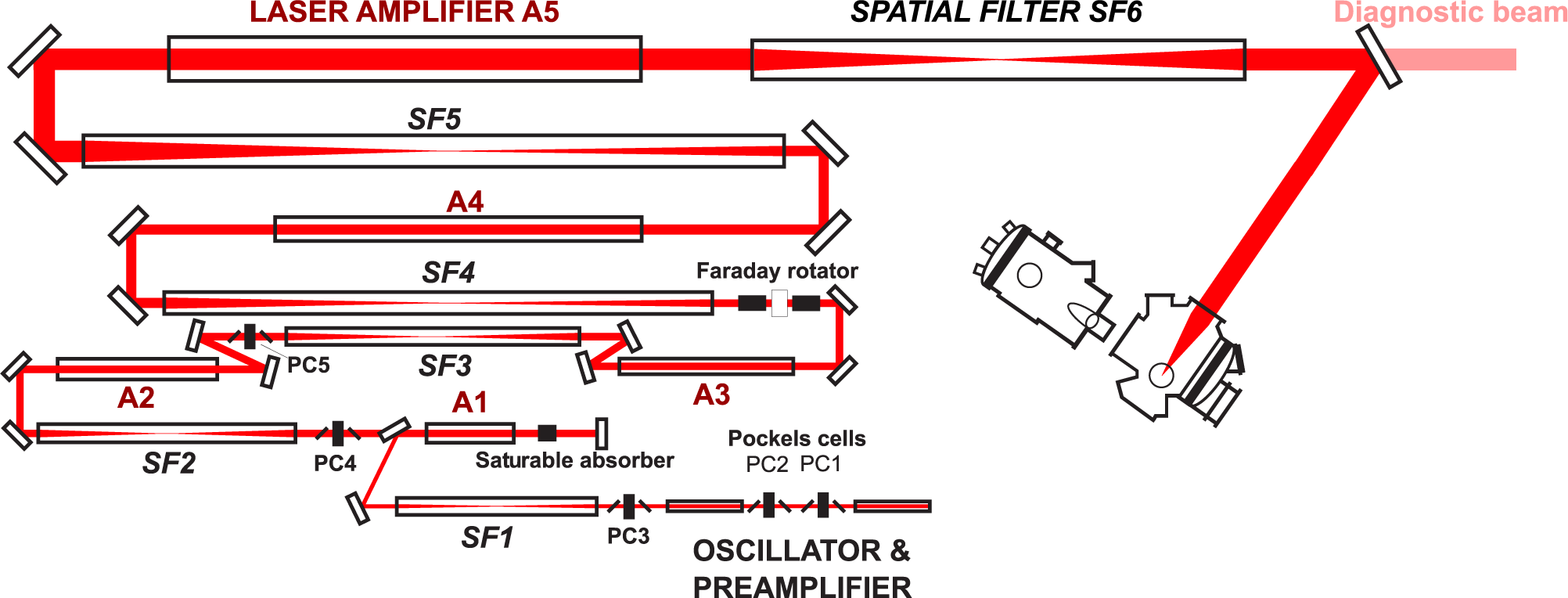
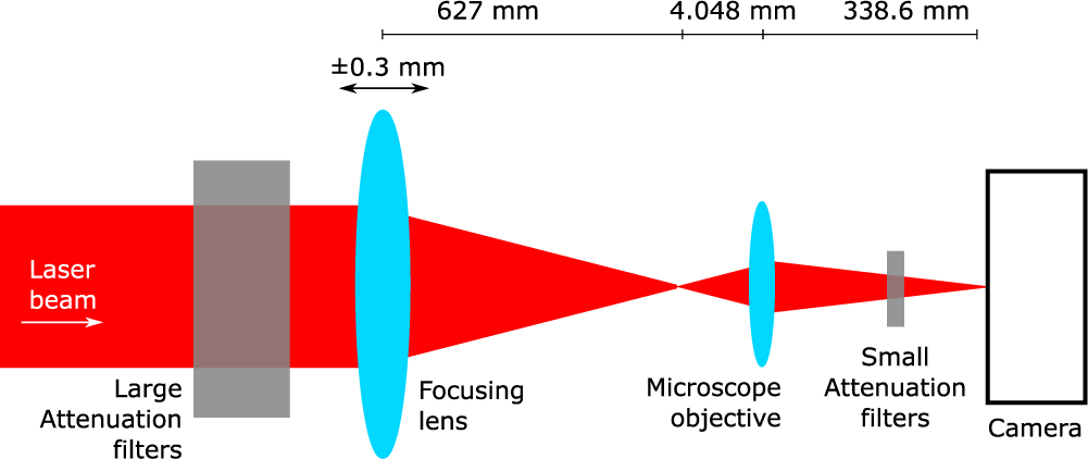


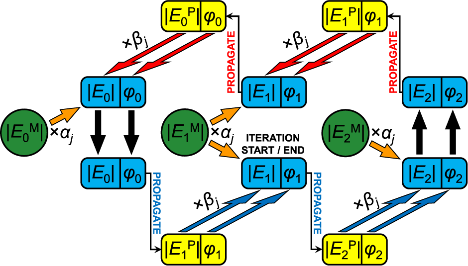


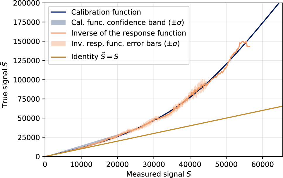


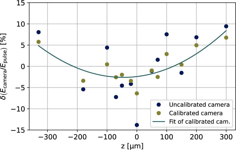


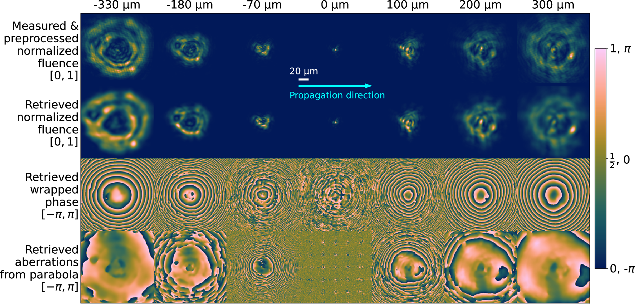


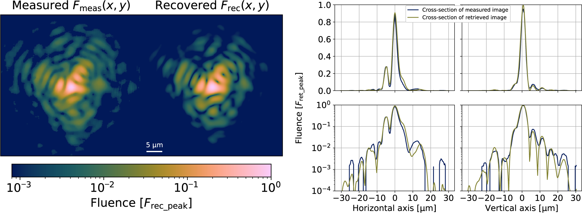

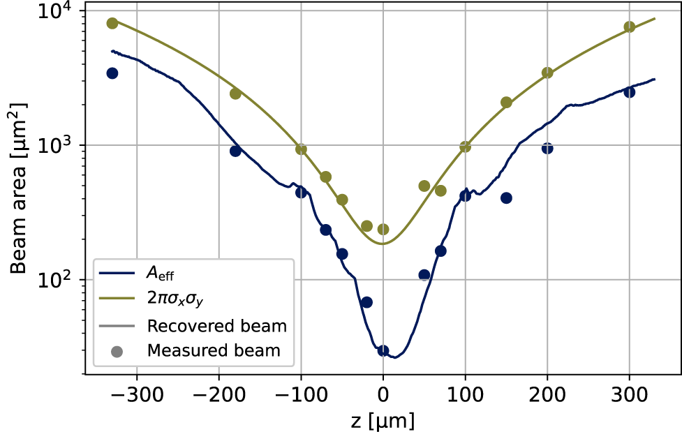


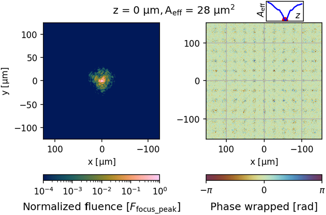


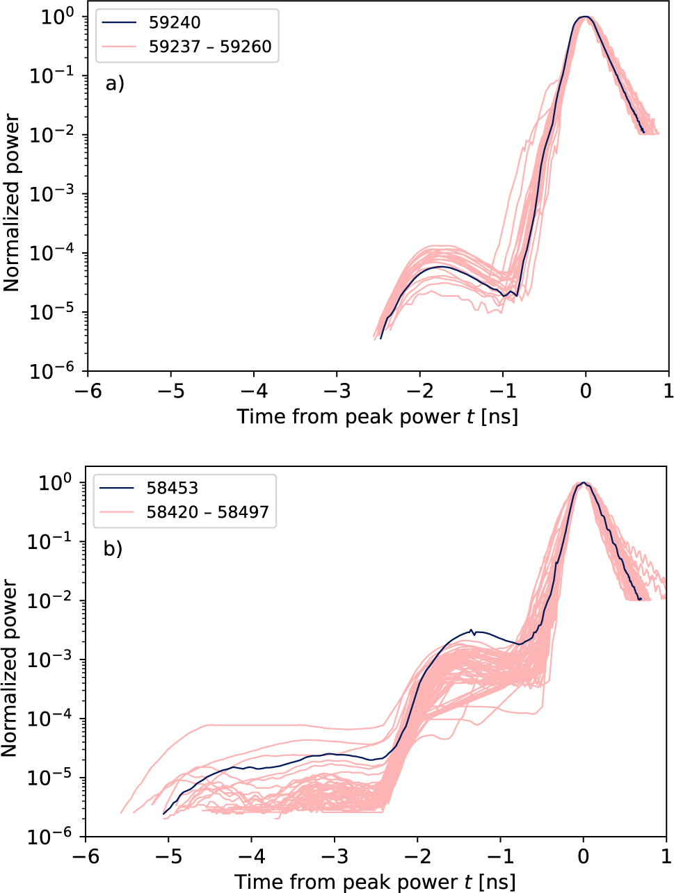

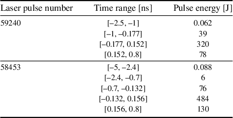
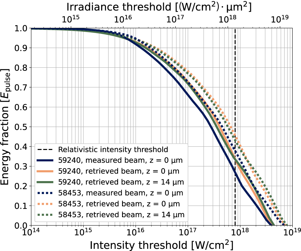


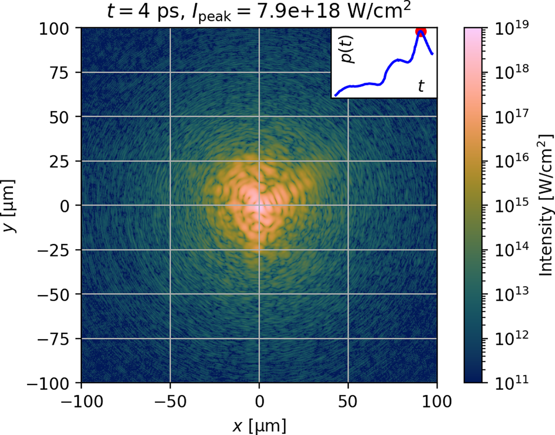

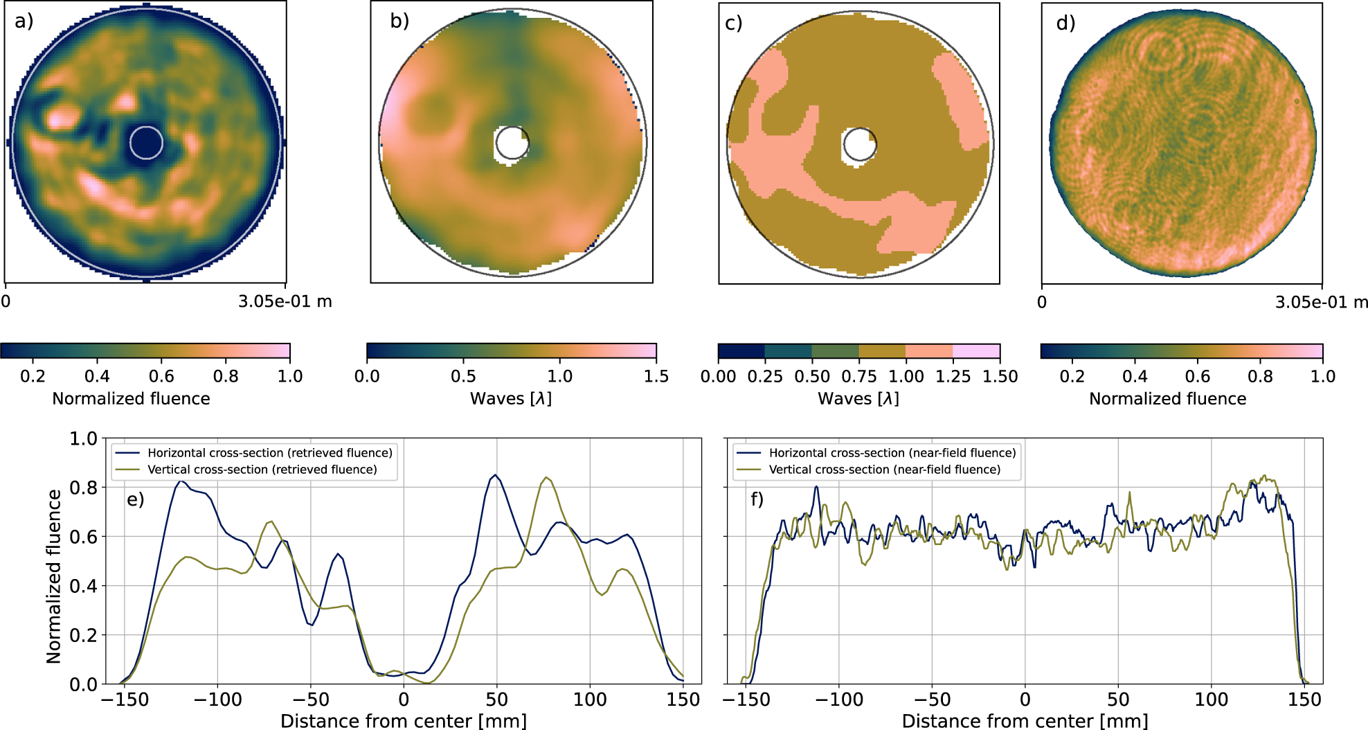


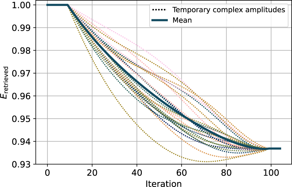


 Open access

