


1. Introduction
In neutrally stratified shallow water, shear-driven turbulence underneath surface waves often features full-depth Langmuir cells (LCs) in the form of pairs of counter-rotating streamwise vortices extending from the water surface to the bottom (Gargett et al. Reference Gargett, Wells, Tejada-Martínez and Grosch2004; Gargett & Wells Reference Gargett and Wells2007; Tejada-Martínez & Grosch Reference Tejada-Martínez and Grosch2007). Field observations and laboratory experiments have shown that the concentration of resuspended sediment in shallow-water Langmuir turbulence exhibits an organized spanwise variation (Gargett et al. Reference Gargett, Wells, Tejada-Martínez and Grosch2004; Dethleff & Kempema Reference Dethleff and Kempema2007). Because sediment resuspension and transport are correlated with the shear stresses at the water bottom (Grant & Madsen Reference Grant and Madsen1986; Grant & Marusic Reference Grant and Marusic2011), it is crucial to make accurate predictions of wall shear stress fluctuations in shallow-water Langmuir turbulence. Recent studies of canonical wall-bounded turbulent flows also show that investigation of the wall shear stress fluctuations can improve the wall-layer model in large-eddy simulation (LES) (Howland & Yang Reference Howland and Yang2018) and help predict turbulence statistics in reduced-order models (Sasaki et al. Reference Sasaki, Vinuesa, Cavalieri, Schlatter and Henningson2019). As a first step to expand these valuable model applications from canonical wall-bounded turbulent flows to flows in coastal environments, we investigate wall shear stress fluctuations in shallow-water Langmuir turbulence in this study.
Streamwise wall shear stress fluctuations in canonical wall turbulence without full-depth LCs have been extensively studied in the literature (Alfredsson et al. Reference Alfredsson, Johansson, Haritonidis and Eckelmann1988; Kravchenko, Choi & Moin Reference Kravchenko, Choi and Moin1993; Jeon et al. Reference Jeon, Choi, Yoo and Moin1999; Miyagi et al. Reference Miyagi, Kimura, Shoji, Saima, Ho, Tung and Tai2000; Colella & Keith Reference Colella and Keith2003; Abe, Kawamura & Choi Reference Abe, Kawamura and Choi2004; Hu, Morfey & Sandham Reference Hu, Morfey and Sandham2006; Örlü & Schlatter Reference Örlü and Schlatter2011; Klewicki Reference Klewicki2012; Keirsbulck, Labraga & GadelHak Reference Keirsbulck, Labraga and GadelHak2012; Diaz-Daniel, Laizet & Vassilicos Reference Diaz-Daniel, Laizet and Vassilicos2017; Gubian et al. Reference Gubian, Stoker, Medvescek, Mydlarski and Baliga2019; Liu, Klaas & Schröder Reference Liu, Klaas and Schröder2019; Wang, Pan & Wang Reference Wang, Pan and Wang2020). At low Reynolds numbers, the streamwise wall shear stress fluctuations are highly correlated with the near-wall coherent structures (Alfredsson et al. Reference Alfredsson, Johansson, Haritonidis and Eckelmann1988; Kravchenko et al. Reference Kravchenko, Choi and Moin1993; Jeon et al. Reference Jeon, Choi, Yoo and Moin1999). As the Reynolds number increases, the large-scale motions (LSMs) originating from the outer layer also impact the near-wall flow through the linear superimposition effect (Brown & Thomas Reference Brown and Thomas1977; Metzger & Klewicki Reference Metzger and Klewicki2001; Abe et al. Reference Abe, Kawamura and Choi2004; Marusic, Mathis & Hutchins Reference Marusic, Mathis and Hutchins2010) and the nonlinear modulation effect (Hutchins & Marusic Reference Hutchins and Marusic2007; Mathis, Hutchins & Marusic Reference Mathis, Hutchins and Marusic2009; Deng, Huang & Xu Reference Deng, Huang and Xu2016; Hwang & Sung Reference Hwang and Sung2017). The former means that the large-scale horizontal velocity fluctuations near the wall are caused by LSMs extending from the outer layer to the near-wall region, and the latter means that the small-scale velocity fluctuations generated locally near the wall are amplified or attenuated by LSMs depending on the sign of the large-scale velocity. Consequently, the statistics of the streamwise wall shear stress fluctuations vary with the Reynolds number. For example, the root-mean-square (r.m.s.) value of the streamwise wall shear stress fluctuations exhibits a logarithmic increase with the Reynolds number (Örlü & Schlatter Reference Örlü and Schlatter2011) for the friction Reynolds number  $Re_\tau \sim {O}(10^2\sim 10^3)$ in numerical simulations (Abe et al. Reference Abe, Kawamura and Choi2004; Hu et al. Reference Hu, Morfey and Sandham2006; Diaz-Daniel et al. Reference Diaz-Daniel, Laizet and Vassilicos2017) and $Re_\tau \sim {O}(10^2\sim 10^7)$ in experiments (Mathis et al. Reference Mathis, Marusic, Chernyshenko and Hutchins2013; Gubian et al. Reference Gubian, Stoker, Medvescek, Mydlarski and Baliga2019; Wang et al. Reference Wang, Pan and Wang2020). The skewness, kurtosis and the probability density of extreme events all grow weakly with the Reynolds number (Keirsbulck et al. Reference Keirsbulck, Labraga and GadelHak2012; Diaz-Daniel et al. Reference Diaz-Daniel, Laizet and Vassilicos2017; Liu et al. Reference Liu, Klaas and Schröder2019). Mathis et al. (Reference Mathis, Marusic, Chernyshenko and Hutchins2013) proposed a predictive model for the streamwise wall shear stress fluctuations by accounting for the linear superimposition and nonlinear modulation effects of LSMs. Their model successfully reproduced the shear stress fluctuations using the outer-layer large-scale streamwise velocity, which was later used to improve the wall-layer model for wall turbulence simulations (Howland & Yang Reference Howland and Yang2018; Yin, Huang & Xu Reference Yin, Huang and Xu2018).
In the presence of full-depth LCs (or Langmuir-type cells), LSMs still exist but are attenuated (Deng et al. Reference Deng, Yang, Xuan and Shen2019; Peruzzi et al. Reference Peruzzi, Vettori, Poggi, Blondeaux, Ridolfi and Manes2021), characterized by the reduction in the contribution of LSMs to the Reynolds stresses in the outer layer. Conversely, full-depth LCs generated by the interaction between wind-driven turbulent currents and water waves fill the whole water column and significantly impact the flow field near the bottom (Gargett & Wells Reference Gargett and Wells2007; Tejada-Martínez & Grosch Reference Tejada-Martínez and Grosch2007; Kukulka, Plueddemann & Sullivan Reference Kukulka, Plueddemann and Sullivan2012; Martinat, Grosch & Gatski Reference Martinat, Grosch and Gatski2014; Sinha et al. Reference Sinha, Tejada-Martínez, Akan and Grosch2015; Deng et al. Reference Deng, Yang, Xuan and Shen2019, Reference Deng, Yang, Xuan and Shen2020). Specifically, the streamwise and spanwise components of the Reynolds normal stresses near the bottom are enhanced by full-depth LCs through the linear superimposition effect (Gargett & Wells Reference Gargett and Wells2007; Tejada-Martínez & Grosch Reference Tejada-Martínez and Grosch2007; Sinha et al. Reference Sinha, Tejada-Martínez, Akan and Grosch2015; Deng et al. Reference Deng, Yang, Xuan and Shen2019). Full-depth LCs also have strong nonlinear interactions with small-scale background turbulent motions (Kukulka et al. Reference Kukulka, Plueddemann and Sullivan2012; Martinat et al. Reference Martinat, Grosch and Gatski2014; Deng et al. Reference Deng, Yang, Xuan and Shen2020), resulting in an organized spanwise variation in turbulence intensity near the bottom (Martinat et al. Reference Martinat, Grosch and Gatski2014; Deng et al. Reference Deng, Yang, Xuan and Shen2020).
Based on the above review on the previous studies of LSMs and full-depth LCs, it is expected that research on the impacts of full-depth LCs on bottom wall shear stress fluctuations in shallow-water Langmuir turbulence would be useful for improving the wall-layer model and sediment resuspension model in coastal flows. Recently, Shrestha & Anderson (Reference Shrestha and Anderson2020) studied the bottom wall shear stresses in shallow-water Langmuir turbulence using wall-modelled LES based on the Craik–Leibovich (CL) equations (Craik & Leibovich Reference Craik and Leibovich1976; Craik Reference Craik1977). The significant impacts of full-depth LCs on wall shear stress fluctuations are evident from the comparison of the instantaneous fields between shallow-water Langmuir turbulence (Shrestha & Anderson Reference Shrestha and Anderson2020) and canonical wall turbulence (Abe et al. Reference Abe, Kawamura and Choi2004; Mathis et al. Reference Mathis, Marusic, Chernyshenko and Hutchins2013). Specifically, Shrestha & Anderson (Reference Shrestha and Anderson2020) found that almost all of the streamwise wall shear stress fluctuations have the same signs as the streamwise velocity induced by full-depth LCs, while the correlation in canonical wall turbulence is lower, approximately 0.3 (Mathis et al. Reference Mathis, Marusic, Chernyshenko and Hutchins2013). Motivated by the pioneering work of Shrestha & Anderson (Reference Shrestha and Anderson2020), systematic studies of the impacts of full-depth LCs on wall shear stress fluctuations in shallow-water Langmuir turbulence are called for.
In the present work we aim to address the following three questions on the impacts of full-depth LCs on the streamwise and spanwise components of bottom wall shear stress fluctuations in neutrally stratified shallow-water Langmuir turbulence.
(i) How do full-depth LCs impact the spatial distribution of bottom wall shear stress fluctuations?
(ii) What are the impacts of full-depth LCs on the statistics of the wall shear stress fluctuations?
(iii) How can the impacts of full-depth LCs on the wall shear stress fluctuations be quantitatively scaled under different flow conditions, and how can their predictive models be developed in shallow-water Langmuir turbulence?
These questions are answered by analysing the wall-resolved LES database of neutrally stratified shallow-water Langmuir turbulence obtained by Deng et al. (Reference Deng, Yang, Xuan and Shen2019). The full-depth LCs are extracted using a triple decomposition technique. The impacts of full-depth LCs are revealed by comparing the results with those in pure shear-driven turbulence without full-depth LCs. Through the investigation of the statistics at different Reynolds numbers, wavenumbers of water waves and turbulent Langmuir numbers (McWilliams, Sullivan & Moeng Reference McWilliams, Sullivan and Moeng1997), the impacts of full-depth LCs on the wall shear stress fluctuations are quantitatively scaled using the velocities induced by full-depth LCs. Based on these scalings, a predictive model is developed. The proposed model establishes a physical foundation for the improvement of wall-layer modelling for coastal flows in the future.
The remainder of this paper is organized as follows. The database of the neutrally stratified shallow-water Langmuir turbulence obtained by wall-resolved LES is introduced in § 2. Section 3 investigates the mechanisms of full-depth LCs governing the spatial distribution of the wall shear stress fluctuations. The impacts of full-depth LCs on the statistics of wall shear stress fluctuations are quantified in § 4. In § 5 a predictive model is proposed and assessed. Sections 3, 4 and 5 address questions (i), (ii) and (iii), respectively. Conclusions are given in § 6.
2. Database and LCs
2.1. Description of database
The wall-resolved LES database of neutrally stratified shallow-water Langmuir turbulence is obtained by solving the following continuity and CL equations:
 $$\begin{gather} \frac{\partial{u}_i}{\partial x_i}=0, \end{gather}$$
 $$\begin{gather}\frac{\partial{{u}_i}}{\partial t} + {{u}_j} \frac{\partial{{u}_i}}{\partial x_j} ={-}\frac{1}{\rho}\frac{\partial {\varPi}}{\partial x_i} + \nu \frac{\partial^2{{u}_i}}{\partial {x_j}\partial {x_j}}+ \frac{\partial{\tau}^{sgs}_{ij}}{\partial x_j}+ \epsilon_{ijk}u^s_j {\omega}_k + {F_i}. \end{gather}$$
As shown in figure 1, the filtered velocities in the streamwise ( $x$ or $x_1$), vertical ( $y$ or $x_2$) and spanwise ( $z$ or $x_3$) directions are $u$ (or $u_1$), $v$ (or $u_2$) and $w$ (or $u_3$), respectively. In the first and second terms on the right-hand side of (2.2), $\varPi$ is the modified pressure in the LES, $\rho$ is the water density and $\nu$ is the kinematic viscosity of water. According to the derivation of the CL equations (Craik & Leibovich Reference Craik and Leibovich1976; Craik Reference Craik1977), $u_i$ corresponds to the velocity induced by mean current and turbulence motions, of which the characteristic frequencies are much lower than the water wave frequencies. Because the high-frequency wave-induced motions are clipped in the CL equations, LES is conducted and a subgrid-scale (SGS) stress tensor term $\tau _{ij}^{sgs}$ is included in the third term on the right-hand side of (2.2) (McWilliams et al. Reference McWilliams, Sullivan and Moeng1997; Tejada-Martínez & Grosch Reference Tejada-Martínez and Grosch2007). The effects of waves on the mean current and turbulence motions are represented by a CL vortex forcing, the last term on the right-hand side of (2.2), where $\epsilon _{ijk}$ is the third-order Levi–Civita symbol, $\omega _i$ is the vorticity and $u_i^s$ is the Stokes drift of water waves. In shallow water, $u_i^s$ is quantified as (Tejada-Martínez & Grosch Reference Tejada-Martínez and Grosch2007)
 \begin{equation} {u}^s_1=u^{s*}\frac{\cosh(2ky)}{2\sinh^2(2kh)},\quad {u}^s_2={u}^s_3=0, \quad y/h\in[0,2], \end{equation}
where  $u^{s*}$ is the wave Stokes drift velocity at the water surface, $k$ is the wavenumber and $h$ is the half-water depth. The term $F_i$ is the imposed pressure gradient corresponding to the tide. The present study focuses on the neutral stratification condition, i.e. no stratification in the flow, and, thus, the effect of the buoyancy force is ignored. The boundary conditions at the water surface $y/h=2$ include no penetration, a constant streamwise wind shear stress $\tau _w$ and a zero spanwise wind shear stress. The no-slip boundary condition is employed at the water bottom $y/h=0$. The periodic boundary condition is applied in the streamwise and spanwise directions.
Sketch of the computational model for shallow-water Langmuir turbulence.

Equations (2.1)–(2.2) are solved using the fractional-step method (Kim & Moin Reference Kim and Moin1985). The spatial discretization utilizes a hybrid spectral/finite-differential scheme on a staggered grid (Deng et al. Reference Deng, Yang, Xuan and Shen2019). The dynamic Smagorinsky model is used to calculate the SGS stress tensor  ${\tau }^{sgs}_{ij}$ (Smagorinsky Reference Smagorinsky1963; Germano et al. Reference Germano, Piomelli, Moin and Cabot1991; Lilly Reference Lilly1992). Details of our simulation schemes and validations can be found in Deng et al. (Reference Deng, Yang, Xuan and Shen2019, Reference Deng, Yang, Xuan and Shen2020).
Using the friction velocity at the water surface  $u_w=\sqrt {\tau _w/\rho }$ and the half-water depth $h$ as the characteristic velocity and length scales, respectively, there are four non-dimensional parameters in the CL equation, including the friction Reynolds number $Re_\tau =u_w h/ \nu$, the turbulent Langmuir number $La_t=\sqrt {(u_w/u^*)(u^*/u^{s*})}$ (Martinat et al. Reference Martinat, Xu, Grosch and Tejada-Martínez2011; Gargett & Grosch Reference Gargett and Grosch2014; Shrestha et al. Reference Shrestha, Anderson, Tejada-Martinez and Kuehl2019; Shrestha & Anderson Reference Shrestha and Anderson2020), the wavenumber of the surface waves $kh$, and the relative strength between the wind stress and the pressure gradient forcing $\psi =u_w/u_{\tau,S}$ (Shrestha et al. Reference Shrestha, Anderson, Tejada-Martinez and Kuehl2019). Here, $u^*=\sqrt {\tau _b/\rho }$ is the total friction velocity corresponding to the total mean bottom shear stress $\tau _b$, and $u_{\tau,S}=\sqrt {\tau _S/\rho }$ is the friction velocity corresponding to the mean bottom shear stress $\tau _S$ induced by the pressure gradient. According to the observation records of full-depth LCs in field experiments, full-depth LCs are present when the tide is relatively weak (Gargett et al. Reference Gargett, Wells, Tejada-Martínez and Grosch2004; Gargett & Wells Reference Gargett and Wells2007; Gargett & Grosch Reference Gargett and Grosch2014). Therefore, following the works of Tejada-Martínez & Grosch (Reference Tejada-Martínez and Grosch2007), Tejada-Martínez et al. (Reference Tejada-Martínez, Grosch, Sinha, Akan and Martinat2012), Sinha et al. (Reference Sinha, Tejada-Martínez, Akan and Grosch2015) and Shrestha & Anderson (Reference Shrestha and Anderson2020), we focus on the cases of $\psi =\infty$, i.e. $u^*/u^{s*}=1$, to exclusively study the effect of full-depth LCs in the present study. The impacts of the pressure gradients are briefly discussed in § 5.4.
The values of the other three parameters are listed in table 1. Among the nine cases, pure shear-driven turbulence with  $La_t=\infty$ (case 7) is compared with the shallow-water Langmuir turbulence cases to illustrate the impacts of full-depth LCs on the wall shear stresses. As reported by Tejada-Martínez & Grosch (Reference Tejada-Martínez and Grosch2007), Sinha et al. (Reference Sinha, Tejada-Martínez, Akan and Grosch2015) and Shrestha, Anderson & Kuehl (Reference Shrestha, Anderson and Kuehl2018), for shallow-water to intermediate water waves ( $kh<{\rm \pi} /2$) with $0.38< La_t<1$, the spanwise length scales of full-depth LCs and the spatial distribution patterns of the velocities induced by full-depth LCs are not significantly influenced by $La_t$ and $kh$. At low $La_t$ ( $La_t<0.38$) the full-depth LCs are weaker and narrower than $La_t>0.38$ (Shrestha et al. Reference Shrestha, Anderson and Kuehl2018). Under the condition of deep water waves $kh=5.0$, the full-depth LCs are deformed with significantly weakened upwelling motions (Shrestha et al. Reference Shrestha, Anderson and Kuehl2018). To conduct a systematic analysis on the effects of full-depth LCs, different flow conditions in the ranges of $0.38< La_t<1$ and $kh<{\rm \pi} /2$ are firstly considered in cases 1–6 with $Re_\tau$ varying from $1000$ to $395$ (cases 1–3), $kh$ ranging from $0.5$ to $5.0$ (cases 1, 4, 5, 8), and $La_t$ changing from $0.7$ to $0.9$ (cases 1 and 6). The effects of deformed full-depth LCs occurring at low $La_t$ or high $kh$ are explored using case 8 ( $La_t=0.3$) and case 9 ( $kh=5$), respectively.
Computational parameters in various cases. The grid numbers in the streamwise, vertical and spanwise directions are  $N_x$, $N_y$ and $N_z$, respectively. The grid resolutions in the streamwise and spanwise directions are $\Delta x^+$ and $\Delta z^+$, respectively. The minimal grid resolution in the vertical direction is $\Delta y^+_{min}$. Other variables are defined in the text.

Owing to the limitation of the present computer power, the Reynolds number in the present wall-resolved LES is much lower than the realistic values  $Re_\tau =O(10^6)$. However, $Re_\tau =1000$ is sufficiently high for shallow-water Langmuir turbulence to capture the typical high-Reynolds-number effects as in canonical wall turbulence. To be specific, LSMs in canonical high-Reynolds-number wall turbulence lead to a bimodal shape in the profile of the r.m.s. value of the streamwise velocity fluctuations (Smits, McKeon & Marusic Reference Smits, McKeon and Marusic2011), and similarly, full-depth LCs in shallow-water Langmuir turbulence at $Re_\tau =1000$ also induce a bimodal profile of the r.m.s. value (Deng et al. Reference Deng, Yang, Xuan and Shen2019). Furthermore, both the LSMs in canonical high-Reynolds-number wall turbulence and full-depth LCs at $Re_\tau =1000$ impose a nonlinear modulation effect on small-scale turbulence (Mathis et al. Reference Mathis, Hutchins and Marusic2009; Deng et al. Reference Deng, Yang, Xuan and Shen2020).
The size of the computational domain is  $L_x \times L_y \times L_z = 8{\rm \pi} h \times 2h \times 16{\rm \pi} h/3$, which contains two pairs of full-depth LCs in the $z$-direction for cases 1–6 (Deng et al. Reference Deng, Yang, Xuan and Shen2019), and three pairs of full-depth LCs for case 8 (shown in § 5.4). The number of water waves in the domain is $L_x /\lambda =L_x /(2{\rm \pi} /k)=4kh$, with $\lambda$ being the wavelength of the wave. As reported in our previous studies (Deng et al. Reference Deng, Yang, Xuan and Shen2019, Reference Deng, Yang, Xuan and Shen2020), the meandering of the large-scale streaks of streamwise velocity can be observed in both the present computational domain and a larger domain of $32{\rm \pi} h \times 2h \times 64{\rm \pi} h/3$, and the statistics of the LCs parts and the background turbulence parts of velocities fluctuations obtained in these two domains are consistent. This means that $L_x=8{\rm \pi} h$ is sufficiently large to capture the meandering of LSMs. The grid mesh is evenly distributed in the $x$- and $z$-directions and is stretched in the $y$-direction. The first mesh centres off the surface and the bottom is located within $\Delta y^+=1$. Hereinafter, the superscript ‘ $+$’ denotes values non-dimensionalized by the wall unit $\delta _\upsilon =\nu /u_w$ and friction velocity $u_w$. The grid resolution satisfies the requirement of wall-resolved LES, namely, $50\leqslant \Delta x^+ \leqslant 130$, $15\leqslant \Delta z^+\leqslant 35$ and $\Delta y^+_{min}\leqslant 1$ (Chapman Reference Chapman1979; Choi & Moin Reference Choi and Moin2012). Discussions on the choices of simulation parameters can be found in Deng et al. (Reference Deng, Yang, Xuan and Shen2019). It was confirmed in Deng et al. (Reference Deng, Yang, Xuan and Shen2019) that the turbulence statistics obtained from the wall-resolved LES of shallow-water Langmuir turbulence using the CL equations agree with experimental results (also see Tejada-Martínez & Grosch Reference Tejada-Martínez and Grosch2007). Therefore, the database is used in the present study to investigate the impacts of full-depth LCs on the statistics of the bottom wall shear stress fluctuations.
2.2. Extraction of full-depth LCs
Full-depth LCs are extracted using the following triple decomposition (Tejada-Martínez & Grosch Reference Tejada-Martínez and Grosch2007):
 \begin{equation} {{u}_i}=\langle{{u_i}}\rangle+{u}_i^\prime= \langle{{u_i}}\rangle+u_i^L+u_i^T. \end{equation}
Here  $\langle {{u_i}} \rangle$ is the mean current based on time and plane averaging, and $u_i^\prime$ represents the velocity fluctuations induced by turbulence motions. The velocity fluctuations can be further decomposed into an LCs part $u^L_i$ and a background turbulence part $u_i^T$. The LCs part $u_i^L$ is defined as
 \begin{equation} u_i^L=\frac{1}{L_x}\int^{L_x}_0{u}_i^\prime \,\mathrm{d}\kern0.7pt x. \end{equation}
Because the present computational domain can capture the meandering of LSMs, the streamwise averaging is sufficient to separate full-depth LCs from other meandering structures, and, thus, time averaging is not applied in (2.5). In pure shear-driven turbulence  $u_i^L$ corresponds to the velocity induced by Couette cells (CCs), owing to their similarity to the cells in turbulent Couette flows (Tejada-Martínez & Grosch Reference Tejada-Martínez and Grosch2007). The above triple decomposition has been used to extract the CCs in turbulent Couette flows (Papavassiliou & Hanratty Reference Papavassiliou and Hanratty1997) and full-depth LCs in shallow-water Langmuir turbulence (Tejada-Martínez & Grosch Reference Tejada-Martínez and Grosch2007; Deng et al. Reference Deng, Yang, Xuan and Shen2019). Similar triple decomposition techniques were also used to study the coherent motions induced by streamwise-aligned roughness and riblets (Raupach & Shaw Reference Raupach and Shaw1982; Choi, Moin & Kim Reference Choi, Moin and Kim1993; Jimenez et al. Reference Jimenez, Uhlmann, Pinelli and Kawahara2001; Garcia-Mayoral & Jimenez Reference Garcia-Mayoral and Jimenez2011; Jelly, Jung & Zaki Reference Jelly, Jung and Zaki2014; Seo, Garcia-Mayoral & Mani Reference Seo, Garcia-Mayoral and Mani2015; Scherer et al. Reference Scherer, Uhlmann, Kidanemariam and Krayer2022).
Corresponding to the triple decomposition (2.4), the wall shear stress, defined as
 \begin{equation} {\tau_{i2}}= \mu \left. \frac{\partial u_i}{\partial y} \right |_{y=0}, \end{equation}
can also be decomposed into
 \begin{equation} {\tau_{i2}}= \langle{\tau_{i2}}\rangle + {\tau_{i2}}^\prime= \langle{\tau_{i2}}\rangle + {\tau_{i2}}^L + {\tau_{i2}}^T. \end{equation}
According to the no-slip bottom boundary condition and the continuity equation,  ${\tau _{22}}=0$ strictly holds. Furthermore, when the flow develops into an equilibrium state, the mean wall shear stress is balanced by the wind shear stress at the water surface, and, therefore, $\langle {\tau _{12}}\rangle = \tau _w$ and $\langle {\tau _{32}}\rangle =0$. In the present study we focus on the fluctuations ${\tau _{12}}^\prime$ and ${\tau _{32}}^\prime$ and their LCs and background turbulence parts.
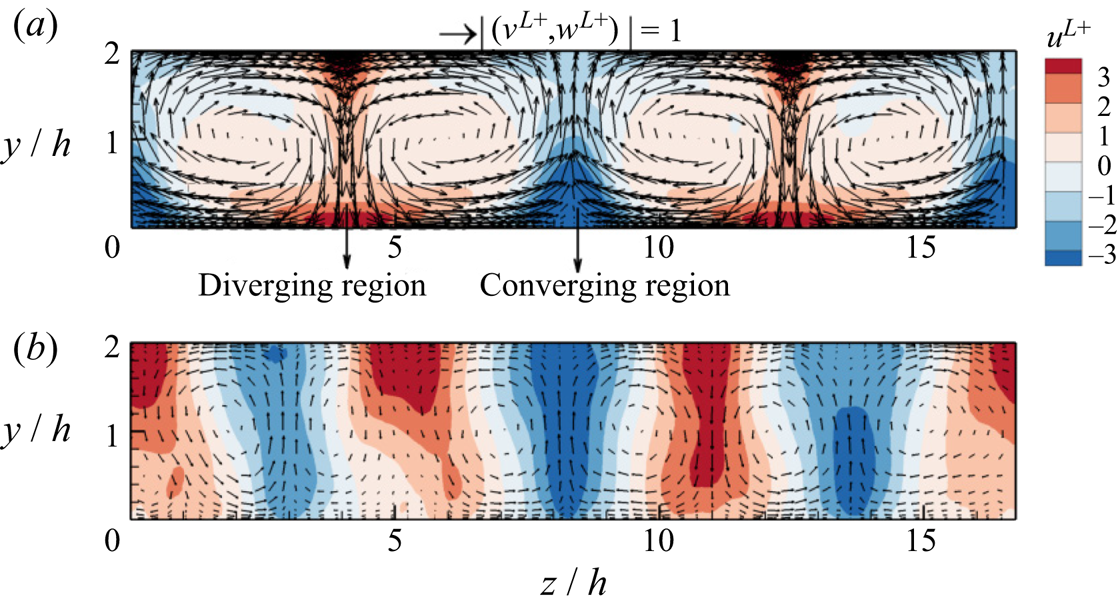
Figure 2 compares the instantaneous flow fields between the full-depth LCs in shallow-water Langmuir turbulence (case 1) and CCs in pure shear-driven turbulence (case 7). Both full-depth LCs and CCs appear as counter-rotating streamwise vortex pairs. However, the streamwise and spanwise velocities induced by full-depth LCs are more intense than those of CCs, especially near the water bottom. Owing to the strong footprint of full-depth LCs near the bottom, the wall shear stress fluctuations in shallow-water Langmuir turbulence are significantly altered by full-depth LCs, as shown in the results in the following sections.
Instantaneous fields of  $u_i^{L}$ in (a) shallow-water Langmuir turbulence (case 1) and (b) pure shear-driven turbulence (case 7). The contours are $u^{L+}$ and the vectors are $(v^{L+},w^{L+})$. The near-bottom diverging and converging flow regions induced by full-depth LCs are marked in (a).
3. Spatial distribution of wall shear stress fluctuations
In this section the effects of full-depth LCs on the spatial variation of the wall shear stress fluctuations are first illustrated by comparing their instantaneous fields with those in pure shear-driven turbulence. Next, how full-depth LCs dominate the spatial patterns of the stresses is elucidated by analysing the joint probability density function (j.p.d.f.) of the LCs part of the velocity and the stresses. Cases 1 and 7 are selected as the representatives of shallow-water Langmuir turbulence and pure shear-driven turbulence, respectively. The other cases listed in table 1 are used to develop and validate the predictive model in § 5.
3.1. Spatial patterns of wall shear stress fluctuations
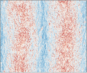
Figure 3 compares the contours of instantaneous wall shear stress fluctuations between shallow-water Langmuir turbulence (case 1) and pure shear-driven turbulence (case 7). The dashed lines in figure 3(a,b) divide the  $x$–
$x$– $z$ plane into regions with positive and negative $u^L$, while the dash-dotted lines in figure 3(c,d) separate the regions with positive $w^L$ from those with negative $w^L$. Here, the values of the LCs parts of the streamwise velocity $u^L$ and spanwise velocity $w^L$ are taken at a reference height of $y/h=0.1$ ( $y^+=100$), where the peak r.m.s. value of $u^L$ in shallow-water Langmuir turbulence occurs (Deng et al. Reference Deng, Yang, Xuan and Shen2019). Figure 3(a) shows that in shallow-water Langmuir turbulence, the positively and negatively valued streamwise wall shear stress fluctuations ${\tau _{12}}^\prime$ are accumulative in the regions with the same signs of $u^L$, forming streamwise-elongated large-scale streaks. In contrast, such organized streamwise-elongated streaks are not observed in pure shear-driven turbulence (figure 3b), where positive-valued (negative-valued) ${\tau _{12}}^\prime$ also occurs in the regions with negative $u^L$ (positive $u^L$). In other words, the correlation between ${\tau _{12}}^\prime$ and $u^L$ is more pronounced in shallow-water Langmuir turbulence than in pure shear-driven turbulence. This comparison illustrates the dominant role played by full-depth LCs in the spatial pattern of streamwise wall shear stress fluctuations.
Instantaneous fields of wall shear stress fluctuations. (a,b) The streamwise wall shear stress fluctuation  $\tau _{12}^\prime$ in shallow-water Langmuir turbulence (case 1) and pure shear-driven turbulence (case 7), respectively. (c,d) The spanwise wall shear stress fluctuation $\tau _{32}^\prime$ in case 1 and case 7, respectively. The LCs parts of the streamwise velocity $u^L$ and spanwise velocity $w^L$ are taken at a reference height of $y/h=0.1$ ( $y^+=100$ at $Re_\tau =1000$).

The instantaneous spanwise wall shear stress fluctuation  ${\tau _{32}}^\prime$ is also influenced by full-depth LCs. In pure shear-driven turbulence ${\tau _{32}}^\prime$ is distributed irregularly in the $x$–
$x$– $z$ plane (figure 3d). In contrast, in shallow-water Langmuir turbulence ${\tau _{32}}^\prime$ exhibits an organized distribution (figure 3c). The events of small-magnitude ${\tau _{32}}^\prime$ gather in the near-bottom converging region with negative $u^L$, while the events of large-magnitude ${\tau _{32}}^\prime$ appear in a bristle form in the diverging region with positive $u^L$ (see figures 3a,c and 2a). In the diverging region, positive- and negative-valued ${\tau _{32}}^\prime$ concentrates on the sides with positive and negative $w^L$, respectively, forming streamwise-elongated streaks. The above observation indicates that the spanwise distribution of the streaks of ${\tau _{32}}^\prime$ is dependent on both the LCs part of the streamwise velocity $u^L$ and the LCs part of the spanwise velocity $w^L$. Shrestha & Anderson (Reference Shrestha and Anderson2020) found similar patterns based on wall-modelled LES. The similarity between the wall-modelled LES results of Shrestha & Anderson (Reference Shrestha and Anderson2020) and the present wall-resolved LES results suggests a strong impact of full-depth LCs on the background turbulence part of the wall shear stress fluctuations. This point is discussed in more detail in the next section.
3.2. Mechanisms of full-depth LCs influencing the spatial patterns of wall shear stress fluctuations
In this section we analyse the j.p.d.f. of the LCs parts of velocities and the wall shear stress fluctuations to conduct a quantitative investigation of the observation in figure 3. Figure 4 shows the contours of  $P(u^{L}, {\tau _{12}}^{\prime })$, the j.p.d.f. of the LCs part of velocity $u^{L}$ at $y/h=0.1$ and the streamwise wall shear stress fluctuation ${\tau _{12}}^{\prime }$. The results in cases 1 and 7 are contrasted to demonstrate the differences between shallow-water Langmuir turbulence and pure shear-driven turbulence. In the following analyses of j.p.d.f., the LCs parts of velocities $u^{L}$ and $w^{L}$ are all evaluated at $y/h=0.1$ ( $y^+=100$ at $Re_\tau =1000$) without specification. It is seen from figure 4 that the contours of $P(u^{L}, \tau _{12}^{\prime })$ exhibit two peaks for both flows. Around the upper peak with positive $u^{L}$, the probability of positive ${\tau _{12}}^{\prime }$ is higher in shallow-water Langmuir turbulence than in pure shear-driven turbulence. Around the lower peak with negative $u^{L}$, positive ${\tau _{12}}^{\prime }$ is rarer in shallow-water Langmuir turbulence. These features of $P(u^{L}, {\tau _{12}}^{\prime })$ in the presence of full-depth LCs are consistent with the organized streaks of ${\tau _{12}}^{\prime }$ observed in figure 3(a).
Contours of the j.p.d.f. of  $u^{L}$ at $y/h=0.1$ ( $y^+=100$) and $\tau _{12}^{\prime }$ at $y/h=0$, $P(u^{L}, \tau _{12}^{\prime })$. (a,b) Contours obtained from shallow-water Langmuir turbulence with full-depth LCs (case 1) and pure shear-driven turbulence with CCs (case 7), respectively.

Because  ${\tau _{12}}^{\prime }$ consists of an LCs part ${\tau _{12}}^{L}$ and a background turbulence part ${\tau _{12}}^{T}$ (2.7), we further study the impacts of full-depth LCs on $P(u^{L}, {\tau _{12}}^{L})$ and $P(u^{L}, {\tau _{12}}^{T})$. Figure 5 depicts $P(u^{L}, {\tau _{12}}^{L})$ and $P(u^{L}, {\tau _{12}}^{T})$ using red isopleths and coloured contours, respectively. As shown, the contours of $P(u^{L}, {\tau _{12}}^{L})$ are nearly straight lines in both shallow-water Langmuir turbulence and pure shear-driven turbulence. In other words, ${\tau _{12}}^{L+}= \alpha _1 u^{L+}$ holds approximately, indicating a linear superimposition effect of $u^{L}$ on ${\tau _{12}}^{\prime }$ through ${\tau _{12}}^{L}$. Here, $\alpha _1$ is the slope of the straight line and its value is further discussed in § 5.1. The stronger intensity of the LC part of velocity $u^{L}$ (figure 2) leads to a larger magnitude of the linearly superimposed ${\tau _{12}}^{L}$ in shallow-water Langmuir turbulence than in pure shear-driven turbulence. As a result, large-magnitude ${\tau _{12}}^{L}$ events occur more frequently in shallow-water Langmuir turbulence (red isopleths in figure 5).
Joint probability density functions  $P(u^{L}, {\tau _{12}}^{T})$ and $P(u^{L}, {\tau _{12}}^{L})$ in (a) shallow-water Langmuir turbulence (case 1) and (b) pure shear-driven turbulence (case 7). The coloured contours are $P(u^{L}, {\tau _{12}}^{T})$ and the red isopleths are $P(u^{L}, {\tau _{12}}^{T})=0.5$ and $1.2$. The horizontal arrows mark the width of the isopleth $P(u^{L}, {\tau _{12}}^{T})=0.02$.

The j.p.d.f.  $P(u^{L}, {\tau _{12}}^{T})$ (coloured contours in figure 5) is also influenced by full-depth LCs through a nonlinear modulation effect on ${\tau _{12}}^{T}$. In both shallow-water Langmuir turbulence and pure shear-driven turbulence, the contours of $P(u^{L}, {\tau _{12}}^{T})$ are asymmetrical about the horizontal line $u^{L}=0$, suggesting a nonlinear effect of $u^{L}$ on ${\tau _{12}}^{T}$. Specifically, the width of the contours of $P(u^{L}, {\tau _{12}}^{T})$ in the ${\tau _{12}}^{T}$-axis direction is larger in the upper half of the $u^{L}$– ${\tau _{12}}^{T}$ plane with positive $u^{L}$ than in the lower half with negative $u^{L}$. This behaviour of the j.p.d.f. indicates the amplification and suppression of ${\tau _{12}}^{T}$ in the regions with positive and negative $u^{L}$, respectively, similar to the modulation effect of LSMs on near-wall turbulence found in canonical wall turbulence (Marusic et al. Reference Marusic, Mathis and Hutchins2010). Comparing figures 5(a) with 5(b), the width of the isopleth $P(u^{L}, {\tau _{12}}^{T})=0.02$ (indicated by the horizontal arrows) near the upper peak with positive $u^{L}$ is shown to be comparable in the two flows, while near the lower peak with negative $u^{L}$, it is smaller in shallow-water Langmuir turbulence than in pure shear-driven turbulence. This observation indicates that full-depth LCs impose a stronger suppression effect on ${\tau _{12}}^{T}$ in the region with negative $u^{L}$ than CCs.
The relationship among  $P(u^{L}, {\tau _{12}}^{\prime })$, $P(u^{L}, {\tau _{12}}^{T})$ and $P(u^{L}, {\tau _{12}}^{L})$ can be further quantified using the following analyses. Based on the linear relationship ${\tau _{12}}^{L+}=\alpha _1 u^{L+}$ pointed out above, $P(u^{L}, {\tau _{12}}^{\prime })$ can be transformed into $P(u^{L}, {\tau _{12}}^{T})$ as
 \begin{equation} P (u^{L+}, {\tau_{12}}^{\prime+}) = \left|\boldsymbol{\mathsf{J}}\right|^{{-}1} P(u^{L+}, {\tau_{12}}^{T+}={\tau_{12}}^{\prime+}-\alpha_1u^{L+}), \end{equation}
where  $J$ is the Jacobian of the coordinate transformation from $(u^{L+}, {\tau _{12}}^{T+})$ to $(u^{L+}, {\tau _{12}}^{\prime +})$ and ‘ $|~ |$’ represents the determinant of a matrix. Using the relationship ${\tau _{12}}^{\prime +} = \alpha _1 u^{L+} + {\tau _{12}}^{T+}$, $\boldsymbol{\mathsf{J}}$ can be expressed as
 \begin{equation} \boldsymbol{\mathsf{J}}=\frac{\partial
(u^{L+}, {\tau_{12}}^{\prime+})}{\partial (u^{L+},
{\tau_{12}}^{T+})}=\begin{pmatrix} 1 & 0 \\
\alpha_1 & 1 \\ \end{pmatrix}.
\end{equation}
\begin{equation} \boldsymbol{\mathsf{J}}=\frac{\partial
(u^{L+}, {\tau_{12}}^{\prime+})}{\partial (u^{L+},
{\tau_{12}}^{T+})}=\begin{pmatrix} 1 & 0 \\
\alpha_1 & 1 \\ \end{pmatrix}.
\end{equation}
As a result, (3.1) can be further simplified into
 \begin{equation} P (u^{L+}, {\tau_{12}}^{\prime+}) = P(u^{L+}, {\tau_{12}}^{T+}={\tau_{12}}^{\prime+}-\alpha_1u^{L+}). \end{equation}
According to (3.3),  $P(u^{L}, {\tau _{12}}^{\prime })$ can be obtained by shifting $P(u^{L}, {\tau _{12}}^{T})$ in the ${\tau _{12}}^{T}$-axis by a distance of $\alpha _1u^{L+}$ (or ${\tau _{12}}^{L+}$). In (3.3) the j.p.d.f.s $P(u^{L}, {\tau _{12}}^{L})$ and $P(u^{L}, {\tau _{12}}^{T})$ manifest the linear superimposition effect and nonlinear modulation effect, respectively. It is shown below (figure 14 in § 5.1) that $\tau _{12}^{L}$ is induced by a ‘top–down’ mechanism of $u^L$, which is similar to that of LSMs found in wall turbulence (Scherer et al. Reference Scherer, Uhlmann, Kidanemariam and Krayer2022). According to the definition of wall shear stress (2.6), $\tau _{12}^T$ is determined by near-bottom $u^T$, which is amplified/suppressed by the positive/negative energy production correlated to the local positive/negative vertical gradient of $u^L$ (Deng et al. Reference Deng, Yang, Xuan and Shen2020). Therefore, the strong linear superimposition effect and nonlinear modulation effect of full-depth LCs lead to the features of $P(u^{L}, {\tau _{12}}^{\prime })$, which correspond to organized streamwise-elongated streaks of ${\tau _{12}}^{\prime }$ (figure 3a).
Particularly on the lower half-plane with negative  $u^L$, the width of $P(u^{L}, \tau _{12}^{T})$ on the positive side of $\tau _{12}^{T}$ shrinks owing to the suppression effect of negative $u^L$ (figure 5a), and after shifting towards the negative direction of the $\tau _{12}^\prime$-axis (or $\tau _{12}^T$-axis) by a distance of $|\tau _{12}^{L}|$, the contours of the resultant $P(u^{L}, \tau _{12}^{\prime })$ in (3.3) are mostly located on the side of negative $\tau _{12}^\prime$ (figure 4a). On the upper half-plane with positive $u^L$, the width of $P(u^{L}, {\tau _{12}}^{T})$ in the $\tau _{12}^{T}$-axis expands on the positive side of $\tau _{12}^T$ (figure 5a). After a shift towards positive $\tau _{12}^T$ ( $\tau _{12}^\prime$) by a distance of $\tau _{12}^L$, a large portion of the resultant $P(u^{L}, {\tau _{12}}^{\prime })$ is located on the side of positive $\tau _{12}^\prime$ (figure 4a). Therefore, the correlation between $\tau _{12}^\prime$ and $u^L$ is strong in shallow-water Langmuir turbulence (figures 3a, 4a). It should be noted that for positive $u^L$, there is still a portion of the contours of $P(u^{L}, {\tau _{12}}^{\prime })$ on the negative side of $\tau _{12}^{\prime }$ (figure 4a), since $P(u^{L}, {\tau _{12}}^{T})$ also expands on the side of negative $\tau _{12}^{T}$ and the value of positive $\tau _{12}^L$ is not large enough (figure 5a). Comparing $P(u^{L}, \tau _{12}^{\prime })$ in the lower half-plane with that in the upper half-plane, it can be observed that the correlation between negative $\tau _{12}^\prime$ and negative $u^L$ is more pronounced than that of the positive values (figure 4a).
The above discussions are on the streamwise wall shear stress fluctuations  ${\tau _{12}}^{\prime }$. Next, we investigate the spanwise component ${\tau _{32}}^{\prime }$. To conduct quantitative analyses of the impact of full-depth LCs on the spatial pattern of ${\tau _{32}}^{\prime }$ shown in figure 3(c), figure 6 depicts the j.p.d.f. ${P(w^{L}, \tau _{32}^{\prime })}$ under the conditions of $u^{L}>0$ and $u^{L}<0$. In pure shear-driven turbulence the contours of ${P(w^{L}, \tau _{32}^{\prime })}$ under the conditions of $u^{L}>0$ and $u^{L}<0$ are similar to each other. Particularly the contours shown in figure 6(c,d) are both approximately symmetric about the horizontal line $w^{L}=0$. These observations indicate that ${\tau _{32}^{\prime }}$ is almost independent of $u^{L}$ and $w^{L}$, and, thus, ${\tau _{32}}^\prime$ appears irregular in figure 3(d). In contrast, in shallow-water Langmuir turbulence ${P(w^{L}, \tau _{32}^{\prime })}$ shows a strong dependence of ${\tau _{32}^{\prime }}$ on both $u^{L}$ and $w^{L}$. The contours of ${P(w^{L}, \tau _{32}^{\prime })}$ under the condition of $u^{L}>0$ (figure 6a) exhibit two peaks in the first and third quadrants where the signs of $w^{L}$ and ${\tau _{32}^{\prime }}$ are the same, while those under the condition of $u^{L}<0$ (figure 6b) show only one peak at the origin. The above features correspond to the organized streaks of ${\tau _{32}^{\prime }}$ located in the regions with positive $u^{L}$ (figure 3c).
Contours of the j.p.d.f.  ${P(w^{L}, \tau _{32}^{\prime })}$. (a,b) Contours of ${P(w^{L}, \tau _{32}^{\prime })}$ under the conditions of $u^{L}>0$ and $u^{L}<0$, respectively, in shallow-water Langmuir turbulence (case 1). (c,d) Contours of ${P(w^{L}, \tau _{32}^{\prime })}$ for positive and negative $u^{L}$, respectively, in shear-driven turbulence (case 7).

To further investigate the effects of  $u^L$ and $w^L$ on the spanwise wall shear stress fluctuation ${\tau _{32}}^{\prime }$, figure 7 shows ${P(w^{L}, \tau _{32}^{L})}$ and ${P(w^{L}, \tau _{32}^{T})}$ under the conditions of $u^{L}>0$ and $u^{L}<0$. As shown by the red isopleths, $\tau _{{32}}^{L+}$ is approximately a linear function of $w^{L+}$, i.e. ${\tau _{32}}^{L+}=\alpha _3w^{L+}$. This linear function indicates a linear superimposition effect of $w^{L}$ on ${\tau _{32}}^{\prime }$, which is confirmed later in § 5.1 (figure 14) to be induced by a top–down mechanism of $w^L$. In comparison with pure shear-driven turbulence, the magnitude of $w^{L}$ near the bottom is larger in shallow-water Langmuir turbulence (figure 2), which consequently causes a larger magnitude of ${\tau _{32}}^{L}$. Furthermore, it is evident from figure 2(a) that a large magnitude of $w^{L}$ mainly occurs in the near-bottom diverging region with positive $u^{L}$. As a result, the contour peaks in figure 7(a) for $u^{L}>0$ occur at larger magnitudes of $w^{L}$ than in figure 7(b) for $u^{L}<0$.
Joint probability density functions  ${P(w^{L}, \tau _{32}^{T})}$ (the coloured contours) and ${P(w^{L}, \tau _{32}^{L})}$ (the red isopleths) in (a,b) shallow-water Langmuir turbulence (case 1) and (c,d) pure shear-driven turbulence (case 7); (a,c) are under the condition of $u^{L}>0$, and (b,d) are under the condition of $u^{L}<0$. The horizontal arrows in (a,b) mark the width of the isopleth ${P(w^{L}, \tau _{32}^{T})}=0.02$.

In figure 7(a,b) the contours of  $P(w^{L}, {\tau _{32}}^{T})$ are approximately symmetric about the horizontal line $w^{L} = 0$, and, thus, the impact of the signs of $w^{L}$ on ${\tau _{32}}^{T}$ is weak. Conversely, the contour pattern of $P(w^{L}, {\tau _{32}}^{T})$ in figure 7(a) is different from that in figure 7(b), indicating a nonlinear effect of $u^{L}$ on ${\tau _{32}}^{T}$. The width of the contours of $P(w^{L}, {\tau _{32}}^{T})$ in the ${\tau _{32}}^{T}$-axis direction is larger under the condition of $u^{L}>0$ than that under the condition of $u^{L}<0$, demonstrating the amplification and attenuation of ${\tau _{32}}^{T}$ by positive and negative $u^{L}$, respectively. Therefore, it is the LCs part of the streamwise velocity $u^{L}$ but not the spanwise velocity $w^{L}$ that imposes a nonlinear modulation effect on ${\tau _{32}}^{T+}$ in shallow-water Langmuir turbulence. Since $\tau _{32}^T$ is contributed by the background turbulence fluctuations $w^T$ near the bottom, the modulation effect of $u^L$ on $\tau _{32}^T$ is consistent with that on $w^T$ through the local energy production related to the local shear of the vertical gradient of $u^L$. In pure shear-driven turbulence the nonlinear modulation effect of $u^{L}$ on ${\tau _{32}}^T$ is weak, because the difference in the contours of ${P(w^{L}, \tau _{32}^{T})}$ under the conditions of $u^{L}>0$ and $u^{L}<0$ (figure 7c,d) is insignificant.
Similar to (3.3),  $P(w^{L}, {\tau _{32}}^{\prime })$, $P(w^{L}, {\tau _{32}}^{T})$ and $P(w^{L}, {\tau _{32}}^{L})$ satisfy the relationship
 \begin{equation} P(w^{L+}, {\tau_{32}}^{\prime+}) = P(w^{L+}, {\tau_{32}}^{T+}={\tau_{32}}^{\prime+} - \alpha_3w^{L+}), \end{equation}
which indicates that  $P(w^{L}, {\tau _{32}}^{\prime })$ can be obtained by shifting $P(w^{L}, {\tau _{32}}^{T})$ in the ${\tau _{32}}^{T}$-axis by a distance of ${\tau _{32}}^{L}$. Thus, the strong nonlinear modulation effect of $u^{L}$ on ${\tau _{32}}^{T}$ and the linear superimposition effect of $w^{L}$ on ${\tau _{32}}^{L}$ lead to the features of $P(w^{L}, {\tau _{32}}^{\prime })$ in figure 6(a,b), which represent the organized streaks of ${\tau _{32}}^{\prime }$ in the presence of full-depth LCs depicted in figure 3(c).
The above analyses address the first question raised in § 1. In summary, in shallow-water Langmuir turbulence, full-depth LCs are found to generate organized distributions of wall shear stress fluctuations that are much more distinct than the effects of CCs in pure shear-driven turbulence and LSMs in canonical wall-bounded turbulent flows. The organized streamwise-elongated streaks of  ${\tau _{12}}^{\prime }$ are caused by the combination of the linear superimposition effect and nonlinear modulation effect of $u^{L}$ induced by full-depth LCs, while those of ${\tau _{32}}^{\prime }$ are attributed to the linear superimposition effect of $w^{L}$ and the nonlinear modulation effect of $u^{L}$. In pure shear-driven turbulence, the linear superimposition effect and nonlinear modulation effect of CCs on ${\tau _{i2}}^{\prime }$ diminish (figures 5b and 7c,d). Consequently, organized streaks of ${\tau _{i2}}^\prime$ are much less obvious in the instantaneous field (figure 3b,d). Organized streaks of ${\tau _{i2}}^\prime$ were not found in canonical wall turbulence either (Abe et al. Reference Abe, Kawamura and Choi2004), likely owing to the weaker linear superimposition effect and nonlinear modulation effect of LSMs on ${\tau _{i2}}^{\prime }$ compared with full-depth LCs.
4. Statistics of wall shear stress fluctuations
In this section the statistics of wall shear stress fluctuations are studied to further investigate the impacts of the linear superimposition effect and nonlinear modulation effect of full-depth LCs. From previous studies, it is understood that the mean square value, skewness and kurtosis of wall shear stress fluctuations are important parameters in the stochastic models of sediment erosion (Partheniades Reference Partheniades1965; Van Prooijen & Winterwerp Reference Van Prooijen and Winterwerp2010). Therefore, we focus on the mean square value  $\sigma ^2(\tau _{{i2}}^{\prime +})$, skewness $S(\tau _{{i2}}^{\prime +})$ and kurtosis $K(\tau _{{i2}}^{\prime +})$ that measure the averaged strength, the asymmetry between the positive- and negative-valued large-magnitude events, and the probability of the extreme events of wall shear stress fluctuations, respectively.
Based on the triple decomposition (2.7), the following can be derived:
 \begin{equation} \sigma^2(\tau_{{i2}}^{\prime+}) = \sigma^2(\tau_{{i2}}^{T+}) + \sigma^2(\tau_{{i2}}^{L+}). \end{equation}
This equation indicates that the impacts of full-depth LCs on the mean square values can be analysed through the two components  $\sigma ^2(\tau _{{i2}}^{T+})$ and $\sigma ^2(\tau _{{i2}}^{L+})$. Figure 8 compares the values of $\sigma ^2(\tau _{{i2}}^{\prime +})$, $\sigma ^2(\tau _{{i2}}^{T+})$ and $\sigma ^2(\tau _{{i2}}^{L+})$ between shallow-water Langmuir turbulence and pure shear-driven turbulence. As shown, $\sigma ^2(\tau _{{12}}^{T+})$ and $\sigma ^2(\tau _{{32}}^{T+})$ are suppressed in shallow-water Langmuir turbulence, consistent with the suppression of the near-bottom $u^{T}$ and $w^{T}$ owing to the weakened LSMs in the presence of full-depth LCs (Deng et al. Reference Deng, Yang, Xuan and Shen2019; Peruzzi et al. Reference Peruzzi, Vettori, Poggi, Blondeaux, Ridolfi and Manes2021). Meanwhile, owing to the strong linear superimposition effect of full-depth LCs, $\sigma ^2(\tau _{{i2}}^{L+})$ is amplified. Because the increment of $\sigma ^2(\tau _{{i2}}^{L+})$ is stronger than the decrement of $\sigma ^2(\tau _{{i2}}^{T+})$, $\sigma ^2(\tau _{{i2}}^{\prime +})$ is enhanced in shallow-water Langmuir turbulence. Accordingly, compared with pure shear-driven turbulence, the contribution proportion of $\sigma ^2(\tau _{{i2}}^{L+})$ and $\sigma ^2(\tau _{{i2}}^{T+})$ to $\sigma ^2(\tau _{{i2}}^{\prime +})$ in shallow-water Langmuir turbulence increases and decreases, respectively. This result is also a signal of the strong linear superimposition effect of full-depth LCs on the wall shear stress fluctuations.
Comparison of the components of the mean square values of (a)  $\tau _{{12}}^{\prime +}$ and (b) $\tau _{{32}}^{\prime +}$ in (4.1) between shallow-water Langmuir turbulence (case 1) and pure shear-driven turbulence (case 7). The bars filled by red and blue colours indicate an increase and reduction in the values in case 1 compared with those in case 7, respectively. The percentages of the components of the total value are also listed.

We discuss the skewness  $S(\tau _{{i2}}^{\prime +})$ next. In both shallow-water Langmuir turbulence and pure shear-driven turbulence, the skewness of ${\tau _{12}}^{\prime +}$ is positive (figure 9). The sign of $S(\tau _{{12}}^{\prime +})$ is opposite to that in the work of Shrestha & Anderson (Reference Shrestha and Anderson2020). This is because the wall shear stress defined in (2.6) is exerted on the bottom wall, the sign of which is opposite to that of the bottom surface stress imposed on the fluid used in the work of Shrestha & Anderson (Reference Shrestha and Anderson2020). This result indicates that among large-magnitude ${\tau _{12}}^{\prime +}$, positive values occur more frequently than negative values. By contrasting the results of cases 1 and 7 shown in figure 9, the value of $S({\tau _{12}}^{\prime +})$ is found to be smaller in shallow-water Langmuir turbulence than in pure shear-driven turbulence, suggesting less positive large-magnitude ${\tau _{12}}^{\prime +}$ in shallow-water Langmuir turbulence. To further investigate the mechanisms underlying this observation, we use the triple decomposition (2.7) to decompose $S({\tau _{12}}^{\prime +})$ as
 \begin{equation} S(\tau_{{12}}^{\prime+}) = \frac{\langle ({\tau_{12}}^{\prime+})^3\rangle}{\sigma^3({\tau_{12}}^{\prime+})}=\underbrace{\frac{\langle(\tau_{{12}}^{T+})^3\rangle}{\sigma^3({\tau_{12}}^{\prime+})}}_{T_{S1}} + \underbrace{\frac{\langle(\tau_{{12}}^{L+})^3\rangle}{\sigma^3({\tau_{12}}^{\prime+})}}_{L_{S1}} + \underbrace{3\frac{\langle\tau_{{12}}^{L+}(\tau_{{12}}^{T+})^2\rangle}{\sigma^3({\tau_{12}}^{\prime+})}}_{I1_{S1}}+ \underbrace{3\frac{\langle\tau_{{12}}^{T+}(\tau_{{12}}^{L+})^2\rangle}{\sigma^3({\tau_{12}}^{\prime+})}}_{I2_{S1}}. \end{equation}
Here,  $\sigma ^3({\tau _{12}}^{\prime +})$ is the cubic of the r.m.s. value of ${\tau _{12}}^{\prime +}$. The terms $T_{S1}$ and $L_{S1}$ represent the contributions from the background turbulence and full-depth LCs, respectively, and $I1_{S1}$ and $I2_{S1}$ are the components involving the interaction between the background turbulence and full-depth LCs. According to the definition of the triple decomposition given by (2.4) and (2.5), $I2_{S1}$ equals zero.
Comparison of the components of skewness of  $\tau _{{12}}^{\prime +}$ in (4.2) between shallow-water Langmuir turbulence (case 1) and pure shear-driven turbulence (case 7). The red and blue coloured bars indicate an increase and reduction in the values in case 1 compared with those in case 7, respectively.
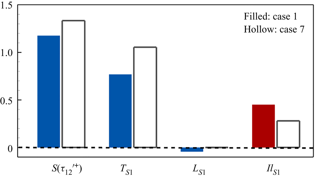
Figure 9 compares the non-zero components of  $S({\tau _{12}}^{\prime +})$ in (4.2) between shallow-water Langmuir turbulence and pure shear-driven turbulence. The small negative value of $L_{S1}$ in figure 9 implies a negatively skewed distribution of $\tau _{12}^{L+}$, i.e. a higher probability for the positive $\tau _{12}^{L+}$ than the negative values. Because $\tau _{12}^{L+}$ is strongly correlated with $u^{L+}$ (figure 5a), the negative skewness of $\tau _{12}^{L+}$ can be explained by the distribution of $u^{L+}$, that is, the positive $u^{L+}$ occupies more than half of the $x$–
$x$– $z$ plane (figures 2 and 3). It is evident from figure 9 that the attenuation of $S({\tau _{12}}^{\prime +})$ in shallow-water Langmuir turbulence is mainly caused by the reduction in $T_{S1}$. Based on its definition given by (4.2) and the definition of the skewness $S({\tau _{12}}^{T+})$, $T_{S1}$ can be rewritten as
 \begin{equation} T_{S1}=\frac{\langle(\tau_{{12}}^{T+})^3\rangle}{\sigma^3({\tau_{12}}^{\prime+})}=\frac{\sigma^3({\tau_{12}}^{T+})}{\sigma^3({\tau_{12}}^{\prime+})} \frac{\langle(\tau_{{12}}^{T+})^3\rangle}{\sigma^3({\tau_{12}}^{T+})}=\frac{\sigma^3({\tau_{12}}^{T+})}{\sigma^3({\tau_{12}}^{\prime+})} S({\tau_{12}}^{T+}). \end{equation}
From the discussion of figure 8,  $\sigma ^3({\tau _{12}}^{T+})/\sigma ^3({\tau _{12}}^{\prime +})$ is known to be smaller in shallow-water Langmuir turbulence than pure shear-driven turbulence owing to the strong linear superimposition effect (figure 8). To study the effect of full-depth LCs on the skewness of $\tau _{{12}}^{T+}$, we decompose $S({\tau _{12}}^{T+})$ into two components as
 \begin{align} S(\tau_{{12}}^{T+}) & =
\frac{\displaystyle\int_{-\infty}^{\infty}
({\tau_{12}}^{T+})^3 P({\tau_{12}}^{T+})
\,\mathrm{d}{\tau_{12}}^{T+}}{\sigma^3({\tau_{12}}^{T+})} \notag \\
& = \frac{\displaystyle\int_{-\infty}^{\infty}
\displaystyle\int^{\infty}_{-\infty} ({\tau_{12}}^{T+})^3
P(u^{L+}, {\tau_{12}}^{T+}) \,\mathrm{d} u^{L+}
\,\mathrm{d}{\tau_{12}}^{T+}}{\sigma^3({\tau_{12}}^{T+})} \nonumber\\
&=\underbrace{\frac{\displaystyle\int_{-\infty}^{\infty}
\displaystyle\int^0_{-\infty} ({\tau_{12}}^{T+})^3
P(u^{L+}, {\tau_{12}}^{T+}) \,\mathrm{d} u^{L+}\,\mathrm{d}
{\tau_{12}}^{T+}}{\sigma^3({\tau_{12}}^{T+})}}_{S_N(\tau_{{12}}^{T+})}
\nonumber\\ &\quad +
\underbrace{\frac{\displaystyle\int_{-\infty}^{\infty}
\displaystyle\int_0^\infty ({\tau_{12}}^{T+})^3 P(u^{L+},
{\tau_{12}}^{T+}) \,\mathrm{d}u^L
\,\mathrm{d}{\tau_{12}}^{T+}}{\sigma^3({\tau_{12}}^{T+})}}_{S_P(\tau_{{12}}^{T+})}.
\end{align}
\begin{align} S(\tau_{{12}}^{T+}) & =
\frac{\displaystyle\int_{-\infty}^{\infty}
({\tau_{12}}^{T+})^3 P({\tau_{12}}^{T+})
\,\mathrm{d}{\tau_{12}}^{T+}}{\sigma^3({\tau_{12}}^{T+})} \notag \\
& = \frac{\displaystyle\int_{-\infty}^{\infty}
\displaystyle\int^{\infty}_{-\infty} ({\tau_{12}}^{T+})^3
P(u^{L+}, {\tau_{12}}^{T+}) \,\mathrm{d} u^{L+}
\,\mathrm{d}{\tau_{12}}^{T+}}{\sigma^3({\tau_{12}}^{T+})} \nonumber\\
&=\underbrace{\frac{\displaystyle\int_{-\infty}^{\infty}
\displaystyle\int^0_{-\infty} ({\tau_{12}}^{T+})^3
P(u^{L+}, {\tau_{12}}^{T+}) \,\mathrm{d} u^{L+}\,\mathrm{d}
{\tau_{12}}^{T+}}{\sigma^3({\tau_{12}}^{T+})}}_{S_N(\tau_{{12}}^{T+})}
\nonumber\\ &\quad +
\underbrace{\frac{\displaystyle\int_{-\infty}^{\infty}
\displaystyle\int_0^\infty ({\tau_{12}}^{T+})^3 P(u^{L+},
{\tau_{12}}^{T+}) \,\mathrm{d}u^L
\,\mathrm{d}{\tau_{12}}^{T+}}{\sigma^3({\tau_{12}}^{T+})}}_{S_P(\tau_{{12}}^{T+})}.
\end{align}
Here, the relationship  $P({\tau _{12}}^{T+}) = \int _{-\infty }^{+\infty } P(u^{L+}, {\tau _{12}}^{T+}) \,\mathrm {d} u^{L+}$ is applied, and the integration is then decomposed into those over positive and negative values of $u^{L+}$, respectively. In (4.4) the subscripts ‘ $N$’ and ‘ $P$’ are used to denote the contributions from the wall shear stress fluctuations under the conditions of $u^{L+}<0$ and $u^{L+}>0$, respectively. Table 2 lists the values of $S({\tau _{12}}^{T+})$, $S_N({\tau _{12}}^{T+})$ and $S_P({\tau _{12}}^{T+})$. As shown, the reduction in $S({\tau _{12}}^{T+})$ in shallow-water Langmuir turbulence is mainly caused by the decrease in $S_N(\tau _{{12}}^{T+})$. This phenomenon is related to the strong suppression effect of full-depth LCs on ${\tau _{12}}^{T+}$ in the region with negative $u^{L+}$, which is the feature of the nonlinear modulation effect of full-depth LCs distinct from that of CCs (figure 5). In summary, full-depth LCs cause the attenuation of $S({\tau _{12}}^{\prime +})$ through the reduction in the contribution proportion of the background turbulence part ${\tau _{12}}^{T+}$ to $\sigma ({\tau _{12}}^{\prime +})$ and the reduction in the skewness of the background turbulence part $S({\tau _{12}}^{T+})$, which are attributed to the strong linear superimposition effect and nonlinear modulation effect, respectively. The impacts of full-depth LCs on ${\tau _{32}}^{\prime +}$ are not investigated, because the skewness of ${\tau _{32}}^{\prime +}$ is zero in both shallow-water Langmuir turbulence and pure shear-driven turbulence.
Skewness of  $\tau _{{12}}^{T+}$ and its components defined by (4.4) in shallow-water Langmuir turbulence (case 1) and pure shear-driven turbulence (case 7).

In the rest of § 4, we discuss the kurtosis  $K(\tau _{{i2}}^{\prime +})$. Figure 10 compares the kurtoses of ${\tau _{12}}^{\prime +}$ and ${\tau _{32}}^{\prime +}$ between shallow-water Langmuir turbulence (case 1) and pure shear-driven turbulence (case 7). It is observed that both $K(\tau _{{12}}^{\prime +})$ and $K(\tau _{{32}}^{\prime +})$ are attenuated in shallow-water Langmuir turbulence, indicating less extreme wall shear stress fluctuations in the presence of full-depth LCs. Similar to the analyses of skewness, the impacts of full-depth LCs on the kurtosis are investigated by decomposing $K(\tau _{{i2}}^{\prime +})$ into
 \begin{align} K(\tau_{{i2}}^{\prime+}) &=\underbrace{\frac{\langle(\tau_{{i2}}^{T+})^4\rangle}{\sigma^4(\tau_{{i2}}^{\prime+})}}_{T_{Ki}} + \underbrace{\frac{\langle(\tau_{{i2}}^{L+})^4\rangle}{\sigma^4(\tau_{{i2}}^{\prime+})}}_{L_{Ki}} + \underbrace{\frac{4 \langle(\tau_{{i2}}^{T+})^3\tau_{{i2}}^{L+}\rangle}{\sigma^4(\tau_{{i2}}^{\prime+})}}_{I1_{Ki}} + \underbrace{\frac{6\langle(\tau_{{i2}}^{T+})^2(\tau_{{i2}}^{L+})^2\rangle}{\sigma^4(\tau_{{i2}}^{\prime+})} }_{I2_{Ki}}\nonumber\\ &\quad + \underbrace{\frac{4\langle\tau_{{i2}}^{T+}(\tau_{{i2}}^{L+})^3\rangle}{\sigma^4(\tau_{{i2}}^{\prime+})}}_{I3_{Ki}}, \quad i=1\ \mathrm{or}\ {3}, \end{align}
based on the triple decomposition (2.7) and the definition of the kurtosis. The components  $T_{Ki}$ and $L_{Ki}$ represent the contributions from the background turbulence and full-depth LCs, respectively. The other three terms represent the contributions of the nonlinear interaction between the background turbulence and full-depth LCs, among which $I3_{Ki}$ is trivial according to the definition of the triple decomposition given by (2.4). The non-zero components of $K(\tau _{{i2}}^{\prime +})$ in (4.5) are compared between shallow-water Langmuir turbulence and pure shear-driven turbulence in figure 10. For both ${\tau _{12}}^{\prime +}$ and ${\tau _{32}}^{\prime +}$, the reduction in their kurtoses in the presence of full-depth LCs stems from the attenuation of $T_{Ki}$.
Comparison of the kurtosis components of (a)  $\tau _{{12}}^{\prime +}$ and (b) $\tau _{{32}}^{\prime +}$ in (4.5) between shallow-water Langmuir turbulence (case 1) and pure shear-driven turbulence (case 7). The red and blue coloured bars indicate an increase and reduction in the values in case 1 compared with those in case 7, respectively.

Based on the expression of  $T_{Ki}$ in (4.5) and the definition of $K(\tau _{{i2}}^{T+})$, we derive that $T_{Ki}$ equals the multiplication of $\sigma ^4(\tau _{{i2}}^{T+})/ \sigma ^4 (\tau _{{i2}}^{\prime +})$ and $K(\tau _{{i2}}^{T+})$. As shown in figure 8, the linear superimposition effect of full-depth LCs leads to the reduction in $\sigma ^4(\tau _{{i2}}^{T+})/ \sigma ^4 (\tau _{{i2}}^{\prime +})$. Meanwhile, as shown in table 3, $K(\tau _{{i2}}^{T+})$ also reduces in shallow-water Langmuir turbulence. The reduction in $K(\tau _{{i2}}^{T+})$ suggests that the events of extreme $\tau _{{i2}}^{T+}$ diminish in the presence of full-depth LCs, which is related to the strong suppression effect of negative $u^{L+}$ on $\tau _{{i2}}^{T+}$. To demonstrate this point, $K(\tau _{{i2}}^{T+})$ is decomposed into $K_N(\tau _{{i2}}^{T+})$ and $K_P(\tau _{{i2}}^{T+})$ conditioned upon the negative and positive $u^{L+}$, respectively,
 \begin{align} K(\tau_{{i2}}^{T+}) &= \underbrace{\frac{\displaystyle\int_{-\infty}^{\infty} \displaystyle\int^0_{-\infty} (\tau_{{i2}}^{T+})^4 P(u^{L+}, \tau_{{i2}}^{T+}) \,\mathrm{d} u^{L+}\,\mathrm{d}\tau_{{i2}}^{T+}}{\sigma^4(\tau_{{i2}}^{T+})}}_{K_N(\tau_{{i2}}^{T +})} \nonumber\\ &\quad + \underbrace{\frac{\displaystyle\int_{-\infty}^{\infty} \displaystyle\int_0^\infty (\tau_{{i2}}^{T+})^4 P(u^{L+}, \tau_{{i2}}^{T+}) \,\mathrm{d} u^{L+} \,\mathrm{d}\tau_{{i2}}^{T+}}{\sigma^4(\tau_{{i2}}^{T+})}}_{K_P(\tau_{{i2}}^{T+})}, \end{align}
which is similar to the decomposition in (4.4). Table 3 compares the values of  $K_N(\tau _{{i2}}^{T+})$ and $K_P(\tau _{{i2}}^{T+})$ between shallow-water Langmuir turbulence and pure shear-driven turbulence. The values of $K_P({\tau _{12}}^{T+})$ are close to each other in these two flows, while the values of $K_N({\tau _{12}}^{T+})$ are notably smaller in the presence of full-depth LCs owing to the stronger suppression of $\tau _{{i2}}^{T+}$ by full-depth LCs in the region with negative $u^{L+}$ (figure 5). Therefore, it is the linear superimposition effect and nonlinear modulation effect of full-depth LCs that are responsible for the reduction in the probability of extreme wall shear stress fluctuations.
Kurtosis of  $\tau _{{i2}}^{T+}$ and its components defined by (4.6) in shallow-water Langmuir turbulence (case 1) and pure shear-driven turbulence (case 7).
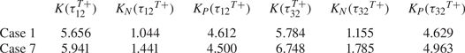
The above analyses address the second question raised in § 1. Our results indicate that the strong linear superimposition effect of full-depth LCs on the wall shear stress fluctuations enhances their mean square value, while the combination of the strong nonlinear modulation effect and linear superimposition effect of full-depth LCs suppresses their skewness and kurtosis. From the analyses in this section and in § 3, we conclude that the dual effects of full-depth LCs on wall shear stress fluctuations are important for both their spatial distributions and statistics. Next in § 5, scaling analyses of the dual effects are performed to develop a predictive model for the wall shear stress fluctuations in shallow-water Langmuir turbulence.
5. Scaling and modelling of wall shear stress fluctuations
This section aims to develop a predictive model for the streamwise and spanwise wall shear stress fluctuations in shallow-water Langmuir turbulence. Predictive models for the LCs part and background turbulence part of wall shear stress fluctuations are first developed based on the scalings of the linear superimposition effect and nonlinear modulation effect of full-depth LCs, respectively. Then, the predictive model of wall shear stress fluctuations is assessed using cases 1–6. At last, the effects of LCs at low turbulent Langmuir number and high wavenumber of water waves in cases 8 and 9 are studied.
5.1. Scaling and predictive model of LCs part
As analysed in § 3.2, the LCs part of wall shear stress fluctuations  $\tau _{{i2}}^{L+}$ varies linearly with the LCs part of velocity $u_i^{L+}$ at $y/h=0.1$ in shallow-water Langmuir turbulence (see figures 5 and 7). To confirm this linear relationship for $u_i^{L+}$ at other $y/h$ and under various flow conditions, we examine the correlation coefficient between $u_i^{L+} (y, z, t)$ and $\tau _{{i2}}^{L+}(z, t)$ in cases 1–6, which is defined as
 \begin{equation} C_{u_i^L, \tau_{{i2}}^L}(y) = \frac{\langle u_i^{L+}(y,z,t) \tau_{{i2}}^{L+}(z,t) \rangle}{\sqrt{\langle (u_i^{L+}(y,z,t) )^2 \rangle}\sqrt{\langle (\tau_{{i2}}^{L+}(z,t))^2 \rangle}},\quad i= 1\ \text{or}\ 3. \end{equation}
Figure 11 shows the vertical profiles of  $C_{u^L, {\tau _{12}}^L}(y)$ and $C_{w^L, {\tau _{32}}^L}(y)$. As shown, in the bottom quarter of the water column ( $0< y/h<0.5$), $C_{u^{L},{\tau _{12}}^{L}}$ and $C_{w^{L},{\tau _{32}}^{L}}$ are larger than $0.8$ in all cases with full-depth LCs (cases 1–6 in table 1). The high correlation coefficients in shallow-water Langmuir turbulence suggest that a linear function of $u_i^{L+}$ can approximately estimate $\tau _{{i2}}^{L+}$, viz.
 \begin{equation} \tau_{{i2}}^{L+}(z, t) \approx \alpha_i(y)u_i^{L+}(y,z,t),\quad i=1 \text{or}\ 3. \end{equation}
Profiles of (a)  $C_{u^L,{\tau _{12}}^L}$ and (b) $C_{w^L,{\tau _{32}}^L}$ in shallow-water Langmuir turbulence under various flow conditions (cases 1–6 listed in table 1).

The coefficient  $\alpha _i(y)$ can be calculated using the linear stochastic approximation method as
 \begin{equation} \alpha_i(y)=C_{u_i^{L}, \tau_{{i2}}^{L}}(y)\frac{\sqrt{\langle (\tau_{{i2}}^{L+}(z,t) )^2 \rangle}}{\sqrt{\langle (u_i^{L+}(y,z,t) )^2 \rangle}}. \end{equation}
Figure 12 shows the profiles of  $\alpha _1(y)$ and $\alpha _3(y)$ in cases 1–6 for $0< y/h<0.5$. The discrepancy of $\alpha _i(y)$ among different cases is marginal. Therefore, the LCs part of wall shear stress fluctuations $\tau _{{i2}}^{L+}$ can be scaled and predicted by the LCs part of the velocity $u_i^{L+}$ measured in the bottom quarter of the water column.


Because full-depth LCs are uniform in the streamwise direction and well organized in the spanwise direction,  $\tau _{i2}^L$ can also be predicted by the velocity $u_i^L$ at a different spanwise location. To confirm this, the two-point correlation coefficient $C_{u_i^L, \tau _{{i2}}^L}(y,\Delta z)$, defined as
 \begin{equation} C_{u_i^L, \tau_{{i2}}^L}(y,\Delta z) = \frac{\langle u_i^{L+}(y,z+\Delta z,t) \tau_{{i2}}^{L+}(z,t) \rangle}{\sqrt{\langle (u_i^{L+}(y,z,t) )^2 \rangle}\sqrt{\langle (\tau_{{i2}}^{L+}(z,t))^2 \rangle}},\quad i= 1\ \text{or}\ 3, \end{equation}
is studied. Figures 13(a) and 13(b) display the distribution of  $C_{u_i^L, \tau _{{i2}}^L}(y,\Delta t)$ in case 1 as an example. The results in cases 2–6 are similar. As shown, $C_{u_i^L, \tau _{{i2}}^L}(y,\Delta t)$ is larger than 0.8 for $-0.5<\Delta z/h<0.5$. Additionally, the corresponding linear coefficients $\alpha _i(y,\Delta z)$, defined similar to (5.3), show insignificant variation for $-0.5<\Delta z/h<0.5$ (figure 13c,d). Therefore, the velocity $u_{i}^{L}(y,z+\Delta z, t)$ with $-0.5<\Delta z/h<0.5$ can be used in (5.2), indicating that the velocity $u_{i}^{L}$ at a specific location in the outer layer can provide more predictive values.
Contours of (a,b) the two-point spatial correlation coefficient  $C_{u_i^L, \tau _{{i2}}^L}(y,\Delta z)$ and (c,d) the linear coefficients $\alpha _i(y,\Delta z)$ in case 1. In (a,c) $i=1$, and in (b,d) $i=3$. In (a,b) the solid and dashed black lines indicate $C_{u_i^L, \tau _{{i2}}^L}(y,\Delta z)=0.8$ and $=-0.8$, respectively.

In wall turbulence without waves, there is a time delay between LSMs and the wall shear stresses owing to the propagation of the information from the outer layer to the bottom (Mathis et al. Reference Mathis, Marusic, Chernyshenko and Hutchins2013; Scherer et al. Reference Scherer, Uhlmann, Kidanemariam and Krayer2022). We also explore the time delay based on the spatial–temporal correlation coefficient, defined as
 \begin{equation} C_{u_i^L, \tau_{{i2}}^L}(y,\Delta t) = \frac{\langle u_i^{L+}(y,z,t+\Delta t) \tau_{{i2}}^{L+}(z,t) \rangle}{\sqrt{\langle (u_i^{L+}(y,z,t) )^2 \rangle}\sqrt{\langle (\tau_{{i2}}^{L+}(z,t))^2 \rangle}},\quad i= 1\ \text{or}\ 3, \end{equation}
in shallow-water Langmuir turbulence. Figure 14 displays  $C_{u_i^L, \tau _{{i2}}^L}(y,\Delta t)$ in case 1. There exists a ridge in the contours of $C_{u_i^L, \tau _{{i2}}^L}(y,\Delta t)$ with a negative slope, indicating that $\tau _{i2}^L$ is induced by a top–down mechanism of $u_i^{L}$ similar to the finding of Scherer et al. (Reference Scherer, Uhlmann, Kidanemariam and Krayer2022) in open channel flow without waves. However, compared with the rapid decline of the spatial–temporal correlation found in the open channel (Scherer et al. Reference Scherer, Uhlmann, Kidanemariam and Krayer2022), the spatial–temporal correlation coefficients in figure 14 are larger than $0.8$ for $-2<\Delta t u_w/h<2$ and $0< y/h<0.5$. This result is consistent with the observation in the works of Shrestha & Anderson (Reference Shrestha and Anderson2020) and Deng et al. (Reference Deng, Yang, Xuan and Shen2020), that is, the intensities and spanwise locations of full-depth LCs are persistent for a period of $100< tu_w/h<300$. Therefore, the velocity $u_i^{L}$ at $(y, z, t+\Delta t)$ can also be used to predict the wall shear stress $\tau _{i2}^L$ at $(z,t)$ for $0< y/h<0.5$ and $-2<\Delta t u_w/h<2$.
Contours of the spatial–temporal correlation coefficient  $C_{u_i^L, \tau _{{i2}}^L}(y,\Delta t)$ in case 1. In (a,b) $i=1$ and $3$, respectively. The black dashed lines represent the ridges of the contours.

In canonical wall turbulence the large-scale streamwise velocity and streamwise wall shear stress fluctuation also satisfy a linear relationship (Mathis et al. Reference Mathis, Marusic, Chernyshenko and Hutchins2013). The value of the linear coefficient found in canonical wall turbulence at  $y^+=3.9\sqrt {Re_\tau }$ is 0.0898 (Mathis et al. Reference Mathis, Marusic, Chernyshenko and Hutchins2013), close to $\alpha _1$ at $y/h=0.1$, which is approximately 0.0845, in shallow-water Langmuir turbulence (figure 12a). However, full-depth LCs induce stronger streamwise velocity than LSMs (Deng et al. Reference Deng, Yang, Xuan and Shen2019). Consequently, full-depth LCs impose a more significant linear superimposition effect on the wall shear stress fluctuations than LSMs, which is partially responsible for the distinct spatial patterns of wall shear stress fluctuations in shallow-water Langmuir turbulence depicted in figure 3.
5.2. Scaling and predictive model of the background turbulence part
In this section we derive a predictive model for the background turbulence part of wall shear stress fluctuations  $\tau _{{i2}}^{T+}$ based on the scaling of the nonlinear modulation effect of full-depth LCs on $\tau _{{i2}}^{T+}$ and the properties of the demodulated counterpart of $\tau _{{i2}}^{T+}$. Furthermore, the predictive model is utilized to quantitatively measure the impacts of the LCs part of the streamwise velocity $u^{L+}$ on the statistics of $\tau _{{i2}}^{T+}$, which is an important component of the statistics of the wall shear stress fluctuations $\tau _{{i2}}^{\prime +}$.
5.2.1. Scaling of the nonlinear modulation effect of LCs
As analysed in § 3.2, the background turbulence part of wall shear stress fluctuations,  $\tau _{{i2}}^T$, is modulated by the LCs part of streamwise velocity fluctuations, $u^{L}$, which shows an organized spanwise variation. Therefore, the modulation effect of full-depth LCs on $\tau _{{i2}}^T$ can be measured by the correlation between $u^{L+}$ and the spanwise variation of the magnitude of $\tau _{{i2}}^{T+}$. The latter can be quantified using a function defined as
 \begin{equation} f_i(z,t)=\frac{(\tau_{{i2}}^{T})_{x,rms}^+(z,t)-(\tau_{{i2}}^{T})_{rms}^+} {(\tau_{{i2}}^{T})_{rms}^+}, \end{equation}
where the subscript ‘ ${x,rms}$’ indicates the localized r.m.s. value based on streamwise averaging.
For  ${\tau _{12}}^T$, the relationship between its spanwise variation $f_1(z,t)$ defined above and $u^{L+}$ can be derived analytically using the scaling of the localized r.m.s. value of the background turbulence part of streamwise velocity $u^{T+}$ obtained by Deng et al. (Reference Deng, Yang, Xuan and Shen2020). Based on the definition of wall shear stress (2.6) and the no-slip boundary condition, $\tau _{{i2}}^{T+}$ and $u_i^{T+}$ satisfy the following relationship:
 \begin{equation} \tau_{{i2}}^{T+} (x,z,t) =\lim_{\delta y^+\rightarrow 0} \frac{u_i^{T+}(x,\delta y^+,z,t)}{\delta y^+}\approx \frac{u_i^{T+}(x,\delta y^+,z,t)}{\delta y^+}. \end{equation}
Here  $\delta y^+$ is a small distance from the water bottom. Therefore, the r.m.s. value and localized r.m.s. value of $\tau _{{i2}}^{T+}$ in (5.6) can be approximated as
 \begin{equation} (\tau_{{i2}}^{T})_{rms}^+{\approx} \frac{(u_i^T)_{rms}^+(\delta y^+)}{\delta y^+} \end{equation}
and
 \begin{equation} (\tau_{{i2}}^{T})_{x,rms}^+ (z,t) \approx \frac{(u_i^T)_{x,rms}^+(\delta y^+,z,t)}{\delta y^+}, \end{equation}
respectively. As found in Deng et al. (Reference Deng, Yang, Xuan and Shen2020), the vertical profile of  $(u^T)_{xt,rms}^+$ is well scaled by a localized friction velocity $u_l$ in a localized vertical coordinate $y^l=yu_l/\nu$, collapsing into the profile of $(u^T)_{rms}^+$ in the vertical coordinate $y^+$, viz.
 \begin{equation} \frac{(u^T)_{xt,rms}}{u_l} \left(\frac{y\nu} {u_l}, z \right ) = \frac{(u^T)_{rms}}{u_w} \left(\frac{y\nu}{u_w}\right). \end{equation}
Here, the subscript ‘ $xt$’ indicates the streamwise and time averaging. The localized friction velocity $u_l$ is defined as
 \begin{equation} u_l = \sqrt{\nu \frac{\partial(\langle u \rangle + \langle u^L \rangle_{t})}{\partial y}}\approx\sqrt{\nu \frac{\partial(\langle u \rangle + u^L)}{\partial y}}= u_w\sqrt{1 + {\tau_{12}}^{L+}}, \end{equation}
where the subscript ‘ $t$’ represents the time averaging and the relationship $\langle u^L\rangle _t(y,z)\approx u^L(y,z,t)$ found in Deng et al. (Reference Deng, Yang, Xuan and Shen2020) is applied. Additionally, $(u^T)_{x,rms}=(u^T)_{xt,rms}$ approximately holds at an equilibrium state. According to this relationship and (5.10), the term $(u^T)_{x,rms}^+(\delta y^+,z)$ in (5.9) is approximately
 \begin{equation} (u^T)^+_{x,rms} (\delta y^+,z,t) \approx \frac{u_l}{u_w} (u^T)^+_{rms} \left(\frac{\delta y^+ u_l}{u_w}\right). \end{equation}
Substituting (5.12) into (5.9), and then using the relationships in (5.8) and (5.11), we can derive that
 \begin{equation} (\tau_{{12}}^{T})_{x,rms}^+{\approx} \frac{u_l^2}{u_w^2}\dfrac{(u^T)_{rms}^+\left(\dfrac{u_l\delta y^+}{u_w}\right)}{\dfrac{u_l\delta y^+}{u_w}}\approx\dfrac{u_l^2}{u_w^2}(\tau_{{12}}^{T})_{rms}^+{\approx}(1+ {\tau_{12}}^{L+})(\tau_{{12}}^{T})_{rms}^+. \end{equation}
Further substituting (5.13) into (5.6), and applying the linear relationship between  $u^{L+}$ and ${\tau _{12}}^{L+}$ in (5.2), $f_1$ can be approximated as
 \begin{equation} f_1\approx \alpha_1 u^{L+}, \end{equation}
where  $\alpha _1$ is given in (5.2).
For  $(w^{T})_{xt,rms}$, because a simple scaling in a form similar to (5.10) has not yet been discovered (Deng et al. Reference Deng, Yang, Xuan and Shen2020), it is necessary to scale the modulation effect of full-depth LCs on ${\tau _{32}}^{T+}$ by computing the correlation coefficient between $f_3$ and $u^{L+}$, defined as
 \begin{equation} C_{u^{L},f_3}=\frac{\langle u^{L+}f_3 \rangle}{\sqrt{\langle (u^{L+})^2 \rangle}\sqrt{\langle (f_3)^2 \rangle}}. \end{equation}
As shown in figure 15(a), except for the lowest Reynolds number  $Re_\tau =395$ (case 3), $C_{u^{L},f_3}$ in the other cases is larger than 0.8 in the bottom quarter of the water column. The high correlation coefficients suggest that at moderate to high Reynolds numbers, $f_3$ may be approximated by a linear function of $u^{L+}$ as
 \begin{equation} f_3\approx\beta_3 u^{L+}. \end{equation}
The parameter  $\beta _3$ is determined by the linear stochastic estimation method as
 \begin{equation} \beta_3 (y) =C_{u^{L},f_3}\frac{\sqrt{\langle (f_3)^2 \rangle}}{\sqrt{\langle (u^{L+})^2 \rangle}}. \end{equation}
As shown in figure 15(b),  $\beta _3$ is insensitive to the wavenumber of water waves, turbulent Langmuir number and Reynolds number for cases with $Re_\tau \geqslant 700$ considered in the present study.
Profiles of (a)  $C_{u^L,f_3}$ and (b) $\beta _3$ in shallow-water Langmuir turbulence under various flow conditions (cases 1–6 listed in table 1).

The relationships given by (5.14) and (5.16) are equivalent to
 \begin{equation} (\tau_{{i2}}^{T})_{x,rms}^+ (z,t)\approx(\tau_{{i2}}^{T})_{rms}^+(1+\beta_i (y) u^{L+} (y,z,t)), \end{equation}
which explicitly measure the nonlinear modulation effect of  $u^{L+}$ on the magnitude of $\tau _{{i2}}^{T+}$ at different spanwise locations. Here, $1+\beta _iu^{L+}$ represents the modulation degree, and $\beta _i$ is the modulation coefficient with $\beta _1=\alpha _1$ and $\beta _3$ given by (5.17). Because the value of $\beta _i$ is similar among the various cases (except for case 3, which has the lowest Reynolds number $Re_\tau =395$) as shown previously in figures 12(a) and 15(b), the modulation degree reduces to be related to $u^{L+}$, which varies with the Reynolds number, wavenumber of surface waves and turbulent Langmuir number (Tejada-Martínez & Grosch Reference Tejada-Martínez and Grosch2007; Sinha et al. Reference Sinha, Tejada-Martínez, Akan and Grosch2015; Deng et al. Reference Deng, Yang, Xuan and Shen2019).
The modulation coefficient  $\beta _1$ is close to that in canonical wall turbulence (Mathis et al. Reference Mathis, Marusic, Chernyshenko and Hutchins2013). Because of the larger magnitude of $u^{L+}$ in shallow-water Langmuir turbulence compared with the large-scale streamwise velocity in canonical wall turbulence, the modulation effect of full-depth LCs on ${\tau _{12}}^{T+}$ is more significant. In canonical wall turbulence the modulation effects of large-scale streamwise velocity on spanwise wall shear stress fluctuations have not been reported in the literature. In shallow-water Langmuir turbulence the modulation effect of full-depth LCs on ${\tau _{32}}^{T+}$ is evident, although it is slightly weaker than that on ${\tau _{12}}^{T+}$ because $\beta _3<\beta _1$.
5.2.2. Predictive model of the background turbulence part
According to the nonlinear modulation effect of full-depth LCs on the background turbulence part of wall shear stress fluctuations described by (5.18), we approximate  $\tau _{{i2}}^{T+}$ as
 \begin{equation} \tau_{{i2}}^{T+} \approx(1+\beta_iu^{L+})\tau_{{i2}}^{{\ast}{+}}. \end{equation}
Here,  $\tau _{{i2}}^{\ast +}$ is the demodulated counterpart of $\tau _{{i2}}^{T+}$ calculated by
 \begin{equation} \tau_{{i2}}^{{\ast}{+}} = \frac{\tau_{{i2}}^{T+}}{1 + \beta_i u^{L+}}. \end{equation}
It can be verified, by using (5.20) and (5.18), that the correlation coefficient between  $u^{L+}$ and the spanwise variation of the magnitude of $\tau _{{i2}}^{\ast +}$ (which is similar to that of $\tau _{{i2}}^{T+}$ defined in (5.6)) is near zero, indicating the absence of the nonlinear modulation effect of full-depth LCs on $\tau _{{i2}}^{\ast +}$. This result is also confirmed by the instantaneous fields of ${\tau _{12}}^{\ast +}$ and ${\tau _{32}}^{\ast +}$ plotted in figures 16(a) and 17(a), respectively. As shown, they exhibit homogeneous distributions in the $x$–
$x$– $z$ plane without obvious nonlinear modulation by full-depth LCs.
Properties of the demodulated background turbulence part of wall shear stress fluctuation  $\tau _{{12}}^{\ast +}$. (a) Instantaneous field of $\tau _{{12}}^{\ast +}$ obtained from case 1. (b) Probability density function of $\bar {\tau }_{{12}}^{\ast }$. (c) Variation of the r.m.s. values of $\tau _{{12}}^{\ast +}$ with the Reynolds number under different flow conditions (cases 1–6). The black line represents the logarithmic variation of $(\tau _{{12}}^{\ast })_{rms}^+$ with the Reynolds number.

The properties of  $\tau _{{i2}}^{\ast +}$ are essential for the application of the predictive model. To illustrate this, we plot the statistics of $\tau _{{i2}}^{\ast +}$ in figures 16 and 17. As shown in figures 16(b) and 17(b), the probability density functions of the normalized $\tau _{{i2}}^{*+}$, defined as $\bar {\tau }_{i2}^{\ast }=\tau _{{i2}}^{\ast }/(\tau _{{i2}}^{\ast })_{rms}$, of different cases collapse into one curve, indicating that $\bar {\tau }_{i2}^{\ast }$ is independent of the Reynolds number (cases 1–3), wavenumber of surface waves (cases 1, 4 and 5), and turbulent Langmuir number (cases 1 and 6) considered in this study. Therefore, we approximate the instantaneous field of $\tau _{{i2}}^{\ast +}$ using the product of $(\tau _{{i2}}^{*})_{rms}^{+}$ in different cases and $\bar {\tau }_{i2}^{\ast }$ from case 1 (figures 16a, 17a), viz.
 \begin{equation} \tau_{{i2}}^{{\ast}{+}} = (\tau_{{i2}}^{{\ast}})_{rms}^{+}\bar{\tau}_{i}^{*}. \end{equation}
Properties of the demodulated background turbulence part of wall shear stress fluctuation  $\tau _{{32}}^{\ast +}$. (a) Instantaneous field of $\tau _{{32}}^{\ast +}$ obtained from case 1. (b) Probability density function of $\bar {\tau }_{{32}}^{\ast }$. (c) Variation of the r.m.s. values of $\tau _{{32}}^{\ast +}$ with the Reynolds number under different conditions (cases 1–6). The black line represents the logarithmic variation of $(\tau _{{32}}^{\ast })_{rms}^+$ with the Reynolds number.

Computing the r.m.s. values of the terms on the two sides of (5.19) and then using the relationship in (5.8) results in
 \begin{equation} (\tau_{{i2}}^{{\ast}})_{rms}^{+} =\frac{(\tau_{{i2}}^{T})_{rms}^+}{ \sqrt{1+\beta_i^2 \left((u^{L})_{rms}^+\right)^{2}}}\approx\frac{(u_i^T)_{rms}^+(\delta y^+)}{\sqrt{1+\beta_i^2 \left((u^{L})_{rms}^+\right)^{2}} \delta y^+}. \end{equation}
As reported by Sinha et al. (Reference Sinha, Tejada-Martínez, Akan and Grosch2015) and Deng et al. (Reference Deng, Yang, Xuan and Shen2019), the values of  $(u^T)_{rms}^+$ and $(w^T)_{rms}^+$ near the bottom increase slightly with the turbulent Langmuir number and wavenumber of water waves but grow noticeably with the Reynolds number. As a result, $(\tau _{{i2}}^{\ast })_{rms}^{+}$ in shallow-water Langmuir turbulence responses to the three non-dimensional parameters following the response of the near-bottom $(u^T)_{rms}^+$ and $(w^T)_{rms}^+$ (figures 16c and 17c). Ignoring the tiny variation of $(\tau _{{i2}}^{\ast })_{rms}^{+}$ with the turbulent Langmuir number and wavenumber, the values of $({\tau _{12}}^{\ast })_{rms}^{+}$ and $({\tau _{32}}^{\ast })_{rms}^{+}$ in different cases approximately satisfy logarithmic laws of the Reynolds number denoted in figures 16(c) and 17(c), respectively. The logarithmic variation may be attributed to LSMs in the background turbulence part of shallow-water Langmuir turbulence. In canonical wall turbulence, LSMs lead to a logarithmic variation of the r.m.s. value of streamwise wall shear stress fluctuations with the Reynolds number (Örlü & Schlatter Reference Örlü and Schlatter2011).
Finally, substituting (5.21) into (5.19),  $\tau _{{i2}}^{T+}$ can be predicted as
 \begin{equation} \tau_{{i2}}^{T+} = (1 + \beta_i u^{L+})(\tau_{{i2}}^{*})_{rms}^+\bar{\tau}_{i}^{*}. \end{equation}
In this predictive model the value of  $(\tau _{{i2}}^{*})_{rms}^+$ can be approximated using the logarithmic laws (figures 16c and 17c). The terms $\beta _i$ and $\bar {\tau }_{i}^{*}$ are almost constant in the various cases of full-depth LCs and can thus be approximated using those obtained from case 1. Therefore, $\tau _{{i2}}^{T+}$ can be reconstructed using $u^{L+}$ measured in the bottom quarter of the water column.
5.2.3. Scaling of skewness and kurtosis of background turbulence part of wall shear stress
As analysed in § 3.2, the nonlinear modulation effect of full-depth LCs can alter the skewness and kurtosis of the background turbulence part of wall shear stresses. In the following, we use the predictive model in (5.23) to explicitly quantify this effect.
The skewness and kurtosis of  $\tau _{{i2}}^{T+}$ can be calculated based on their definitions as
 \begin{align} S(\tau_{{i2}}^{T+})=\frac{\left \langle (\tau_{{i2}}^{T+})^3 \right \rangle}{\left((\tau_{{i2}}^{T})^+_{rms}\right)^{3}}=\frac{\displaystyle\int (\tau_{{i2}}^{T+})^3P(\tau_{{i2}}^{T+}) \,\mathrm{d}\tau_{{i2}}^{T+}}{\left((\tau_{{i2}}^{T})^+_{rms}\right)^{3}}=\frac{\displaystyle\int\int (\tau_{{i2}}^{T+})^3P(u^{L+},\tau_{{i2}}^{T+}) \,\mathrm{d}u^{L+} \,\mathrm{d}\tau_{{i2}}^{T+}}{\left((\tau_{{i2}}^{T})^+_{rms}\right)^{3}} \end{align}
and
 \begin{align} K(\tau_{{i2}}^{T+})=\frac{\left \langle (\tau_{{i2}}^{T+})^4 \right \rangle}{\left((\tau_{{i2}}^{T})^+_{rms}\right)^{4}}=\frac{\displaystyle\int (\tau_{{i2}}^{T+})^4P(\tau_{{i2}}^{T+})\,\mathrm{d}\tau_{{i2}}^{T+}}{\left((\tau_{{i2}}^{T})^+_{rms}\right)^{4}}=\frac{\displaystyle\int\int (\tau_{{i2}}^{T+})^4 P(u^{L+},\tau_{{i2}}^{T+}) \,\mathrm{d}u^{L+} \mathrm{d}\tau_{{i2}}^{T+}}{\left((\tau_{{i2}}^{T})^+_{rms}\right)^{4}}, \end{align}
respectively.
According to the Jacobi transformation of the j.p.d.f. and the predictive model in (5.23), the j.p.d.f.  $P(u^{L}, \tau _{{i2}}^{T})$ can be written as
 \begin{equation} P(u^{L+}, \tau_{{i2}}^{T+})=\frac{P\left(u^{L+}, \bar{\tau}_{i2}^{{\ast}}=\dfrac{\tau_{{i2}}^{T+}}{(\tau_{{i2}}^{*})_{rms}^+(1+\beta_iu^{L+})}\right)}{(\tau_{{i2}}^{*})_{rms}^+(1+\beta_iu^{L+})}. \end{equation}
Because  $u_i^{L}$ and $\bar {\tau }_{i}^{\ast }$ are independent of each other, the identity $P(u^{L}, \bar {\tau }_{i2}^{\ast })=P(u^{L})P(\bar {\tau }_{i2}^{\ast })$ holds. Thus, the j.p.d.f. $P(u^{L}, \tau _{{i2}}^{T})$ can be further expressed as
 \begin{equation} P(u^{L+}, \tau_{{i2}}^{T+})=\frac{P(u^{L+}) P\left( \bar{\tau}_{i2}^{{\ast}}=\dfrac{\tau_{{i2}}^{T+}}{(\tau_{{i2}}^{*})_{rms}^+(1+\beta_iu^{L+})}\right)}{(\tau_{{i2}}^{*})_{rms}^+(1+\beta_iu^{L+})}. \end{equation}
 Substituting (5.23), (5.27) and the identity  $\mathrm {d}u^{L+}\,\mathrm {d}\tau _{{i2}}^{T+}=(\tau _{{i2}}^{*})_{rms}^+(1+\beta _iu^{L+})\,\mathrm {d}u^{L+} \,\mathrm {d}\bar {\tau }_i^{\ast }$ into (5.24) and (5.25), we obtain
 \begin{equation} S(\tau_{{i2}}^{T+})=S(\bar{\tau}_{i2}^{{\ast}})\frac{\langle(1+\beta_iu^{L+})^3\rangle}{(\sqrt{\langle( 1+\beta_i u^{L+})^2\rangle})^3} \end{equation}
and
 \begin{equation} K(\tau_{{i2}}^{T+})=K(\bar{\tau}_{i2}^{{\ast}})\frac{\langle(1+\beta_i u^{L+})^4\rangle}{(\sqrt{\langle( 1+\beta_i u^{L+})^2\rangle})^4}. \end{equation}
Because  $P(\bar {\tau }_{i2}^{\ast })$ is almost the same among different cases (figures 16b and 17b), $S(\bar {\tau }_{i2}^{\ast })$ and $K(\bar {\tau }_{i2}^{\ast })$ are insensitive to the Reynolds number ( $Re_\tau$), wavenumber of surface waves ( $kh$) and turbulent Langmuir number ( $La_t$). Therefore, the variations of $S(\tau _{{i2}}^{T+})$ and $K(\tau _{{i2}}^{T+})$ under different flow conditions are only determined by the statistics of $1+\beta _i u^{L+}$, which represents the modulation degree of full-depth LCs on $\tau _{{i2}}^{T+}$ in (5.23).
The above scaling models can be used to predict the response of  $S(\tau _{{i2}}^{T+})$ and $K(\tau _{{i2}}^{T+})$ to $u^{L+}$ in shallow-water Langmuir turbulence. Figure 18 compares the values of $S(\tau _{{i2}}^{T+})$ and $K(\tau _{{i2}}^{T+})$ obtained from the LES results with the predictions $S(\tau _{i2p}^{T+})$ and $K(\tau _{i2p}^{T+})$ calculated by (5.28) and (5.29), respectively, where $u^{L+}$ is taken at $y/h=0.1$ ( $y^+=100$ for cases 1 and 4–6, $y^+=70$ for case 2, and $y^+=39.5$ for case 1). As shown, the scaling models given by (5.28) and (5.29) can satisfactorily predict the values of $S(\tau _{{i2}}^{T+})$ and $K(\tau _{{i2}}^{T+})$. As $Re_\tau$ decreases (compare cases 1–3), $kh$ increases (compare cases 1, 4 and 5), or $La_t$ increases (compare cases 1 and 6), $S(\tau _{{i2}}^{T+})$ and $K(\tau _{{i2}}^{T+})$ increase, while the magnitude of $1+\beta _i u^{L+}$ in the scaling models (5.28) and (5.29) decreases owing to the reduction in the magnitude of $u^{L+}$(Deng et al. Reference Deng, Yang, Xuan and Shen2019). As a result, $S(\tau _{{i2}}^{T+})$ and $K(\tau _{{i2}}^{T+})$ increase as the modulation degree of full-depth LCs scaled by $1+\beta _i u^{L+}$ decreases.
Comparison of the skewness and kurtosis of  $\tau _{{i2}}^{T+}$ obtained from LES with those predicted by (5.28)–(5.29) using $u^{L+}$ taken at the height $y/h=0.1$ ( $y^+=100$ for cases 1 and 4–6, $y^+=70$ for case 2, and $y^+=39.5$ for case 1). (a) Skewness of ${\tau _{12}}^{T+}$. (b) Kurtosis of ${\tau _{12}}^{T+}$. (c) Kurtosis of ${\tau _{32}}^{T+}$.

5.3. Assessment of predictive modelling
Based on the predictive models of the LCs part and background turbulence part of wall shear stress fluctuations in (5.2) and (5.23), respectively, the total wall shear stress fluctuations  $\tau _{{i2}}^{\prime +}$ can now be predicted by
 \begin{equation} \tau_{ip}^{\prime +} =\alpha_i u_i^{L+} + (1 + \beta_i u^{L+})(\tau_{{i2}}^{*})_{rms}^+\bar{\tau}_{i}^{*}. \end{equation}
 Figure 19 displays an instantaneous field of  $\tau _{{i2}}^{\prime +}$ predicted by (5.30) using $u^{L+}$ and $w^{L+}$ at $y/h=0.1$ ( $y^+=100$ in case 1). The prediction reproduces the organized spanwise variation of wall shear stress fluctuations shown in figure 3. We found that the correlation coefficient between the predicted field and real field is 0.98 for ${\tau _{12}}^{\prime +}$ and 0.96 for ${\tau _{32}}^{\prime +}$, confirming the accuracy of (5.30) in predicting the spatial patterns of wall shear stress fluctuations in shallow-water Langmuir turbulence. The predictive model can be further validated qualitatively by comparing the predicted statistics with the LES results. As shown in figure 20, the predicted mean square values, skewness and kurtosis of $\tau _{{i2}}^{\prime +}$ agree with the LES results.


Comparison of the statistics between the LES result of wall shear stress fluctuations  $\tau _{{i2}}^{\prime +}$ and the predictions using (5.30) in shallow-water Langmuir turbulence (cases 1–6 in table 1). (a) Mean square values of ${\tau _{12}}^{\prime +}$. (b) Mean square values of ${\tau _{32}}^{\prime +}$. (c) Skewness of ${\tau _{12}}^{\prime +}$. (d) Kurtosis of ${\tau _{12}}^{\prime +}$. (e) Kurtosis of ${\tau _{32}}^{\prime +}$.

The predictive model (5.30) can explain the variation tendencies of the statistics under different flow conditions in cases 1–6. When the wavenumber of water waves and the turbulent Langmuir number are fixed, the magnitude of  $\tau _{{i2}}^{L+}$ increases with the Reynolds number as $u_i^{L+}$ increases (Tejada-Martínez & Grosch Reference Tejada-Martínez and Grosch2007; Sinha et al. Reference Sinha, Tejada-Martínez, Akan and Grosch2015; Deng et al. Reference Deng, Yang, Xuan and Shen2019), and the amplitude of $\tau _{{i2}}^{\ast +}$ also grows with the Reynolds number (figures 16c, 17c). As a result, the mean square value of $\tau _{{i2}}^{\prime +}$, $\sigma (\tau _{{i2}}^{\prime +})$, increases with the Reynolds number (figure 20a,b). The variation tendencies of the skewness and kurtosis with the Reynolds number are mainly determined by the interactive components, i.e. $I1_{Si}$ in (4.2) and $I1_{Ki}+I2_{Ki}$ in (4.5), and the components associated with background turbulence, i.e. $T_{Si}$ in (4.2) and $T_{Ki}$ in (4.5). These components are shown in figure 21. Owing to the growth of the magnitudes of $\tau _{{i2}}^{L+}$ and $\tau _{{i2}}^{T+}$ with the Reynolds number, the interactive components of the skewness and kurtosis are enhanced. In contrast, $T_{Si}$ and $T_{Ki}$ are attenuated at higher Reynolds numbers (figure 21) because of the reduction in $S(\tau _{{i2}}^{T+})$ and $K(\tau _{{i2}}^{T+})$ by the stronger modulation effect of $u^{L+}$ (figure 18). Because of the above opposing effects, the skewness and kurtosis of $\tau _{{i2}}^{T+}$ do not vary monotonically with the Reynolds number (figure 21b,c).
Comparison of components of (a) skewness of  ${\tau _{12}}^{\prime +}$, $S(\tau _{{12}}^{\prime +})$, (b) kurtosis of ${\tau _{12}}^{\prime +}$, $K(\tau _{{12}}^{\prime +})$, and (c) kurtosis of ${\tau _{32}}^{\prime +}$, $K(\tau _{{32}}^{\prime +})$, in (4.2) and (4.5) at various Reynolds numbers in cases 1–3.

In cases 1–6, as  $kh$ increases from $0.5$ to $1.5$ and $La_t$ increases from $0.7$ to $0.9$, the magnitude of $\tau _{{i2}}^{T+}$ slightly grows because of the growth of $(\tau _{{i2}}^\ast )_{rms}^{+}$ (figures 16c and 17c), but the magnitude of $\tau _{{i2}}^{L+}$ diminishes because of the decrease in $u_i^{L+}$ (Deng et al. Reference Deng, Yang, Xuan and Shen2019). Consequently, the mean square value of $\tau _{{i2}}^{\prime +}$, $\sigma (\tau _{{i2}}^{\prime +})$, does not vary monotonically with $kh$ and $La_t$ (figure 20a). The variations of the components of $S(\tau _{{i2}}^{\prime +})$ and $K(\tau _{{i2}}^{\prime +})$ with the wavenumber and turbulent Langmuir number are shown in figures 22 and 23, respectively. Variations in $S(\tau _{{i2}}^{\prime +})$ and $K(\tau _{{i2}}^{\prime +})$ with $kh$ and $La_t$ are determined by the background turbulence part, namely, $T_{Si}$ in (4.2) and $T_{Ki}$ in (4.5), respectively. As analysed in § 4, $T_{Si}$ (or $T_{Ki}$) is mainly determined by the contribution of the background turbulence part to the mean square value of the wall shear stress fluctuations $\sigma ^2(\tau _{{i2}}^{T+})/\sigma ^2(\tau _{{i2}}^{\prime +})$ and $S(\tau _{{i2}}^{T+})$ (or $K(\tau _{{i2}}^{T+})$). Owing to the reduction in the magnitude of $\tau _{{i2}}^{L+}$ with increasing $kh$ and $La_t$, $\sigma ^2(\tau _{{i2}}^{T+})/\sigma ^2(\tau _{{i2}}^{\prime +})$ increases. Meanwhile, because $S(\tau _{{i2}}^{T+})$ and $K(\tau _{{i2}}^{T+})$ grow as $kh$ or $La_t$ increases (figure 18) owing to the reduction in the modulation degree of $\tau _{{i2}}^{T+}$ by $u^{L+}$, $T_{Si}$ and $T_{Ki}$ increase with $kh$ and $La_t$. Thus, it can be concluded that at a fixed Reynolds number, the increases of $S(\tau _{{i2}}^{\prime +})$ and $K(\tau _{{i2}}^{\prime +})$ with $kh$ or $La_t$ are caused by the reductions in the linear superimposition effect and the nonlinear modulation effect of full-depth LCs.
Comparison of components of (a) skewness of  ${\tau _{12}}^{\prime +}$, $S(\tau _{{12}}^{\prime +})$, (b) kurtosis of ${\tau _{12}}^{\prime +}$, $K(\tau _{{12}}^{\prime +})$, and (c) kurtosis of ${\tau _{32}}^{\prime +}$, $K(\tau _{{32}}^{\prime +})$, in (4.2) and (4.5) at various wavenumbers of surface waves in cases 1, 4 and 5.

Comparison of components of (a) skewness of  ${\tau _{12}}^{\prime +}$, $S(\tau _{{12}}^{\prime +})$, (b) kurtosis of ${\tau _{12}}^{\prime +}$, $K(\tau _{{12}}^{\prime +})$, and (c) kurtosis of ${\tau _{32}}^{\prime +}$, $K(\tau _{{32}}^{\prime +})$, in (4.2) and (4.5) at various turbulent Langmuir numbers in cases 1 and 6.

We note that the predictive model in (5.30) also suggests a potential approach to improve the traditional wall-layer model in shallow-water Langmuir turbulence. Although the full-depth LCs can move laterally in the spanwise direction over longer time periods (Gargett & Wells Reference Gargett and Wells2007; Shrestha & Anderson Reference Shrestha and Anderson2020), they remain stationary in their spanwise movement during time scales  $100< tu_w/h\leqslant 300$ (Gargett & Wells Reference Gargett and Wells2007; Shrestha & Anderson Reference Shrestha and Anderson2020; Deng et al. Reference Deng, Yang, Xuan and Shen2020), which is much longer than the characteristic time scales of energetic background turbulence ( $t u_w /h\leqslant 1$) (Ganapathisubramani et al. Reference Ganapathisubramani, Hutchins, Monty, Chung and Marusic2012). Therefore, full-depth LCs impose a persistent effect on the bottom with an organized spanwise distribution of wall shear stresses. Owing to the salient impact of full-depth LCs, the characteristics of velocity fluctuations averaged in the regions with $u^L>0$ and $u^L<0$ are significantly different (Tejada-Martínez et al. Reference Tejada-Martínez, Grosch, Sinha, Akan and Martinat2012; Deng et al. Reference Deng, Yang, Xuan and Shen2020). Such spanwise heterogeneity causes the deviation of the locally averaged mean velocity based on the streamwise and time averaging from the logarithmic law based on the plane and time averaging (Tejada-Martínez et al. Reference Tejada-Martínez, Grosch, Sinha, Akan and Martinat2012; Deng et al. Reference Deng, Yang, Xuan and Shen2019). As a result, the conventional wall-layer model based on the logarithmic law is insufficient to describe the relationship between the spanwise inhomogeneous time-averaged velocity and wall shear stress in shallow-water Langmuir turbulence. The proposed predictive model (5.30) connects the spanwise inhomogeneous distribution of wall shear stress fluctuations to the velocities induced by full-depth LCs and, thus, can be used as an essential supplement to the logarithmic law. Recently, Howland & Yang (Reference Howland and Yang2018) refined the wall-layer model in canonical wall turbulence utilizing the relationship between the velocity induced by LSMs and wall shear stress fluctuations proposed by Mathis et al. (Reference Mathis, Marusic, Chernyshenko and Hutchins2013). Based on the impacts of full-depth LCs discussed in the present paper, a similar improvement of the wall-layer model for shallow-water Langmuir turbulence can be pursued, which should be investigated in the future.
5.4. Effects of LCs on wall shear stress fluctuations under low  $La_t$ and large $kh$ conditions


The above study is conducted based on cases 1–6, where the full-depth LCs are well organized with a spanwise length scale around  $8.3h$. In this section the effects of LCs at low turbulent Langmuir number and high wavenumber of water waves are further discussed.
Figure 24 displays the instantaneous field induced by full-depth LCs in case 8 for a low turbulent Langmuir number  $La_t=0.3$. The spanwise length scale of full-depth LCs in case 8 is around $5.5h$, smaller than that in case 1 (figure 2a) (Shrestha et al. Reference Shrestha, Anderson and Kuehl2018). Despite the smaller spanwise length scale, the distribution patterns of $u_i^{L}$ in case 8 are similar to those in case 1, that is, the LCs parts of streamwise and spanwise velocities are intensified near the water bottom. Figure 25(a) compares the profiles of the linear superimposition coefficient $\alpha _1(y)$ in (5.30) between cases 1 and 8. The coefficient $\alpha _1$ also equals the nonlinear superimposition coefficient $\beta _1$. As shown, the coefficient in case 8 is close to that in case 1. Therefore, full-depth LCs in case 8 impose linear superimposition and nonlinear modulation effects on wall shear stress fluctuations like those in case 1, which are quantified by (5.30).
Instantaneous field of  $u_i^{L}$ in case 8 with $La_t=0.3$. The contours are $u^{L+}$ and the vectors are $(v^{L+},w^{L+})$.

The linear superimposition and nonlinear modulation effects of LCs on wall shear stress fluctuations in case 8. (a) Comparison of the profiles of the linear superimposition coefficient  $\alpha _1(y)$ (also the nonlinear modulation coefficient $\beta _1=\alpha _1$) in (5.30) between cases 8 and 1. (b) Joint probability density function $P(\tau _{12}^T, u^L)$ in case 8.

Because the magnitude of  $u_i^{L}$ near the water bottom is smaller in case 8 (figure 24) than in case 1 (figure 2a), the linear superimposition effect of LCs is weaker in case 8 than in case 1. The weak superimposition effect can be quantified by comparing the mean square value $\sigma ^2(\tau _{i2}^{\prime +})$ between cases 8 and 1 listed in table 4. As shown, $\sigma ^2(\tau _{i2}^{L+})$ is smaller in case 8 than in case 1. The value of $\sigma ^2(\tau _{i2}^{T+})$ is insignificantly altered in case 8, although the background turbulence is enhanced in the upper half of the water column at $La_t=0.3$ (Sinha et al. Reference Sinha, Tejada-Martínez, Akan and Grosch2015; Shrestha et al. Reference Shrestha, Anderson and Kuehl2018). As a result, $\sigma ^2(\tau _{i2}^{\prime +})$ is smaller in case 8 than in case 1. The nonlinear modulation degree, measured by $1+\beta _iu^{L+}$, is also weaker in case 8 than in case 1. As shown in figure 25(b), the j.p.d.f. $P(u^L, \tau _{12}^T)$ only shows one peak, because of the small region covered by the negative $u^L$, i.e. low probability of negative $u^L$. Although the modulation effect of $u^L$ on $\tau _{12}^T$ is still present in $P(u^L, \tau _{12}^T)$, the suppression effect of negative $u^L$ on $\tau _{12}^T$ in case 8 is weaker than in case 1, and becomes comparable to that in case 7. As analysed in § 5.3, the skewness and kurtosis increase as the linear superimposition and nonlinear modulation effects of $u_i^{L}$ reduce. Case 8 also follows this tendency, as the skewness $S(\tau _{i2}^{\prime +})$ and kurtosis $K(\tau _{i2}^{\prime +})$ in case 8 are smaller than those in case 1 (table 4).
Statistics of wall shear stress fluctuations in cases 1 ( $La_t=0.7$ and $kh=0.15$), 7 (pure shear-driven turbulence), 8 ( $La_t=0.3$ and $kh=0.5$) and 9 ( $La_t=0.7$ and $kh=5.0$).

Figure 26 depicts the instantaneous field of LCs in case 9 ( $kh=5.0$). In case 9 the upwelling motions of LCs are much weaker than the downwelling motions, consistent with the finding of Shrestha et al. (Reference Shrestha, Anderson and Kuehl2018). The intensity of $w^{L}$ in case 9 is much weaker than that in case 1 near the water bottom, while the magnitude of $u^{L}$ near the water bottom in case 9 is comparable to that in case 1, which can also be found by comparing $\sigma ^2 (\tau _{i2}^{L+})$ between cases 1 and 9 (table 4). One of the dominant features of normal full-depth LCs is that the strength of the spanwise velocity is comparable to that of streamwise velocity near the water bottom (Tejada-Martínez & Grosch Reference Tejada-Martínez and Grosch2007; Shrestha et al. Reference Shrestha, Anderson and Kuehl2018). Therefore, compared with full-depth LCs under the conditions of shallow and intermediate water waves (cases 1–6 and 8), the LCs in case 9 under the condition of deep water wave are deformed. As a result, the linear superimposition and nonlinear modulation effects of the deformed LCs on wall shear stress fluctuations in case 9 are distinct from those in cases 1–6 and 8. As shown in table 4, the skewness and kurtosis of $\tau _{i2}^\prime$ in case 9, influenced by both the linear superimposition and nonlinear modulation effects, are larger than those in case 1 but close to those in case 7. However, according to the predictive model (5.30), the comparable magnitude of $u^L$ in cases 1 and 8 should lead to similar statistics of $\tau _{12}^\prime$. Therefore, the impacts of the deformed LCs on the wall shear stress fluctuations in case 9 with deep water waves cannot be predicted by the model (5.30) developed for Langmuir turbulence with shallow to intermediate water waves.
Instantaneous field of  $u_i^{L}$ in case 9 with $kh=5.0$. The contours are $u^{L+}$ and the vectors are $(v^{L+},w^{L+})$.

In the field, full-depth LCs were observed under the conditions of weak tides, i.e.  $u_w/u^*\approx 1$. Martinat et al. (Reference Martinat, Xu, Grosch and Tejada-Martínez2011), Gargett & Grosch (Reference Gargett and Grosch2014) and Shrestha et al. (Reference Shrestha, Anderson and Kuehl2018) studied the effects of tides by adding a pressure gradient. When $u_w/u^*\approx 1.414$, Shrestha et al. (Reference Shrestha, Anderson and Kuehl2018) found that the characteristics of full-depth LCs for various $La_t$ and $kh$ in the presence of weak tides are similar to those without tides. According to the above analysis and discussion, although the intensities of the linear superimposition and nonlinear modulation effects vary with the magnitudes of the LCs parts of streamwise and spanwise velocities, the effects of full-depth LCs on wall shear stress fluctuations are qualitatively similar, as the LCs part of the spanwise velocity is as strong as the LCs part of the streamwise velocity near the bottom. Therefore, the impact of LCs on wall shear stress fluctuations in the presence of weak tides is expected to be similar to those found in the present study in the absence of tides.
6. Conclusions
In this study the impacts of full-depth LCs on the streamwise and spanwise wall shear stress fluctuations are systematically investigated using data obtained from wall-resolved LES of shallow-water Langmuir turbulence. The LCs parts of velocities and wall shear stress fluctuations are separated from the background turbulence parts using a triple decomposition technique. The impacts of full-depth LCs on wall shear stress fluctuations are revealed by the comparison between shallow-water Langmuir turbulence and pure shear-driven turbulence without full-depth LCs. A new predictive model (5.30) is proposed to quantify the effects of full-depth LCs on wall shear stress fluctuations under various flow conditions.
Compared with pure shear-driven turbulence, the instantaneous wall shear stress fluctuations in shallow-water Langmuir turbulence show organized spanwise variations correlated to the LCs part of the velocity fluctuations. The streamwise shear stress fluctuation  ${\tau _{12}}^\prime$ forms streamwise streaks, in which their signs are the same as the LCs part of the streamwise velocity $u^{L}$. The spanwise shear stress fluctuation ${\tau _{32}}^\prime$ is low in the regions with negative $u^{L}$ but exhibits pairs of streamwise streaks of positive and negative ${\tau _{32}}^\prime$ in the regions with positive $u^{L}$. By analysing the j.p.d.f. between the wall shear stress fluctuations and the velocity of full-depth LCs, it is found that the combination of the linear superimposition effect and nonlinear modulation effect of full-depth LCs is responsible for the organized distributions of the wall shear stress fluctuations.
The statistics of wall shear stress fluctuations are also altered by full-depth LCs. Compared with pure shear-driven turbulence, the mean square values are enhanced owing to the linear superimposition effect of full-depth LCs. The skewness and kurtosis of the wall shear stress fluctuations are attenuated by full-depth LCs through their nonlinear modulation effect on the background turbulence part of wall shear stress fluctuations and their strong linear superimposition effect on the LCs part of wall shear stress.
We have also investigated the scaling of the linear superimposition effect and nonlinear modulation effect of full-depth LCs on wall shear stress fluctuations under various flow conditions. Based on the high correlation between them, the LCs part of wall shear stresses can be approximated by the LCs part of velocity, using a linear function, in the bottom quarter of the water column. The scaling of the nonlinear modulation effect of full-depth LCs on wall shear stress fluctuations is studied based on the high correlation between the full-depth LCs part of streamwise velocity and the spanwise variation function of the background turbulence part of wall shear stress fluctuations. Based on the scaling of the nonlinear modulation effect, formulae are derived to explicitly measure the effects of  $u^L$ on the skewness and kurtosis of the background turbulence part of the wall shear stress fluctuations. Because the linear superimposition and nonlinear modulation coefficients vary only within a narrow range, the degrees of the linear superimposition effect and nonlinear modulation effect of full-depth LCs on the wall shear stress fluctuations can be treated as being proportional to the magnitude of $u^{L}$.
Based on the scalings of the linear superimposition effect and nonlinear modulation effect of full-depth LCs, a predictive model is proposed for wall shear stress fluctuations in shallow-water Langmuir turbulence. The model, presented in (5.30), utilizes the LCs part of velocity above the water bottom, which is relatively easy to obtain in practice. The proposed predictive model can reproduce the organized spatial distribution of wall shear stresses and accurately predict the statistics of wall shear stresses in the presence of full-depth LCs under various conditions. The predictive model has the potential to be used as a supplement to conventional wall-layer models based on the logarithmic law of mean velocity, to improve turbulence modelling in shallow-water Langmuir turbulence in the same spirit as the improvement of the wall-layer modelling in canonical wall turbulence by Howland & Yang (Reference Howland and Yang2018) using the predictive model of Mathis et al. (Reference Mathis, Marusic, Chernyshenko and Hutchins2013).
We would like to emphasize that while the results of this study are promising, this study is only a first step towards improved turbulence modelling for coastal flows. The wall shear stress fluctuations in this study are computed at an idealized smooth bottom. In reality, the water bottoms are rough. It is still challenging to develop a simple predictive model for the wall shear stress fluctuations for rough boundaries in the research community. In rough-wall turbulence it has been found that the linear superimposition effect and nonlinear modulation effect of LSMs on small-scale turbulence still exist, although the demodulated near-wall turbulence signals, the superimposition parameter and the modulation parameter in the predictive model of Mathis et al. (Reference Mathis, Marusic, Chernyshenko and Hutchins2013) are different (Anderson Reference Anderson2016; Squire et al. Reference Squire, Baars, Hutchins and Marusic2016; Basley, Perret & Mathis Reference Basley, Perret and Mathis2018; Wu, Christensen & Pantano Reference Wu, Christensen and Pantano2020). As a next step of research in the future, predictive models for shallow-water Langmuir turbulence over rough bottoms should be developed by considering the roughness effects on the demodulated near-wall background turbulence and the degrees of the superimposition and modulation effects of full-depth LCs. This follow-up work will likely require waiting for an increase in computer and experiment capabilities.
Acknowledgements
The authors gratefully acknowledge the anonymous referees for their constructive and valuable comments.
Funding
This work was partially supported by the Office of Naval Research, National Science Foundation, and Minnesota Sea Grant.
Declaration of interests
The authors report no conflict of interest.


 Open access