


1. Introduction
Leading-edge noise generated by the turbulent flow around aerofoils is a significant issue in many engineering applications, including noise generated from aircraft engines and wind turbines. Predicting and reducing this noise is crucial for meeting increasingly restrictive noise regulations, and improving machinery's overall performance and efficiency. Leading-edge noise is produced by the scattering of turbulent velocity fluctuations of an incoming flow by the aerofoil's leading edge. This presents two important modelling tasks: the first represents the incoming flow with the correct turbulence model; and the second accounts for the scattering effects by the leading edge.
Mathematical approaches to modelling leading-edge noise stem from the work done by Amiet (Reference Amiet1975, Reference Amiet1976). Here, the incoming turbulence is decomposed into hydrodynamic ‘gusts’. A transfer function  ${g}$ is constructed to describe the scattered velocity potential of gusts after interacting with a leading edge. The contributions of these gusts are obtained by integrating over a wavenumber–frequency spectrum that gives a spectral decomposition of the incident velocity field in the wall-normal direction.
Our mathematical model varies in the construction of this transfer function. Instead of using Curle's integral to find the far-field (the limiting  $r\to \infty$ contribution) scattering of a single gust, we solve this explicitly with the Wiener–Hopf technique. This method is particularly beneficial for our study since the primary drawback of Amiet's approach is that it is tailored for a solid leading edge. By constructing a transfer function amenable to compliant edges, we can model a significantly larger class of leading edges, including metamaterials and porous plates. However, this analytical approach to the transfer function relies on advanced mathematical analysis and a deeper understanding of the problem in the complex plane. Thus this approach has been uncommon in scenarios where non-rigid plates are applied due to the added mathematical intricacy of applying the Wiener–Hopf technique with non-trivial boundary conditions. This critical issue will be addressed in this paper. We describe how porous plates can be introduced into the model by adapting our gust-scattering problem to feature impedance boundary conditions. Porosity has been incorporated into aeroacoustics models in Kisil & Ayton (Reference Kisil and Ayton2018), Priddin et al. (Reference Priddin, Paruchuri, Joseph and Ayton2019) and Jaworski & Peake (Reference Jaworski and Peake2013) through the introduction of a boundary condition within the Wiener–Hopf process for the transfer function. However, for more and more intricate boundaries, the factorisation procedure during the Wiener–Hopf solution process becomes increasingly involved. Numerical or iterative methods, such as in Priddin, Kisil & Ayton (Reference Priddin, Kisil and Ayton2020), may be implemented, but these can be difficult to apply or are inefficient. A novel approach is presented here, building on work done in Abrahams & Lawrie (Reference Abrahams and Lawrie1995), Hurd & Przeździecki (Reference Hurd and Przeździecki1981) and Rawlins (Reference Rawlins1975) that utilises the Maliuzhinets function (Maliuzhinets Reference Maliuzhinets1958; Abrahams & Lawrie Reference Abrahams and Lawrie1995; Osipov & Norris Reference Osipov and Norris1999; Babich, Lyalinov & Grikurov Reference Babich, Lyalinov and Grikurov2008) to better represent the splitting of the scalar kernel function arising during the analysis. This function can be computed in various ways that reduce computational cost while remaining accurate at a range of values (Osipov Reference Osipov1990, Reference Osipov2005; Aidi & Lavergnat Reference Aidi and Lavergnat1996), thus is an essential tool for solving such problems analytically.
A popular choice of leading-edge adaptations with the aim of broadband noise reduction is the introduction of porosity, as studied in Ayton et al. (Reference Ayton, Colbrook, Geyer, Chaitanya and Sarradj2021a,Reference Ayton, Karapiperis, Awasthi, Moreau and Doolanb), Teruna et al. (Reference Teruna, Avallone, Casalino and Ragni2021), Roger, Schram & De Santana (Reference Roger, Schram and De Santana2013) and Geyer, Sarradj & Giesler (Reference Geyer, Sarradj and Giesler2012). Currently, there are limitations on how we model porosity mathematically when background flow is included. Some attempts using homogenisation (Howe, Scott & Sipcic Reference Howe, Scott and Sipcic1996; Leppington Reference Leppington1977) show promise when describing them as an impedance boundary; however, this model does not adapt well to the introduction of mean flow (Naqvi & Ayton Reference Naqvi and Ayton2022). Furthermore, an accurate experimental measurement of impedance is problematic in itself since most standard impedance tubes do not facilitate the inclusion of a background flow. We use an impedance model that incorporates both flow and plate thickness effects since the thickness of our leading edge will be comparable to the pore size, combining approaches from Jing et al. (Reference Jing, Sun, Wu and Meng2012), Howe et al. (Reference Howe, Scott and Sipcic1996), Crighton & Leppington (Reference Crighton and Leppington1970) and Leppington (Reference Leppington1977). Our model facilitates the study of how impedance affects the approximation of leading-edge noise. This lays the groundwork for a deeper investigation into how the inclusion of flow within the Rayleigh conductivity impacts the noise prediction. Noise absorption within perforated screens is attributed to vorticity generated within perforations that are convected by the mean flow (Quinn & Howe Reference Quinn and Howe1986; Howe et al. Reference Howe, Scott and Sipcic1996; Luong, Howe & McGowan Reference Luong, Howe and McGowan2005). This convection increases the viscous damping and is an important consideration within theoretical models for the Rayleigh conductivity. We will account for mean flow effects by considering Howe's previous analytical adjustments. Since modelling the impedance of a perforated sheet in flow remains an open area of research, a more intricate understanding of the underlying physics would be incorporated within the model via an improved semi-empirical impedance function.
While this paper thoroughly investigates the implementation and effects of porosity experimentally and theoretically, it also considers the importance of flow anisotropy. For many critical real-world applications, flow cannot be considered fully isotropic. In some cases, flow anisotropy may be the primary mechanism responsible for the physical phenomena of interest. Work done on the effects of such anisotropy (Gea-Aguilera et al. Reference Gea-Aguilera, Gill, Zhang, Chen and Node-Langlois2016, Reference Gea-Aguilera, Karve, Gill, Zhang and Angland2021; Gea-Aguilera, Gill & Zhang Reference Gea-Aguilera, Gill and Zhang2017; Hales et al. Reference Hales, Ayton, Kisler, Mahgoub, Jiang, Dixon, de Silva, Moreau and Doolan2022, Reference Hales, Ayton, Jiang, Mahgoub, Kisler, Dixon, de Silva, Moreau and Doolan2023) demonstrate that analytical methods show promise for a more intricate description of complex turbulence; thus development and implementation of such methods also increase the versatility of our model to describe scenarios in which highly anisotropic flow can be expected. In Hales et al. (Reference Hales, Ayton, Jiang, Mahgoub, Kisler, Dixon, de Silva, Moreau and Doolan2023), distinct anisotropic behaviours in the flow were captured with the Gaussian decomposition technique (Wohlbrandt et al. Reference Wohlbrandt, Hu, Gurin and Ewert2016), and the use of an axisymmetric model in the style of Kerschen & Gliebe (Reference Kerschen and Gliebe1981); accounting for these features proved essential to achieving a good fit with experimental leading-edge noise measurements. We seek to generalise the model to more types of incident flow to reach the goal of a versatile mathematical model that can incorporate numerous turbulent flow types.
It is known that the geometry of an aerofoil can have a notable impact upon leading-edge noise (Myers & Kerschen Reference Myers and Kerschen1997; Gill, Zhang & Joseph Reference Gill, Zhang and Joseph2013; Paruchuri et al. Reference Paruchuri, Gill, Subramanian, Joseph, Vanderwel, Zhang and Ganapathisubramani2015; Bolivar et al. Reference Bolivar, dos Santos, Venner and Santana2023). For simplicity, our experimental campaign investigates a flat plate. Previous work, such as Ayton (Reference Ayton2014, Reference Ayton2017), utilises asymptotic methods within the Wiener–Hopf method to account for aerofoil geometry. This did not include the effects of leading-edge porosity, therefore further experimental and theoretical work would be necessary to amend the current model for varied leading-edge geometries.
The paper is structured as follows. We construct our leading-edge model from first principles and formally introduce the two components of the model that we alter throughout the paper: the velocity spectrum and transfer function. These will be analysed in turn during the proceeding sections. Section 2 concerns the velocity spectrum. The section analyses both isotropic and axisymmetric models from the literature. The axisymmetric models are then generalised to introduce effects from three distinct axes. Section 3 constructs the transfer function. A gust-diffraction problem with a convective impedance boundary condition is built and solved using the Wiener–Hopf technique. Due to the mathematical complexity of the governing scattering problem, factorising the associated kernel function for this problem (and similar intricate boundaries) is a vital issue that must be solved. We discuss how the Wiener–Hopf problem can be formulated and solved by considering additive and multiplicative factorisations of scalar quantities. In § 4, we turn our attention to the experimental component of this study. We describe the methodology of our experiment in which we combine approaches of Hales et al. (Reference Hales, Ayton, Jiang, Mahgoub, Kisler, Dixon, de Silva, Moreau and Doolan2023) and Ayton et al. (Reference Ayton, Karapiperis, Awasthi, Moreau and Doolan2021b). Regarding the former, we place a cylinder at different distances from the leading edge to generate anisotropic turbulence with different length scales, using the same flow conditions from a previous study (Hales et al. Reference Hales, Ayton, Jiang, Mahgoub, Kisler, Dixon, de Silva, Moreau and Doolan2023) in which measurements were conducted using particle image velocimetry (PIV). We complemented this study with an investigation into how adapting the properties of the leading edge can be responsible for non-trivial broadband noise reduction. Three three-dimensional (3-D) printed porous leading-edge inserts are used to investigate the effects of pore spacing and pore size on leading-edge noise. A similar study (Ayton et al. Reference Ayton, Karapiperis, Awasthi, Moreau and Doolan2021b) uses the same inserts but uses isotropic flow generated by turbulence grids within the experiment. Finally, § 5 discusses theoretical results for the far-field power spectral density (PSD). These physical changes in the leading edge are compared with previous experimental results in which a rigid plate is placed in an anisotropic flow. We outline the steps to implement our model. First, we calibrate the model using one set of flow conditions and a rigid plate. Then the impedance boundary condition is tailored to our particular experiment. With this, results discuss how flow anisotropy and boundary adaptations can significantly affect the perceived noise, and how these effects may combine in a non-trivial manner due to the underlying physics accounted for directly within the mathematical model. We observe good agreement across various frequencies and for rigid and porous set-ups at every flow condition. In particular, our model is used to predict noise-reduction trends as we change flow conditions and porosity profiles, reflecting various trends and features shown in our experimental results.
1.1. Constructing a mathematical model for leading-edge noise
We begin by briefly outlining the modelling approach to estimate the leading-edge noise. We aim to estimate the PSD, which is given by the time-averaged statistical variable
 \begin{equation} \varPsi(\omega,\theta)=\lim_{T\to\infty}\frac{\rm \pi}{T}\,p_t(\omega,\theta)\,p_t^*(\omega,\theta), \end{equation}
where  $p_t$ is the turbulent pressure solution and $p_t^*$ is the conjugate of this solution, while $T$ is the total time of the sample.
Amiet (Reference Amiet1976) presumes that the incoming turbulent velocity fluctuation  $\boldsymbol {u}^{(I)}=\boldsymbol {\nabla }\phi ^{(I)}$ can be decomposed into a sum of Fourier components, called gusts:
 \begin{equation} \phi^{(I)}=\int_{-\infty}^{\infty}\int_{-\infty}^{\infty}w_2(\boldsymbol{k}) \exp({{\rm i}\boldsymbol{k}\boldsymbol{\cdot}\boldsymbol{x}-{\rm i}\omega t})\,\textrm{d}k_2\,\textrm{d}k_3. \end{equation}
We would like to formally construct some function  $g$ as a transfer function, relating the near-field velocity statistics to the far-field scattered pressure. We will construct and solve a model problem for the scattered velocity potential $\phi _s$ that relates to pressure via
 \begin{equation} p_s={-}\rho_0\left(U_\infty\,\frac{\partial\phi_s}{\partial x}-{\rm i}\omega\phi_s\right). \end{equation}
Here,  $p_s$ is the scattered pressure solution for the gust-scattering model problem. Moreover, $U_\infty$ is defined as the constant mean flow upstream from the plate. Then the velocity component $w_2$ can be absorbed into the pressure solution $p_{gust}$ so that we may instead calculate a far-field pressure solution $P_{gust}$ to have no dependence on velocity. We then write the far-field pressure contribution of each gust as
 \begin{equation} p_{gust}(\boldsymbol{k},\theta)=w_2(\boldsymbol{k})\,P_{gust}(\boldsymbol{k},\theta). \end{equation}
By linearity,
 \begin{equation} p_t(\omega,\theta)=\int_{-\infty}^{\infty}\int_{-\infty}^{\infty} \int_{-\infty}^{\infty}w_2(\boldsymbol{k})\, P_{gust}(\boldsymbol{k},\theta)\,\delta \left(k_1-\frac{\omega}{U_{c}}\right) \textrm{d}k_1\,\textrm{d}k_2\,\textrm{d}k_3. \end{equation}
Here, we have applied Taylor's hypothesis of frozen convection by using a Dirac delta function that relates the streamwise wavenumber  $k_1$ to frequency $\omega$ by accounting for some given flow convection velocity $U_c$.
If we define our velocity spectrum of the incoming turbulence as
 \begin{equation} \varPhi_{22}(\boldsymbol{k})=\lim_{T\to\infty} \frac{\rm \pi}{T}\,(w_2(\boldsymbol{k})\,w_2^*(\boldsymbol{k})), \end{equation}
then our model for the far-field PSD is given by
 \begin{align} \varPsi(\omega,\theta) &= \langle p_t(\omega,\theta), p_t^*(\omega,\theta) \rangle \nonumber\\ &=\int_{-\infty}^{\infty}\int_{-\infty}^{\infty}\int_{-\infty}^{\infty} |P_{gust}(\boldsymbol{k},\theta)|^2\,\varPhi_{22}(\boldsymbol{k})\,\delta \left(k_1-\frac{\omega}{U_{\infty}}\right)\textrm{d}k_1\,\textrm{d}k_2\,\textrm{d}k_3\,\textrm{d}\theta. \end{align}
We formally define our transfer function to be
 \begin{equation} {g}(\boldsymbol{k},\theta)=|P_{gust}(\boldsymbol{k},\theta)|^2, \end{equation}
since this is the component of our model solely responsible for gust-scattering effects.
As we can see, our model has two important components that need to be studied. First, the far-field scattered pressure solution  $P_{gust}(\boldsymbol {k},\theta )$ will take into account any specific boundary conditions on the plate itself; and second, the velocity spectrum $\varPhi _{22}(\boldsymbol {k})$ will take into account the properties of the flow.
2. A pseudo-anisotropic turbulence spectrum
Axisymmetric spectra can be developed and successfully implemented, as per the previous section; however, the question remains: How may we model fully anisotropic turbulence conveniently and comparably?
This section presents a modified axisymmetric model for cylinder-induced turbulence (or, more simply, turbulence that favours the spanwise direction) as developed in Kerschen & Gliebe (Reference Kerschen and Gliebe1981), with adaptations made to include behaviour in a third dimension and the continued use of a scaling parameter  $p$. The parameter $p$ is associated with the geometric scaling in the inertial subrange. The traditional value $p={17}/{6}$ represents the famous von Kármán turbulence spectrum. It is explained in dos Santos et al. (Reference dos Santos, Botero, Venner and de Santana2022) and Hales et al. (Reference Hales, Ayton, Kisler, Mahgoub, Jiang, Dixon, de Silva, Moreau and Doolan2022, Reference Hales, Ayton, Jiang, Mahgoub, Kisler, Dixon, de Silva, Moreau and Doolan2023) that a value $p={11}/{3}$ can be used to implement the effects of rapid distortion theory. We will continue to use this value for all models and approximations in this paper.
We have titled the new model ‘pseudo-anisotropic’ since it stems directly from an axisymmetric set-up. One may construct a full 3-D model of the form
 \begin{equation} \varPhi_{22}(\boldsymbol{k)}=A\,\frac{ak_1^2+bk_3^2}{\left(1+C^2 (\varLambda_1^2k_1^2+\varLambda_2^2k_2^2+\varLambda_3^2k_3^2)\right)^p}, \end{equation}
for suitable constants  $A, a, b, C$ chosen to satisfy necessary physical requirements. The turbulence model reflects a natural evolution of a previous turbulence model derived in Hales et al. (Reference Hales, Ayton, Jiang, Mahgoub, Kisler, Dixon, de Silva, Moreau and Doolan2023) in which a more straightforward adjustment is made for two-dimensional anisotropy. For this model, the standard conditions for the spectrum to preserve energy and integral length scales, and remain physically realistic, are followed similarly.
We will use the axisymmetric framework in which we set the favoured dimension  ${\lambda }$ to be the wall-normal dimension $(0,1,0)$. However, we introduce an unknown parameter $\alpha _z$ to model the different behaviour in the $(x,z)$-plane. Effectively, we redefine the transverse wavenumber $k_t$ from Kerschen & Gliebe (Reference Kerschen and Gliebe1981) to be $k_t=\sqrt {k_1^2+\alpha _z^2k_3^2}$.
In summary, we begin with the following models for the wavenumber–frequency spectra:
 $$\begin{gather} \varPhi_{11}(\boldsymbol{k})=A\,\frac{k_2^2+\alpha_z^2\varrho k_3^2}{(1+l_t^2k_1^2+l_a^2k_2^2+\alpha_z^2l_t^2k_3^2)^p}, \end{gather}$$
 $$\begin{gather}\varPhi_{22}(\boldsymbol{k})=A\,\frac{k_1^2+\alpha_z^2 k_3^2}{(1+l_t^2k_1^2+l_a^2k_2^2+\alpha_z^2l_t^2k_3^2)^p}, \end{gather}$$
 $$\begin{gather}\varPhi_{33}(\boldsymbol{k})=A\,\frac{\varrho k_1^2+ k_2^2}{(1+l_t^2k_1^2+l_a^2k_2^2+\alpha_z^2l_t^2k_3^2)^p}. \end{gather}$$
Each unknown constant  $A, l_a, l_t, \varrho, \alpha _z$ is fixed by normalising the model's turbulence kinetic energy and integral length scales $\varLambda _i$ in all three directions. More specifically, we find that when calculating the turbulence kinetic energy,
 \begin{equation} \int_{-\infty}^{\infty} \int_{-\infty}^{\infty}\int_{-\infty}^{\infty} \varPhi_{ii}(\boldsymbol{k})\,\textrm{d}\boldsymbol{k}=\frac{u^2+v^2+w^2}{2}, \end{equation}
where  $u, v, w$ are the three components of the root-mean-square velocity vector $\boldsymbol{u}_{RMS}$, it is sensible to set
 \begin{equation} \varrho=\frac{u^2+w^2}{v^2}-\frac{l_t^2}{l_a^2}, \end{equation}
for which, as suggested in Kerschen & Gliebe (Reference Kerschen and Gliebe1981), the model validity requirement is set to  $\varrho \geq 0$. This restricts the number of cases to which the model can be applied, but most realistic examples should fit this requirement. After $\varrho$ is fixed, we choose a constant $A$ that ensures that energy is normalised:
 \begin{equation} A=\frac{\alpha_zl_al_t^4u^2\,\varGamma(p)}{{\rm \pi}^{3/2}\varGamma\left(p-\dfrac{5}{2}\right)}. \end{equation}
The three remaining unknowns are fixed after solving each integral length scale equation,
 \begin{equation} \left.\begin{gathered} \varLambda_1:=\frac{\rm \pi}{u^2}\int_{-\infty}^{\infty} \int_{-\infty}^{\infty}\varPhi_{11}(k_1=0,k_2,k_3)\,\textrm{d}k_2\,\textrm{d}k_3,\\ \varLambda_2:=\frac{\rm \pi}{v^2}\int_{-\infty}^{\infty} \int_{-\infty}^{\infty}\varPhi_{22}(k_1,k_2=0,k_3)\,\textrm{d}k_1\,\textrm{d}k_3,\\ \varLambda_3:=\frac{\rm \pi}{w^2}\int_{-\infty}^{\infty} \int_{-\infty}^{\infty}\varPhi_{33}(k_1,k_2,k_3=0)\,\textrm{d}k_1\,\textrm{d}k_2, \end{gathered}\right\} \end{equation}
giving
 $$\begin{gather} {l_a}=\mathcal{C}(p)\,\varLambda_2, \end{gather}$$
 $$\begin{gather}{l_t}=\frac{2u^2}{u^2+w^2}\,\mathcal{C}(p)\,\varLambda_1, \end{gather}$$
 $$\begin{gather}{\alpha_z}=\frac{w^2}{u^2}\,\frac{\varLambda_3}{\varLambda_1}, \end{gather}$$
 $$\begin{gather} \mathcal{C}(p)=\frac{\varGamma\left(p-\frac{5}{2}\right)}{\sqrt{\rm \pi}\varGamma\left(p-2\right)}.\end{gather}$$
 With this, we can present the vertical velocity wavenumber spectrum and the one-dimensional spectrum  $\varTheta _{22}^{3D}(k_1)$ as
 \begin{equation} \varPhi_{22}^{c,3D}(\boldsymbol{k})={A}\,\frac{k_1^2+{\alpha_z^2}k_3^2}{ (1+{l_t}^2k_1^2+{l_a^2}k_2^2+{\alpha_z^2}{l_t}^2k_3^2)^p} \end{equation}
and
 \begin{equation} \varTheta_{22}^{c,3D}(k_1)={A}\,\frac{{\rm \pi}\,\varGamma(p-2)}{2\,\varGamma(p)\,{\alpha_z}{l_a}{l_t}^3}\, \frac{1+(2p-3){l_t}^2k_1^2}{(1+{l_t}^2k_1^2)^{p-1}}.\end{equation}
If we introduce a velocity ratio factor
 \begin{equation} u_r^{3D}:=\frac{2u^2}{u^2+w^2}, \end{equation}
then we can write the full spectrum in the form
 \begin{align}
\varPhi_{22}^{c,3D}(\boldsymbol{k}) &=
\frac{v^2\varLambda_1^4\varLambda_2\,\mathcal{C}(p)^5\,\varGamma(p)}{{\rm \pi}^{3/2}\,
\varGamma\left(p-\tfrac{5}{2}\right)}\,(u_r^{3D})^4
\nonumber\\ &\quad
\times\frac{k_1^2+\dfrac{w^4\varLambda_3^2}{u^4\varLambda_1^2}\,k_3^2}{\left(1+\mathcal{C}(p)^2
\left((u_r^{3D})^2\varLambda_1^2k_1^2+\dfrac{v^4}{u^4}\,\varLambda_2^2k_2^2+\dfrac{w^4}{u^4}\,
(u_r^{3D})^2\varLambda_3^2k_3^2\right)\right)^p}.
\end{align}
\begin{align}
\varPhi_{22}^{c,3D}(\boldsymbol{k}) &=
\frac{v^2\varLambda_1^4\varLambda_2\,\mathcal{C}(p)^5\,\varGamma(p)}{{\rm \pi}^{3/2}\,
\varGamma\left(p-\tfrac{5}{2}\right)}\,(u_r^{3D})^4
\nonumber\\ &\quad
\times\frac{k_1^2+\dfrac{w^4\varLambda_3^2}{u^4\varLambda_1^2}\,k_3^2}{\left(1+\mathcal{C}(p)^2
\left((u_r^{3D})^2\varLambda_1^2k_1^2+\dfrac{v^4}{u^4}\,\varLambda_2^2k_2^2+\dfrac{w^4}{u^4}\,
(u_r^{3D})^2\varLambda_3^2k_3^2\right)\right)^p}.
\end{align}
In figure 1, we present two plots in which the regions of validity to extend a specific case of axisymmetric turbulence to the 3-D model are indicated. The exact case is for cylinder-wake turbulence used for an experimental leading-edge noise study in Hales et al. (Reference Hales, Ayton, Jiang, Mahgoub, Kisler, Dixon, de Silva, Moreau and Doolan2023), with the exact experimental values used for these plots given in table 1. In figure 1(a), we look at the effects of varying the ratios  $w/u$ and $v/u$ on $\tilde {\varrho }$. We keep $\varLambda _2$, $\varLambda _1$ and $u$ equal to the experimental values, and plot the ratios $w/u$ and $v/u$ used in that paper. We find a large set of permissible ratios to investigate near these points.
Region of validity for the cylinder-induced anisotropic turbulence model (Hales et al. Reference Hales, Ayton, Jiang, Mahgoub, Kisler, Dixon, de Silva, Moreau and Doolan2023) with both  $\varLambda _2/\varLambda _1$ and $w/u$ ratios altered. (a) Plot with $v/u$ and $w/u$ ratios altered. Two dashed blue lines indicate experimental values for ${v}/{u}$ and the $w=u$ axisymmetry assumption. (b) Plot with $\varLambda _2/\varLambda _1$ and $w/u$ ratios altered. Two dashed blue lines indicate experimental values for ${\varLambda _2}/{\varLambda _1}$ and the $w=u$ axisymmetry assumption.

Model parameters for figure 1(a).
In figure 1(b), we plot the validity regions when varying  $\varLambda _2/\varLambda _1$ and $w/u$ while keeping $v$ equal to its experimental value. For both examples, the axisymmetric model that is contained within the pseudo-anisotropic model is shown to be a valid assumption. At the same time, we can take the maximal lower bound for permissible $w/u$ values to be approximately $0.7$.
For most cases, a more simplistic spectrum may suffice. However, since our objective is to present a framework that can account for various scenarios, an analytical model that can incorporate more data is the next natural step. We will test the versatility of this new model in § 5 once we have accounted for the porosity of the leading edge in our transfer function.
3. Modelling the transfer function
Traditionally, a transfer function is used to relate the pressure fluctuations of the incident turbulent field to the acoustic field perceived by an observer in the far field away from the leading edge. For our model, this is equivalent to solving the gust-scattering problem and approximating the resulting scattered solution in the far field using asymptotic methods.
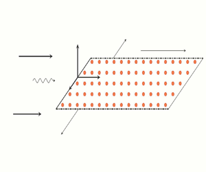
This solution depends heavily on the boundary conditions prescribed on the plate. Before discussing these conditions, we will briefly outline the governing equations for the gust-scattering solution. Figure 2 demonstrates how we mathematically model the leading-edge noise problem. We assume that the plate is semi-infinite in the streamwise direction  $x$, and infinite in the spanwise direction $z$, and is situated at the wall-normal position $y=0$. We will assume that the plate has zero thickness and that all quantities are time-harmonic with assumed $\exp ({-\textrm {i}\omega t})$ dependence, which subsequently will be suppressed. For simplicity, we solve for the scattered acoustic potential $\phi _s$, which relates to the scattered pressure $p_s$ via the non-dimensionalised relation
 \begin{equation} p_s={-}\rho_0\left(U_c\,\frac{\partial}{\partial x}-{\rm i}\omega\right)\phi_s, \end{equation}
with  $\rho _0$ the ambient fluid density, and $U_c$ the mean flow convection velocity at the leading edge. Our model accounts for constant mean flow that convects at some velocity $U_c\neq U_{\infty }$. For some applications, when no change is expected in this velocity, it suffices to set $U_c=U_{\infty }$. Our scattered pressure solution solves the convected Helmholtz equation
 \begin{equation} (1-M_c^2)\,\frac{\partial^2 \phi_s}{\partial x^2} +\frac{\partial^2 \phi_s}{\partial y^2} +2{\rm i}k_1M_c^2\, \frac{\partial \phi_s}{\partial x} +(M_c^2k_1^2-k_3^2)\phi_s=0,\end{equation}
where  $M_c=U_c/c_0$ is the Mach number for the convective mean flow. We apply Taylor's frozen turbulence hypothesis, and assume $k=M_ck_1$. Physically speaking, individual turbulent eddies convect with the mean flow. We also assume that the scattered potential is continuous across $x<0$, i.e. $\phi _s(x,0^+)-\phi _s(x,0^-)=0$, and on the plate, we use an impedance boundary condition for the total field
 \begin{equation} p=\rho_0c_0Z\,\frac{\partial \phi}{\partial n}, \end{equation}
where we define  $Z$ as the non-dimensional specific impedance, and assume that our normal vector points out of the fluid and into the boundary (for consistency with Rawlins Reference Rawlins1975; Rienstra & Hirschberg Reference Rienstra and Hirschberg1992; Barton & Rawlins Reference Barton and Rawlins1999).
Mathematical set-up for an incident gust scattering off a semi-infinite porous plate.

Next, we introduce the important convective constant  $\beta =\sqrt {1-M_c^2}$ and then ensure that our governing equation is a Helmholtz equation by introducing a convective transform
 \begin{equation} \widetilde{\phi_s}(x,y)= \phi_s(x,y)\exp\left({\frac{{\rm i}k_1M_c^2x}{\beta^2}}\right), \end{equation}
followed by the Prandtl–Glauert transformation
 \begin{equation} \tilde{\tilde{\phi}}_s(x,y)=\tilde{\phi}_s(\beta x,y). \end{equation}
Each transform must also be applied to our boundary conditions. With this, after dropping tildes, we obtain the following governing equations:
 $$\begin{gather} \frac{\partial^2\phi_s}{\partial x^2}+\frac{\partial^2\phi_s}{\partial y^2}+{k^*}^2\phi_s=0, \end{gather}$$
 $$\begin{gather}\mp\frac{\partial \phi_s}{\partial y}+\frac{M_c}{\beta Z}\,\frac{\partial \phi_s}{\partial x}-\frac{{\rm i}k^*}{\beta^2 Z}\,\phi_s={\pm} {\rm i} k_2\,{\rm e}^{{\rm i}\tilde{k}x},\quad x>0,\enspace y=0^\pm, \end{gather}$$
 $$\begin{gather}\phi_s(x,0^+)-\phi_s(x,0^-)=0,\quad x<0, \end{gather}$$
 $$\begin{gather}\frac{\partial \phi_s}{\partial y}(x,0^+)-\frac{\partial \phi_s}{\partial y}=0,\quad x<0. \end{gather}$$
These equations contain two important wavenumbers,
 \begin{equation} k^*=\frac{\sqrt{M_c^2k_1^2-\beta^2k_3^2}}{\beta},\quad \tilde{k}=\frac{k_1}{\beta^3}, \end{equation}
i.e. the convective Helmholtz wavenumber and the source wavenumber, respectively.
To construct an analytical solution, we use the Wiener–Hopf technique. In particular, we follow the method of Barton & Rawlins (Reference Barton and Rawlins1999, Reference Barton and Rawlins2005), Rawlins (Reference Rawlins1975) and Hales & Ayton (Reference Hales and Ayton2024). This method begins by taking a solution of the form
 \begin{equation} \phi_s(x,y)=\frac{1}{2{\rm \pi}}\int_{-\infty}^{\infty}\begin{pmatrix} A(\alpha)\\ B(\alpha) \end{pmatrix}\exp({-{\rm i}\alpha x-\gamma\,|y|})\,\textrm{d}\alpha, \end{equation}
where  $\gamma =\sqrt {\alpha ^2-{k^*}^2}$ is a complex function of $\alpha$ whose branch cuts $\varGamma ^{\pm }$ emanating from ${\pm }k$ are chosen to extend to ${\pm }\infty$ as in figure 3. We choose these branch cuts to ensure that integration along the real line avoids the branch points. Moreover, our chosen branch cuts will ensure $\textrm {Re}[\gamma ]>0$ when $\alpha$ is in the region of overlap defined in the Wiener–Hopf technique, or when $|\textrm {Re}[\alpha ]|>|\textrm {Re}[k^*]|$. Since our wavenumbers will always be real (or have negligibly small imaginary parts for analytic purposes) for our application, this is favourable compared to horizontal branch cuts extending from ${\pm }k^*$ to $\pm \infty$, respectively.
Demonstration of branch cuts  $\varGamma ^{k,-k}$ and the values that $\gamma (\alpha )$ takes on each side. We take the square root in the diagram as the principal square root.

To obtain a Wiener–Hopf equation, we Fourier transform our solution (3.8) along the real line and implement all our boundary conditions. For example, Fourier transforming our boundary condition on the upper side plate gives
 \begin{align} & \left(\gamma-\frac{{\rm i}M_c}{\beta Z}\,\alpha-\frac{{\rm i}k^*}{\beta^2 Z}\right)A(\alpha) \nonumber\\ &\quad =\int_{-\infty}^{0}\left(-\frac{\partial \phi_s}{\partial y}+\frac{M_c}{\beta Z} \frac{\partial \phi_s}{\partial x}-\frac{{\rm i}k^*}{\beta^2 Z} \phi_s\right){\rm e}^{{\rm i}\alpha x}\,\textrm{d}\kern0.06em x \nonumber\\ &\qquad +\int_{0}^\infty \left(-\frac{\partial \phi_s}{\partial y}+\frac{M_c}{\beta Z}\, \frac{\partial \phi_s}{\partial x}-\frac{{\rm i}k^*}{\beta^2 Z}\,\phi_s\right) {\rm e}^{{\rm i}\alpha x}\,\textrm{d}\kern0.06em x \nonumber\\ &\quad =\int_{-\infty}^{0}\left(-\frac{\partial \phi_s}{\partial y}+\frac{M_c}{\beta Z}\, \frac{\partial \phi_s}{\partial x}-\frac{{\rm i}k^*}{\beta^2 Z}\, \phi_s\right){\rm e}^{{\rm i}\alpha x}\,\textrm{d}\kern0.06em x-\frac{k_2}{\alpha+\tilde{k}} \nonumber\\ &\quad :=L_1 -\frac{k_2}{\alpha+\tilde{k}}. \end{align}
 We use the notation  $L_1$ to denote that this integral term is an unknown in our system that is analytic in the lower half-plane. Therefore, if we define our lower region for the Wiener–Hopf technique to be $\textrm {Im}[\alpha ]<\textrm {Im}[k^*]$, and write this as $D_L$, then we see that $L_{1}$ can be defined as a lower analytic function. Similarly, the second term will be analytic in the region $\textrm {Im}[\alpha ]>-\tilde {k}$. We will define this as our upper region, and write this as $D_U$, so that this function is an upper analytic function. It can be seen that $D_L\cap D_U\neq \emptyset$ and $D_L\cup D_U=\mathbb {C}$.
Omitting the details, we repeat this procedure for the other three boundary conditions in (3.6) and obtain the matrix system
 \begin{equation} \kappa\begin{pmatrix} 1 & -{1}/{\gamma}\\ -1 & -{1}/{\gamma} \end{pmatrix}\begin{pmatrix} u\\ v \end{pmatrix}=2\begin{pmatrix} L_1 \\ L_2 \end{pmatrix}+ \frac{2k_2}{\alpha+\tilde{k}} \begin{pmatrix} 1\\ -1 \end{pmatrix}. \end{equation}
This can be defined in shorthand notation as
 \begin{equation} \kappa\,\boldsymbol{\mathsf{K}}\, \boldsymbol{U}=\boldsymbol{L}+\boldsymbol{S}, \end{equation}
which has two upper analytic unknowns  $U_{1,2}$, and two lower analytic unknowns $L_{1,2}$, alongside an upper analytic source term $\boldsymbol{S}$. An important component of our Wiener–Hopf equation is the scalar kernel $\kappa$ that we define as
 \begin{equation} \kappa(\alpha)=\gamma-\frac{{\rm i}M_c\beta}{Z}\,\alpha-\frac{{\rm i}k^*}{\beta^2 Z}. \end{equation}
This is consistent with the kernel in both Rawlins (Reference Rawlins1975) and Barton & Rawlins (Reference Barton and Rawlins1999). To solve this system, we rearrange to ensure the left-hand side of the equation is analytic in the lower region  $D_L$, and the right-hand side is analytic in $D_U$. Then we deduce that each side is equal to some entire function $\boldsymbol{E}$ that is analytic in $\mathbb {C}$.
For this, we define the additive factorisation of any tensor  $f$ as a splitting
 \begin{equation} f=(f)_+ + (f)_-, \end{equation}
with  $f_{\pm }$ analytic in $D_U$ ( $D_L$). We define the multiplicative factorisation of any tensor $f$ as a splitting
 \begin{equation} f=f^+f^-, \end{equation}
with  $f_{\pm }$ analytic in $D_U$ ( $D_L$).
Using this notation, we re-write our Wiener–Hopf equation (3.11) as
 \begin{equation} \underbrace{\kappa^+\boldsymbol{\mathsf{K}}^+\boldsymbol{U} -\left(\frac{2}{\kappa^-}\,(\boldsymbol{\mathsf{K}}^-)^{{-}1} \boldsymbol{S}\right)_+}_{{upper\ analytic}}=\underbrace{\frac{2}{\kappa^-}\, (\boldsymbol{\mathsf{K}}^-)^{{-}1}\boldsymbol{L}+\left(\frac{2}{\kappa^-} (\boldsymbol{\mathsf{K}}^-)^{{-}1}\boldsymbol{S}\right)_- }_{{lower\ analytic}}= \underbrace{\boldsymbol{E}}_{{entire}}.\end{equation}
We address each set of factors in turn.
3.1. Additive factorisations
We split the tensor
 \begin{equation} \frac{2}{\kappa^-(\alpha)}\,(\boldsymbol{\mathsf{K}}^-)^{{-}1}(\alpha)\, \boldsymbol{S}(\alpha) \end{equation}
using the method of pole removal. Since  $\boldsymbol{S}(\alpha )$ is analytic in $\mathbb {C}\setminus \{-\tilde {k}\}$, the factorisation will be
 \begin{equation} \left.\begin{gathered} ((\boldsymbol{\mathsf{K}}^-)^{{-}1}\boldsymbol{S})_+ = \frac{2}{\kappa^-(-\tilde{k})}\,(\boldsymbol{\mathsf{K}}^-)^{{-}1} (-\tilde{k})\, \boldsymbol{S}(\alpha),\\ ((\boldsymbol{\mathsf{K}}^-)^{{-}1}\boldsymbol{S})_-{=} \left(\frac{2}{\kappa^-(\alpha)}\,(\boldsymbol{\mathsf{K}}^-)^{{-}1} (\alpha)\, \boldsymbol{S}(\alpha)-\frac{2}{\kappa^-(-\tilde{k})}\, (\boldsymbol{\mathsf{K}}^-)^{{-}1} (-\tilde{k})\, \boldsymbol{S}(\alpha)\right). \end{gathered}\right\} \end{equation}
3.2. Multiplicative factorisations
The two important terms to split multiplicatively are the matrix kernel  $\boldsymbol{\mathsf{K}}$ (note that our matrix Wiener–Hopf equation dictates that our splitting must be $\boldsymbol{\mathsf{K}} =\boldsymbol{\mathsf{K}}^- \boldsymbol{\mathsf{K}}^+$, and this factorisation is not commutative, unlike the scalar case) and the scalar kernel $\kappa$. The former can be split by inspection:
 \begin{equation}
\boldsymbol{\mathsf{K}}=\begin{pmatrix} 1 &
-\dfrac{1}{\gamma^-(\alpha)}\\ -1 &
-\dfrac{1}{\gamma^-(\alpha)} \end{pmatrix} \begin{pmatrix}
1 & 0\\ 0 & \dfrac{1}{\gamma^+(\alpha)}
\end{pmatrix},\end{equation}
\begin{equation}
\boldsymbol{\mathsf{K}}=\begin{pmatrix} 1 &
-\dfrac{1}{\gamma^-(\alpha)}\\ -1 &
-\dfrac{1}{\gamma^-(\alpha)} \end{pmatrix} \begin{pmatrix}
1 & 0\\ 0 & \dfrac{1}{\gamma^+(\alpha)}
\end{pmatrix},\end{equation}
where  $\gamma ^\pm (\alpha )$ denotes the multiplicative factorisation of $\gamma$,
 \begin{equation} \gamma^+(\alpha)=\sqrt{-{\rm i}(\alpha+k^*)},\quad \gamma^-(\alpha)=\sqrt{{\rm i}(\alpha-k^*)}. \end{equation}
However,  $\kappa (\alpha )$ is split with more care in Appendix A. It is reliant on the Maliuzhinets function for quarter-plane problems,
 \begin{equation} \psi_{{\rm \pi}/{2}}(z)=\exp\left(\int_{0}^z\frac{2\zeta-{\rm \pi}\sin(\zeta)}{\cos(\zeta)}\,\textrm{d}\zeta\right), \end{equation}
which can be evaluated efficiently using numerical collocation methods from Aidi & Lavergnat (Reference Aidi and Lavergnat1996). Introducing  $\mathfrak {E}(s)$ to be a holomorphic eigensolution to the governing difference equation, we derive the solution for $\kappa ^+$ in the hyperbolic geometry defined by $\alpha =-k^*\sin s$:
 \begin{equation} \left.\begin{gathered} \kappa^+(k^*\sin(s))\\ =\mathfrak{E}(s)\,\sqrt{-{\rm i}k^*} \sqrt{\frac{\cos(\delta)+\sin(X)}{\cos(\delta)}}\, \frac{\psi_{{\rm \pi}/{2}}(s-X-\delta+{\rm \pi})\,\psi_{{\rm \pi}/{2}}(s+X-\delta)}{\psi_{{\rm \pi}/{2}}(X+\delta)\, \psi_{{\rm \pi}/{2}}(X-\delta-{\rm \pi})},\\ \delta =\arctan\left(-\frac{M\beta}{Z}\right),\quad X={-}\arcsin\left(-\frac{1}{\beta^2\sqrt{Z^2+M^2\beta^2}}\right)-{\rm \pi}. \end{gathered}\right\} \end{equation}
The latter equation that defines  $X$ will ensure that it lies in the region
 \begin{equation} \left.\begin{gathered} {\rm Re}[X] \in\left(-{\rm \pi},\frac{\rm \pi}{2}\right],\quad {\rm Im}[X]\in [0,\infty),\\ {\rm Re}[X] \in\left[0,\frac{\rm \pi}{2}\right),\quad {\rm Im}[X]\in [-\infty,0), \end{gathered}\right\} \end{equation}
as chosen in Abrahams & Lawrie (Reference Abrahams and Lawrie1995). We can compute  $\kappa ^-$ via $\kappa ^-={\kappa }/{\kappa ^+}$.
For this derivation, we have implemented the hyperbolic transformation  $\alpha =-k^*\sin (s),$ from Abrahams & Lawrie (Reference Abrahams and Lawrie1995), and choose $\mathfrak {E}$ to be an eigensolution (suitable holomorphic function) that ensures that each factor is analytic in the required half-plane. For almost all sensible values of $Z$,
$Z$,  $\mathfrak {E}=1$. However, if $\kappa$ has a zero in the cut $\alpha$-plane, such as in the upper half-plane, then we amend the factorisation to ensure that the zero of $\kappa$ features in the factor $\kappa ^-$. This process is touched upon in Abrahams & Lawrie (Reference Abrahams and Lawrie1995) in terms of eigensolutions to the hyperbolic difference equation solved by the kernel. At the same time, it is hinted at in Barton & Rawlins (Reference Barton and Rawlins1999), Rawlins (Reference Rawlins1975) and Ahmad (Reference Ahmad2006) as requiring residues to be calculated during the Cauchy integral formulation of the factorisation. More details are omitted in Appendix A.
In Appendix B, we show that the entire function satisfies  $\boldsymbol{E}=0$, so we can solve for $\boldsymbol{L}$:
 \begin{equation} \boldsymbol{L}=\boldsymbol{\mathsf{I}}\, \boldsymbol{S}(\alpha)- \frac{\kappa^-(\alpha)}{\kappa^-(-\tilde{k})}\,\boldsymbol{\mathsf{K}}^-(\alpha)\, (\boldsymbol{\mathsf{K}}^-)^{{-}1}(-\tilde{k})\, \boldsymbol{S}(\alpha),\end{equation}
and deduce
 \begin{equation} \begin{pmatrix} A(\alpha) \\ B(\alpha) \end{pmatrix}=\frac{k_2}{\alpha+\tilde{k}}\, \frac{1}{\kappa^+(\alpha)\,\kappa^-(-\tilde{k})} \begin{pmatrix} 1 \\ -1 \end{pmatrix}.\end{equation}
As one may expect, the solution is an odd function of  $y$. However, this may not always be the case, so we retain the matrix structuring of our argument to ensure its applicability to future examples involving more complicated boundary conditions and source terms.
Now that we have found  $\phi _s$, we undo the convective coordinate changes, albeit leaving our solution in Prandtl–Glauert space (our study uses Mach numbers between 0.1 and 0.2, for which the effects of the Prandtl–Glauert transform have been noted to have little effect; see Hales et al. Reference Hales, Ayton, Jiang, Mahgoub, Kisler, Dixon, de Silva, Moreau and Doolan2023), so that
 \begin{equation} p_s(x,y)=\frac{{\rm i}\exp\left(\dfrac{-{\rm i}k_1M^2x}{\beta^2}\right)}{{2{\rm \pi}}\beta^2}\int_{-\infty}^{\infty} \begin{pmatrix} A(\alpha) \\ B(\alpha) \end{pmatrix}\left(\frac{\alpha}{\beta}+\frac{k_1}{\beta^2}\right) \exp\left({-{\rm i}\,\frac{\alpha}{ \beta}\,x-\gamma\,|y|}\right)\textrm{d}\alpha, \end{equation}
which has been non-dimensionalised. Then we can obtain our transfer function  ${g}$ by calculating the far-field pressure solution defined as
 \begin{equation} P_{gust}(\boldsymbol{k},\theta)=\lim_{r\to\infty}\sqrt{r}\,p_s(r,\theta)\end{equation}
via the method of steepest descent,
 \begin{equation} P_{gust}(\boldsymbol{k},\theta)\sim \exp({{\rm i}k^*r})\, \sqrt{\frac{k^*}{2{\rm \pi} {\rm i}}}\,\frac{\sin(\theta)}{\beta^3}\, ({k_1}-k^*\cos(\theta)\,\beta^2)A({-}k^*\cos(\theta)),\end{equation}
from which
 \begin{equation} g(\boldsymbol{k},\theta)\sim\frac{k^*\sin^2(\theta)}{2{\rm \pi} \beta^4}\, |(k_1-k^*\cos(\theta)\,\beta^3)A({-}k^*\cos(\theta))|^2.\end{equation}
Similar results follow for  $-{\rm \pi} <\theta <0$ but are not necessary for implementation within this particular experimental study since our observer angle is fixed at $\theta ={{\rm \pi} }/{2}$.
4. Experimental methods
As mentioned previously, the experimental aspects of this paper can be considered a unification and evolution of the work done in Hales et al. (Reference Hales, Ayton, Jiang, Mahgoub, Kisler, Dixon, de Silva, Moreau and Doolan2023) (for the turbulence aspects) and Ayton et al. (Reference Ayton, Karapiperis, Awasthi, Moreau and Doolan2021b) (for the porosity aspects). Specific details can be found in each of these papers; nonetheless, we will highlight the essential features of the experiment in this section.
The noise measurements were performed at the University of New South Wales (UNSW) in the open jet anechoic wind tunnel, which has test section area  $0.455\,\textrm {m}\times 0.455\,\textrm {m}$ and chamber size $3\,\textrm {m}\times 4.17\,\textrm {m}\times 2.15\,\textrm {m}$. The free-stream turbulence intensity is 0.7 % at $20\,\textrm {m s}^{-1}$. Figure 4 shows a schematic of the tunnel. Further details about the tunnel can be found in Moreau et al. (Reference Moreau, de Silva, Kisler, Tan, Jiang, Awasthi and Doolan2022). Leading-edge inserts with thickness $T=1.5\,\textrm {mm}$ are fixed onto a flat plate aerofoil as described by schematics in figure 5; three porous inserts studied in Ayton et al. (Reference Ayton, Karapiperis, Awasthi, Moreau and Doolan2021b) were used as well as the standard rigid leading-edge insert used in Hales et al. (Reference Hales, Ayton, Jiang, Mahgoub, Kisler, Dixon, de Silva, Moreau and Doolan2023).
Schematic of UNSW anechoic wind tunnel.

Schematics of the flat plate aerofoil test model (where LE means leading edge, and TE means trailing edge). Figure adapted and used with the authors’ permission from Ayton et al. (Reference Ayton, Karapiperis, Awasthi, Moreau and Doolan2021b).

4.1. Test cases and model parameters
4.1.1. Flow parameters
The flow conditions used for this experiment are an exact subset of those explored in Hales et al. (Reference Hales, Ayton, Kisler, Mahgoub, Jiang, Dixon, de Silva, Moreau and Doolan2022, Reference Hales, Ayton, Jiang, Mahgoub, Kisler, Dixon, de Silva, Moreau and Doolan2023). This previous experimental campaign used PIV to characterise the properties of the flow.
A cylinder of diameter  $D=22$ mm was placed $6D$ upstream of the measurement field of view (FOV) to generate anisotropic turbulence in its wake region. The measurement FOV for the PIV measurement is on an $(x,y)$-plane and has dimensions $286\,\textrm {mm}\times 143\,\textrm {mm}$ in the streamwise ( $x$) and vertical ( $y$) directions, respectively. The origin of the coordinate system is located at the centre of the cylinder. The measurement FOV covers a streamwise distance between $\Delta x = 6D$ and $\Delta x = 19D$, and a vertical distance between $\Delta y = - 3.25D$ and $\Delta y = 3.25D$. The PIV uncertainty is approximately 0.1 pixels (Adrian & Westerweel Reference Adrian and Westerweel2011), corresponding to $\pm$5 microns in the present work. The results were calculated using $32\times 32$ pixels interrogation windows. The error in the calculated velocity is $\pm$0.3125. For a representative example, the uncertainty for the convection velocity $U_c$ at $x/D = 9.5$ is $0.046\,\textrm {m s}^{-1}$, which can be considered negligible.
Details of this process can be found in Hales et al. (Reference Hales, Ayton, Jiang, Mahgoub, Kisler, Dixon, de Silva, Moreau and Doolan2023). Experiments were conducted at mean flow velocities  $U_{\infty }=20, 28\,\textrm {m s}^{-1}$. The flat plate aerofoil was placed in the centre of the cylinder wake at locations $x/D = 9.5, 12.5$ downstream from the cylinder, where $x = 0$ refers to the centre of the cylinder. The required data for the model from each of these configurations are listed in table 2. We list all values in one table for simplicity; note that the convection velocity $U_c$ is not equal to the free-stream velocity as this is measured close to the leading edge. As discussed in Hales et al. (Reference Hales, Ayton, Jiang, Mahgoub, Kisler, Dixon, de Silva, Moreau and Doolan2023), this convection velocity is slower than the free-stream velocity due to the interaction with the cylinder.
Turbulent flow model parameters.

To demonstrate how flow anisotropy varies with the streamwise direction  $x$, we plot the ratios $\varLambda _r$ and $u_r$ against the distance $x/D$ in figure 6.
Variation of length scale and root-mean-square velocity ratios with distance  $x/D$ from the cylinder: (a) variation in $\varLambda _2/\varLambda _1$; (b) variation in $v/u$.

4.1.2. Porosity parameters
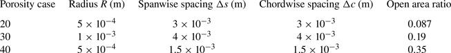
Despite the larger scope of the experiments performed on porous inserts with spanwise variability in Ayton et al. (Reference Ayton, Karapiperis, Awasthi, Moreau and Doolan2021b), for this preliminary testing of our model, we focused only on non-varying porous cases. We present representative porosity samples in figure 7 and outline the key parameter values that distinguish them in table 3. We will use impedance models for porous plates that are based on the Leppington model
 \begin{equation} Z_1(\omega)=\frac{-{\rm i}\omega {\rm \pi}R}{4c_0 \alpha_H},\end{equation}
which depends directly on the pore radius ( $R$) and the open area ratio ( $\alpha _H$), defined as
 \begin{equation} \alpha_H=\frac{R^2{\rm \pi}}{\Delta s\,\Delta c} \end{equation}
where we have defined  $\Delta s$ as the spanwise spacing between pores from centre to centre, and $\Delta c$ as the chordwise spacing between pores from centre to centre. For each porosity case tested, $\Delta s = \Delta c$.
The 3-D printed samples of the three porosities investigated in this experiment: left, case 30; middle, case 20; right, case 40. Case 40 has the finest porous structure, but has the smallest distance between pores. Thus it has the largest open area ratio due to the large number of pores per unit area.

Porosity model parameters.
A correct mathematical model for the impedance of a perforated sheet is an open problem that has led to many models of varying intricacy. These models also vary in the flow profiles and porosities to which they are applicable. A curve-fitting approach is taken in Chen, Ji & Huang (Reference Chen, Ji and Huang2020), resulting in a model that fits several datasets, as seen in figures 13 and 14 of this paper. These figures also compare several other models, including the Howe model that is similar to (4.1). However, this approach demonstrates no universal agreement on how to model impedance in flow; curve fitting based on physical observations and an analytical model appears to be the best approach.
In the next subsection, we will return to the impedance modelling, where we will design an impedance function based on empirical models that give the best agreement for the leading-edge noise model.
4.2. Noise measurements
The acoustic measurements are undertaken with a phased microphone array with 64 microphones arranged in a spiral shape to optimise beamforming localisation and quantification accuracy. Figure 8 shows a schematic of the noise measurement experiment. The microphone array is positioned in the aerofoil's far field with its surface plane parallel to its symmetry plane and its centre microphone aligned with its leading-edge centre. The 64 microphones simultaneously record time signals with sampling rate 65 536 Hz. For the determination of the frequency spectra of the radiated leading-edge noise, the narrowband beamforming results have been obtained using the source power integration method, which normalises out the effect of the point spread function on the phased microphone array output (Brooks & Humphreys Reference Brooks and Humphreys1999).
Schematic for the acoustics measurements of leading-edge noise in anisotropic turbulence. The leading-edge insert can be replaced with porous inserts as shown in figure 3 of Ayton et al. (Reference Ayton, Karapiperis, Awasthi, Moreau and Doolan2021b).

We display comparative beamforming maps for two porous leading-edge cases, 20 and 30. The beamforming results were processed using ‘diagonal removal’, where we set the autospectral elements of the cross-spectral matrix (CSM) to 0, improving the array's signal-to-noise ratio (SNR). The array design and deconvolution of the beamformer output minimise spatial aliasing effects.
Background noise removal was also included, where the CSM of the background case (cylinder in, flow on, no aerofoil) was subtracted from the CSM of the test case with the aerofoil. This reduces the influence of the cylinder or the tunnel inlet on beamforming results. The beamforming maps in figure 9 are in dB, with the dynamic range of the plots set to 10 dB. The turbulent inflow produces a strong noise source at the leading edge. The region at the trailing edge is kept comparatively quiet due to the trailing-edge serrations. At higher frequencies (6 kHz), the SNR is noticeably lower. The black lines in all these plots show the aerofoil's location, the leading-edge insert's chordwise extent, and the upper and lower wall plates. Figure 10 reproduces beamforming maps for the porous case 40 at the same frequencies, mean flow velocity and cylinder position. We observe that the source shapes are nearly identical, but the levels are lower.
Beamforming maps for the case 20 porous insert at three frequencies and mean flow velocity  $28\,\textrm {m s}^{-1}$. The cylinder is $12.5D$ upstream of the leading edge. The flow is from left to right, and the colour bar scale is given in dB.

Beamforming maps for the case 40 porous insert at three frequencies and mean flow velocity  $28\,\textrm {m s}^{-1}$. The cylinder is $12.5D$ upstream of the leading edge. The flow is from left to right, and the colour bar scale is given in dB.

The narrowband beamforming output maps are integrated over a region located at the central part of the leading edge to obtain the frequency spectrum of the sound pressure level (SPL) generated by the free-stream turbulence interacting solely with the leading edge. The integration area is centred on the mid-span, measures 0.2 m streamwise and 0.3 m spanwise, and was kept consistent for all cases, as shown in figure 11. This ensures that noise generated by the interaction of the wind tunnel wall boundary layers with the aerofoil junction are rejected from the pressure spectrum. This is demonstrated for the porous case 20 at 4000 Hz in figure 11. The noise spectra are presented as a PSD in  $\textrm {dB Hz}^{-1}$
Region of integration for beamforming to obtain the frequency spectrum of the leading-edge SPL. The flow is from left to right, and the colour bar scale is given in dB.

5. Model validation and experimental findings
To approximate the leading-edge noise with our mathematical model, we use a non-dimensionalised model by considering a turbulence spectrum and gust solution independent of the length scales of the model. First, we define a dimensional length scale  $L$ to be the plate's total chord length (0.352 m). Second, we define a dimensional velocity $U$ to be the convection velocity $U_c$. This convection velocity is calculated as the edge velocity $U_e$, the mean flow velocity measured in the vicinity of the plate. For simplicity, we will always refer to this quantity as $U_c$. To ensure that our approximated SPL has the correct dimensions, we will multiply by $U/\sqrt {L}$. Finally, we divide the result by a reference pressure $p_a=2\times 10^{-5}\,\textrm {Pa}$, then calibrate with a vertical shift by a constant $C=29$, which effectively aligns our reference pressure to match experimentally. Thus the SPL $\mathcal {P}$ is written in terms of $\varPsi$ via
 \begin{equation} \mathcal{P}(\,{f})=20 \log_{10} \left(\frac{U\,\varPsi(f,{\rm \pi}/2)}{\sqrt{L}\,p_a}\right) + 29. \end{equation}
The calibration constant is much lower than the rigid plate model in Hales et al. (Reference Hales, Ayton, Jiang, Mahgoub, Kisler, Dixon, de Silva, Moreau and Doolan2023) since that solution scaled like  $M^2$ due to different changes in variables. This model also corrects the multiplying dimensionalisation constants from the previous model.
5.1. Experimental results
Before testing our model, we discuss the results of our experiment. First, we investigate the effects of velocity and distance from the cylinder ( $x/D$) on measured leading-edge noise for both the rigid plate and the three tested porous cases. As expected, figure 12 shows that a higher flow velocity results in a broadband increase in noise generation at the leading edge for all tested leading-edge inserts. In addition, as we found in Hales et al. (Reference Hales, Ayton, Jiang, Mahgoub, Kisler, Dixon, de Silva, Moreau and Doolan2023), increasing the cylinder distance from $9.5$ to $12.5$ decreases the noise by approximately 1–2 dB. This is hypothesised to be due primarily to the smaller $u_r$ ratio when comparing $x/D=12.5$ to $x/D=9.5$. One observation for every flow condition is an unexpected increase of approximately 1–4 dB between 4 and 6 kHz. We believe that this is due to scrubbing noise from the grazing flow as it passes over the porous surfaces. Roughness noise is a key contributor to high-frequency noise for porous leading edges, as discussed in Jiang et al. (Reference Jiang, Moreau, de Silva and Doolan2024). However, it is not incorporated within our leading-edge model, and is removed from the rest of this study. We will exclude the extremes of our frequency range for model comparisons and focus on the low- and mid-frequency ranges where the impedance-based model best describes the expected noise reduction due to porosity. Next, in figure 13, we examine the changes in SPL for each porous test case at each flow condition.
Comparisons for all tested leading-edge inserts as flow conditions (inflow velocity and cylinder distance) are changed: (a) rigid insert; (b) case 20 insert; (c) case 30 insert; (d) case 40 insert.

Noise reduction ( $\Delta$SPL) for each flow condition when comparing the SPL from the rigid insert to each of the three porous insert cases tested: (a) $U_{\infty }=20\,\textrm {m s}^{-1}$, $x/D=9.5$; (b) $U_{\infty }=20\,\textrm {m s}^{-1}$, $x/D=12.5$; (c) $U_{\infty }=28\,\textrm {m s}^{-1}$, $x/D=9.5$; (d) $U_{\infty }=28\,\textrm {m s}^{-1}$, $x/D=12.5$.

5.2. Calibrating the rigid model
Before we investigate porosity within our theoretical model, we calibrate the rigid model to the experimental data.
Previous experimental measurements of flow statistics for turbulence past a cylinder suggested  $u\approx 1.2w$. We take this as an estimated starting point to implement the 3-D turbulence spectrum within our model against our current experimental data. It is unclear what to expect from the integral length $\varLambda _3$; we test several options for this.
First, we set  $u=1.2w$ and $\varLambda _1=1.2\varLambda _3$. Second, we set $u=1.2w$ and choose $\varLambda _3=\varLambda _1$. In addition to these, we present a tailored case for each flow condition in which we choose $w$ and $\varLambda _3$ to fit the data best. We chose these tailored values based on observations from the first couple of trialled ratios. First, it seemed preferable to keep $\varLambda _3\leq \varLambda _1$ since this shifted the spectrum's peak to the left, showing better agreement at the low-frequency range. However, having ${u}/{w}\geq 1.2$ was also important to compensate for this shift and to see a better agreement for the whole frequency range.
All values required for the 3-D model are listed in table 4.
For the rigid case, these examples are compared with the original axisymmetric assumption in figure 14 for all flow conditions. Our new model compensates for the necessary shift to the left (previously dealt with using a scaling factor) with values of  $w$ smaller than those used for the axisymmetric assumption. We see far better agreement across almost all frequencies when using the new turbulence model. We feel that this is a better way to model the problem than the previous artificial $\varrho$ shift since it is based on expected observations in an empirical manner.
Comparison of predicted leading-edge noise when varying streamwise to spanwise ratios within the turbulence model. Each flow condition is tested, and only the rigid model is used: (a)  $U_{\infty }=20\,\textrm {m s}^{-1}$, $x/D=9.5$; (b) $U_{\infty }=20\,\textrm {m s}^{-1}$, $x/D=12.5$; (c) $U_{\infty }=28\,\textrm {m s}^{-1}$, $x/D=9.5$; (d) $U_{\infty }=28\,\textrm {m s}^{-1}$, $x/D=12.5$.

Suggested tailored  $w$ and $\varLambda _3$ values for each flow condition.

5.3. Predictions and validation for a perforated leading edge
5.3.1. Comparing homogenised impedance models for perforated plates
First, we will discuss how we model our specific impedance  $Z(\omega )$. As mentioned in Naqvi & Ayton (Reference Naqvi and Ayton2022), this is an open area of research, and there is no universal agreement on what model is best. For our study, we initially tested four models for the first flow condition $U_{\infty }=20\,\textrm {m s}^{-1}$, $x/D=9.5$ and for the case 20 porous insert. The first model is Leppington's model derived in Leppington (Reference Leppington1977) for a porous plate, defined in (4.1) as $Z_1(\omega )$.
The primary drawback of this model is that it does not account for grazing flow. We refer to work completed in Howe et al. (Reference Howe, Scott and Sipcic1996) to incorporate flow within the impedance. In this paper, the Rayleigh conductivity  $K_R$ is altered to account for the effects of grazing flow. The simplest definition for Rayleigh conductivity is that it measures the ease with which sound waves can pass through circular orifices. Howe's model for the impedance of a circular orifice is
 \begin{equation} Z_H(\omega)={-}\frac{{\rm i}k_0{\rm \pi} R^2}{2K_R}. \end{equation}
Without flow, the Rayleigh conductivity is equal to  $2R$. With flow, it becomes
 \begin{equation} \left.\begin{gathered} K_R^f=2R(\varGamma-{\rm i}\delta),\\ \varGamma-{\rm i}\delta=1+\frac{({\rm \pi}/2)\,{\rm I}_1(Sr) \,{\rm e}^{-{Sr}}-{\rm i}\,{\rm K}_1({Sr})\sinh({Sr})}{{Sr} \left(({\rm \pi}/2)\,{\rm I}_1({Sr})\,{\rm e}^{-{Sr}}+{\rm i}\,{\rm K}_1({Sr})\cosh({Sr})\right)},\quad {Sr}=\frac{\omega R}{U_c}, \end{gathered}\right\} \end{equation}
where  ${Sr}$ is the (convective) Strouhal number, and $\mathrm {I}_1, \mathrm {K}_1$ are modified Bessel functions of the first and second kind. If we rewrite the impedance model (4.1) as
 \begin{equation} Z_1(\omega)={-}\frac{{\rm i}k_0{\rm \pi} R^2}{\alpha_HK_R}, \end{equation}
then we can implement Howe's Rayleigh conductivity for a circular aperture in grazing flow (Howe Reference Howe1998) within the no-flow impedance model (4.1):
 \begin{equation} Z_2(\omega)=\frac{Z_1(\omega)}{\varGamma-{\rm i}\delta}. \end{equation}
Our first acoustic comparisons will compare the Leppington and Howe models with or without flow. We remain with the case 20 porosity and flow conditions from  $U_{\infty }=20\,\textrm {m s}^{-1}$, $x/D=9.5$. From figure 15, the best model is the Leppington model with flow effects, although there is still an overprediction of noise at all frequencies (especially the high-frequency regime). The Howe model works better without flow. In fact, including flow appears to have a detrimental effect. We will choose the best-performing model $Z_2$, but seek further physically inspired analytical amendments to improve the agreement across all frequencies.
Model comparisons using the Leppington (4.1) and Howe (5.2) impedance models with or without amendments for flow. The four tested impedance models are the Leppington model ( $Z_1$) from (4.1), the Leppington model accounting for flow ( $Z_2$) from (5.5), the Howe model ( $Z_H$) from (5.2) and finally the Howe model that accounts for flow.

One amendment that we may make to this model is to account for plate thickness  $T$. This parameter may be important for some experimental cases (Jing et al. Reference Jing, Sun, Wu and Meng2012). In Luong et al. (Reference Luong, Howe and McGowan2005), a new simplified model for the Rayleigh conductivity based on the Cummings equation that included a simpler asymptotic approximation to $\varGamma -\textrm {i}\delta$ was constructed that accounted for thickness:
 \begin{equation} \left.\begin{gathered} K_R^T=K_0(\tilde{\varGamma}-{\rm i}\tilde{\delta}),\\ K_0=\frac{2R}{1+\dfrac{2T}{{\rm \pi} R}},\\ \tilde{\varGamma}-{\rm i}\tilde{\delta}=\frac{Sr}{{Sr}+\dfrac{2{\rm i}}{\sigma^2{\rm \pi}}}, \end{gathered}\right\} \end{equation}
where  $\sigma$ is defined as the ‘contraction ratio’ of the jet and is usually set at approximately 0.75. For our purposes, the Strouhal numbers will be less than 1 and much closer to 0 for most frequencies in which we are interested. Hence we will choose linear theory for the Rayleigh conductivity, and define our impedance with thickness effects as
 \begin{equation} Z_3(\omega)=\frac{Z_1(\omega)\left(1+\dfrac{2T}{{\rm \pi} R}\right)}{\varGamma-{\rm i}\delta}-{\rm i}k_0T, \end{equation}
which also includes an extra thickness term  $-\textrm {i}k_0T$ from Jing et al. (Reference Jing, Sun, Wu and Meng2012) that corrects the high-frequency regime.
To choose a model that best fits our experiments, we investigate the  $U_{\infty }=20\,\textrm {m s}^{-1}$, $x/D=9.5$ flow case with the case 20 porous inserts in figure 16: we observe that the best model includes flow and thickness effects. It captures the noise reduction very well in the mid-frequency range, one of the features that we most hoped to predict with our mathematical model.
Comparisons of predicted leading-edge noise for the  $U_{\infty }=20\,\textrm {m s}^{-1}$, $x/D=9.5$ flow condition and the case 20 porous insert. We test impedance models $Z_{1,2,3}(\omega )$ against the experimental data.

However, the model seems to struggle at low and high frequencies. We see less noise reduction at low frequencies since the waves are too large to interact with the pores. This feature is not captured well by all models. We expect roughness noise from the pores to dominate at the highest frequencies, approximately 4 kHz and above. Our model cannot capture this feature; hence we restrict our attention to a frequency range 0.3–3 kHz to focus on the region where these model predictions are most accurate.
5.3.2. An improved analytical model with empirical tuning
For a better agreement, we must tailor our impedance function in the lower and higher frequency regimes. We will adapt this model input based on what we know from the underlying mathematics and what we see within the experiments. As  $|Z|\to \infty$, our boundary condition will tend to the Neumann limit, so the pressure scattering solution (the transfer function) will also tend to the rigid limit, which observes less reduction since the boundary is no longer ‘absorbing’. Therefore, to correctly match intricacies from the experimental data, increasing $Z$ whilst keeping the real part positive appears to be the best mathematical option. We will begin with the ${Z}_3$ model that already shows good agreement at approximately 1–2 kHz, then ‘scale’ this function across the entire frequency domain to improve the agreement with experiments.
We fit a scaling function for this purpose:
 \begin{equation} f_{scale}({Sr};\varepsilon_1,\varepsilon_2,\varepsilon_3)=\varepsilon_1+ \frac{\varepsilon_2 \exp({5\varepsilon_3\,{Sr}})}{S_r}\sinh^2({Sr}-\varepsilon_3).\end{equation}
Our scaling function has three empirical constants that shift the region (in Strouhal space) in which we require the model to change and account for high- or low-frequency effects. Constant  $\varepsilon _1$ impacts all frequencies, so it can be considered a global (vertical) shift. If the model is accurate in the mid-frequency range, then it is best to choose $\varepsilon _1\approx 1$, but a value less than 1 can better tailor the model to fit the noise-reduction trends since it can be considered a negative vertical shift for $\mathcal {P}(f)$. Constant $\varepsilon _2$ is primarily responsible for increasing the magnitude of the scaling effects at the regions of interest. It has a particular effect of increasing the low- and high-frequency regimes, and usually should be ${\approx }5$ to give noticeable effects. At the same time, $\varepsilon _3$ can shift any altered regions horizontally (via the sinh term) and change its decay properties (via the exponential). For our example, we set $\varepsilon _3={3R}/{5T}$, leaving the mid-frequency range primarily untouched for every example. This parameter scales on $R$ and $T$ due to the dependence of the rest of the function on the Strouhal number. An alternative formulation based on $\omega$ could be possible, but this may miss some slight intricate shifts in noise-reduction peaks that we believe depend on the geometry of the porous inserts. This will be more apparent when we apply our empirical impedance function to different flow conditions and porosities.
We formally define our impedance model that will be used to validate the set of experiments described in the previous section:
 \begin{equation} Z_{LE}(\omega)=Z_3(\omega)\times f_{scale}\left({Sr}; 1,\frac{9}{2},\frac{3R}{5T}\right).\end{equation}
In summary, this tunable impedance function compliments the theoretical leading-edge noise model by facilitating greater flexibility for experiments that may exhibit phenomena not captured by traditional impedance models for perforated plates. We stress that the scattering model is not altered by this new impedance, nor is any of the turbulence modelling or the general modelling approach.
The parameter values for  $Z_{LE}$ were chosen to fit results to case 20 for the flow condition $U_{\infty }=20\,\textrm {m s}^{-1}$, $x/D=9.5$. In figure 17, we investigate its tuning procedure. We first plot the agreement of the model using (5.9) in figure 17(a). Then in figures 17(b–d), we demonstrate the effects of varying the three tuning parameters $\varepsilon _{1,2,3}$. The model performs better than ${Z}_3$ across all frequencies. The only discrepancy is at approximately 300–600 Hz, where the rigid model also has a poorer agreement. This artefact was noted in Hales et al. (Reference Hales, Ayton, Jiang, Mahgoub, Kisler, Dixon, de Silva, Moreau and Doolan2023) as a consequence of cylinder tonal noise that is extraneous to the mathematical model.
Changing  $Z_{LE}(\omega )$ to approximate the noise using case 20 at $U_{\infty }=20\,\textrm {m s}^{-1}$, $x/D=9.5$: (a) case 20 comparison using (5.9); (b) effects of varying $\varepsilon _1$; (c) effects of varying $\varepsilon _2$; (d) effects of varying $\varepsilon _3$.

Finally, we plot the predicted SPL for all perforated inserts with all impedance models used. We repeat the flow conditions from this section. When we compare our novel empirical model alongside the models using  $Z_2$ and $Z_3$ in figure 18, we see that it can capture the trends across a much larger range of frequencies than both, up to the highest frequencies where roughness noise dominates. The prediction shape changes drastically for case 30, where the doubled $R$ value significantly impacts $Z_{LE}$. Generally speaking, the empirical model provides the best option for all porosity cases, even though it was designed primarily with one case in mind. It is very possible that better agreements can be reached for cases 30 and 40 with changes to scaling parameters, particularly decreasing $\varepsilon _3$ for the former case, and increasing $\varepsilon _3$ for the latter.
SPL comparisons for each porous leading edge at  $U_{\infty }=20\,\textrm {m s}^{-1}$, $x/D=9.5$, including the new empirical impedance model $Z_{LE}(\omega )$: (a) case 20 porosity; (b) case 30 porosity; (c) case 40 porosity.

In summary, we have improved our model's capability for matching the experimental data for four anisotropic flow conditions with a rigid leading edge. We then altered this model based on an impedance transfer function and the impedance model so that we agree with one chosen flow condition and porous insert model. Initial plots at one flow condition show that our empirical impedance model works well within the leading-edge noise model for all porosity cases. All that remains is to test whether the model and the tailored transfer function can be used for multiple porosities as well as flow conditions to demonstrate the same trends in noise reduction that we see in our experimental data.
5.3.3. Validation for all flow conditions and porous cases
After considering and comparing all impedance models, the study's goal is to demonstrate that this model can accurately predict noise reduction for four flow conditions and three types of porous inserts. We tailored our model for one porosity, and will demonstrate that the transfer function and turbulence spectrum can reproduce trends shown experimentally when simultaneously varying both porosity and anisotropy.
Initial comparisons show good agreement for all cases in the mid-frequency range. Figure 19 demonstrates that our model appears capable of predicting noise reduction for porous case 20 (for which we tailored our empirical scaling function) consistently for all flow conditions, with a slight underprediction of peak values at the higher flow speed but improved accuracy away from the peak. Although it is less accurate for the other porous inserts, we can still predict trends in which insert is better at sound reduction. Our model predicts the improvement in sound prediction from using case 40 versus case 30 at the high-frequency range, but tends to overpredict the noise reduction of case 30 in the mid-frequency range. It severely underpredicts cases 30 and 40 at low frequencies when  $U_{\infty }=28\,\textrm {m s}^{-1}$, but maintains very good agreement at the high-frequency end instead. We reiterate that an improved model is possible via $f_{scale}$ with parameter values selected for the other cases instead.
Predicted noise reduction using our leading-edge noise model that includes the full 3-D turbulence spectra, and the impedance model  $Z_{LE}(\omega )$, each porous insert case and flow condition are tested: (a) $U_{\infty }=20\,\textrm {m s}^{-1}$, $x/D=9.5$; (b) $U_{\infty }=20\,\textrm {m s}^{-1}$, $x/D=12.5$; (c) $U_{\infty }=28\,\textrm {m s}^{-1}$, $x/D=9.5$; (d) $U_{\infty }=28\,\textrm {m s}^{-1}$, $x/D=12.5$.

The model can also predict the noise-reduction peaks’ broadness and locations. In particular, we can see a shift in these peaks from approximately 1 kHz in the  $U_{\infty }=20$ cases to nearer to 2 kHz for the $U_{\infty }=28$ cases, demonstrating the importance of having a model that can incorporate both anisotropic features and features of the boundary. We notice that the model can also approximately predict the frequency at which case 20 overtakes case 30 in noise reduction; the shift in this value at a higher Mach number is also matched by the model predictions.
One phenomenon that we cannot predict is the considerable noise reduction for the case 40 insert at the higher flow speed. This phenomenon is observed in Ayton et al. (Reference Ayton, Karapiperis, Awasthi, Moreau and Doolan2021b), and understanding this noise reduction further could be necessary when optimising pore sizes and spacings for either spanwise variable porous plates or otherwise. We also observe a significant drop-off in noise reduction of case 30, which overtakes case 20 at approximately 2 kHz. Our model cannot have a more substantial gap between the two cases at the highest frequency since they generate a higher SPL than the rigid example (mathematically speaking, the impedance at these frequencies would not be considered within the ‘absorbing’ regime). This feature is beyond the scope of our model.
5.4. An external model validation
To finish this section, we present a final validation in which we apply our model to a pre-existing external dataset. Plenty of experimental and numerical studies have been performed to investigate the effects of porosity on leading-edge noise (Priddin et al. Reference Priddin, Paruchuri, Joseph and Ayton2019; Ayton et al. Reference Ayton, Karapiperis, Awasthi, Moreau and Doolan2021b; Ocker et al. Reference Ocker, Geyer, Czwielong, Krömer, Pannert, Merkel and Becker2021; Geyer & Enghardt Reference Geyer and Enghardt2024). We will focus on the study by Geyer & Enghardt (Reference Geyer and Enghardt2024) since it culminates in a noise prediction model developed using machine learning. This model shows good agreement for numerous datasets but is not built from first principles; rather, it relies on experimental trends and is based upon symbolic regression. Although symbolic regression and machine learning have been implemented successfully in similar experiments (Sarradj & Geyer Reference Sarradj and Geyer2014; Geyer Reference Geyer2020) and elsewhere in acoustics (Bianco et al. Reference Bianco, Gerstoft, Traer, Ozanich, Roch, Gannot and Geledalle2019), we will show that our theoretical model has equal promise for experiments with different flow profiles and different porosity parameters. The experimental campaign in Geyer & Enghardt (Reference Geyer and Enghardt2024) uses isotropic turbulence generated by a turbulence grid placed upstream. The plate itself is also flat, but some curvature is added at the leading edge to represent an aerofoil. As mentioned in our Introduction, plate geometry should be expected to influence results; thus perfect agreement is not expected. Furthermore, this experiment uses a plate with chord length 20 mm and thickness 5 mm. We incorporate these changes into the model, and investigate six cases from the paper.
For each porosity case, we use the notation from Geyer & Enghardt (Reference Geyer and Enghardt2024) to refer to a porous leading edge via its pore diameter  $d$ and pore spacing $s$. For example, the leading edge $d1s2$ refers to perforations with diameter $1\,\textrm {mm}$ and chordwise spacing $2\,\textrm {mm}$. For our validation, we omit the $d3s4$ and $d2s3$ cases as they are less compatible with the current model since a small pore radius is required under the modelling assumption for the impedance models. We focus solely on the change in noise between the rigid and perforated plates, as displayed in figure 7 of Geyer & Enghardt (Reference Geyer and Enghardt2024). As before, we tune the model for just one case, $d1s3$. However, we will tune it to the observed noise reduction. For this dataset, we find it is best to fix
 \begin{equation} Z_{LE}(\omega)=Z_3(\omega)\,f_{scale}(Sr;{7}/{10},10,R/T). \end{equation}
This is a slight deviation from the original construction in (5.9). These changes reflect the noticeably different trends in experimental noise reduction due to the incoming turbulence being fundamentally different and the edge itself being of a different style. Below, we plot the noise reduction predictions of the model against experimental data from Geyer & Enghardt (Reference Geyer and Enghardt2024) and the three machine-learning models that we label  $\varDelta _{1,2,3}$ that depend on empirical quantities that we also list:
 \begin{equation} \left.\begin{gathered} \varDelta_1 =10\log_{10}(1.732-1.663\alpha_H),\\ \varDelta_2 =10\log_{10}\left(1+\frac{\alpha_H\, Sr_\varLambda}{0.0182+15.5778\,Sr_\varLambda^6+E\alpha_H^5}\right),\\ \varDelta_3 =10\log_{10}\left(1+\frac{\alpha_HM\,Sr_\varLambda^2}{0.0005\,Sr_\varLambda+M\alpha_H^5+0.0784M\,Sr_\varLambda^2+ME\,Sr_\varLambda^6}\right),\\ Sr_\varLambda =\frac{f\varLambda}{U_\infty},\quad r=\frac{2\eta}{\alpha_HR^2},\quad E=\frac{\rho_0 f}{r}. \end{gathered}\right\} \end{equation}
The additional parameters defined for these models are the dynamic viscosity  $\eta$, the air flow resistivity of the porous region $r$, and the Rayleigh number $E$.
$E$.
Results in figure 20 show good agreement across almost all cases. Case  $d0.5s1$ has a consistent underprediction, while $d1s15$ overpredicts slightly; otherwise, the other cases demonstrate consistency across most frequencies. It is worth noting that the models $\varDelta _{2,3}$ are arguably more inconsistent across all cases and frequencies. The peak noise reduction $\approx$1.2 kHz is captured best by our model thanks to the tailored $\varepsilon _3$ term. We believe our theoretically inspired fitting method shows promise compared to the machine-learning alternative. With more datasets and better modelling of the impedance function for a porous plate in flow, more aspects of noise reduction (and increase) can be captured in future work.
Comparison of predicted leading-edge noise for the model  $\mathcal {P}(f)$ from (5.1) alongside experimental data taken from Geyer & Enghardt (Reference Geyer and Enghardt2024), and models $\varDelta _{1,2,3}$ from (5.11): (a) case $d0.5s1$; (b) case $d1s15$; (c) case $d1s2$; (d) case $d1s3$; (e) case $d1s4$; (f) case $d2s4$.

6. Conclusions
This paper has constructed a theoretical leading-edge noise model relevant to turbulent flow scattering off a porous leading edge. An experimental campaign explored the roles played by porosity and anisotropy in noise reduction from porous leading edges, and an empirical model constructed using the Wiener–Hopf technique and an anisotropic turbulence spectrum was able to predict the crucial details and trends in observed SPL. For improved accuracy when comparing the rigid model to experimental data, fully anisotropic turbulence was used initially to calibrate the rigid model to four unique flow conditions. It allows for testing hypotheses concerning unknown values for empirical variables such as root-mean-square velocities and integral length scales, which may be difficult to obtain experimentally. For example, we tested a previous hypothesis for the ratio between the velocities in the  $x$ and $w$ directions, and when implemented, it represented a far better fit to the experimental data.
The fully analytic far-field pressure was solved using the Wiener–Hopf technique and a convective impedance boundary to incorporate the effects of porosity into the model. To ensure efficiency and accuracy, we incorporated the Maliuzhinets function and its numerical approximation from the literature into this solution. Solving this gust-scattering problem required a thorough understanding of the analytical properties of the Wiener–Hopf equation, which is investigated within Appendix B; we observe physically accurate results that demonstrate that this transfer function has significant potential for further applications.
The primary strength of our approach to leading-edge modelling for porous inserts is that the only initial fitting was for a baseline rigid model and a single porosity case; we show that the transfer function within the model is suitable to be applied for more porosities and also for more flow conditions.
For a simpler, less accurate, predictive model, one may use the axisymmetric model that is calibrated for one single flow condition and then apply a tailored approach for the impedance modelling of a porous plate in flow (or even apply the Leppington model from Leppington (Reference Leppington1977) with flow and thickness effects).
Regarding our experiment, we observed trends in noise reduction when changing pore size and spacing that were consistent with previous experiments (Ayton et al. Reference Ayton, Karapiperis, Awasthi, Moreau and Doolan2021b). What is unique to this study is that we coupled this with an investigation into the effects of changing the properties of the flow via anisotropic cylinder-induced turbulence. Attempting to capture these effects with a mathematical model proved difficult but worthwhile. We find that using impedance models for porous plates in grazing flow was not wholly suitable to the complexity of this problem; in particular, we were not able to accurately capture low- and high-frequency sources of noise that are extraneous to our modelling approach (such as roughness noise from the pores).
Our model was able to predict numerous unique features and trends in the noise reduction when changing flow conditions as well as porosity. From our study, we believe that there is plenty of scope for future materials; however, what is lacking from the literature appears to be a more versatile and accurate way to model the impedance profile of a porous plate in flow.
Acknowledgements
The authors gratefully acknowledge Dr T. Geyer for generously sharing his experimental data, an invaluable resource for the study. A.D.G.H. would like to thank Professor I.D. Abrahams for his guidance with the multiplicative factorisation of the scalar kernels. A.D.G.H. would also like to thank Dr M.J. Priddin for his helpful discussions regarding the numerical evaluation of the Maliuzhinets function, and S.B. Naqvi for her help with proofreading.
Funding
A.D.G.H. acknowledges support from EPSRC studentship EP/T517847/1. L.J.A. acknowledges support from EPSRC Early Career Fellowship EP/P015980/1. This research was supported partially by the Australian Government through the Australian Research Council's Discovery Projects funding scheme (project DP210102288).
Declaration of interests
The authors report no conflict of interest.
Appendix A. Deriving the multiplicative factorisation of  $\kappa$

Since we assume  $|A|\neq 1$, we rewrite our kernel as
 \begin{equation} \gamma-{\rm i}\tan(\delta)\,\alpha-{\rm i}k\,\frac{\sin (X)}{\cos(\delta)}, \end{equation}
with
 \begin{equation} \left.\begin{gathered} \tan(\delta) ={-}{\rm i}A,\\ \sin(X) =\frac{B}{{\rm i}k\sqrt{1-A^2}}, \end{gathered}\right\} \end{equation}
where  $X$ is in either of the regions described in (3.22), and we assume $\textrm {Re}[\delta ]\in [{-{\rm \pi} }/{2},{{\rm \pi} }/{2}]$.
By writing our kernel in this manner, we set  $\alpha =-k\sin (s)$ once more to obtain
 \begin{equation} \kappa(s)={\rm i}k\sqrt{1+D^2}\,(\cos(s-\delta)-\sin(X))= \frac{{\rm i}k(\cos(s-\delta)-\sin(X))}{\cos(\delta)}. \end{equation}
We can repeat the procedure from § 4 of Abrahams & Lawrie (Reference Abrahams and Lawrie1995) for kernels of the form  $\gamma +\mu$. However, since our kernel is no longer even, we alter conditions (2.14) and (4.3) that are used to find the constants that multiply the eigenfunctions. We will instead use the conditions
 \begin{equation} \left.\begin{gathered} \kappa^+(-{\rm \pi})=\kappa^-(-{\rm \pi}),\\ \kappa(-{\rm \pi})=\kappa^+(-{\rm \pi})\,\kappa^-(-{\rm \pi})={\rm i}k\,\frac{\sin(X)-\cos(\delta)}{\cos(\delta)}, \end{gathered}\right\} \end{equation}
 where we evaluate  $K^{\pm }$ in the complex $s$-plane. Taking into account the new kernel with this introduced parameter $\delta$, we alter (4.6) of Abrahams & Lawrie (Reference Abrahams and Lawrie1995) to
 \begin{equation} f_{\delta}(s)=\frac{1}{{\psi_{{\rm \pi}/{2}}(s-X-\delta+{\rm \pi})}\,\psi_{{\rm \pi}/{2}}(s+X-\delta)}. \end{equation}
Before completing this factorisation, we note that due to this additional parameter  $\delta$, we have an increased likelihood of having a zero within $K$ in our $s$-space. This zero must be accounted for during this process.
When no zeros are present, using (A4) and (A5) gives
 \begin{equation} \left.\begin{gathered} \kappa^+({-}k\sin(s))=\sqrt{\frac{k}{{\rm i}}}\,\sqrt{\frac{\cos(\delta)+\sin(X)}{\cos(\delta)}}\, \frac{f_\delta(-{\rm \pi})}{f_\delta(s)},\\ \kappa^-({-}k\sin(s))=\sqrt{\frac{k}{{\rm i}}}\,\sqrt{\frac{\cos(\delta)+\sin(X)}{\cos(\delta)}}\, \frac{1}{f_\delta(0)\,f_\delta(s+{\rm \pi})}. \end{gathered}\right\} \end{equation}
Setting  $\delta =0$, we recover the no-flow case studied in Abrahams & Lawrie (Reference Abrahams and Lawrie1995) and elsewhere. The potential zeros in both $s$- and $\alpha$-space are listed in table 5 along with how we amend the factorisation to account for them.
A list of possible zeros in both  $s$-space and $\alpha$-space that may lie in either factor $\kappa ^{\pm }$. We include whether these points are zeros or poles of their corresponding factor, and how one amends $E_1$ to ensure analyticity.

Appendix B. Showing that $\boldsymbol{E}$ is zero

To deduce that the entire function  $\boldsymbol{E}$ satisfies $\boldsymbol{E}\equiv 0$, we must show that all components on each side of the Wiener–Hopf equation tend to zero as $\alpha \to \infty$. Recall that our Wiener–Hopf equation is of the form
 \begin{equation} \underbrace{\kappa^+\boldsymbol{\mathsf{K}}^+\boldsymbol{U} -\left(\frac{2}{\kappa^-}\,(\boldsymbol{\mathsf{K}}^-)^{{-}1}\boldsymbol{S}\right)_+}_{{upper\ analytic}} =\underbrace{\frac{2}{\kappa^-}\,(\boldsymbol{\mathsf{K}}^-)^{{-}1}\boldsymbol{L}+ \left(\frac{2}{\kappa^-}\,(\boldsymbol{\mathsf{K}}^-)^{{-}1}\boldsymbol{S}\right)_-}_{{lower\ analytic}}. \end{equation}
The asymptotic behaviours of  $\boldsymbol{\mathsf{K}}$ and $\boldsymbol{S}$ are trivial. We find the asymptotic behaviour of $\kappa$ and the unknowns $\boldsymbol{U}$ and $\boldsymbol{L}$ in turn.
B.1. Edge conditions for impedance boundary conditions
To find the large- $\alpha$ behaviour of our unknowns, it is sufficient to understand the small- $r$ behaviour of the Fourier inverses of these quantities. For simplicity, we will consider a boundary condition of the form
 \begin{equation} \frac{\partial \phi}{\partial n}+A\,\frac{\partial \phi}{\partial x}+B\phi=0,\quad y=0,\enspace x<0, \end{equation}
where  $A, B \in \mathbb {C}$ are arbitrary constants. As $r\to 0$, solutions to the Helmholtz equation will be a summation of terms of the form
 \begin{equation} P_nr^n\cos(n(\theta-{\rm \pi}))+Q_nr^n\sin(n(\theta-{\rm \pi})),\quad n>0. \end{equation}
Considering (B2), we therefore need to satisfy
 \begin{equation} \left.\begin{gathered} AP_n+Q_n=0,\\ -P_n\sin(2{\rm \pi} n)-Q_n\cos(2{\rm \pi} n)+A\{P_n\cos(2{\rm \pi} n)-Q_n\sin(2{\rm \pi} n)\}=0, \end{gathered}\right\} \end{equation}
for which we deduce  $Q_n=-AP_n$, and the only value of $n$ for which the latter holds is some $n=\varsigma$ that satisfies
 \begin{equation} \tan(2{\rm \pi}\varsigma)=\frac{2A}{1-A^2}. \end{equation}
We will consider only the real part of  $\varsigma$, since we want the asymptotic behaviour at the edge. Therefore,
 \begin{equation} \varsigma=\frac{1}{2{\rm \pi}}\,{\rm Re}\left[\arctan\left(\frac{2A}{1-A^2}\right)\right]. \end{equation}
The inner expansion near the plate can be written as
 \begin{equation} \phi\sim r^{\varsigma}(\cos(\varsigma(\theta-{\rm \pi}))-A\sin(\varsigma(\theta-{\rm \pi})))+ O(r^{\varsigma+1}). \end{equation}
With this small  $r$ scaling, we deduce that
 \begin{equation} \left.\begin{gathered} L_1\sim\alpha^{-\varsigma},\quad L_2\sim\alpha^{-\varsigma},\\ U_1\sim\alpha^{-\varsigma-1},\quad U_2\sim\alpha^{-\varsigma}. \end{gathered}\right\} \end{equation}
When using these edge conditions to find  $\boldsymbol{E}$ during the Wiener–Hopf technique, it can be useful to rewrite the parameter $\varsigma$ as
 \begin{equation} \varsigma ={-}\frac{1}{2{\rm \pi}}\arg\left(\frac{1-{\rm i}A}{1+{\rm i}A}\right)- \frac{1}{2}\,\textrm{sign}({\rm Re}[A])\,{H}(|A|-1), \end{equation}
to be comparable to the large- $\alpha$ scaling of the multiplicative scalar factors $\kappa ^{\pm }$. In this formulation, ${H}$ is the Heaviside step function whose value at zero is assumed to be zero.
B.2. Asymptotics of $\kappa ^{\pm }$

As shown in Rawlins (Reference Rawlins1975), the large- $\alpha$ behaviour of scalar kernels is known to be given by
 \begin{align} \kappa^{{\pm}} &\sim\alpha^{{1}/{2}{\mp ({1}/{2{\rm \pi}})\arg ({\kappa(\infty)}/{\kappa(-\infty)})}} \nonumber\\ &\sim \alpha^{{1}/{2}{\mp({1}/{2{\rm \pi}})\arg({(1-{\rm i}A)}/{(1+{\rm i}A)})}}. \end{align}
From (B9), we can rewrite this scaling as
 \begin{equation} \kappa^{{\pm}}\sim\alpha^{({1}/{2})(1\pm\textrm{sign}({\rm Re}[A])\,{H}(|A|-1))\pm\varsigma}. \end{equation}
B.3. Final asymptotic analysis of the Wiener–Hopf equation
For our specific example,
 \begin{equation} A=\frac{M\beta}{Z}, \end{equation}
which will always satisfy  $\textrm {Re}[A]>0$ for our chosen model. We also expect $|A|\leq 1$ to be satisfied for all our tested models.
With these restrictions,  $\varsigma \in [-\frac {1}{4},\frac {1}{4}]$ and
 \begin{equation} \kappa^+\sim\alpha^{\varsigma},\quad \kappa^{-}\sim\alpha^{1-\varsigma}. \end{equation}
Returning to our matrix Wiener–Hopf equation, we deduce
 \begin{equation} \left.\begin{gathered} \kappa^+\boldsymbol{\mathsf{K}}^+\boldsymbol{U} \sim \begin{pmatrix} \alpha^{-({1}/{2})}\\ \alpha^{0} \end{pmatrix},\quad \left(\frac{2}{\kappa^-}\,(\boldsymbol{\mathsf{K}}^-)^{{-}1}\boldsymbol{S}\right)_+{\sim} \begin{pmatrix} \alpha^{{-}1}\\ \alpha^{{-}1} \end{pmatrix},\\ \frac{2}{\kappa^-}\,(\boldsymbol{\mathsf{K}}^-)^{{-}1}\boldsymbol{L}\sim\begin{pmatrix} \alpha^{-({3}/{2})}\\ \alpha^{{-}1} \end{pmatrix},\quad \left(\frac{2}{\kappa^-}\,(\boldsymbol{\mathsf{K}}^-)^{{-}1}\boldsymbol{S}\right)_-{\sim} \begin{pmatrix} \alpha^{\varsigma-2}\\ \alpha^{\varsigma-{3}/{2}} \end{pmatrix}, \end{gathered}\right\} \end{equation}
all as  $\alpha \to \infty$. Since both sides of our Wiener–Hopf equation consist of components that all tend to zero at infinity, the entire functions $E_{1,2}$ must both be zero. Thus $\boldsymbol{E}=0$, as required.


 Open access