


1. Introduction
Fluid flow through deformable and propagating fractures is an important process in many applications including contaminant and groundwater transport, geothermal energy and hydraulic stimulation. The most common model for simulating fluid flow in fractures is Poiseuille flow, also called the ‘cubic law’. The range of applicability of Poiseuille flow has been a topic of much research (Witherspoon et al. Reference Witherspoon, Wang, Iwai and Gale1980; Zimmerman, Kumar & Bodvarsson Reference Zimmerman, Kumar and Bodvarsson1991; Ge Reference Ge1997; Oron & Berkowitz Reference Oron and Berkowitz1998; Konzuk & Kueper Reference Konzuk and Kueper2004; Zimmerman et al. Reference Zimmerman, Al-Yaarubi, Pain and Grattoni2004; Ranjith & Viete Reference Ranjith and Viete2011; Wang et al. Reference Wang, Cardenas, Slottke, Ketcham and Sharp2015; Yu, Liu & Jiang Reference Yu, Liu and Jiang2017), but this range is usually not discussed in simulations of industrial fracture flow applications. Poiseuille flow is derived under the assumptions of steady-state laminar flow through parallel plates and is therefore incapable of capturing inertial, transient or turbulent fluid behaviours. It is usually assumed that these phenomena have negligible effects, but without the ability to capture these behaviours, their relative importance is not well understood. Turbulence is the exception, and has been well-studied through a variety of different models and methods (Nilson Reference Nilson1981; Tsai & Rice Reference Tsai and Rice2010; Dontsov & Peirce Reference Dontsov and Peirce2017; Zia & Lecampion Reference Zia and Lecampion2017; Lecampion & Zia Reference Lecampion and Zia2019; Zolfaghari & Bunger Reference Zolfaghari and Bunger2019). However, these models also neglect inertia and therefore the interactions between turbulence and inertia remain unknown.
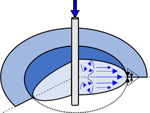
The frequency of these phenomena is especially prevalent in axisymmetric/radial fractures. Near the wellbore, the large flow rates are distributed around a very small circumference, leading to very large Reynolds numbers. These large Reynolds numbers decay quickly as the fluid is dispersed into the fracture, leading to a loss of kinetic energy that must be conserved or dissipated elsewhere in the domain. Large Reynolds numbers also imply the development of turbulence near the wellbore: consider for example the properties of water and a wellbore diameter of 15 cm, then a flow rate of 1 L s $^{-1}$ is sufficient to produce inlet Reynolds numbers in excess of 2000. Figure 1 illustrates the relationship between injection flow rate, injection Reynolds number and wellbore diameter assuming water as the injected fluid. Near the tip, the gradient of aperture is large, which is a significant violation of the Poiseuille assumption, but the flow rate is small, so without investigation it is difficult to estimate the importance of inertial behaviours.
Reynolds number near the wellbore as a function of wellbore diameter and injection flow rate assuming water as the injected fluid. Here  $D$ is the wellbore diameter and $Q$ is the injection flow rate. Even small flow rates can induce very large Reynolds numbers at the wellbore.

The complexity of fluid–fracture interactions at high flow rates is further compounded by the choice of fracturing fluid. More energy is required to pump fluid down the wellbore to the fractures at high flow rates due to the development of turbulence in the wellbore. Consequently, it is common to introduce friction reducers into the fluid to create slickwater (Lecampion & Zia Reference Lecampion and Zia2019; Detournay Reference Detournay2020). Friction reducers disrupt the development of turbulence such that the transition from laminar to turbulent flow is delayed to much higher flow rates at the cost of higher viscosity. Slickwater thus reduces the effects of turbulence at high flow rates but has negligible impact on the inertial behaviour of the fluid.
The primary barrier to investigating these phenomena has been the inability of current models to capture them, particularly inertia. The recently derived GG22 model (Gee & Gracie Reference Gee and Gracie2022) is a newly developed model for fracture flow that is capable of capturing the nonlinear fluid flow behaviours of turbulence, inertia and transience. It is derived by integrating the higher-dimensional incompressible Navier–Stokes equations over the fracture aperture to generate a set of reduced-dimension governing equations that can capture the phenomenon of interest without the computational burden of the full Navier–Stokes equations (Gee & Gracie Reference Gee and Gracie2022). It has been shown that the GG22 model recovers the Poiseuille flow solution under Poiseuille flow conditions, and conserves energy in non-parallel plate geometries where Poiseuille flow does not (Gee & Gracie Reference Gee and Gracie2022).
In this article, we use the GG22 model to establish the impacts of inertia and turbulence on the propagation of axisymmetric hydraulic fractures through numerical simulation of hydromechanically coupled rock mass stimulation. First, we describe the governing equations of the rock mass deformation, fluid flow and hydromechanical coupling. In § 3 we establish the parameters of the hydraulic fracturing scenario under investigation. In § 4, we investigate the solutions to the model problem by varying the fluid physics model, starting with the standard Poiseuille flow solution, then introducing one new phenomenon at a time until we reach the full GG22 fluid model. Next, we discuss the impacts of surface roughness and fracture toughness on the observed results. Last, § 7 investigates how the findings change when the fluid is changed from a Newtonian fluid like water, to a fluid with friction reducers like slickwater. Finally, § 8 summarizes our findings and results.
2. Governing equations
Consider an impermeable rock mass under in situ stresses as illustrated in figure 2(a). Fluid flows through fractures which may propagate through the rock mass. Axisymmetric conditions are assumed, such that the rock mass,  $\varOmega _s$, is considered as a two-dimensional body and the fractures are considered as one-dimensional spaces characterized by an aperture $w(r,t)$ with negligible transverse flow. Typically, fluid flow within fractures is characterized by the Poiseuille flow equation. In this work, we use the GG22 fluid model to explore the phenomena that arise at high flow rates (Gee & Gracie Reference Gee and Gracie2022). The GG22 model is a recently derived model for fracture flow which captures inertial, transient and turbulent fluid behaviours. Similar models have been developed for applications in blood flow through elastic arteries (Olufsen et al. Reference Olufsen, Peskin, Kim, Pedersen, Nadim and Larsen2000) and thin film lubrication (Szeri Reference Szeri1998).
Mathematical domain for an impermeable axisymmetric rock mass under in situ stress with discrete pre-existing fluid-filled fractures. Fracture propagation is controlled by the fracture process zone ahead of the fracture tip which follows a cubic traction–separation law. (a) Mathematical Domain and (b) cubic cohesive traction–separation law.

The GG22 flow model is a two-field model that describes the behaviour of an incompressible fluid with a flux,  $q(r,t)$, and a pressure, $p(r,t)$. The incompressible fluid has density $\rho _f$ and viscosity $\mu$. The governing equations of the GG22 model in axisymmetric form are
 $$\begin{gather} \frac{\partial w}{\partial t} + \frac{1}{r} \frac{\partial }{\partial r} (rq) = 0, \end{gather}$$
 $$\begin{gather}\frac{\partial q}{\partial t} + \frac{1}{r} \frac{\partial}{\partial r} \left( r \alpha \frac{q^2}{w}\right) =- \frac{w}{\rho_f} \frac{\partial p}{\partial r} - \frac{1}{2} \frac{f_D }{w^2} q^2, \end{gather}$$
in which (2.1) is the continuity equation describing the conservation of fluid mass, and (2.2) describes the conservation of fluid momentum. The conservation of momentum equation is comprised of several new terms compared with the Poiseuille flow model. These terms will be referred to as follows:
 $$\begin{gather} \text{transient term: } \frac{\partial q}{\partial t}, \end{gather}$$
 $$\begin{gather}\text{convective term: } \frac{1}{r} \frac{\partial}{\partial x} \left( r \alpha \frac{q^2}{w}\right), \end{gather}$$
 $$\begin{gather}\text{pressure term: } - \frac{w}{\rho_f} \frac{\partial p}{\partial r} , \end{gather}$$
 $$\begin{gather}\text{friction term: } - \frac{1}{2} \frac{f_D }{w^2} q^2. \end{gather}$$
The transient term and the convective term will collectively be referred to as ‘the inertial terms’. While turbulence cannot exist without inertia, the friction term is differentiated because friction is a dissipative phenomenon, while the transient and convective terms capture transformative phenomena. The convective term relates to the convection of momentum by the bulk fluid and enables the conservation of energy of the fluid in response to temporal and spatial changes in aperture (Gee & Gracie Reference Gee and Gracie2022).
In addition to the fields  $q,p$, the conservation of momentum is also a function of two dimensionless coefficients which are functions of the flow regime. First, the momentum correction factor, $\alpha (Re)$, considers the increase in total momentum carried by a non-uniform velocity profile across the aperture. Assuming a parabolic velocity profile in laminar flow and a $1/7$ power-law profile in turbulent flow, the momentum correction factor is defined as
 $$\begin{gather} \alpha = \begin{cases} \frac{6}{5} & \text{if } Re \leq Re_L \\ \frac{64}{63} & \text{if } Re \geq Re_T \end{cases}, \end{gather}$$
 $$\begin{gather}Re = \frac{ \rho_f |\bar{v}| w}{\mu} = \frac{\rho_f|q|}{\mu }, \end{gather}$$
in which  $Re_L$ is the Reynolds number defining the threshold between the laminar regime and the transitional regime, and $Re_T$ is the Reynolds number defining the threshold between the transitional regime and the fully turbulent regime.
The friction factor  $f_D$ accounts for the dissipation of fluid momentum by viscous and turbulent forces. In the laminar regime, dissipation is the result of viscous shear forces, and in the turbulent regime dissipation is caused by both viscous shear and turbulent eddy formation. An empirical relationship is required to determine the friction factor in the turbulent regime, and so the Colebrook–White equation is adopted for simplicity (Colebrook Reference Colebrook1939). The friction factor is thus defined as
 \begin{equation} f_D = \begin{cases} \dfrac{24}{Re} & \text{if } Re \leq Re_L \\ \dfrac{1}{\sqrt{f_D}} =-2\log\left(\dfrac{\epsilon}{7.4w} + \dfrac{2.51}{Re \sqrt{f_D}}\right) & \text{if } Re \geq Re_T \end{cases},\end{equation}
in which  $\epsilon$ is a measure of the surface roughness of the fracture. In the transitional fluid regime, $Re_L < Re < Re_T$, both the momentum correction factor and the friction factor are linearly interpolated. Assuming a Newtonian fluid as the injection fluid (water), the transition from the laminar to the turbulent regime begins at $Re\approx 2000$, while the fully turbulent regime begins at $Re \approx 5000$. The friction factors for water are illustrated in figure 3.
Friction factor as a function of Reynolds number for a standard Newtonian fluid (water) and a fluid enhanced with friction reducers (slickwater).

To reduce the energy required to pump the fluid down the wellbore, it is common to introduce friction reducers into the fluid to create slickwater (Lecampion & Zia Reference Lecampion and Zia2019; Detournay Reference Detournay2020). Friction reducers are long-chain polymers which may be added in small quantities to disrupt the formation of turbulent eddies, delaying the onset of turbulence (Virk Reference Virk1975). The reduction in friction factor reaches a maximum drag reduction (MDR) asymptote at small concentrations (Virk Reference Virk1975). The concentration is dilute, so the density of the bulk fluid remains unchanged, but the viscosity is affected. The fluid becomes non-Newtonian and experiences shear thinning, with the viscosity approaching an asymptotic viscosity after shear degradation. After degradation, the fluid viscosity is approximately constant. It is thus assumed that the slickwater has experienced sufficient shear in the wellbore that it has reached its asymptotic viscosity in the fracture. A Newtonian fluid behaviour is thus assumed in the fracture with an apparent viscosity of 5 mPa s (Habibpour & Clark Reference Habibpour and Clark2017). The friction reducers delay the onset of turbulence from  $Re \approx 2000$ up to $Re \approx 3\times 10^4$. Fully turbulent flow is observed at $Re \approx 5\times 10^5$, so there is a transitional regime between the fully turbulent and MDR regimes. In the MDR regime, which begins at $Re \approx 1000$, the MDR asymptote is correlated with the Reynolds number such that $f_D \propto Re^{-0.7}$ (Virk Reference Virk1975). The friction factor for slickwater is illustrated in figure 3.
In the laminar regime, the friction term simplifies to  $({-12\mu }/{\rho _f w^2}) q$. Under Poiseuille flow conditions, i.e. steady flow through parallel plates, the conservation of momentum equation (2.2) recovers the Poiseuille flow constitutive model,
 \begin{equation} 0 =- \frac{w}{\rho_f} \frac{\partial p}{\partial r} - \frac{12 \mu}{w^2 \rho_f} q \implies q =-\frac{w^3}{12\mu } \frac{\partial p}{\partial r}, \end{equation}
such that flux is a function of the pressure gradient,  $q = f(\,p)$, and the fluid may be described with a single field, $p(r,t)$.
The rock mass is modelled as a quasistatic impermeable linear elastic axisymmetric medium under in situ stress. The equilibrium equation governs the deformation of the rock mass, such that
 $$\begin{gather} 0 = \boldsymbol{\nabla} \boldsymbol{\cdot} \boldsymbol{\sigma} (\boldsymbol{u}) \text{ on } \varOmega_s , \end{gather}$$
 $$\begin{gather}\boldsymbol{\sigma} - \boldsymbol{\sigma}_0 = \mathbb{C} : \varepsilon, \end{gather}$$
in which  $\boldsymbol {u}(r,z,t)$ is the rock mass deformation, $\boldsymbol {\sigma }$ is the axisymmetric Cauchy stress tensor, $\boldsymbol {\sigma }_0$ is the in situ stress tensor, $\mathbb {C}$ is the axisymmetric elasticity tensor and $\varepsilon$ is the axisymmetric linear strain tensor. The rock mass contains fractures defined by an aperture, $w$, which is a function of the deformation of the rock mass. The relationship between aperture and deformation is
 \begin{equation} w = w_0 + \boldsymbol{n_{\varGamma_c}} \boldsymbol{\cdot} \boldsymbol{u} |_{\varGamma_c}, \end{equation}
in which  $w_0$ is some residual aperture in a pre-existing cemented fracture that may arise from surface roughness and $\varGamma _c$ is the fracture surface. The pre-existing cemented fractures are modelled with a traction–separation law such that a quasibrittle cohesive fracture process zone forms ahead of the fracture. A cubic traction–separation law (Tvergaard Reference Tvergaard1990) is adopted, as illustrated in figure 2(b). The traction–separation law is defined as a function of the aperture according to
 $$\begin{gather} t^{coh}(w) = \begin{cases} \frac{27}{4} f_u \varDelta (1 - 2\varDelta + \varDelta^2), & w-w_0 \leq w_c\\ 0, & w-w_0 > w_c \end{cases}, \quad \varDelta = \frac {w-w_0} {w_c} , \end{gather}$$
 $$\begin{gather}w_c = \frac{48}{27} \frac{G_c}{f_u}, \end{gather}$$
in which  $f_u$ is the cohesive strength of the rock mass, $G_c$ is the fracture energy and $w_c$ is the critical aperture which defines the boundary between the cohesive zone and the physical fracture tip. The reopened fracture length is measured as the radial distance from the wellbore to where the aperture exceeds the critical aperture defined by the traction–separation law $w-w_0 >w_c$. The rock mass is therefore subject to tractions on the fracture surfaces such that
 \begin{equation} \boldsymbol{\sigma}\boldsymbol{\cdot} \boldsymbol{n}_{\varGamma_c^\pm} = (-p + t^{coh})\boldsymbol{I} \boldsymbol{\cdot} \boldsymbol{n}_{\varGamma_c^\pm} \text{ on } \varGamma_c^\pm \end{equation}
in which  $\boldsymbol {n}_{\varGamma _c^\pm }$ is the corresponding normal to the positive or negative face of the fracture, $\varGamma _c^\pm$. Fracture propagation in a cohesive-zone model is significantly influenced by fluid lag and vaporization behind the crack tip (Garagash Reference Garagash2019; Liu & Lecampion Reference Liu and Lecampion2021). This effect has been neglected in favour of simplifying the model physics and isolating the effects of the new fluid model but should be otherwise included to capture accurate propagation behaviour.
3. Model problem
In this paper, we consider a single hydraulic fracturing scenario and examine how it reacts to varying fluid physics.
Consider the reopening of a cemented radial fracture with a small residual aperture,  $w_0$ applied uniformly along the cemented fracture. The cemented fracture extends to the end of the computational domain, where a Dirichlet condition is imposed on the pressure such that the pressure is fixed at the far-field hydrostatic pressure of $\bar {p} = \rho _f g h$ in which $g$ is the acceleration due to gravity and $h$ is the fracture depth. The residual aperture allows leak-off through the fracture tip, but as $w_0 \to 0$, the traditional impermeable fracture rock mass solution is recovered. A residual aperture of $w_0 = 5\ \mathrm {\mu }$m is assumed, which results in negligible leak-off in the example below and yield similar results when $w_0 \leq 50$ um. The far-field pressure $\bar {p}$ is placed far enough away from the fracture tip that the effects of injection do not reach the far-field boundary and the flux through the far-field boundary is negligible. The surface roughness of the fracture faces is conceptualized as asperities which are compressed in the initial stress state and decompress as the fracture opens. The maximum relative roughness is initially set to $\epsilon / w = 0.99$ and decreases as the fractures open. The asperities are set to a maximum roughness of $\epsilon = 0.5$ mm. The selected parameters for this model problem are summarized in table 1
Model problem simulation parameters.

The cemented radial fracture exists within an impermeable granite rock mass at a depth of  $h=2000$ m and a minimum in situ stress of $\sigma _0 = 25$ MPa. The rock mass has a tensile strength of $F_u =10$ MPa, an elastic modulus of $E = 60$ GPa and Poisson's ratio of $\nu = 0.25$. The dimensions of the computational domain are illustrated in figure 4. The computational domain is symmetrical along the axis of the fracture.
Computational domain for the reopening of a cemented radial fracture.

Fluid is injected into a wellbore with a diameter of  $D = 15$ cm. The injection rate $Q_o(t)$ is specified in terms of the injection Reynolds number, $Re = {\rho _f \bar {q}}/{\mu } = {\rho _f Q_o}/{\mu {\rm \pi}D}$. Injection rates of $Re = 10$ up to $Re = 2\times 10^5$ are considered. Two injection fluids are considered: water with a density of $\rho _f = 1000$ kg m $^{-3}$ and a viscosity of $\mu = 1\ {\rm mPa} \ {\rm s}$; and slickwater with a density of $\rho _f = 1000$ kg m $^{-3}$ and a viscosity of $\mu = 5\ {\rm mPa} \ {\rm s}$. The maximum injection Reynolds number corresponds to a maximum injection flow rate of 36 b.p.m. ( $5.75\ {\rm m}^3\ {\rm min}^{-1}$, 96 L s $^{-1}$) for water and 180 b.p.m. ( $28.75\ {\rm m}^3\ {\rm min}^{-1}$, 480 L s $^{-1}$) for slickwater. The injection rate is applied with a linear ramp over the first 6 s, and a constant injection rate for the rest of the simulated time as illustrated in figure 5. The fracture propagation is simulated for a total of 60 s.
Applied injection rate over the simulated injection time.

The model problem is solved numerically using a fully coupled monolithic mixed finite element method–finite volume method. Finite elements are used to discretize the rock mass, while finite volumes are used to discretize the fracture. The reader is referred to Gee & Gracie (Reference Gee and Gracie2023) for details on the derivation, implementation and verification of the numerical method employed here. The injection of a fixed flow rate into a radial fracture with turbulent flow leads to a large but finite pressure gradient at the wellbore (Lecampion & Zia Reference Lecampion and Zia2019), provided the wellbore radius is finite. Figure 6 illustrates the computational mesh employed for these simulations. A very fine mesh is required near the inlet to resolve the pressure gradient at the wellbore. Past the wellbore, a coarser mesh is employed along the expected length of the fracture, and the coarsest mesh is applied along the exterior edges of the domain. The fluid volumes follow the rock mass mesh with volumes exactly aligned to the element edges along the fracture face.
Computational mesh with element area ( ${\rm m}^2$), illustrating the refinement required near the wellbore to resolve the pressure gradient.

A zero-toughness fracture case is considered first, such that the fracture propagation is restricted only by the resistance of the initial residual aperture. In this case, the physical tip is assumed to be the coordinate where  $w > w_0$. Next, various fracture toughnesses are considered using the cubic cohesive zone traction–separation law.
4. The effects of turbulence and inertia
In this section, we will examine the behaviour of the fracture propagation problem described in § 3. To isolate the fluid behaviour, a zero-toughness fracture is considered ( $G_c = 0 \ {\rm J}\ {\rm m}^{-2}$). We will consider the problem with four layers of fluid physics by modifying the conservation of momentum equation (2.2). First, we will consider the problem using the standard Poiseuille flow model, which assumes steady laminar flow through a constant aperture. Next, we will upgrade the friction term to capture turbulent flow, but neglect the inertial terms introduced by the GG22 model. Third, we will assume laminar flow, but introduce the inertial terms into the conservation of momentum. Last, we will consider the full GG22 conservation of momentum equation. By layering the physics one at a time, we will be able to isolate how each term affects the solution and determine the flow rate threshold at which each layer becomes relevant. It is assumed throughout this section that a standard Newtonian fluid (water) is used as the fracturing fluid, and friction reducers have not been introduced.
4.1. The Poiseuille flow solution
First, we discuss the standard Poiseuille flow solution as a baseline case for the model problem. The Poiseuille flow model is the standard assumption for most fracture flow simulations. Steady laminar flow is assumed and the conservation of momentum equation (2.2) simplifies to
 \begin{equation} 0 =- \frac{w}{\rho_f} \frac{\partial p}{\partial r} -\frac{12\mu}{\rho_f w^2} q, \end{equation}
which can be rearranged as a constitutive relationship between flux and pressure such that
 \begin{equation} q =- \frac{w^3}{12 \mu } \frac{\partial p}{\partial r}. \end{equation}
Figure 7 illustrates the pressure at the wellbore. There is an initial peak pressure associated with the reopening of the fracture, followed by a monotonic decrease in pressure. Within the constitutive equation there are two competing processes: fracture lengthening and fracture opening. Lengthening requires an increase in pressure at the wellbore to propel the fluid a farther distance. Opening decreases the pressure at the wellbore as the resistance to fluid flow decreases. The injection pressures indicate that fracture opening generally dominates, but at higher injection rates, the pressure decreases more slowly over time as fracture lengthening has a greater contribution.
Wellbore pressure from injecting water at various flow rates with a Poiseuille flow model. The Poiseuille flow solution shows a spike in pressure to reopen the fracture, then decreases over time.

Figure 8(a) illustrates the pressure along the fracture after  $60$ s of injection at the highest tested injection rate of $Re = 2\times 10^5$. The pressure decreases monotonically until the fracture tip. There is a discontinuity in the pressure gradient at the fracture tip as the residual fracture aperture allows fluid to flow ahead of the reopened fracture tip. Though the pressure gradient is large, the aperture is small, and the flow towards the tip from the cemented fracture is negligible compared with that from the reopened fracture. In the example, the tip behaviour does not appear to be influenced significantly by tip leak-off. Farther ahead of the fracture tip, the pressure slowly returns to the far-field pressure. Figure 8(b) illustrates the aperture along the fracture. The aperture decreases monotonically and continuously. There is a discontinuity in the aperture gradient at the tip.
Pressure and aperture along the fracture with a Poiseuille flow model after 60 s of injecting water at a rate of  $Re = 2\times 10^5$. (a) Pressure decreases along the fracture and a sharp decrease in pressure is observed at the fracture tip and (b) aperture decreases along the fracture.

4.2. The effects of turbulence
Next, we consider replacing the Poiseuille constitutive equation with a turbulent friction term. Given that most fracture flow simulation tools are developed for Poiseuille flow, the inclusion of the inertial terms in the conservation of momentum equation are intrusive and require significant modifications. The implementation of a turbulent friction term without the inertial terms is therefore an attractive prospect for capturing the effects of turbulence with minimally intrusive implementation.
The equation for conservation of momentum (2.2) becomes
 \begin{equation} 0 =- \frac{w}{\rho_f} \frac{\partial p}{\partial r} -\frac{f_D(q)}{ w^2} q^2, \end{equation}
which may be rearranged into a nonlinear constitutive equation
 \begin{equation} q =- \frac{w^3}{\rho_f f_D(q)\cdot q} \frac{\partial p}{\partial r}. \end{equation}
 Figure 9 illustrates the pressure at the wellbore for increasing flow rates. There is an initial local peak pressure associated with the opening of the fracture, as observed in the Poiseuille flow case. Unlike the Poiseuille flow case, at sufficiently high flow rates to induce turbulence, the required pressure to maintain the injected flow rate increases due to the resistance created by turbulence. With a turbulent flow model, the pressure required to maintain a flow of  $Re=2\times 10^5$ is approximately four times greater than with the Poiseuille flow model.
Wellbore pressure from injecting water at various flow rates considering a turbulent model but neglecting inertia. The inclusion of turbulence requires much higher pressures to achieve the same injection rates. Large pressures are required to open the fracture, then pressure decreases, but the increasing flow rate increases resistance to flow resulting in a peak pressure at 6 s when the flow finishes ramping up to its prescribed injection rate.

Figure 10(a) illustrates the pressure along the fracture compared with the Poiseuille flow case after 60 s at the highest tested injection rate of  $Re = 2\times 10^5$. There is a region of significantly elevated pressure near the wellbore extending up to 5 m along the fracture radius. Farther along the fracture, the fluid returns to laminar flow and the pressures are similar to the Poiseuille flow profile. Figure 10(b) illustrates the aperture distribution along the fracture. The elevated pressures near the wellbore create a region of increased aperture, with an increase of 90 % at the wellbore in this case. The aperture decreases monotonically along the fracture, but the curvature of the aperture changes around 20 m. To conserve the total injected volume, the aperture farther along the fracture is slightly smaller and the overall fracture length is slightly shorter than the Poiseuille flow case.
Pressure and aperture along the fracture with a turbulent flow model that neglects inertia after 60 s of injecting water at a rate of  $Re = 2\times 10^5$. (a) A large increase in pressure is observed near the wellbore to overcome the turbulent resistance. The flow returns to laminar flow farther along the fracture and the solution resembles the Poiseuille flow solution after 10 m and (b) the large increase in pressure at the wellbore causes a large increase in aperture (a 90 % increase in this simulation). To preserve the total injected volume, the fracture is slightly shorter than the Poiseuille case.

4.3. The effects of inertia
Next, we consider the behaviour of fracture growth when we introduce the inertial terms but maintain the laminar flow assumption from Poiseuille flow. The conservation of momentum equation (2.2) becomes
 \begin{equation} \frac{\partial q}{\partial t} + \frac{1}{r} \frac{\partial}{\partial r} \left(r \frac{\alpha}{w} q^2\right) =- \frac{w}{\rho_f} \frac{\partial p}{\partial r} -\frac{12\mu}{\rho_f w^2} q, \end{equation}
and cannot be rearranged into a constitutive equation. It remains a separate coupled governing partial differential equation which must be simultaneously solved.
Figure 11 illustrates the pressure at the wellbore for increasing injection rates. At sufficiently high flow rates, the inertial terms induce positive pressure gradients and therefore the pressure at the wellbore required to maintain the injection flow rate decreases. There is an initial peak positive pressure associated with reopening the fracture, after which as the flow rate increases, the wellbore pressure drops precipitously. The pressures illustrated in figure 11 are gauge pressures relative to the hydrostatic pressure, and so the negative gauge pressures are still positive absolute pressures and cavitation is not a concern.
Wellbore pressure from injecting water at various flow rates considering a model including inertial terms but assuming laminar flow. A reduction in pressure is observed as the decreasing fluid velocity creates a positive pressure gradient at the wellbore. Pressure here is measured relative to the hydrostatic pressure, so total pressure remains positive.

The dominant term behind the negative pressure is the continuity term. Consider the case of injection at a constant rate into a set of radial parallel plates (constant  $w$). In this case, the steady-state solution for flux takes the form, $q\propto 1/r$. The velocity of the fluid is proportional to the flux, $q = \bar {v} w$, where $\bar {v}$ is the average fluid velocity across the cross-section. Thus, as the flux moves away from the wellbore, the velocity of the fluid must decrease to maintain continuity. When the fluid velocity is decreasing, that kinetic energy must be transformed into potential energy or be dissipated. If the friction term cannot dissipate the excess kinetic energy faster than the rate at which the fluid is decelerating, that excess energy is transformed into potential energy in the form of an increase in fluid pressure. The result is the development of a positive pressure gradient at the wellbore despite the positive direction of flow. The negative pressure causes the aperture to decrease, which then increases the friction term, leading to non-monotonic interactions at high $Re$.
$Re$.
Figure 12(a) illustrates the pressure along the fracture when considering the inertial terms with laminar flow compared with the Poiseuille flow solution after 60 s at the highest tested injection rate of  $Re = 2\times 10^5$. Similar to the turbulent flow solution, there is a region of deviation from the Poiseuille flow solution near the wellbore, but it does not extend as far as in the turbulent solution. Approximately 1 m along the fracture, the fluid returns and the pressures are well approximated by the Poiseuille flow profile. Figure 12(b) illustrates the aperture profile along the fracture. The negative pressures at the wellbore induce a decrease in the aperture at the wellbore, which also increases the velocity and thereby exacerbates the influence of the convective term. To conserve the overall injected volume, the fracture is slightly longer than the Poiseuille flow case and the apertures near the tip are slightly larger.
Pressure and aperture along the fracture with a model that includes inertial terms but assumes laminar flow after 60 s of injecting water at a rate of  $Re = 2\times 10^5$. (a) The slowing fluid introduces a positive pressure gradient near the wellbore and creates negative pressures. The effect is localized near the wellbore and the solution returns towards the Poiseuille flow solution within 1 m and (b) the negative pressures cause a decrease in the aperture near the wellbore. To accommodate the total injected volume, the fracture length must increase.

4.4. The combined effects of inertia and turbulence
Based on the results of the previous sections, we can observe that the two phenomena of inertia and turbulence are in conflict. One seeks to increase pressure and decrease crack length, while the other seeks to decrease pressure and increase crack length. Only by combining the two phenomena into a single model can we observe the true fluid behaviour. Thus, we now consider the full GG22 flow model and solve the conservation of momentum equation as
 \begin{equation} \frac{\partial q}{\partial t} + \frac{1}{r} \frac{\partial}{\partial r} \left(r \frac{\alpha}{w} q^2\right) =- \frac{w}{\rho_f} \frac{\partial p}{\partial r} -\frac{f_D(q)}{ w^2} q^2. \end{equation}
 Figure 13 illustrates the pressure at the wellbore for increasing injection rates. The overall form of the pressure curves is similar to the turbulent-only solution in figure 9, but the peak pressures at  $t=6$ s are reduced. We therefore observe that the turbulent friction factor is dominant at lower $Re$ and the effects of the inertial terms do not manifest until higher $Re$, though it has significant effects on the pressure (a reduction of 5 MPa at $t=6$ s for $Re = 2\times 10^{5}$).
Wellbore pressure from injecting water at various flow rates considering a model with turbulent and inertial terms. In general, the turbulent solution is dominant, however, the influence of the negative pressures from the inertial terms significantly reduce the pressures.

Figure 14(a) illustrates the pressure along the fracture after 60 s at the highest tested injection rate of  $Re = 2\times 10^5$. The full model pressure generally aligns with the turbulent-only model, though pressures are reduced up to 20 % in the vicinity of the wellbore. Figure 14(b) illustrates the aperture along the fracture. The increase in aperture from turbulence reduces the influence of inertia, as the increased aperture at the wellbore results in a lower fluid velocity to maintain the prescribed wellbore flux ( $q = \bar {v} w$). The decrease of pressure at the wellbore does not translate directly to the same decrease in aperture, and though it is reduced compared with the turbulent-only model, the reduction is small. We attribute this difference to the fact that aperture and pressure are no longer directly correlated through a constitutive equation and instead are now indirectly correlated through a partial differential equation. The crack length is similar to the turbulent-only model. In all cases, the changes in crack length are very small, of the order of $10^{-3}$ compared with the overall fracture length. Compared with existing turbulent and inertial flow studies, Zia & Lecampion (Reference Zia and Lecampion2017) conclude by dimensional analysis that the inertial terms are always negligible. In the context of the fracture tip and the asymptotic fracture propagation solution, our results do agree with this conclusion. However, our results indicate that this statement is not true when concerned with the near-wellbore behaviour. While turbulence is dominant using water, the reduction in pressure at high flow rates is significant. Thus, for the prediction of near-wellbore behaviours with water as the injection fluid (such as important operating parameters like injection pressure), turbulent behaviour is dominant but inertial terms are not negligible.
Pressure and aperture along the fracture with turbulent and inertial terms after 60 s of injecting water at a rate of  $Re = 2\times 10^5$. (a) Turbulence is dominant over the inertial terms in the pressure solution but inertia reduces the pressures within the first metre and (b) though the differences in pressure are significant when comparing turbulent solutions with and without inertia, the translation to aperture is more modest. The inertial turbulent solution shows only marginally smaller apertures compared with the full turbulent model.

Figure 15 illustrates how the various fluid models affect the distribution of stress in the rock mass. The Poiseuille flow model generates a single stress concentration at the fracture tip. Introducing turbulence generates increased fluid pressure at the wellbore, which in turn increases the stresses in the rock mass at the wellbore. Including inertia but neglecting turbulence causes the pressure to decrease at the wellbore and restricts the wellbore aperture. Echoing the fluid pressure behaviours, the stress concentration induced by the inertial terms is more localized than the stress concentration induced by turbulence. The full GG22 fluid flow model shows stress concentrations at the wellbore, but the magnitude and size of the concentrations are reduced due to the influence of inertia compared with the turbulent-only model.
Rock mass stresses and fluid pressures for an injection rate of  $Re = 2\times 10^5$ with water for various flow models after 60 s of injection. Displacements are scaled $\times 2000$. (a) Poiseuille flow model: a stress concentration is observed near the fracture tip. (b) Turbulent-only flow model: the increased fluid pressure at the wellbore creates a stress concentration at the wellbore. (c) Inertia-only flow model: the decreased fluid pressure at the wellbore creates a stress concentration at the wellbore. (d) Full GG22 flow model: the interaction of turbulence and inertia decrease the magnitude of the stress concentration at the wellbore compared with the turbulent only model.

Figure 16(a) illustrates the pressure at the wellbore after 60 s of injection for various  $Re$. The full flow model deviates from the Poiseuille flow model as soon as turbulence is induced at $Re \approx 2 \times 10^3$. The full model and the turbulent-only model remain similar up to $Re \approx 2 \times 10^4$, after which the effects of inertia manifest and the full model deviates from the turbulent-only model. Figure 16(b) illustrates the aperture at the wellbore after 60 s of injection time. The full model deviates from the Poiseuille flow model as soon as turbulence is introduced, but the effects of inertia are more modest and differences with the turbulent-only model are small.
Pressure and aperture at the wellbore after 60 s of injecting water at a various flow rates. (a) Comparison of wellbore pressures after 60 s. The full physics behaviour departs from the Poiseuille flow solution by  $Re = 5000$. The inclusion of turbulence increases the injection pressure by a factor of approximately four. Including turbulence but neglecting inertia overestimates the required pressure by up to 20 % in the tested range and (b) turbulence increases the pressure at the wellbore which in turn increases the aperture. Despite the large pressure differences that arise by neglecting inertia, this does not translate to the same difference in aperture. Smaller apertures are observed, but the difference is more modest.

Figure 17 illustrates the fraction of inertial and turbulent forces to the total pressure drop observed along the fracture. As the inertial and turbulent forces are localized to the wellbore (approximately 2 m or 13 wellbore diameters), this fraction indicates the ratio of entrance losses to the total pressure loss along the fracture. This fraction is calculated as
 \begin{equation} \text{entrance loss fraction} = \frac{\Delta p_{Full} - \Delta p_{PF}}{\Delta p_{Full}}, \end{equation}
in which  $\Delta p_{Full}$ is the difference between the wellbore pressure from the full GG22 model and the far-field pressure, and $\Delta p_{PF}$ is the difference between the wellbore pressure from the Poiseuille flow and the far-field pressure. We observe that the majority of the pressure loss that occurs along the fracture is attributable to entrance losses. The fraction of entry losses increases rapidly after turbulence is induced at $Re = 2000$, surpassing 0.5 by $Re = 5000$. It approaches an asymptote of 0.93 at higher $Re$, though the exact value of this asymptote is likely unique to this specific problem set-up. Crack length and injection time do not appear to have a significant impact on the ratio. These results imply that entrance losses, a phenomenon observed experimentally (Lecampion et al. Reference Lecampion, Desroches, Jeffrey and Bunger2017) and often attributed to wellbore perforations, may be described wholly or in part by turbulent and inertial forces which develop near the wellbore due to high $Re$ flow conditions. However, true near-wellbore behaviour is a complicated phenomenon, confounded by the flow in the wellbore, the effects of perforations and near-wellbore tortuosity (Bunger & Lecampion Reference Bunger and Lecampion2017). This model does not capture all these near-wellbore effects but suggests that these effects must be considered in combination with inertia and turbulence to fully capture the near-wellbore behaviour. These results imply that near-wellbore behaviour, in addition to turbulent flow in the well, may govern the wellbore pressure and thus the power required to inject fluid at these high flow rates into the fractures.
Relative contribution of turbulent and inertial forces to the total pressure difference along the fracture. Water is assumed as the injection fluid. The contribution of turbulent and inertial forces to the pressure difference rapidly increases once turbulence is induced and eventually converges towards an asymptote of 0.93. Crack length  $L$ seems to have little effect on the contribution in this case, but may have a larger effect in longer fractures.

With regard to the implications and importance of inertia to the overall fracture propagation, Zia & Lecampion (Reference Zia and Lecampion2017) conclude by dimensional analysis that the inertial terms are always negligible, while Garagash (Reference Garagash2006) concludes that inertial terms are only important in the early-time solution. We have shown that inertia is primarily a near-wellbore effect in fracture propagation, so in this context we can recast the conclusions of Garagash (Reference Garagash2006) to understand that the conclusion that inertial terms are only important in the early-time is analogous to assuming that near-wellbore effects become negligible as the fracture length increases. In the context of the overall fracture length, our results agree with this conclusion, and the scaling arguments presented by Garagash (Reference Garagash2006) may be used to estimate the importance of inertia to the overall fracture propagation. However, inertia is a phenomenon that occurs relative to the forces over a cross-section, independent of the fracture length. Thus, when concerned with near-wellbore behaviour, the inertial effects are not negligible at high flow rates. Furthermore, the total pressure drop along the fracture appears to be dominated by near-wellbore behaviour caused by turbulent and inertial effects. By neglecting this combination of effects near the wellbore, it may be possible to predict the overall fracture length, but considerably under- or over-estimate the amount of power (product of flow rate and pressure) required to generate a fracture of that length.
Based on these observations, the authors make the following recommendations for the simulation of axisymmetric fractures with Newtonian hydraulic fracturing fluids. For injection flow of  $Re < 2000$, the Poiseuille flow model appears to be adequate. For injection flow rates in the range of $2 \times 10^3 \leq Re \leq 2 \times 10^4$, one should include the effects of turbulence but may neglect the effects of inertia with minimal error. For injection flow rates $Re > 2 \times 10^4$, one should include both the effects of inertia and turbulence. If one is only interested in predicting crack lengths and apertures, it appears that one could apply a higher upper bound on the range of applicability of the turbulent-only model at the cost of over-predicting the pressures. For wellbore diameters of 10, 15 and 20 cm (4, 6, 8 in.), these thresholds correspond to flow rates of 0.65, 0.98, 1.3 L s $^{-1}$ (0.24, 0.36 and 0.48 b.p.m.) for the onset of turbulence effects ( $Re \geq 2\times 10^3$) and 6.5, 9.8, 13 L s $^{-1}$ (2.4, 3.6 and 4.8 b.p.m.) for the onset of inertial effects ( $Re \geq 2\times 10^4$) assuming water as the injected fluid.
While the results presented herein are discussed in terms of the dimensionless  $Re$, the system is nonlinear so the magnitudes of flow rate and wellbore diameter will have some effect on the results presented. However, the differences in the size of the wellbore that occur in practice are small, and the flow rates pumped through those wellbores scale with wellbore size, so we expect qualitatively similar behaviour without significant differences when considering wellbores sizes other than the 15 cm adopted here. Furthermore, these results and recommendation thresholds assume water without additives as the injected fluid. The use of additives in the injected fluid, such as slickwater, which reduce drag and affect the transition from laminar to turbulent flow will influence these thresholds. The effects of additives are discussed further in § 7.
5. The effects of surface roughness
The friction factor as determined by the Colebrook–White equation is a function of two terms: the relative roughness of the fracture surfaces compared with the aperture, and the Reynolds number. At the Reynolds numbers considered in this analysis, the friction factor is controlled primarily by the surface roughness term. As the flux is not constant along the radius, neither is the friction factor, and the asymptotic friction factor is only reached near the wellbore. As the Colebrook–White equation is primarily applicable in the context of pipe flow, it is important to question the influence of the assumed empirical relationship on the results we are interpreting. The surface roughness we have specified is at the high end of the range of applicability of the Colebrook–White equation, and as rock mass fractures are highly heterogeneous and uneven, the friction factor is likely to be even greater in reality. Thus, the onset of turbulence effects is likely under-estimated by the current study. To further emphasize the need to consider these effects, let us examine the results using a lower surface roughness.
We consider a very smooth fracture surface with a roughness up to  $\epsilon = 10\ \mathrm {\mu }$m and compare it with the earlier results with a surface roughness up to $\epsilon = 500\ \mathrm {\mu }$m, which is still small compared with a real rock mass fracture. Figure 18 illustrates the wellbore pressures after 60 s of injection time for high and low surface roughness. Both show significantly different behaviour from the Poiseuille flow model and similar trends: they depart from the Poiseuille flow solution as soon as turbulence is induced, and the influence of the inertial terms manifests at higher $Re$ than the influence of turbulence. The influence of the inertial terms is greater in the low roughness case as the smaller pressures create smaller apertures and therefore higher fluid velocities and greater inertial effects. The departure of the full model from the turbulent-only model therefore occurs at lower $Re$ than the high roughness case. Nevertheless, it shows that even with smooth fracture faces, the influence of turbulence and inertia cannot be neglected, and with larger roughnesses the findings presented herein are only reinforced.
The influence of the surface roughness term on wellbore pressure after 60 s of injection. Water is assumed as the injection fluid.

6. The effects of fracture toughness
Thus far, we have considered the reopening of a zero-toughness fracture for the model problem described in § 3. In this section we will introduce fracture toughness through a cohesive fracture process zone ahead of the fracture with a cubic traction separation law (Tvergaard Reference Tvergaard1990).
Consider the definitions of the dimensionless viscous and toughness coefficients for a penny-shaped fracture defined by Detournay (Reference Detournay2004). The dimensionless viscous storage coefficient is proportional to
 \begin{equation} \mathcal{M} \propto \mu \left( \frac{ E^{13} Q_o^3 }{K_{Ic}^{18} t^2} \right)^{1/5}\propto \mu \left( \frac{ E^{13} Q_o^3 }{G_c^9 t^2} \right)^{1/5} \propto \left( \frac{ E^{13} \mu^8 Re^3 }{G_c^9 t^2 \rho_f^3} \right)^{1/5}, \end{equation}
while the dimensionless toughness coefficient is proportional to
 \begin{equation} \mathcal{K} \propto K_{IC} \left( \frac{t^2}{\mu^5 Q_0^3 E^{13}} \right)^{{1/18}} \propto G_c^{{1}/{2}} \left( \frac{t^2}{\mu^5 Q_0^3 E^{13}} \right)^{{1/18}} \propto G_c^{{1}/{2}} \left( \frac{ \rho_f^3 t^2}{\mu^8 Re^3 E^{13}} \right)^{{1/18}}, \end{equation}
where  $K_{IC}$ is the mode I fracture toughness of the rock mass. The two dimensionless coefficients are inversely proportional to each other, such that one decreases as the other increases. The viscous and toughness coefficients $\mathcal {M}$ and $\mathcal {K}$ are derived from fracture propagation solutions assuming Poiseuille flow and linear elastic fracture mechanics. These scaling coefficients are not directly comparable to the models considered here which use the GG22 flow model and a cohesive fracture model and are instead used in analogy only.
The toughness coefficient is proportional to time and inversely proportional to the Reynolds number. This implies that the fracture propagation in axisymmetric fractures starts as viscous-dominant propagation and transitions to toughness-dominant propagation as the fracture length increases (Detournay Reference Detournay2004). As the toughness coefficient is inversely proportional to the Reynolds number, it becomes less relevant at higher injection rates and viscous effects become stronger. We therefore hypothesize that inertial and turbulent effects will not manifest in toughness-regime propagation solutions for axisymmetric fractures.
Figure 19(a) illustrates the fracture length and figure 19(b) illustrates the wellbore pressure as functions of the injection rate after 60 s of injection with the GG22 and Poiseuille flow models for fracture energies of  $G_c = 0, 250, 500 \ {\rm J}\ {\rm m}^{-2}$. The fracture energies considered are very high for a brittle rock formation, but we consider high fracture energies to examine the asymptotic case and increase the toughness coefficient at high injection rates. No significant differences are observed in fracture length between the fluid models, but higher fracture toughness is correlated with shorter fractures. This implies that the fracture length in the model problem considered here is governed primarily by fracture toughness and the near-wellbore physics have minimal effect on the fracture length. However, significant differences in wellbore pressure are observed between the two models and the wellbore pressure is governed by the near-wellbore effects of turbulence and inertia. This follows the conclusions drawn in § 4.4, that while tip mechanics govern the fracture length, the amount of pumping power required to generate a fracture of that length may be significantly over- or under-estimated without the inclusion of turbulence and inertia.
Fracture length and pressure at the wellbore for varying fracture energies ( $G_c$, J m $^{-2}$). Water is assumed as the injection fluid. Negligible differences in fracture length are observed despite significant differences in injection pressure. (a) Fracture length after 60 s. No significant difference in fracture length is observed between the Poiseuille and GG22 flow models and (b) injection pressure after 60 s. At low $Re$, the pressure is correlated by the fracture toughness. At high $Re$, the pressure is governed by the fluid resistance.

7. The effects of friction reducers (slickwater)
It is common in hydraulic fracturing treatments to use slickwater to reduce the energy of pumping the fracturing fluid down the wellbore (Lecampion & Zia Reference Lecampion and Zia2019; Detournay Reference Detournay2020). The polymers introduced in slickwater delay the onset of turbulent flow from  $Re \approx 2\times 10^3$ to $Re \approx 3\times 10^4$, which has significant effects on the fluid behaviour (Virk Reference Virk1975) at the cost of higher viscosity, $\mu = 5\ {\rm mPa}\ {\rm s}$ (Habibpour & Clark Reference Habibpour and Clark2017). In this section we examine how turbulent and inertial effects manifest in the zero-toughness fracture problem ( $G_c = 0 \ {\rm J}\ {\rm m}^{-2}$) described in § 3.
Figure 20 illustrates the pressure at the wellbore for increasing injection rates. While the behaviour is different from the water cases, the various terms in the governing equation produce the same effects. In the laminar regime, water and slickwater exhibit the same behaviour. As the slickwater enters the MDR regime ( $10^3 < Re < 3\times 10^4, f_D \propto Re^{-0.7}$), we observe a reduction in pressure at the wellbore. Much like the case of inertia without turbulence discussed in § 4.3, the slowing fluid supplies energy faster than it is dissipated by friction, so a positive pressure gradient develops at the wellbore. The delayed onset of turbulence implies that even at higher $Re$, inertial effects dominate the solution.
Injection pressure for various injection rates with slickwater considering the full GG22 model. The higher viscosity of slickwater implies larger flow rates than water at the same Reynolds number, creating inertia dominant flow and producing a positive pressure gradient at the wellbore which reduces pressure.

Thus, while turbulence was the dominant effect at lower  $Re$ in pure water and inertia did not become important until higher $Re$, we draw the opposite conclusion in slickwater. In slickwater, inertia is the dominant effect at lower $Re$ and turbulence only becomes important at higher $Re$. Figure 21(a) illustrates the pressure at the wellbore after 60 s of injection for various $Re$ and models with slickwater. While the MDR regime begins at $Re > 1000$, we observe that Poiseuille is a reasonably good approximation until $Re \approx 5\times 10^3$. At $Re > 5\times 10^3$, after which inertia creates deviations from the Poiseuille flow solution. figure 21(b) compares the wellbore pressures for the full GG22 model between water and slickwater. The higher viscosity of slickwater implies that a larger flow rate of slickwater is required to produce the same Reynolds number, thus at low $Re$ the slickwater pressures are increased compared with water. The larger flow rates increase the inertial effects, causing inertia to be the dominant mechanism in the wellbore pressure at large flow rates. In a similar but inverted case to water, turbulence and inertia are in opposition. Each mechanism moderates the other at high Reynolds numbers and turbulence reduces the magnitude of wellbore pressure by 50 % in high $Re$ slickwater flow. Turbulence leads to deviations from the inertia-only solution at $Re > 2\times 10^4$. Figure 21(c) illustrates the wellbore pressures for various models as a function of flow rate. Slickwater successfully reduces the power needed to pump fluid down the wellbore at the same flow rate, and inertial effects are not observed until flow rates of 0.7 ${\rm m}^3\ {\rm min}^{-1}$ (11 L s $^{-1}$, 4.5 b.p.m.).
Wellbore pressure after 60 s of injection with water and slickwater. (a) Slickwater wellbore pressure for with various models as a function of  $Re$. (b) Water and slickwater GG22 wellbore pressure as a function of $Re$. (c) Water and slickwater GG22 wellbore pressure as a function of $Q$.
$Q$.

Figure 22(a) illustrates the pressure along the fracture after 60 s of injection at the highest tested injection rate of  $Re = 2\times 10^5$ for both water and slickwater. Figure 22(b) illustrates the aperture along the fracture. The larger viscosity of slickwater requires a larger flow rate to generate the same Reynolds number, which creates longer fractures with larger apertures and higher pressures away from the wellbore. The shape of the solution is similar to the inertia-only model with water. The amplified inertial effects increase the aperture of the fracture near the tip. As the model is nonlinear, the $5\times$ increase in viscosity and flow rate correspond to an approximately $5 \times$ increase in fracture volume, but only a $2\times$ increase in pressure.
Comparison of pressure and aperture along the fracture with water and slickwater after 60 s of injection with an injection rate of  $Re = 5\times 10^4$. (a) Pressure in the fracture is greater and inertial effects dominate near the wellbore with slickwater and (b) the larger flow rate results in a larger fracture with an area of reduced aperture near the wellbore due to inertial effects.

The trends observed with slickwater do not substantially change when a fracture toughness is reintroduced. Similar trends to those observed with water in § 6 are observed: at the flow rates large enough to induce inertial and turbulent effects, the fracture propagation is pushed away from toughness dominant propagation and is instead dominated by fluid behaviours.
8. Conclusions
We have investigated for the first time the effects of inertia and turbulence on the hydraulic stimulation of fractured rock masses using the GG22 model, with effects manifesting for both water and slickwater treatments. The phenomena of inertia and turbulence are significant near the wellbore where the flux is greatest and are responsible for the majority of the total pressure loss along the fracture. This suggests that inertial and turbulent forces may provide a more accurate description for entrance losses, an experimentally observed phenomenon which was previously accounted for in an empirical manner. As the flow disperses into the fracture, laminar flow is recovered and the Poiseuille flow is well-suited to modelling the flow behaviour. At the fracture tip, no inertial or turbulent effects are observed due to the low flow rates. We observe that the fracture length is primarily governed by fracture toughness and tip mechanics, while injection pressure is primarily governed by the near-wellbore effects of turbulence and inertia. Neglecting to account for these near-wellbore physics may lead to significant over- or under-estimation of the amount of pumping power required to generate a fracture of a given length.
Using water as the injected fluid, the development of turbulence leads to significant increases in the injection pressure and the formation of an area of increased aperture near the wellbore relative to the Poiseuille flow solution. These significant changes in wellbore aperture and pressure translate minimal changes in overall crack length. While turbulence increases wellbore pressure, inertia at high flow rates reduces wellbore pressure. A model which only includes turbulence leads to an overestimation of the injection pressure at high Reynolds numbers. Turbulence is generally the dominant phenomenon, causing deviations from the Poiseuille flow solution as soon as it is induced, at an injection Reynolds number of  $Re \approx 2\times 10^3$, approximately corresponding to a flow rate of 0.4 b.p.m. Inertial effects do not manifest until higher Reynolds numbers, deviating from a turbulent-only model at Reynolds numbers of $Re \approx 2\times 10^4$, approximately corresponding to a flow rate of 4 b.p.m. Inertial and turbulent forces manifest primarily within 2 m of the wellbore (13 wellbore diameters). Increasing surface roughness exacerbates turbulent effects and delays the onset of inertial effects.
Using slickwater as the injected fluid, we observe the opposite trend. Slickwater delays the onset of turbulence but not inertia, so inertia induces reduces the wellbore pressure relative to the Poiseuille flow solution. Inertial effects in slickwater begin to manifest at a Reynolds number of  $Re \approx 5\times 10^3$ (approximate flow rate of 5 b.p.m.). Turbulent effects in slickwater begin to manifest at $Re \approx 2\times 10^4$ (approximate flow rate of 18 b.p.m.).
Based on the observations in this work, any simulation of flow in a radial fracture from a wellbore using water should at the very least include turbulent behaviour. The threshold for the departure from the standard Poiseuille flow solution is low, and the change in fracture geometry and flow behaviour is large. The threshold to induce inertial effects in water is also relatively low, and simulations dealing with higher injection Reynolds numbers should consider the implementation of inertia to capture the complete fluid behaviour. While Poiseuille flow is better at approximating slickwater behaviour, any simulation of flow in a radial fracture from a wellbore using slickwater should consider including inertial behaviour. The threshold for considering turbulent behaviours in slickwater is higher, so they may be neglected with minimal impact at modest Reynolds numbers.
Further work remains in determining the impacts of inertia and turbulence in fracture flow, and validation with experimental observations is still required. A non-dimensional scaling analysis of the GG22 equations applied to the problem of hydraulic stimulation is required to investigate the influence of turbulence and inertia. Such a scaling analysis may benefit from introducing alternative length scales to differentiate near-wellbore effects and early-time effects. The GG22 solutions for hydraulic stimulation should also be compared with existing semianalytical Poiseuille flow solutions to further establish the ranges in which inertia and turbulence are important. Exploration into simulations with pulsing injection rates and multidimensional flow behaviour may also lead to further insights on the relevance of these overlooked phenomena.
Funding
R.G. acknowledges the support of a Discovery Grant from the Natural Sciences and Engineering Research Council of Canada (NSERC). B.G. acknowledges the support of an NSERC Doctoral Postgraduate Scholarship.
Declaration of interests
The authors report no conflict of interest.


 Open access