2.1. Analytical solutions

2.1.1. Critical lengths and volumes

A fluid-filled fracture will either ascend or descend, depending on the density of the fluid relative to that of the surrounding solid medium. This has been well documented in analogue experiments by comparing, for example, the injection of air and mercury into gelatine solids as described in Heimpel & Olson (Reference Heimpel and Olson1994). For simplicity here, we consider only positively buoyant (less dense) fluids, and hence we model only fracture ascent, noting that there is no loss of generality in the solutions derived.

Fluid-filled fractures are driven to ascend by a weight contrast $\Delta \gamma$ between the fluid and surrounding rock. More specifically, the buoyancy force is defined as the difference between the vertical gradient of the horizontal stress in the rock column and the volume-specific weight of the magma contained within a vertical fracture. Assuming the horizontal and vertical stresses are equal, i.e. a lithostatic state of stress, then $\Delta \gamma =(\rho _{r}-\rho _{f})g$ (Secor & Pollard Reference Secor and Pollard1975), where $\rho _r$ and $\rho _f$ are rock and fluid density, respectively, and $g$ is the acceleration due to gravity.

Weertman (Reference Weertman1971) and Secor & Pollard (Reference Secor and Pollard1975) showed that fluid-filled fractures can ascend through their solid host by hydraulic fracturing, provided a critical areal extent $A_c$ is exceeded,

(2.1)\begin{equation} A_c=\frac{(1-\nu)}{2 \mu}\frac{K_c^2 }{ \Delta\gamma}. \end{equation}

Here $\nu$ and $\mu$ are Poisson's ratio and the shear modulus of the host rock, respectively. The stress intensity factor $K_I$ appears as $K_c$ to represent the fracture toughness of the host rock for mode-I fracture (Tada, Paris & Irwin Reference Tada, Paris and Irwin2000). This expression for $A_c$ is derived by requiring that the fracture walls close shut at the lower tip ($K_I(z=-c)=0$) and that the upper tip is critically stressed ($K_I(z=+c)=K_c$), where $c$ is the fracture's half-length and $z$ the vertical distance from its centre (Pollard & Townsend Reference Pollard and Townsend2018). Working independently, Dahm (Reference Dahm2000), Salimzadeh et al. (Reference Salimzadeh, Zimmerman and Khalili2020), Davis, Rivalta & Dahm (Reference Davis, Rivalta and Dahm2020), Smittarello et al. (Reference Smittarello, Pinel, Maccaferri, Furst, Rivalta and Cayol2021) and Möri & Lecampion (Reference Möri and Lecampion2022) each extended the 2-D analytical model of Secor & Pollard (Reference Secor and Pollard1975) to quantify the critical volume of fluid for ascent of a 3-D fracture. The solutions derived in these studies have the same scaling with parameters but differ by around 10 % because of different numerical constants. The solution for critical volume by Davis et al. (Reference Davis, Rivalta and Dahm2020) is

(2.2)\begin{equation} V_{c}= \frac{(1-\nu)}{16\mu}\left(\frac{9{\rm \pi}^4 K_{c}^8}{\Delta\gamma^5} \right)^{1/3}. \end{equation}

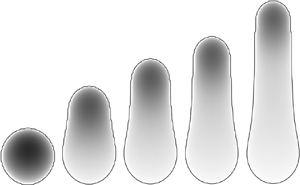
When the volume of fluid in a fracture exceeds $V_c$, the ascent of the fracture and contained fluid is self-sustaining. By this we mean that the ascent is due to buoyancy alone, and requires no additional forces such as a driving pressure (e.g. from a pressurised magma chamber or well bore). As the fracture ascends, the tail of the crack lengthens and thins, but the fracture head retains a volume sufficient to critically stress the medium ahead of it. Figure 1 shows numerical solutions, discussed below, which illustrate this.

Figure 1.

Numerical simulation of an ascending, finite batch of fluid. In this simulation, $1.95\ {\rm m}^3$ of fluid is injected over 130 s. Two views of the fracture are shown at each time. On the left-hand side is a view looking onto the fracture's face, shaded by aperture ($w$) with the tip-line in black. On the right-hand side is a grey cross-section showing the profile of the aperture along the centre of the crack. The latter has a horizontal exaggeration of $2\times 10^4$. (a) Analytical solution that defines the radius $a$. The plotted solution contains fluid volume $V$ and has a radius such that $K_I(z=-a)=0$. (b) Numerical simulation of the fracture ascent using PyFrac (table 1). Simulation times are shown below the respective fractures. The time-dependant analytical approximation of the fracture's cross-section is shown as dashed lines (Roper & Lister Reference Roper and Lister2007). The tail height $h$ from (3.10) is marked with a dot.

2.1.2. Ascent rate

Results cited above quantify the critical conditions for buoyant ascent, but not the speed of that ascent. The latter requires a consideration of the fluid flow within the fracture. In the tail of the fracture this can be usefully approximated as Poiseuille flow between parallel plates. At small Reynolds number, lubrication theory gives the mean flow speed $v$ and areal flux $Q_A$ as

(2.3a,b)\begin{equation} v=\frac{w^2}{12 \eta}\Delta\gamma,\quad Q_A=\frac{w^3}{12 \eta}\Delta\gamma, \end{equation}

where $w$ is the separation of the plates, $\eta$ is the dynamic viscosity and we have assumed that the gravity vector is parallel to the walls.

The ascent rate of a 2-D fracture with constant areal flux $Q_A$ is given by eliminating $w$ from (2.3a,b) to give (Lister & Kerr Reference Lister and Kerr1991)

(2.4)\begin{equation} v_Q=\left(\frac{Q_A^2\Delta\gamma}{12 \eta}\right)^{1/3}. \end{equation}

This result means that for $Q_A$ constant, the speed of the upper tip is controlled by viscous flow through a tail of constant width, which transports buoyant fluid upwards to the propagating head.

The ascent rate of a 2-D fracture with constant area $A$ is given by combining (2.3a,b) with a conservation of mass equation that relates the rate of change of aperture to the divergence of the vertical flux (Spence & Turcotte Reference Spence and Turcotte1990). On this basis, Spence & Turcotte (Reference Spence and Turcotte1990) obtained a solution in terms of the velocity of flow through a half-ellipse with a fixed area. As this lengthens vertically its aperture decreases, which hinders fluid flow and slows the ascent of the fracture tip. The rate at which the half-ellipse lengthens therefore progressively decreases with time. Differentiating with respect to time the equation (22) of Spence & Turcotte (Reference Spence and Turcotte1990), which defines the $z$ distance between the upper tip and the initial centre point of the fracture (the injection point), the fracture's tip velocity is

(2.5)\begin{equation} v_{A}(t)=\left(\frac{A^2 \Delta\gamma}{48 \eta}\right)^{1/3} t^{{-}2/3}. \end{equation}

The ascent rate of a 3-D fracture with a constant rate of volume injection was considered by Lister (Reference Lister1990b). His equation (2.14) provides an approximate 3-D scaling for fracture height, breadth and aperture at a given injection rate (see also Germanovich et al. Reference Germanovich, Garagash, Murdoch and Robinowitz2014). These scalings have been confirmed by Möri & Lecampion (Reference Möri and Lecampion2022) using 3-D numerical simulations computed with open-source codes (Salimzadeh et al. Reference Salimzadeh, Zimmerman and Khalili2020; Zia & Lecampion Reference Zia and Lecampion2020). Möri & Lecampion (Reference Möri and Lecampion2022) show that for a 3-D, constant injection-rate, ascending fracture, the shape of the tip-line depends on a dimensionless ratio that includes viscosity and fracture toughness. At early times, close to the injection point, viscous resistance limits tip-line propagation, resulting in a V-shaped tip line. Whereas later, sufficiently far from the injection point, fracture toughness limits tip-line propagation and the tip-line at either side of the fracture is vertical. In this study we are interested in how the ascent speed decays with time. In the case of buoyant ascent fed by a constant flux, the ascent speed in the viscosity-dominated regime is $v\propto t^{-1/6}$, whereas later, after transitioning to the toughness regime, the velocity is constant (Lister Reference Lister1990b; Germanovich et al. Reference Germanovich, Garagash, Murdoch and Robinowitz2014; Möri & Lecampion Reference Möri and Lecampion2022). These limiting regimes correspond with the asymptotic solutions for an aperture near the tip-line (Detournay Reference Detournay2004).

The ascent rate of a 3-D fracture containing a constant volume of fluid is not known.

2.2. Numerical methods

We run 3-D simulations of an ascending fluid batch with a constant volume using a hydro-fracture simulator. This 3-D simulator generates numerical solutions to the nonlinear governing equations. These solutions guide the development of our approximate analysis for constant-volume fractures. Comparison of our analytical and numerical solutions then enables us to determine the validity of simplifying assumptions and assess the accuracy of our analytical predictions.

We simulate the propagation of buoyancy-driven fractures using the open source code PyFrac (Version 1.0, https://pyfrac.epfl.ch). The methods and implementation of PyFrac are extensively documented in Zia & Lecampion (Reference Zia and Lecampion2020). The calculations we present use the code as described in that original work, and hence we only summarise the algorithm here to give a sense of its aptitude for solving hydro-fracture problems.

The hydro-fracture problem comprises three coupled physical aspects: fluid flow and pressure inside the fracture; deformation of the surrounding medium due to the fracture; and propagation of the fracture's tip-line into the unfractured medium. These aspects are independently modelled as low-Reynolds-number fluid flow, quasistatic linear elasticity and linear-elastic fracture mechanics. Although each is linear independently, their coupling results in a nonlinear equation system. The time-dependent solution to this system is the location of the tip-line, the fracture aperture, and the fluid pressure and velocity. The PyFrac solver limits the complexity of this problem by restricting solutions to be planar fractures. This simplification enables precomputation of the Green's functions required for the displacement discontinuity method using a fixed-grid mesh (Peirce Reference Peirce2016). The displacement discontinuity method links fluid pressure inside the fracture to the opening of its walls and to deformation of the surrounding medium. On the same mesh, the lubrication equation is discretised using the finite volume method at element centres. The gradients in fluid pressure determine the rate of flow between cells. Crucially, to avoid the requirement of ultrahigh mesh resolution near the fracture tip, PyFrac uses near-tip asymptotic solutions for propagating, fluid-filled fractures. These asymptotic solutions resolve the subgrid-scale dynamics, and hence are used to assess the propagation criterion and rate of tip-line motion. By comparison of numerical solutions to existing analytical solutions (Peirce Reference Peirce2015, Reference Peirce2016; Zia, Lecampion & Zhang Reference Zia, Lecampion and Zhang2018; Moukhtari, Lecampion & Zia Reference Moukhtari, Lecampion and Zia2020; Zia & Lecampion Reference Zia and Lecampion2020), it has been shown that PyFrac can accurately solve the coupled hydro-fracture growth problem.

For simulations in the present manuscript, the extent of the meshed domain in the horizontal direction is $2a$, where $a$ is the characteristic crack radius we define below. The vertical extent of the domain is sufficient to capture propagation of the fracture in the postinjection, buoyancy-driven regime without remeshing (a distance of $14a$). Along the horizontal direction we use a minimum grid size of 50 elements; the vertical grid is created such that the elements are square. We note that the meshed domain is only used to discretise the fracture itself. Displacements and stresses due to the fracture are described by Green's functions for an infinite space such that these hold anywhere in the body. The simulation presented here is initialised with a circular fracture of radius of $a/6$. The fracture aperture is a result of a uniform internal pressure such the critical stress intensity is attained around the tip-line ($K=K_c$). For this condition, an elapsed time since the start of injection is determined using an analytical solution, assuming the injection rate was constant (Detournay Reference Detournay2004). The remaining fluid volume is injected as part of the simulation, at a constant rate from a point source.

At each time step in the simulation, PyFrac returns the computed front velocity. This velocity fluctuates with a period of the order of the time step. The fluctuations, however, are small in amplitude and do not influence the general trend of the velocity. To remove them, we apply a moving average with a sampling width of 40.

The fluctuations arise from the numerical time-stepping scheme used to solve for the position of the moving fracture front, a scheme that is first-order accurate in time (Peirce & Detournay Reference Peirce and Detournay2008). To compute the advance of the front, the user of PyFrac can choose between three time-stepping schemes: implicit; explicit; and predictor corrector (Zia & Lecampion Reference Zia and Lecampion2019). We show a plot comparing filtered results for each of these schemes in Appendix B. Neither the scheme chosen nor the mesh size change the resulting trend of the front velocity. Following the example of Zia & Lecampion (Reference Zia and Lecampion2019), we have chosen the predictor–corrector front-advancing algorithm in this study.

2.3. Qualitative insights from numerical simulations of fracture ascent

Using the numerical method described above, we simulate the injection of a finite batch of buoyant fluid, closely following a case that was analysed by Salimzadeh et al. (Reference Salimzadeh, Zimmerman and Khalili2020). The parameter values for this simulation are provided in table 1.

Table 1.

Parameter values used for the simulation shown in figures 1 and 2. These correspond to simulation-case II from the main text of Salimzadeh et al. (Reference Salimzadeh, Zimmerman and Khalili2020).

In figure 1 we plot snapshots of the fracture's shape as it evolves through time. Time increases from left to right in the plot. Looking onto the fracture's face, approximately eight minutes after the injection has ceased (10 minutes), the fracture's tip-line is circular. Note the vertically asymmetric aperture of the cross-section at this time, which indicates that the fluid is starting to flow towards the upper tip of the fracture. After six hours the top of the fracture has grown upwards whilst the tip-line in the lower portion has not changed shape; when looking at the face at this stage, the tip-line on either side of the fracture tapers progressively towards the top. The form of the upper part of the tip-line is a semicircle and remains so throughout the rest of the simulation. As time increases the aperture in the lower parts of the fracture progressively thins. By six hours, the fracture has reached a characteristic shape; in cross-section, the lower half of the fracture (tail) is thin and V-shaped while the upper half (head) has formed the teardrop profile of a Weertman crack (Roper & Lister Reference Roper and Lister2007). Looking onto the face at 15 hours, the fracture's upper tip has continued to rise, resulting in a tip-line on either side of the fracture that is approximately vertical, where the tapering upwards is less evident. The cross-sectional aperture retains the typical structure predicted by 2-D analytical solutions, with a clearly defined teardrop-shaped head and tapered tail (Roper & Lister Reference Roper and Lister2007). This structure dominates at late times ($t>15$ h), noting the thinning of the tail as the length increases, whilst the head's shape remains roughly constant.

In figure 2(a) we plot the speed of the upper-most point on the fracture's tip-line as a function of time (log scale). We refer to this speed as the ascent rate because it is identical to the speed at which the head of the fracture rises through the medium. A dashed line shows $v \propto t^{-2/3}$; this scaling appears in the 2-D solution (2.5). At late times greater than six hours, the speed from the 3-D numerical solution approaches this $t^{-2/3}$ asymptote.

Figure 2.

Upper-tip ascent speed from the PyFrac simulation (solid line) and the predicted asymptotes and analytical approximations (broken lines). Times corresponding to steps in figure 1 are shown as asterisks. Parameter values are given in table 1. (a) Ascent rate versus time on a log–log plot. (b) Ascent rate versus height. Our prediction for the maximum ascent speed from (3.7) is shown as a horizontal dashed line. Also shown is the analytical approximation of the front speed produced using (3.10) and (3.11) (dash–dot line).

In figure 2(b) we plot the ascent rate as a function of the height of the fracture. Note the $y$-axis has a logarithmic scale and the times shown in figure 1 are plotted as asterisks. The plot shows two clear changes in front deceleration. The first occurs once the injection stops and the second occurs when the upper tip has propagated further than $2a$, a characteristic radius we examine later (Möri & Lecampion Reference Möri and Lecampion2021). We attribute the second transition in the front speed to a shift in the process driving tip-line growth: from injection-driven to buoyancy-driven fracturing. This transition occurs once the upper tip of the fracture has propagated a given distance. If this interpretation is correct then at later times the decay in ascent speed should be related to the fluid flowing upwards with an increasingly long and thin tail (2.5) (Spence & Turcotte Reference Spence and Turcotte1990). Such a thinning of the tail aperture can be seen in the snapshots of the ascending fracture in figure 1. In the following section we provide analytical expressions approximating: (i) the fracture's maximum lateral extent $a$ (figure 1); (ii) the maximal upwards propagation speed once injection has terminated (dashed line in figure 2b); and (iii) the deceleration of the ascending fracture with time (figure 2a).

3.1. Injection-driven front speed for constant injection rate

Previous studies of 2-D ascending finite batches of fluid placed the batch in the crust instantaneously and investigated how it subsequently evolves (Spence & Turcotte Reference Spence and Turcotte1990; Roper & Lister Reference Roper and Lister2007). Our 3-D approximate solution is informed by these 2-D solutions and also assumes that the finite fluid batch is fully emplaced before buoyant ascent occurs. In our 3-D numerical experiments, however, we have chosen to simulate injection of the fluid into the medium. We must therefore carefully choose a rate and duration of injection such that the fluid batch is emplaced before significant buoyant ascent has occurred, such that the approximation still holds. At early times, injection dominates the speed at which the fracture front advances; during this phase the fracture grows radially with a circular tip-line. In this section we consider how long injection of a given volume of fluid can last without overlapping the buoyant ascent phase. We therefore compare the front speed due to injection-driven growth and the front speed due to buoyant ascent.

The circular advance of the fracture tip driven by a constant injection rate in the absence of buoyancy is well understood (Detournay Reference Detournay2016). The growth of an injection-driven fracture can be separated into two regimes with distinct tip speeds: early times, when viscosity dominates the tip asymptote; and later times, where toughness dominates. Therefore, to compute the injection-driven front speed at a given time, we must determine which regime is dominant at that time. The transition time between viscous and toughness regimes occurs at

(3.1)\begin{equation} t_{mk}=\left(\frac{E'^{13} \eta'^5 Q_V^3}{K'^{18}}\right)^{1/2}, \end{equation}

where $K'=4(2/{\rm \pi} )^{1/2}K_c$, $E'=E/(1-\nu ^2)$ and $\eta '=12\eta$ and $Q_V$ is a constant volumetric fluid flux into the fracture (Detournay Reference Detournay2004).

We determine the injection-driven growth regime at the end of injection $t_I$ by comparing $t_I$ with $t_{mk}$. In the case that viscous forces dominate ($t< t_{mk}$), the speed of radial growth (${\rm d} r/{\rm d} t$) is

(3.2)\begin{equation} v_{rm}=b\frac{4}{9} \left(\frac{E' Q_V^{3}}{\eta' t^{5}}\right)^{1/9}, \end{equation}

where $b=0.6955$ (Detournay Reference Detournay2016). In the case that toughness controls growth ($t>t_{mk}$), Detournay (Reference Detournay2016) describe its radial speed as

(3.3)\begin{equation} v_{rk}= \frac{2}{5}\left(\frac{9}{2{\rm \pi}^2 } \frac{E'^2 Q_V^2 }{K'^2 t^3}\right)^{1/5}. \end{equation}

Note, the volume injected at time $t$ is $Q_V t$. We use the relevant estimate of front speed at $t=t_I$ to make a comparison with the buoyant ascent speed. To this end, we next derive an approximate upper bound on the rate of buoyant ascent if the fracture is circular and filled with volume $V$.

3.2. Early-time ascent rate

Here we aim to approximate the ascent rate of a buoyancy-driven fracture after injection ceases, when the front speed becomes dominantly driven by buoyancy. This moment does not occur precisely at the end of injection; some growth beyond that time is driven by the release of elastic energy stored during the injection phase, which drives a radial motion of the tip line (Möri & Lecampion Reference Möri and Lecampion2021). This energy is expended rapidly, after which buoyancy dominates the front speed. Our first calculation is an estimate of the speed of ascent at this point. We assume that a volume $V$ of fluid has been injected and resulted in a penny-shaped crack. The crack has extended radially to a size such that the deepest segment of the tip line, the bottom tip, has ceased its radial advance. The walls of the crack are subject to a downwards stress gradient of magnitude $\Delta \gamma$ that drives fluid upward. As this gradient becomes dominant post injection, the fracture above the bottom tip begins to drain fluid and pinch closed. Injection of a volume $V$ leads to a penny-shaped crack with mean internal pressure given by

(3.4)\begin{equation} p_0=\frac{3\mu}{8(1-\nu)}\frac{V}{a^3}, \end{equation}

where $a$ is the radius of the tip-line around the injection point (Tada et al. Reference Tada, Paris and Irwin2000). The mode-I stress intensity at the circular tip line arises from a combination of $p_0$ and the linear stress gradient (Tada et al. Reference Tada, Paris and Irwin2000),

(3.5)\begin{equation} K_I(\theta) = \frac{2}{\rm \pi}\sqrt{{\rm \pi} a}\left(p_0 + \frac{2}{3}\Delta\gamma a \cos(\theta)\right), \end{equation}

where $\theta$ is the angle in the $y$–$z$ plane away from vertical. If $z$ is the upwards distance from the injection point, eliminating the mean pressure from (3.4) and (3.5) and requiring that at the basal tip $K_I(z=-a)=0$ gives the radius of the crack as

(3.6)\begin{equation} a=\left(\frac{9 \mu }{16 (1-\nu) }\frac{V}{\Delta\gamma}\right)^{1/4}. \end{equation}

The mean aperture of this crack is simply given by $w = V/{\rm \pi} a^2$. Using this in (2.3a,b) to compute the characteristic fluid ascent speed $v$, then combining the result with (3.6) to eliminate $a$ we obtain

(3.7)\begin{equation} \tilde{v}_{V}=\frac{4(1-\nu)}{27{\rm \pi}^2\mu} \frac{\Delta\gamma^2 V}{\eta}\quad \text{for }V>V_c. \end{equation}

Here we have assumed that the fluid ascent speed $v$ is equal to the speed of the upper tip line $\tilde {v}_V$. The tilde indicates that this is an early-time solution and the subscript $V$ indicates that this is a fixed-volume, 3-D fracture. This speed is plotted as a horizontal dashed line in figure 2(b).

3.3. Radial growth versus buoyant ascent

Equation (3.7) is the speed of the upper tip while the crack is still penny-shaped, just after the phase of radial growth driven by the injection. As the upper tip propagates, driven by buoyancy of the fluid, the crack elongates vertically. The stress gradient drives fluid within the crack upwards such that part of the total fluid volume $V$ resides in the head of the crack, while the remainder forms a slowly thinning layer in the long tail (figure 1). Thus, (3.7), which describes the instant when the entire fluid volume is in the head and the lower tip reaches its maximum depth, gives an approximate upper bound on the buoyancy-driven ascent speed. Before proceeding to derive a late-time solution for the ascent speed, we use the result above to compute a maximum duration of injection $t_V$. If injection continues far beyond this, the assumption of rapid fluid emplacement in the 3-D analytical solution we introduce below will no longer hold.

The time at which buoyant ascent becomes dominant in determining the front speed can be approximated as the moment when the injection-driven front speed is equal to the buoyant ascent speed. We have approximated the latter with (3.7). We denote this crossover time $t_V$ and obtain values for each of the two injection regimes. For a viscosity-dominated circular crack, the speeds predicted by (3.7) and (3.2) are equal at

(3.8)\begin{equation} t_{Vm}=\left[ \left(\frac{b {\rm \pi}^2}{8 \Delta\gamma^2}\right)^9 \frac{E'^{10} \eta'^8}{ Q_V^6 } \right]^{1/14}. \end{equation}

For a toughness-dominated circular crack the front speeds described by (3.7) and (3.3) are equivalent at

(3.9)\begin{equation} t_{Vk}=\frac{9}{4}\left(\frac{3 {\rm \pi}^9}{5^5}\frac{ \eta^5 E'^7 }{ \Delta\gamma^{10} K_c^2 Q_V^3 }\right)^{1/8}. \end{equation}

We now show how to use these equations on an example case, the simulation in figure 1 (table 1). We first determine which regime the front was in at the end of injection (3.1). Because the duration of injection $t_I$ was 130 s and $t_{mk}$ is 400 s, we conclude that this was in a viscosity-dominated regime when injection ceased.

We then determine the time at which the injection- and buoyancy-driven front speeds would be equal. Equation (3.8) provides the time when (3.7) and (3.2) are equal, at $t_V = 720$ s. The injection time $t_I$ is much shorter than this, and hence the fracture is approximately circular when the injection stops. Figure 1 confirms this; the fracture is still circular around eight minutes after the injection stopped at $t_I$. If $t_I$ is below or of the same order of magnitude as $t_{V}$, the fracture will remain close to circular at the end of injection.

Having clarified the requirements to emplace the batch of fluid such that our assumptions hold, we next focus on the late time solution, long after injection has ended.

3.4. Finite propagation with deceleration

We now consider the vertical advance of the fracture over finite time. We define $h$ as the vertical distance between the fracture's upper tip and the initial centre of the crack (the injection point). Recalling that figure 2(a) shows the ascent rate of the 3-D simulation asymptotically scales with time as predicted by (2.5), this motivates us to approximate the 3-D ascent speed using this 2-D solution. To retrieve $h(t)$ and $v(t)$ for our 3-D fracture, we modify the similarity solution obtained by Spence & Turcotte (Reference Spence and Turcotte1990, (22)) for a 2-D fracture with constant area. Replacing that area $A$ with the initial cross-sectional area of the 3-D crack $2aw$ gives

(3.10)\begin{equation} h=\left(\frac{9 \left(2 a w\right)^2 \Delta\gamma t}{16 \eta}\right)^{1/3}. \end{equation}

Substituting (3.6) and $w = V/{\rm \pi} a^2$ into (3.10) and defining the speed $v_V(t) \equiv \textrm {d} h/\textrm {d} t$, we obtain

(3.11)\begin{equation} v_V(t)={\left(\frac{\left(1-\nu\right)}{9^2 {\rm \pi}^4 \mu } \frac{\Delta\gamma^3 V^3}{\eta^2 }\right)}^{1/6} t^{{-}2/3}. \end{equation}

This approximate solution might be expected to hold at later times, when buoyancy has driven the fracture to propagate away from the injection point, establishing distinct tail and head regions of the fracture.

Figure 2(b) shows the predicted initial and late-time speeds from (3.7) and (3.11), respectively. The figure also shows a numerical solution of a 3-D crack for the same parameter values. The ascent rate predicted by (3.11) at $h=2a$ is greater than the numerical result at the same position; at this point, the early-time approximation (3.7) fits better. At $h/2a = 3/2$, the two approximations are equal $\tilde {v}_V=v_V(t)$. As the fracture ascends beyond this height, the full numerical solution and the late-time solution converge. This convergence was also obtained in 2-D numerical solutions by Roper & Lister (Reference Roper and Lister2007, figure 9).

3.5. Comparison between the numerical results and analytical predictions

Using the initial cross-sectional area $2aw$ noted above, we plot as dashed lines in figure 1 the cross-section predicted by the 2-D similarity solutions of Roper & Lister (Reference Roper and Lister2007, § 6). See our Appendix A for the equations used in this calculation. The height of the tail in these cross-sections is given by (3.10). Focusing attention on the solutions at an elapsed time of 30 hours, the analytical solution provides a good fit to the width of the tail from the numerical solution. Furthermore, the simulated fracture's head length and shape are approximately that of the Weertman solution. The notable discrepancy is that the analytical solution predicts a greater propagation distance than produced by the simulation. This discrepancy is also evident in the comparison of fracture ascent speeds of figure 2(b) where, initially, the analytical prediction is for faster propagation, but as the simulation progresses and the fracture lengthens, the numerical and analytical speeds converge. Next we discuss the assumptions made in the derivation of (3.11) to explain why the numerical and analytical ascent rates and heights differ.

We begin with a reminder of three insights from 2-D results by Roper & Lister (Reference Roper and Lister2007) that also apply here. Firstly, as long as the cross-sectional area of the initial 2-D crack is above the critical head area given by (2.1), the fracture is predicted to ascend indefinitely, with a monotonically decreasing propagation rate. Secondly, in the 2-D, constant-area theory, elastic forces dominate in the head region, resulting in a head shape that remains constant over time and is described by the static Weertman solution (Weertman Reference Weertman1971; Rubin Reference Rubin1995). Thirdly, Roper & Lister (Reference Roper and Lister2007) show that the area of the head should be removed from the total area when computing the dynamics of the tail (e.g. (3.10)) and, in particular, in estimating the velocity and height of the fracture.

Keeping these insights in mind, we next evaluate assumptions of the 2-D, constant-area approximate solution in comparison with observations from our 3-D simulation from figure 1. In the 2-D solution, the areal extent of the head is constant during ascent, whereas in the 3-D simulation, the effective head volume decreases due to a tapering head breadth. Defining the head volume as open areas of the fracture from the upper tip down to a distance of $2c_h$ below this, we find that in simulations, the 3-D head volume decreases until it stabilises at a value around that of $V_c$. This reduction of the head volume is qualitatively shown by the lateral tip-lines in figure 1 that slightly converge upwards over time. Because of this feature, we have neglected to approximate the head volume, placing the entire cross-sectional area of the initial penny-shaped crack into the tail solution. Our analytical result is therefore based on an overestimate of the tail volume, and hence it should predict a faster ascent rate than the numerical simulation. This explains why initially, the predicted velocities are faster. Moreover, in the 2-D solution (3.10), the cross-sectional area of the fluid (tail plus head) is constant. This contrasts with observations in the simulation shown in figure 1 where along the centreline, the fracture's cross-sectional area increases by 36 % from the earliest (10 minutes) to the latest (60 hours) snapshots. This out-of-plane fluid flow is, by definition, not captured by the 2-D solution. Thickening of the cross-section in the 3-D simulation suggests that the ascent rate for a 3-D fracture will be faster than its 2-D analogue at later times, such that our solution will underestimate the ascent rate.

4.1. Testing across length scales by comparison to numerical solutions

We now test our analytical approximations against numerical solutions across a wider range of physical parameters. Here, each parameter set represents a different physical context: analogue experiments with oil-filled cracks in gelatine; an industrial setting where water is injected into a shale sequence; and the ascent of a basaltic dyke through the crust (table 2). We compare our analytical prediction from (3.11) against rates obtained from PyFrac calculations using the three parametric combinations listed in table 2, each of which is simulated for three different injection volumes to give nine total models. Results are shown in figure 3, in comparison with analytically predicted rates. The comparison shows that $v_V(t)$ from (3.11) provides a reasonable match to the numerical results across all parameter sets considered. The analytical results predict the PyFrac velocities within a factor of two. The ratio of numerical to analytical ascent speed is approximately constant for a given simulation. In figure 4, we compare our analysis (3.10) with numerical results in terms of the time-dependent height of the upper tip above the injection point. As in the previous figures, we find the fracture must ascend by a length of more than $2a$ (box shown is $3a$) before buoyancy becomes the dominant driver of propagation. After that time, the results show the predicted and simulated heights are comparable. These comparisons show that our analytical approximations capture the leading-order fracture ascent speed across a broad parameter space. We further note that our analytical results for the extent and ascent speed provide a reliable means to forecast the required PyFrac domain size and simulation duration for a given set of parameters, such that the numerical model converges and completes the intended simulation.

Figure 3.

Numerical versus analytical (3.11) speed estimates at times $t$ since injection. Plotted are nine simulations performed using the code of Zia & Lecampion (Reference Zia and Lecampion2020) and summarised in table 2. These comprise three parametric cases, each with three different injection volumes and rates. The plots stop at the point when the simulated fracture reached the edge of the meshed domain or Pyfrac terminated the simulation.

Figure 4.

Numerical versus analytical (3.10) height estimates at times $t$ since injection. Height here is defined as the distance from the injection point to the upper tip. This plot uses the same numerical solutions as in figure 3.

Table 2.

Properties used to numerically simulate fracture ascent for different physical processes. The injection rate for such cracks is set to $t_I=(V \, \tilde {v}_V)/a$, such that the injection is complete before the fracture ascends past $h=2a$. Note this results in $\tilde {v}_{V}/v_r$ to $\sim$2 for all results. Here $t_I/t_{mk}$ for $V_I/V_c=2$, 10 and 100 are $1.7\times 10^{4}$, 45 and $2\times 10^{-2}$, respectively; as such these span both viscous and toughness dominated radial growth regimes at the point at which the injection stops.

4.2. Comparison to analogue oil injection gelatine experiments

The gelatine experiments of Heimpel & Olson (Reference Heimpel and Olson1994) and Smittarello (Reference Smittarello2019) show that crack ascent rates are related to the injected volume. Our analysis can be used to understand what determines the speed of fractures in such experiments. Taisne & Tait (Reference Taisne and Tait2009) noted that many fluids typically injected, such as air and some oils, are non-wetting when in contact with gelatine solids. When these flow through fractures in gelatine, the lubrication approximation breaks down; all fluid can be expelled from between the walls. Both effective closure of the fracture's tail and near-constant ascent rates are indications that non-wetting processes are active. As such, Taisne & Tait (Reference Taisne and Tait2009) suggest that experiments that use non-wetting fluids may not be a good analogue for natural settings.

Silicon oils are wetting with respect to the gelatine. In figure 5 we plot the speed of silicon oils hydro-fracturing upwards through gelatine solids from Smittarello (Reference Smittarello2019). The material properties are given in table 3 and the experimental set-up is described in Smittarello et al. (Reference Smittarello, Pinel, Maccaferri, Furst, Rivalta and Cayol2021). These experiments have well-constrained injection volumes and elastic parameters, and therefore provide a suitable basis for comparison with our equations. Note, the rate of injection was not constant in these experiments.

Figure 5.

Upper tip height from analogue experiments where silicon oil is injected into gelatine solids. Parameter values are given in table 3. (a) Height versus time, showing that at late times, curves approach the $t^{1/3}$ asymptote (dash–dot). The triangles denote the end of injection ($t_I$). (b) The height from the experiments is plotted against the predicted speed using (3.11), where the time is that elapsed since the start of the injection. The predicted heights have been translated such that they are equal to the observed height at $t=2 t_I$ (squares).

Table 3.

Properties of the analogue gelatine experiments of Smittarello (Reference Smittarello2019). Experiment reference numbers are shown in the first row. Note that the injection rates were not recorded. Note here the reported values of $K_c$ are estimated using an empirical formula based on the shear modulus, reported in § 3.1 of Davis et al. (Reference Davis, Rivalta and Dahm2020).

In these experiments, a tank is filled with liquid gelatine that is allowed to solidify, then a buoyant fluid is injected at the base of the tank to form a fluid-filled fracture. This fracture ascends through the gelatine and its position is measured at regular time intervals. Figure 5(a) shows that after the postinjection transient ends, the length of the experimental fractures broadly follow a $t^{1/3}$ trend, as predicted by (3.10). Figure 5(b) shows the predicted late-time fracture lengths are around double that observed. Note that the predicted heights have been translated such that the fracture lengths are equal to the observed lengths following injection (at $t=2 t_I$). The results follow the $t^{1/3}$ trend at late times, but the magnitude of the prediction is too high. The critical volume $V_c$ required for ascent in table 3 is close to the injected fluid volume $V_I$, and our prediction assumes the entire fluid volume is in the fracture tail, as discussed earlier. When $V_I\approx V_c$, the majority of fluid is actually contained in the fracture head during ascent. Less fluid in the tail means slower draining out of the tail; this may explain why we predict ascent rates that are faster than observed. Moreover, model predictions neglect the presence of tank walls and free surface (Smittarello Reference Smittarello2019). Experiment 1967 shows a deceleration as it approaches the surface where a load is placed on the gelatine to deflect the crack from vertical.