

1. Introduction
Canadian English is complicated. Claims of geographical homogeneity are long-standing, which has contributed to a public perception of Canadian English being relatively homogeneous. Statements of homogeneity, however, are often subsequently hedged with recognition of different accents in the Englishes in the Atlantic region—Newfoundland, New Brunswick, Nova Scotia and Prince Edward Island—and Quebec. This leaves the assumption in place that geographical homogeneity in the English variety holds from the Western coast to Ontario: “That a single urban, middle-class variety of Canadian English (CanE) is spoken from the eastern border of Ontario to the western coast of Vancouver Island in British Columbia is a claim asserted in work ranging from foundational Canadian dialectology to state-of-the-art dialect geography” (Denis & D’Arcy, Reference Denis and D’Arcy2019:223). These broad-strokes claims also must pause and acknowledge that the speech patterns of those in the northern regions—Nunavut, Yukon, and Northwest Territories—and individuals in the northern areas of comparatively well-studied provinces (Ontario, Manitoba, Saskatchewan, Alberta, and British Columbia) are understudied. Furthermore, geographical areas and regions even within the boundaries of British Columbia vary widely in terms of their population size and composition, adding to the complexity of understanding what it means for Canadian English to be geographically homogeneous.
The goal of the current work is to further interrogate the degree of synchronic regional accent homogeneity or heterogeneity in British Columbian English and by extension Canadian Englishes. This project builds on older and contemporary work that, indeed, finds accent variation in Canadian English. For example, regional variation reported in older work, such as Polson (Reference Polson1969) on English spoken in Northern BC, Yukon, and Northwest Territories, and more recent work on Northern Ontario English vowel variation (Smith, Reference Smith2018), English spoken in Victoria across apparent time (Roeder, Onosson & D’Arcy, Reference Roeder, Onosson and D’Arcy2018), and English spoken in Canada (Boberg, Reference Boberg2008, Reference Boberg2010) all call into question the veracity of claims about accent uniformity in Canada. Boberg (Reference Boberg2010) mentions the Canadian North as being a region with a variety of English separate from other regions (see also Polson, Reference Polson1969), and that due to historical settlement patterns, there are “subtle differences between the types of English that can be heard in Ottawa or Toronto and in Calgary or Vancouver; these differences are not necessarily detectable only to the ears of a trained phonetician. This presents a challenge, if only a minor challenge, to the conventional view that Canadian English is geographically homogeneous over the vast territory extending from Vancouver to Ottawa” (Boberg, Reference Boberg2008:150).
Part of the issue at hand is what counts as minor variation? When does the homogeneous label get applied? As noted, several scholars observe differences across regions but still embrace the homogeneity myth of Canadian English. For example, in Smith’s study on vowels in Northern Ontario he observes: “despite some regional differences, the vowel systems of Kirkland Lake and Temiskaming Shores are essentially similar to those of Toronto and Thunder Bay, and that this underlying stability corroborates the longstanding claim of homogeneity of English across Canada” (Smith, Reference Smith2018:iii; see also Roeder et al., Reference Roeder, Onosson and D’Arcy2018).
We suggest that the claims of relative homogeneity should be questioned, given that there has been evidence in the literature of both regional and socio-cultural variation in English spoken in Canada since the 1950s (e.g. Gregg, Reference Gregg1957; Pringle & Padolsky, Reference Pringle and Padolsky1983; De Wolf, Reference De Wolf1990; Woods, Reference Woods and Cheshire1991; Boberg, Reference Boberg2008; Onosson, Reference Onosson2010; Thorburn, Reference Thorburn2014; Mellesmoen, Reference Mellesmoen2016, Reference Mellesmoen2018; Onosson, Rosen & Li, Reference Onosson, Rosen and Li2019). This variation has been documented in sound structure (e.g. Chambers & Hardwick, Reference Chambers and Hardwick1986; Hall, Reference Hall2000; Boberg, Reference Boberg2008, Reference Boberg2010; Rosen & Skriver, Reference Rosen and Skriver2015; Roeder et al., Reference Roeder, Onosson and D’Arcy2018; Onosson, Reference Onosson2022; Denis, Elango, Kamal, Prashar & Velasco, Reference Denis, Vidhya Elango, Prashar and Velasco2023), lexically (e.g. Bailey, Reference Bailey1991; Dollinger, Reference Dollinger2019), and grammatically (e.g. De Wolf, Reference De Wolf1990; Denis, Reference Denis2020). Furthermore, the relationship between historical patterns of settler colonialism and its relationship to claims of geographical homogeneity have been investigated (e.g. Denis & D’Arcy, Reference Denis and D’Arcy2019, Reference Denis and D’Arcy2022; Denis, Reference Denis2020). Despite this evidence—and even with it (e.g. Chambers & Hardwick, Reference Chambers and Hardwick1986)—the influential proposal of homogeneity in Canadian English has been hard to shake (but see e.g. Pringle, Reference Pringle, Allen and Linn1986; Lilles, Reference Lilles2000; Hoffman & Walker, Reference Hoffman and Walker2010; Dollinger, Reference Dollinger2019).
Investigations of Canadian English often contend with limited geographical sampling, in addition to confronting narrow population sampling within a region, which may further complicate our understanding of variation in the English spoken in Canada. Sociolinguistic and dialectological work within Canada often acknowledges that the inquiry of Canadian English is limited to urban centers, speakers with an Anglophone heritage, or speakers labeled as “standard.” This is demonstrated by the dominance of the term “Canadian English” in academic and public contexts to refer to the concept of a largely homogeneous variety. By defaulting to the label “Canadian English” and so investigating “Canadian English” as a variety as a whole, which is a common trend regardless of the location of the sample population, the research implicitly assumes homogeneity from the outset. It also contributes further to the perception of homogeneity in the literature and for the public. Pringle (Reference Pringle, Allen and Linn1986:232) asserts: “[i]t is not just that urban Canadian English is not absolutely uniform […] but […] once you get out of the cities, Canadian English proves to be enormously varied.” In other words, describing “Canadian English” as homogeneous is problematic even with the previous caveats given what we know from previous work, and also as a result of the fact that the participant samples typically described and used in these studies are not representative of a large number of English speakers in the current (and likely the past) population. There is a range of historical factors and socio-cultural contexts in many areas of Canada which mean that a young, urban, middle-class, white, Anglophone heritage sample is not representative of the populations in many areas of Canada. Previous work has investigated the relationship between historical patterns of settler colonialism and its relationship to claims of geographical homogeneity and also Canadian English as a normative variety (e.g. Denis & D’Arcy, Reference Denis and D’Arcy2019, Reference Denis and D’Arcy2022; Denis, Reference Denis2020). It is clear that our empirical foundations are lacking, particularly for regions and populations that have been marginalized in the past.
The current investigation is a first step towards understanding synchronic regional variation at the community level in British Columbia. Using a more diverse speaker sample, we provide evidence for regionally defined variation within British Columbia for a set of phonological features that have been reported relatively extensively in varieties of English spoken in Western Canada, the Pacific Northwest, or across all of Canada. These phonological features are described in more detail below, but briefly, they are variables that have featured in linguistic investigations of the English spoken in Canada and in the Pacific Northwest. As such, they are well suited for assessing the extent of heterogeneity or homogeneity of Canadian Englishes. In this paper, we do not consider known socio-cultural factors, such as race and ethnicity, which have been shown to condition variation in perception and production in Canada (see e.g. Hoffman & Walker, Reference Hoffman and Walker2010; Babel & Russell, Reference Babel and Russell2015; Wong & Babel, Reference Wong and Babel2017; Presnyakova, Umbal, & Pappas, Reference Presnyakova, Umbal and Pappas2018; Nagy, Reference Nagy, Montrul and Polinsky2021; Denis et al., Reference Denis, Vidhya Elango, Prashar and Velasco2023). Our focus is explicitly on synchronic regional differences in the Englishes spoken in these speech communities and not on socially structured variation that occurs within and across these regions of British Columbia. We, therefore, do not explicitly provide an analysis of how the social demographics stratify speech patterns within the community. Simply, we are asking does English sound different in these regions of the province? While the current focus is on two regions of British Columbia (the Lower Mainland and the Okanagan), we continue to collect data from speakers across the province to broaden our reach and paint a more accurate and empirically rich picture of British Columbia Englishes.
1.1. Regional variation in Canada and British Columbia
The variationist tradition in Canada has generated a large body of literature, and we narrow our overview in this section to research that homes in on regional variation in sound structure and includes British Columbia or “the West.”
Boberg (Reference Boberg2008) suggests that there are six regional divisions of “Standard” English in Canada based on a sample of young, university-educated participants, who are second-generation to the specific Canadian regions they represent. He suggests that the West is a major division, which includes the prairie provinces (Alberta, Saskatchewan, and Manitoba, along with northwest Ontario) and BC, but that BC is also differentiated from the prairie provinces for some of the phonological features investigated, such as foot lowering.Footnote 1 While some evidence suggests that BC varieties differ from other varieties of Canadian English, the patterns described in BC varieties do not seem to be wholly categorizable as innovative or conservative compared to Canada-wide patterns (Roeder et al., Reference Roeder, Onosson and D’Arcy2018). In cases where regional variation has been discussed, BC has generally been included in a western region, which also often includes prairie provinces (e.g. Warkentyne, Reference Warkentyne1971; Labov, Ash & Boberg, Reference Labov, Ash and Boberg2006).
Much of the work that discusses “BC English” has either explicitly collected data from speakers in Vancouver or does not indicate where speakers are from. This means that speaker samples from Vancouver and its surrounding metropolitan area have most often been used to represent the English spoken in the province in comparisons against other urban centers in Canada such as Ottawa (e.g. De Wolf, Reference De Wolf1983, Reference De Wolf1990), Toronto (e.g. Chambers & Hardwick, Reference Chambers and Hardwick1986; Hall, Reference Hall2000), Montreal (e.g. Hung, Davison & Chambers, Reference Hung, Davison, Chambers and Clarke1993), or to areas of the neighboring Pacific Northwest region in the United States (e.g. Washington State, Dollinger, Reference Dollinger2012; Sadlier-Brown, Reference Sadlier-Brown2012; Swan, Reference Swan2020). Therefore, most of what is known about English spoken in BC to date describes speakers from a relatively small group: largely educated, white, of Anglo ancestry, and urban.
The oldest work on BC Englishes, while valuable, has these pitfalls. Going back over the past seven decades, there have been projects that have focused on English as it is spoken in BC (and this scholarship informs the current work), which were lacking in some respect, either due to the small sample size, the exclusivity of the sample population itself, or utilizing phonetic measurements that do not sufficiently capture the ways in which listeners experience the phonetic signal. Robert Gregg and a number of his students undertook projects, such as the “Linguistic Survey of BC English,” which produced Polson (Reference Polson1969), and “The Survey of Vancouver English” (Gregg, Reference Gregg1992). These projects described select phonological patterns in BC English, such as the presence of Canadian Raising of price and mouth, provided evidence in the form of phonetic transcriptions and comments for other phonological patterns, such as pre-velar raising of dress in Vancouver (Gregg, Reference Gregg1957), in addition to documenting regional pronunciation differences in select words between Vancouver Island, the Okanagan, and the Lower Mainland (Stevenson, Reference Stevenson1976), and pronunciation variation indexed to speech style in Vancouver (Richards, Reference Richards1988).
More recent work provides further evidence of regional variation in the English spoken in BC. Chambers & Hardwick (Reference Chambers and Hardwick1986) and Hung et al. (Reference Hung, Davison, Chambers and Clarke1993) describe differences in the Englishes spoken in Vancouver and Victoria. While Chambers & Hardwick suggest that Canadian Raising of mouth may be waning in Vancouver, Hung and colleagues find that Canadian Raising of mouth is not declining in Victoria. The mouth vowel in Vancouver is also subject to more rounding than in Victoria (Chambers & Hardwick, Reference Chambers and Hardwick1986; Hung et al., Reference Hung, Davison, Chambers and Clarke1993). Pappas & Jeffrey (Reference Pappas and Jeffrey2013) find that Victoria speakers produce more fronted onglides in mouth in Canadian Raising contexts compared to those from Vancouver.
Pappas & Jeffrey (Reference Pappas and Jeffrey2013) studied the Canadian Shift, which involves the lowering and/or retraction of the front lax vowels, among other changes (Clarke, Elms & Youssef, Reference Clarke, Elms and Youssef1995). They found active evidence of trap retraction in Vancouver and Victoria, continuing the patterns found in Esling & Warkentyne (Reference Esling, Warkentyne and Clarke1993). Pappas & Jeffrey also found retraction of dress. More recently, Presnyakova, Umbal & Pappas (Reference Presnyakova, Umbal and Pappas2018) found differences in the realization of the Canadian Vowel Shift in Vancouver that was conditioned by the heritage of the speaker. They compare speakers with British, Cantonese, South Asian, and Filipinx heritage, and found that Cantonese heritage English speakers retract kit more than the other groups and Filipinx heritage English speakers lower trap more than the other groups. Roeder et al. (Reference Roeder, Onosson and D’Arcy2018) also find that speakers of English in Victoria participate in the Canadian Shift, where it is a more recent development than elsewhere in Canada.
Roeder et al. (Reference Roeder, Onosson and D’Arcy2018) also examine back vowel fronting, retraction of start, the realization of the voiced palatal glide (yod), and pre-velar (bag) and pre-nasal (ban) raising of trap in order to assess the extent to which English spoken in Victoria aligned with descriptions of the Western dialect region of Canada. Among these variables there is evidence that Victoria English does “mostly” pattern with the varieties in the western region. In other words, there are some regionally specific patterns. The most relevant findings to our current investigation are that mid-point ban and bag are found to be raised and fronted to a similar degree and that there is no evidence that change in apparent time for these two variables has occurred.
1.2. The current investigation
This previous work points to regional variation as differences in magnitudes of a phonological pattern rather than presence or absence of a pattern. Given this, we limit our study to phonological patterns that are likely present in BC, as their existence is supported by previous work.Footnote 2 We consider magnitude differences as evidence of regionally specific patterns and, so, indications of heterogeneity. In other words, the goal of this investigation is not to confirm whether English speakers in different regions of BC participate in these phonological patterns, but to use these known phonological patterns as a lens into the existence of regional variation. Our analyses thus provide a qualitative affirmation of the existence of these phonological patterns, and we focus our analysis and discussion on the identification of differences by geographical region. Limited by the data collected thus far, as described below, our analysis focusses on the speech patterns from speakers in the Greater Vancouver Area and the Okanagan regions. Region in British Columbia, however, can be tightly coupled with ethnicity. The percentage of individuals in the Greater Vancouver Area who identify as visible minorities is 48.9% and as Indigenous or First Nations (labeled “Aboriginal” in the census) is 2.5%, while all Okanagan census districts have fewer than 10% of individuals identifying as visible minorities and 6% identifying as Indigenous or First Nations (Statistics Canada, 2016b, 2016c). Thus, we can assume our Greater Vancouver Area participants are both more diverse and exposed to more ethnic diversity. Participants were not asked about ethnicity during data collection. Importantly, we consider this a socially responsible decision, as it was based on public feedback, which highlighted concerns about questions around social identity and ethnicity. These questions were not viewed as relevant by community members. We reiterate, however, that our focus is on regional Englishes in British Columbia, and while there may be differences in ethnicity across regions, this ultimately translates into differences in the varieties spoken “on the ground” in these regions, thus inextricably crossing region and ethnicity in ways that we do not disentangle in the current investigation. Our analysis focuses on four phonological variables, all of which are either suggested to be features of the Canadian West or Canada as a whole: (i) Canadian Raising of price; and the behavior of the three front lax vowels (ii) kit, (iii) dress, and (iv) trap in pre-velar environments.
Canadian Raising was notably described as a feature of English in Canada by Joos (Reference Joos1942) and Chambers (Reference Chambers1973), but had been mentioned in even earlier descriptions of English in Canada (Emeneau, Reference Emeneau1935) and in the United States (Primer, Reference Primer1890). In Canadian varieties of English, Canadian Raising is a phonological pattern, whereby the nucleus of the price and mouth diphthongs are raised and/or fronted before voiceless consonants such that the vowels in the words like site and side are pronounced distinctly from each other. Canadian Raising has been found to be a feature of English spoken in most areas of Canada (Labov et al., Reference Labov, Ash and Boberg2006; Boberg, Reference Boberg2008, Reference Boberg2010) and has been consistently reported as a feature of English spoken in BC (e.g. Gregg, Reference Gregg1957; Chambers & Hardwick, Reference Chambers and Hardwick1986; Hung et al., Reference Hung, Davison, Chambers and Clarke1993; Rosenfelder, Reference Rosenfelder2007; Pappas & Jeffrey, Reference Pappas and Jeffrey2013).
The other three phonological variables involve the patterns of three front lax vowels kit, dress, and trap before voiced velars. These phonological patterns have been termed pre-velar raising, as the vowel before voiced velars is more raised, fronted, and/or diphthongized than in other environments, minimizing the acoustic-auditory difference between leg, lag, and lake. It has been suggested that pre-velar raising of trap occurs in English as it is spoken across most of Canada (Boberg, Reference Boberg2008; Labov et al., Reference Labov, Ash and Boberg2006) and has been attested in English spoken in BC for decades (Gregg, Reference Gregg1957; Mellesmoen, Reference Mellesmoen2018; Roeder et al., Reference Roeder, Onosson and D’Arcy2018; Swan, Reference Swan2020). Pre-velar raising of dress has a much smaller geographical distribution and has mainly been reported in the Pacific Northwest (e.g. Reed, Reference Reed1952; Wassink, Squizzero, Scanlon, Schirra & Conn, Reference Wassink, Robert Squizzero, Schirra and Conn2009; Wassink, Reference Wassink2015; Swan, Reference Swan2020) and eastern seaboard (Kurath & McDavid Jr., Reference Kurath and McDavid1961; Wells, Reference Wells1982) of the US and in Canada (e.g. Boberg, Reference Boberg2008; Mellesmoen, Reference Mellesmoen2018; Swan, Reference Swan2020). Finally, pre-velar raising of kit has so far not been reported in Canada, though it is documented in velar nasal environments in San Francisco (Cardoso, Hall-Lew, Kementchedjhieva & Purse, Reference Cardoso, Hall-Lew, Kementchedjhieva and Purse2016). However, there are reasons to suggest that this pattern may also occur, including anecdotal reports of speakers producing pre-nasal kit with a raised, fronted, and/or tensed vowel and the fact that the front lax vowel system tends to participate in uniform phonological patterns (e.g. the Canadian Shift; Clarke et al., Reference Clarke, Elms and Youssef1995). Thus, given pre-velar raising in BC involves the other two front lax vowels, the propensity for system-wide phonological pattern, and anecdotal reports, we include an analysis of pre-velar raising of kit.
We are, therefore, providing a quantitative analysis of two phonological variables that have been reported across Canada (Canadian Raising and pre-velar raising of trap), one variable that is found in the Pacific Northwest (pre-velar raising of dress), and one variable that has not been studied but is likely to occur in the English spoken in BC (pre-velar raising of kit), to investigate regional variation in English spoken in different areas of BC.
2. Methods
2.1. Data collection
Data were collected through DRAWL (http://blogs.ubc.ca/drawl/), which is an on-going project to build a large corpus of English as spoken in BC. One of the aims of the project is to create a larger and more diverse sample of BC English in terms of geographical, age, and socio-cultural background than has previously been collected in the study of English in BC. This increase in the heterogeneity of the sample is meant to provide a more representative sample of the residents of BC, providing a better understanding of English as it is spoken and heard in various BC regions. In order to attempt to reach as many communities as possible, the project was promoted through local news outlets and social media.
Participants completed a series of questions about their language and demographic history prior to reading a story using an in-browser recorder or over the phone on a 1-800 number. The story was a custom-written passage designed to include a wide range of phonological variables and to be familiar content-wise for the BC context. Both the demographic questionnaire and the story are provided in Appendices A and B. The in-browser recordings were stereo recordings in a.wav format with a 44.1 kHz sampling rate and 16-bit rate. The 1-800 number recordings were saved in an .mp3 format with a 16 kHz sampling rate.
This method of data collection was advantageous given the overall goals of the project. Participants from a range of backgrounds are able to participate and continue to be able to, as data collection is on-going. It is possible to reach a larger number of participants and in a more diverse set of regions without the kinds of organizational limitations that are present with in-person data collection, such as arranging mutually agreed upon times and dates, travel for data collection, appropriate recording equipment, as participants could record in their homes. However, there are also some limitations with this method, as we are not able to control the recording quality, device, or who and where the data are from, so the sample is not as controlled as is generally the case in more traditional sociolinguistic or phonetic investigations. To date, the majority of the speaker sample is in the Okanagan and Lower Mainland, and thus our analysis currently centers around a comparison of the phonological variables in English from those two areas.
2.2. Speaker sample
From a total of 176 submissions, we analyze data from 145 participants who self-reported their current location to be either the Thompson-Okanagan (hereafter T-O) or Lower Mainland-Southwest (hereafter LM-S). The 145 participants separate into 104 self-reported female voices aged 14 to 77 and 41 self-reported male voices aged 18 to 78.Footnote 3 The speaker sample consisted of 53 participants whose self-reported current location is LM-S (39 female and 14 male) and 92 participants whose self-reported current location is T-0 (65 female and 27 male). Table 1 reports the distribution of participants across regions by age and voice type.
Summary of the demographic information of the speaker sample, including self-reported current BC region, voice type, and age

Participants provided information about their current and longest locations in BC. We chose to use the current location, as we are interested in understanding the pool of variation that occurs in the speech community of the regions at this particular point in time. However, it should be noted that there was little difference between the current and longest location across participants and the majority of the participants listed their current and longest locations as the same. In other words, few participants have moved across locations in BC or lived outside of BC during their lives. Only 26 participants (20 female and 6 male), or 17.9% of the speaker sample, listed different locations for their current and longest locations, ten of which (eight female and two male) have lived more than half of their lives outside of the area where they reported to live the longest. The remaining 16 (12 female and 4 male) have lived more than half of their lives inside the area where they reported to live the longest. Half of these 16 participants have lived in this location more than 3/4 of their lives and two have lived their entire lives in this location.Footnote 4 For these 26 participants, there are ten who moved from T-O to LM-S, seven who moved from LM-S to T-O, five who moved from the Vancouver Island/Coast region to either T-O or LM-S, three who moved from the Cariboo-Chilcotin-Coast region to either T-O or LM-S, and one who moved from the Skeena-North Coast region to LM-S. There were 23 participants, or 15.8% of the speaker sample, that have lived outside of BC for more than ten years, and 11 participants, or 7.5% of the speaker sample, who have lived more than half their life outside of BC. Participants self-reported the regions that they currently lived in and the regions that they had lived the longest in. See Map 1 for the BC region map that was used in data collection and that participants used for reference for questions about the locations they have lived in BC. The regions that were provided on the map are both socially recognized by BC residents and official regions used by the BC government, for example.
Map presented to participants when they were asked to self-categorize their region.

The current speaker sample does not have a breakdown of ethnicity as participants were not asked to self-report ethnicity. This decision was strategically made upon consultation with the public and based on the project goals of documenting the regional speech patterns of British Columbia, not variation associated with ethnicity or race and the desire to minimize the collection of information deemed personal or irrelevant to participants.
2.3. Data processing
Recordings were converted from stereo to mono by extracting the left channel. The recordings were then de-identified by silencing any personal information provided as metadata in the recording. Each read story was orthographically transcribed by a research assistant in a Praat TextGrid, with intervals established as natural breath groups. After orthographic transcription, files were force-aligned using the Montreal Forced Aligner (McAuliffe et al., Reference McAuliffe, Michaela Socolof, Mihuc, Wagner and Sonderegger2017) and hand-checked for gross alignment errors, errors due to mistakes in the orthographic transcription, and accuracy in the position of silent pauses.
Files were down-sampled to 16 kHz and acoustic estimates were made using the emuR package (Winkelmann, Jaensch, Cassidy & Harrington, Reference Winkelmann, Jaensch, Cassidy and Harrington2019) in the R statistical software environment (R Core Team, 2019). Vowel and word durations were calculated from the hand-checked MFA boundaries. F1 and F2 values were estimated in emuR at 5 ms intervals across the entire length of the vowel. Vowels less than 49 ms were removed from the data, following previous work (Dodsworth, Reference Dodsworth2013; Fruehwald, Reference Fruehwald2013; Tanner, Sonderegger, Stuart-Smith & SPADE Data Consortium, Reference Tanner, Sonderegger, Stuart-Smith and Data Consortium2019). A total of 22,823 vowel tokens were analyzed across the four vowels. Table 2 reports the number of tokens per vowel, the smallest number (min) and largest number (max) of tokens produced by an individual speaker, as well as the average number of tokens across the speaker sample.
Number of tokens across all speakers for each vowel. The minimum (min), maximum (max) number of tokens, and the mean number of tokens across the speaker sample are provided

2.4. Data coding
The analysis includes four variables: Canadian Raising of price and pre-velar raising of the three front lax vowels kit, dress, and trap. The current investigation focuses on the raising of price and not mouth due to the limited distribution of the latter in English and within the reading passage (see e.g. Cardoso, Reference Cardoso2015).
As these variables are all instances of phonologically conditioned alternations, and therefore require comparisons with different phonological environments, the target vowels were coded for specific environments that are relevant for these comparisons. The phonological environments used in the current analysis are summarized in Table 3. Canadian Raising minimally requires a comparison between price followed by voiceless obstruents, which is the “raising” environment, and voiced consonants, which is the “non-raising” environment. The current analysis codes price before voiceless obstruents (e.g. tight) separately from price before voiced obstruents (e.g. tide). We do not include price before sonorants, vowels, or in open syllables, such as in the words time, tile, diary, and dye. These environments are excluded because less is known about the realization of price in these environments; there are reports of Canadian Raising-type patterns in varieties of English that demonstrate differences in the realization of price in pre-sonorants and pre-vowel contexts (Labov, Reference Labov1972; Lass, Reference Lass and Goyvaerts1981; Beal, Fitzmaurice & Hodson, Reference Beal, Fitzmaurice and Hodson2012; Cardoso, Reference Cardoso2015; Finn, Reference Finn, Kortmann and Schneider2020), and there are also far fewer instances of lexical items in these environments in the data.
Phonological variables and phonological environments included in the analysis, along with the predicted formant patterns

The environments included for the three front lax vowels kit, dress, and trap which relate to the pre-velar raising phonological patterns are: before voiced velar plosives (/g/), voiceless velar plosives (/k/), voiced velar nasals (/ŋ/), other nasals (i.e. /m n/), and all other obstruents. In this phonological pattern, the raising environments are before voiced velars (/g ŋ/). Given that at least some English varieties demonstrate more raising before /ŋ/ than before /g/ (e.g. Baker, Mielke & Archangeli, Reference Baker, Mielke and Archangeli2008), we keep the two raising environments separate in the analysis. Previous findings have also suggested potentially different patterns of variation for trap in the context of nasals, with some varieties demonstrating raising before some or all of the nasals compared to obstruents (Labov et al., Reference Labov, Ash and Boberg2006; Mellesmoen, Reference Mellesmoen2016). Given that there may be raising before nasals and that the obstruents likely exhibit effects of the Canadian Vowel Shift (i.e. lowering/ retraction) for this set of vowels (Clarke et al., Reference Clarke, Elms and Youssef1995), we keep nasal and obstruent environments separate. Therefore, we have included these phonological distinctions in our models, as a nod to their known variation and in order to avoid collapsing categories with potentially opposite effects, but do not focus on these environments in our analysis.
Previous work on English in Canada and within BC have looked at age in order to discuss changes over time (e.g. Chambers & Hardwick, Reference Chambers and Hardwick1986; Dollinger, Reference Dollinger2012; Mellesmoen, Reference Mellesmoen2018; Presnyakova et al., Reference Presnyakova, Umbal and Pappas2018). While we are interested in understanding apparent-time changes that may have occurred in different regions of BC, the current investigation is focusing on understanding the current state of these phonological patterns and regional differences. We have included a variable relating to age in the analysis, but will not focus on the results relating to that variable. While age by itself is somewhat less relevant to our study, a discussion of “localness”—the sense of how much time has been spent in a particular region over your lifetime—is likely to contribute to differences in an individual’s or groups of individuals’ speech patterns. A Principal Component Analysis (PCA) was used to reduce the dimensionality of the variables that could relate to localness. The PCA model included participants’ age, how many years they have lived in BC, and how many years they have lived in the location they indicated as the longest location (see Table 4 for model summary). The first principal component, which explains 82% of the variance (proportion of variance in Table 4), was strongly correlated with participant age (r(175) = −0.93, p < 0.001) as shown in Figure 1. The second principal component, which explains 14% of the variance, appears to be a combination of participant age and years in region. Given these results, we use PC1 and PC2 in our statistical models, which are described below.
Summary of the principal components from the Principal Component Analysis

Relationship between PC1 and participant age. Each point represents one participant (female = blue triangles; male = purple circles).

2.5. Statistical models
Generalized Additive Mixed Models (GAMMs) are used to model differences across the trajectory of F1 and F2 for the target vowels in the relevant phonological environments (see Table 3), which allow for the assessment of spectral change over time, which in this case is the time-series that is a formant’s spectral trajectory (e.g. Sóskuthy, Foulkes, Hughes & Haddican, Reference Sóskuthy, Foulkes, Hughes and Haddican2018; Gahl & Baayen, Reference Gahl and Baayen2019; Gorman & Kirkham, Reference Gorman and Kirkham2020; Renwick & Stanley, Reference Renwick and Stanley2020). This is particularly important when differences in spectral properties across the vowel trajectory have been reported, which is what has been reported in pre-velar raising patterns. Previous work comparing static vowel measures (e.g. mid-point F1 and F2) with dynamic vowel measures (e.g. vowel formant trajectories) finds that important details lie in vowel trajectories that relate to differentiating vowels and understanding vowel patterns as a whole (e.g. Onosson Reference Onosson2022), even when considering monophthongs (e.g. Nearey & Assmann, Reference Nearey and Assmann1986).
Here, GAMMs are employed to test for overall differences that occur for the phonological patterns across the two regions of interest. We rely on a more qualitative discussion of regional differences using visualization of predicted values from the GAMMs. In these visualizations (Figures 2 to 6), the vowel trajectories are plotted in acoustic (F1 × F2 in Hz) space and should be interpreted so that values in the top left corner are higher and fronter in productions, much like the vowel quadrilateral. The start of the trajectory (i.e. first F1 and F2 model predicted values) is the beginning of the line and the arrow indicates the end of the vowel trajectory (i.e. the last F1 and F2 model predicted values). If trajectory lines are overlapping or very close to each other, they are likely to not be significantly different, and if they are not close to each other they may be significantly different. Significant differences that we describe in the text have been determined through statistical testing that we detail in the following paragraph. The visualizations are used to elucidate these differences, however, because this is an exploratory study, and in a study such as this, model predictions provide details of the differences in vowel trajectory height, backness, and/or shape across groups, without pinpointing where in the trajectory the exact difference lies. Vowel height and backness are visually seen through the vowel trajectory’s position in acoustic space, while trajectory shape is visually evinced through changes in acoustic space within the vowel trajectory. For example, a more raised production would be indicated by the vowel trajectory being closer to the top and a more fronted production would be closer to the left, while the extent of diphthongization is indicated by how much the trajectory moves from one place in acoustic space to another, with larger changes indicating more diphthongization. For the current discussion, we report any regional differences that occur and do not specify whether differences found for the target vowels across regions are in terms of overall F1 or F2, the height of the trajectory of F1 or F2, the shape of the trajectory of F1 or F2, or a combination of these. Our research question is simply whether there are differences between regions, and at this point we do not run the necessary tests that might elucidate what those differences are.
Model comparisons using likelihood ratio comparisons are used to confirm the presence or absence of regional differences in the target vowels in specific environments, following previous work (see Baayen, Vasishth, Kliegl & Bates, Reference Baayen, Vasishth, Kliegl and Bates2017; Sóskuthy, Reference Sóskuthy2017). These likelihood ratio tests are reported in the text (see Table 5 for phonological environment model comparisons). The comparisons are done such that the full model for each vowel, as described in the following paragraph, is compared with a nested model that removes all of the model terms for the particular independent variable similar to the stepwise model comparisons used for model comparisons with linear mixed-effects models. Model comparison results are presented in the form: χ(difference in degrees of freedom) = difference in log-likelihood, p < p-value(χ2), AICd = difference in model AICs. We provide estimated Akaike Information Criterion (AIC) differences for the model comparison. AIC differences are used for model selection (Korner-Nievergelt et al., Reference Korner-Nievergelt, Tobias Roth, Guélat, Almasi, Korner-Nievergelt, Korner-Nievergelt, Roth, Felten, Guélat, Almasi and Korner-Nievergelt2015). The AIC is a measure of the predictive performance of a model or, in other words, how well the predictions in the model represent the data. Lower AIC values equate to better predictive performance. For each model comparison the AIC is calculated for the individual models. These are then compared to each other to determine if the models differ significantly from each other. Models that have an AIC difference of 2 or more are considered significantly different (e.g. Korner-Nievergelt et al., Reference Korner-Nievergelt, Tobias Roth, Guélat, Almasi, Korner-Nievergelt, Korner-Nievergelt, Roth, Felten, Guélat, Almasi and Korner-Nievergelt2015). As models with lower AICs are considered to have better predictive performance, if the AIC difference is a larger negative value there is more of an advantage to selecting one of the models over the other. For this investigation, we use this as a way to quantify the relative importance of different variables across the vowels. Therefore, relative differences in AIC difference values should be considered rather than absolute values. However, note that the visualizations provide more transparent evidence for our results than the AIC differences.
Summary of model comparisons for phonological environment, where the full model is compared to a nested model that excludes phonological environment

To reduce the complexity of the models, separate models were built for female and male participants for each of the target vowels for F1 and F2. F1 or F2 are the outcome variables used in the models and the predictor variables are: an ordered combined variable of phonological environment (see Table 3) and region (hereafter labeled “PhEnv-Reg”), PC1 (related to participant age) and PC2 (related to age and length of time in region) and vowel duration (see Appendix C for an example full model specification). Vowel duration is included in the models to control for known effects regarding the timing of a vowel’s formant dynamics, but is otherwise not discussed in the results. GAMM models are fitted using the mgcv package (Wood, Reference Wood2011) and analyzed using the itsadug package (van Rij, Wieling, Baayen & van Rijn, Reference van Rij, Wieling, Harald Baayen and van Rijn2017) in R (R Core Team, 2019). As region and phonological environment are both categorical variables, an ordered combined variable is used, which is recommended when interactions between more than one categorical variable are required, given that GAMM models cannot include interactions between multiple categorical variables (e.g. Sóskuthy, Reference Sóskuthy2017). The models account for average F1 and F2 differences by including smooths over PC1, PC2, and difference smooths over PhEnv-Reg. For average trajectory differences smooths over time-normalized measurements across the vowel are included with PhEnv-Reg. Trajectory shape differences are included with tensor product smooths over time-normalized measurements by PhEnv-Reg, PC1, and PC2. Finally, interactions between PhEnv-Reg and PC1 accounting for trajectory shape differences are included (tensor product smooths over time-normalized measurements and PC1 by PhEnv-Reg). Random smooths over time-normalized measurements by speaker and PhEnv-Reg are included in the models, which are similar to random slopes and intercepts in mixed-effects models, but across the entire vowel trajectory. All of the models also include autoregressive error models (AR1 models), as per recommendations for GAMM modeling, as they reduce autocorrelations of the residuals and, so, address the lack of independence between adjacent data points in the formant trajectories (Sóskuthy & Stuart-Smith, Reference Sóskuthy and Stuart-Smith2020:11).
3. Results
To preview, overall, the results suggest that both LM-S and T-O exhibit the phonological patterns for the target vowels. In both regions we find differences between the realization of the target vowels in the relevant phonological environments. Statistically, this is shown by the improvement in the model when the nested models include the predictor variables for phonological environments, as illustrated by model comparison (see Table 5). The models which include phonological environment better explain the variation in the vowel trajectory. This is demonstrated through the p-values included in Table 5, which are the results of the model comparisons for all of the phonological environment-only models for each of the vowel variables.
Therefore, English as spoken in LM-S and T-O exhibits the following phonological patterns:
-
Canadian Raising of price. When preceding a voiceless obstruent, price is raised and fronted compared to in a voiced obstruent context.
-
Pre-velar raising of trap. When in a voiced velar environment, trap is raised and fronted compared to a voiceless velar environment.
-
Pre-velar raising of dress. When in a voiced velar environment, dress is raised and fronted compared to a voiceless velar environment.
-
Pre-velar raising of kit. When in a voiced velar environment, kit is raised and fronted compared to a voiceless velar environment.
We also find regional differences for all of these vowels. However, the regional differences found for Canadian Raising of price are substantially smaller than those for the other three phonological variables, pre-velar raising of trap, dress, and kit. The regional variation we observe is manifested in the magnitude of the difference for these phonological patterns, not in whether the phonological patterns are extant. The models for ALL vowels for both F1 and F2 are significantly improved when the model includes the combined term for phonological environment and Region (PhEnv-Reg), phonological environment alone (PhEnv), Region alone, and Age (i.e., PC1), as shown by model comparisons. In other words, in addition to evidence for the phonological patterns, all of the vowels also have regional differences within the phonological patterns, overall regional differences, and age related differences. These results are described in more detail for each vowel.
3.1. PRICE
The data suggest that speakers in both regions exhibit price Canadian Raising, and the patterns that are observed for the two regions differ, but not substantially. The model comparisons relating to the region variable do provide a significant improvement over a model that does not include the region model terms, but the differences between the models are minimal (indicated by the modest AIC difference values shown below). Model comparison confirmed regional differences when comparing the F1 and F2 trajectories of price before voiceless obstruents and voiced obstruents for females (F1: χ(27) = 671.61, p < 0.001, AICd = −1373.75; F2: χ(27) = 472.77, p < 0.001, AICd = −937.12) and males (F1: χ(27) = 1614.31, p < 0.001, AICd = −3260.14; F2: χ(27) = 1188.36, p < 0.001, AICd = −2345.65). However, for our speaker sample the regional differences alone in Canadian Raising patterns of price are minimal (region model comparison AICds for female F1: AICd = −128.55, F2: AICd = −132.31; male F1: AICd = −2848.88, F2: AICd = −1625.05; and PhEnv model comparison AICds for female F1: AICd = −1389.81, F2: AICd = −937.85; male F1: AICd = −3260.40, F2: AICd = −2347.65), especially in comparison to the ones seen for the other phonological variables under investigation. As shown in Figure 2, both T-O and LM-S exhibit a difference between the phonological environments, which is demonstrated by higher and fronter trajectories in the pre-voiceless obstruent environment (green lines) compared to the pre-voiced obstruent environment (grey lines). Figure 2 shows lower and fronter vowel trajectories in the pre-voiceless obstruent environment (green lines) for female participants from the T-O region (dashed lines) and for male participants from the LM-S region (solid lines). A fronter vowel trajectory is shown for male participants from LM-S (solid lines) and the end of the vowel trajectory is fronter in the pre-voiced obstruent environment (grey lines) for female participants from the T-O region (dashed lines) and in both environments for male participants in the LM-S region (solid lines). These differences are small in magnitude, which is seen by the dashed (T-O) and solid (LM-S) lines being in close proximity for the entire vowel trajectory within each environment. We also find differences in the Canadian Raising of price based on participant age (female F1: χ(23) = 62.93, p < 0.001, AICd = −124.04; F2: χ(23) = 78.74, p < 0.001, AICd = −126.59; and male F1: χ(23) = 1414.61, p < 0.001, AICd = −2853.66; F2: χ(23) = 832.62, p < 0.001, AICd = −1636.51). These are smaller differences than the effect of the phonological environment.
price vowel trajectories before voiceless obstruents “vl_obs”, green) and voiced obstruents (“vd_obs”, grey) for females (sub-figure a) and males (sub-figure b) from T-O (dashed line) and LM-S (solid line). Vowel trajectories use GAMM model predictions for formant values.

3.2. TRAP
Both regions demonstrate clear participation in the phonological pattern of pre-velar raising of trap, as demonstrated by the results of the model comparisons, which are summarized in Table 5, and visualized in Figure 3. Participants produce a raised and fronted realization of trap before velar nasals (pink lines) and voiced velar plosives (red lines) compared with the realization of trap before the voiceless velar plosive (blue lines). As has been documented for other regional varieties with trap pre-velar raising (Baker et al., Reference Baker, Mielke and Archangeli2008), the pre-velar nasal environment exhibits the highest degree of fronting, but not raising, compared to the other environments.
trap vowel trajectories before voiced velar plosives (“vd_vel”, red), velar nasals (“nasal_vel”, pink), voiceless velar plosives (“vl_vel”, blue), and obstruents (“obs”, orange) for females (sub-figure a) and males (sub-figure b) from T-O (dashed line) and LM-S (solid line). Vowel trajectories use GAMM model predictions for formant values. Side panels present vowel trajectories in each phonological environment.

The realization of trap before other obstruents (yellow lines) is similar to the realization before the voiceless velar plosive, i.e. not diphthongized, raised, or fronted. In other pre-nasal environments we do find raising and fronting, but not to the extent that occurs before velar nasals. Given our focus specifically on the environments that relate directly to pre-velar raising, we do not provide detailed findings of these other two environments, but the full models are reported in Appendix D. Thus, there appears to be a continuum of vowel raising, fronting, or diphthongization such that trap before nasal velars distinguishes itself compared to the voiced velar plosive environment, which also differs from trap before non-velar nasals, voiceless velar plosives, and other obstruents.
Model comparison confirmed regional differences in the pre-velar raising patterns for females (F1: χ(52) = 1063.49, p < 0.001, AICd = −2943.34; F2: χ(52) = 971.63, p < 0.001, AICd = −2632.92) and males (F1: χ(52) = 691.37, p < 0.001, AICd = −2065.57; F2: χ(52) = 244.75, p < 0.001, AICd = −689.68), though as we describe below, regional differences for females and males pattern in opposing directions. This is similar to the findings for price. For both voice types, the regional differences appear to be driven most by the pre-voiced velar plosive environment, as shown in Figure 3 by the T-O (dashed lines) and LM-S (solid line) trajectories being far apart from each other. Model comparisons with the full model and a nested model removing PhEnv-Reg provide evidence that there is regionally conditioned variation of trap for female (F1: χ(84) = 4581.00, p < 0.001, AICd = −9980.59; F2: χ(84) = 6521.11, p < 0.001, AICd = −13695.56) and male (F1: χ(84) = 2116.19, p < 0.001 AICd = −4906.55; F2: χ(84) = 4302.92, p < 0.001, AICd = −8779.69) participants. Female participants from the T-O region front trap to a greater extent than female participants from LM-S (see Figure 3a). A similar observation is found for fronting before velar nasals and raising before all voiced velar environments, but these regional differences appear to be much smaller, as indicated by the distance between the trajectories. Male participants from LM-S, however, front trap before voiced velar plosives to a greater extent than male participants from T-O (see Figure 3b). The trap diphthongal realization in this environment also appears to have a higher and fronter offglide for LM-S male participants than T-O male participants. Furthermore, the LM-S male participants exhibit a lower, but fronter, realization of trap before voiceless velar plosives than T-O male participants.
Based on model comparisons there are also age-related differences in the realization of trap (female F1: χ(62) = 1088.81, p < 0.001, AICd = −2927.49; F2: χ(62) = 971.21, p < 0.001, AICd = −2590.08; and male F1: χ(62) = 680.84, p < 0.001, AICd = −1989.59; F2: χ(62) = 319.17, p < 0.001, AICd = −812.44). A region by age interaction suggests that while our focus is on a contemporary assessment of regional BC Englishes, the synchronic patterns are participating in a diachronic trend, which warrants targeted attention in future work.
3.3. DRESS
Participants show phonological patterns consistent with the predicted results for pre-velar raising of dress, as model comparisons show that the inclusion of phonological environment improves the models; a summary is provided in Table 5. We find that dress diphthongizes, raises, and fronts before voiced velars (red lines) compared with those before voiceless velars (blue lines), which can be seen in Figure 4. There does not appear to be variation conditioned differently by the pre-velar nasal (pink lines) and voiced velar plosive environments, making the results for dress different than those for trap. With regard to the other environments, raised and fronted realizations occur before non-velar nasals, but there does not appear to be diphthongization and the dress realizations are not fronted to the same extent as before the velar nasal. The pre-obstruent environment (yellow lines) patterns with the pre-voiceless velar environment, such that dress is produced as lower and more retracted in both environments. Therefore, we find that the most raising, fronting, and/or diphthongization of dress occurs before voiced velars, followed by nasals, then a lower and more retracted realization before obstruents, and finally before voiceless velar plosives.
dress vowel trajectories before voiced velar plosives (“vd_vel”, red), velar nasals (“nasal_vel”, pink), voiceless velar plosives (“vl_vel”, blue), and obstruents (“obs”, orange) for females (sub-figure a) and males (sub-figure b) from T-O (dashed line) and LM-S (solid line). Vowel trajectories use GAMM model predictions for formant values. Side panels present vowel trajectories in each phonological environment.

The regional differences that are found for pre-velar raising of dress differ for female (F1: χ(52) = 467.69, p < 0.001, AICd = −1383.52; F2: χ(52) = 249.37, p < 0.001, AICd = −587.03) and male (F1: χ(52) = 285.92, p < 0.001, AICd = −985.70; F2: χ(52) = 85.65, p < 0.001, AICd = −195.01) participants, similarly to the voice type results for trap. dress model comparisons point to there being regionally conditioned variation for female (F1: χ(84) = 1824.00, p < 0.001, AICd = −4071.50; F2: χ(84) = 1419.05, p < 0.001, AICd = −2881.33) and male (F1: χ(84) = 902.25, p < 0.001, AICd = −2196.27; F2: χ(84) = 1192.92, p < 0.001, AICd = −2392.41) participants, as was the case for trap. The voiced velar plosive environment appears to have the largest regional differences, as shown by the distance between the T-O (dashed line) and LM-S (solid line) trajectories in this environment compared with other environments. Female participants from T-O front dress to a greater extent before voiced velar plosives than female participants from LM-S, as shown in Figure 4a with the T-O values (dashed line) being shifted left compared to the LM-S pattern (solid line). Female participants from T-O also have a slightly more raised realization of dress before all voiced velar consonants than female participants from LM-S. Smaller regionally conditioned differences are found for the F2 trajectories of DRESS for male participants in comparison to F1 differences and regionally conditioned differences for female participants. However, male participants from LM-S produce a more diphthongal realization of dress before voiced velar plosives and raise dress to a greater extent before velar nasals than male participants from T-O, as visualized in Figure 4b; the raising is evinced by the LM-S (solid line) trajectory being higher than that for T-O (dashed line). Furthermore, the shape of the vowel trajectory for dress before voiceless velar plosives differs for male participants from the two regions.
Model comparisons again show that variation in the vowels is also related to participant age (female F1: χ(62) = 517.30, p < 0.001, AICd = −1410.69; F2: χ(62) = 240.01, p < 0.001, AICd = −546.81; and male F1: χ(62) = 277.88, p < 0.001, AICd = −929.86; F2: χ(62) = 104.44, p < 0.001, AICd = −244.50).
3.4. KIT
Visual inspection of the vowel trajectories in Figure 5 supports the hypothesis of a pre-velar raising-like pattern for kit, like dress and trap. The pre-velar nasal (pink lines) and plosive trajectories (red lines) are clearly diphthongal and somewhat separated from the other environments in acoustic space. Model comparisons demonstrate that there are both differences in realization of kit across phonological environments (female F1: χ(76) = 3008.78, p < 0.001, AICd = −6092.55; F2: χ(76) = 503.64, p < 0.001, AICd = −967.78; and male F1: χ(76) = 1335.26, p < 0.001, AICd = −2756.70; F2: χ(76) = 2895.18, p < 0.001, AICd = −5790.79), and by regions (female F1: χ(52) = 112.51, p < 0.001, AICd = −314.56; F2: χ(52) = 117.69, p < 0.001, AICd = −207.92; and male F1: χ(52) = 1236.74, p < 0.001, AICd = −2616.15; F2: χ(52) = 2195.02, p < 0.001, AICd = −4381.57). However, the magnitude of the difference for realizations of kit in the pre-voiced velar environments compared with other environments is much smaller than for trap and dress. As shown in Figure 5, the realization of kit before all velars is somewhat diphthongal, but the realization before voiced velars (red line) is fronted, raised and more diphthongal than before voiceless velars (blue line). We find a backer realization of kit before nasals and non-voiced velar obstruents. Therefore, while the phonological pattern is not nearly as robust compared with the two other front lax vowels, as determined by the differences between the voiced velar and other environments, there is evidence of a pre-velar raising pattern for kit. This is the first report of such a pattern in Englishes spoken in BC, specifically, and Canada, more broadly.
kit vowel trajectories before voiced velar plosives (“vd_vel”, red), velar nasals (“nasal_vel”, pink), voiceless velar plosives (“vl_vel”, blue), and obstruents (“obs”, orange) for females (sub-figure a) and males (sub-figure b) from T-O (dashed line) and LM-S (solid line). Vowel trajectories use GAMM model predictions for formant values. Side panels present vowel trajectories in each phonological environment.

Regionally conditioned variation of kit is also found for female (F1: χ(84) = 282.91, p < 0.001, AICd = −657.44; F2: χ(84) = 507.31, p < 0.001, AICd = −966.38) and male (F1: χ(84) = 1339.37, p < 0.001, AICd = −2761.70; F2: χ(84) = 2900.36, p < 0.001, AICd = −5790.30) participants. The largest differences for female participants occur before voiced velars and in the nasal environments. The trajectories for female and male participants are shown in Figures 5a and 5b, respectively. Female participants from T-O (dashed lines) have fronter realizations of kit in all three velar environments, lower realizations of kit before nasals and voiceless velars, and differences in the shape of the vowel trajectory before nasals, velar nasals, obstruents, and voiceless velars compared with female participants from LM-S (solid line). On the other hand, the male participants have regional differences across all environments. Male participants from LM-S have more fronted realizations in all environments compared with male participants from T-O. They also have more raised realizations of kit before all nasals than male participants from T-O. Finally, the shape of the vowel trajectory of kit differs across the two regions for male participants in all environments with the exception of before voiceless velars.
Age-related differences are found for the vowel trajectories for female (F1: χ(62) = 144.14, p < 0.001, AICd = −346.88; F2: χ(62) = 116.38, p < 0.001, AICd = −205.57) and male (F1: χ(62) = 1222.73, p < 0.001, AICd = −2529.01; F2: χ(62) = 2204.33, p < 0.001, AICd = −4409.02) of kit. Again, the presence of age-related effects suggests that beneath our synchronic inquiry lies diachronic changes that merit future investigation.
The overall vowel plot in Figure 6 shows that the three front lax vowels for both locations and for both voice types pattern together. kit, dress, and trap are all diphthongal before voiced velars (thin lines) and not diphthongal before voiceless velars (thick lines). All three target vowels are also raised and/or fronted before voiced velars compared to before voiceless velars. Visual inspection of the target vowel trajectories also suggests that while there is raising and fronting for all of the vowels before voiced velars, this has not resulted in mergers of those vowels, as kit (black lines), dress (green lines), and trap (blue lines) trajectories in pre-velar environments are not in close proximity to each other. In other words, these three vowels appear to be working as a system and shifting together in both the voiced and voiceless environments. The entire vowel trajectory of the price vowel (purple lines) is raised and fronted before voiceless obstruents, which is a pattern that has been described for other varieties of English with Canadian Raising of price (e.g. Cardoso, Reference Cardoso2015). This is evidenced by the nucleus and the offglide of the vowel in the voiceless environment being raised and fronted and the vowel trajectories not appearing to be shorter in the voiceless environment than the voiced environment.
Vowel trajectories (price, purple; trap, blue; dress, green; kit, grey) using model predictions of formant values for females (sub-figure a) and males (sub-figure b) from T-O (dashed line) and LM-S (solid line). The environments plotted for PRICE are before voiced obstruents (“vd_obs”, thin line) and voiceless obstruents (“vl_obs”, thick line); and for trap, dress, and kit the environments are before voiced velar plosives (“vd_vel”, thin line) and voiceless velar plosives (“vl_vel”, thick line). Side panels present the vowel trajectories separated by voiced (top panel) and voiceless (bottom panel) environments.

4. Discussion
We begin our discussion with a summary of the results, which are provided in Table 6. All speakers in the sample produce a Canadian Raising pattern, where the price vowel is higher and fronter along the entire vowel trajectory before voiceless obstruents than before voiced obstruents. There are regional and age-related differences found in the current sample for this variable, but these are minimal when compared to the regional differences found for the other three phonological variables. Regional differences for PRICE are visualized in Figure 6.
Summary of results from the current investigation. Second column: speaker groups (“vs.” = compared with)

While pre-velar raising of kit, dress, and trap are attested in both regions, so that these vowels are raised, fronted, and diphthongized before voiced velars compared to before voiceless velars and obstruents, the magnitude of these differences differs for male and female speakers, by region and age. For all three front lax vowels, the regionally conditioned variation of pre-velar raising and for Canadian Raising of the price vowel is opposite for females and males. Females in the T-O region exhibit more fronting and lowering of the price vowel in the pre-voiceless obstruent environment, more fronting and raising of all three of the front lax vowels before voiced velar plosives, and differences between their production of these vowels before velar nasals compared to their counterparts in the LM-S region. On the other hand, males from LM-S produce more lowered and fronted price vowels before voiceless obstruents, more raised and fronted vowels before voiced velar plosives, and more raised, fronted, and diphthongized vowels before velar nasals compared with males from T-O.
Scholarship going back decades has described phonetic regional variation in British Columbia. This within-province regional variation has been seemingly swept under the rug with a focus on the homogeneity of Canadian English. How did this body of literature get forgotten? In part, this may lie in what is considered geographically homogeneous. We find both regions participating in all four phonological patterns under investigation, and it is this broader phonological pattern which may be taken to indicate geographical homogeneity. However, we also see that the way those patterns manifest are region-specific, which suggests that there are differences across geographical areas in British Columbia. Part of the omission may also have been spurred by the focus on limited demographic sampling, which is motivated, understandably, by the desire to control a population sample and targeted interests within sociolinguistics on diachronic change and understanding the possible dialect contact sources of that diachronic change. Such an approach, however, does not accurately capture synchronic regional variation in English as spoken in Canada. Canada is a diverse nation with long histories of colonialism and immigration. This history and its potential linguistic consequences have been explored in diachronic work and specifically in relation to the homogeneity label across Canadian Englishes (e.g. Denis & D’Arcy, Reference Denis and D’Arcy2019). Analyzing English as spoken by larger swaths of the population is a step towards actually capturing English as spoken in Canada by Canadians (of all stripes), which is important for understanding how exposure to variability can positively influence listeners’ flexibility (Baese-Berk, Bradlow & Wright, Reference Baese-Berk, Bradlow and Wright2013; Lev-Ari, Reference Lev-Ari2018).
The earlier work by Gregg and his students described regional differences by way of transcription. While transcriptions can miss subtle phonetic distinctions, particularly those within-category or less familiar to the linguist, at their best, transcriptions capture global phonetic differences. While vowel-inherent spectral change has long been identified as important from both acoustic and perception perspectives (Jenkins, Strange & Edman, Reference Jenkins, Strange and Edman1983; Nearey & Assmann, Reference Nearey and Assmann1986; Hillenbrand, Getty, Clark & Wheeler, Reference James, Getty, Clark and Kimberlee1995), many scholars continue to over-rely on midpoint measurements or those that average over characteristic nuance. The methods deployed in the current investigation retained an image of spectral change across the vowel (i.e. formant measurements were estimated across the vowel) and the statistical modeling (i.e. GAMMs) quantified differences between regional groups across the entire vowel trajectory. While the magnitude of differences across regions in the trajectories for the phonological processes under investigation are small, model predictions provide evidence that there are regional differences. Without the use of vowel trajectories these differences may not be apparent. That being said, we can make no claims about whether these pronunciation differences actively index social categories such that listeners can attribute this phonetic variation to regional affiliation.
We consistently found voice type by region interactions but it appears that the potentially more advanced patterns are not region based given the findings for voice types. Generally, female LM-S speakers and male T-O speakers patterned together, showing what could arguably be considered patterns that show more advanced stages of pre-velar raising and Canadian Raising. We are careful not to use phrasing regarding changes in progress and the rate of diachronic changes because region and not age was the focus of our research question, but the opposing voice type patterns by region invite speculation on this point. Given our subject numbers, it is unlikely that different subsets of the population (e.g. SES backgrounds) were systematically sampled for the females and males in the LM-S and T-O regions. It is possible that these different regions have different social structures where male and female engage in different social roles affecting the density of their social networks and prompting different sociolinguistic variation (Milroy & Milroy, Reference Milroy and Milroy1985; Sharma, Reference Sharma2011).
There are a number of linguistic and demographic factors that merit further investigation. Linguistically, the literature is rather sparse on how suprasegmental features may change across time and space (though see the recent work by Sóskuthy & Stuart-Smith, Reference Sóskuthy and Stuart-Smith2020). Esling (Reference Esling2004), however, identified voice quality differences within speakers from Vancouver based on socio-economic status, and such dimensions may vary across regions as well. Demographically, to fully understand the Englishes of British Columbia we need a denser sampling of participants from across the province, in addition to rigorous inquiries related to age, socio-economic status, and ethnicity. In our focus on English, we skirt around the immense multilingualism in British Columbia. While French may share status as an official language of Canada with English, census reports that fewer than 2% of the BC population report French as a “mother tongue” and under 7% report knowledge of both French and English (0% report knowledge of just French). This compares to 30% of British Columbians reporting a mother tongue of a language other than English, French, or one of the many First Nations languages (under 1% reported) spoken in the province (Statistics Canada, 2016a). It would behoove future researchers to dive into the rich space of multilingual repertoires in British Columbian English (see e.g. Wong & Babel, Reference Wong and Babel2017).
5. Conclusion
This topic of revisiting regional accent differences within Canada aligns with many current themes in linguistics and the social sciences more broadly. The historical focus on the speech of Anglo-Canadian, implicitly suggesting that such individuals are maximally Canadian and thus representative, endorses a monolingual bias in language research and a social structure that values the speech of white speakers above others. Understanding the structure of linguistic variation within and across communities requires a balance between careful control of the population sample and a more open community-informed approach that brings in more data.
Acknowledgments
Thanks to students who have worked on this project, particularly Kaining Xu, Kathleen Zaragosa, and Kyra Hayter. The DRAWL website would not exist without the superb coding and technical support of Michael Ducharme. Audiences at NWAV 48 and the 2019 meeting of the Canadian Linguistics Association meeting provided insightful feedback on this work, as did Gloria Mellesmoen.
Competing interests
The authors declare none.
Appendix A. Story: Vancouver Dawn
Copyright 2017, Dr. Robert Pritchard
Mike rolled out of his cot, glanced over at Danny sleeping on the floor, and then staggered down the hall to the kitchen. His head was still thick from last night’s beer. The sink had bits of pasta and eggshell in it, and part of an old bagel. Dumping a tin of beans in a pan to heat, he rolled a cigarette, then stared out the window. Grey February lightened the peaks above Vancouver and a vee of Canada geese drifted high above the neighbour’s roof. The crow was back on the telephone pole across the street, silhouetted against a mountain.
Last night he made a phone call to Verna to ask for more money. He hated to do that but things were pretty thin right now. She could be such a drama queen. Angry. Rude. So negative, always saying he was the root of the problem. She wanted him to beg her to come back. It had taken a few beers to get over that conversation. When he ran into her at the plaza on Tuesday he had to pull his hat down tight and walk away while she yelled that he was a sorry excuse for a father. As if she was a good mom! She liked to bait him. She would brag about the salmon bakes around the pool at Frank’s new house, about the thick oak beams in the living room, about the holidays. He wasn’t sure if he had the strength to face her again, let alone try to talk things out. He might have to change the route he walked.
Danny appeared in the kitchen doorway, still in his pajamas. “Hey pal, we’re up! How’s my buddy, how’s it going, eh?” Mike said. He said that every morning. And every morning Danny would look at the floor and shrug. Mike pushed bread into the toaster. When it was done he dumped beans on the toast, poured some milk, and slid them in front of Danny. Danny picked up a pen and began scribbling, his head bent low over some scrap paper. He always drew animals. Moose, bears, skunks, mice, ducks, eagles, kittens, goats. But not people. Never people. Sometimes the animals would be missing a paw or a hoof. He once drew a mouse missing a leg. Mike hated that drawing.
Mike went back to the window, nursing his cigarette and wishing for a coffee. He listened to the scratching of Danny’s pen, the muttering of the radio news, and the quiet tick-tock of the hall clock. He took another drag on his cigarette and said, “Eat up, buddy.” Like he did every morning. Who’d have thought a regular job could disappear so quickly? Ten years down in the hole, pulling out ton after ton of ore, a decent paycheck up at the mine, lots of laughs with Verna, it had been a good life. Then bang! Gone.
He heard Danny slide out of the kitchen and go back to the bedroom to change, a half bitten piece of toast left on his plate. Mike opened his mouth to speak, then thought better of it. After the accident, things had gone south: the dance of endless Workers Comp meetings, the lag between promises and payments, a constant sore back, the metal pin a pain in his leg. And Verna always a pain in his neck.
It was time to go. He sighed, stubbed out his cigarette, dumped things in the sink to wash later, and helped Danny into his boots and raincoat. Danny picked up his school bag and they headed out together into the Vancouver dawn.
Appendix B. Demographic questionnaire
-
1. Voice type: Male, Female
-
2. Age (Select Years): 1–105
-
3. Computer System
-
4. Browser
-
5. Primary language spoken in your childhood home
-
6. Primary language spoken in your childhood community
-
7. Primary language spoken in your adult home
-
8. Primary language spoken in your adult community
-
9. What languages do you use on a daily or weekly basis (Choose at least one)
-
10. Number of years you have lived in British Columbia
-
11. Select your current geographic location: Vancouver Island/Coast; Lower Mainland-Southwest; Thompson-Okanagan; Kootenay-Rockies; Cariboo-Chilcotin-Coast; Skeena-North Coast; Peace-Northeast.
-
12. Enter the name of your current community and number of years living there
-
13. B.C. community in which you have lived longest
-
14. How many years?
-
15. Select your general geographic location in which you lived the longest in BC: Vancouver Island/Coast; Lower Mainland-Southwest; Thompson-Okanagan; Kootenay-Rockies; Cariboo-Chilcotin-Coast; Skeena-North Coast; Peace-Northeast.
-
16. Where were your parents born?
-
17. Where did they grow up?
-
18. What languages did your parents speak? (Choose at least one.)
-
19. Where were your grandparents born?
-
20. Where did they grow up?
-
21. What languages did your parents/grandparents speak? (Choose at least one.)
-
22. What other languages have you studied and how fluent are you in those languages?
-
Speak: low, moderate, high
-
Understand: low, moderate, high
-
Read: low, moderate, high
-
Write: low, moderate, high
-
-
23. Are you active as a singing musician? (Solo, choir, etc.)
-
24. What singing instruction have you received and for how many years? None; School system; Church/community choir; College/university choir; Professional vocal training;
Appendix C. Generalized Additive Mixed Model specification
This is the basic structure of the GAMM model used in all analyses with the relevant data and variables used for specific vowel analyses.
Formant Values (F1 or F2) ∼
PhEnv-Reg +
s(Trajectory_Step, k=10) +
s(PC1, k=3) +
s(PC2, k=3) +
s(Vowel_Duration) +
s(Trajectory_Step, by=PhEnv-Reg, k=10) +
s(PC1, by=PhEnv-Reg, k=3) +
ti(Trajectory_Step, PC1, k=c(10,3)) +
ti(Trajectory_Step, PC2, k=c(10,3)) +
ti(Trajectory_Step, Vowel_Duration) +
ti(Trajectory_Step, PC1, k=c(10,3), by=PhEnv-Reg) +
s(Trajectory_Step, Speaker, bs=“fs”, xt=“cr”, m=1, k=10) +
s(Trajectory_Step, Speaker, by=PhEnv-Reg, bs=“fs”, xt=“cr”, m=1, k=10),
dat=DATAFRAME_NAME, method=“ML”,
AR.start=DATAFRAME_NAME/$start.event,
rho=AR1MODEL_NAME.autocorr
Appendix D. Full model results
The full model results for F1 and F2 for female and male voice types for price, trap, dress, and kit.
Full GAMM model results for F1 of price for female talkers

Full GAMM model results for F2 of price for female talkers

Full GAMM model results for F1 of price for male talkers

Full GAMM model results for F2 of price for male talkers

Full GAMM model results for F1 of trap for female talkers

Full GAMM model results for F2 of trap for female talkers

Full GAMM model results for F1 of trap for male talkers

Full GAMM model results for F2 of trap for male talkers

Full GAMM model results for F1 of dress for female talkers

Full GAMM model results for F2 of dress for female talkers

Full GAMM model results for F1 of dress for male talkers

Full GAMM model results for F2 of dress for male talkers

Full GAMM model results for F1 of kit for female talkers

Full GAMM model results for F2 of kit for female talkers

Full GAMM model results for F1 of kit for male talkers

Full GAMM model results for F2 of kit for male talkers


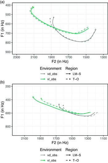
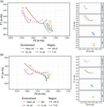


 Open access