


1. Introduction
The study of the wake produced by either a moving body on the surface of water or for flow over a topographic obstacle is a classical problem in fluid dynamics. The observed v-shaped wake pattern is a rare example of a fluid dynamics phenomenon that is well known to everyone. Attempting to minimise or even eliminate the Kelvin wake presents an important problem since in many applications its presence leads to undesirable consequences. For example, it can cause erosion to waterways and river banks (e.g. Bishop Reference Bishop2004), and the wave drag it produces limits the fuel efficiency of boats and ships (Havelock Reference Havelock1908a ).
The mathematical description of the three-dimensional Kelvin wake has been well known for over a century (Kelvin Reference Kelvin1887). Typically, a moving body such as a ship is represented by a pressure disturbance that propagates over the fluid surface. The angle subtended by the characteristic v-shape bounding the linear surface disturbance is usually referred to as the Kelvin wedge angle and is herein denoted by $\theta _{{k}}$
. Another way to measure the wake angle is to measure when the amplitude of the wave peaks reach a certain percentile of the highest wave Darmon, Benzaquen & Raphaël (Reference Darmon, Benzaquen and Raphaël2014), Pethiyagoda et al. (Reference Pethiyagoda, Moroney, Lustri and McCue2021) or by fitting a line to the peaks of the highest downstream waves (Pethiyagoda, McCue & Moroney Reference Pethiyagoda, McCue and Moroney2014; Miao & Liu Reference Miao and Liu2015; Pethiyagoda et al. Reference Pethiyagoda, Moroney, Lustri and McCue2021); both of these methods are used to calculate a so-called ‘apparent’ wake angle, which we emphasise differs from
$\theta _{{k}}$
. Another way to measure the wake angle is to measure when the amplitude of the wave peaks reach a certain percentile of the highest wave Darmon, Benzaquen & Raphaël (Reference Darmon, Benzaquen and Raphaël2014), Pethiyagoda et al. (Reference Pethiyagoda, Moroney, Lustri and McCue2021) or by fitting a line to the peaks of the highest downstream waves (Pethiyagoda, McCue & Moroney Reference Pethiyagoda, McCue and Moroney2014; Miao & Liu Reference Miao and Liu2015; Pethiyagoda et al. Reference Pethiyagoda, Moroney, Lustri and McCue2021); both of these methods are used to calculate a so-called ‘apparent’ wake angle, which we emphasise differs from $\theta _{{k}}$
.
$\theta _{{k}}$
.
In deep water $\theta _{{k}}$
can be found using a linear simplification of the full Euler system on the assumption that the disturbance to the surface is small. Treating the external moving-pressure distribution as a point disturbance leads to Kelvin’s famous result that, in a fluid of infinite depth,
$\theta _{{k}}$
can be found using a linear simplification of the full Euler system on the assumption that the disturbance to the surface is small. Treating the external moving-pressure distribution as a point disturbance leads to Kelvin’s famous result that, in a fluid of infinite depth, $\tan ^2\theta _k = 1/8$
yielding
$\tan ^2\theta _k = 1/8$
yielding $\theta _{{k}}\approx 19.47^\circ$
, which is independent of the speed of the moving-pressure distribution (see, for example, Whitham Reference Whitham1974). Rabaud & Moisy (Reference Rabaud and Moisy2013) worked with a Froude number based on the hull length
$\theta _{{k}}\approx 19.47^\circ$
, which is independent of the speed of the moving-pressure distribution (see, for example, Whitham Reference Whitham1974). Rabaud & Moisy (Reference Rabaud and Moisy2013) worked with a Froude number based on the hull length $L$
, and excluded waves with wavenumbers smaller than a threshold value, reflecting the fact that a ship of length
$L$
, and excluded waves with wavenumbers smaller than a threshold value, reflecting the fact that a ship of length $L$
cannot excite waves of wavelength much larger than
$L$
cannot excite waves of wavelength much larger than $L$
. Later, Noblesse et al. (Reference Noblesse, He, Zhu, Hong, Zhang, Zhu and Yang2014) allowed for interference between the bow and stern of a ship and demonstrated that the apparent wake angle can be smaller than
$L$
. Later, Noblesse et al. (Reference Noblesse, He, Zhu, Hong, Zhang, Zhu and Yang2014) allowed for interference between the bow and stern of a ship and demonstrated that the apparent wake angle can be smaller than $19.47^\circ$
. In shallow water
$19.47^\circ$
. In shallow water $\theta _{{k}}$
also depends on the flow speed and water depth (Havelock Reference Havelock1908b
) and is characterised by a depth-based Froude number,
$\theta _{{k}}$
also depends on the flow speed and water depth (Havelock Reference Havelock1908b
) and is characterised by a depth-based Froude number, $Fr$
, to be defined in (2.4). Herein, unless otherwise explicitly stated, when we refer to the Froude number we mean the depth-based Froude number defined in (2.4).
$Fr$
, to be defined in (2.4). Herein, unless otherwise explicitly stated, when we refer to the Froude number we mean the depth-based Froude number defined in (2.4).
Despite the ubiquity of the Kelvin wake phenomenon and the large number of research articles that have been devoted to it, it remains a topic of considerable scientific interest. Concentrating initially on linear theory, the so-called ‘wave-drag coefficient’ (Havelock Reference Havelock1908a ,Reference Havelock b ; Pedersen Reference Pedersen1988; Li & Ellingsen Reference Li and Ellingsen2016) can be used to quantify the resistance induced by the wake of a moving-pressure distribution in finite depth. In finite depth, the wave pattern induced by mono-hulls and catamarans has been characterised by models using point sources as surface pressure distributions (Zhu et al. Reference Zhu, He, Zhang, Wu, Wan, Zhu and Noblesse2015, Reference Zhu, Ma, Wu, He, Zhang, Li and Noblesse2016) and Hogner ship theory (Zhu et al. Reference Zhu, Wu, He, Zhang, Li and Noblesse2018). There has also been work done to quantify the ‘apparent’ wake angle for an arbitrary pressure distribution in infinite depth (Miao & Liu Reference Miao and Liu2015). In none of these studies did the wave pattern completely disappear for any choice of external forcing.
Theoretical progress has also been made for slow-moving boats in infinite depth assuming the Froude number is small. Somewhat surprisingly, an asymptotic solution of the two-dimensional Euler system, which utilises expansions in powers of the hull-based Froude number, produces no waves at each order of approximation. This apparent paradox can be resolved by resorting to ‘beyond-all-orders’ asymptotics, and in this context, it can be shown that there are waves present downstream that are exponentially small in the Froude number (Trinh, Chapman & Vanden-Broeck Reference Trinh, Chapman and Vanden-Broeck2011; Trinh & Chapman Reference Trinh and Chapman2014). For the two-dimensional problem, Trinh et al. (Reference Trinh, Chapman and Vanden-Broeck2011) showed that downstream waves cannot be eliminated for a single-cornered ship. However, Trinh & Chapman (Reference Trinh and Chapman2014) were not able to make such a conclusive statement for more general piecewise-linear hulls and they did not discount the possibility of wave-free solutions. Lustri & Chapman (Reference Lustri and Chapman2013) and Pethiyagoda et al. (Reference Pethiyagoda, Moroney, Lustri and McCue2021) considered the linear three-dimensional problem for infinite-depth flow over submerged sources and moving-pressure distributions and characterised the ‘apparent’ angle in terms of the system parameters.
In contrast, the fully nonlinear problem has received far less attention in the literature. From a computational perspective, recently, Pethyagoda et al. (Reference Pethiyagoda, McCue and Moroney2014, Reference Pethiyagoda, McCue and Moroney2015) and Buttle et al. (Reference Buttle, Pethiyagoda, Moroney and McCue2018) used a numerical boundary-integral approach coupled with Newton–Krylov and pre-conditioning techniques to solve the fully nonlinear Euler system for inviscid, irrotational flow (hereinafter referred to as the Euler system) in order to capture efficiently the steady wave patterns behind a moving object, and provided important insight into the nonlinear wave drag. Significantly, in infinite depth, Pethiyagoda et al. (Reference Pethiyagoda, McCue and Moroney2014, Reference Pethiyagoda, McCue and Moroney2015) showed that as the flow speed and forcing pressure amplitude are increased, nonlinearity, via the amplitude of the external forcing, alters the ‘apparent’ wake angle and therefore the physical extent of the wavy region. More recently, nonlinear wake patterns have been computed in finite depth by Buttle et al. (Reference Buttle, Pethiyagoda, Moroney and McCue2018), where it was demonstrated that, whilst the linear downstream wave patterns are identical for the moving-pressure problem and the topographic-obstacle problem, the nonlinear wave patterns are different.
The theoretical literature on the fully nonlinear problem is sparse. However, recently, as a first step towards examining the Euler system, Kataoka & Akylas (Reference Kataoka and Akylas2023) showed how an exponential asymptotics approach may be used for smooth boat hulls in the context of a model equation. Examining smooth hulls is important as they can be used to model the bulbous hull shapes that are known to minimise wave drag (see, for example, Grosenbaugh & Yeung Reference Grosenbaugh and Yeung1989). However, modelling smooth bodies moving at arbitrary speeds using the Euler system remains an open challenge.
In this paper, we work towards the goal of eliminating the Kelvin wake behind a moving body in a real flow by studying (i) the simplified model Kadomtsev–Petviashvili equation with a localised forcing term, originally derived by Katsis & Akylas (Reference Katsis and Akylas1987), and it is hereinafter referred to as fKP and (ii) the fully nonlinear Euler system with either a moving-pressure distribution on the surface or a topographic obstacle on the bottom. In the fKP model, we demonstrate that a generic forcing produces a trailing wave pattern similar to that found for the Euler system with a v-shaped wake whose angle we characterise as a function of the Froude number. This includes the critical case $Fr=1$
covered by Katsis & Akylas (Reference Katsis and Akylas1987), which showed that the wake fills the entire region behind the disturbance for this flow speed.
$Fr=1$
covered by Katsis & Akylas (Reference Katsis and Akylas1987), which showed that the wake fills the entire region behind the disturbance for this flow speed.
Furthermore, we use a simple mathematical argument to show that, for the fKP system, it is possible to eliminate the wake. By a judicious choice of forcing function, we construct exact solutions for the fKP model and numerical solutions for the fully nonlinear Euler system for which the disturbance to the water surface is localised around the forcing so that the surface is undisturbed in all directions into the far field. We refer to such solutions as wave-free solutions. Strikingly, we provide evidence that the wave-free solutions are stable, meaning that they are reached in the long-time limit of an initial-value problem (IVP), leading to the possibility of observing them in a physical experiment.
We proceed as follows. In § 2 we describe the problem statement including the fully nonlinear Euler system and the fKP equation and boundary conditions. Then in § 3, we characterise the v-shaped Kelvin wake pattern that emerges for a generic choice of forcing function in the fKP model. In § 4 we discuss how to construct a wave-free steady state for the fKP model and the fully nonlinear Euler system in the presence of a suitably chosen localised forcing. In § 5 we formulate and solve numerically an IVP for the fKP model and fully nonlinear Euler system, to show that the wave-free states are stable. Finally, in § 6 we present our findings and highlight future directions for study.
2. Problem formulation
Before discussing our results we first describe the governing equations; first, the fully nonlinear Euler system and then the fKP model equation. We also illustrate how the dispersion relation for the model fKP agrees with the fully nonlinear Euler system.
2.1. The fully nonlinear Euler system
The fully nonlinear free-surface Euler equations in finite depth are derived from the Navier–Stokes equations under the assumptions of incompressibility, irrotationality and zero viscosity. In figure 1 we show the physical (dimensional) domain and the labelling of the domain and boundaries. To arrive at our non-dimensional system we scale all lengths by the depth of the fluid, $H$
, all velocities by the speed of the incoming uniform flow,
$H$
, all velocities by the speed of the incoming uniform flow, $U$
, and time is scaled by
$U$
, and time is scaled by $H/U$
. If we define
$H/U$
. If we define $\boldsymbol{x}=[x,y]^{\rm T}$
, then the fully nonlinear set of equations for the non-dimensionalised velocity potential
$\boldsymbol{x}=[x,y]^{\rm T}$
, then the fully nonlinear set of equations for the non-dimensionalised velocity potential $\phi (x,y,z)$
and free-surface
$\phi (x,y,z)$
and free-surface $\boldsymbol{r} = [x,y,z_{{f}}(\boldsymbol{x})]^{\rm T}$
are therefore
$\boldsymbol{r} = [x,y,z_{{f}}(\boldsymbol{x})]^{\rm T}$
are therefore
 \begin{align} &\nabla ^2\phi = 0, \quad \boldsymbol{x}\in \mathbb{R}^2,\quad 0\lt z\lt z_{{f}}(\boldsymbol{x}), \end{align}
 \begin{align} &\boldsymbol{r}_t\cdot \boldsymbol{n}_1 = \nabla \phi \cdot \boldsymbol{n}_1,\quad \mbox{on}\quad z = z_{{f}}(\boldsymbol{x}), \end{align}
 \begin{align} &\phi _{t} + \frac {1}{2}|\nabla \phi |^2 + \frac {1}{Fr^2}z_{{f}} + \sigma _{{press}}(\boldsymbol{x})= \frac {1}{2} + \frac {1}{Fr^2},\quad \mbox{on}\quad z = z_{{f}}(\boldsymbol{x}) , \end{align}
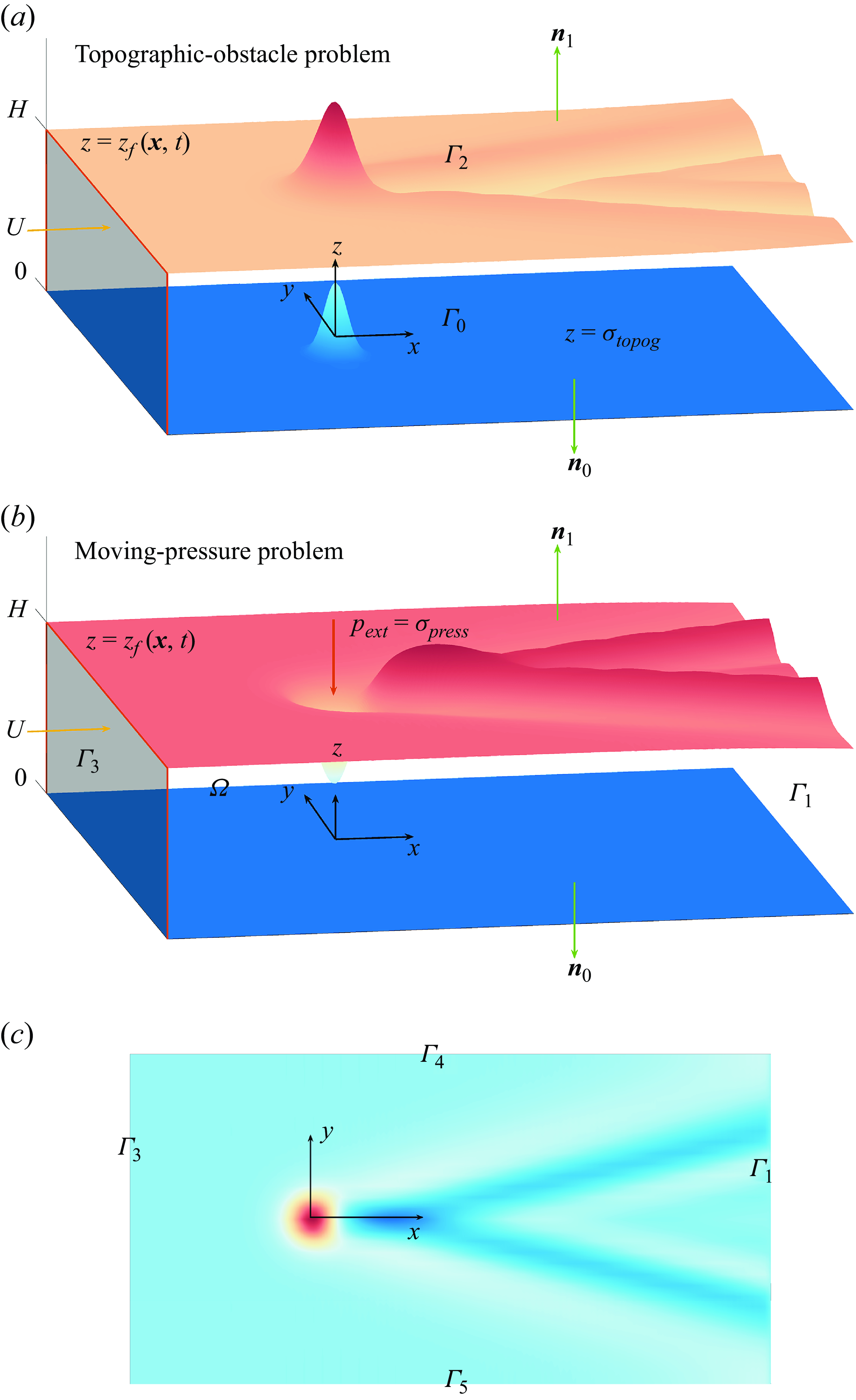
A sketch of the physical (dimensional) domain and labelling of the domain and boundaries. The (a) panel shows the topographic-obstacle problem, the (b) panel shows the moving-pressure problem and the (c) panel shows a plan view of the free surface to demonstrate the boundary labelling. Here, $\Omega$
is the fluid domain,
$\Omega$
is the fluid domain, $\Gamma _0$
is the bottom topography,
$\Gamma _0$
is the bottom topography, $\Gamma _2$
is the free surface,
$\Gamma _2$
is the free surface, $\Gamma _1/\Gamma _3$
are the downstream/upstream faces of the boundary respectively and
$\Gamma _1/\Gamma _3$
are the downstream/upstream faces of the boundary respectively and $\Gamma _4$
and
$\Gamma _4$
and $\Gamma _5$
are the two lateral faces of the boundary.
$\Gamma _5$
are the two lateral faces of the boundary.
where $\sigma _{{press}}(\boldsymbol{x})$
is an imposed pressure distribution on
$\sigma _{{press}}(\boldsymbol{x})$
is an imposed pressure distribution on $z=z_{{f}}(\boldsymbol{x})$
and
$z=z_{{f}}(\boldsymbol{x})$
and $\boldsymbol{n}_1$
is the outwards-pointing unit normal at the free surface and the depth-based Froude number is defined as
$\boldsymbol{n}_1$
is the outwards-pointing unit normal at the free surface and the depth-based Froude number is defined as
 \begin{equation} Fr = \frac {U}{\sqrt {gH}}, \end{equation}
with $U$
and
$U$
and $H$
are the undisturbed physical flow speed and channel height far upstream and
$H$
are the undisturbed physical flow speed and channel height far upstream and $g$
is the gravitational constant (see, for example, Lannes Reference Lannes2013). To close the system we impose
$g$
is the gravitational constant (see, for example, Lannes Reference Lannes2013). To close the system we impose
 \begin{equation} \phi \to x,\quad z_{{f}}\to 1,\quad \mbox{as}\quad x\to -\infty ,\quad \mbox{and}\quad y\to \pm \infty ,\end{equation}
and on the bottom we impose a no-penetration condition
 \begin{equation} \nabla \phi \cdot \boldsymbol{n}_0 = 0,\quad \mbox{on}\quad z = \sigma _{{topog}}(\boldsymbol{x}), \end{equation}
where $\sigma _{{topog}}(\boldsymbol{x})$
is the shape of the topographic distribution and
$\sigma _{{topog}}(\boldsymbol{x})$
is the shape of the topographic distribution and $\boldsymbol{n}_0$
is the outwards-pointing unit normal on the bottom. Furthermore, we define the perturbation to the free surface from its undisturbed upstream height as
$\boldsymbol{n}_0$
is the outwards-pointing unit normal on the bottom. Furthermore, we define the perturbation to the free surface from its undisturbed upstream height as
 \begin{equation} \eta _{{f}}(\boldsymbol{x}) = z_{{f}}(\boldsymbol{x})-1. \end{equation}
The nonlinear system described by (2.1)–(2.6) is what shall be referred to as the fully nonlinear Euler system. In what follows we shall refer to (i) the ‘moving-pressure problem’ which only considers the surface pressure and so $\sigma _{{topog}}=0$
or (ii) the ‘topographic-obstacle problem’ which only considers an obstacle over an underlying uniform stream and so
$\sigma _{{topog}}=0$
or (ii) the ‘topographic-obstacle problem’ which only considers an obstacle over an underlying uniform stream and so $\sigma _{{press}} = 0$
. In both scenarios, we work in a fixed reference frame in which the forcing is stationary and the Bernoulli constant in (2.3) is
$\sigma _{{press}} = 0$
. In both scenarios, we work in a fixed reference frame in which the forcing is stationary and the Bernoulli constant in (2.3) is $1/2 + 1/Fr^2$
.
$1/2 + 1/Fr^2$
.
2.2. The weakly nonlinear model
As derived in the context of water waves the fKP is a partial differential equation (PDE) for the height of the free surface, denoted $\eta (\boldsymbol{x},t)$
, in terms of an external forcing profile,
$\eta (\boldsymbol{x},t)$
, in terms of an external forcing profile, $\sigma (\boldsymbol{x})$
that either represents a surface pressure distribution,
$\sigma (\boldsymbol{x})$
that either represents a surface pressure distribution, $\sigma _{{p}}$
(Katsis & Akylas Reference Katsis and Akylas1987), or the shape of a topographic obstacle,
$\sigma _{{p}}$
(Katsis & Akylas Reference Katsis and Akylas1987), or the shape of a topographic obstacle, $\sigma _{{t}}$
(Keeler Reference Keeler2014). It is derived from (2.1)–(2.6) under the assumptions of (i) shallow water, (ii) small forcing amplitude, (iii) weak
$\sigma _{{t}}$
(Keeler Reference Keeler2014). It is derived from (2.1)–(2.6) under the assumptions of (i) shallow water, (ii) small forcing amplitude, (iii) weak $y$
-dependence and (iv)
$y$
-dependence and (iv) $Fr\approx 1$
(see, for example, Lannes Reference Lannes2013, for mathematically rigorous statements on the validity of this model). Therefore, in contrast to the small-
$Fr\approx 1$
(see, for example, Lannes Reference Lannes2013, for mathematically rigorous statements on the validity of this model). Therefore, in contrast to the small- $Fr$
literature stated in the introduction, our focus is on moderate and fast flow speeds. The equation is
$Fr$
literature stated in the introduction, our focus is on moderate and fast flow speeds. The equation is
 \begin{equation} \left (\eta _t + (Fr - 1)\eta _x - \frac {3}{2}\eta \eta _x - \frac {1}{6}\eta _{xxx} - \frac {1}{2}\sigma _x\right )_x-\frac {1}{2}\eta _{yy} = 0,\quad x,y\in \mathbb{R}, \end{equation}
where the subscripts indicate partial derivatives. Far upstream of the forcing, we impose the boundary conditions
 \begin{align} &\eta ,\eta _x,\eta _{xx},\eta _{xxx}\to 0,\quad \mbox{as} \quad x\to -\infty , \end{align}
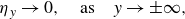 \begin{align} &\eta _y \to 0,\quad \mbox{as}\quad y \to \pm \infty , \end{align}
in accordance with (2.5). We note that (2.8) is valid in the context of no/weak surface tension, and is a modification of the Kadomtsev–Petviashvili II equation (the KPI equation has the opposite sign on the fourth derivative and is for strong surface tension).
It is worth making the link between the fKP model and the fully nonlinear Euler system explicit by examining the linear far-field wave behaviour in the absence of forcing. Substituting $\phi = x + \varepsilon\, \mbox {exp}(\mathrm{i}(\omega t - \boldsymbol{k}\cdot\boldsymbol{x})$
and
$\phi = x + \varepsilon\, \mbox {exp}(\mathrm{i}(\omega t - \boldsymbol{k}\cdot\boldsymbol{x})$
and $z_{{f}} =1 + \varepsilon \, \mbox{exp}(\mathrm{i}(\omega t -\boldsymbol{k}\cdot \boldsymbol{x}))$
, with
$z_{{f}} =1 + \varepsilon \, \mbox{exp}(\mathrm{i}(\omega t -\boldsymbol{k}\cdot \boldsymbol{x}))$
, with $\varepsilon \ll 1$
and
$\varepsilon \ll 1$
and $\boldsymbol{k}=[k_x,k_y]^{\rm T}$
in (2.1)–(2.6) and truncating the system at
$\boldsymbol{k}=[k_x,k_y]^{\rm T}$
in (2.1)–(2.6) and truncating the system at $O(\varepsilon )$
gives the linear dispersion relation of the Euler system in finite depth with an underlying uniform flow. We can also derive a linear dispersion relation for the fKP model (2.8) by assuming
$O(\varepsilon )$
gives the linear dispersion relation of the Euler system in finite depth with an underlying uniform flow. We can also derive a linear dispersion relation for the fKP model (2.8) by assuming $\sigma = 0$
and neglecting nonlinear terms. Written together, these are
$\sigma = 0$
and neglecting nonlinear terms. Written together, these are
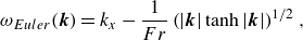 \begin{align} &\omega _{{Euler}}(\boldsymbol{k}) = k_x - \frac {1}{Fr}\left (|\boldsymbol{k}|\tanh |\boldsymbol{k}|\right )^{1/2}, \end{align}
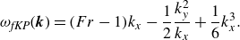 \begin{align} &\omega _{\textit{fKP}}(\boldsymbol{k}) = (Fr-1) k_x - \frac {1}{2}\frac {k_y^2}{k_x} + \frac {1}{6}k_x^3 .\end{align}
By insisting that (i) $Fr$
is close to unity and the waves are (ii) long wavelength, (iii) act on a long time scale and (iv) extend weakly in the transverse direction, it can be deduced that on writing, for constant
$Fr$
is close to unity and the waves are (ii) long wavelength, (iii) act on a long time scale and (iv) extend weakly in the transverse direction, it can be deduced that on writing, for constant $\mu$
,
$\mu$
,
 \begin{equation} k_x\mapsto \mu k_x,\quad k_y\mapsto \mu ^2 k_y,\quad \omega \mapsto \mu ^{3}\omega ,\quad Fr \mapsto 1 + \mu ^2\lambda , \end{equation}
and assuming that $\mu \ll 1$
, then
$\mu \ll 1$
, then $\omega _{{Euler}}$
becomes
$\omega _{{Euler}}$
becomes
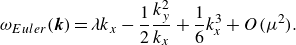 \begin{equation} \omega _{{Euler}}(\boldsymbol{k}) = \lambda k_x - \frac {1}{2}\frac {k_y^2}{k_x} + \frac {1}{6}k_x^3 + O(\mu ^2). \end{equation}
Evidently, at leading order, (2.14) precisely coincides with the dispersion relation of the fKP in (2.12) once the scalings in (2.13) have been reversed.
In the analysis that follows, we will construct a mixture of exact nonlinear steady solutions to (2.8) and numerical steady/unsteady solutions to (2.8) and (2.1)–(2.6). The numerical solutions in both the fKP system and Euler system are found using a finite-element discretisation of the weak form of these systems, as described in Appendix A1). The discretisation of the weak form of the Euler system is discussed in considerable detail in Keeler & Blyth (Reference Keeler and Blyth2024) for the two-dimensional problem; indeed, an attractive feature of this novel numerical framework is that the extension of the problem from two to three spatial dimensions is as trivial as changing a ‘2’ to a ‘3’ in a significant majority of the code.
Finally, it is worth re-emphasising that, in the calculations that follow, we label nonlinear solutions to the fKP equation by $\eta (\boldsymbol{x},t)$
and the perturbed free surface in the fully nonlinear system by
$\eta (\boldsymbol{x},t)$
and the perturbed free surface in the fully nonlinear system by $\eta _{{f}}(\boldsymbol{x},t)$
, see (2.7). We will also use a subscript
$\eta _{{f}}(\boldsymbol{x},t)$
, see (2.7). We will also use a subscript $\ell$
to denote a linear steady solution in either system.
$\ell$
to denote a linear steady solution in either system.
3. Preliminary analysis: weakly nonlinear steady Kelvin wake patterns
Before we demonstrate how we construct wave-free solutions, it is instructive to characterise the v-shaped Kelvin wake pattern using the weakly nonlinear fKP model, and in particular the wedge angle, for a generically chosen external forcing in terms of the flow speed, characterised by the depth-based Froude number, $Fr$
. The procedure we follow is well known for the linearised Euler system (see, for example, Havelock Reference Havelock1908a
,Reference Havelock
b
; Miao & Liu Reference Miao and Liu2015) and has recently been reconstructed for a different model PDE by Kataoka & Akylas (Reference Kataoka and Akylas2023) that models pressure distributions in infinite depth.
$Fr$
. The procedure we follow is well known for the linearised Euler system (see, for example, Havelock Reference Havelock1908a
,Reference Havelock
b
; Miao & Liu Reference Miao and Liu2015) and has recently been reconstructed for a different model PDE by Kataoka & Akylas (Reference Kataoka and Akylas2023) that models pressure distributions in infinite depth.
We emphasise that we were unable to find any explicit analysis for the Kelvin wedge angle in (2.8) in the literature, but note the linear analysis of Katsis & Akylas (Reference Katsis and Akylas1987); restricted to critical flow, $Fr=1$
, and a time-dependent response with no explicit determination of the Kelvin wedge angle as a function of
$Fr=1$
, and a time-dependent response with no explicit determination of the Kelvin wedge angle as a function of $Fr$
. Furthermore, this analysis will reveal simple closed-form expressions for the wedge angle
$Fr$
. Furthermore, this analysis will reveal simple closed-form expressions for the wedge angle $\theta _{{k}}$
as a function of
$\theta _{{k}}$
as a function of $Fr$
and motivate how to eliminate the waves in subsequent sections.
$Fr$
and motivate how to eliminate the waves in subsequent sections.
To determine the Kelvin wedge angle, we examine linear steady solutions to (2.8) by assuming $\eta$
is small
$\eta$
is small
 \begin{equation} \mathcal{L}(\eta _{\ell })= 3\sigma _{\ell ,xx},\quad \mathcal{L} \equiv 6(Fr-1)\partial _{xx} - \partial _{xxxx} - 3\partial _{yy} = 0. \end{equation}
For convenience, in what follows, $\eta _{\ell },\sigma _{\ell }$
correspond to a linear solution and forcing term of (3.1), while
$\eta _{\ell },\sigma _{\ell }$
correspond to a linear solution and forcing term of (3.1), while $\eta ,\sigma$
correspond to a nonlinear solution and forcing term of (2.8). A primary advantage of using the fKP model as opposed to the fully nonlinear Euler system is that, given a linear solution
$\eta ,\sigma$
correspond to a nonlinear solution and forcing term of (2.8). A primary advantage of using the fKP model as opposed to the fully nonlinear Euler system is that, given a linear solution $\eta _{\ell }$
corresponding to a forcing
$\eta _{\ell }$
corresponding to a forcing $\sigma _{\ell }$
, then a nonlinear steady solution can be written down exactly as
$\sigma _{\ell }$
, then a nonlinear steady solution can be written down exactly as
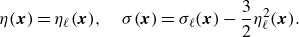 \begin{equation} \eta (\boldsymbol{x}) = \eta _{\ell }(\boldsymbol{x}),\quad \sigma (\boldsymbol{x}) = \sigma _{\ell }(\boldsymbol{x}) - \frac {3}{2}\eta _{{\ell }}^2(\boldsymbol{x}). \end{equation}
We emphasise that, in the fully nonlinear Euler system, we are unable to write down a simple closed-form expression for the nonlinear solution in this fashion.
Returning to the linear problem, we solve (3.1) using the two-dimensional Fourier transform, defined as
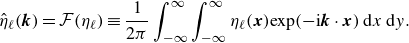 \begin{equation} \hat {\eta }_{\ell }(\boldsymbol{k}) = \mathcal{F}(\eta _{\ell }) \equiv \frac {1}{2\pi }\int _{-\infty }^{\infty }\int _{-\infty }^{\infty }\eta _{\ell }(\boldsymbol{x}) \mbox{exp} (-\mathrm{i}\boldsymbol{k}\cdot \boldsymbol{x})\,\mbox{d}x\,\mbox{d}y. \end{equation}
Introducing a polar coordinate system
 \begin{equation} \boldsymbol{x} = r[\cos \theta ,\sin \theta ]^{\rm T},\quad \boldsymbol{k} = \kappa [\cos \varphi ,\sin \varphi ]^{\rm T} ,\end{equation}
and letting $\hat {\sigma }_{\ell }(\boldsymbol{k}) = \mathcal{F}(\sigma )$
, the steady linear solution to (3.1) can be written in terms of the inverse Fourier transform as
$\hat {\sigma }_{\ell }(\boldsymbol{k}) = \mathcal{F}(\sigma )$
, the steady linear solution to (3.1) can be written in terms of the inverse Fourier transform as
 \begin{equation} \eta _{\ell }(\boldsymbol{x}) = \frac {1}{2\pi } \!\int _{0}^{2\pi } \!\int _{0}^{\infty }\frac {3\hat {\sigma }_{\ell }(\boldsymbol{k})\,\kappa \,\mbox{exp}(\mathrm{i}\kappa r\cos (\varphi -\theta ))}{(\kappa ^2-\kappa _0^2)\cos ^2\varphi }\,\mbox{d}\kappa \,\mbox{d}\varphi ,\,\,\, \kappa _0^2 = \frac {3\tan ^2\varphi - 6(Fr-1)}{\cos ^2\varphi }. \end{equation}
The Kelvin wedge angle can be determined by examining the leading-order asymptotic behaviour of (3.5) far downstream, as $r\to \infty$
,
$r\to \infty$
, $|\theta |\lt \pi /2$
. To proceed, the inner
$|\theta |\lt \pi /2$
. To proceed, the inner $\kappa$
-integration can be achieved by extending the domain of integration into the complex plane, i.e.
$\kappa$
-integration can be achieved by extending the domain of integration into the complex plane, i.e. $\kappa \in \mathbb{C}$
, and then using Cauchy’s residue theorem. For subcritical and critical flow,
$\kappa \in \mathbb{C}$
, and then using Cauchy’s residue theorem. For subcritical and critical flow, $Fr\lt 1$
and
$Fr\lt 1$
and $Fr=1$
, respectively,
$Fr=1$
, respectively, $\kappa _0^2\gt 0$
, and hence there are simple poles at
$\kappa _0^2\gt 0$
, and hence there are simple poles at $\kappa =\pm \kappa _0$
; we only consider the pole at
$\kappa =\pm \kappa _0$
; we only consider the pole at $\kappa =+\kappa _0$
as the integration limit in (3.5) is the positive real line. If
$\kappa =+\kappa _0$
as the integration limit in (3.5) is the positive real line. If $Fr\gt 1$
, it is possible that
$Fr\gt 1$
, it is possible that $\kappa _0^2\lt 0$
and this will be discussed below.
$\kappa _0^2\lt 0$
and this will be discussed below.
Great care has to be taken when choosing the path of integration and choice of contour indentation around the pole $\kappa =+\kappa _0$
which lies directly on the path of integration. Indeed, as remarked in Whitham (Reference Whitham1974) for the fully nonlinear Euler system, there is an ambiguity that stems from the fact that the radiation condition states there cannot be waves upstream. A similar problem arises in (3.5), so to remedy this, we follow Whitham (Reference Whitham1974) and allow
$\kappa =+\kappa _0$
which lies directly on the path of integration. Indeed, as remarked in Whitham (Reference Whitham1974) for the fully nonlinear Euler system, there is an ambiguity that stems from the fact that the radiation condition states there cannot be waves upstream. A similar problem arises in (3.5), so to remedy this, we follow Whitham (Reference Whitham1974) and allow $\eta _{\ell }$
and
$\eta _{\ell }$
and $\sigma _{\ell }$
to be weakly time dependent by mapping
$\sigma _{\ell }$
to be weakly time dependent by mapping
 \begin{equation} \eta _{\ell }(\boldsymbol{x},t) \mapsto \eta _{\ell }(\boldsymbol{x})\mbox{exp}(\delta t),\quad \sigma _{\ell }(\boldsymbol{x},t) \mapsto \sigma _{\ell }(\boldsymbol{x})\mbox{exp}(\delta t), \end{equation}
with $\delta \gt 0$
in (2.8), ignoring the nonlinear term. This mimics the forcing being effectively zero as
$\delta \gt 0$
in (2.8), ignoring the nonlinear term. This mimics the forcing being effectively zero as $t\to -\infty$
, and has the effect of altering
$t\to -\infty$
, and has the effect of altering $\mathcal{L}(\eta _{\ell })$
in (3.1) to
$\mathcal{L}(\eta _{\ell })$
in (3.1) to
 \begin{equation} \mathcal{L}(\eta _{\ell })\mapsto \mathcal{L}(\eta _{\ell }) + 6\delta \eta _{\ell ,x}, \end{equation}
and it can be shown that, now, the pole gets translated into the upper complex plane to
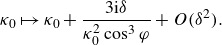 \begin{equation} \kappa _0 \mapsto \kappa _0 + \frac {3\mathrm{i}\delta }{\kappa _0^2\cos ^3\varphi } + O(\delta ^2). \end{equation}
The ambiguity in choosing the orientation of the indentation over the pole is now redundant. Finally, by taking the limit $\delta \to 0^+$
, we recover the steady solution to (3.1).
$\delta \to 0^+$
, we recover the steady solution to (3.1).
Due to this construction, for $\cos (\varphi -\theta )\gt 0$
, we close our path of integration in the upper half complex
$\cos (\varphi -\theta )\gt 0$
, we close our path of integration in the upper half complex $\kappa $
-plane by adding a quarter-circle arc from the positive real
$\kappa $
-plane by adding a quarter-circle arc from the positive real $\kappa$
axis to the positive imaginary
$\kappa$
axis to the positive imaginary $\kappa$
axis and then returning to the origin and the pole will contribute as
$\kappa$
axis and then returning to the origin and the pole will contribute as $r\to \infty$
(we note that the contribution of the integrand on the imaginary axis is exponentially small in
$r\to \infty$
(we note that the contribution of the integrand on the imaginary axis is exponentially small in $r$
). For
$r$
). For $\cos (\varphi -\theta )\lt 0$
the contour gets deformed onto the negative imaginary axis and the pole does not contribute.
$\cos (\varphi -\theta )\lt 0$
the contour gets deformed onto the negative imaginary axis and the pole does not contribute.
Taking the limit $\delta \to 0^+$
, the leading-order asymptotic behaviour of the inner integral, when
$\delta \to 0^+$
, the leading-order asymptotic behaviour of the inner integral, when $\cos (\varphi -\theta ) \gt 0$
in (3.5), is simply the residue of the integrand at
$\cos (\varphi -\theta ) \gt 0$
in (3.5), is simply the residue of the integrand at $\kappa _0$
and therefore
$\kappa _0$
and therefore
 \begin{equation} \eta _{\ell }(\boldsymbol{x}) \sim \frac {3}{2}\mathrm{i}\int _{-\pi /2+\theta }^{\pi /2}\frac {\hat {\sigma }_{{\ell }}(\boldsymbol{k}_0)}{\cos ^2\varphi }\mbox{exp}(\mathrm{i}|\kappa _0| r\cos (\varphi -\theta ))\,\mbox{d}\varphi ,\quad \mbox{as}\quad r\to \infty , \end{equation}
where $\boldsymbol{k}_0 = |\kappa _0|[\cos \varphi ,\sin \varphi ]^{\rm T}$
is dependent on
$\boldsymbol{k}_0 = |\kappa _0|[\cos \varphi ,\sin \varphi ]^{\rm T}$
is dependent on $\varphi$
only. The limits of integration on the outer-
$\varphi$
only. The limits of integration on the outer- $\varphi$
integral have changed from (3.5) as the solution is symmetric about
$\varphi$
integral have changed from (3.5) as the solution is symmetric about $\theta =0$
so we only need to consider
$\theta =0$
so we only need to consider $0\lt \theta \lt \pi$
, which means that, as
$0\lt \theta \lt \pi$
, which means that, as $\cos (\varphi -\theta )\gt 0$
,
$\cos (\varphi -\theta )\gt 0$
, $-\pi /2+\theta \lt \varphi \lt \pi /2$
. The dominant behaviour of the integral as
$-\pi /2+\theta \lt \varphi \lt \pi /2$
. The dominant behaviour of the integral as $r\to \infty$
occurs when the exponent in (3.9) is stationary, i.e.
$r\to \infty$
occurs when the exponent in (3.9) is stationary, i.e.
 \begin{equation} \frac {\partial g}{\partial \varphi } = 0, \: \mbox{where} \: g(\varphi ,\theta ) = \kappa _0\cos (\varphi -\theta )\equiv \frac {\sqrt {3}(\tan ^2\varphi - 2(Fr-1))^{1/2}\cos (\varphi -\theta )}{\cos \varphi }. \end{equation}
The leading-order asymptotic behaviour of (3.9) as $r\to \infty$
is readily obtained using the stationary-phase formula
$r\to \infty$
is readily obtained using the stationary-phase formula
 \begin{equation} \eta _{\ell }(\boldsymbol{x})\sim \frac {3\sqrt {\pi }(\mathrm{i}-\lambda )}{4}\sum _{n}r^{-1/2}\,\frac {\hat {\sigma }_{{\ell }}(\kappa _0,\varphi _n)}{|g''(\varphi _n)|^{1/2}\cos ^2\varphi _n}\mbox{exp}\left [\mathrm{i}|\kappa _0| r\cos (\varphi _n-\theta ) \right ]+ {c.c.}, \end{equation}
where the sum is over the $n$
permissible solutions,
$n$
permissible solutions, $\varphi =\varphi _n$
, of (3.10),
$\varphi =\varphi _n$
, of (3.10), $\lambda = \mbox{sgn}(g''(\varphi _n))$
is the signum function,
$\lambda = \mbox{sgn}(g''(\varphi _n))$
is the signum function, $g''(\varphi _n)$
is the second derivative of
$g''(\varphi _n)$
is the second derivative of $g(\varphi )$
with respect to
$g(\varphi )$
with respect to $\varphi$
,
$\varphi$
, $\hat {\sigma }_{\ell }(\kappa _0,\varphi _n) = \hat {\sigma }_{\ell }(\boldsymbol{k}_0)|_{\varphi = \varphi _n}$
and c.c. stands for complex conjugate. Physically, as can be seen from (3.11),
$\hat {\sigma }_{\ell }(\kappa _0,\varphi _n) = \hat {\sigma }_{\ell }(\boldsymbol{k}_0)|_{\varphi = \varphi _n}$
and c.c. stands for complex conjugate. Physically, as can be seen from (3.11), $\kappa _0$
characterises the wavenumber of the oscillations.
$\kappa _0$
characterises the wavenumber of the oscillations.
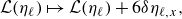
The left, middle and right columns show results for $Fr=0.5,1.0$
and
$Fr=0.5,1.0$
and $2.0$
, respectively. (a)–(c) Nonlinear steady solutions of (2.8) for
$2.0$
, respectively. (a)–(c) Nonlinear steady solutions of (2.8) for $\sigma (\boldsymbol{x}) = a\,\mbox{exp}(-\boldsymbol{x}\cdot \boldsymbol{x})$
with
$\sigma (\boldsymbol{x}) = a\,\mbox{exp}(-\boldsymbol{x}\cdot \boldsymbol{x})$
with $a=0.1$
. The linear Kelvin wedge angle,
$a=0.1$
. The linear Kelvin wedge angle, $\theta _{{k}}$
is indicated as dotted lines. (d)–(f) The roots of (3.10) in the range
$\theta _{{k}}$
is indicated as dotted lines. (d)–(f) The roots of (3.10) in the range $-\pi /2 + \theta \lt \varphi \lt \pi /2$
as a function of
$-\pi /2 + \theta \lt \varphi \lt \pi /2$
as a function of $\theta$
for a general forcing function
$\theta$
for a general forcing function $\sigma _{\ell }$
. (g)–(i) The pole on the real axis,
$\sigma _{\ell }$
. (g)–(i) The pole on the real axis, $\kappa _0$
, evaluated at
$\kappa _0$
, evaluated at $\varphi _{1,2}$
.
$\varphi _{1,2}$
.
When $Fr\neq 1$
the solutions satisfy the quadratic equation for
$Fr\neq 1$
the solutions satisfy the quadratic equation for $\tan \varphi$
,
$\tan \varphi$
,
 \begin{equation} 2\sin \theta \tan ^2\varphi + \cos \theta \tan \varphi - 2(Fr-1) \sin \theta = 0. \end{equation}
Hence, when $Fr\lt 1$
, there are two real solutions for
$Fr\lt 1$
, there are two real solutions for $\varphi$
provided that
$\varphi$
provided that
 \begin{equation} 0\lt |\theta |\lt \theta _{{k}}(Fr),\quad \mbox{where}\quad 16(1 - Fr)\tan ^2\theta _{{k}} = 1. \end{equation}
The value of $\theta _{{k}}(Fr)$
is interpreted as the Kelvin wedge angle. It is indicated by the dashed vertical line in figure 2(d) for the case
$\theta _{{k}}(Fr)$
is interpreted as the Kelvin wedge angle. It is indicated by the dashed vertical line in figure 2(d) for the case $Fr=0.5$
. Comparing the value of
$Fr=0.5$
. Comparing the value of $\kappa _0$
at each root, see figure 2(g), we see that one of the solutions,
$\kappa _0$
at each root, see figure 2(g), we see that one of the solutions, $\varphi _1$
, is short wavelength and corresponds to a so-called divergent wave (that shall be discussed below) whilst the other solution,
$\varphi _1$
, is short wavelength and corresponds to a so-called divergent wave (that shall be discussed below) whilst the other solution, $\varphi _2$
, is long wavelength and corresponds to a so-called transverse wave that oscillates on the line
$\varphi _2$
, is long wavelength and corresponds to a so-called transverse wave that oscillates on the line $\theta =0$
, as can be seen in (3.11). For historical context, the divergent/transverse terminology was first coined in Havelock (Reference Havelock1908b
). We note the special case of
$\theta =0$
, as can be seen in (3.11). For historical context, the divergent/transverse terminology was first coined in Havelock (Reference Havelock1908b
). We note the special case of $Fr=1/2$
, as shown in figure 2(d),(g), which results in
$Fr=1/2$
, as shown in figure 2(d),(g), which results in $\theta _{{k}} = \mathrm{arctan}(1/2\sqrt {2})\approx 19.47^{\circ }$
, the classical Kelvin wedge angle for the linearised Euler system.
$\theta _{{k}} = \mathrm{arctan}(1/2\sqrt {2})\approx 19.47^{\circ }$
, the classical Kelvin wedge angle for the linearised Euler system.


When $Fr\gt 1$
equation (3.12) has two solutions for any
$Fr\gt 1$
equation (3.12) has two solutions for any $0\lt |\theta | \lt \pi /2$
. However, for one of these solutions,
$0\lt |\theta | \lt \pi /2$
. However, for one of these solutions, $\varphi _2$
, we find that
$\varphi _2$
, we find that $\kappa _0^2\lt 0$
for all
$\kappa _0^2\lt 0$
for all $0\lt |\theta | \lt \pi /2$
and so the pole in (3.5) is not on the real axis (as
$0\lt |\theta | \lt \pi /2$
and so the pole in (3.5) is not on the real axis (as $\delta \to 0$
) and does not contribute to the far-field wave pattern. For the other (divergent) solution,
$\delta \to 0$
) and does not contribute to the far-field wave pattern. For the other (divergent) solution, $\varphi _1$
, the transition from
$\varphi _1$
, the transition from $\kappa _0^2\gt 0$
(pole tending to the real axis) to
$\kappa _0^2\gt 0$
(pole tending to the real axis) to $\kappa _0^2\lt 0$
(pole tending to the imaginary axis) occurs when
$\kappa _0^2\lt 0$
(pole tending to the imaginary axis) occurs when $\tan ^2\varphi =2(Fr-1)$
. Inserting the latter into (3.12) we find that the permissible
$\tan ^2\varphi =2(Fr-1)$
. Inserting the latter into (3.12) we find that the permissible $\theta$
are bounded by the Kelvin wedge angle,
$\theta$
are bounded by the Kelvin wedge angle, $\theta _{{k}}$
and satisfy
$\theta _{{k}}$
and satisfy
 \begin{equation} 0\lt |\theta |\lt \theta _{{k}}(Fr),\quad \mbox{where}\quad 2(Fr-1)\tan ^2\theta _{{k}} = 1. \end{equation}
Focusing on $Fr\gt 1$
, a key feature of the divergent wave solution is the presence of a ‘shadow region’ downstream of the forcing where there is minimal surface disturbance, see figure 2(c), and no surface disturbance at
$Fr\gt 1$
, a key feature of the divergent wave solution is the presence of a ‘shadow region’ downstream of the forcing where there is minimal surface disturbance, see figure 2(c), and no surface disturbance at $\theta =0$
. To see this,
$\theta =0$
. To see this, $\varphi _1\to -\pi /2$
and
$\varphi _1\to -\pi /2$
and $\kappa _0\to \infty$
as
$\kappa _0\to \infty$
as $\theta \to 0$
, see figure 2(f,i). Therefore, examining (3.11), for a fixed value of
$\theta \to 0$
, see figure 2(f,i). Therefore, examining (3.11), for a fixed value of $r$
;
$r$
; $\eta _{\ell }$
decays to zero as
$\eta _{\ell }$
decays to zero as $\theta \to 0$
, provided
$\theta \to 0$
, provided $\hat {\sigma }_{\ell }(\kappa _0,\varphi _1)$
decays sufficiently quickly as
$\hat {\sigma }_{\ell }(\kappa _0,\varphi _1)$
decays sufficiently quickly as $\kappa _0\to \infty$
. The Gaussian forcing we choose in the calculations in figure 2(a–c), and discussed below, fulfils this criterion.
$\kappa _0\to \infty$
. The Gaussian forcing we choose in the calculations in figure 2(a–c), and discussed below, fulfils this criterion.
Finally, when $Fr=1$
(3.10) has a unique solution,
$Fr=1$
(3.10) has a unique solution, $\varphi _1$
, corresponding to a divergent wave, for any
$\varphi _1$
, corresponding to a divergent wave, for any $0\lt |\theta |\leqslant \pi /2$
which satisfies
$0\lt |\theta |\leqslant \pi /2$
which satisfies
 \begin{equation} \tan \varphi = -\tfrac {1}{2}\cot \theta . \end{equation}
Hence, the Kelvin wedge angle is $\theta _{{k}} = \pi /2$
, as was first noted in Katsis & Akylas (Reference Katsis and Akylas1987).
$\theta _{{k}} = \pi /2$
, as was first noted in Katsis & Akylas (Reference Katsis and Akylas1987).
In summary, we have determined the far-field Kelvin wedge angle as a function of $Fr$
for subcritical and supercritical flows, as stated in (3.13) and (3.14), respectively. The wedge angle is plotted against
$Fr$
for subcritical and supercritical flows, as stated in (3.13) and (3.14), respectively. The wedge angle is plotted against $Fr$
in figure 3. We note that
$Fr$
in figure 3. We note that $\theta _{{k}}\to \pi /2$
as
$\theta _{{k}}\to \pi /2$
as $Fr\to 1^{\pm }$
and that for large
$Fr\to 1^{\pm }$
and that for large $Fr$
we have the asymptotic behaviour
$Fr$
we have the asymptotic behaviour
 \begin{equation} \theta _{{k}}\sim \, (\sqrt {2}/2)\,Fr^{-1/2}\quad \mbox{as}\quad Fr\to \infty . \end{equation}
This asymptotic behaviour differs from the linearised Euler system where the dependence of the $\theta _{{k}}$
on the flow speed is well known, most notably reported by Havelock (1908b), where it was found that the leading-order asymptotic behaviour for
$\theta _{{k}}$
on the flow speed is well known, most notably reported by Havelock (1908b), where it was found that the leading-order asymptotic behaviour for $Fr\gg 1$
is
$Fr\gg 1$
is $\theta _{{k}}=\mathrm{asin}(Fr^{-1})\sim \,Fr^{-1}$
(more recently noted by Pethiyagoda et al. (Reference Pethiyagoda, Moroney, Macfarlane, Binns and McCue2018)). This discrepancy can be explained by the fact that the fKP is only valid around
$\theta _{{k}}=\mathrm{asin}(Fr^{-1})\sim \,Fr^{-1}$
(more recently noted by Pethiyagoda et al. (Reference Pethiyagoda, Moroney, Macfarlane, Binns and McCue2018)). This discrepancy can be explained by the fact that the fKP is only valid around $Fr\approx 1$
.
$Fr\approx 1$
.
We can compare the values for $\theta _{{k}}$
, obtained from the solution to (3.13) and (3.14), with the numerically computed nonlinear steady wave patterns, found by solving the steady form of the fKP (2.8), as shown in figure 2(a–c) for
$\theta _{{k}}$
, obtained from the solution to (3.13) and (3.14), with the numerically computed nonlinear steady wave patterns, found by solving the steady form of the fKP (2.8), as shown in figure 2(a–c) for $Fr=0.5,1.0,2.0$
, respectively. For concreteness, we choose a Gaussian forcing
$Fr=0.5,1.0,2.0$
, respectively. For concreteness, we choose a Gaussian forcing $\sigma (\boldsymbol{x}) = a\,\mbox{exp}(-\boldsymbol{x}\cdot \boldsymbol{x})$
and
$\sigma (\boldsymbol{x}) = a\,\mbox{exp}(-\boldsymbol{x}\cdot \boldsymbol{x})$
and $a=0.1$
. The dashed lines in each panel indicate the Kelvin wedge angle,
$a=0.1$
. The dashed lines in each panel indicate the Kelvin wedge angle, $\theta _{{k}}$
. This theoretically derived angle shows excellent agreement with the numerically produced nonlinear wave patterns, giving us confidence in our numerical scheme (see Appendix A1). Furthermore, the wave patterns are qualitatively the same as the fully nonlinear solutions reported in Buttle et al. (Reference Buttle, Pethiyagoda, Moroney and McCue2018), where transverse waves are present for
$\theta _{{k}}$
. This theoretically derived angle shows excellent agreement with the numerically produced nonlinear wave patterns, giving us confidence in our numerical scheme (see Appendix A1). Furthermore, the wave patterns are qualitatively the same as the fully nonlinear solutions reported in Buttle et al. (Reference Buttle, Pethiyagoda, Moroney and McCue2018), where transverse waves are present for $Fr\lt 1$
but absent when
$Fr\lt 1$
but absent when $Fr\geqslant 1$
, where instead a ‘shadow region’ appears.
$Fr\geqslant 1$
, where instead a ‘shadow region’ appears.
Although the linear theory for the fully nonlinear Euler system is well established (see, for example, Havelock Reference Havelock1908b
), to our knowledge this is the first time the Kelvin wedge angle and wave pattern have been calculated explicitly for a range of $Fr$
, in the context of the fKP equation and is the first main result of this paper. Due to the simplicity of (3.1), and the fact that we have obtained simple closed-form exact equations for
$Fr$
, in the context of the fKP equation and is the first main result of this paper. Due to the simplicity of (3.1), and the fact that we have obtained simple closed-form exact equations for $\theta _{{k}}$
as a function of
$\theta _{{k}}$
as a function of $Fr$
for subcritical flow, this demonstrates the promising potential of the fKP equation as a ‘sand-pit’ model to understand nonlinear Kelvin wave patterns.
$Fr$
for subcritical flow, this demonstrates the promising potential of the fKP equation as a ‘sand-pit’ model to understand nonlinear Kelvin wave patterns.
Comparison between nonlinear steady surface wave patterns of the fully nonlinear Euler system, $\eta _{{f}}(\boldsymbol{x})$
for a moving-pressure problem, (labelled MP in the top row of each box), topographic-obstacle problem (labelled TO in the middle row of each box) and the fKP model,
$\eta _{{f}}(\boldsymbol{x})$
for a moving-pressure problem, (labelled MP in the top row of each box), topographic-obstacle problem (labelled TO in the middle row of each box) and the fKP model, $\eta (\boldsymbol{x})$
(bottom row in each box) for a range of
$\eta (\boldsymbol{x})$
(bottom row in each box) for a range of $Fr$
and
$Fr$
and $\sigma = a\,\mbox{exp}(-\boldsymbol{x}\cdot \boldsymbol{x})$
. Note that the colour map is different for each panel but the reference values
$\sigma = a\,\mbox{exp}(-\boldsymbol{x}\cdot \boldsymbol{x})$
. Note that the colour map is different for each panel but the reference values $\mbox{min}(\eta ),0$
and
$\mbox{min}(\eta ),0$
and $\mbox{max}(\eta )$
(where applicable) have been labelled on the colour bar for ease of reference. The top box is for
$\mbox{max}(\eta )$
(where applicable) have been labelled on the colour bar for ease of reference. The top box is for $a=0.001$
and the bottom box is for
$a=0.001$
and the bottom box is for $a=0.1$
. All figures are plotted in the range
$a=0.1$
. All figures are plotted in the range $x\in [-20,20],y\in [-20,20]$
.
$x\in [-20,20],y\in [-20,20]$
.
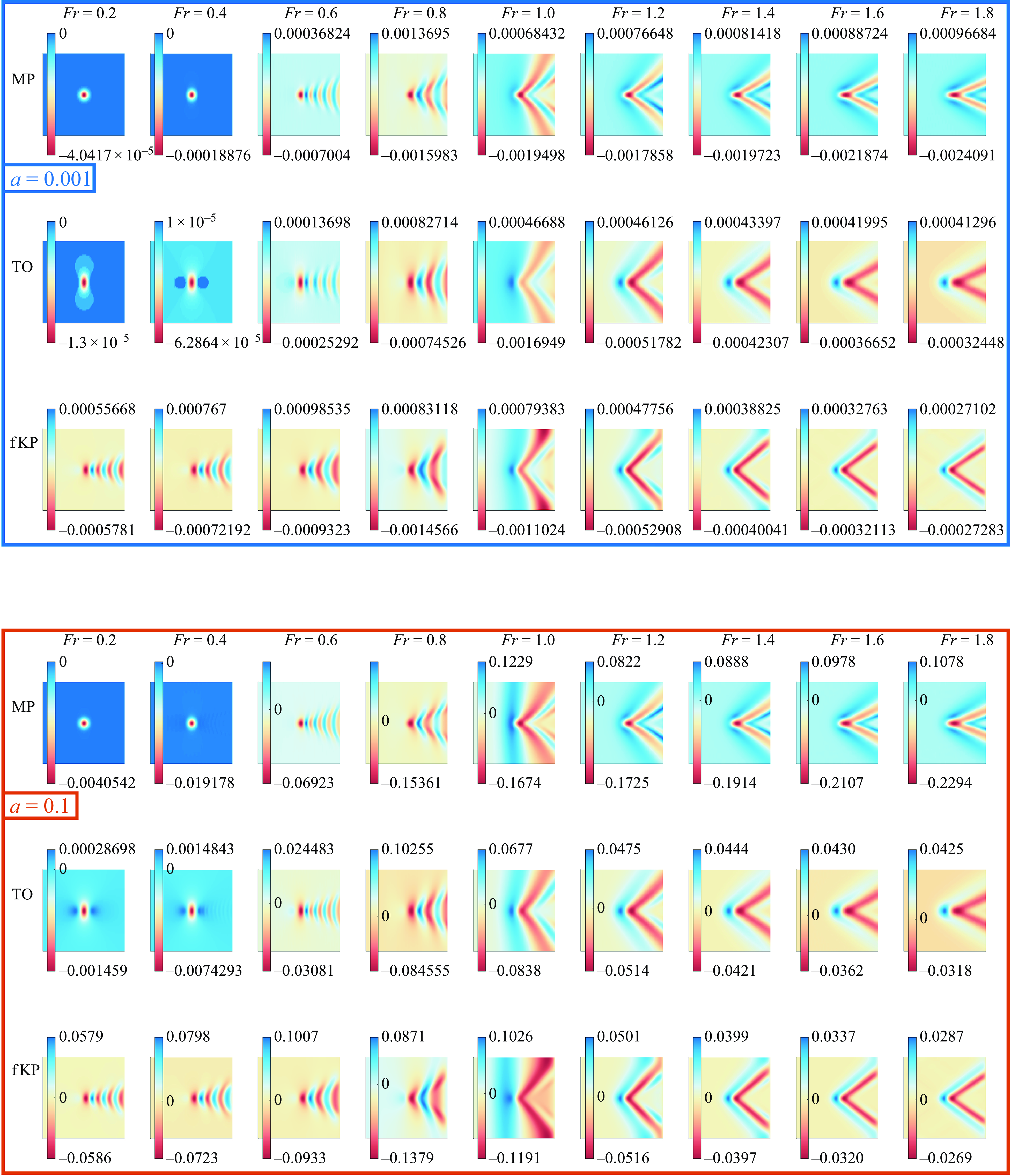
In figure 4 we show a comparison between the fKP model and the fully nonlinear Euler system when $\sigma (\boldsymbol{x}) = a\,\mbox{exp}(-\boldsymbol{x}\cdot \boldsymbol{x})$
for small amplitude forcings (
$\sigma (\boldsymbol{x}) = a\,\mbox{exp}(-\boldsymbol{x}\cdot \boldsymbol{x})$
for small amplitude forcings ( $a=0.001$
, top box) and large amplitude forcings (
$a=0.001$
, top box) and large amplitude forcings ( $a=0.1$
, bottom box). The steady wave patterns,
$a=0.1$
, bottom box). The steady wave patterns, $\eta _{{f}}(\boldsymbol{x})$
, for the fully nonlinear Euler system (top row in each box for the moving-pressure problem, middle row in each box for the topographic-obstacle problem) show good agreement with the fKP steady wave patterns,
$\eta _{{f}}(\boldsymbol{x})$
, for the fully nonlinear Euler system (top row in each box for the moving-pressure problem, middle row in each box for the topographic-obstacle problem) show good agreement with the fKP steady wave patterns, $\eta (\boldsymbol{x})$
, around
$\eta (\boldsymbol{x})$
, around $Fr=1$
. For smaller values of
$Fr=1$
. For smaller values of $Fr$
, the fully nonlinear Euler system appears to exhibit no waves in both the moving-pressure and topographic-obstacle problems but we would expect these waves to be exponentially small in
$Fr$
, the fully nonlinear Euler system appears to exhibit no waves in both the moving-pressure and topographic-obstacle problems but we would expect these waves to be exponentially small in $Fr$
and so hard to detect numerically (Pethiyagoda et al. Reference Pethiyagoda, Moroney, Lustri and McCue2021). We remark that the agreement between the different systems is also good for large amplitude forcings, at least around
$Fr$
and so hard to detect numerically (Pethiyagoda et al. Reference Pethiyagoda, Moroney, Lustri and McCue2021). We remark that the agreement between the different systems is also good for large amplitude forcings, at least around $Fr=1$
.
$Fr=1$
.
An important part of the analysis that we emphasise is the importance of the pole, $\kappa _0$
, in producing waves downstream; if we can eliminate this pole, then there is a possibility that a wave-free steady state could exist. Since
$\kappa _0$
, in producing waves downstream; if we can eliminate this pole, then there is a possibility that a wave-free steady state could exist. Since $\kappa _0$
does not depend on the explicit form of the forcing term,
$\kappa _0$
does not depend on the explicit form of the forcing term, $\sigma (\boldsymbol{x})$
, then the forcing does not play a leading role in determining the wave pattern far downstream. It is often convenient to model
$\sigma (\boldsymbol{x})$
, then the forcing does not play a leading role in determining the wave pattern far downstream. It is often convenient to model $\sigma (\boldsymbol{x})$
, taking the role as a ‘boat’, as a Dirac-delta function or Gaussian for a one-point wavemaker (see, for example, Whitham Reference Whitham1974; Katsis & Akylas Reference Katsis and Akylas1987) or as a dipole modelling a two-point wavemaker (Noblesse et al. Reference Noblesse, He, Zhu, Hong, Zhang, Zhu and Yang2014; Miao & Liu Reference Miao and Liu2015). We will now show that, through a judicious choice of
$\sigma (\boldsymbol{x})$
, taking the role as a ‘boat’, as a Dirac-delta function or Gaussian for a one-point wavemaker (see, for example, Whitham Reference Whitham1974; Katsis & Akylas Reference Katsis and Akylas1987) or as a dipole modelling a two-point wavemaker (Noblesse et al. Reference Noblesse, He, Zhu, Hong, Zhang, Zhu and Yang2014; Miao & Liu Reference Miao and Liu2015). We will now show that, through a judicious choice of ${\sigma }(\boldsymbol{x})$
, corresponding to a localised forcing term, a nonlinear steady wave-free
${\sigma }(\boldsymbol{x})$
, corresponding to a localised forcing term, a nonlinear steady wave-free $\eta (\boldsymbol{x})$
exists.
$\eta (\boldsymbol{x})$
exists.
4. Wave-free steady solutions
4.1. Weakly nonlinear model
Initially, we concentrate on the linear solution (3.5) to the weakly nonlinear fKP model, which in Cartesian coordinates ( $\boldsymbol{k} = [k_x,k_y]^{\rm T}$
) can be written as
$\boldsymbol{k} = [k_x,k_y]^{\rm T}$
) can be written as
 \begin{equation} \eta _{\ell }(\boldsymbol{x}) =\frac {1}{2\pi } \int _{-\infty }^{\infty }\int _{-\infty }^{\infty }\frac {3k_x^2\,\hat {\sigma }_{\ell }(\boldsymbol{k})}{6(Fr-1)k_x^2 + k_x^4 - 3k_y^2}\,\mbox{exp}(\mathrm{i}\boldsymbol{k}\cdot \boldsymbol{x})\,\mbox{d}k_x\,\mbox{d}k_y. \end{equation}
As previously stated, the pole in the integrand is responsible for the far-field wave pattern as $x\to \infty$
. Therefore, an obvious choice for
$x\to \infty$
. Therefore, an obvious choice for $\hat {\sigma }_{\ell }(\boldsymbol{k})$
that eliminates this pole is
$\hat {\sigma }_{\ell }(\boldsymbol{k})$
that eliminates this pole is
 \begin{equation} \hat {\sigma }_{\ell }(\boldsymbol{k}) = \frac {1}{3} \left[6(Fr-1)k_x^2 + k_x^4 - 3k_y^2 \right]\,\hat {f}(\boldsymbol{k}), \end{equation}
where $\hat {f}$
is the Fourier transform of an arbitrary function,
$\hat {f}$
is the Fourier transform of an arbitrary function, $f(\boldsymbol{x})$
, that is localised in physical space. In physical space, the linear solution is
$f(\boldsymbol{x})$
, that is localised in physical space. In physical space, the linear solution is
 \begin{equation} \eta _{\ell }(\boldsymbol{x}) = \frac {1}{2\pi }\int _{-\infty }^{\infty }\int _{-\infty }^{\infty } k_x^2 \hat {f}(\boldsymbol{k})\,\mbox{exp}(\mathrm{i}\boldsymbol{k}\cdot \boldsymbol{x})\,\mbox{d}k_x\,\mbox{d}k_y = -(f(\boldsymbol{x}))_{xx}. \end{equation}
A simple illustrative example is the choice $\hat {f}(\boldsymbol{k}) =-a\,\pi \,\mbox{exp} (-(1/4)\boldsymbol{k}\cdot \boldsymbol{k} ),\, a\in \mathbb{R}.$
In this case, it is straightforward to see from (4.3) that
$\hat {f}(\boldsymbol{k}) =-a\,\pi \,\mbox{exp} (-(1/4)\boldsymbol{k}\cdot \boldsymbol{k} ),\, a\in \mathbb{R}.$
In this case, it is straightforward to see from (4.3) that
 \begin{equation} \eta _{\ell }(\boldsymbol{x}) = a\left (\mbox{exp}(-\boldsymbol{x}\cdot \boldsymbol{x})\right )_{xx}, \end{equation}
which is, crucially, wave free in the far field; thus achieving our goal. Recall that $\eta _{\ell }$
and
$\eta _{\ell }$
and $\sigma _{\ell }$
satisfy (3.1) so, in order to satisfy the nonlinear problem (2.8), we simply insert (4.4) into the relation in (3.2).
$\sigma _{\ell }$
satisfy (3.1) so, in order to satisfy the nonlinear problem (2.8), we simply insert (4.4) into the relation in (3.2).
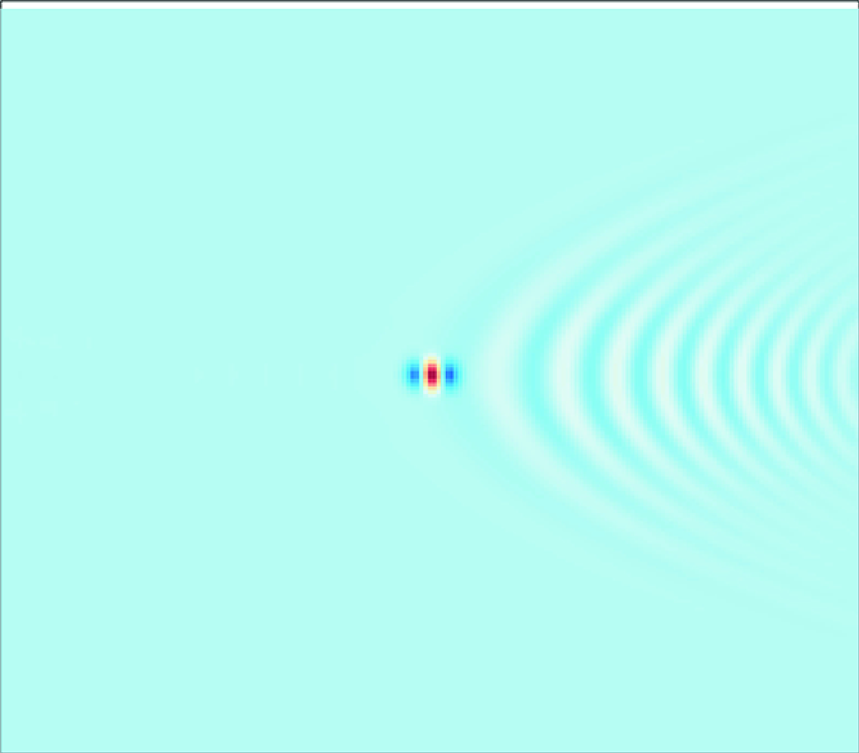
Steady weakly nonlinear wave-free solutions defined in (3.2). Panels (a–b) the nonlinear free surface, $\eta (\boldsymbol{x})$
for
$\eta (\boldsymbol{x})$
for $a=0.1,Fr=1.0$
. Panels (c–d) the forcing,
$a=0.1,Fr=1.0$
. Panels (c–d) the forcing, $\sigma (\boldsymbol{x})$
.
$\sigma (\boldsymbol{x})$
.
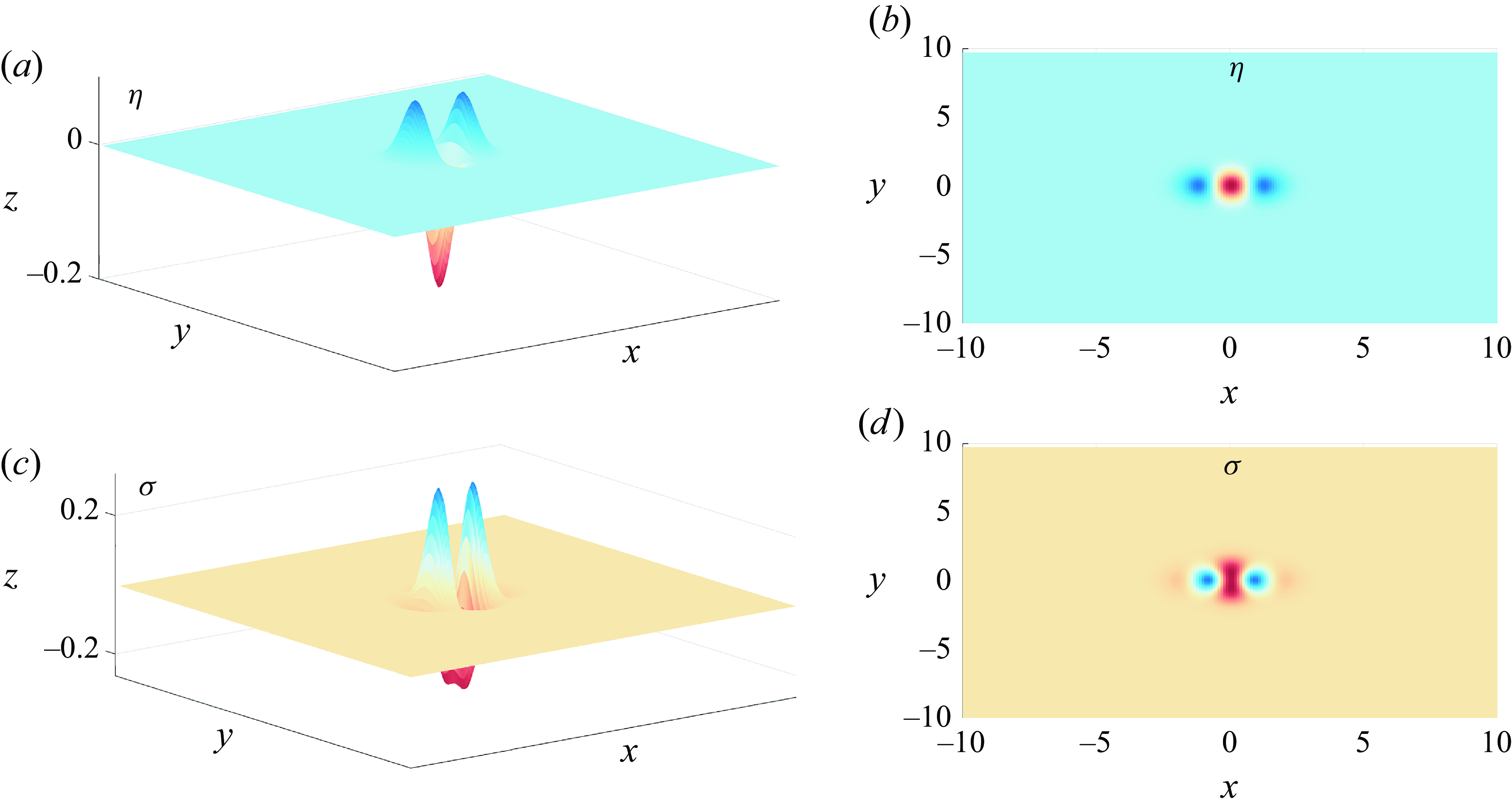
As an example, when $a=0.1,Fr=1.0$
, the nonlinear solutions
$a=0.1,Fr=1.0$
, the nonlinear solutions $\eta$
and
$\eta$
and $\sigma$
in (3.2) are shown in figure 5 panels (a), (b) and (c), (d), respectively. This is our second main result of the paper; we can choose a localised forcing function that results in a nonlinear wave-free, localised free surface.
$\sigma$
in (3.2) are shown in figure 5 panels (a), (b) and (c), (d), respectively. This is our second main result of the paper; we can choose a localised forcing function that results in a nonlinear wave-free, localised free surface.
The forcing distribution in (3.2) is multi-signed, which is similar to the dipole model of a monohull used by Noblesse et al. (Reference Noblesse, He, Zhu, Hong, Zhang, Zhu and Yang2014) and for the more arbitrary pressure shapes chosen in Miao & Liu (Reference Miao and Liu2015). Although it is not difficult to determine the solution in (3.2) without resorting to a Fourier analysis, the strategy of eliminating the pole in the linear system does hint at a possible approach for minimising the waves in the Euler system, where the nonlinearity is not as straightforward as the quadratic term in (2.8), which is what we shall discuss in the next section.
4.2. Fully nonlinear system
We now extend the strategy of eliminating the pole of the linear system, as discussed in the previous section for the fKP equation, to the steady fully nonlinear Euler system described in (2.1)–(2.6). We perform a ‘Stokes-like’ perturbation expansion and write
 \begin{equation} \phi (\boldsymbol{x},z) = x + \alpha \phi _{\ell }(\boldsymbol{x},z)+\cdots ,\, z_{{f}}(\boldsymbol{x}) = 1 + \alpha \eta _{{f},\ell }(\boldsymbol{x})+\cdots ,\, \sigma (\boldsymbol{x}) = \alpha \sigma _{\ell }(\boldsymbol{x}) + \cdots , \end{equation}
where $\alpha \ll 1$
and
$\alpha \ll 1$
and $\sigma (\boldsymbol{x})$
could represent
$\sigma (\boldsymbol{x})$
could represent $\sigma _{{press}}(\boldsymbol{x})$
or
$\sigma _{{press}}(\boldsymbol{x})$
or $\sigma _{{topog}}(\boldsymbol{x})$
. We remind the reader that
$\sigma _{{topog}}(\boldsymbol{x})$
. We remind the reader that $z_{{f}}(\boldsymbol{x}) = 1 + \alpha \eta _{{f},\ell }(\boldsymbol{x})$
and
$z_{{f}}(\boldsymbol{x}) = 1 + \alpha \eta _{{f},\ell }(\boldsymbol{x})$
and $z_{{f}}(\boldsymbol{x}) = 1+ \eta _{{f}}(\boldsymbol{x})$
now correspond to linear and nonlinear steady solutions of (2.1)–(2.6), respectively.
$z_{{f}}(\boldsymbol{x}) = 1+ \eta _{{f}}(\boldsymbol{x})$
now correspond to linear and nonlinear steady solutions of (2.1)–(2.6), respectively.
4.3. Moving-pressure problem
For the moving-pressure problem the linear solution for $\eta _{\ell }(\boldsymbol{x})$
in (4.5) can formally be written down using two-dimensional Fourier transforms
$\eta _{\ell }(\boldsymbol{x})$
in (4.5) can formally be written down using two-dimensional Fourier transforms
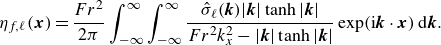 \begin{equation} \eta _{{f},\ell }(\boldsymbol{x}) =\frac {Fr^2}{2\pi }\int _{-\infty }^{\infty }\int _{-\infty }^{\infty }\frac {\hat {\sigma }_{\ell }(\boldsymbol{k})|\boldsymbol{k}|\tanh |\boldsymbol{k}|}{Fr^2k_x^2 - |\boldsymbol{k}|\tanh |\boldsymbol{k}|}\,\mbox{exp}({\mathrm{i}\boldsymbol{k}\cdot \boldsymbol{x}})\,\mbox{d}\boldsymbol{k}. \end{equation}
The denominator in (4.6) has poles that are responsible for the Kelvin wake pattern far downstream of the obstacle. Unlike the linear fKP analysis in § 3, the poles cannot be written down in a simple-closed form. However, following the same strategy as the fKP analysis in § 4, an obvious choice of $\hat {\sigma }_{\ell }(\boldsymbol{k})$
that eliminates the pole in (4.6) is
$\hat {\sigma }_{\ell }(\boldsymbol{k})$
that eliminates the pole in (4.6) is
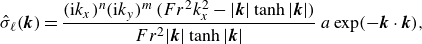 \begin{equation} \hat {\sigma }_{\ell }(\boldsymbol{k}) = \frac {(\mathrm{i}k_x)^n(\mathrm{i}k_y)^m\,(Fr^2k_x^2 - |\boldsymbol{k}|\tanh |\boldsymbol{k}|)}{Fr^2|\boldsymbol{k}|\tanh |\boldsymbol{k}|}\,a\,\mbox{exp}(-\boldsymbol{k}\cdot \boldsymbol{k}), \end{equation}
where $n,m\in \mathbb{N}$
and
$n,m\in \mathbb{N}$
and $a\in \mathbb{R}$
. Imposing (4.7) results in a family of linear wave-free profiles
$a\in \mathbb{R}$
. Imposing (4.7) results in a family of linear wave-free profiles
 \begin{equation} \eta _{{f},\ell }(\boldsymbol{x}) = a\,(\mbox{exp}(-\boldsymbol{x}\cdot\boldsymbol{x}))_{x^{(n)}y^{(m)}}, \end{equation}
where $x^{(n)}$
and
$x^{(n)}$
and $y^{(m)}$
represent the
$y^{(m)}$
represent the $n^{{}}$
th-
$n^{{}}$
th- $x$
and
$x$
and $m^{{}}$
th-
$m^{{}}$
th- $y$
derivatives, respectively. Here, we can choose
$y$
derivatives, respectively. Here, we can choose $n=m=0$
and in this sense the wave-free
$n=m=0$
and in this sense the wave-free $\eta _{{f},\ell }(\boldsymbol{x})$
in the fully nonlinear moving-pressure problem is less restricted than in the fKP system, where
$\eta _{{f},\ell }(\boldsymbol{x})$
in the fully nonlinear moving-pressure problem is less restricted than in the fKP system, where $\eta _{{f},\ell }(\boldsymbol{x})$
has to be a second
$\eta _{{f},\ell }(\boldsymbol{x})$
has to be a second $x$
-derivative of a localised two-dimensional function, see (4.3).
$x$
-derivative of a localised two-dimensional function, see (4.3).
In contrast to the fKP model, where a nonlinear solution can be written down exactly (see (3.2)), we are unable to write down a simple exact nonlinear solution to the moving-pressure problem based on $\eta _{{f},\ell }(\boldsymbol{x})$
and
$\eta _{{f},\ell }(\boldsymbol{x})$
and $\hat {\sigma }_{\ell }(\boldsymbol{k})$
in (4.8) and (4.7), respectively. We could go to higher-order
$\hat {\sigma }_{\ell }(\boldsymbol{k})$
in (4.8) and (4.7), respectively. We could go to higher-order $\alpha$
in (4.5) and choose
$\alpha$
in (4.5) and choose $\hat {\sigma }(\boldsymbol{k})$
at each order judiciously to eliminate the higher-order poles, but the resulting expressions will become increasingly complicated, require inversion of a two-dimensional Fourier integral and it is not at all obvious that the corresponding series solution would be convergent. To avoid this, and inspired by the fact that the nonlinear free surface is identical to the linear free surface in the fKP analysis (see (3.2)), we directly determine
$\hat {\sigma }(\boldsymbol{k})$
at each order judiciously to eliminate the higher-order poles, but the resulting expressions will become increasingly complicated, require inversion of a two-dimensional Fourier integral and it is not at all obvious that the corresponding series solution would be convergent. To avoid this, and inspired by the fact that the nonlinear free surface is identical to the linear free surface in the fKP analysis (see (3.2)), we directly determine $\sigma _{{press}}(\boldsymbol{x})$
by solving the nonlinear moving-pressure problem numerically as a nonlinear inverse problem for
$\sigma _{{press}}(\boldsymbol{x})$
by solving the nonlinear moving-pressure problem numerically as a nonlinear inverse problem for $\sigma _{{press}}(\boldsymbol{x})$
given a prescribed wave-free
$\sigma _{{press}}(\boldsymbol{x})$
given a prescribed wave-free $\eta _{{f}}(\boldsymbol{x})$
, as opposed to the so-called nonlinear forward problem of finding
$\eta _{{f}}(\boldsymbol{x})$
, as opposed to the so-called nonlinear forward problem of finding $\eta _{{f}}(\boldsymbol{x})$
given
$\eta _{{f}}(\boldsymbol{x})$
given $\sigma _{{press}}(\boldsymbol{x})$
.
$\sigma _{{press}}(\boldsymbol{x})$
.
We benchmark our results by choosing two different types of $\eta (\boldsymbol{x})$
from (4.8)
$\eta (\boldsymbol{x})$
from (4.8)
 \begin{equation} \eta _{{f}}(\boldsymbol{x}) = \eta _{{g}}(\boldsymbol{x}) = a\,\mbox{exp}({-\boldsymbol{x}\cdot \boldsymbol{x}}),\quad \eta _{{f}}(\boldsymbol{x}) = \eta _{{s}}(\boldsymbol{x}) = a\,(\mbox{exp}({-\boldsymbol{x}\cdot \boldsymbol{x}}))_{xx}. \end{equation}
The corresponding inversely found $\sigma _{{press}}(\boldsymbol{x})$
are shown in figure 6 for
$\sigma _{{press}}(\boldsymbol{x})$
are shown in figure 6 for $\eta = \eta _{{g}}$
(top two rows) and
$\eta = \eta _{{g}}$
(top two rows) and $\eta = \eta _{{s}}$
(bottom two rows). We make the important observation that these are all localised in space, hence mimicking a finite ‘boat’. As can be seen from the top two rows, corresponding to
$\eta = \eta _{{s}}$
(bottom two rows). We make the important observation that these are all localised in space, hence mimicking a finite ‘boat’. As can be seen from the top two rows, corresponding to $\sigma _{{press}}(\boldsymbol{x})$
when
$\sigma _{{press}}(\boldsymbol{x})$
when $\eta _{{g}}(\boldsymbol{x})$
, for small
$\eta _{{g}}(\boldsymbol{x})$
, for small $Fr$
the forcing term has a single minimum which occurs at the origin, then as
$Fr$
the forcing term has a single minimum which occurs at the origin, then as $Fr$
increases to unity, two distinct minima emerge aligned to the
$Fr$
increases to unity, two distinct minima emerge aligned to the $x$
axis. Increasing
$x$
axis. Increasing $Fr$
further results in the two minima being separated by a maximum. In the bottom row, corresponding to
$Fr$
further results in the two minima being separated by a maximum. In the bottom row, corresponding to $\sigma _{{press}}(\boldsymbol{x})$
when
$\sigma _{{press}}(\boldsymbol{x})$
when $\eta _{{s}}(\boldsymbol{x})$
, the previous description is reversed where instead of maxima there are minima and vice versa. Notice that for large
$\eta _{{s}}(\boldsymbol{x})$
, the previous description is reversed where instead of maxima there are minima and vice versa. Notice that for large $Fr$
the shape of
$Fr$
the shape of $\sigma _{{press}}(\boldsymbol{x})$
for
$\sigma _{{press}}(\boldsymbol{x})$
for $\eta _{{g}} (\boldsymbol{x})$
(top two rows) and
$\eta _{{g}} (\boldsymbol{x})$
(top two rows) and $\eta _{{s}}(\boldsymbol{x})$
(bottom two rows) are similar, except for the opposite sign.
$\eta _{{s}}(\boldsymbol{x})$
(bottom two rows) are similar, except for the opposite sign.
Fully nonlinear moving-pressure problem as $Fr$
is varied. Each panel is plotted in the range
$Fr$
is varied. Each panel is plotted in the range $x\in [-10,10],y\in [-10,10]$
. First and second rows: wave-free profile
$x\in [-10,10],y\in [-10,10]$
. First and second rows: wave-free profile $\eta _{{g}}(\boldsymbol{x})$
and corresponding
$\eta _{{g}}(\boldsymbol{x})$
and corresponding $\sigma _{{press}}(\boldsymbol{x})$
, respectively. Third and fourth rows: wave-free profile
$\sigma _{{press}}(\boldsymbol{x})$
, respectively. Third and fourth rows: wave-free profile $\eta _{{s}}(\boldsymbol{x})$
and corresponding
$\eta _{{s}}(\boldsymbol{x})$
and corresponding $\sigma _{{press}}(\boldsymbol{x})$
, respectively. In both cases
$\sigma _{{press}}(\boldsymbol{x})$
, respectively. In both cases $a=0.01$
(see (4.9)).
$a=0.01$
(see (4.9)).
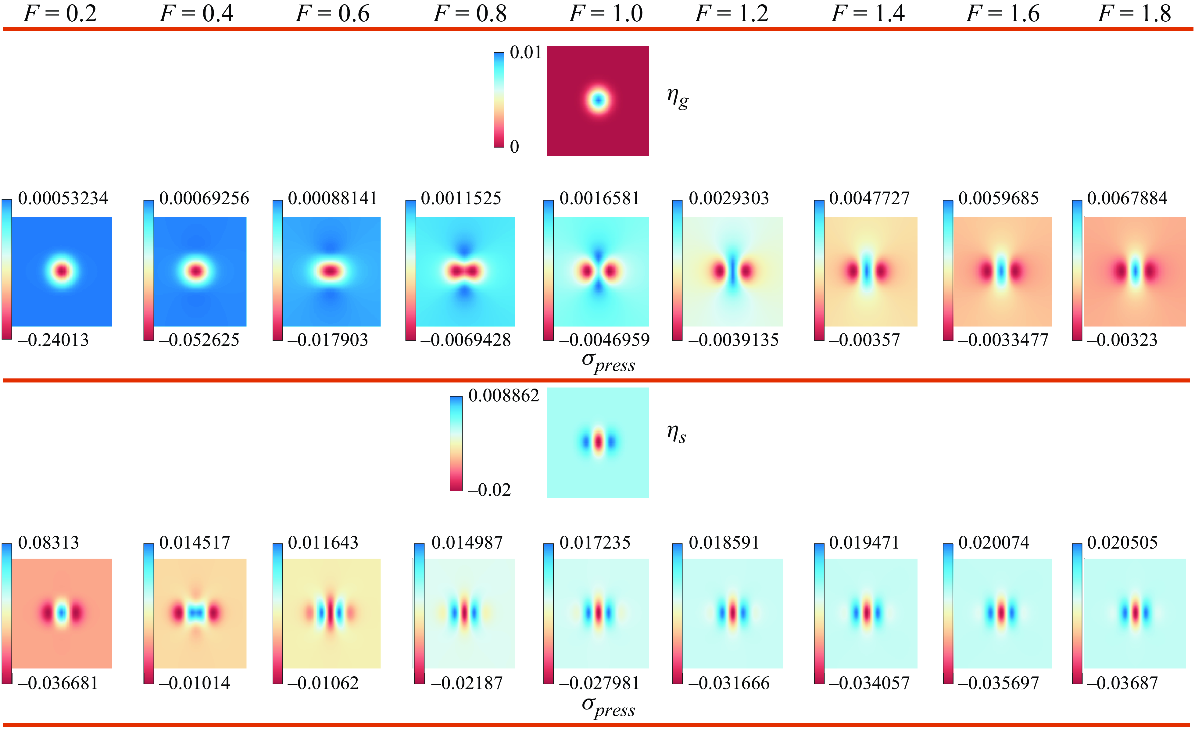
4.4. Topographic-obstacle problem
We now concentrate on the topographic-obstacle problem. Formally, the linear solution to (2.1)–(2.6) in this case is
 \begin{equation} {\eta _{{f},\ell }(\boldsymbol{x}) = \frac {Fr^2}{2\pi }\int _{-\infty }^{\infty }\int _{-\infty }^{\infty }\frac {\hat {\sigma }_{{topog}}(\boldsymbol{k})k_x^2\,\mathrm{sech}\,|\boldsymbol{k}|}{Fr^2k_x^2 - |\boldsymbol{k}|\tanh |\boldsymbol{k}|}\,\mbox{exp}({\mathrm{i}\boldsymbol{k}\cdot \boldsymbol{x}})\,\mbox{d}k_x\mbox{d}k_y.} \end{equation}
An important remark is that the denominator of the integrand in (4.10) is identical to that for the moving-pressure distribution problem in (4.6) and hence the location and strength of the poles in the complex plane are also identical. However, unlike the moving-pressure problem, we would not expect to be able to solve the resulting numerical inverse problem of prescribing the shape of the $z_{{f}}(\boldsymbol{x})$
and then solving (2.1)–(2.6) to find
$z_{{f}}(\boldsymbol{x})$
and then solving (2.1)–(2.6) to find $\sigma _{{topog}}(\boldsymbol{x})$
, as it is likely to be ill posed as it is in the two-dimensional problem (Robbins et al. Reference Robbins, Blyth, Maclean and Binder2023) and sophisticated optimisation techniques, beyond the present scope of this paper, would be expected to be required. We emphasise that, for the moving-pressure problem, there is no numerical evidence that the inverse problem is ill posed.
$\sigma _{{topog}}(\boldsymbol{x})$
, as it is likely to be ill posed as it is in the two-dimensional problem (Robbins et al. Reference Robbins, Blyth, Maclean and Binder2023) and sophisticated optimisation techniques, beyond the present scope of this paper, would be expected to be required. We emphasise that, for the moving-pressure problem, there is no numerical evidence that the inverse problem is ill posed.
However, due to the identical denominator, we can still make progress as the same $\sigma _{\ell }(\boldsymbol{k})$
that eliminates the linear wave pattern in the moving-pressure problem will also eliminate the linear wave pattern in the topographic-obstacle problem. It is not unreasonable to expect, therefore, that choosing
$\sigma _{\ell }(\boldsymbol{k})$
that eliminates the linear wave pattern in the moving-pressure problem will also eliminate the linear wave pattern in the topographic-obstacle problem. It is not unreasonable to expect, therefore, that choosing $\sigma _{{topog}}(\boldsymbol{x}) = \sigma _{{press}}(\boldsymbol{x})$
will result in a significant reduction in the nonlinear wave signature in the forward topographic-obstacle problem. The strategy is as follows. First, we prescribe
$\sigma _{{topog}}(\boldsymbol{x}) = \sigma _{{press}}(\boldsymbol{x})$
will result in a significant reduction in the nonlinear wave signature in the forward topographic-obstacle problem. The strategy is as follows. First, we prescribe $\eta _{{f}}(\boldsymbol{x})$
for the moving-pressure problem and solve the nonlinear inverse problem for
$\eta _{{f}}(\boldsymbol{x})$
for the moving-pressure problem and solve the nonlinear inverse problem for $\sigma _{{press}}(\boldsymbol{x})$
. Next, we set
$\sigma _{{press}}(\boldsymbol{x})$
. Next, we set $\sigma _{{topog}}(\boldsymbol{x})=\sigma _{{press}}(\boldsymbol{x})$
and solve the nonlinear forward topographic-obstacle problem for
$\sigma _{{topog}}(\boldsymbol{x})=\sigma _{{press}}(\boldsymbol{x})$
and solve the nonlinear forward topographic-obstacle problem for $\eta _{{f}}(\boldsymbol{x})$
.
$\eta _{{f}}(\boldsymbol{x})$
.
This process is shown in figure 7 for the specific case of $\eta _{{f}}(\boldsymbol{x}) = \eta _{{g}}(\boldsymbol{x})$
in (4.9). As can be seen in this middle left panel, the wave signature of the nonlinear
$\eta _{{f}}(\boldsymbol{x}) = \eta _{{g}}(\boldsymbol{x})$
in (4.9). As can be seen in this middle left panel, the wave signature of the nonlinear $\eta _{{f}}(\boldsymbol{x})$
for the topographic-obstacle problem is present but barely visible. As a trial case to highlight this minimisation, on the bottom row, we also show
$\eta _{{f}}(\boldsymbol{x})$
for the topographic-obstacle problem is present but barely visible. As a trial case to highlight this minimisation, on the bottom row, we also show $\eta _{{f}}(\boldsymbol{x})$
(bottom-left panel) as a solution to a forwards problem with
$\eta _{{f}}(\boldsymbol{x})$
(bottom-left panel) as a solution to a forwards problem with $\sigma _{{topog}}(\boldsymbol{x}) = \hat {a}\,\mbox{exp}(-\boldsymbol{x}\cdot \boldsymbol{x})$
where
$\sigma _{{topog}}(\boldsymbol{x}) = \hat {a}\,\mbox{exp}(-\boldsymbol{x}\cdot \boldsymbol{x})$
where $\hat {a}$
is chosen so that the integral of
$\hat {a}$
is chosen so that the integral of $\sigma _{{topog}}(\boldsymbol{x})$
over the domain is identical to the integral of the topography in the middle-right panel (value in caption). The comparison between the two resulting
$\sigma _{{topog}}(\boldsymbol{x})$
over the domain is identical to the integral of the topography in the middle-right panel (value in caption). The comparison between the two resulting $\eta _{{f}}(\boldsymbol{x})$
in the middle- and bottom-left panels is striking. These results are for
$\eta _{{f}}(\boldsymbol{x})$
in the middle- and bottom-left panels is striking. These results are for $Fr=1.2$
but similar results exist for
$Fr=1.2$
but similar results exist for $Fr\in [0.2,1.8]$
that we sampled. We leave the highly non-trivial problem of inversely finding a localised topographic obstacle given a prescribed free surface as an open challenge.
$Fr\in [0.2,1.8]$
that we sampled. We leave the highly non-trivial problem of inversely finding a localised topographic obstacle given a prescribed free surface as an open challenge.
Fully nonlinear Euler system when $Fr=1.2$
. Blue box: top left:
$Fr=1.2$
. Blue box: top left: $\eta _{{f}}(\boldsymbol{x})$
for the moving-pressure distribution given by (4.9). Top right: the pressure-distribution,
$\eta _{{f}}(\boldsymbol{x})$
for the moving-pressure distribution given by (4.9). Top right: the pressure-distribution, $\sigma _{{press}}(\boldsymbol{x})$
that results in (4.9) when
$\sigma _{{press}}(\boldsymbol{x})$
that results in (4.9) when $a=0.01$
. Middle right: the prescribed topographic-obstacle
$a=0.01$
. Middle right: the prescribed topographic-obstacle $\sigma _{{topog}}(\boldsymbol{x})=\sigma _{{press}}(\boldsymbol{x})$
. Middle- = left: the resulting free surface for
$\sigma _{{topog}}(\boldsymbol{x})=\sigma _{{press}}(\boldsymbol{x})$
. Middle- = left: the resulting free surface for $\sigma _{{topog}}(\boldsymbol{x})$
. Red box: bottom right: Gaussian topographic obstacle with
$\sigma _{{topog}}(\boldsymbol{x})$
. Red box: bottom right: Gaussian topographic obstacle with $\hat {a} = 0.001653$
chosen so it has identical mass to
$\hat {a} = 0.001653$
chosen so it has identical mass to $\sigma _{{topog}}(\boldsymbol{x})$
. Bottom left: free-surface response for the Gaussian topography.
$\sigma _{{topog}}(\boldsymbol{x})$
. Bottom left: free-surface response for the Gaussian topography.
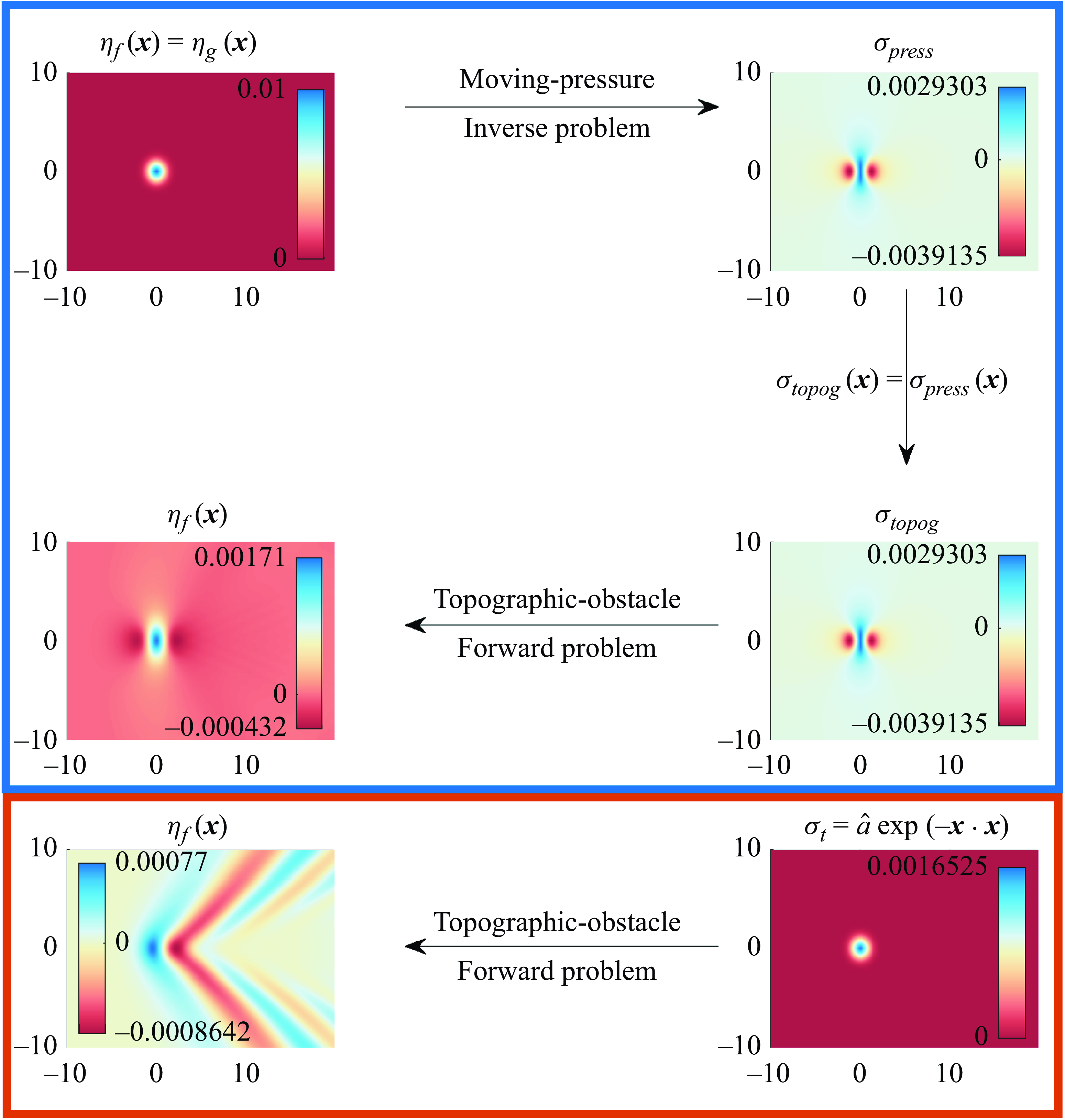
4.5. Wave resistance
It is illuminating to briefly discuss the physical implications of wave-free solutions. To this end, and referring to figure 1, we apply the momentum integral equation for inviscid flow (e.g. Batchelor Reference Batchelor1967) over a control volume confined between the free surface $\Gamma _2$
the bottom
$\Gamma _2$
the bottom $\Gamma _0$
and the four vertical sides
$\Gamma _0$
and the four vertical sides $\Gamma _1$
,
$\Gamma _1$
, $\Gamma _3$
,
$\Gamma _3$
, $\Gamma _4$
and
$\Gamma _4$
and $\Gamma _5$
that are parallel to the
$\Gamma _5$
that are parallel to the $x$
and
$x$
and $y$
axes. Taking the component in the horizontal direction, we obtain
$y$
axes. Taking the component in the horizontal direction, we obtain
 \begin{equation} \mathcal{F} = \iint _{\Gamma _1} (p+\rho u^2) \: {\rm d} S - \iint _{\Gamma _3} (p+\rho u^2) \: {\rm d} S + \iint _{\Gamma _4} v(\rho u) \: {\rm d} S + \iint _{\Gamma _5} (-v)(\rho u) \: {\rm d} S, \end{equation}
where $(u,v)=(\phi _x,\phi _y)$
. The first two terms on the right-hand side represent the flux of total horizontal momentum (e.g. Lighthill Reference Lighthill1978) through the downstream and upstream faces,
$(u,v)=(\phi _x,\phi _y)$
. The first two terms on the right-hand side represent the flux of total horizontal momentum (e.g. Lighthill Reference Lighthill1978) through the downstream and upstream faces, $\Gamma _1$
and
$\Gamma _1$
and $\Gamma _3$
, respectively, and the second two terms on the right-hand side represent the flux of horizontal momentum out of the lateral faces
$\Gamma _3$
, respectively, and the second two terms on the right-hand side represent the flux of horizontal momentum out of the lateral faces $\Gamma _4$
and
$\Gamma _4$
and $\Gamma _5$
. On the left-hand side
$\Gamma _5$
. On the left-hand side
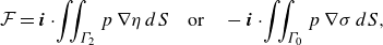 \begin{equation} \mathcal{F} = \boldsymbol{i}\cdot \!\iint _{\Gamma _2} p\,\nabla \eta \, d S \quad \mbox{or} \quad -\boldsymbol{i}\cdot \!\iint _{\Gamma _0} p \, \nabla \sigma \, d S ,\end{equation}
represents either the external pressure force acting on the free surface or the force imposed by the topography on the fluid (or a combination of both). In the former case $\mathcal{F}$
coincides with the wave resistance defined by Havelock (Reference Havelock1917). We interpret (4.11) as meaning that the total external force exerted on the fluid, either by the surface pressure or by the topography, is equal to the net transport of horizontal momentum out through the side faces. In the case of our special topography which localises the surface disturbance, if the control volume is sufficiently large the right-hand side of (4.11) vanishes so that no net momentum is imparted to the surrounding fluid. Then
$\mathcal{F}$
coincides with the wave resistance defined by Havelock (Reference Havelock1917). We interpret (4.11) as meaning that the total external force exerted on the fluid, either by the surface pressure or by the topography, is equal to the net transport of horizontal momentum out through the side faces. In the case of our special topography which localises the surface disturbance, if the control volume is sufficiently large the right-hand side of (4.11) vanishes so that no net momentum is imparted to the surrounding fluid. Then $\mathcal{F}=0$
and the wave resistance is zero, meaning that a ‘boat’ represented by the moving pressure experiences zero wave drag, or the topography exerts a vanishing net force upon the fluid.
$\mathcal{F}=0$
and the wave resistance is zero, meaning that a ‘boat’ represented by the moving pressure experiences zero wave drag, or the topography exerts a vanishing net force upon the fluid.
5. Stability of nonlinear wave-free steady solutions
We now examine the stability of the wave-free steady solutions in the previous section by solving a suite of IVPs. First, we investigate the time-dependent fKP in (2.8) and then the time-dependent fully nonlinear Euler system in (2.1)–(2.6).
5.1. The fKP model equation
We choose the initial condition
 \begin{equation} \eta (\boldsymbol{x},t=0) = 0, \end{equation}
which represents a flat free surface. To benchmark our results, initially, we solve the IVP with a Gaussian forcing function, $\sigma (\boldsymbol{x}) = a\,\mbox{exp}(-\boldsymbol{x}\cdot \boldsymbol{x})$
and a dipole forcing
$\sigma (\boldsymbol{x}) = a\,\mbox{exp}(-\boldsymbol{x}\cdot \boldsymbol{x})$
and a dipole forcing $\sigma (\boldsymbol{x}) = a\,[\mbox{exp}(-\boldsymbol{x}\cdot \boldsymbol{x})]_{xx}$
(
$\sigma (\boldsymbol{x}) = a\,[\mbox{exp}(-\boldsymbol{x}\cdot \boldsymbol{x})]_{xx}$
( $a=0.001$
) and confirm that the weakly nonlinear system evolves towards a steady weakly nonlinear Kelvin wake, see movie_1.mp4 and movie_2.mp4 in the supplementary material.
$a=0.001$
) and confirm that the weakly nonlinear system evolves towards a steady weakly nonlinear Kelvin wake, see movie_1.mp4 and movie_2.mp4 in the supplementary material.


Now, we concentrate on our special form of forcing in (4.4) for the weakly nonlinear fKP model and, to be consistent with the steady results in figure 5, choose $Fr=1.0,a=0.1$
. Figure 8 (corresponding to the animation movie_3.mp4 in the supplementary material) shows the resulting time-dependent behaviour starting from (5.1). As can be seen from the time snapshots, for approximately
$Fr=1.0,a=0.1$
. Figure 8 (corresponding to the animation movie_3.mp4 in the supplementary material) shows the resulting time-dependent behaviour starting from (5.1). As can be seen from the time snapshots, for approximately $0\lt t\lt 7.7$
(top row) a curved wave pattern emerges directly downstream of the forcing. Then, for approximately
$0\lt t\lt 7.7$
(top row) a curved wave pattern emerges directly downstream of the forcing. Then, for approximately $t\geqslant 7.7$
(bottom row) this wake pattern propagates downstream in the form of curved ‘ripples’ before eventually separating and leaving the steady state,
$t\geqslant 7.7$
(bottom row) this wake pattern propagates downstream in the form of curved ‘ripples’ before eventually separating and leaving the steady state, $\eta (\boldsymbol{x},t)$
, which we have confirmed is the steady state in (3.2). This behaviour is generic for a wide range of parameter space (
$\eta (\boldsymbol{x},t)$
, which we have confirmed is the steady state in (3.2). This behaviour is generic for a wide range of parameter space ( $Fr\in [0.2,1.8]$
and
$Fr\in [0.2,1.8]$
and $a\in [-0.1,0.1]$
) and has been thoroughly checked for numerical convergence. Finally, as well as the initial condition in (5.1), numerical simulations provide evidence that the steady state is also stable to two- and three-dimensional perturbations, as shown in movie_4.mp4 and movie_5.mp4. This is strong numerical evidence that the wave-free steady state is not only stable but is also the asymptotic state of the system as
$a\in [-0.1,0.1]$
) and has been thoroughly checked for numerical convergence. Finally, as well as the initial condition in (5.1), numerical simulations provide evidence that the steady state is also stable to two- and three-dimensional perturbations, as shown in movie_4.mp4 and movie_5.mp4. This is strong numerical evidence that the wave-free steady state is not only stable but is also the asymptotic state of the system as $t\to \infty$
. Furthermore, the waves emitted downstream in the initial stage of evolution appear different to the classical Kelvin wake pattern and are similar in nature to the capillary-gravity waves, as shown in Chepelianskii, Chevy & Raphael (Reference Chepelianskii, Chevy and Raphael2008), Closa, Chepelianskii & Raphael (Reference Closa, Chepelianskii and Raphael2010), except these ripple waves only occur downstream. These ripples may be related to the parabolic ‘ripplon’ solutions of the unforced KP equation, as reported in Johnson & Thompson (Reference Johnson and Thompson1978), Nakamura (Reference Nakamura1981), Zhang et al. (Reference Zhang, Yang, Guo and Cao2023, Reference Zhang, Guo and Stepanyants2024) and initial investigations indicate that the ripples we report are indeed parabolic; a detailed analysis of these forced ripple solutions is beyond the scope of this paper and is currently being written up in a separate research paper.
$t\to \infty$
. Furthermore, the waves emitted downstream in the initial stage of evolution appear different to the classical Kelvin wake pattern and are similar in nature to the capillary-gravity waves, as shown in Chepelianskii, Chevy & Raphael (Reference Chepelianskii, Chevy and Raphael2008), Closa, Chepelianskii & Raphael (Reference Closa, Chepelianskii and Raphael2010), except these ripple waves only occur downstream. These ripples may be related to the parabolic ‘ripplon’ solutions of the unforced KP equation, as reported in Johnson & Thompson (Reference Johnson and Thompson1978), Nakamura (Reference Nakamura1981), Zhang et al. (Reference Zhang, Yang, Guo and Cao2023, Reference Zhang, Guo and Stepanyants2024) and initial investigations indicate that the ripples we report are indeed parabolic; a detailed analysis of these forced ripple solutions is beyond the scope of this paper and is currently being written up in a separate research paper.
5.2. Fully nonlinear Euler system
We now investigate the stability of the fully nonlinear Euler steady states for the moving-pressure and topographic-obstacle problems. Concentrating initially on the moving-pressure problem, first, we impose a free surface in (4.9) to obtain the pressure distribution, $\sigma _{{press}}(\boldsymbol{x})$
before setting a flat free surface with a uniform flow as an initial condition
$\sigma _{{press}}(\boldsymbol{x})$
before setting a flat free surface with a uniform flow as an initial condition
 \begin{equation} \eta _{{f}}(\boldsymbol{x},t=0) = 0,\quad \phi (\boldsymbol{x},z,t=0) = x. \end{equation}
We emphasise that $\sigma _{{press}}$
is present at
$\sigma _{{press}}$
is present at $t=0$
. In figure 9 we show that
$t=0$
. In figure 9 we show that $\eta _{{f}}(\boldsymbol{x},t)$
evolves towards the steady wave-free free surface in the moving-pressure problem with forcing in (4.7) for the steady free-surface
$\eta _{{f}}(\boldsymbol{x},t)$
evolves towards the steady wave-free free surface in the moving-pressure problem with forcing in (4.7) for the steady free-surface $\eta _{{g}}(\boldsymbol{x})$
in (4.9). The ripples that get emitted downstream are similar in form to that in the fKP equation but we would expect them to be circular, instead of parabolic, as there is no weak
$\eta _{{g}}(\boldsymbol{x})$
in (4.9). The ripples that get emitted downstream are similar in form to that in the fKP equation but we would expect them to be circular, instead of parabolic, as there is no weak $y$
dependence in the fully nonlinear Euler system.
$y$
dependence in the fully nonlinear Euler system.
For the topographic-obstacle problem we first perform the process described in figure 7 to find $\sigma _{{topog}}(\boldsymbol{x}) = \sigma _{{press}}(\boldsymbol{x})$
using a free surface in (4.9). We then deform the fluid domain using this topographic forcing, set
$\sigma _{{topog}}(\boldsymbol{x}) = \sigma _{{press}}(\boldsymbol{x})$
using a free surface in (4.9). We then deform the fluid domain using this topographic forcing, set $\eta _{{f}}(\boldsymbol{x})=0$
and solve Laplace’s equation in the fluid domain together with (2.2)–(2.6) to obtain an initial condition for
$\eta _{{f}}(\boldsymbol{x})=0$
and solve Laplace’s equation in the fluid domain together with (2.2)–(2.6) to obtain an initial condition for $\phi (\boldsymbol{x},z)$
. Once time is advanced, the subsequent simulations show that the system tends towards the ‘almost’ wave-free steady state, as shown in figure 10.
$\phi (\boldsymbol{x},z)$
. Once time is advanced, the subsequent simulations show that the system tends towards the ‘almost’ wave-free steady state, as shown in figure 10.


Viewed altogether, these calculations show the remarkable stability of the wave-free steady state in both the weakly nonlinear fKP model and fully nonlinear Euler system; our third, and perhaps most significant result of the paper. A carefully constructed forcing term, as described in the previous section, will result in a wave-free profile that can be observed in a physical experiment.
6. Conclusions and perspective
We have demonstrated that the fKP equation is capable of producing the v-shaped Kelvin wave pattern that is observed in practice when an object moves along the surface of water, and we have characterised the associated wedge angle as a function of the Froude number. More importantly, we have shown that, for the fKP and the fully nonlinear Euler system, a judiciously chosen pressure forcing can produce a steady wave-free surface, meaning that the disturbance caused by the forcing is confined to its neighbourhood so that the surface is flat in the far field. In addition, if we use this pressure forcing as a proxy for a topographic obstacle, then the resulting far-field waves in the free-surface profile are significantly diminished. Crucially, using numerical simulations we have demonstrated that the wave-free states are stable in the sense that they are reached as $t\to \infty$
for a suitably posed IVP.
$t\to \infty$
for a suitably posed IVP.
Despite the simplicity of our mathematical argument, this appears to be the first time that wave-free steady solutions have been constructed for the fKP system and their stability properties calculated. Our results provide some evidence that it may be possible to eliminate the Kelvin wake in a real-world setting. However, further work is needed to establish whether wave-free solutions can be observed in a laboratory experiment. On this point, we highlight the work of Chen & Sharma (Reference Chen and Sharma1995) and Chen, Sharma & Stuntz (Reference Chen, Sharma and Stuntz2003) where, using a weakly nonlinear model, similar to the fKP they were able to design a zero wave resistance moving body in a narrow confined channel and these were compared with experiments. Another interesting recent work to highlight is by Euve et al. (Reference Euve, Maurel, Petitjeans and Pagneux2024) in which asymmetric wake patterns have been observed experimentally and whose experimental approach may be relevant for the wave-free solutions in this paper. In addition, it would also be interesting to examine the transverse stability of the two-dimensional solutions discovered in Keeler et al. (Reference Keeler, Binder and Blyth2017, Reference Keeler, Blyth and King2021) at $Fr=1$
, using the computational framework developed here.
$Fr=1$
, using the computational framework developed here.
We emphasise that we have identified wave-free steady states over a large range of the Froude number and forcing amplitude. Regarding wake elimination in real-world applications, our results are at this point only suggestive. Nevertheless, this may ultimately pave the way to improving marine vessel design, including for example the development of ‘stealth’ boats, by reducing the wave drag and minimising the wake signature. It would be interesting to try to perform an experiment using one of our pressure forcings in a flow tuned to the correct Froude number to try to realise our prediction in the laboratory. Our results for topographic obstacles suggest the possibility of designing underwater structures that minimise or eliminate any disruption to the water surface.
For both the fKP model equation and fully nonlinear Euler system studied here, the free-surface profile is extremely sensitive to small changes in the forcing function, as is demonstrated when we use the pressure distribution as a proxy for a topographic obstacle and a downstream Kelvin wake is observed, albeit small of amplitude. Whether a special topographic forcing exists that results in a wave-free surface disturbance in the fully nonlinear Euler system is an open question. The determination of this special topographic forcing will likely require bespoke computational methods to solve the nonlinear inverse problem that arises and we leave this for future work. Finally, it would also be interesting to compare our results with other works that have attempted to minimise the wave drag, including using a ‘pressure-patch model (Tuck & Lazauskas Reference Tuck and Lazauskas2001) and optimisation methods on an actual boat hull (Dambrine & Pierre Reference Dambrine and Pierre2020).
Supplementary movies
Supplementary movies are available at https://doi.org/10.1017/jfm.2025.10225.
Funding
J. S. K acknowledges funding from the Leverhulme Trust; ECF-2021-017.
Declaration of interests
The authors report no conflict of interest.
Data availability statement
The data are available upon request.
Appendix A. Numerical method
The fKP model and the fully nonlinear Euler system are solved in the weak form (as discussed below for each individual system). The common features of the discretisation that apply to both systems are that (i) the equations are discretised using finite elements and the open-source oomph-lib package (Heil & Hazel Reference Heil and Hazel2006), (ii) the test functions, $\psi$
, are piecewise cubic functions and the spatial coordinates and unknown field variables are interpolated using
$\psi$
, are piecewise cubic functions and the spatial coordinates and unknown field variables are interpolated using $\psi$
, (iii) steady states are found using Newton iterations and (iv) time stepping is performed using a backwards Euler order-two method.
$\psi$
, (iii) steady states are found using Newton iterations and (iv) time stepping is performed using a backwards Euler order-two method.
A.1 Weak form of the fKP model
To proceed, (2.8) can be written in conservative form
 \begin{equation} \nabla \cdot \boldsymbol{U} = 0,\quad \boldsymbol{U} = \big[\eta _{t} + (Fr-1)\eta _x - \tfrac{3}{2}\eta \eta _x - \tfrac{1}{6}\eta _{xxx} - \tfrac {1}{2}\sigma _x, -\tfrac {1}{2}\eta _{y}\big]^{\rm T}. \end{equation}
We multiply (A1) by a test function, $\psi$
, multiply over the domain and then use the divergence theorem to obtain the weak residual equation
$\psi$
, multiply over the domain and then use the divergence theorem to obtain the weak residual equation
 \begin{equation} \mathcal{R}_{{fKP}}(\eta )\equiv \iint _{\Omega }\psi \,(\nabla \cdot \boldsymbol{U})\,\mbox{d}V \equiv \int _{\partial \Omega }\psi \,(\boldsymbol{U}\cdot \boldsymbol{n})\,\mbox{d}S -\iint _{\Omega }\nabla \psi \cdot \boldsymbol{U}\,\mbox{d}V= 0. \end{equation}
To discretise and then solve (A2), we truncate the infinite mathematical domain in the range $x\in [-L_x,L_x],y\in [-L_y,L_y]$
and typically we choose
$x\in [-L_x,L_x],y\in [-L_y,L_y]$
and typically we choose $L_x=L_y = 30$
, choose 110 horizontal and vertical elements and choose a time step of
$L_x=L_y = 30$
, choose 110 horizontal and vertical elements and choose a time step of $\Delta t = 0.1$
. On
$\Delta t = 0.1$
. On $y=\pm L_y$
, we set
$y=\pm L_y$
, we set $\boldsymbol{U}\cdot \boldsymbol{n}=\eta _y=0$
and on
$\boldsymbol{U}\cdot \boldsymbol{n}=\eta _y=0$
and on $x=-L_x$
we impose
$x=-L_x$
we impose $\eta =\eta _x=0$
. On
$\eta =\eta _x=0$
. On $x=L_x$
we have to satisfy an unknown radiation condition. For simplicity, and to be consistent with Katsis & Akylas (Reference Katsis and Akylas1987) we set
$x=L_x$
we have to satisfy an unknown radiation condition. For simplicity, and to be consistent with Katsis & Akylas (Reference Katsis and Akylas1987) we set $\eta = 0$
and
$\eta = 0$
and $\boldsymbol{U}\cdot \boldsymbol{n}=0$
on this boundary.
$\boldsymbol{U}\cdot \boldsymbol{n}=0$
on this boundary.
A.2 Weak form of the fully nonlinear Euler system
A full description of this numerical formulation can be found in Keeler & Blyth (Reference Keeler and Blyth2024), where a lot of the details can be carried over to the three-dimensional case we consider here. Briefly summarising, we truncate the infinite mathematical domain in the range $x\in [-L_x,L_x],y\in [-L_y,L_y]$
and typically we choose
$x\in [-L_x,L_x],y\in [-L_y,L_y]$
and typically we choose $L_x=L_y = 20$
. Far upstream and downstream we introduce ‘sponge layers’ so that waves are forced to become locally flat. To obtain the weak formulation, we multiply (2.1) by a test function,
$L_x=L_y = 20$
. Far upstream and downstream we introduce ‘sponge layers’ so that waves are forced to become locally flat. To obtain the weak formulation, we multiply (2.1) by a test function, $\psi (\boldsymbol{x})$
, integrate over the computational domain,
$\psi (\boldsymbol{x})$
, integrate over the computational domain, $\Omega (t)$
, and use the divergence theorem to get our bulk residual
$\Omega (t)$
, and use the divergence theorem to get our bulk residual
 \begin{equation} \mathcal{R}_{{Bulk}}(\boldsymbol{x},\phi (\boldsymbol{x}))\equiv \iint _{\partial \Omega (t)}\left (\boldsymbol{n}\cdot \nabla \phi \right )\psi \,\mbox{d}S-\iiint _{\Omega (t)} \nabla \phi \cdot \nabla \psi \,\mbox{d}V = 0, \end{equation}
where $\partial \Omega (t)$
represents the boundary of
$\partial \Omega (t)$
represents the boundary of $\Omega (t)$
,
$\Omega (t)$
, $\boldsymbol{n}$
is the outwards-pointing unit normal vector on each part of the boundary and
$\boldsymbol{n}$
is the outwards-pointing unit normal vector on each part of the boundary and $\mbox{d}V$
,
$\mbox{d}V$
, $\mbox{d}S$
are differential volume and area elements, respectively. We decompose the boundary into 6 parts;
$\mbox{d}S$
are differential volume and area elements, respectively. We decompose the boundary into 6 parts; $\partial \Omega (t) = \Gamma _0 + \Gamma _1 + \Gamma _2(t) + \Gamma _3 + \Gamma _4 + \Gamma _5$
, see figure 1. The kinematic boundary condition on
$\partial \Omega (t) = \Gamma _0 + \Gamma _1 + \Gamma _2(t) + \Gamma _3 + \Gamma _4 + \Gamma _5$
, see figure 1. The kinematic boundary condition on $\Gamma _2$
(2.2), uniform-flow condition on
$\Gamma _2$
(2.2), uniform-flow condition on $\Gamma _1$
(2.5) and no-penetration condition (2.6), can be incorporated directly into (A3). As there is a ‘sponge layer’ near the boundaries at
$\Gamma _1$
(2.5) and no-penetration condition (2.6), can be incorporated directly into (A3). As there is a ‘sponge layer’ near the boundaries at $\Gamma _4$
and
$\Gamma _4$
and $\Gamma _5$
we impose
$\Gamma _5$
we impose $\boldsymbol{n}\cdot \nabla \phi =0$
on these lateral boundaries which can also be incorporated as a natural boundary condition in (A3). Finally, we impose the uniform-flow condition on
$\boldsymbol{n}\cdot \nabla \phi =0$
on these lateral boundaries which can also be incorporated as a natural boundary condition in (A3). Finally, we impose the uniform-flow condition on $\Gamma _3$
as an essential boundary condition by setting
$\Gamma _3$
as an essential boundary condition by setting $\phi = -L$
on
$\phi = -L$
on $\Gamma _3$
.
$\Gamma _3$
.
To satisfy (2.3) we multiply by a test function and integrate over the free surface to obtain
 \begin{equation} \mathcal{R}_{{Dyn}}(\boldsymbol{x},\phi (\boldsymbol{x}))\equiv \iint _{z = z_{{f}}(\boldsymbol{x},t)}\left (\phi _t + \frac {1}{2}|\nabla \phi |^2 + \frac {1}{Fr^2}z_{{f}} +\sigma _{{press}} - \frac {1}{2}-\frac {1}{Fr^2}\right )\psi \,\mbox{d}S = 0. \end{equation}
For the forward problem, the steady forms of (A3) and (A4) are solved to determine the free-surface location, $z_{{f}}(\boldsymbol{x},t)$
, and the velocity potential in the fluid,
$z_{{f}}(\boldsymbol{x},t)$
, and the velocity potential in the fluid, $\phi (\boldsymbol{x},t)$
with a prescribed forcing whilst for the inverse problem we solve for
$\phi (\boldsymbol{x},t)$
with a prescribed forcing whilst for the inverse problem we solve for $\sigma _{{press}}(\boldsymbol{x})$
given a prescribed
$\sigma _{{press}}(\boldsymbol{x})$
given a prescribed $z_{{f}}(\boldsymbol{x})$
.
$z_{{f}}(\boldsymbol{x})$
.
We typically chose 70 $\times$
40
$\times$
40 $\times$
2 elements in the
$\times$
2 elements in the $x\times y\times z$
directions and chose a time step
$x\times y\times z$
directions and chose a time step $\Delta t = 1.0$
. To account for the unknown free surface,
$\Delta t = 1.0$
. To account for the unknown free surface, $\eta (\boldsymbol{x},t)$
, we use a structured brick mesh with a spine-node update strategy. An important remark is that despite calculating quantities in the bulk fluid as well as the free surface, the corresponding Jacobian matrix is sparse, in contrast to the Green’s function approaches. We have not used any Newton–Krylov methods, nor applied pre-conditioning, the use of which would result in significant computational speed-up and we leave this as an open challenge.
$\eta (\boldsymbol{x},t)$
, we use a structured brick mesh with a spine-node update strategy. An important remark is that despite calculating quantities in the bulk fluid as well as the free surface, the corresponding Jacobian matrix is sparse, in contrast to the Green’s function approaches. We have not used any Newton–Krylov methods, nor applied pre-conditioning, the use of which would result in significant computational speed-up and we leave this as an open challenge.


 Open access