


1. Introduction
Within decision theory, one major distinction is between theories or models with only risk, and those with ambiguity. These models are distinguished according to whether agents always have a unique probability distribution over all decision-relevant events (risky models/agents), or not (ambiguous models/agents). Imagine, for example, an agent trying to decide whether to hand money over to another agent, and therefore estimating the probability that the other agent would in turn hand over the goods. Perhaps it is the agent’s first black market transaction, so that the agent does not know how likely a successful transaction really is; they don’t have prior experience to base their expectations on, and nobody is collecting and publishing statistics. An ambiguous agent does not reduce her belief to a single probability distribution over the events and may for instance believe that the success probability is between 0.5 and 0.9, while a risky (or non-ambiguous) agent instead always believes that the success probability is precisely 0.7, or precisely 0.8759, or similar. This paper addresses the long-standing but still unsettled question of the status of ambiguous beliefs. Are agents with such beliefs rational? Do they get better or worse results? Specifically, we address the question of whether non-ambiguous beliefs are better in an evolutionary sense: would a process of natural selection in a competitive environment prefer agents with non-ambiguous beliefs, hence eliminating ambiguous agents from the population?
Ambiguity is an important phenomenon. First and foremost, people regularly face situations in which probabilities are not given. Furthermore, the empirical evidence makes clear that real people typically reveal ambiguous beliefs in some kinds of situations (Ellsberg, Reference Ellsberg1961; Trautmann and van de Kuilen, Reference Trautmann, van de Kuilen, Keren and Wu2016). This means that the ambiguous beliefs affect people’s behaviour; for example, if our agent contemplating their black market transaction is ambiguity averse, this may lead them to go home rather than to hand over their money, even in cases where a counterpart who did not perceive or did not dislike ambiguity would have gone ahead with the transaction. For this reason, economists have been studying ambiguity empirically, developing theoretical models of decision under ambiguity, and incorporating ambiguity into analyses of economic phenomena more and more over the past decades (see Etner et al. (Reference Etner, Jeleva and Tallon2012) for a survey). In short, ambiguity is important to economists primarily because it in fact greatly influences people’s decisions.
Philosophers too have increasingly incorporated ambiguity into their research, typically focusing on the question of whether rationality permits or even requires agents to have ambiguous beliefs and to be sensitive to ambiguity. The key intuition behind the rationality of ambiguous beliefs is that ambiguous beliefs best reflect the agent’s evidence in many if not most situations (see e.g. Joyce Reference Joyce2005; Gilboa et al. Reference Gilboa, Postlewaite and Schmeidler2009; Joyce Reference Joyce2010; Gilboa Reference Gilboa2015; pace Carr Reference Carr2020). Suppose, for example, that I have asked two friends how reliably my intended exchange partner hands over the goods when I hand over the money, and one friend says “fifty-fifty” while the other says “90%”. Suppose that the two friends have otherwise similar and lengthy experience with these transactions, and that it isn’t clear why one has a better success rate than the other. I therefore also can’t judge whether the exchange partner is going to treat me like the 50% friend (maybe because we have the same gender), the 90% friend (we are part of the same ethnic group), or in some other way. In such a case, the argument goes, it makes sense for my belief to reflect the range of success probabilities, and not necessarily its midpoint or any other point between the two.
However, the normative status of ambiguous beliefs remains controversial within philosophy. For example, one argument against the rationality of ambiguous beliefs comes from epistemic utility theory; ambiguous beliefs have been shown not to maximize expected accuracy in that framework, given the assumptions usually made by epistemic utility theorists (Schoenfield Reference Schoenfield2017; Berger and Das Reference Berger and Das2020; see also Seidenfeld et al. Reference Seidenfeld, Schervish and Kadane2012; Mayo-Wilson and Wheeler Reference Mayo-Wilson and Wheeler2016). It has been shown, however, that different assumptions about epistemic value can yield different verdicts about ambiguous beliefs (Konek Reference Konek2019). The economics literature discusses another important concern, namely that agents with ambiguous beliefs are subject to dynamic inconsistency (Epstein and Le Breton Reference Epstein and Le Breton1993; Ghirardato Reference Ghirardato2002; Al-Najjar and Weinstein Reference Al-Najjar and Weinstein2009). Further research has qualified this claim, though, for example by specifying conditions under which dynamic inconsistency cannot arise or even questioning the interpretation of the purported examples in which it does arise (see e.g. Epstein and Schneider Reference Epstein and Schneider2007; Hill Reference Hill2020).
Even if we set aside these normative debates, our understanding of ambiguity is in an important respect partial, and in a respect that both economists and philosophers should care about. To understand the deficit, consider that there are two main general approaches to rationality, which we will refer to as classical rationality and ecological rationality (cf. Rich Reference Rich2016). Both philosophy and economics have expended significant effort, and made significant progress, in investigating the classical rationality of ambiguous beliefs and ambiguity sensitivity. This includes the development of axiomatic theories of ambiguity sensitive behaviour, which represent the agents as having coherent preferences (for early examples, see Schmeidler Reference Schmeidler1989; Gilboa and Schmeidler Reference Gilboa and Schmeidler1989); the formulation of abstract rules of rationality, such as to respect one’s evidence, to choose consistently over time, or to maximize expected belief accuracy (as discussed above); and Dutch Book arguments, which address the theoretical possibility of being subjected to a sure loss (Diecidue and Wakker Reference Diecidue and Wakker2002; Bradley Reference Bradley2012; Coletti et al. Reference Coletti, Petturiti and Vantaggi2019). The ecological rationality of ambiguity, however, is not well understood.
Ecological rationality is fundamentally about the (expected) success of the agent’s decisions or reasoning, given their environment (see e.g. Gigerenzer Reference Gigerenzer2000; Gigerenzer et al. Reference Gigerenzer, Hertwig and Pachur2011). As Simon (Reference Simon1990) famously wrote, “[h]uman rational behavior … is shaped by a scissors whose two blades are the structure of task environments and the computational capabilities of the actor.” In contrast to classical rationality, ecological rationality does not depend on whether the agent shows coherence, but rather on whether any incoherence carries actual costs (Arkes et al. Reference Arkes, Gigerenzer and Hertwig2016); it does not depend on whether an agent could be exposed to a sure loss in principle, but on whether they are actually expected to lose or gain as a result of their choices, which is a separate question (Berg et al. Reference Berg, Eckel and Johnson2008, Reference Berg, Biele and Gigerenzer2016; Rich Reference Rich2018b). Since economists are ultimately interested in actual economic choices and their impact, the real world consequences of ambiguous beliefs should clearly matter a lot; this is also evident in the large economic literature on ambiguity which focuses on modelling it, measuring it, and understanding its consequences, and not on deciding questions of ultimate normative rationality. For philosophers, the ecological rationality of ambiguous beliefs matters for two reasons. First, philosophers have a strong direct interest in making normative judgements, and when it comes to rationality, classical rationality simply doesn’t tell the whole story. Philosophers (should) care about rationality for real people in the real world and not just about idealized beings in a hypothetical world, and this means evaluating ecological rationality too. Second, philosophers’ judgements about rational beliefs and decisions feed into further research where these judgements serve as an input. For example, philosophers often assume rational agents to be expected utility maximizers (and hence, not ambiguity sensitive), but different assumptions about rationality can yield different downstream conclusions (see e.g. Rich Reference Rich2021). Hence, answering basic questions about whether agents’ responses to ambiguity are likely to help or to harm them is of broad, cross-disciplinary value.
In this paper, we explore a way in which ambiguity can be conducive to ecological rationality, by improving outcomes in contexts which are especially important for humans. Our starting point is new analyses of ambiguity in social and strategic contexts. These arguments go beyond appeals to intuition or principles and show that in some cases agents can be better off from a utility perspective when ambiguity is enabled. Not only can agents benefit by keeping others uncertain of their own strategies (Greenberg Reference Greenberg2000), but better outcomes for all can become possible with the introduction of ambiguity (Binmore Reference Binmore2009; Jamison and Karlan Reference Jamison and Karlan2009; Riedel and Sass Reference Riedel and Sass2014; De Castro and Yannelis Reference De Castro and Yannelis2018). In particular, it has been shown that ambiguity can help or improve coordination (Eichberger et al. Reference Eichberger, Kelsey and Schipper2009; Agranov and Schotter Reference Agranov and Schotter2012) and cooperation (Riedel and Sass Reference Riedel and Sass2014; Eichberger et al. Reference Eichberger, Grant and Kelsey2018) in some kinds of games. Hence, in evaluating agents with ambiguous beliefs, it is important to look beyond the individualist context and consider benefits to ambiguous beliefs that only arise in multi-agent settings.
Ecological rationality does not deem a decision or reasoning strategy to be flat-out rational or irrational, neither on the basis of abstract arguments (like classical rationality) nor on the basis of isolated examples like those appearing in the papers above. Instead, an ecological rationality judgement is always comparative (relative to alternative cognitive strategies) and contextual (relative to a specified environment) (Rich Reference Rich2018a). This means that to robustly assess the ecological rationality of ambiguous beliefs, for example, we need to measure the performance of agents with ambiguous beliefs against the performance of agents with salient alternative beliefs, relative to a clearly specified, ecologically important, and reasonably broad environment – such as coordination games. In this way, we can form a general picture of how well the ambiguous agents can be expected to do in the environment in question. Our evolutionary modelling approach allows us to do this – it allows us to study salient classes of choice problems and to track the relative performance of different cognitive strategies (most importantly, both ambiguous and non-ambiguous ones). It also, of course, provides understanding of what cognitive strategies would be favoured by natural selection in the given environments, and can therefore contribute to explanations of humans’ observed responses to ambiguity.
This paper therefore uses evolutionary simulation models to study the consequences of natural selection for ambiguous and non-ambiguous agent types in a varied strategic environment, similar to the one in Galeazzi and Franke (Reference Galeazzi and Franke2017) and Galeazzi and Galeazzi (Reference Galeazzi and Galeazzi2021). Relatedly, Eichberger and Guerdjikova (Reference Eichberger and Guerdjikova2018) and Schipper (Reference Schipper2021) study optimism and pessimism (opposing ambiguity attitudes) using evolutionary models; the former use the replicator dynamics, while the latter look at evolutionary stability. Here we use agent-based models and we focus on the contrasts between non-strategic, strategic and coordination problems (due to the intuition that ambiguity helps agents to coordinate).Footnote 1 We affirm the previous finding that ambiguous agents can survive evolution, and additionally show that ambiguous agents do better in strategic situations than in single-agent choice problems, and in particular can do far better than expected-utility agents when coordination is rewarded. This fits well with the examples in the literature in which ambiguity helps agents to coordinate, and supports the hypothesis that this is a fairly general phenomenon rather than a feature of the particular games which have been studied.
The remainder of this paper is organized as follows: section 2 explains the models we use, in particular the (ambiguous and non-ambiguous) strategies present in the population and the environment in which the agents interact. Sections 3, 4 and 5 present the results of our simulations for single-agent decision problems, generic games and coordination games, respectively. Section 6 then presents results for a specific kind of coordination game inspired by the literature on linguistic ambiguity. Section 7 concludes.
2. The Model
2.1 Agent Types
The population includes agents of different types, where the types are characterized by different ways of selecting actions. There are four classic decision criteria that we consider here: maxmin expected utility, expected utility maximization, realization-regret minimization and distribution-regret minimization. Arguably, this list includes some of the most important decision criteria in the literature. The expected utility maximizer is the most important type in decision theory and economics in general (von Neumann and Morgenstern Reference von Neumann and Morgenstern1944; Savage Reference Savage1954). The maxmin criterion has been extremely relevant in decision theory and statistics (von Neumann and Morgenstern Reference von Neumann and Morgenstern1944; Wald Reference Wald1945, Reference Wald1950; Gilboa and Schmeidler Reference Gilboa and Schmeidler1989), while regret minimization has also been advanced as an empirically supported variant (Loomes and Sugden Reference Loomes and Sugden1982) and even named ‘a bold alternative to the alternatives’ (Bleichrodt and Wakker Reference Bleichrodt and Wakker2015).
Two other criteria, a random type and an altruistic type, are added to the population on top of the classic four above in order to have more diversity in the population, and in the case of the random type also as a control. Of these types, expected utility maximization and its altruistic variant are non-ambiguous, as they have probabilistic, non-ambiguous beliefs; maxmin and realization- and distribution-regret minimization are ambiguous types, since they use sets of probabilities as their beliefs. Since the random type does not use any beliefs, they fall into neither category. All these criteria are formally defined below.
In general, a decision criterion can be defined as a function
 $${\rm{Decision\;Criterion}}{:}\ {\rm{Utilities}} \times {\rm{Beliefs}} \to {\rm{Actions}}$$
which associates a utility and a belief with an action choice in a decision problem $\left( {S,A,Z,f} \right)$
where
$\left( {S,A,Z,f} \right)$
where $S$
is the set (which we can assume to be finite for our current purposes) of possible states of the world,
$S$
is the set (which we can assume to be finite for our current purposes) of possible states of the world, $A$
is the set of actions of the decision maker,
$A$
is the set of actions of the decision maker, $Z$
is the set of outcomes and
$Z$
is the set of outcomes and $f$
is the outcome function
$f$
is the outcome function
 $$f{:}\ S \times A \to Z.$$
In decision theory, utilities $u$
are usually represented by a function
$u$
are usually represented by a function
 $$u{:}\ Z \to {\mathbb R}$$
and beliefs $B$
can be represented in different ways, such as a set of states
$B$
can be represented in different ways, such as a set of states $B \subseteq S$
, a probability distribution
$B \subseteq S$
, a probability distribution $B \in {\rm{\Delta }}\left( S \right)$
over the states, or a set of probability distributions
$B \in {\rm{\Delta }}\left( S \right)$
over the states, or a set of probability distributions $B \subseteq {\rm{\Delta }}\left( S \right)$
. Here we adopt the last representation, to allow agents to have ambiguous beliefs.
$B \subseteq {\rm{\Delta }}\left( S \right)$
. Here we adopt the last representation, to allow agents to have ambiguous beliefs.
The criteria used within the population can then be defined as follows. Expected utility maximization, axiomatized by Savage (Reference Savage1954), implies that the belief set $B$
is a single probability measure
$B$
is a single probability measure $p \in {\rm{\Delta }}\left( S \right)$
, and it selects an action
$p \in {\rm{\Delta }}\left( S \right)$
, and it selects an action ${a^{\rm{*}}}$
that maximizes the expected utility:
${a^{\rm{*}}}$
that maximizes the expected utility:
 $${a^{\rm{*}}} \in {\rm{argma}}{{\rm{x}}_{a \in A}}{E_p}[u|a]$$
where
 $${E_p}[u|a] = \mathop \sum \limits_{s \in S} u\left( {f\left( {s,a} \right)} \right)p\left( s \right).$$
Maxmin expected utility, axiomatized by Gilboa and Schmeidler (Reference Gilboa and Schmeidler1989), prescribes picking an action ${a^{\rm{*}}}$
that maximizes the minimum expected utility given the belief set
${a^{\rm{*}}}$
that maximizes the minimum expected utility given the belief set $B$
$B$
 $${a^{\rm{*}}} \in {\rm{argma}}{{\rm{x}}_{a \in A}}\mathop {{\rm{min}}}\limits_{p \in B} {E_p}[u|a].$$
Realization-regret minimization is the version of regret minimization that has gained the most attention in decision theory through the axiomatizations in Hayashi (Reference Hayashi2008) and Stoye (Reference Stoye2011). Given a probability measure $p \in {\rm{\Delta }}\left( S \right)$
, the realization-regret of an action
$p \in {\rm{\Delta }}\left( S \right)$
, the realization-regret of an action $a \in A$
is defined by
$a \in A$
is defined by
 $$\begin{align}{r_R}\left( {a,p} \right): &= {E_p}\left[ {\mathop {{\rm{max}}}\limits_{a{\rm{'}} \in A} u\left( {f\left( {s,a{\rm{'}}} \right)} \right) - u\left( {f\left( {s,a} \right)} \right)} \right] \\&= \mathop \sum \limits_{s \in S} p\left( s \right)\left( {\mathop {{\rm{max}}}\limits_{{\rm{'}} \in A} u\left( {f\left( {s,a{\rm{'}}} \right)} \right) - u\left( {f\left( {s,a} \right)} \right)} \right)\end{align}$$
and realization-regret minimization picks an action ${a^{\rm{*}}}$
that minimizes the maximum realization-regret:
${a^{\rm{*}}}$
that minimizes the maximum realization-regret:
 $${a^{\rm{*}}} \in {\rm{argmi}}{{\rm{n}}_{a \in A}}\mathop {{\rm{max}}}\limits_{p \in B} {r_R}\left( {a,p} \right).$$
Distribution-regret minimization follows the same logic as realization-regret minimization, in that it dictates choosing an action ${a^{\rm{*}}}$
that minimizes the maximum distribution-regret:
${a^{\rm{*}}}$
that minimizes the maximum distribution-regret:
 $${a^{\rm{*}}} \in {\rm{argmi}}{{\rm{n}}_{a \in A}}\mathop {{\rm{max}}}\limits_{p \in B} {r_D}\left( {a,p} \right)$$
where the distribution-regret of an action $a$
given probability measure
$a$
given probability measure $p$
is defined as
$p$
is defined as
 $${r_D}\left( {a,p} \right): = \mathop {{\rm{max}}}\limits_{a{\rm{'}} \in A} {E_p}\left[ {u|a{\rm{'}}} \right] - {E_p}[u|a] = \mathop {{\rm{max}}}\limits_{a{\rm{'}} \in A} \mathop \sum \limits_{s \in S} p\left( s \right)u\left( {f\left( {s,a{\rm{'}}} \right)} \right) - \mathop \sum \limits_{s \in S} p\left( s \right)u\left( {f\left( {s,a} \right)} \right).$$
The altruistic type acts according to a criterion based on the altruistic utility function ${u_{alt}}$
, which essentially pertains to game-theoretic situations. A game is just an interactive decision problem, where multiple agents have to take actions and the outcome depends on the actions of all the agents involved. In parallel to the definition of a decision problem above, we can formally define a game as a tuple
${u_{alt}}$
, which essentially pertains to game-theoretic situations. A game is just an interactive decision problem, where multiple agents have to take actions and the outcome depends on the actions of all the agents involved. In parallel to the definition of a decision problem above, we can formally define a game as a tuple $(J,( {{A_j}{)_{j \in J}},Z,f} )$
where
$(J,( {{A_j}{)_{j \in J}},Z,f} )$
where $J$
is the set of agents,
$J$
is the set of agents, ${A_j}$
is the set of actions of agent
${A_j}$
is the set of actions of agent $j \in J$
,
$j \in J$
, $Z$
is the set of outcomes and
$Z$
is the set of outcomes and $f:{ \times\!\!_{j \in J}}\ {A_j} \to Z$
is the outcome function. Given a game and utility
$f:{ \times\!\!_{j \in J}}\ {A_j} \to Z$
is the outcome function. Given a game and utility
 $${u_j}:Z \to {\mathbb R}$$
for each agent $j \in J$
, the altruistic utility function is then defined as
$j \in J$
, the altruistic utility function is then defined as
 $${u_{alt}}\left( z \right) = \mathop \sum \limits_{j \in J} {u_j}\left( z \right).$$
The altruistic decision criterion is then defined as the maximization of expected utility, except for the use of the altruistic utility ${u_{alt}}$
in place of the utility
${u_{alt}}$
in place of the utility $u$
, i.e. the altruistic criterion selects an action that maximizes expected altruistic utility:
$u$
, i.e. the altruistic criterion selects an action that maximizes expected altruistic utility:
 $${a^{\rm{*}}} \in {\rm{argma}}{{\rm{x}}_{a \in A}}{E_p}[{u_{alt}}|a].$$
The evolution of altruism has been studied at least since Hamilton (Reference Hamilton1964); see Okasha (Reference Okasha2018: Ch. 5) for discussion. Finally, the random type just picks an action uniformly at random.
2.2 The Environment
In the following, we study the evolution of ambiguous beliefs using agent-based modelling (ABM) and a multigame framework. In the multigame environment, different (possibly interactive) decision problems are generated (by randomly drawing values from an interval) and placed on a $k \times k$
toroidal grid.Footnote
2
It is valuable to study decision-making in this framework because it allows us to represent a variety of decision problems, which better matches real-world decision-making than would a model without this variety. In the Appendix, we also abstract away from any spatial component by moving to the setting of evolutionary game theory.
$k \times k$
toroidal grid.Footnote
2
It is valuable to study decision-making in this framework because it allows us to represent a variety of decision problems, which better matches real-world decision-making than would a model without this variety. In the Appendix, we also abstract away from any spatial component by moving to the setting of evolutionary game theory.
The payoffs for these decision problems represent fitness (in the biological sense), and for everything that follows, we fix the agents’ subjective utility (the function u above) as their fitness. The only exception to this is the altruistic type, for whom their utility is the sum of their and their opponent’s fitness. We then generate a population of agents and randomly place them on the grid. The grid is hence the agents’ environment, or playground. For all simulations reported here, half of the cells are populated by agents and the other half are unoccupied. We allow only one agent per cell.
At the beginning of the first generation, the decision criteria are randomly distributed to the agents in equal proportions, so that no criterion is over- or under-represented in the first generation. We know from section 2.1 that for a decision criterion such as those considered here to produce a choice two things are needed: utilities attached to outcomes, and beliefs attached to the opponent’s actions in game environments, or to the possible states of the world in single-agent decision environments. While the utilities are already given by the fitness payoffs of the decision matrix, each decision problem on the grid is also paired with a belief set $B$
. For our purposes,
$B$
. For our purposes, $B$
is then a random convex subset of the simplex (i.e. the set of all probability distributions over the states of the world in single-agent decisions and the other agent’s actions in interactive decisions). This set B is enough to fully represent the beliefs of the ambiguous types, and to determine their choices. In our black market example above, B would represent the set of probability distributions over successful and unsuccessful transactions that are compatible with whatever evidence the agent has gathered, i.e. the set of probability distributions assigning probability 0.5–0.9 to a successful transaction. For each of the non-ambiguous agents (i.e. the expected utility maximizers and the altruistic agents), we set her belief to be a single probability distribution drawn at random from
$B$
is then a random convex subset of the simplex (i.e. the set of all probability distributions over the states of the world in single-agent decisions and the other agent’s actions in interactive decisions). This set B is enough to fully represent the beliefs of the ambiguous types, and to determine their choices. In our black market example above, B would represent the set of probability distributions over successful and unsuccessful transactions that are compatible with whatever evidence the agent has gathered, i.e. the set of probability distributions assigning probability 0.5–0.9 to a successful transaction. For each of the non-ambiguous agents (i.e. the expected utility maximizers and the altruistic agents), we set her belief to be a single probability distribution drawn at random from $B$
.Footnote
3
$B$
.Footnote
3
Each cell of the grid thus comes with two things: a (possibly interactive) decision problem and a set $B$
of probability distributions over the domain of uncertainty (see Figure 1). Note that this modelling choice entails two features: First, for any given decision problem, all the agents have the same belief set
$B$
of probability distributions over the domain of uncertainty (see Figure 1). Note that this modelling choice entails two features: First, for any given decision problem, all the agents have the same belief set $B$
. Ambiguous agents therefore all have the same belief; probabilistic agents will generally have different specific beliefs,Footnote
4
but these will be all included in
$B$
. Ambiguous agents therefore all have the same belief; probabilistic agents will generally have different specific beliefs,Footnote
4
but these will be all included in $B$
. Second, in the interactive case, there are no requirements about the belief in the rationality of the opponent. A few words about these two features are in order. The rationale behind the first feature is that we want to focus on the main qualitative distinction between ambiguous and probabilistic beliefs without making any further assumption about the beliefs of probabilistic agents other than that they are probabilistic and included in
$B$
. Second, in the interactive case, there are no requirements about the belief in the rationality of the opponent. A few words about these two features are in order. The rationale behind the first feature is that we want to focus on the main qualitative distinction between ambiguous and probabilistic beliefs without making any further assumption about the beliefs of probabilistic agents other than that they are probabilistic and included in $B$
. The second comes from the fact that the approach of the present work is ecological and evolutionary more than strategic. No restrictions about agents’ beliefs in the rationality of other agents are therefore imposed. However also notice that, as the decision criteria considered here are all somehow “rational”, no agent – except for the random type of course – ever chooses an irrational (dominated) action.
$B$
. The second comes from the fact that the approach of the present work is ecological and evolutionary more than strategic. No restrictions about agents’ beliefs in the rationality of other agents are therefore imposed. However also notice that, as the decision criteria considered here are all somehow “rational”, no agent – except for the random type of course – ever chooses an irrational (dominated) action.
Multigame environments with interactive (1a) and single-agent (1b) decisions. Each grid cell is associated with both a decision matrix and a belief set. The dots on the grid represent the agents, the different dot colours represent the different agent types (i.e. the agents’ decision criteria), the grey areas in the simplexes shown to the side represent the belief sets associated with each decision. Notice that those grids have to be thought of as being toroidal.

After the environment is created and the agents are placed on the grid, decisions are made. For single-agent decisions, agents react to the decision problem on their own cell. In interactive decision problems, agents interact with their neighbours. Specifically, when two agents are in two adjacentFootnote 5 cells, they play together the two games corresponding to the cells they are in. In all cases, the obtained payoffs from the decisions are recorded. After all decisions have been made, all agents move by one cell either horizontally or vertically at random into an unoccupied cell, and the round ends. This procedure is repeated anew in each subsequent round. The spatial aspect of the environment and the fact that agents move randomly do not play a substantial role, but instead just provide a convenient way to have multiple games in the environment. The Appendix shows that we get essentially the same results if we abstract away from the spatial component by using the evolutionary game theory methodology of just calculating expected payoffs for the types in the population.
After a number of rounds, a generation ends and the agents in the population reproduce in the following way. A percentage of the worst-performing agents dies, and those who die are replaced by new agents. New agents are created by drawing criteria at random proportional to the accumulated fitness of the types in the previous generation. Specifically, the probability that a new agent is of a given type t is equal to the total accumulated payoff of that type, divided by the total accumulated payoffs in the population. This means that two factors matter to the population composition in the next generation: how well the individuals of each type performed, and how common the type was in the population. Note that our rule for the evolution of the population is simply the translation into agent-based modelling of the rule for population change given by the replicator dynamics in standard evolutionary game theory. The key difference is that our rule uses the actual accumulated fitness since we model individual agents, whereas the replicator dynamics – which only represents proportions of types in the population and not individuals – uses expected fitness. However, given the size of the environment, we expect the actual accumulated fitness to approximate the expected fitness. That this is the case is confirmed by the evolutionary game theory results in the Appendix, which show that using the replicator dynamics directly yields very similar results.
The qualification of the concept of environment is important to understand the difference between our approach here and that of classic evolutionary game theory. In classic evolutionary game theory, the environment consists of two fundamental elements: the population of agents and the game played by the agents that drives the evolution of the population. Each agent type then represents a possible action that can be played in the game. In our case instead, the environment consists of the population of agents and a set of different games that are played by the agents and drive the evolution. The agent types in our model then represent various possible decision criteria.
To exemplify, consider an environment consisting of a population with two types of decision criteria, maxmin expected utility and regret minimization; and of the following three games. The first game is a Stag Hunt, the second is a Prisoner’s Dilemma, and the third is an anti-coordination game. For simplicity, let the associated beliefs represent full uncertainty, i.e. $B = {\rm{\Delta }}\left( {\left\{ {I,II} \right\}} \right)$
, for each of the three games.
$B = {\rm{\Delta }}\left( {\left\{ {I,II} \right\}} \right)$
, for each of the three games.

When faced with the Stag Hunt, the maximinimizers want to maximize the minimum outcome and thus choose action $II$
, because the minimum of action
$II$
, because the minimum of action $II$
is higher than the minimum of action
$II$
is higher than the minimum of action $I$
,
$I$
, $2 \gt 0$
. Regret minimizers instead aim to minimize their regret, defined as the maximum amount possibly given up by playing a certain action. In the Stag Hunt, the regret of action
$2 \gt 0$
. Regret minimizers instead aim to minimize their regret, defined as the maximum amount possibly given up by playing a certain action. In the Stag Hunt, the regret of action $I$
is therefore
$I$
is therefore $2$
, which is the payoff lost when the other agent plays
$2$
, which is the payoff lost when the other agent plays $II$
. By the same reasoning, the regret of action
$II$
. By the same reasoning, the regret of action $II$
is
$II$
is $1$
, and a regret minimizers will also pick action
$1$
, and a regret minimizers will also pick action $II$
in the Stag Hunt, as
$II$
in the Stag Hunt, as $1 \lt 2$
. Similar computations show that both types will choose action
$1 \lt 2$
. Similar computations show that both types will choose action $II$
in the Prisoner’s Dilemma too, as
$II$
in the Prisoner’s Dilemma too, as $II$
is strictly dominant in the Prisoner’s Dilemma. When we look at the anti-coordination game instead we notice that a maximinimizing agent will choose action
$II$
is strictly dominant in the Prisoner’s Dilemma. When we look at the anti-coordination game instead we notice that a maximinimizing agent will choose action $I$
, as
$I$
, as $I$
has the higher minimum payoff, while a regret minimizer will choose action
$I$
has the higher minimum payoff, while a regret minimizer will choose action $II$
, because the regret of
$II$
, because the regret of $II$
is 2 and the regret of
$II$
is 2 and the regret of $I$
is 4 in this case. Having multiple games in the environment thus allows us to tell apart the different types in the population that would otherwise be indistinguishable if the environment consisted of the first or the second game only.
$I$
is 4 in this case. Having multiple games in the environment thus allows us to tell apart the different types in the population that would otherwise be indistinguishable if the environment consisted of the first or the second game only.
Beyond this, we want to learn how the different types perform in games that go beyond the handful of cherry-picked examples usually encountered –and encountered because they are theoretically interesting, not necessarily because they are more common than other possible games. To achieve this, we randomly generate games to populate the environment. Between the large number of games considered, the fact that they are randomly generated, and the fact that the population composition matters and evolves, it quickly becomes intractable to analytically derive the evolutionary trajectory of the different types. For this reason, computational methods are needed.
2.3 Common Parameter Settings
For all reported results, the grid has size $20 \times 20$
, for a total of 400 different games per trial. The interval from which payoffs are drawn goes from 0 to 100. We use a 0.5 density of agents on the grid, meaning that half the cells are occupied. Unless otherwise noted, all types are equally represented in the initial population.
$20 \times 20$
, for a total of 400 different games per trial. The interval from which payoffs are drawn goes from 0 to 100. We use a 0.5 density of agents on the grid, meaning that half the cells are occupied. Unless otherwise noted, all types are equally represented in the initial population.
Each generation lasts 50 rounds, and the simulations can run for a maximum of 500 generations, but stop earlier if no further evolution can take place (for ABM, this happens when only one type remains in the population). We set the survival threshold such that the 10% of agents with the lowest accumulated fitness die at the end of each generation.
We run simulations for decision problems with 3, 5 and 7 actions; for single-agent decision problems, there are always the same number of states of the world as there are actions. For each tested simulation variant and parameter setting, we run 100 simulation trials.
The large grid, random generation of games and beliefs, and large number of trials provide insurance against the worry that our simulation results are an artefact of the particular games or beliefs that are generated. For the most substantial assumptions in the simulations – those regarding the types of decisions agents face and the kinds of beliefs they have – we explore several sensible variants according to our interest, as described below. We also check whether our results are robust to different parameter choices; robustness checks for decisions with 13 available actions are described in the Appendix.
3. Single-Agent Problems
3.1 The Setting
Although our main focus is on coordination games, having a single-agent comparison as a reference point helps us to see the extent to which ambiguous beliefs may provide special advantages in coordination games. The single-agent setting goes as follows. Each cell of the grid is now associated with a single-agent decision problem. As explained above, each decision problem is associated with an ambiguous belief set $B$
; to enforce that the agents have true beliefs about the probabilities of the states, we draw a single probability distribution at random from
$B$
; to enforce that the agents have true beliefs about the probabilities of the states, we draw a single probability distribution at random from $B$
to serve as the true probability distribution over the states.Footnote
6
We accordingly draw a state at random from this true distribution, which is the realized state in that decision problem. Notice that while the belief sets and the true probability distributions of the states stay the same across rounds and generations, the realized state is randomly drawn each time an agent faces a decision problem. Note also that the altruistic type is not included in the single-agent simulations, since altruism does not make sense in this context.
$B$
to serve as the true probability distribution over the states.Footnote
6
We accordingly draw a state at random from this true distribution, which is the realized state in that decision problem. Notice that while the belief sets and the true probability distributions of the states stay the same across rounds and generations, the realized state is randomly drawn each time an agent faces a decision problem. Note also that the altruistic type is not included in the single-agent simulations, since altruism does not make sense in this context.
3.2 Results for Single-agent Problems
We next report the results for the single-agent trials of the simulations. Figure 2 shows the evolutionary dynamics for the first three runs for each number of actions. This figure depicts the population shares (y-axis) of the types over the generations before the simulations end (x-axis). We see in Figure 2 that for these simulation runs, the simulations continue for the maximum 500 generations for the 3-action menus, while they end earlier for the larger menus, since one type typically takes over completely before 500 generations are over, meaning that the evolutionary processes has reached a fixed point.
Example dynamics for single-agent decision problems. The figure shows the evolutionary dynamics for the first three runs for each number of actions. This figure depicts the population shares (y-axis) of the types over the generations before the simulations end (x-axis).

As expected, the random type dies quickly. As to which type is best, we see that it depends on the number of actions available in the game: with 3 actions, the distribution-regret minimizer is the best, while with 5 or 7 actions the expected utility maximizer is the strongest (see Figure 3). That is, the dominant type (distribution-regret or expected utility, respectively) takes over the population, with the other types dying out, in the vast majority of cases.
Histogram of the proportions of different types in the final population states for single-agent decisions. The x-axis shows the fraction of the total population, while the y-axis shows the number of simulation runs (out of 100) for which each type had that fraction of population share at the end.

It is perhaps unsurprising that the expected utility type dominates for the larger menus. More surprising is that distribution-regret minimizers are so dominant for the small menu of actions, and also that there seems to be a clear threshold effect somewhere between 3 and 5 actions. However, the key point for our purposes here is the dominance of the expected utility type in most cases, i.e. at least from 5 actions.
Even when ambiguous types survive, in half of those cases, they have less than a 10% population share when the simulations end. We conjecture that these types would die out completely, given a longer period of evolution. This is also supported by the visual depiction of the evolutionary dynamics in Figure 2. Similarly, Figure 3 shows how the ambiguous types (apart from distribution-regret minimizing for 3-action menus) typically have low population shares.
Indeed, the ambiguous types do not do well at all in this setting; most ambiguous types never do well, while distribution-regret minimizers do well only for small menus. While the ambiguous beliefs are correct in a sense that the non-ambiguous agents’ are not – they contain the truth – this seems to be less important than the ability of the non-ambiguous agents to act on more specific (though strictly speaking almost surely wrong) expectations regarding the true state. Again, it will be important to compare the single-agent case and the later strategic variants in this respect.
4. Generic Games
Our central interest in this paper is to study the viability of ambiguous types in games, especially coordination games. We therefore turn now to games. We first turn to a variant in which the agents play generic games in pairs; after that, we will restrict our attention to coordination games.
4.1 The Setting
The most obvious difference between the generic game setting and the single-agent setting is that the agents now play (symmetric) games with one another. The agents do not know the other agents’ types, which are unobservable, and their beliefs pertain to the actions of the opponent. Recall that for any game in the grid the agents are given the same beliefs; one can imagine that these beliefs are the product of prior experience interacting with other agents and observations of others’ behaviour. See sections 5.3 and 7 for further discussion on this point.
We also consider a slightly different set of agent types in the game variants of the simulations. First of all, we now include the altruistic type as described above. Second, we exclude the realization-regret minimizer. While we are interested in regret minimizing behaviour, we have noticed that it is problematic to include both maxmin and realization-regret minimizing in strategic situations, and especially for coordination games. Specifically, the realization-regret minimizer tends to take the same actions as the maxmin type in the majority of the games. This, in turn, produces a significant (and, we think, unfairFootnote 7 ) advantage for both of those types, since their almost identical behaviours lead them to reinforce each other in coordination games – it is like having a type of agents that is twice as numerous as the other types in the population.
4.2 Results for Generic Games
As with the single-agent case, we see that smaller menus produce less extreme results. Here, for the smallest choice menus, non-ambiguous and ambiguous types (specifically, the expected utility type and the maxmin and distribution-regret minimizing types, respectively) are roughly equally viable. In contrast, with the 7-action menu, while the ambiguous types still sometimes do well, the expected utility type is overall the strongest.
Figure 4 shows the results. Overall, as in the single-agent case, expected utility maximization is the strongest type; however, ambiguous types do somewhat better in this generic game case as compared with the single-agent case. We see that ambiguous types survive fairly often, with both maxmin and distribution-regret minimizing agents surviving until the end even with the large choice menu in about 20% of trials. This apparent success must be qualified, though. Specifically, while the ambiguous types survive fairly often, they survive somewhat less often in substantial numbers with larger choice menus. For more than 3 actions, the ambiguous types have come to dominate the population (in the sense that one such type has achieved at least 90% population share) relatively rarely.
Histogram of the proportions of different types in the final population states for generic games. The x-axis shows the fraction of the total population, while the y-axis shows the number of simulation runs (out of 100) for which each type had that fraction of population share at the end.

Why are ambiguous types more successful in games? We can get an intuition as to how games are different from single-agent decision problems by reconsidering the examples from page 10. There, we considered a Prisoner’s Dilemma, a Stag Hunt, and an anti-coordination game, and presumed complete ignorance (i.e. the belief set includes all probability distributions). Imagine now that we have three agent types, the maxmin and regret minimizing ambiguous types and the expected utility non-ambiguous type.
The Prisoner’s Dilemma is not very interesting, since there is a dominant action which all types play. The Stag Hunt, in contrast, shows a case where the expected utility type can easily be worse off. In the Stag Hunt with no information about the opponent’s behaviour, both maxmin and regret minimizing agents choose the safe action II (hunting hares for a guaranteed payoff of 2). Each expected utility agent will choose action I or II depending on their probabilistic belief; specifically, they will choose action I or II according to whether they believe the opponent chooses I with probability greater than or less than ${2 \over 3}$
. Assuming that the three types are equally represented in the population, then, the ambiguous types accumulate higher payoffs here because their behaviour is in fact a best response to the majority of agents in fact playing II. Some of the expected utility agents behave the same as the ambiguous agents and get the same (but not better) payoffs, while other expected utility agents play
${2 \over 3}$
. Assuming that the three types are equally represented in the population, then, the ambiguous types accumulate higher payoffs here because their behaviour is in fact a best response to the majority of agents in fact playing II. Some of the expected utility agents behave the same as the ambiguous agents and get the same (but not better) payoffs, while other expected utility agents play $I$
and get lower payoffs on average (often 0, with an expected payoff of less than 1 given our assumptions). The key difference between single-agent decision problems and games, which we see here, is that in single-agent decision problems we can view nature’s choice of state as essentially random, but the opponent’s choice in a game can often not be seen as random, for example when the ambiguous types infallibly choose one particular action (and this can be especially relevant for coordination games, as we shall also see below). When both nature and the expected utility maximizing agent choose distributions at random and with no particular bias towards any states or actions, there is no reason why the expected utility type would always perform worse than our ambiguous types, if they would all face the same single-agent problem over and over with new beliefs each time. In a game, however, the expected utility type may necessarily do worse, as the case of the Stag Hunt shows.
$I$
and get lower payoffs on average (often 0, with an expected payoff of less than 1 given our assumptions). The key difference between single-agent decision problems and games, which we see here, is that in single-agent decision problems we can view nature’s choice of state as essentially random, but the opponent’s choice in a game can often not be seen as random, for example when the ambiguous types infallibly choose one particular action (and this can be especially relevant for coordination games, as we shall also see below). When both nature and the expected utility maximizing agent choose distributions at random and with no particular bias towards any states or actions, there is no reason why the expected utility type would always perform worse than our ambiguous types, if they would all face the same single-agent problem over and over with new beliefs each time. In a game, however, the expected utility type may necessarily do worse, as the case of the Stag Hunt shows.
It is less immediately obvious how the evolutionary dynamics would be in the anti-coordination game, as it incentivizes the presence of types choosing different actions in the population, but the example still shows how the expected utility type may not have any special advantage. In this game, maxmin agents will take action I, while regret minimizing agents will take action II. This means that regret minimizing agents get very high payoffs when they play with maxmin agents, and both ambiguous types do poorly when they meet their own kind, with regret minimizers doing worse than maxmin agents in this case. Which action is best depends on the precise frequency of the other types in the population, and will therefore change as the population evolves. As in the Stag Hunt, expected utility agents may choose either action depending on what belief they have. Some will therefore act like maxmin agents, while others act like regret minimizers. As a type, then, we expect their average payoff to be between that of the other two types. This example again drives home the key reason why games and single-agent decision-problems are different, namely that facing strategic uncertainty as in interactive decision problems may be different from single-agent decision problems where nature does not select states strategically. But then maximizing expected utility with respect to an arbitrary probabilistic belief need not be expected to yield higher payoffs, on average, than strategies like maxmin or regret minimization which display less behavioural diversity. The comparison between the Stag Hunt and the anti-coordination game also serves as a reminder that the agents in our simulations face numerous games and different games will favour different types, even beyond the question of whether the types are ambiguous or not. Some of the games in the environment will also look quite different from these classical examples, and rather than analysing games individually we must look at the aggregate dynamics to determine the final evolutionary outcome.
Summing up, we see that moving to a strategic setting makes ambiguous types somewhat more viable, but they still are not very strong. Next, we will see how this changes when we consider coordination games specifically.
5. Coordination Games
5.1 The Setting
We explained in section 1 that there are several models showing that ambiguous beliefs can be of mutual benefit to agents, especially when the agents need to cooperate or coordinate (Eichberger et al. Reference Eichberger, Kelsey and Schipper2009; Agranov and Schotter Reference Agranov and Schotter2012; Riedel and Sass Reference Riedel and Sass2014; Eichberger et al. Reference Eichberger, Grant and Kelsey2018). As we pointed out, those models pertain to particular kinds of strategic interaction, i.e. to specific games; this raised the question of how general the benefits of ambiguity for coordination and cooperation might be. There is an intuitive reason why ambiguous beliefs could make coordination easier. Coordination rewards agents who take the same actions; these actions are driven by the agents’ beliefs, and so coordination should be easier to achieve the better those beliefs ‘fit together’, figuratively speaking. Now, when agents have to reduce the belief set to precise beliefs, these beliefs will be incompatible – i.e. they give different probabilistic weights to the events—unless they are exactly the same. When agents have ambiguous beliefs, in contrast, those beliefs may overlap substantially even if they are not exactly the same (see below for more details on this point). This overlap could enable coordination.
By coordination games, we mean $n \times n$
symmetric games where the best reply to some action is the action itself. We can generate environments consisting solely of coordination games by filling the game payoff matrices by randomly drawn payoffs, with the further constraint that
$n \times n$
symmetric games where the best reply to some action is the action itself. We can generate environments consisting solely of coordination games by filling the game payoff matrices by randomly drawn payoffs, with the further constraint that $u\left( {{a_i},{a_i}} \right) \gt u\left( {{a_j},{a_i}} \right)$
for all actions
$u\left( {{a_i},{a_i}} \right) \gt u\left( {{a_j},{a_i}} \right)$
for all actions ${a_i},{a_j}$
,
${a_i},{a_j}$
, ${a_j} \ne {a_i}$
. Since the games are symmetric, this holds for all players.
${a_j} \ne {a_i}$
. Since the games are symmetric, this holds for all players.
5.2 Results for Basic Coordination Games
Our simulation results, which pertain to a multigame environment with diverse payoff structures by design, provide strong support for the hypothesis that ambiguity helps agents to coordinate in a broader range of settings. As can be seen in Figure 5, there is a substantial difference between the outcomes in general games and coordination games. In coordination games, the ambiguous types – specifically maxmin and distribution-regret minimization – seem to be the only viable types. One or the other of these two always takes over the population, and does so quickly. Note that in contrast to all the results shown above (and also to the graded games presented later), maxmin is not inferior to distribution-regret minimization in coordination games; it is the strongest type for 3-action menus, and otherwise comparable to distribution-regret minimizing.
Histogram of the proportions of different types in the final population states for coordination games. The x-axis shows the fraction of the total population, while the y-axis shows the number of simulation runs (out of 100) for which each type had that fraction of population share at the end.

5.3 (Mis)coordination of Beliefs
So far, we have analysed situations in which there is a certain amount of “objective”, given non-probabilistic uncertainty in the (possibly interactive) decision problems and different agent types have to resolve such ambiguity to an action choice. While the non-probabilistic criteria are able to do so without reducing the ambiguity – that is, the set of probability distributions – to a single probability distribution, the probabilistic types need a single probability distribution to produce an action choice and hence pick one distribution from the belief set $B$
. In the presence of an environment consisting of symmetric coordination games only, this may look like an unfair disadvantage for the probabilistic agents: while two non-probabilistic agents with the same belief set and the same criterion always choose the same action and hence always coordinate, two probabilistic agents with the same criterion are forced to pick a probabilistic belief at random from the belief set and may thus fail to coordinate if their probabilistic beliefs are sufficiently different. In other words, it is in the structure of symmetric coordination games that two agents with the same criterion and the same belief about the other’s actions always coordinate (when there is a unique best reply). In this perspective, it may seem that we have just moved the coordination problem one level higher, where the probabilistic agents are disadvantaged by their different beliefs, while all the non-probabilistic agents can still act based on the same, although non-probabilistic, belief. Non-probabilistic agents are then in a better position to successfully solve the coordination problems by having their beliefs already coordinated. The following question therefore arises: Are the non-probabilistic types favoured by evolution because their decision criteria are evolutionarily superior in the presence of ambiguity, or simply because their beliefs are coordinated by construction? We now introduce two variations of the basic coordination setting that answer the question.
$B$
. In the presence of an environment consisting of symmetric coordination games only, this may look like an unfair disadvantage for the probabilistic agents: while two non-probabilistic agents with the same belief set and the same criterion always choose the same action and hence always coordinate, two probabilistic agents with the same criterion are forced to pick a probabilistic belief at random from the belief set and may thus fail to coordinate if their probabilistic beliefs are sufficiently different. In other words, it is in the structure of symmetric coordination games that two agents with the same criterion and the same belief about the other’s actions always coordinate (when there is a unique best reply). In this perspective, it may seem that we have just moved the coordination problem one level higher, where the probabilistic agents are disadvantaged by their different beliefs, while all the non-probabilistic agents can still act based on the same, although non-probabilistic, belief. Non-probabilistic agents are then in a better position to successfully solve the coordination problems by having their beliefs already coordinated. The following question therefore arises: Are the non-probabilistic types favoured by evolution because their decision criteria are evolutionarily superior in the presence of ambiguity, or simply because their beliefs are coordinated by construction? We now introduce two variations of the basic coordination setting that answer the question.
In the first variation, the probabilistic beliefs of the expected utility maximizers are chosen randomly exactly as in the basic coordination case, but the belief set is then also perturbed for each agent by moving each of its vertices by a vector of length $0.05$
in a random direction (as we are dealing with a probability simplex, a shift of length 0.05 corresponds to a difference in belief of 5 percentage points). This way, each non-probabilistic agent too has a different (non-probabilistic) belief. The results for 100 simulation runs with this setting are shown in Figure 6, and they are very similar to the results in the basic coordination case.
$0.05$
in a random direction (as we are dealing with a probability simplex, a shift of length 0.05 corresponds to a difference in belief of 5 percentage points). This way, each non-probabilistic agent too has a different (non-probabilistic) belief. The results for 100 simulation runs with this setting are shown in Figure 6, and they are very similar to the results in the basic coordination case.
Histogram of the proportions of different types in the final population states for coordination games with different imprecise beliefs. The x-axis shows the fraction of the total population, while the y-axis shows the number of simulation runs (out of 100) for which each type had that fraction of population share at the end.

In the second variation instead, the imprecise belief of all the non-probabilistic agents still coincides with the “objective” belief set $B$
, but for each game a single probabilistic belief is randomly drawn from the belief set for all the probabilistic agents, so that all the probabilistic agents too have the same (probabilistic) belief when facing a coordination game. The results of 100 simulation runs are presented in Figure 7. Although the graphs show that the non-altruistic expected utility maximizers can sometimes survive, this only happens very rarely, and maximinimizers and regret minimizers are still favoured by the evolutionary dynamics.
$B$
, but for each game a single probabilistic belief is randomly drawn from the belief set for all the probabilistic agents, so that all the probabilistic agents too have the same (probabilistic) belief when facing a coordination game. The results of 100 simulation runs are presented in Figure 7. Although the graphs show that the non-altruistic expected utility maximizers can sometimes survive, this only happens very rarely, and maximinimizers and regret minimizers are still favoured by the evolutionary dynamics.
Histogram of the proportions of different types in the final population states for coordination games with the same probabilistic beliefs. The x-axis shows the fraction of the total population, while the y-axis shows the number of simulation runs (out of 100) for which each type had that fraction of population share at the end.

It may be surprising at this point that expected utility maximizers barely survive even when they coordinate on the same action by construction as they hold the same probabilistic belief. There are two possible reasons for this. One possibility is that holding the same ambiguous belief indirectly introduces some degree of coordination between ambiguous types even if they adopt different decision criteria. Another possibility is instead that expected utility maximizers just coordinate on worse outcomes. To see which of these might be happening, we show (in Figure 8) the results of further simulations with only three criteria in the environment: expected utility maximization, distribution-regret minimization, and the random criterion. The expected utility maximizers are still given identical probabilistic beliefs, as in the case shown in Figure 7.
Histogram of the proportions of different types in the final population states for coordination games with the same probabilistic beliefs, when there are only three types. The x-axis shows the fraction of the total population, while the y-axis shows the number of simulation runs (out of 100) for which each type had that fraction of population share at the end.

Our findings indicate that while the ambiguous types do benefit from having other ambiguous types in the population, it also happens that expected utility maximizers often coordinate on worse outcomes. As an intuitive example, imagine that two agents have to coordinate on where to meet and they could either meet at the bar or in the bathroom; both permit a meeting, but the bar is better as a meeting place. Ambiguous types may hold beliefs that leave more open where the other agent is going to go and hence break this symmetry by looking at the different payoffs associated with the possible alternative outcomes; this supports meeting at the bar. Expected utility maximizers, in contrast, may simply head for the bathroom because they attach higher prior probability to the other going there.
These variations then demonstrate that it is because of the decision criterion, and not only because of the coordination of their beliefs, that maxmin and regret minimization are better off in coordination games in the presence of ambiguity.
6. Graded Payoff Games
6.1 The Setting
As we explained in the Introduction, we are motivated to study ambiguity-sensitive agents in large part because of evidence that ambiguity sensitivity can be beneficial for all parties in multi-agent settings. While this pertains primarily to the economics literature, it is noteworthy that there are analogous findings in the literature on linguistic ambiguity. On the one hand, linguistic ambiguity is a separate phenomenon from epistemic ambiguity, pertaining to uncertainty about what is being communicated or to imprecision in the signals when language is conceived of as a signalling system. On the other hand, this literature shows that greater uncertainty can be advantageous when there is common interest in communication (Santana Reference Santana2014; O’Connor Reference O’Connor2015), Footnote 8,Footnote 9 which is naturally interpreted as coordination in the game-theoretic sense. We find this parallel intriguing, and use the literature on linguistic ambiguity as a source of intuitions regarding mechanisms by which ambiguity could provide benefits. Specifically, we implement a final variant of our simulations to test an additional such mechanism – which we call graded payoffs – inspired by the linguistic literature.
Graded payoffs in the linguistic case are modelled by O’Connor (Reference O’Connor2015), who shows that (her implementation ofFootnote 10 ) graded payoffs plus costly signalling are sufficient for ambiguous signalling to be optimal. By ‘graded payoffs’, we mean that there is an underlying measure such that the payoff is a function of the distance. This intuitively reflects many situations. In the linguistic case, O’Connor gives the example of communication about how ripe a piece of fruit is. While it is in some sense ideal for the precise degree of ripeness to be communicated, the payoffs are nearly as good if the signaller manages to communicate approximately how ripe the fruit is. I don’t need to tell you precisely how hard a rock-hard peach is; if I tell you that it isn’t ripe, you won’t eat it, which is the correct response. Similarly, if we are talking qualitatively about a movie which you call ‘terrible’ and would have quantitatively assessed as a 2 out of 10, then although the communication could have been more precise, my payoff would not improve much through more precision; either way, I probably won’t watch the movie. In these cases, we can intuitively understand why ambiguous communication could be beneficial or at least viable.
The games in our previous simulations will not (except by chance) have any such structure, since they are randomly generated (and forced to be coordination games, when applicable). It is easy to imagine coordination games which have such additional structure even in non-communication scenarios, however. For example, if we are coordinating on a meeting place, then it is best if we go to exactly the same place, and worse for us the farther the distance between the places we go (because we will have more trouble finding each other, longer to travel if we have to phone each other and try again, etc.). Similarly, we can imagine coordination involving resources – you will order pizza, and I will show up with some number of hungry friends. Our payoffs are graded, such that it is strictly worse the farther apart our actions are, in this case in terms of food units (needed/provided).
We implement this idea in a class of games as follows: As before, each game is symmetric and has $N$
possible actions. The actions are numbered from 1 to
$N$
possible actions. The actions are numbered from 1 to $N$
, with the two players choosing actions
$N$
, with the two players choosing actions $i,j \in 1, \ldots, N$
. The payoffs for the game are then given by the function
$i,j \in 1, \ldots, N$
. The payoffs for the game are then given by the function
 $${(N - 1)^k} - |i - j{|^k},$$
where $k$
is a positive rational number. The game size
$k$
is a positive rational number. The game size $N$
reflects an aspect of the difficulty of the coordination problem (because with more actions there are more possibilities to miscoordinate), and
$N$
reflects an aspect of the difficulty of the coordination problem (because with more actions there are more possibilities to miscoordinate), and $k$
reflects the stakes (how costly is miscoordination?). By allowing
$k$
reflects the stakes (how costly is miscoordination?). By allowing $k$
to be a fraction, we allow both convex and concave payoff functions; they are concave if
$k$
to be a fraction, we allow both convex and concave payoff functions; they are concave if $k \le 1$
and convex if
$k \le 1$
and convex if $k \ge 1$
. In the simulations shown here, the games are generated by drawing
$k \ge 1$
. In the simulations shown here, the games are generated by drawing $k$
randomly for each game, such that
$k$
randomly for each game, such that ${1 \over 2} \le k \le 2$
. This means that we leave open whether the payoffs for almost-coordination are very similar to the payoffs for perfect coordination, with each further departure being more and more costly, or whether the opposite is true and being imperfect at all carries a larger cost, with the relative additional cost shrinking as the level of miscoordination grows. We can imagine both kinds of situations: When we need to meet each other, the payoff function over places we might each go is plausibly concave. Yet the payoff function for the time we might budget is plausibly convex; imagine that we meet up on a Sunday, and one of us expects it to be a quick encounter, while the other expects for us to spend the whole day together. Our payoffs will take a big hit just from not coordinating perfectly, but given that this has happened, it is not so much worse for the discrepancy in expectations to be four hours rather than three.
${1 \over 2} \le k \le 2$
. This means that we leave open whether the payoffs for almost-coordination are very similar to the payoffs for perfect coordination, with each further departure being more and more costly, or whether the opposite is true and being imperfect at all carries a larger cost, with the relative additional cost shrinking as the level of miscoordination grows. We can imagine both kinds of situations: When we need to meet each other, the payoff function over places we might each go is plausibly concave. Yet the payoff function for the time we might budget is plausibly convex; imagine that we meet up on a Sunday, and one of us expects it to be a quick encounter, while the other expects for us to spend the whole day together. Our payoffs will take a big hit just from not coordinating perfectly, but given that this has happened, it is not so much worse for the discrepancy in expectations to be four hours rather than three.
6.2 Results for Graded Payoff Games
As can be seen by comparing Figure 9 with the previous figures, ambiguous types remain the strongest when we move to this special coordination setting. As with arbitrary coordination games, maxmin and distribution-regret minimization are clearly the strongest, in that one or the other of those two is usually coming to dominate the population. That is, in almost all cases, one or the other of them has at least 90% population share. Maxmin still does well here in comparison to the generic game and single-agent cases, although distribution-regret minimization does better. These types’ good performance may be due to the fact that the games are structured such that while the perfect coordination payoffs are the same for all actions, the worst case payoff always gets worse as we move away from the middle action (e.g. action 3 in a 5-action menu). By the nature of the maxmin and distribution-regret strategies, this makes these two types more likely to play more ‘central’ actions; both the maximum possible regret and the minimum possible payoff are better for more central actions, although the agents’ beliefs may still push them away from the middle action in one direction or the other. Hence, when maxmin and distribution-regret agents don’t perfectly coordinate with the other agent, their payoff cannot be as low as what may be the case for the other types.
Histogram of the proportions of different types in the final population states for graded games. The x-axis shows the fraction of the total population, while the y-axis shows the number of simulation runs (out of 100) for which each type had that fraction of population share at the end.

A final, interesting difference between the graded payoff case and the others is that the altruistic type now sometimes survives. Specifically, the altruist sometimes survives for the 7-action menu. This menu size is also relatively good for the expected utility type, as we have also seen in the previous environments. This is no coincidence: in the graded payoff environment, the altruist and the expected utility maximizer will take the same actions given the same beliefs. This is because the payoff for action i against action j is the same as that for action j against action i, by construction. This is an interesting property of the graded payoff games, since altruism is usually only seen to be viable in models including some kind of reciprocity or assortative matching. Here, in contrast, we see that the game structure itself can make altruism viable.
7. Discussion
We began this paper by pointing out that the status of ambiguous beliefs and ambiguity sensitivity remains controversial. On the one hand, there are abstract arguments – typically focused on single-agent decision problems – that purport to show that agents who have (or act on) ambiguous beliefs are (classically) irrational. On the other hand, there is a collection of results showing that ambiguity can be beneficial in various contexts, and especially in interactive contexts in which agents must cooperate or coordinate. This suggests that ambiguous beliefs could be ecologically rational in such contexts. Hence, we have here explored potential robust benefits of ambiguity across contexts, focusing on the comparison between games and single-agent decision problems as well as between different classes of games. Our results show, in line with existing examples in the literature, that ambiguity sensitivity becomes more and more beneficial and evolutionarily viable as we move from single-agent decision problems to games to coordination games.
Given the results shown above, it seems that two key things are happening that can explain our main results on coordination games. We can use a few example games to illustrate the intuitions. Consider the two games below.

In both games, let’s assume that the ambiguous types have a maximally ambiguous belief. In the first game, maxmin agents choose action $II$
and regret minimizing agents choose action
$II$
and regret minimizing agents choose action $III$
. Expected utility agents’ choice depends on their belief; let’s imagine that this belief places significant probability on action
$III$
. Expected utility agents’ choice depends on their belief; let’s imagine that this belief places significant probability on action $I$
, so that the expected utility agents choose action
$I$
, so that the expected utility agents choose action $I$
. Hence, all agents coordinate with members of their own type, but the regret minimizers get a higher payoff when they play with their own, followed by minimaxers, followed by expected utility agents. This illustrates how precise beliefs can lead to inferior actions, even when coordination is successful, as discussed in section 5.3. In the second game, maxmin and regret agents choose action
$I$
. Hence, all agents coordinate with members of their own type, but the regret minimizers get a higher payoff when they play with their own, followed by minimaxers, followed by expected utility agents. This illustrates how precise beliefs can lead to inferior actions, even when coordination is successful, as discussed in section 5.3. In the second game, maxmin and regret agents choose action $III$
. Let’s imagine that the expected utility agents now believe that all three opponent actions are equiprobable. Then the expected utility agents choose action
$III$
. Let’s imagine that the expected utility agents now believe that all three opponent actions are equiprobable. Then the expected utility agents choose action $I$
. As before, all agents coordinate with other members of their own type, and they get the same payoff for doing so. However, the maxmin and regret minimizing agents also coordinate with each other, meaning that they get this high payoff more often than do expected utility agents, as we have also seen in section 5.3. These two examples exemplify two features that individually as well as in combination can explain our results on coordination games.
$I$
. As before, all agents coordinate with other members of their own type, and they get the same payoff for doing so. However, the maxmin and regret minimizing agents also coordinate with each other, meaning that they get this high payoff more often than do expected utility agents, as we have also seen in section 5.3. These two examples exemplify two features that individually as well as in combination can explain our results on coordination games.
Of course, there are coordination games for which one or both of these mechanisms is not in force. For example, expected utility agents can also have beliefs leading them to coordinate on the best outcome in the game on the left. Our results show, though, that when we look at the general class of games, then the ambiguous types are advantaged, and these simple mechanisms seem to be significant reasons why that would be the case. The examples thereby highlight a key tenet of ecological rationality, the fact that when it comes to the kind of strategic behaviour which serves agents best, the environment makes a critical difference; recall Simon’s (Reference Simon1990) description of rationality as scissors, whose two blades are the mind and the environment. The analogous point is also familiar in the evolutionary literature: an organism or trait is not fit or unfit in general, but relative to the evolutionary context – which also includes the composition of the population. Even once we focus on a particular kind of environment, it appears that the details of the randomly generated choice problems mattered, in that the particular choice problems can make different types survive (e.g. see Figure 3 in which different types survive differently in different treatments). More substantially, since fitness in strategic situations is in general frequency dependent (i.e. depends on the frequency of other types in the population; Ayala and Campbell Reference Ayala and Campbell1974), the population dynamics are sensitive to the particular ways the types are defined (e.g. how their beliefs are drawn) and to the set of types present in the population. Nonetheless, trends are apparent in terms of which kinds of environments are better for which types, and we have shown our main findings to be generally very robust.
In this work we have assumed that each (possibly interactive) decision problem is associated with an “objective” belief set, that is, a set of probability distributions over the states of the world or over the actions of the opponent. Here we understand such belief set as some irreducible/primitive knowledge that the agents have, and it may come from experience, observations, or other sources. We think this is a sensible approach given our research focus, but there are alternative modelling assumptions that one may consider. For instance, one could keep track of the different decision problems that each agent faces in each generation and make each agent’s belief set shrink based on such experience. This alternative, however, relies on the agent-based modelling framework and would not be straightforward for the models from evolutionary game theory in the Appendix below. A second alternative, at least for the interactive decision problems, could be to define a concept of equilibrium for games where players have different decision criteria and just assume that the agents’ play is always in equilibrium. This alternative, however, would not be applicable to the single-agent decision problems, and moreover the assumption of equilibrium play would need to be justified. A third alternative could be to consider agent’s types that are characterized by both a decision criterion and a level of theory of mind (Nagel Reference Nagel1995; Camerer et al. Reference Camerer, Ho and Chong2004). In this case, each agent would choose an action (possibly uniformly at random) among those that survive some iterated elimination procedure given her criterion and her level of theory of mind. The evolution of ambiguous beliefs under these alternative modelling assumptions is worthy of exploration, but must be left for future work.
At this point, when it comes to the status of ambiguous beliefs and ambiguity sensitivity for real-world agents, what are the most (ecologically or in practice) rational beliefs and behaviour becomes partly an anthropological question. In fact, humans are highly interdependent. There is reason to think that our ability to coordinate in particular has been especially significant evolutionarily (on the importance of coordination for cooperation and evolution, see e.g. Tomasello et al. Reference Tomasello, Melis, Tennie, Wyman and Herrmann2012). Coordination also remains central to our lives, extending far beyond situations in which two agents aim to take literally the same action (see e.g. Eickers Reference Eickers2023; and note the existence of ‘social coordination dynamics’ as a field: Oullier et al. Reference Oullier, De Guzman, Jantzen, Lagarde and Scott Kelso2008; Oullier and Kelso Reference Oullier and Kelso2009). Hence, arguments for the irrationality of the ambiguous types that ignore the decision-making context may mislead us, and arguments that reflect natural strategic contexts may be more relevant. The simulations support the hypothesis that ambiguous beliefs, which look irrational from some perspectives, can be advantageous in the specific types of situations that people may often find themselves.
Appendix
In this Appendix, we check the robustness of our results against two scenarios that seem particularly relevant. In the first, we make use of models from evolutionary game theory rather than agent-based models to test the fitness of our decision criteria in the same classes of games considered above. In the second, we increase the number of actions. As the results in the main text are given for menus of 3, 5, or 7 actions, a possible worry may be that the results do not generalize to larger menus. As a robustness check on this point, we also test 13-action menus below.
Evolutionary game theory
As a first robustness check, we test whether we can reproduce the same or similar results using the framework of classic evolutionary game theory (EGT). The difference with respect to the agent-based models we employed above is that in evolutionary game theory all the individual characteristics of the agents, such as the specific positions on the grid, are abstracted away and only the proportions of the different types in the population are considered. In each generation, we hence only have the proportions of different types evolving according to the famous replicator dynamics, which in our case are given (in discrete time) by the following formula:
 $$p_i^{t + 1} = p_i^{t}{{\overline \Phi \left( {i,{p^{t}}} \right)} \over {\overline \Phi \left( {{p^{t}}} \right)}}$$
where $p_i^t$
is the proportion of type
$p_i^t$
is the proportion of type $i$
in generation
$i$
in generation $t$
,
$t$
, ${\rm{\overline \Phi }}\left( {i,{p^{t}}} \right)$
is the expected fitness of type
${\rm{\overline \Phi }}\left( {i,{p^{t}}} \right)$
is the expected fitness of type $i$
in generation
$i$
in generation $t$
and
$t$
and ${\rm{\overline \Phi }}\left( {{p^{t}}} \right)$
is the expected fitness of the population in generation
${\rm{\overline \Phi }}\left( {{p^{t}}} \right)$
is the expected fitness of the population in generation $t$
. For a (discrete) set of two-player games
$t$
. For a (discrete) set of two-player games ${\cal G}$
, these are defined by:
${\cal G}$
, these are defined by:
 $${\rm{\overline \Phi }}\left( {i,{p^{t}}} \right) = \mathop \sum \limits_{G \in {\cal G}} \mathop \sum \limits_{j \in I} P\left( G \right)p_j^{t}{{\rm{\Phi }}_G}\left( {i,j} \right)$$
and
 $${\rm{\overline \Phi }}\left( {{p^{t}}} \right) = \mathop \sum \limits_{i \in I} {\rm{\overline \Phi }}\left( {i,{p^{t}}} \right)$$
where $I$
is the set of types in the population and
$I$
is the set of types in the population and ${{\rm{\Phi }}_G}\left( {i,j} \right)$
is the fitness obtained by type
${{\rm{\Phi }}_G}\left( {i,j} \right)$
is the fitness obtained by type $i$
against type
$i$
against type $j$
in game
$j$
in game $G \in {\cal G}$
and
$G \in {\cal G}$
and $P\left( G \right)$
is the probability of game
$P\left( G \right)$
is the probability of game $G \in {\cal G}$
.
$G \in {\cal G}$
.
For each of the treatments above, we thus perform 100 EGT simulations too, where we use the same sets of games as for the 100 ABM simulations – i.e. the first EGT simulation is run based on the same set of games as the first of the ABM simulations, and so on. We set equal type proportions in the population at the beginning of each simulation run for the EGT case too, and each EGT run also lasts 500 generations at most. We notice that for the vast majority of the runs the final population states of the EGT simulations match the final population states of the ABM simulations. Moreover, looking at Figure 11 and Figure 10, the EGT results seem to be even less favourable to probabilistic types in some cases. For instance, in generic games EU types are less dominant in final states in the EGT case than in the ABM case for 5 and 7 actions. As for coordination games with the same probabilistic beliefs, while there is a minority of the ABM runs where EU types dominate the final population, this almost never happens in the EGT runs. Another difference between the ABM and the EGT case seems to be that in the latter RmD types are more favoured over Mm types in graded games than they are in the former.
EGT results. The figure shows histograms of the final type proportions in the 100 EGT simulation runs for single-agent decisions (first row), generic games (second row) and coordination games (third row), and for 3, 5 and 7 actions.

EGT results. The figure shows histograms of the final type proportions in the 100 EGT simulation runs for coordination games with different imprecise beliefs (first row), coordination games with the same probabilistic beliefs (second row) and graded games (third row), and for 3, 5 and 7 actions.

Overall, however, it is noticeable that all such and similar differences between the ABM and the EGT simulations are quantitative rather than qualitative, as only in a small minority of the simulation runs are the ABM final population states and the EGT final population states at odds. The general patterns and the results are hence the same in the EGT and in the ABM case for all our treatments, as we can see by comparing Figure 11 and at Figure 10 with the figures in the main text. The EGT simulations thus confirm and strengthen our previous findings that evolution seems to favour ambiguous types when the players have incentives to coordinate their actions. Other related findings are also confirmed by the EGT results. For example in coordination games with 3 actions, Mm types seem to be better off than RmD types, while for 5 and 7 actions regret minimizers turn out to be the best in most simulation runs. Also for single-agent decisions, the result that RmD types are favoured for 3 actions while EU types are better with 5 and 7 actions holds in the EGT case too. In conclusion, our findings on the evolution of ambiguous beliefs are the same independent of using EGT or ABM techniques.
More actions
Finally, Figures 12 and 13 show the results of both ABM and EGT simulations for all the classes of games above for menus of 13 actions. Looking at the pictures in detail, one can notice that there are some differences with 13 actions. The most evident is in graded games, where final states with monomorphic populations consisting only of RmD players occur much less frequently. Regret minimizers are still dominant in the sense that they seem to survive in the largest population share in general, but now in mixed populations where also the other criteria (except for the random one) may survive. Interestingly, this is also the only case where we can perhaps see a qualitative difference between the ABM and the EGT simulations, as Mm seems to do equally well as RmD in the ABM runs, but much less so in the EGT runs.
Robustness checks with 13 actions.

Robustness checks with 13 actions.

A second thing that can be noticed is that there are some situations where probabilistic agents seem to perform slightly better with more actions. The graded games just described are an instance, but also in generic games the results are more extreme in favour of expected utility maximizers than with fewer actions, and in coordination games where probabilistic agents have the same belief there is now a small minority – but a bit more than with 7 actions – of runs where the final population consists of expected utility maximizers exclusively. In general, however, it is evident that doubling the number of actions has not changed the patterns that we have observed in the main text and our findings are thus confirmed and reinforced.

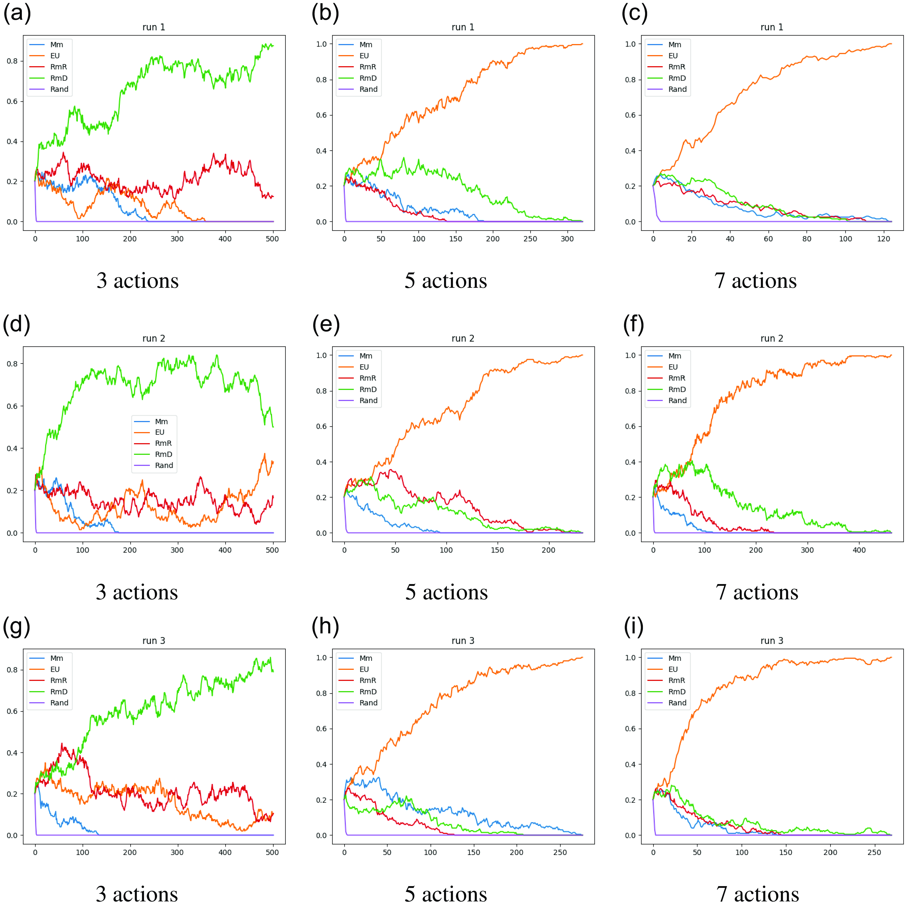
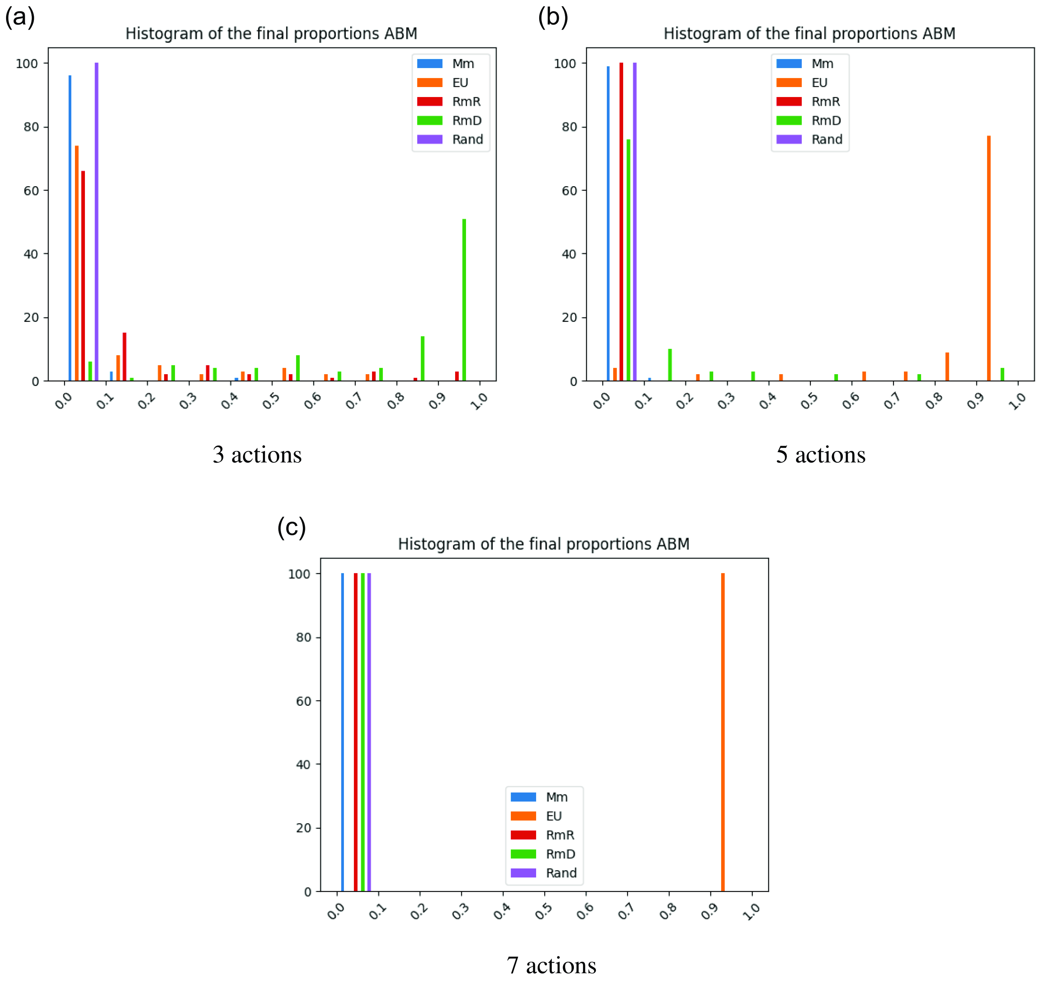


 Open access