


1 Introduction
In the past decades, many injection schemes for electron beams in the accelerating wakefield excited by laser pulses[ Reference Tajima and Dawson 1 – Reference Malka 4 ] have been proposed and tested. Among them, injection by background density variation[ Reference Bulanov, Naumova, Pegoraro and Sakai 5 – Reference Swanson, Tsai, Barber, Lehe, Mao, Steinke, van Tilborg, Nakamura, Geddes, Schroeder, Esarey and Leemans 12 ], collinear colliding pulses injection[ Reference Faure, Rechatin, Norlin, Lifschitz, Glinec and Malka 13 – Reference Hansson, Aurand, Ekerfelt, Persson and Lundh 15 ] and multi-pulse ionization-injection schemes, such as two-color ionization injection[ Reference Yu, Esarey, Schroeder, Vay, Benedetti, Geddes, Chen and Leemans 16 , Reference Schroeder, Benedetti, Esarey, Chen and Leemans 17 ] and resonant multi-pulse ionization injection (ReMPI)[ Reference Tomassini, De Nicola, Labate, Londrillo, Fedele, Terzani and Gizzi 18 – Reference Tomassini, Terzani, Labate, Toci, Chance, Nghiem and Gizzi 20 ], are very promising in terms of transverse beam quality, being able to generate electron beams with normalized emittances as low as tens of nm, as shown by analytical results and numerical simulations. The usage of circularly polarized laser pulses can be beneficial to lower the threshold for self-injection in the bubble regime[ Reference Ma, Seipt, Hussein, Hakimi, Beier, Hansen, Hinojosa, Maksimchuk, Nees, Krushelnick, Thomas and Dollar 21 ]. High-quality ionization injection schemes, however, use linearly polarized pulses for the ionizing pulse to minimize the residual transverse momentum, while they may use either linear or circular polarization for the laser pulse (or the pulse train for the ReMPI scheme), which drives the wakefield[ Reference Yu, Esarey, Schroeder, Vay, Benedetti, Geddes, Chen and Leemans 16 ].
Accuracy of numerical simulations of ionization-injection processes can be extremely challenging when schemes providing good-quality beams are investigated, as they are required to accelerate electron bunches suitable to drive an X-ray free-electron laser[
Reference Wang, Feng, Ke, Yu, Xu, Qi, Chen, Qin, Zhang, Liu, Jiang, Wang, Wang, Yang, Wu, Leng, Liu, Li and Xu
22
] for the EuPRAXIA project[
Reference Assmann, Weikum, Akhter, Alesini, Alexandrova, Anania, Andreev, Andriyash, Artioli, Aschikhin, Audet, Bacci, Barna, Bartocci, Bayramian, Beaton, Beck, Bellaveglia, Beluze, Bernhard, Biagioni, Bielawski, Bisesto, Bonatto, Boulton, Brandi, Brinkmann, Briquez, Brottier, Bründermann, Büscher, Buonomo, Bussmann, Bussolino, Campana, Cantarella, Cassou, Chancé, Chen, Chiadroni, Cianchi, Cioeta, Clarke, Cole, Costa, Couprie, Cowley, Croia, Cros, Crump, D’Arcy, Dattoli, Del Dotto, Delerue, Del Franco, Delinikolas, De Nicola, Dias, Di Giovenale, Diomede, Di Pasquale, Di Pirro, Di Raddo, Dorda, Erlandson, Ertel, Esposito, Falcoz, Falone, Fedele, Pousa, Ferrario, Filippi, Fils, Fiore, Fiorito, Fonseca, Franzini, Galimberti, Gallo, Galvin, Ghaith, Ghigo, Giove, Giribono, Gizzi, Grüner, Habib, Haefner, Heinemann, Helm, Hidding, Holzer, Hooker, Hosokai, Hübner, Ibison, Incremona, Irman, Iungo, Jafarinia, Jakobsson, Jaroszynski, Jaster-Merz, Joshi, Kaluza, Kando, Karger, Karsch, Khazanov, Khikhlukha, Kirchen, Kirwan, Kitégi, Knetsch, Kocon, Koester, Kononenko, Korn, Kostyukov, Kruchinin, Labate, Le Blanc, Lechner, Lee, Leemans, Lehrach, Li, Li, Libov, Lifschitz, Lindstrøm, Litvinenko, Lu, Lundh, Maier, Malka, Manahan, Mangles, Marcelli, Marchetti, Marcouillé, Marocchino, Marteau, de la Ossa, Martins, Mason, Massimo, Mathieu, Maynard, Mazzotta, Mironov, Molodozhentsev, Morante, Mosnier, Mostacci, Müller, Murphy, Najmudin, Nghiem, Nguyen, Niknejadi, Nutter, Osterhoff, Espinos, Paillard, Papadopoulos, Patrizi, Pattathil, Pellegrino, Petralia, Petrillo, Piersanti, Pocsai, Poder, Pompili, Pribyl, Pugacheva, Reagan, Resta-Lopez, Ricci, Romeo, Conti, Rossi, Rossmanith, Rotundo, Roussel, Sabbatini, Santangelo, Sarri, Schaper, Scherkl, Schramm, Schroeder, Scifo, Serafini, Sharma, Sheng, Shpakov, Siders, Silva, Silva, Simon, Simon-Boisson, Sinha, Sistrunk, Specka, Spinka, Stecchi, Stella, Stellato, Streeter, Sutherland, Svystun, Symes, Szwaj, Tauscher, Terzani, Toci, Tomassini, Torres, Ullmann, Vaccarezza, Valléau, Vannini, Vannozzi, Vescovi, Vieira, Villa, Wahlström, Walczak, Walker, Wang, Welsch, Welsch, Weng, Wiggins, Wolfenden, Xia, Yabashi, Zhang, Zhao, Zhu and Zigler
23
] or similar projects based on a high gradient plasma accelerator[
Reference Albert, Couprie, Debus, Downer, Faure, Flacco, Gizzi, Grismayer, Huebl, Joshi, Labat, Leemans, Maier, Mangles, Mason, Mathieu, Muggli, Nishiuchi, Osterhoff, Rajeev, Schramm, Schreiber, Thomas, Vay, Vranic and Zeil
24
]. This is because the longitudinal grid spacing should be small enough to efficiently resolve the extraction process, occurring in a tiny fraction (usually
 $\approx 1/5$
) of the ionization pulse wavelength. The use of reduced envelope models in conjunction with analytical models to correctly mimic the newborn electrons phase-space (e.g., QFluid[
Reference Tomassini, De Nicola, Labate, Londrillo, Fedele, Terzani and Gizzi
18
,
Reference Tomassini and Rossi
25
], INF&RNO[
Reference Benedetti, Schroeder, Esarey, Geddes and Leemans
26
], ALaDyn[
Reference Benedetti, Sgattoni, Turchetti and Londrillo
27
,
Reference Terzani and Londrillo
28
] and Smilei
[
Reference Derouillat, Beck, Pérez, Vinci, Chiaramello, Grassi, Flé, Bouchard, Plotnikov, Aunai, Dargent, Riconda and Grech
29
,
Reference Massimo, Beck, Derouillat, Zemzemi and Specka
30
]) can therefore be advantageous when long and large grid-size simulations are needed. In this respect, highly accurate analytical predictions of the root mean square (rms) transverse momentum or even more accurate models for the phase-space distribution of the extracted electrons are needed. In a seminal paper in 2014, Schroeder et al.[
Reference Schroeder, Vay, Esarey, Benedetti, Chen and Leemans
31
] set for the first time a comprehensive theory of ionization-injection thermal emittance with a single laser pulse. This theory is currently used in the codes cited above and constitutes the state-of-the-art of the analytical results for single pulse ionization-injection schemes, to the best of the authors’ knowledge.
$\approx 1/5$
) of the ionization pulse wavelength. The use of reduced envelope models in conjunction with analytical models to correctly mimic the newborn electrons phase-space (e.g., QFluid[
Reference Tomassini, De Nicola, Labate, Londrillo, Fedele, Terzani and Gizzi
18
,
Reference Tomassini and Rossi
25
], INF&RNO[
Reference Benedetti, Schroeder, Esarey, Geddes and Leemans
26
], ALaDyn[
Reference Benedetti, Sgattoni, Turchetti and Londrillo
27
,
Reference Terzani and Londrillo
28
] and Smilei
[
Reference Derouillat, Beck, Pérez, Vinci, Chiaramello, Grassi, Flé, Bouchard, Plotnikov, Aunai, Dargent, Riconda and Grech
29
,
Reference Massimo, Beck, Derouillat, Zemzemi and Specka
30
]) can therefore be advantageous when long and large grid-size simulations are needed. In this respect, highly accurate analytical predictions of the root mean square (rms) transverse momentum or even more accurate models for the phase-space distribution of the extracted electrons are needed. In a seminal paper in 2014, Schroeder et al.[
Reference Schroeder, Vay, Esarey, Benedetti, Chen and Leemans
31
] set for the first time a comprehensive theory of ionization-injection thermal emittance with a single laser pulse. This theory is currently used in the codes cited above and constitutes the state-of-the-art of the analytical results for single pulse ionization-injection schemes, to the best of the authors’ knowledge.
In the following, we will suppose that the linearly polarized ionization laser pulse of amplitude
 ${a}_0$
, with polarization axis
${a}_0$
, with polarization axis
 $x$
and carrier wavelength
$x$
and carrier wavelength
 ${\lambda}_0$
is propagating along positive
${\lambda}_0$
is propagating along positive
 $z$
. Its amplitude is large enough to provide an electric field above the ionization threshold for the tunnel field-ionization process. Once electrons are extracted from the ions, their dynamics follows the prescription for a generic charged particle in an (almost) plane-wave laser pulse. After averaging the momenta during the whole first laser pulse oscillation, we obtain the initial cycle-average normalized 3D momentum
$z$
. Its amplitude is large enough to provide an electric field above the ionization threshold for the tunnel field-ionization process. Once electrons are extracted from the ions, their dynamics follows the prescription for a generic charged particle in an (almost) plane-wave laser pulse. After averaging the momenta during the whole first laser pulse oscillation, we obtain the initial cycle-average normalized 3D momentum
 $\overrightarrow{u}=\overrightarrow{p}/{m}_{\mathrm{e}}c$
(see Ref. [Reference Massimo, Beck, Derouillat, Zemzemi and Specka30] and references therein):
$\overrightarrow{u}=\overrightarrow{p}/{m}_{\mathrm{e}}c$
(see Ref. [Reference Massimo, Beck, Derouillat, Zemzemi and Specka30] and references therein):
 $$\begin{align}{\overline{u}}_{{x}}=-{a}_{0,\mathrm{e}}\sin {\xi}_{\mathrm{e}},\ {\overline{u}}_{{y}}=0,\ {\overline{u}}_{{z}}=\frac{1}{2}{a}_{0,\mathrm{e}}^2\left({\sin}^2{\xi}_{\mathrm{e}}+\frac{1}{2}\right),\end{align}$$
where
 ${\xi}_{\mathrm{e}}$
is the ionization pulse phase at the extraction time and
${\xi}_{\mathrm{e}}$
is the ionization pulse phase at the extraction time and
 ${a}_{0,\mathrm{e}}$
is the local normalized pulse amplitude at the extraction position. As the electrons slip back in the laser field, their quivering amplitude decreases, while also the longitudinal ponderomotive force gradually reduces the cycle-averaged longitudinal momentum
${a}_{0,\mathrm{e}}$
is the local normalized pulse amplitude at the extraction position. As the electrons slip back in the laser field, their quivering amplitude decreases, while also the longitudinal ponderomotive force gradually reduces the cycle-averaged longitudinal momentum
 ${\overline{u}}_{{z}}$
. Finally, as the pulse completely overpasses the particle, the 3D residual momentum,
${\overline{u}}_{{z}}$
. Finally, as the pulse completely overpasses the particle, the 3D residual momentum,
 $$\begin{align}{u}_{{x}}={\overline{u}}_{{x}},\ {u}_{{y}}={\overline{u}}_{{y}},\ {u}_{{z}}={\overline{u}}_{{z}}-\frac{1}{4}{a}_{0,\mathrm{e}}^2\kern0.1em,\end{align}$$
can be evaluated by neglecting transverse ponderomotive effects and pulse evolution during the slippage. It is worth to note here that, while the (initial) cycle-averaged momentum in Equation (1) is used in, for example, envelope ionization models, the residual momenta of Equation (2) can be employed, in conjunction with the transverse residual position estimate, to evaluate the minimum normalized emittance of the extracted bunch, as in Ref. [Reference Schroeder, Vay, Esarey, Benedetti, Chen and Leemans31].
The theory from Schroeder et al.[
Reference Schroeder, Vay, Esarey, Benedetti, Chen and Leemans
31
] also shows that, in the optimal conditions of unsaturated ionization, the newborn electrons are extracted in tiny slabs centered at the maxima of the electric field strength
 $E=\mid \overrightarrow{E}\left(\overrightarrow{x},t\right)\mid$
. For a given position, and after having defined the phase of
$E=\mid \overrightarrow{E}\left(\overrightarrow{x},t\right)\mid$
. For a given position, and after having defined the phase of
 $E= {E}_0\mid \cos \xi \mid$
such that
$E= {E}_0\mid \cos \xi \mid$
such that
 $\xi =0$
corresponds to a given maximum of
$\xi =0$
corresponds to a given maximum of
 $E$
, the analytical theory shows that the local particle extraction phase
$E$
, the analytical theory shows that the local particle extraction phase
 ${\xi}_{\mathrm{e}}$
shows a Gaussian distribution around
${\xi}_{\mathrm{e}}$
shows a Gaussian distribution around
 ${\xi}_{\mathrm{e}}= n\pi$
, with
${\xi}_{\mathrm{e}}= n\pi$
, with
 $n$
integer and variance
$n$
integer and variance
 ${\sigma}_{\xi}\simeq \Delta$
(note that in Ref. [Reference Schroeder, Vay, Esarey, Benedetti, Chen and Leemans31] the phase extraction variance is named
${\sigma}_{\xi}\simeq \Delta$
(note that in Ref. [Reference Schroeder, Vay, Esarey, Benedetti, Chen and Leemans31] the phase extraction variance is named
 ${\sigma}_{\psi }$
), where
${\sigma}_{\psi }$
), where
 $$\begin{align}\Delta ={\left(\frac{3{E}_0}{2{E}_{\mathrm{a}}}\right)}^{1/2}\cdot {\left(\frac{U_{\mathrm{H}}}{U_{\mathrm{I}}}\right)}^{3/4}.\end{align}$$
Here,
 ${E}_0$
is the ionization pulse strength,
${E}_0$
is the ionization pulse strength,
 ${E}_{\mathrm{a}}\simeq 0.51\kern0.24em \mathrm{TV}/\mathrm{m}$
is the atomic field strength and
${E}_{\mathrm{a}}\simeq 0.51\kern0.24em \mathrm{TV}/\mathrm{m}$
is the atomic field strength and
 ${U}_{\mathrm{H},\mathrm{I}}$
are the ionization potentials of hydrogen and of the atomic selected level to be ionized, respectively. Consequently, the rms residual particle momentum
${U}_{\mathrm{H},\mathrm{I}}$
are the ionization potentials of hydrogen and of the atomic selected level to be ionized, respectively. Consequently, the rms residual particle momentum
 ${\sigma}_{{{u}}_{{x}}}=\sqrt{\left\langle {\left({u}_{{x}}\right)}^2\right\rangle }$
along the ionization pulse polarization is approximately
${\sigma}_{{{u}}_{{x}}}=\sqrt{\left\langle {\left({u}_{{x}}\right)}^2\right\rangle }$
along the ionization pulse polarization is approximately
 ${a}_0\Delta$
. High-quality electron bunches are obtained by minimizing the transverse rms momentum, and this is accomplished by a minimization of
${a}_0\Delta$
. High-quality electron bunches are obtained by minimizing the transverse rms momentum, and this is accomplished by a minimization of
 ${\sigma}_{\xi }$
, which should assume the lowest possible value compatible with the possibility of extracting the electrons from the selected atomic level of the dopant atoms. As an example,
${\sigma}_{\xi }$
, which should assume the lowest possible value compatible with the possibility of extracting the electrons from the selected atomic level of the dopant atoms. As an example,
 ${\mathrm{N}}^{5^{+}\to {6}^{+}}$
,
${\mathrm{N}}^{5^{+}\to {6}^{+}}$
,
 ${\mathrm{Ar}}^{8^{+}\to {9}^{+}}$
and
${\mathrm{Ar}}^{8^{+}\to {9}^{+}}$
and
 $\mathrm{Kr}^{8^{+}\to {9}^{+}}$
transitions are usually employed in ReMPI or two-color schemes. The optimal values of
$\mathrm{Kr}^{8^{+}\to {9}^{+}}$
transitions are usually employed in ReMPI or two-color schemes. The optimal values of
 $\Delta \simeq {\sigma}_{\xi }$
for those processes are approximately 0.29, 0.24 and 0.22, respectively (see below).
$\Delta \simeq {\sigma}_{\xi }$
for those processes are approximately 0.29, 0.24 and 0.22, respectively (see below).
The possibility of using very accurate predictors of the rms normalized emittance along the polarization axis for either particles extracted in a single cycle or by the whole laser pulse is of paramount importance for high-quality beam production studies. Moreover, as standard requests refer to both high charge and high quality for the beam, working points in a saturated or partially saturated regime are often selected. Motivated by the needs reported above, we recast the theory in Ref. [Reference Schroeder, Vay, Esarey, Benedetti, Chen and Leemans31] for the local and global bunch parameters, so as to include all the relevant terms of order
 ${\Delta}^2$
, and to include additional
${\Delta}^2$
, and to include additional
 ${\Delta}^4$
terms. In this work, we addressed the need for high-accuracy rms predictors in the unsaturated regime, with errors between analytical results and numerical simulations below
${\Delta}^4$
terms. In this work, we addressed the need for high-accuracy rms predictors in the unsaturated regime, with errors between analytical results and numerical simulations below
 $1\%$
(see Sections 3.1 and 4.1). As high-charge beams are needed, however, higher pulse amplitudes are used so as to extract more charge, therefore exploring partially or even fully saturated regimes. There, a gradual increase of the global normalized emittance is found by simulations, as already pointed out in Ref. [Reference Schroeder, Vay, Esarey, Benedetti, Chen and Leemans31]. Our analytical theory that includes global saturation effects confirms the emittance increase and very accurately fits the simulation results (see Section 4.2). Moving with increasingly higher amplitudes, we explore the saturation limit within a single laser cycle. The phase-space of the electrons extracted in a single-cycle saturated regime (see Section 3.2) reveals fine structures that may help the understanding of either experimental[
Reference Guénot, Gustas, Vernier, Beaurepaire, Böhle, Bocoum, Lozano, Jullien, Lopez-Martens, Lifschitz and Faure
32
,
Reference Faure, Gustas, Guénot, Vernier, Böhle, Ouillé, Haessler, Lopez-Martens and Lifschitz
33
] or particle-in-cell (PIC) simulation[
Reference Lifschitz and Malka
34
] results when high-intensity, very short pulses are used. Our model for the phase-space is revealed to be extremely accurate in this regime too (see Section 3.2), and predicts a reduction of the transverse momentum once the fully saturated regime is reached. Very large pulse amplitudes, however, may lead to switching on multiple ionization stages. In this work we also propose an accurate model for this double-ionization process (see Section 3.3). Although the theory proposed in this work only considers the effects of the laser pulse, it is interesting to compare the results concerning the whole bunch emittance with those obtained by PIC simulations, including the plasma wakefield contribution (Section 5), with a focus on sub-micrometer long bunches obtainable with the ReMPI scheme.
$1\%$
(see Sections 3.1 and 4.1). As high-charge beams are needed, however, higher pulse amplitudes are used so as to extract more charge, therefore exploring partially or even fully saturated regimes. There, a gradual increase of the global normalized emittance is found by simulations, as already pointed out in Ref. [Reference Schroeder, Vay, Esarey, Benedetti, Chen and Leemans31]. Our analytical theory that includes global saturation effects confirms the emittance increase and very accurately fits the simulation results (see Section 4.2). Moving with increasingly higher amplitudes, we explore the saturation limit within a single laser cycle. The phase-space of the electrons extracted in a single-cycle saturated regime (see Section 3.2) reveals fine structures that may help the understanding of either experimental[
Reference Guénot, Gustas, Vernier, Beaurepaire, Böhle, Bocoum, Lozano, Jullien, Lopez-Martens, Lifschitz and Faure
32
,
Reference Faure, Gustas, Guénot, Vernier, Böhle, Ouillé, Haessler, Lopez-Martens and Lifschitz
33
] or particle-in-cell (PIC) simulation[
Reference Lifschitz and Malka
34
] results when high-intensity, very short pulses are used. Our model for the phase-space is revealed to be extremely accurate in this regime too (see Section 3.2), and predicts a reduction of the transverse momentum once the fully saturated regime is reached. Very large pulse amplitudes, however, may lead to switching on multiple ionization stages. In this work we also propose an accurate model for this double-ionization process (see Section 3.3). Although the theory proposed in this work only considers the effects of the laser pulse, it is interesting to compare the results concerning the whole bunch emittance with those obtained by PIC simulations, including the plasma wakefield contribution (Section 5), with a focus on sub-micrometer long bunches obtainable with the ReMPI scheme.
2 Setting up the pulse amplitude for tunnel ionization
In the following, the tunnel ionization process occurring in a (single) laser field is considered. The instantaneous ionization rate can be described by the Ammosov–Delone–Krainov (ADK) formula[
Reference Perelomov, Popov and Terent’ev
35
–
Reference Nuter, Gremillet, Lefebvre, Lévy, Ceccotti and Martin
38
], expressed in terms of the electric field normalized to the critical ADK field
 ${\rho}_0\equiv \frac{3E}{2{E}_{\mathrm{a}}}{\left(\frac{U_{\mathrm{H}}}{U_{\mathrm{I}}}\right)}^{3/2}={a}_0/{a}_{\mathrm{c}}$
(here
${\rho}_0\equiv \frac{3E}{2{E}_{\mathrm{a}}}{\left(\frac{U_{\mathrm{H}}}{U_{\mathrm{I}}}\right)}^{3/2}={a}_0/{a}_{\mathrm{c}}$
(here
 ${a}_{\mathrm{c}}\simeq 0.107{\lambda}_0{\left(\frac{U_{\mathrm{I}}}{U_{\mathrm{H}}}\right)}^{3/2}$
), introduced in Ref. [Reference Tomassini, De Nicola, Labate, Londrillo, Fedele, Terzani and Gizzi18]:
${a}_{\mathrm{c}}\simeq 0.107{\lambda}_0{\left(\frac{U_{\mathrm{I}}}{U_{\mathrm{H}}}\right)}^{3/2}$
), introduced in Ref. [Reference Tomassini, De Nicola, Labate, Londrillo, Fedele, Terzani and Gizzi18]:
 $$\begin{align}\displaystyle\frac{\textrm{d}n_{\mathrm{e}}}{\textrm{d}t} &= W\cdot \left({n}_{0,\mathrm{i}}-{n}_{\mathrm{e}}\right),\nonumber\\ {}W&=C{\left({\rho}_0|\cos \xi |\right)}^{\mu}\exp \left(-\displaystyle\frac{1}{\rho_0\mid \cos \xi \mid}\right),\end{align}$$
where
 ${n}_{\mathrm{e}}$
is the number of extracted particles and
${n}_{\mathrm{e}}$
is the number of extracted particles and
 ${n}_{0,\mathrm{i}}$
is the initial number of available ions;
${n}_{0,\mathrm{i}}$
is the initial number of available ions;
 $C$
depends on the atom species and ionization level (there are some different versions for
$C$
depends on the atom species and ionization level (there are some different versions for
 $C$
, e.g., Equation (6) in Ref. [Reference Tomassini, De Nicola, Labate, Londrillo, Fedele, Terzani and Gizzi18]). The exponent
$C$
, e.g., Equation (6) in Ref. [Reference Tomassini, De Nicola, Labate, Londrillo, Fedele, Terzani and Gizzi18]). The exponent
 $\mu$
in Equation (4) is defined as follows:
$\mu$
in Equation (4) is defined as follows:
 $$\begin{align}\mu =-2{n}^{\ast }+\mid m\mid +1,\end{align}$$
with
 ${n}^{\ast}=Z\sqrt{U_{\mathrm{H}}/{U}_{\mathrm{I}}}$
and
${n}^{\ast}=Z\sqrt{U_{\mathrm{H}}/{U}_{\mathrm{I}}}$
and
 $m$
being the effective principal quantum number of the ion with final charge
$m$
being the effective principal quantum number of the ion with final charge
 $Ze$
and the projection of the angular momentum, respectively. The peak normalized amplitude
$Ze$
and the projection of the angular momentum, respectively. The peak normalized amplitude
 ${\rho}_0={a}_0/{a}_{\mathrm{c}}$
is related to the
${\rho}_0={a}_0/{a}_{\mathrm{c}}$
is related to the
 $\Delta$
term in Ref. [Reference Schroeder, Vay, Esarey, Benedetti, Chen and Leemans31] as
$\Delta$
term in Ref. [Reference Schroeder, Vay, Esarey, Benedetti, Chen and Leemans31] as
 ${\rho}_0={\Delta}^2$
. The evaluation of the number of extracted electrons and spatial averages of
${\rho}_0={\Delta}^2$
. The evaluation of the number of extracted electrons and spatial averages of
 ${\sigma}_{{{u}}_{{x}}}$
will be strongly simplified by expressing the average ionization rate over a single ionization pulse cycle
${\sigma}_{{{u}}_{{x}}}$
will be strongly simplified by expressing the average ionization rate over a single ionization pulse cycle
 $\left\langle W\left({\rho}_0\right)\right\rangle$
as follows:
$\left\langle W\left({\rho}_0\right)\right\rangle$
as follows:
 $$\begin{align}\left\langle W\right\rangle &\equiv \displaystyle\frac{1}{\pi }{\displaystyle\int}_{-\pi /2}^{\pi /2}W\left({\rho}_0,\xi \right) \textrm{d}\xi \nonumber\\ & \simeq C\sqrt{\displaystyle\frac{2}{\pi }}\left(1-\displaystyle\frac{\mu +5/4}{2}{\rho}_0\right){\rho}_0^{\mu +1/2}{e}^{-1/{\rho}_0}.\end{align}$$
The choice of the optimal value for the normalized field amplitude
 ${\rho}_0={\Delta}^2$
depends on several parameters, including the number of extracted electrons, the final needed beam quality, the ion density, pulse peak electric field and size. If a large number of electrons have to be extracted, an optimal working point could be set so that the laser pulse is close to its saturation limit, that is, a large fraction of the ions in the vicinity of the pulse axis are ionized after the pulse passage. The solution of Equation (4) for an ionization depth
${\rho}_0={\Delta}^2$
depends on several parameters, including the number of extracted electrons, the final needed beam quality, the ion density, pulse peak electric field and size. If a large number of electrons have to be extracted, an optimal working point could be set so that the laser pulse is close to its saturation limit, that is, a large fraction of the ions in the vicinity of the pulse axis are ionized after the pulse passage. The solution of Equation (4) for an ionization depth
 $L$
is
$L$
is
 ${n}_{\mathrm{e}}(L)={n}_{0,\mathrm{i}}[1-{e}^{-\overline{\Gamma}\left({L}\right)}]$
with the following:
${n}_{\mathrm{e}}(L)={n}_{0,\mathrm{i}}[1-{e}^{-\overline{\Gamma}\left({L}\right)}]$
with the following:
 $$\begin{align}\overline{\Gamma}(L)={\int}_0^{{L}} \textrm{d}z\left\langle W\right\rangle /c.\end{align}$$
Setting
 $\overline{\Gamma}=1$
, we get an ionization percentage of approximately equal to
$\overline{\Gamma}=1$
, we get an ionization percentage of approximately equal to
 $60\%$
, and therefore
$60\%$
, and therefore
 $\overline{\Gamma}(L)\approx 1$
can be used to define the threshold of saturation effects. It is worth defining the local average ionization rate
$\overline{\Gamma}(L)\approx 1$
can be used to define the threshold of saturation effects. It is worth defining the local average ionization rate
 $\left\langle W\right\rangle /c$
as
$\left\langle W\right\rangle /c$
as
 $\left\langle W\right\rangle /c\equiv {\overline{k}}_{\mathrm{ADK}}{\rho}_0^{\mu +1/2}{e}^{-1/{\rho}_0}$
, where:
$\left\langle W\right\rangle /c\equiv {\overline{k}}_{\mathrm{ADK}}{\rho}_0^{\mu +1/2}{e}^{-1/{\rho}_0}$
, where:
 $$\begin{align}{\overline{k}}_{\mathrm{ADK}}=\sqrt{\frac{2}{\pi }}C\left(|m|\right)/c.\end{align}$$
We are now able to find the normalized field achieving a saturation percentage approximately equal to
 $60\%$
in a longitudinal length
$60\%$
in a longitudinal length
 $L$
. For the selected processes of
$L$
. For the selected processes of
 ${\mathrm{Kr}}^{8^{+}\to {9}^{+}}\left(m=0\right)$
,
${\mathrm{Kr}}^{8^{+}\to {9}^{+}}\left(m=0\right)$
,
 ${\mathrm{Ar}}^{8^{+}\to {9}^{+}}\left(m=0\right)$
and
${\mathrm{Ar}}^{8^{+}\to {9}^{+}}\left(m=0\right)$
and
 ${\mathrm{N}}^{5^{+}\to {6}^{+}}\left(m=0\right)$
, the
${\mathrm{N}}^{5^{+}\to {6}^{+}}\left(m=0\right)$
, the
 ${\overline{k}}_{\mathrm{ADK}}$
parameters evaluated with Equation (2) in Ref. [Reference Schroeder, Vay, Esarey, Benedetti, Chen and Leemans31] are
${\overline{k}}_{\mathrm{ADK}}$
parameters evaluated with Equation (2) in Ref. [Reference Schroeder, Vay, Esarey, Benedetti, Chen and Leemans31] are
 $1.8\times {10}^5$
,
$1.8\times {10}^5$
,
 $1.4\times {10}^5$
,
$1.4\times {10}^5$
,
 $0.24\times {10}^5\;{\unicode{x3bc} \mathrm{m}}^{-1}$
, respectively. For each ionization process and saturation length
$0.24\times {10}^5\;{\unicode{x3bc} \mathrm{m}}^{-1}$
, respectively. For each ionization process and saturation length
 $L$
, the normalized field
$L$
, the normalized field
 ${\rho}_0={a}_0/{a}_{\mathrm{c}}$
reaching saturation can be obtained by numerical solution of the following equation:
${\rho}_0={a}_0/{a}_{\mathrm{c}}$
reaching saturation can be obtained by numerical solution of the following equation:
 $$\begin{align}\left({\overline{k}}_{\mathrm{ADK}}L\right){\rho}_0^{\mu +1/2}{e}^{-1/{\rho}_0}=1.\end{align}$$
Graphical solutions of Equation (9) for either tens of fs long pulses or near single-cycle pulses can be found in the Appendix.
3 Accurate residual momentum theory for single-cycle lasting ionization
In this section we recast the theory for
 ${\sigma}_{{{u}}_{{x}}}$
and improve its accuracy by (i) including an
${\sigma}_{{{u}}_{{x}}}$
and improve its accuracy by (i) including an
 $\mathcal{O}\left({\Delta}^2\right)$
term not taken into account in Ref. [Reference Schroeder, Vay, Esarey, Benedetti, Chen and Leemans31], (ii) extending the theory up to
$\mathcal{O}\left({\Delta}^2\right)$
term not taken into account in Ref. [Reference Schroeder, Vay, Esarey, Benedetti, Chen and Leemans31], (ii) extending the theory up to
 $\mathcal{O}\left({\Delta}^4\right)$
terms and, finally, (iii) including (exponential) correction terms due to the onset of saturation effects. We will start with local properties of the emitted electrons by neglecting the saturation effects. Afterwards, we include the onset of saturation contribution for
$\mathcal{O}\left({\Delta}^4\right)$
terms and, finally, (iii) including (exponential) correction terms due to the onset of saturation effects. We will start with local properties of the emitted electrons by neglecting the saturation effects. Afterwards, we include the onset of saturation contribution for
 ${\sigma}_{{{u}}_{{x}}}$
. The new analytical results can therefore be included in envelope codes aiming at an accurate statistical reconstruction of the ionization process even at ionization pulse intensities close to the single-cycle saturation threshold (see below).
${\sigma}_{{{u}}_{{x}}}$
. The new analytical results can therefore be included in envelope codes aiming at an accurate statistical reconstruction of the ionization process even at ionization pulse intensities close to the single-cycle saturation threshold (see below).
3.1 Local properties of the emitted electrons without saturation effects
We start considering the rms values of the extraction phase
 $\xi$
(
$\xi$
(
 ${\sigma}_{\psi }$
in Ref. [Reference Schroeder, Vay, Esarey, Benedetti, Chen and Leemans31]) and of
${\sigma}_{\psi }$
in Ref. [Reference Schroeder, Vay, Esarey, Benedetti, Chen and Leemans31]) and of
 $\sin \xi$
, with the aim of obtaining an approximate result including
$\sin \xi$
, with the aim of obtaining an approximate result including
 $\mathcal{O}\left({\Delta}^4\right)$
(i.e.,
$\mathcal{O}\left({\Delta}^4\right)$
(i.e.,
 $\mathcal{O}\left({\rho}_0^2\right)$
) corrections for the latter, but neglecting the ionization saturation effects. Following Ref. [Reference Schroeder, Vay, Esarey, Benedetti, Chen and Leemans31], we consider a single half-cycle of the ionization pulse
$\mathcal{O}\left({\rho}_0^2\right)$
) corrections for the latter, but neglecting the ionization saturation effects. Following Ref. [Reference Schroeder, Vay, Esarey, Benedetti, Chen and Leemans31], we consider a single half-cycle of the ionization pulse
 $E\left(\xi \right)={E}_0\cos \xi$
, extracting electrons with phases
$E\left(\xi \right)={E}_0\cos \xi$
, extracting electrons with phases
 $\xi ={k}_0\left(z- ct\right)$
around the field maximum at
$\xi ={k}_0\left(z- ct\right)$
around the field maximum at
 $\xi =0$
. Expressing the ionization rate
$\xi =0$
. Expressing the ionization rate
 $W\left(\xi \right)$
in terms of the extraction phase, we get the following:
$W\left(\xi \right)$
in terms of the extraction phase, we get the following:
 $$\begin{align}W\left(\xi \right)&={W}_0\cdot {\left(\cos \xi \right)}^{\mu}\exp \left[\displaystyle\frac{1}{\rho_0}\left(\displaystyle\frac{1}{\cos \xi }-1\right)\right]\nonumber\\ &\simeq {W}_0\exp \left(-\displaystyle\frac{\xi^2}{2{\rho}_0}\right)\left(1-\displaystyle\frac{\mu }{2}{\xi}^2-\displaystyle\frac{5}{24{\rho}_0}{\xi}^4\right)\nonumber\\ &\simeq {W}_0\exp \left[-\displaystyle\frac{\xi^2}{2{\sigma}_{\psi}^2}\left(1+\displaystyle\frac{5}{12}{\xi}^2\right)\right],\end{align}$$
where
 ${W}_0\equiv W\left(\xi =0\right)={k}_{\mathrm{ADK}}/{k}_0{\rho}_0^{\mu }{e}^{-1/{\rho}_0}$
is the maximum rate for the given pulse strength and
${W}_0\equiv W\left(\xi =0\right)={k}_{\mathrm{ADK}}/{k}_0{\rho}_0^{\mu }{e}^{-1/{\rho}_0}$
is the maximum rate for the given pulse strength and
 ${\sigma}_{\psi}^{-2}={\rho}_0^{-1}\left(1+{\mu \rho}_0\right)$
is the same expression as Equation (6) in Ref. [Reference Schroeder, Vay, Esarey, Benedetti, Chen and Leemans31]. The expansion of the exponential factor in Equation (10) in powers of
${\sigma}_{\psi}^{-2}={\rho}_0^{-1}\left(1+{\mu \rho}_0\right)$
is the same expression as Equation (6) in Ref. [Reference Schroeder, Vay, Esarey, Benedetti, Chen and Leemans31]. The expansion of the exponential factor in Equation (10) in powers of
 $\xi$
is justified by the fact that
$\xi$
is justified by the fact that
 ${\rho}_0={\Delta}^2\ll 1$
in our regimes. Here, terms containing
${\rho}_0={\Delta}^2\ll 1$
in our regimes. Here, terms containing
 ${\xi}^4/{\rho}_0$
are retained as they are
${\xi}^4/{\rho}_0$
are retained as they are
 $\mathcal{O}\left({\Delta}^2\right)$
and this is related to the difference of our results from the equivalent terms in Ref. [Reference Schroeder, Vay, Esarey, Benedetti, Chen and Leemans31] (see below). From now on, we will use
$\mathcal{O}\left({\Delta}^2\right)$
and this is related to the difference of our results from the equivalent terms in Ref. [Reference Schroeder, Vay, Esarey, Benedetti, Chen and Leemans31] (see below). From now on, we will use
 $W\left(\xi \right)$
in the form
$W\left(\xi \right)$
in the form
 ${W}_0{e}^{-\frac{\xi^2}{2{\rho}_0}}\left(1-\frac{\mu }{2}{\xi}^2-\frac{5}{24{\rho}_0}{\xi}^4\right)$
, which results to be corrected up to
${W}_0{e}^{-\frac{\xi^2}{2{\rho}_0}}\left(1-\frac{\mu }{2}{\xi}^2-\frac{5}{24{\rho}_0}{\xi}^4\right)$
, which results to be corrected up to
 $\mathcal{O}\left({\rho}_0^2\right)$
.
$\mathcal{O}\left({\rho}_0^2\right)$
.
It is now straightforward to evaluate the expectation values of
 ${\xi}^2$
, obtaining (up to
${\xi}^2$
, obtaining (up to
 $\mathcal{O}\left({\Delta}^2\right)$
) the following:
$\mathcal{O}\left({\Delta}^2\right)$
) the following:
 $$\begin{align}{\sigma}_{\xi, 0}^2\equiv \left\langle {\xi}^2\right\rangle ={\rho}_0\left[1-\left(\mu +5/2\right){\rho}_0\right].\end{align}$$
Our expression of
 $\left\langle {\xi}^2\right\rangle$
differs from the result in Ref. [Reference Schroeder, Vay, Esarey, Benedetti, Chen and Leemans31] by the presence of the additional
$\left\langle {\xi}^2\right\rangle$
differs from the result in Ref. [Reference Schroeder, Vay, Esarey, Benedetti, Chen and Leemans31] by the presence of the additional
 $\left(-5/2\right){\rho}_0$
term.
$\left(-5/2\right){\rho}_0$
term.
The rms residual momentum
 ${u}_x=-{a}_0\sin \xi$
is, however, directly related to the sinus of the extraction phase
${u}_x=-{a}_0\sin \xi$
is, however, directly related to the sinus of the extraction phase
 $\xi$
. Including all the correction terms up to
$\xi$
. Including all the correction terms up to
 ${\rho}_0^2$
but neglecting ponderomotive force and saturation contributions, we get
${\rho}_0^2$
but neglecting ponderomotive force and saturation contributions, we get
 ${\sigma}_{u,0}^2\equiv \left\langle {u}_x^2\right\rangle ={a}_0^2{\sigma}_{s,0}^2$
, where
${\sigma}_{u,0}^2\equiv \left\langle {u}_x^2\right\rangle ={a}_0^2{\sigma}_{s,0}^2$
, where
 $$\begin{align}{\sigma}_{s,0}^2\equiv \left\langle {\sin}^2\xi \right\rangle ={\rho}_0\left(1+{s}_\textrm{I}\cdot {\rho}_0+{s}_{\textrm{II}}\cdot {\rho}_0^2\right),\end{align}$$
where
 ${s}_\textrm{I}=-\left(\mu +5/2+1\right)$
and
${s}_\textrm{I}=-\left(\mu +5/2+1\right)$
and
 ${s}_{\textrm{II}}=\frac{1}{8}\left(8{\mu}^2+68\mu +131\right)$
. Once again, our expression up to the correction
${s}_{\textrm{II}}=\frac{1}{8}\left(8{\mu}^2+68\mu +131\right)$
. Once again, our expression up to the correction
 $\mathcal{O}\left({\rho}_0\right)$
differs by the equivalent in Ref. [Reference Schroeder, Vay, Esarey, Benedetti, Chen and Leemans31] by the presence of the
$\mathcal{O}\left({\rho}_0\right)$
differs by the equivalent in Ref. [Reference Schroeder, Vay, Esarey, Benedetti, Chen and Leemans31] by the presence of the
 $\left(-5/2\right){\rho}_0$
term. Figure 1 shows the dependence of
$\left(-5/2\right){\rho}_0$
term. Figure 1 shows the dependence of
 ${\sigma}_{\xi, 0}$
and
${\sigma}_{\xi, 0}$
and
 ${\sigma}_{s,0}$
on the pulse amplitude
${\sigma}_{s,0}$
on the pulse amplitude
 ${a}_0$
for the local extraction of particles by the process
${a}_0$
for the local extraction of particles by the process
 ${\mathrm{Ar}}^{8^{+}\to {9}^{+}}$
and a pulse with wavelength
${\mathrm{Ar}}^{8^{+}\to {9}^{+}}$
and a pulse with wavelength
 ${\lambda}_0=0.4\ \unicode{x3bc} \mathrm{m}$
. For both central moments, the theory is able to reproduce the Monte Carlo simulations results with high accuracy.
${\lambda}_0=0.4\ \unicode{x3bc} \mathrm{m}$
. For both central moments, the theory is able to reproduce the Monte Carlo simulations results with high accuracy.
Root mean square values of the local extraction phases
 ${\xi}_\textrm{e}$
and their sinus as a function of the laser amplitude
${\xi}_\textrm{e}$
and their sinus as a function of the laser amplitude
 ${a}_0$
(
${a}_0$
(
 ${\lambda}_0=0.4\;\unicode{x3bc} \mathrm{m}$
) for the process
${\lambda}_0=0.4\;\unicode{x3bc} \mathrm{m}$
) for the process
 $\mathrm{Ar}^{8^{+}\to {9}^{+}}$
. The blue line shows the analytical results for
$\mathrm{Ar}^{8^{+}\to {9}^{+}}$
. The blue line shows the analytical results for
 ${\sigma}_{\xi, 0}$
by Equation (11), while the orange line represents the analytical results for
${\sigma}_{\xi, 0}$
by Equation (11), while the orange line represents the analytical results for
 ${\sigma}_{{s},0}$
by Equation (12). Results from Monte Carlo simulations (green diamonds and red circles, respectively) well agree with the theory. The black dash-dotted line refers to the bare (lowest order) estimation of
${\sigma}_{{s},0}$
by Equation (12). Results from Monte Carlo simulations (green diamonds and red circles, respectively) well agree with the theory. The black dash-dotted line refers to the bare (lowest order) estimation of
 ${\sigma}_{\xi, 0}\simeq {\sigma}_{s,0}\simeq {\Delta}_0=\sqrt{\rho_0}$
.
${\sigma}_{\xi, 0}\simeq {\sigma}_{s,0}\simeq {\Delta}_0=\sqrt{\rho_0}$
.

3.2 Local, single-channel, ionization process including saturation effects
Local saturation effects may be important when they occur within a single pulse cycle (see Figure 2). In this case, due to the monotonic reduction of the available ions as the pulse proceeds crossing each field peak, an asymmetry of the extraction average phase occurs, thus inducing a deviation of the rms value for
 ${u}_x$
(see below) from the unsaturated case and the occurrence of a nonzero average momentum along the polarization axis. In this section we explore the local ionization process occurring in a single channel (e.g.,
${u}_x$
(see below) from the unsaturated case and the occurrence of a nonzero average momentum along the polarization axis. In this section we explore the local ionization process occurring in a single channel (e.g.,
 $\mathrm{Ar}^{8^{+}\to {9}^{+}}$
), while multiple ionization processes activated by the very large electric field will be discussed in the next section.
$\mathrm{Ar}^{8^{+}\to {9}^{+}}$
), while multiple ionization processes activated by the very large electric field will be discussed in the next section.
Going more into detail with the rate equation (4), we start expressing the integral
 $\int \left({\textrm{d}n}_\textrm{e}/ \textrm{d}t\right) \textrm{d}t$
as follows:
$\int \left({\textrm{d}n}_\textrm{e}/ \textrm{d}t\right) \textrm{d}t$
as follows:
 $$\begin{align}\Gamma \left(\xi \right)&\equiv \displaystyle\frac{1}{k_{0,x}}{\displaystyle\int}_{-\pi /2}^{\xi } \textrm{d}x W(x)\nonumber\\ &=\displaystyle\frac{k_{\textrm{ADK}}}{k_0}{\rho}_0^{\mu }{\displaystyle\int}_{-\pi /2}^{\xi } \textrm{d}x{\left(\cos x\right)}^{\mu }{e}^{-\displaystyle\frac{1}{\rho_0\cos x}}\nonumber\\ &\simeq {\nu}_{\mathrm{s}}\left({\rho}_0\right)\mathcal{G}\left(\displaystyle\frac{\xi }{\sqrt{2{\rho}_0}}\right),\end{align}$$
where
 $$\begin{align}\mathcal{G}(x)\equiv \frac{1}{2}\left[1+\operatorname{erf}(x)\right]+\frac{\rho_0}{24\sqrt{\pi }}x\left(15+12\mu +10{x}^2\right){e}^{-{x}^2}\end{align}$$
is the saturation shape function,
 $\operatorname{erf}(x)$
is the error function and
$\operatorname{erf}(x)$
is the error function and
 ${k}_{\mathrm{ADK}}=C\left(|m|\right)/c$
and
${k}_{\mathrm{ADK}}=C\left(|m|\right)/c$
and
 ${\rho}_0\ll 1$
have been used in the last manipulation. In Equation (13) we have also introduced the saturation parameter
${\rho}_0\ll 1$
have been used in the last manipulation. In Equation (13) we have also introduced the saturation parameter
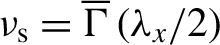 ${\nu}_{\mathrm{s}}=\overline{\Gamma}\left({\lambda}_x/2\right)$
(see Equations (6) and (7)):
${\nu}_{\mathrm{s}}=\overline{\Gamma}\left({\lambda}_x/2\right)$
(see Equations (6) and (7)):
Cumulative ionization fraction
 $\Gamma \left(\xi \right)$
(see Equation (13)) evaluated numerically from the exact weight (red curve), from theory (blue curve) and by theory without the
$\Gamma \left(\xi \right)$
(see Equation (13)) evaluated numerically from the exact weight (red curve), from theory (blue curve) and by theory without the
 ${\xi}^4/{\rho}_0$
term (orange full-dashed line). The right-hand axis shows the errors associated either with the theory (black curve) or with the lower order theory without the non-Gaussian
${\xi}^4/{\rho}_0$
term (orange full-dashed line). The right-hand axis shows the errors associated either with the theory (black curve) or with the lower order theory without the non-Gaussian
 ${e}^{-5{\xi}^4/\left(24{\rho}_0\right)}$
correction.
${e}^{-5{\xi}^4/\left(24{\rho}_0\right)}$
correction.

 $$\begin{align}{\nu}_{\mathrm{s}}\equiv \sqrt{2\pi}\frac{{k}_{\mathrm{ADK}}}{k_0}\left(1-\frac{\mu +5/4}{2}{\rho}_0\right){\rho}_0^{\mu +1/2}{e}^{-\frac{1}{\rho_0}}.\end{align}$$
The saturation shape function
 $\mathcal{G}\left(\frac{\xi }{\sqrt{2{\rho}_0}}\right)$
accurately describes the particle extraction as the phase proceeds from
$\mathcal{G}\left(\frac{\xi }{\sqrt{2{\rho}_0}}\right)$
accurately describes the particle extraction as the phase proceeds from
 $-\pi /2$
to
$-\pi /2$
to
 $\xi$
within a single half-pulse cycle and satisfies
$\xi$
within a single half-pulse cycle and satisfies
 $\mathcal{G}\left(\frac{-\pi /2}{\sqrt{2{\rho}_0}}\right)=0$
,
$\mathcal{G}\left(\frac{-\pi /2}{\sqrt{2{\rho}_0}}\right)=0$
,
 $\mathcal{G}\left(\frac{\pi /2}{\sqrt{2{\rho}_0}}\right)=1$
, provided that
$\mathcal{G}\left(\frac{\pi /2}{\sqrt{2{\rho}_0}}\right)=1$
, provided that
 ${\rho}_0\ll 1$
. As is apparent in Figure 3, the full expression for
${\rho}_0\ll 1$
. As is apparent in Figure 3, the full expression for
 $\mathcal{G}\left(\frac{\xi }{\sqrt{2{\rho}_0}}\right)$
predicts the (numerically evaluated) exact values for
$\mathcal{G}\left(\frac{\xi }{\sqrt{2{\rho}_0}}\right)$
predicts the (numerically evaluated) exact values for
 $\Gamma \left(\xi \right)$
with errors
$\Gamma \left(\xi \right)$
with errors
 $\mathcal{O}\left({\rho}_0^2\right)$
, while the more simple expression
$\mathcal{O}\left({\rho}_0^2\right)$
, while the more simple expression
 $$\begin{align}{\mathcal{G}}_0(x)\equiv \frac{1}{2}\left[1+\operatorname{erf}(x)\right]\end{align}$$
is also an accurate predictor, but with expected errors
 $\mathcal{O}\left({\rho}_0\right)$
.
$\mathcal{O}\left({\rho}_0\right)$
.
Statistical moments
 $\Xi \left(n,{\rho}_0\right)$
for
$\Xi \left(n,{\rho}_0\right)$
for
 $n=1{-}4$
and full saturation correction
$n=1{-}4$
and full saturation correction
 $S$
numerically evaluated as in Equations (20) and (25) as a function of the saturation parameter
$S$
numerically evaluated as in Equations (20) and (25) as a function of the saturation parameter
 ${\nu}_{\mathrm{s}}$
for the transition
${\nu}_{\mathrm{s}}$
for the transition
 $\mathrm{Ar}^{8^{+}\to {9}^{+}}$
and
$\mathrm{Ar}^{8^{+}\to {9}^{+}}$
and
 ${\lambda}_0=0.4\ \unicode{x3bc} \mathrm{m}$
.
${\lambda}_0=0.4\ \unicode{x3bc} \mathrm{m}$
.

Once the cumulative ionization function
 $\Gamma \left(\xi \right)$
has been obtained, the newborn electron distribution function equation, including saturation effects, can be evaluated as
$\Gamma \left(\xi \right)$
has been obtained, the newborn electron distribution function equation, including saturation effects, can be evaluated as
 $$\begin{align}\frac{1}{n_{0,\mathrm{i}}}\frac{{{\rm d} n}_{\rm e}}{{\rm d}\xi}=-\frac{\partial }{\partial \xi }{e}^{-\Gamma \left(\xi \right)},\end{align}$$
which can be approximated as
 $$\begin{align}\frac{1}{n_{0,\mathrm{i}}}\frac{{{\rm d} n}_{\rm e}}{{\rm d}\xi}={W}_0{e}^{-\frac{\xi^2}{2{\rho}_0}}\left(1-\frac{\mu }{2}{\xi}^2-\frac{5}{24{\rho}_0}{\xi}^4\right){e}^{-{\nu}_{\mathrm{s}}G\left(\frac{\xi }{\sqrt{2{\rho}_0}}\right)}\end{align}$$
if
 ${\rho}_0\ll 1$
.
${\rho}_0\ll 1$
.
The statistical local weight of Equation (18) is now employed (instead of
 $W$
for the unsaturated case) to catch the cycle saturation effects on the extracted electron phase-space distribution. The weight now being asymmetric on any peak, the average extraction phase in any peak is no longer null. To start, we immediately evaluate the number of extracted electrons in the first half-cycle as
$W$
for the unsaturated case) to catch the cycle saturation effects on the extracted electron phase-space distribution. The weight now being asymmetric on any peak, the average extraction phase in any peak is no longer null. To start, we immediately evaluate the number of extracted electrons in the first half-cycle as
 ${n}_{\rm e}/{n}_{0,\mathrm{i}}=1-{e}^{-\Gamma \left(\xi =\pi /2\right)}\simeq 1-{e}^{-{\nu}_{\mathrm{s}}}$
. The statistical distribution of the extraction phase can strongly deviate from a Gaussian one once
${n}_{\rm e}/{n}_{0,\mathrm{i}}=1-{e}^{-\Gamma \left(\xi =\pi /2\right)}\simeq 1-{e}^{-{\nu}_{\mathrm{s}}}$
. The statistical distribution of the extraction phase can strongly deviate from a Gaussian one once
 ${\nu}_{\mathrm{s}}\gtrsim 1$
, as the extraction phase can be modeled with a probability
${\nu}_{\mathrm{s}}\gtrsim 1$
, as the extraction phase can be modeled with a probability
 $P\left(\xi \right)\sim {\rm d}n/ {\rm d}\xi$
by using Equation (18). To simplify the model, it is useful to work with a randomly distributed variable
$P\left(\xi \right)\sim {\rm d}n/ {\rm d}\xi$
by using Equation (18). To simplify the model, it is useful to work with a randomly distributed variable
 $x\in \left[-{x}_{\rm max},{x}_{\rm max}\right]$
with
$x\in \left[-{x}_{\rm max},{x}_{\rm max}\right]$
with
 ${x}_{\rm max}=\pi /\left(\sqrt{8{\rho}_0}\right)$
and probability
${x}_{\rm max}=\pi /\left(\sqrt{8{\rho}_0}\right)$
and probability
 $$\begin{align}P(x)\sim \left[1-{\rho}_0\left(\mu {x}^2+\frac{5}{6}{x}^4\right)\right]{e}^{-{{x}}^2-{\nu}_{\mathrm{s}}G(x)},\end{align}$$
whose moments
 $\Xi \left(n,{\rho}_0\right)\equiv \left\langle {x}^n\right\rangle$
can be numerically evaluated as
$\Xi \left(n,{\rho}_0\right)\equiv \left\langle {x}^n\right\rangle$
can be numerically evaluated as
 $$\begin{align}\Xi \left(n,{\rho}_0\right)=\frac{\int_{-{x}_{\rm max}}^{x_{\rm max}} {\rm d}x\kern0.1em {x}^nP(x)}{\int_{-{x}_{\rm max}}^{x_{\rm max}} {\rm d}x P(x)}.\end{align}$$
The estimate of the average extraction phase within the peak
 ${\left\langle {\xi}_{\rm e}\right\rangle}_{\rm single}$
now reads
${\left\langle {\xi}_{\rm e}\right\rangle}_{\rm single}$
now reads
 $$\begin{align}{\left\langle {\xi}_{\rm e}\right\rangle}_{\rm single}\simeq \pm \sqrt{2{\rho}_0}\times \Xi \left(1,{\rho}_0\right),\kern0.1em\end{align}$$
where the sign of
 ${\left\langle {\xi}_{\rm e}\right\rangle}_{\rm single}$
depends on the phase of the field peak. The second moment of the extraction phases can be evaluated in a similar way, obtaining
${\left\langle {\xi}_{\rm e}\right\rangle}_{\rm single}$
depends on the phase of the field peak. The second moment of the extraction phases can be evaluated in a similar way, obtaining
 $$\begin{align}{\left\langle {\xi}_{\rm e}^2\right\rangle}_{\rm single}\simeq 2{\rho}_0\times \Xi \left(2,{\rho}_0\right).\end{align}$$
The moments
 $\Xi \left(n,{\rho}_0\right)$
for
$\Xi \left(n,{\rho}_0\right)$
for
 $n=1{-}4$
, as a function of the saturation parameter
$n=1{-}4$
, as a function of the saturation parameter
 ${\nu}_{\mathrm{s}}$
and the ionization process
${\nu}_{\mathrm{s}}$
and the ionization process
 $\mathrm{Ar}^{8^{+}\to {9}^{+}}$
with
$\mathrm{Ar}^{8^{+}\to {9}^{+}}$
with
 ${\lambda}_0=0.4\ \unicode{x3bc} \mathrm{m}$
, are shown in Figure 4. As a final result, in the case of partial or full saturation, the single peak distribution of the extraction phases around the local field maximum follows a strongly non-Gaussian distribution of the shape as Equation (19), with
${\lambda}_0=0.4\ \unicode{x3bc} \mathrm{m}$
, are shown in Figure 4. As a final result, in the case of partial or full saturation, the single peak distribution of the extraction phases around the local field maximum follows a strongly non-Gaussian distribution of the shape as Equation (19), with
 $x={\xi}_{\rm e}/\sqrt{2}{\rho}_0$
and an ionization fraction of
$x={\xi}_{\rm e}/\sqrt{2}{\rho}_0$
and an ionization fraction of
 $1-{e}^{-{\nu}_{\mathrm{s}}}$
. The resulting first- and second-order moments of the extraction phases follow Equations (21) and (22).
$1-{e}^{-{\nu}_{\mathrm{s}}}$
. The resulting first- and second-order moments of the extraction phases follow Equations (21) and (22).
Distribution of
 ${u}_{\rm e}$
for the electrons extracted in a single cycle from argon
${u}_{\rm e}$
for the electrons extracted in a single cycle from argon
 ${8}^{+}\to {9}^{+}$
ions (
${8}^{+}\to {9}^{+}$
ions (
 ${a}_0=0.45$
,
${a}_0=0.45$
,
 ${\lambda}_0=0.4$
 $\unicode{x3bc} \mathrm{m}$
corresponding to
$\unicode{x3bc} \mathrm{m}$
corresponding to
 ${\nu}_{\mathrm{s}}=0.252$
). The blue bars show the distribution obtained by a Monte Carlo simulation. The orange and green bars refer to the distribution obtained in the first and second peak, respectively, inferred by the model of Equation (19).
${\nu}_{\mathrm{s}}=0.252$
). The blue bars show the distribution obtained by a Monte Carlo simulation. The orange and green bars refer to the distribution obtained in the first and second peak, respectively, inferred by the model of Equation (19).

Once the extraction phases have been statistically described, the resulting distribution of the residual transverse momenta is finally obtained (once again after neglecting ponderomotive force effects) by evaluating the particle momenta as
 ${u}_{\rm e}=-{a}_0\sin {\xi}_{\rm e}$
. As the first peak ionizes a fraction of the
${u}_{\rm e}=-{a}_0\sin {\xi}_{\rm e}$
. As the first peak ionizes a fraction of the
 $1-{e}^{-{\nu}_{\mathrm{s}}}$
available ions, the remaining
$1-{e}^{-{\nu}_{\mathrm{s}}}$
available ions, the remaining
 ${e}^{-{\nu}_{\mathrm{s}}}\left(1-{e}^{-{\nu}_{\mathrm{s}}}\right)$
are extracted by the second peak of the cycle. There, as
${e}^{-{\nu}_{\mathrm{s}}}\left(1-{e}^{-{\nu}_{\mathrm{s}}}\right)$
are extracted by the second peak of the cycle. There, as
 $\sin\ {\xi}_{\rm e}$
changes its sign, a reversed distribution of the momenta with respect to the first peak is obtained.
$\sin\ {\xi}_{\rm e}$
changes its sign, a reversed distribution of the momenta with respect to the first peak is obtained.
It is interesting to note that a slight asymmetry and therefore a visible deviation from the Gaussian distribution occur even at pulse amplitudes corresponding to (or close to) working points used in high-quality beam production simulations (see, e.g., Ref. [Reference Tomassini, Terzani, Baffigi, Brandi, Fulgentini, Koester, Labate, Palla and Gizzi19]). This is apparent in Figure 5, where the single peak contributions from the model as well as the full-cycle Monte Carlo and PIC Smilei simulations are shown together with the inferred Gaussian distribution obtained by using the rms momentum as in Equation (12). There, the fraction
 $1-{e}^{-{\nu}_{\mathrm{s}}}\simeq 22.3\%$
of the available ions is further ionized by the first peak and a fraction
$1-{e}^{-{\nu}_{\mathrm{s}}}\simeq 22.3\%$
of the available ions is further ionized by the first peak and a fraction
 ${e}^{-{\nu}_{\mathrm{s}}}\left(1-{e}^{-{\nu}_{\mathrm{s}}}\right)\simeq 17\%$
is extracted by the second peak. As a result, the model very accurately describes the process as it matches both the Monte Carlo and PIC simulations, while the standard Gaussian distribution partially deviates from the other distributions. Moving into the deep-saturation regime, very large deviations from the standard Gaussian distribution are observed. Figure 6 compares the momentum distribution of the extracted electrons in the case of deep saturation (
${e}^{-{\nu}_{\mathrm{s}}}\left(1-{e}^{-{\nu}_{\mathrm{s}}}\right)\simeq 17\%$
is extracted by the second peak. As a result, the model very accurately describes the process as it matches both the Monte Carlo and PIC simulations, while the standard Gaussian distribution partially deviates from the other distributions. Moving into the deep-saturation regime, very large deviations from the standard Gaussian distribution are observed. Figure 6 compares the momentum distribution of the extracted electrons in the case of deep saturation (
 ${\nu}_{\mathrm{s}}=9.52\gg 1$
) for the
${\nu}_{\mathrm{s}}=9.52\gg 1$
) for the
 $\mathrm{Ar}^{8^{+}\to {9}^{+}}$
process (
$\mathrm{Ar}^{8^{+}\to {9}^{+}}$
process (
 ${a}_0=0.6$
,
${a}_0=0.6$
,
 ${\lambda}_0=0.4\ \unicode{x3bc} \mathrm{m}$
). After the half-pulse passage, about 99.998% of the ions have been ionized.
${\lambda}_0=0.4\ \unicode{x3bc} \mathrm{m}$
). After the half-pulse passage, about 99.998% of the ions have been ionized.
Deep-saturation distribution of
 ${u}_{\rm e}$
for the electrons extracted in a single cycle from the
${u}_{\rm e}$
for the electrons extracted in a single cycle from the
 $\mathrm{Ar}^{8^{+}\to {9}^{+}}$
process (
$\mathrm{Ar}^{8^{+}\to {9}^{+}}$
process (
 ${a}_0=0.6$
,
${a}_0=0.6$
,
 ${\lambda}_0=0.4\ \unicode{x3bc} \mathrm{m}$
corresponding to
${\lambda}_0=0.4\ \unicode{x3bc} \mathrm{m}$
corresponding to
 ${\nu}_{\mathrm{s}}=9.52$
). The orange bars refer to the distribution obtained with the model of Equation (19) (first peak of the cycle where more than 99.99% of the available ions have been ionized). The blue bars are perfectly superimposed with the orange bars and show the distribution obtained by a Monte Carlo simulation. The green bars (not visible here due to the very few particles extracted there) show the distribution of the electrons extracted by the second peak of the cycle. The red line refers to the full-cycle electron distribution obtained by simulations without saturation effects, for reference.
${\nu}_{\mathrm{s}}=9.52$
). The orange bars refer to the distribution obtained with the model of Equation (19) (first peak of the cycle where more than 99.99% of the available ions have been ionized). The blue bars are perfectly superimposed with the orange bars and show the distribution obtained by a Monte Carlo simulation. The green bars (not visible here due to the very few particles extracted there) show the distribution of the electrons extracted by the second peak of the cycle. The red line refers to the full-cycle electron distribution obtained by simulations without saturation effects, for reference.

Average and rms residual momentum for the channel argon
 ${8}^{+}\to {9}^{+}$
, single pulse cycle with
${8}^{+}\to {9}^{+}$
, single pulse cycle with
 ${\lambda}_0=0.4\ \unicode{x3bc} \mathrm{m}$
, as a function of the pulse amplitude
${\lambda}_0=0.4\ \unicode{x3bc} \mathrm{m}$
, as a function of the pulse amplitude
 ${a}_0$
. (a) Average momentum as expected by theory (blue line), by Monte Carlo simulations (red circles), by using the model of Equation (19) (blue triangles) and by Smilei PIC simulations (green squares). The black right-hand axis refers to the ionization fraction after one pulse cycle. (b) Root mean square of the residual momenta. The blue line shows the analytical results, which include the saturation effects through the
${a}_0$
. (a) Average momentum as expected by theory (blue line), by Monte Carlo simulations (red circles), by using the model of Equation (19) (blue triangles) and by Smilei PIC simulations (green squares). The black right-hand axis refers to the ionization fraction after one pulse cycle. (b) Root mean square of the residual momenta. The blue line shows the analytical results, which include the saturation effects through the
 $S\left({\nu}_{\mathrm{s}}\right)$
function. The orange full-dashed line shows the analytical results without saturation effects, for reference. Red circles, blue triangles and green squares show the results by Monte Carlo, model and Smilei PIC simulations, respectively.
$S\left({\nu}_{\mathrm{s}}\right)$
function. The orange full-dashed line shows the analytical results without saturation effects, for reference. Red circles, blue triangles and green squares show the results by Monte Carlo, model and Smilei PIC simulations, respectively.

3D distribution of the residual momentum for the (0) and (1) channels
 $\mathrm{Ar}^{8^{+}\to {9}^{+}}$
and
$\mathrm{Ar}^{8^{+}\to {9}^{+}}$
and
 $\mathrm{Ar}^{9^{+}\to {10}^{+}}$
in the deep-saturation regime, single pulse cycle with
$\mathrm{Ar}^{9^{+}\to {10}^{+}}$
in the deep-saturation regime, single pulse cycle with
 ${a}_0=0.6$
and
${a}_0=0.6$
and
 ${\lambda}_0=0.4\ \unicode{x3bc} \mathrm{m}$
. The blue bars and the black curve show the distribution of the full process
${\lambda}_0=0.4\ \unicode{x3bc} \mathrm{m}$
. The blue bars and the black curve show the distribution of the full process
 $\mathrm{Ar}^{8^{+}\to {10}^{+}}$
as inferred by a Monte Carlo simulation and by Smilei PIC simulations, respectively. The orange and green bars show the distribution obtained by the model for channels
$\mathrm{Ar}^{8^{+}\to {10}^{+}}$
as inferred by a Monte Carlo simulation and by Smilei PIC simulations, respectively. The orange and green bars show the distribution obtained by the model for channels
 $\mathrm{Ar}^{8^{+}\to {9}^{+}}$
and
$\mathrm{Ar}^{8^{+}\to {9}^{+}}$
and
 $\mathrm{Ar}^{9^{+}\to {10}^{+}}$
, respectively. Panel (a) depicts the residual transverse momentum distribution along the polarization axis
$\mathrm{Ar}^{9^{+}\to {10}^{+}}$
, respectively. Panel (a) depicts the residual transverse momentum distribution along the polarization axis
 $x$
, while in panel (b) the longitudinal residual momentum
$x$
, while in panel (b) the longitudinal residual momentum
 ${u}_z$
is shown. Since ponderomotive forces are not taken into account, the residual momentum along
${u}_z$
is shown. Since ponderomotive forces are not taken into account, the residual momentum along
 $y$
is zero (not shown here). As is clear from the sum of the
$y$
is zero (not shown here). As is clear from the sum of the
 $\left(0,1\right)$
channels (red line), the model is capable of well reproducing the single-cycle momentum distribution even in a multi-channel regime.
$\left(0,1\right)$
channels (red line), the model is capable of well reproducing the single-cycle momentum distribution even in a multi-channel regime.

The analytical estimation of the average and rms spread of momentum
 ${u}_x$
over the optical cycle, including saturation effects, proceeds by observing that the cycle-averaged sinus of the extraction phase can be evaluated by averaging the contributions of the two peaks as
${u}_x$
over the optical cycle, including saturation effects, proceeds by observing that the cycle-averaged sinus of the extraction phase can be evaluated by averaging the contributions of the two peaks as
 $$\begin{align}{\left\langle {\xi}_{\rm e}\right\rangle}_{\rm cycle}\simeq \sqrt{2{\rho}_0}\left[\Xi \left(1,{\rho}_0\right)-\frac{1}{3}{\rho}_0\Xi \big(3,{\rho}_0\big)\right]\left(\frac{1-{e}^{-{\nu}_{\mathrm{s}}}}{1+{e}^{-{\nu}_{\mathrm{s}}}}\right),\end{align}$$
where Equation (21) has been used. Since the second phase moments of the two peaks in the cycle are exactly the same, the cycle-averaged
 ${\left\langle {\xi}_{\rm e}^2\right\rangle}_{\rm cycle}$
can be evaluated directly from Equation (22). As a result, the full cycle-averaged central momentum of the electron locally extracted by a single ionization process is evaluated as
${\left\langle {\xi}_{\rm e}^2\right\rangle}_{\rm cycle}$
can be evaluated directly from Equation (22). As a result, the full cycle-averaged central momentum of the electron locally extracted by a single ionization process is evaluated as
 ${\sigma}_{u_x}\equiv \left\langle {u}_x^2\right\rangle -{\left\langle {u}_x\right\rangle}^2={a}_0^2{\sigma}_{\rm s}^2$
, where
${\sigma}_{u_x}\equiv \left\langle {u}_x^2\right\rangle -{\left\langle {u}_x\right\rangle}^2={a}_0^2{\sigma}_{\rm s}^2$
, where
 $$\begin{align}{\sigma}_{\rm s}^2\simeq {\sigma}_{\rm s,0}^2\kern0.1em S\left({\nu}_{\mathrm{s}}\right)\end{align}$$
and the overall saturation correction
 $S\left({\nu}_{\mathrm{s}}\right)$
is
$S\left({\nu}_{\mathrm{s}}\right)$
is
 $$\begin{align}\begin{array}{r@{\ }c@{\ }l}S\left({\nu}_{\mathrm{s}}\right)&\equiv &2\Xi \left(2,{\rho}_0\right)-\displaystyle\frac{4}{3}{\rho}_0\Xi \left(4,{\rho}_0\right)+\\[5pt] && -2{\left\{\left[\Xi \left(1,{\rho}_0\right)-\displaystyle\frac{1}{3}{\rho}_0\Xi \big(3,{\rho}_0\big)\right]\displaystyle\frac{1-{e}^{-{\nu}_{\mathrm{s}}}}{1+{e}^{-{\nu}_{\mathrm{s}}}}\right\}}^2.\end{array}\end{align}$$
The overall saturation correction slightly increases above unity in the range
 $0\lesssim {\nu}_{\mathrm{s}}\lesssim 1$
(see the black line in Figure 4). In this range, both the peaks in each pulse contribute to extracting particles with opposite average momenta, thus inducing an increase of the rms full-cycle transverse momentum. In the deep-saturation regime (
$0\lesssim {\nu}_{\mathrm{s}}\lesssim 1$
(see the black line in Figure 4). In this range, both the peaks in each pulse contribute to extracting particles with opposite average momenta, thus inducing an increase of the rms full-cycle transverse momentum. In the deep-saturation regime (
 ${\nu}_{\mathrm{s}}\gtrsim 1$
), the second peak gives an even more negligible contribution. At the same time, the single peak rms spread in momentum decreases due to the phase-space cut induced by the strong saturation, with the final result of generating an overall rms momentum well below the one expected without saturation effects being active. The final results for the cycle-averaged first- and second-order moments of the residual momenta in the case of the single process
${\nu}_{\mathrm{s}}\gtrsim 1$
), the second peak gives an even more negligible contribution. At the same time, the single peak rms spread in momentum decreases due to the phase-space cut induced by the strong saturation, with the final result of generating an overall rms momentum well below the one expected without saturation effects being active. The final results for the cycle-averaged first- and second-order moments of the residual momenta in the case of the single process
 $\mathrm{Ar}^{8^{+}\to {9}^{+}}$
are shown in Figure 7. As we clearly see in Figure 7(b), if
$\mathrm{Ar}^{8^{+}\to {9}^{+}}$
are shown in Figure 7. As we clearly see in Figure 7(b), if
 ${\lambda}_0=0.4\ \unicode{x3bc} \mathrm{m}$
the maximum rms momentum is achieved with
${\lambda}_0=0.4\ \unicode{x3bc} \mathrm{m}$
the maximum rms momentum is achieved with
 ${a}_0\approx 0.53$
. We stress that those results are obtained by activating the single ionization channel described above.
${a}_0\approx 0.53$
. We stress that those results are obtained by activating the single ionization channel described above.
3.3 Single-cycle, multiple-channel ionization processes
In the single-cycle intermediate and deep-saturation regimes, the pulse electric field is usually large enough to activate one (or more) ionization channel(s) above the starting, selected one. Referring to the usual argon example, when
 ${\nu}_{\mathrm{s}}\gtrsim 1$
a two-channel process related to the (
${\nu}_{\mathrm{s}}\gtrsim 1$
a two-channel process related to the (
 $l=1$
,
$l=1$
,
 $m=0$
)
$m=0$
)
 $\mathrm{Ar}^{8^{+}\to {9}^{+}}$
,
$\mathrm{Ar}^{8^{+}\to {9}^{+}}$
,
 $\mathrm{Ar}^{9^{+}\to {10}^{+}}$
occurs, with the next process
$\mathrm{Ar}^{9^{+}\to {10}^{+}}$
occurs, with the next process
 $\mathrm{Ar}^{10^{+}\to {11}^{+}}$
(
$\mathrm{Ar}^{10^{+}\to {11}^{+}}$
(
 $m=1$
) having a statistical weight significantly lower than the others. The analysis reported in the previous section can be applied on the single channels, thus giving insight into the whole ionization process. To start, we denote with the superscripts (0) and (1) the base (selected) process and the subsequent one, respectively, and with
$m=1$
) having a statistical weight significantly lower than the others. The analysis reported in the previous section can be applied on the single channels, thus giving insight into the whole ionization process. To start, we denote with the superscripts (0) and (1) the base (selected) process and the subsequent one, respectively, and with
 ${n}_{\rm i}^{(0)}$
,
${n}_{\rm i}^{(0)}$
,
 ${n}_{\rm i}^{(1)}$
being their initial available ions.
${n}_{\rm i}^{(1)}$
being their initial available ions.
The total number of extracted electrons in any peak can be obtained by solving the rate equations for the local available ions, namely:
 $$\begin{align}\left\{\begin{array}{l}\displaystyle\frac{{{\rm d}n}^{(0)}}{{\rm d}\xi}=-{n}^{(0)}{\nu}_{\mathrm{s}}^{(0)}{\mathcal{G}}^{(0)}\\\\[-4pt] {}\displaystyle\frac{{{\rm d}n}^{(1)}}{{\rm d}\xi}=-{n}^{(1)}{\nu}_{\mathrm{s}}^{(1)}{\mathcal{G}}^{(1)}+{n}^{(0)}{\nu}_{\mathrm{s}}^{(0)}{\mathcal{G}}^{(0)}\end{array}\right.,\end{align}$$
whose solutions give the total number of extracted electrons in any process and their distribution. As shown before, the numbers of electrons extracted in any peak by the processes (0) and (1) are
 $$\begin{align}{N}_{\rm e}^{(0)}&={n}_{\rm i}^{(0)}\left(1-{e}^{-{\nu}_{\mathrm{s}}^{(0)}}\right) \nonumber \\ {}{N}_{\rm e}^{(1)}&={n}_{\rm i}^{(1)}\left(1-{e}^{-{\nu}_{\mathrm{s}}^{(1)}}\right)+ \nonumber \\ & \quad +{n}_{\rm i}^{(0)}\left(1-{e}^{-{\nu}_{\mathrm{s}}^{(0)}}-{e}^{-{\nu}_{\mathrm{s}}^{(1)}}{\mathrm{\mathcal{M}}}_{01}\right),\end{align}$$
where the transfer function
 ${\mathrm{\mathcal{M}}}_{01}\left({\rho}_0;\xi \right)$
is defined as
${\mathrm{\mathcal{M}}}_{01}\left({\rho}_0;\xi \right)$
is defined as
 $$\begin{align}{\mathrm{\mathcal{M}}}_{01}\left({\rho}_0;\xi \right)\equiv {W}_0^{(0)}{\int}_{-\pi /2}^{\xi }{{\rm d}te}^{\nu_{\mathrm{s}}^{(1)}{{G}}^{(1)}\left({t}\right)}{P}^{(0)}(t).\end{align}$$
Equations (27) very accurately predict the number of extracted electrons in any channel in a single pulse peak, being the maximum discrepancy between the inferred number of extracted electrons and Monte Carlo simulations outcomes below
 $1\%\approx {\rho}_0^2$
(see Figure 8).
$1\%\approx {\rho}_0^2$
(see Figure 8).
Ionization fraction in the channels (0) and (1) as a function of the pulse amplitude for the case
 $\mathrm{Ar}^{8^{+}\to {10}^{+}}$
,
$\mathrm{Ar}^{8^{+}\to {10}^{+}}$
,
 ${\lambda}_0=0.4\ \unicode{x3bc} \mathrm{m}$
. The red lines refer to the predictions from Equation (27), while the blue points are obtained by Monte Carlo simulations. Predictions with errors
${\lambda}_0=0.4\ \unicode{x3bc} \mathrm{m}$
. The red lines refer to the predictions from Equation (27), while the blue points are obtained by Monte Carlo simulations. Predictions with errors
 $\mathcal{O}\left({\rho}_0^2\right)<1\%$
are obtained in this way.
$\mathcal{O}\left({\rho}_0^2\right)<1\%$
are obtained in this way.

The distribution of the extracted electrons in the channel (0) follows the already discussed prescriptions from Equation (19). The distribution from process (1) originates both from the ions initially available at level (1) and from those that are freed while the phase proceeds within the peak. As the exact expression of the distribution,
 $$\begin{align}\frac{{{\rm d} n}_{\rm e}^{(1)}}{{\rm d}\xi}={W}_0^{(1)}{P}^{(1)}\left[{n}_{\rm i}^{(1)}+{n}_{\rm i}^{(0)}{\mathrm{\mathcal{M}}}_{01}\left({\rho}_0;\xi \right)\right]\end{align}$$
contains the transfer function
 ${\mathrm{\mathcal{M}}}_{01}\left({\rho}_0;\xi \right)$
that would be evaluated numerically for any
${\mathrm{\mathcal{M}}}_{01}\left({\rho}_0;\xi \right)$
that would be evaluated numerically for any
 $\xi$
, we just evaluate
$\xi$
, we just evaluate
 ${\mathrm{\mathcal{M}}}_{01}\left({\rho}_0;\pi /2\right)$
so as to accurately infer the number of extracted electrons, whose distribution is modeled by making the approximation
${\mathrm{\mathcal{M}}}_{01}\left({\rho}_0;\pi /2\right)$
so as to accurately infer the number of extracted electrons, whose distribution is modeled by making the approximation
 $$\begin{align}{\int}_{-\pi /2}^{\xi }{{\rm d}te}^{\nu_{\mathrm{s}}^{(1)}{{G}}^{(1)}\left({t}\right)}{P}^{(0)}(t)\simeq {e}^{\nu_{\mathrm{s}}^{(1)}{{G}}^{(1)}\left(\xi \right)}\left(1-{e}^{\nu_{\mathrm{s}}^{(0)}{{G}}^{(0)}\left(\xi \right)}\right).\end{align}$$
The approximation is accurate because non-negligible values for
 ${\nu}_{\mathrm{s}}^{(1)}$
are necessarily related to a saturated regime of the base level, which realizes quasi-flat injection of available ions of the second level.
${\nu}_{\mathrm{s}}^{(1)}$
are necessarily related to a saturated regime of the base level, which realizes quasi-flat injection of available ions of the second level.
The two-level model for the whole process occurring in a single peak, including the estimates of the extracted particles via Equation (27) and extraction phase distributions following the base-level distribution in Equations (19) and (29), can be combined so as to get the whole
 $(0)+(1)$
process (e.g.,
$(0)+(1)$
process (e.g.,
 $\mathrm{Ar}^{8^{+}\to {10}^{+}}$
) in a full pulse cycle. Figure 9 shows the full-cycle scan of the average and rms momentum for the two-level process
$\mathrm{Ar}^{8^{+}\to {10}^{+}}$
) in a full pulse cycle. Figure 9 shows the full-cycle scan of the average and rms momentum for the two-level process
 $\mathrm{Ar}^{8^{+}\to {10}^{+}}$
with
$\mathrm{Ar}^{8^{+}\to {10}^{+}}$
with
 ${\lambda}_0=0.4\ \unicode{x3bc} \mathrm{m}$
, as a function of pulse amplitude
${\lambda}_0=0.4\ \unicode{x3bc} \mathrm{m}$
, as a function of pulse amplitude
 ${a}_0$
. The model predictions (blue diamonds) agree with Monte Carlo simulations (red circles) and PIC simulations (green squares) for both the average momentum (Figure 9(a)) and for the rms momentum (Figure 9(b)). The black line from the right-hand axis in Figure 9(a) shows the fraction of the second ionization process (1) over the whole set of particles extracted in the cycle, showing that the model maintains its accuracy also in the case of the second ionization deep saturation. The model can be easily extended in order to include relevant contributions of further ionization processes.
${a}_0$
. The model predictions (blue diamonds) agree with Monte Carlo simulations (red circles) and PIC simulations (green squares) for both the average momentum (Figure 9(a)) and for the rms momentum (Figure 9(b)). The black line from the right-hand axis in Figure 9(a) shows the fraction of the second ionization process (1) over the whole set of particles extracted in the cycle, showing that the model maintains its accuracy also in the case of the second ionization deep saturation. The model can be easily extended in order to include relevant contributions of further ionization processes.
In Figure 9(a), a blue line representing the average momentum as predicted by the single
 $\mathrm{Ar}^{8^{+}\to {9}^{+}}$
process shows that the second ionization step induces a sensible reduction of the average momentum as a large ionization of the (0) level in the first peak causes an increase of the number of particles extracted in level (1) during the second peak, where
$\mathrm{Ar}^{8^{+}\to {9}^{+}}$
process shows that the second ionization step induces a sensible reduction of the average momentum as a large ionization of the (0) level in the first peak causes an increase of the number of particles extracted in level (1) during the second peak, where
 $\sin {\xi}_{\rm e}$
has an opposite sign. Furthermore, in Figure 9(b) we can also note that the additional (1) level rules out the momentum drop off induced by saturation in the single (0) process. As a matter of fact, both the model and the simulation outcomes fit surprisingly well with predictions by the theory of unsaturated ionization by the single (0) process (see also the blue line in Figure 9(b)), representing the results from Equation (12).
$\sin {\xi}_{\rm e}$
has an opposite sign. Furthermore, in Figure 9(b) we can also note that the additional (1) level rules out the momentum drop off induced by saturation in the single (0) process. As a matter of fact, both the model and the simulation outcomes fit surprisingly well with predictions by the theory of unsaturated ionization by the single (0) process (see also the blue line in Figure 9(b)), representing the results from Equation (12).
Single-cycle, two-level ionization scan for the
 $\mathrm{Ar}^{8^{+}\to {10}^{+}}$
process with
$\mathrm{Ar}^{8^{+}\to {10}^{+}}$
process with
 ${\lambda}_0=0.4\ \unicode{x3bc} \mathrm{m}$
. Red circles, blue diamonds and green squares refer to Monte Carlo simulations, model predictions and PIC simulations, respectively. (a) Average momentum from the two-level simulations and the model, as well as the average momentum as predicted by the single base level
${\lambda}_0=0.4\ \unicode{x3bc} \mathrm{m}$
. Red circles, blue diamonds and green squares refer to Monte Carlo simulations, model predictions and PIC simulations, respectively. (a) Average momentum from the two-level simulations and the model, as well as the average momentum as predicted by the single base level
 $\mathrm{Ar}^{8^{+}{\to}{9^{+}}}$
, for reference (blue line). The vertical axis on the right shows the fraction of level (1) over the whole
$\mathrm{Ar}^{8^{+}{\to}{9^{+}}}$
, for reference (blue line). The vertical axis on the right shows the fraction of level (1) over the whole
 $(0)+(1)$
particles extracted in the cycle. (b) rms momentum from the two-level simulations and the model. The blue line shows predictions by the theory of the base level without saturation effects on.
$(0)+(1)$
particles extracted in the cycle. (b) rms momentum from the two-level simulations and the model. The blue line shows predictions by the theory of the base level without saturation effects on.

4 Whole bunch emittance theory
As the cycle pulse amplitude depends on both the longitudinal and transverse coordinates, we make the substitution
 ${a}_0\to f\left(\overrightarrow{x}\right){a}_0$
,
${a}_0\to f\left(\overrightarrow{x}\right){a}_0$
,
 $f$
being the laser pulse envelope profile. As a result, for any position
$f$
being the laser pulse envelope profile. As a result, for any position
 $\overrightarrow{x}$
, the statistical average weight of the extracted electrons in Equation (6), as well as their rms transverse momentum, depends on
$\overrightarrow{x}$
, the statistical average weight of the extracted electrons in Equation (6), as well as their rms transverse momentum, depends on
 $\overrightarrow{x}$
through
$\overrightarrow{x}$
through
 $f$
. We move on by firstly neglecting saturation effects (see Figure 2) and ponderomotive force effects.
$f$
. We move on by firstly neglecting saturation effects (see Figure 2) and ponderomotive force effects.
4.1 Theory with negligible saturation effects
The description of the spatial dependence of
 ${\sigma}_{u_x}$
and subsequent evaluation of the whole-beam emittance can be simplified by introducing the generating functional of the spatial moments:
${\sigma}_{u_x}$
and subsequent evaluation of the whole-beam emittance can be simplified by introducing the generating functional of the spatial moments:
 $$\begin{align}\mathcal{G}\left(m,n\right)&\equiv \left\langle {e}^{-{{mr}}^2-{n}{\left({z}-{ct}\right)}^2}\right\rangle \nonumber \\ &=\displaystyle\frac{\displaystyle\int {\rm d}^3{xe}^{-{{mr}}^2-{n}{\left({z}-{ct}\right)}^2}{{\rm d}n}_{\rm e}/ {\rm d}t\left(\overrightarrow{x}\right)}{\displaystyle\int {\rm d}^3{x{\rm d}n}_{\rm e}/ {\rm d}t\left(\overrightarrow{x}\right)},\end{align}$$
where
 ${{\rm d}n}_{\rm e}/ c{\rm d}t=\left\langle W\right\rangle$
has been used in the absence of saturation effects (see Equation (6)) and
${{\rm d}n}_{\rm e}/ c{\rm d}t=\left\langle W\right\rangle$
has been used in the absence of saturation effects (see Equation (6)) and
 $\rho ={\rho}_0f$
includes the pulse envelope
$\rho ={\rho}_0f$
includes the pulse envelope
 $f$
effects. If the pulse envelope has a bi-Gaussian shape
$f$
effects. If the pulse envelope has a bi-Gaussian shape
 $f\left(r,z- ct\right)=\exp \left[-{r}^2/{w}_0^2-{\left(z- ct\right)}^2/{L}^2\right]$
, the transverse functional
$f\left(r,z- ct\right)=\exp \left[-{r}^2/{w}_0^2-{\left(z- ct\right)}^2/{L}^2\right]$
, the transverse functional
 $\mathcal{G}\left(k,0\right)=\Big\langle {e}^{-k\frac{{r}^2}{{w}_0^2}}\Big\rangle$
is evaluated without further approximations by means of integrals of the form
$\mathcal{G}\left(k,0\right)=\Big\langle {e}^{-k\frac{{r}^2}{{w}_0^2}}\Big\rangle$
is evaluated without further approximations by means of integrals of the form
 $$\begin{align}\begin{split}I\left(k,{\rho}_0\right)&\equiv {\displaystyle\int}_0^{\infty }{{\rm d}x}^2{e}^{\left[-\left(\mu +\displaystyle\frac{1}{2}+{k}\right){x}-\displaystyle\frac{1}{\rho_0}\left({{e}}^{{{x}}^2}-1\right)\right]}\\ & ={e}^{-\left(\mu +\displaystyle\frac{1}{2}+{k}\right)+\displaystyle\frac{1}{\rho_0}}{\Gamma}^{\rm up}\left[-\left(\mu +\displaystyle\frac{1}{2}+k\right);\displaystyle\frac{1}{\rho_0}\right],\end{split}\end{align}$$
where
 ${\Gamma}^{\rm up}\left(s,x\right)$
is the upper incomplete Euler function,
${\Gamma}^{\rm up}\left(s,x\right)$
is the upper incomplete Euler function,
 ${\Gamma}^{\rm up}\left(s,x\right)={\int}_x^{\infty }{{\rm d}te}^{-{t}}{t}^{{s}-1}$
. As a result, we get
${\Gamma}^{\rm up}\left(s,x\right)={\int}_x^{\infty }{{\rm d}te}^{-{t}}{t}^{{s}-1}$
. As a result, we get
 $$\begin{align} \mathcal{G}\left(k,0\right)&\equiv \left\langle {e}^{-{{kr}}^2/{{w}}_0^2}\right\rangle \nonumber \\ & =\displaystyle\frac{I\left(k,{\rho}_0\right)-\left(\displaystyle\frac{\mu }{2}+\displaystyle\frac{5}{8}\right){\rho}_0I\left(k+1,{\rho}_0\right)}{I\left(0,{\rho}_0\right)-\left(\displaystyle\frac{\mu }{2}+\displaystyle\frac{5}{8}\right){\rho}_0I\left(1,{\rho}_0\right)} \nonumber \\ &\simeq 1-k{\rho}_0+k\left(\mu +\displaystyle\frac{5}{2}\right){\rho}_0^2+\mathcal{O}{\left({\rho}_0\right)}^3.\end{align}$$
We stress that, depending upon the needed accuracy, it is possible to use either the expression containing the Euler incomplete Gamma functions or its (less accurate) polynomial expansion.
The longitudinal counterpart of Equation (33), that is,
 $\mathcal{G}\left(0,k\right)\equiv \left\langle {e}^{-{k}{\left({z}-{ct}\right)}^2/{{L}}^2}\right\rangle$
, can be evaluated in a similar way. We observe, however, that for any
$\mathcal{G}\left(0,k\right)\equiv \left\langle {e}^{-{k}{\left({z}-{ct}\right)}^2/{{L}}^2}\right\rangle$
, can be evaluated in a similar way. We observe, however, that for any
 $k\in \Re$
we get
$k\in \Re$
we get
 $$\begin{align}\left\langle {e}^{-k{{x}}^2/{{w}}_0^2}\right\rangle =\left\langle {e}^{-{{ky}}^2/{{w}}_0^2}\right\rangle =\left\langle {e}^{-{k}{\left({z}-{ct}\right)}^2/{{L}}^2}\right\rangle,\end{align}$$
which brings us to
 $$\begin{align}\mathcal{G}\left(0,k\right)&=\sqrt{\mathcal{G}\left(k,0\right)} \nonumber \\ &\simeq 1-\displaystyle\frac{1}{2}k{\rho}_0+\displaystyle\frac{1}{2}k\left[\left(\mu +\displaystyle\frac{1}{2}\right)+\displaystyle\frac{3}{4}k\right]{\rho}_0^2.\end{align}$$
The full average generator is finally evaluated as
 $$\begin{align}\mathcal{G}\left(k,k\right)&\equiv \left\langle {e}^{-\mathrm{k}{\left(\mathrm{r}/{\mathrm{w}}_0\right)}^2-\mathrm{k}{\left(\mathrm{z}-\mathrm{ct}\right)}^2/\mathrm{L}}\right\rangle ={\left(\mathcal{G}\left(k,0\right)\right)}^{3/2} \nonumber \\ &\simeq 1-\displaystyle\frac{3}{2}k{\rho}_0+\displaystyle\frac{3}{2}k\left[\left(\mu +\displaystyle\frac{1}{2}\right)+\displaystyle\frac{5}{4}k\right]{\rho}_0^2.\end{align}$$
The first usage of
 $\mathcal{G}\left(k,k\right)$
is for the evaluation of the whole bunch rms value of the residual momentum
$\mathcal{G}\left(k,k\right)$
is for the evaluation of the whole bunch rms value of the residual momentum
 ${u}_x$
. This can be performed by observing that
${u}_x$
. This can be performed by observing that
 $\left\langle {\rho}^{{k}}\right\rangle ={\rho}_0^{{k}}\mathcal{G}\left(k,k\right)$
, obtaining
$\left\langle {\rho}^{{k}}\right\rangle ={\rho}_0^{{k}}\mathcal{G}\left(k,k\right)$
, obtaining
 $$\begin{align}\left\langle {\sigma}_u^2\right\rangle &\equiv \frac{\displaystyle\int {\rm d}^3x{\sigma}_{u_x}^2\times {{\rm d}n}_{\rm e}/ {\rm d}t\left(\overrightarrow{x}\right)}{\displaystyle\int {\rm d}^3{x{\rm d}n}_{\rm e}/ {\rm d}t\left(\overrightarrow{x}\right)} \nonumber \\ &={a}_{\rm c}^2{\rho}_0^3\left[\mathcal{G}\left(3,3\right)+{s}_{\rm I}{\rho}_0\mathcal{G}(4,4)+{s}_{\rm II}{\rho}_0^2\mathcal{G}(5,5)\right].\end{align}$$
We stress here that
 $\mathcal{G}\left(k,k\right)$
can be evaluated without further approximations by using the incomplete Euler Gamma functions in Equation (32). A faster evaluation of
$\mathcal{G}\left(k,k\right)$
can be evaluated without further approximations by using the incomplete Euler Gamma functions in Equation (32). A faster evaluation of
 $\left\langle {\sigma}_{u_x}^2\right\rangle$
, however, can be obtained by Taylor expanding Equation (37) with corrections up to
$\left\langle {\sigma}_{u_x}^2\right\rangle$
, however, can be obtained by Taylor expanding Equation (37) with corrections up to
 $\mathcal{O}\left({\rho}_0^2\right)$
, obtaining
$\mathcal{O}\left({\rho}_0^2\right)$
, obtaining
 $$\begin{align} {\sigma}_{u_x, {\rm bunch},0}^2&\equiv {\left\langle {\sigma}_u^2\right\rangle}_{\rm bunch}\simeq {a}_0^2{\rho}_0 \nonumber \\ & \quad \times \big[1-\left(\mu +8\right){\rho}_0 \nonumber \\ & \quad +\left.\;\left({\mu}^2+19\mu + {131}/{2}\right){\rho}_0^2\right].\end{align}$$
The difference with the equivalent result in Ref. [Reference Schroeder, Vay, Esarey, Benedetti, Chen and Leemans31] (see Equation (14)) is, as in the local analysis, twofold: our
 ${\Delta}^2={\rho}_0$
correction term differs from the equivalent one in Ref. [Reference Schroeder, Vay, Esarey, Benedetti, Chen and Leemans31] and we included a
${\Delta}^2={\rho}_0$
correction term differs from the equivalent one in Ref. [Reference Schroeder, Vay, Esarey, Benedetti, Chen and Leemans31] and we included a
 ${\Delta}^4={\rho}_0^2$
contribution. The
${\Delta}^4={\rho}_0^2$
contribution. The
 ${\rho}^2$
term in Equation (38) is not a tiny contribution, as the prefactor
${\rho}^2$
term in Equation (38) is not a tiny contribution, as the prefactor
 $\left({\mu}^2+19\mu +\frac{131}{2}\right)$
(
$\left({\mu}^2+19\mu +\frac{131}{2}\right)$
(
 $\approx 15$
for the krypton,
$\approx 15$
for the krypton,
 $\approx 30$
for the argon and
$\approx 30$
for the argon and
 $\approx 50$
for the nitrogen) is usually large. In Figure 10 the analytical results of Equation (38) (dashed lines) are compared with simulations, which exclude the saturation of the ionization process and the ponderomotive force effects in the subsequent electron dynamics inside the laser field. In this case, errors below 1% are expected when evaluating the full bunch rms momentum along the laser polarization axis.
$\approx 50$
for the nitrogen) is usually large. In Figure 10 the analytical results of Equation (38) (dashed lines) are compared with simulations, which exclude the saturation of the ionization process and the ponderomotive force effects in the subsequent electron dynamics inside the laser field. In this case, errors below 1% are expected when evaluating the full bunch rms momentum along the laser polarization axis.
Whole bunch rms momentum as a function of the normalized field strength
 ${\rho}_0={a}_0/{a}_{\rm c}$
for a process without saturation and ponderomotive force effects. Diamond and circle points represent simulation results for krypton and argon, respectively. The orange and blue lines show, for the same processes, the analytical results from Equation (38). In the right-hand axis, the relative errors committed by the analytical formulae are shown as black points (squares for krypton and triangles for argon). In both cases, a relative error below 1% is expected.
${\rho}_0={a}_0/{a}_{\rm c}$
for a process without saturation and ponderomotive force effects. Diamond and circle points represent simulation results for krypton and argon, respectively. The orange and blue lines show, for the same processes, the analytical results from Equation (38). In the right-hand axis, the relative errors committed by the analytical formulae are shown as black points (squares for krypton and triangles for argon). In both cases, a relative error below 1% is expected.

The functional generator of the moments
 $\mathcal{G}\left(m,n\right)$
can also be used to evaluate the rms values of the transverse and longitudinal bunch sizes. This can be accomplished by observing that, for any slice at fixed
$\mathcal{G}\left(m,n\right)$
can also be used to evaluate the rms values of the transverse and longitudinal bunch sizes. This can be accomplished by observing that, for any slice at fixed
 $z- ct$
, the rms extraction radius can be evaluated as
$z- ct$
, the rms extraction radius can be evaluated as
 $$\begin{align}\left\langle {r}^2\right\rangle =-{\partial}_m\mathcal{G}{\left(m,0\right)}_{m=0}.\end{align}$$
The gradient
 ${\partial}_m\mathcal{G}\left(m,0\right)$
can be obtained either in an exact form by using the complete version of
${\partial}_m\mathcal{G}\left(m,0\right)$
can be obtained either in an exact form by using the complete version of
 $I\left(k,{\rho}_0\right)$
as in Equation (32), or by referring to its polynomial expansion in
$I\left(k,{\rho}_0\right)$
as in Equation (32), or by referring to its polynomial expansion in
 ${\rho}_0\ll 1$
. In the latter case, we get (for a fixed slice
${\rho}_0\ll 1$
. In the latter case, we get (for a fixed slice
 $z- ct$
)
$z- ct$
)
 $$\begin{align}\left\langle {r}^2\right\rangle \simeq {w}_0^2{\rho}_0\left[1-\left(\mu +\frac{5}{2}\right){\rho}_0\right].\end{align}$$
A further average over the longitudinal
 $z- ct$
slices will give us the whole bunch rms transverse size
$z- ct$
slices will give us the whole bunch rms transverse size
 $$\begin{align}{\sigma}_{x, {\rm bunch},0}^2 & \equiv {\left\langle {x}^2\right\rangle}_{\rm bunch}\simeq \frac{1}{2}{w}_0^2{\rho}_0 \nonumber \\ & \times \left[1-\left(\mu +3\right){\rho}_0+\displaystyle\frac{1}{2}\left(3\mu +\displaystyle\frac{33}{4}\right){\rho}_0^2\right].\end{align}$$
As a final result, as
 $\left\langle {xu}_x\right\rangle =0$
(no transverse ponderomotive or wakefield forces are considered), the whole-beam normalized emittance squared along the polarization axis (excluding saturation and ponderomotive effects) reads
$\left\langle {xu}_x\right\rangle =0$
(no transverse ponderomotive or wakefield forces are considered), the whole-beam normalized emittance squared along the polarization axis (excluding saturation and ponderomotive effects) reads
 $$\begin{align} {\varepsilon}_{{\rm n},x}^2 &\equiv {\left\langle {x}^2\right\rangle}_{\rm beam}{\left\langle {u}_x^2\right\rangle}_{\rm beam}-{\left({\left\langle {xu}_x\right\rangle}_{\rm beam}\right)}^2 \nonumber \\ & =\displaystyle\frac{1}{2}{\left({a}_0\kern0.1em {w}_0\kern0.1em {\rho}_0\right)}^2{\mathrm{\mathcal{E}}}_{\rm n}\left({\rho}_0,{\mu}_0\right),\end{align}$$
where the universal emittance correction term
 ${\mathrm{\mathcal{E}}}_{\rm n}\left({\rho}_0,\mu \right)$
can be evaluated retaining
${\mathrm{\mathcal{E}}}_{\rm n}\left({\rho}_0,\mu \right)$
can be evaluated retaining
 $\mathcal{O}\left({\rho}^2\right)$
terms as
$\mathcal{O}\left({\rho}^2\right)$
terms as
 $$\begin{align}{\mathrm{\mathcal{E}}}_{\rm n}\left({\rho}_0,\mu \right)\simeq 1-\left(\mu +11\right){\rho}_0+\left(2{\mu}^2+\frac{63}{2}\mu +\frac{749}{8}\right){\rho}_0^2.\end{align}$$
Equations (42) and (43) correctly describe the whole-beam emittance in the case of negligible saturation, as is apparent in Figure 11(c), where the orange line matches with simulations relative to low values of
 ${\rho}_0$
. Furthermore, we also note that the model fits (with unsaturated working points) with simulations including ponderomotive force effects, as those effects do not increase the beam emittance (at least at the leading order)[
Reference Schroeder, Vay, Esarey, Benedetti, Chen and Leemans
31
].
${\rho}_0$
. Furthermore, we also note that the model fits (with unsaturated working points) with simulations including ponderomotive force effects, as those effects do not increase the beam emittance (at least at the leading order)[
Reference Schroeder, Vay, Esarey, Benedetti, Chen and Leemans
31
].
Bunch averaged normalized emittance obtained with a thin slice of ionizable atoms (either krypton or argon) with a scan of the normalized field strength
 ${\rho}_0={a}_0/{a}_{\rm c}$
. The pulse wavelength, waist and duration are
${\rho}_0={a}_0/{a}_{\rm c}$
. The pulse wavelength, waist and duration are
 $0.4\ \unicode{x3bc} \mathrm{m}$
,
$0.4\ \unicode{x3bc} \mathrm{m}$
,
 $5\ \unicode{x3bc} \mathrm{m}$
and
$5\ \unicode{x3bc} \mathrm{m}$
and
 $10\kern0.22em \mathrm{fs}$
, respectively. The emittance is further normalized by the pulse waist
$10\kern0.22em \mathrm{fs}$
, respectively. The emittance is further normalized by the pulse waist
 ${w}_0$
and amplitude
${w}_0$
and amplitude
 ${a}_0$
, that is,
${a}_0$
, that is,
 ${\varepsilon}_{\mathrm{n}}/\left({w}_0{a}_0\right)=\sqrt{\left\langle {u}^2\right\rangle \left\langle {x}^2\right\rangle -{\left(\left\langle {u}_x\right\rangle \right)}^2}/\left({w}_0{a}_0\right)={\rho}_0\sqrt{{\mathrm{\mathcal{E}}}_{\rm n}}$
. Here, black points represent the simulation results including ponderomotive force effects, while red points refer to simulations without ponderomotive force effects on. Diamond and circle points represent simulation results for krypton and argon, respectively, which include saturation effects during ionization but exclude the ponderomotive force contribution in the subsequent particle evolution. The dashed lines show, for the same processes, the analytical results excluding saturation effects. Thick lines show the analytical results with a full description of the ionization process.
${\varepsilon}_{\mathrm{n}}/\left({w}_0{a}_0\right)=\sqrt{\left\langle {u}^2\right\rangle \left\langle {x}^2\right\rangle -{\left(\left\langle {u}_x\right\rangle \right)}^2}/\left({w}_0{a}_0\right)={\rho}_0\sqrt{{\mathrm{\mathcal{E}}}_{\rm n}}$
. Here, black points represent the simulation results including ponderomotive force effects, while red points refer to simulations without ponderomotive force effects on. Diamond and circle points represent simulation results for krypton and argon, respectively, which include saturation effects during ionization but exclude the ponderomotive force contribution in the subsequent particle evolution. The dashed lines show, for the same processes, the analytical results excluding saturation effects. Thick lines show the analytical results with a full description of the ionization process.

4.2 Whole bunch quality including saturation effects
The onset of ionization saturation during the whole pulse passage usually occurs at pulse amplitudes close to those selected as working points, that is, lower than those necessary to get saturation effects within a single pulse peak. A first effect is the reduction of the number of particles extracted in the vicinity of the pulse axis, thus enhancing the statistical weight of the regions with
 $r\simeq {\Delta}_0{w}_0$
and therefore increasing the final
$r\simeq {\Delta}_0{w}_0$
and therefore increasing the final
 ${\left\langle {r}^2\right\rangle}_{\rm bunch}$
. As result, the rms residual momentum is slightly smaller than the expected one without saturation effects on. We will see however that, as anticipated in Ref. [Reference Schroeder, Vay, Esarey, Benedetti, Chen and Leemans31], the final effect is that of a whole-bunch emittance increase, being the final result dominated by the increase of the bunch radius.
${\left\langle {r}^2\right\rangle}_{\rm bunch}$
. As result, the rms residual momentum is slightly smaller than the expected one without saturation effects on. We will see however that, as anticipated in Ref. [Reference Schroeder, Vay, Esarey, Benedetti, Chen and Leemans31], the final effect is that of a whole-bunch emittance increase, being the final result dominated by the increase of the bunch radius.
The integrated ionization weight
 $\overline{\Gamma}\left(r,z- ct\right)$
can be evaluated as (
$\overline{\Gamma}\left(r,z- ct\right)$
can be evaluated as (
 ${\rho}_0\ll 1$
)
${\rho}_0\ll 1$
)
 $$\begin{align} & \overline{\Gamma}\left(r,z- ct\right)={\displaystyle\int}_{-\infty}^{{z}-{ct}}\left\langle W\left(r,\zeta \right)/c\right\rangle {\rm d}\zeta \nonumber \\ & \simeq {\overline{\nu}}_{\rm s}{e}^{-\displaystyle\frac{{{r}}^2}{\rho_0{{w}}_{{r}}^2}}\times \displaystyle\frac{1}{2}\left[1+E\left(\displaystyle\frac{z- ct}{{\sqrt{\rho}}_0{w}_z}\right)\right],\end{align}$$
where
 $$\begin{align}{\overline{\nu}}_{\rm s}=\sqrt{2}\left({k}_{\mathrm{ADK}}{w}_z\right){\rho}_0^{\mu +1}{e}^{-1/{\rho}_0}.\end{align}$$
We can now use
 ${e}^{-\overline{\Gamma}\left({r},{z}-{ct}\right)}\left\langle W\right\rangle \left(r,z-t\right)$
as a weight to obtain rms quantities. Starting with the rms beam radius
${e}^{-\overline{\Gamma}\left({r},{z}-{ct}\right)}\left\langle W\right\rangle \left(r,z-t\right)$
as a weight to obtain rms quantities. Starting with the rms beam radius
 ${\left\langle {r}^2\right\rangle}_{\rm sat}$
we get at the lowest order in
${\left\langle {r}^2\right\rangle}_{\rm sat}$
we get at the lowest order in
 ${\rho}_0$
:
${\rho}_0$
:
 $$\begin{align}{\left\langle {r}^2\right\rangle}_{\rm sat}&=\displaystyle\frac{\displaystyle\int_{-\infty}^{\infty } {\rm d}z{\displaystyle\int}_0^{\infty }{{\rm d}r}^2{r}^2\left\langle W\right\rangle {e}^{-\overline{\Gamma}}}{\displaystyle\int_{-\infty}^{\infty } {\rm d}z{\displaystyle\int}_0^{\infty }{{\rm d}r}^2\left\langle W\right\rangle {e}^{-\overline{\Gamma}}} \nonumber \\ &=\displaystyle\frac{\displaystyle\int_0^{\infty }{{\rm d}r}^2{r}^2\left(1-{e}^{-{\overline{\nu}}_{\mathrm{s}}{{e}}^{-{{r}}^2/{{w}}_{{r}}^2}}\right)}{\displaystyle\int_0^{\infty }{{\rm d}r}^2\left(1-{e}^{-{\overline{\nu}}_{\mathrm{s}}{{e}}^{-{{r}}^2/{{w}}_{{r}}^2}}\right)} \nonumber \\ &\approx {w}_0^2{\rho}_0\left[1+\displaystyle\frac{1}{8}{\overline{\nu}}_{\rm s}-\displaystyle\frac{5}{864}{\overline{\nu}}_{\rm s}^2+\mathcal{O}\left({\overline{\nu}}_{\rm s}^3\right)\right],\end{align}$$
where the last expression holds for
 ${\overline{\nu}}_{\rm s}\ll 1$
.
${\overline{\nu}}_{\rm s}\ll 1$
.
The evaluation of the rms momentum including saturation effects proceeds by generalizing the generating function of the moments
 $\mathcal{G}\left(m,n\right)$
(Equation (31)) so as to include the progressive decrease of the available ions as the comoving coordinate
$\mathcal{G}\left(m,n\right)$
(Equation (31)) so as to include the progressive decrease of the available ions as the comoving coordinate
 $z- ct$
proceeds towards the tail of the pulse. Once again, we will get only the lowest order corrections in
$z- ct$
proceeds towards the tail of the pulse. Once again, we will get only the lowest order corrections in
 ${\rho}_0$
and
${\rho}_0$
and
 ${\overline{\nu}}_{\rm s}$
, obtaining for the special case of interest:
${\overline{\nu}}_{\rm s}$
, obtaining for the special case of interest:
 $$\begin{align}\mathcal{G}{\left(3,3\right)}_{\rm sat} & \simeq \displaystyle\frac{\iint {{\rm d}x}^2\kern0.1em {\rm d}\zeta {e}^{\displaystyle-3\left(1+\frac{1}{\rho_0}\right)\left({x}^2+{\zeta}^2\right)-\displaystyle\frac{{\overline{\nu}}_{\rm s}}{2}{{e}}^{-{{x}}^2}\left[1+{E}\left(\zeta \right)\right]}}{\iint {{\rm d}x}^2\kern0.1em {\rm d}\zeta {e}^{-\displaystyle\frac{3}{\rho_0}\left({x}^2+{\zeta}^2\right)-\displaystyle\frac{{\overline{\nu}}_{\mathrm{s}}}{2}{{e}}^{-{{x}}^2}\left[1+{E}\left(\zeta \right)\right]}} \nonumber \\ \nonumber \\[-4pt] &\simeq \left(1-\displaystyle\frac{9}{2}{\rho}_0\right)\left(1-\displaystyle\frac{3}{8}{\rho}_0{\overline{\nu}}_{\rm s}\right),\end{align}$$
where in the last manipulation we retained the lowest order in
 ${\overline{\nu}}_{\rm s}$
and used
${\overline{\nu}}_{\rm s}$
and used
 ${\int}_{-\infty}^{\infty } {\rm d}x\kern0.22em \operatorname{erf}(x){e}^{-{{ax}}^2}=0$
for
${\int}_{-\infty}^{\infty } {\rm d}x\kern0.22em \operatorname{erf}(x){e}^{-{{ax}}^2}=0$
for
 $a>0$
. By inspection of Equations (36) and (37), we note that
$a>0$
. By inspection of Equations (36) and (37), we note that
 ${\left\langle {r}^2\right\rangle}_{\rm sat}$
and
${\left\langle {r}^2\right\rangle}_{\rm sat}$
and
 $\mathcal{G}{\left(3,3\right)}_{\rm sat}$
contain corrections to their leading terms in
$\mathcal{G}{\left(3,3\right)}_{\rm sat}$
contain corrections to their leading terms in
 ${\rho}_0$
. Collecting the saturation corrections into the whole bunch normalized emittance, which now contains the leading order correction terms due to saturation effects, we get
${\rho}_0$
. Collecting the saturation corrections into the whole bunch normalized emittance, which now contains the leading order correction terms due to saturation effects, we get
 $$\begin{align}{\varepsilon}_{{\rm n},x}^2\simeq \frac{1}{2}{\left({a}_0\kern0.1em {w}_0\kern0.1em {\rho}_0\right)}^2{\mathrm{\mathcal{E}}}_{\rm n, sat}\left({\rho}_0,{\mu}_0\right),\end{align}$$
where the emittance correction term
 ${\mathrm{\mathcal{E}}}_{\rm n, sat}\left({\rho}_0,\mu \right)$
including saturation effects with
${\mathrm{\mathcal{E}}}_{\rm n, sat}\left({\rho}_0,\mu \right)$
including saturation effects with
 ${\overline{\nu}}_{\rm s}\ll 1$
is
${\overline{\nu}}_{\rm s}\ll 1$
is
 $$\begin{align} \begin{split}{\mathrm{\mathcal{E}}}_{\rm n, sat}&\simeq \left(1+\displaystyle\frac{{\overline{\nu}}_{\rm s}}{8}-\frac{5}{864}{\overline{\nu}}_{\rm s}^2\right) \\ & \quad \times \left[1-\left(\mu +11+\displaystyle\frac{3}{8}{\overline{\nu}}_{\rm s}\right){\rho}_0\right.\\ & \quad +\left.\;\left(2{\mu}^2+\displaystyle\frac{63}{2}\mu +\frac{749}{8}+\displaystyle\frac{3}{8}\left(\mu +11\right){\overline{\nu}}_{\rm s}\right){\rho}_0^2\right].\end{split}\end{align}$$
Although the results from Equation (49) are strictly valid for
 ${\overline{\nu}}_{\rm s}\ll 1$
, they look very accurate also for
${\overline{\nu}}_{\rm s}\ll 1$
, they look very accurate also for
 ${\overline{\nu}}_{\rm s}\lesssim 2.5$
, where a fraction of
${\overline{\nu}}_{\rm s}\lesssim 2.5$
, where a fraction of
 $1-{e}^{-{\overline{\nu}}_{\mathrm{s}}}\simeq 90\%$
of the ions lying on the pulse axis will be further ionized (see Figure 11). Inspection of the saturation corrections with larger saturation parameters could be operated either by using results from Equation (32) or by using numerical integration of Equation (46).
$1-{e}^{-{\overline{\nu}}_{\mathrm{s}}}\simeq 90\%$
of the ions lying on the pulse axis will be further ionized (see Figure 11). Inspection of the saturation corrections with larger saturation parameters could be operated either by using results from Equation (32) or by using numerical integration of Equation (46).
5 ReMPI injection simulation
The results reported in the previous sections do not take into account the effects of wakefield forces inducing the beam trapping (see Refs. [Reference Chen, Esarey, Schroeder, Geddes and Leemans39,Reference Zhidkov, Pathak, Koga, Huang, Kando and Hosokai40] for the theory on ionization-induced injectors), which are also known to be potentially detrimental for transverse beam quality[ Reference Su, Katsouleas, Dawson and Fedele 41 , Reference Xu, Hua, Li, Zhang, Yan, Du, Huang, Chen, Tang, Yu, An, Joshi and Mori 42 ]. Although our theory is limited to the description of the phase-space just after the bunch slippage behind the laser pulse, it is interesting to compare the beam normalized emittance with the expected (minimum) value without wakefield effects and follow its evolution during the beam acceleration.
We selected a simple ReMPI configuration[
Reference Tomassini, De Nicola, Labate, Londrillo, Fedele, Terzani and Gizzi
18
] with a driver train obtained by splitting a
 $2.5\ \unicode{x3bc} \mathrm{m}$
wavelength pulse into two sub-pulses of amplitude
$2.5\ \unicode{x3bc} \mathrm{m}$
wavelength pulse into two sub-pulses of amplitude
 ${a}_{0,{\rm d}}=1.25$
of duration
${a}_{0,{\rm d}}=1.25$
of duration
 ${T}_{\rm d}=30\kern0.22em \mathrm{fs}$
, with minimum waist
${T}_{\rm d}=30\kern0.22em \mathrm{fs}$
, with minimum waist
 ${w}_{0,{\rm d}}=30\kern0.22em \unicode{x3bc} \mathrm{m}$
and time delay of
${w}_{0,{\rm d}}=30\kern0.22em \unicode{x3bc} \mathrm{m}$
and time delay of
 $177\ {\rm fs}$
. The time delay was set to be very close to the plasma period for a density of
$177\ {\rm fs}$
. The time delay was set to be very close to the plasma period for a density of
 $3.7\times {10}^{17}\kern0.22em {\mathrm{cm}}^{-3}$
, to resonantly excite a large amplitude plasma wave. The ionization pulse of duration
$3.7\times {10}^{17}\kern0.22em {\mathrm{cm}}^{-3}$
, to resonantly excite a large amplitude plasma wave. The ionization pulse of duration
 ${T}_{\rm i}=25\kern0.1em {\rm fs}$
and amplitude
${T}_{\rm i}=25\kern0.1em {\rm fs}$
and amplitude
 ${a}_{0,{\rm i}}=0.44$
was obtained by frequency doubling a Ti:Sa pulse and was focused with a minimum waist of
${a}_{0,{\rm i}}=0.44$
was obtained by frequency doubling a Ti:Sa pulse and was focused with a minimum waist of
 ${w}_{0,{\rm i}}=5\kern0.22em \unicode{x3bc} \mathrm{m}$
. The time delay of
${w}_{0,{\rm i}}=5\kern0.22em \unicode{x3bc} \mathrm{m}$
. The time delay of
 $60\kern0.22em \mathrm{fs}$
of the ionizing pulse from the last pulse of the driver was set to localize the ionization process close to the node of the accelerating field, to achieve the best conditions for trapping (see Ref. [Reference Tomassini, De Nicola, Labate, Londrillo, Fedele, Terzani and Gizzi18]). The trapezoidal plasma target profile has up/down ramps
$60\kern0.22em \mathrm{fs}$
of the ionizing pulse from the last pulse of the driver was set to localize the ionization process close to the node of the accelerating field, to achieve the best conditions for trapping (see Ref. [Reference Tomassini, De Nicola, Labate, Londrillo, Fedele, Terzani and Gizzi18]). The trapezoidal plasma target profile has up/down ramps
 $50\kern0.24em \unicode{x3bc} \mathrm{m}$
long and the focal position of the pulses was set at
$50\kern0.24em \unicode{x3bc} \mathrm{m}$
long and the focal position of the pulses was set at
 $100\kern0.22em \unicode{x3bc} \mathrm{m}$
from the upramp end, to facilitate the bunch injection in a stable wakefield. Simulations were performed with the quasi-3D, pseudo-spectral PIC code FB-PIC [
Reference Lehe, Kirchen, Andriyash, Godfrey and Vay
43
], which was selected for its capability of reducing numerical emittance growth. The code was run with two azimuthal modes, longitudinal and radial resolution of
$100\kern0.22em \unicode{x3bc} \mathrm{m}$
from the upramp end, to facilitate the bunch injection in a stable wakefield. Simulations were performed with the quasi-3D, pseudo-spectral PIC code FB-PIC [
Reference Lehe, Kirchen, Andriyash, Godfrey and Vay
43
], which was selected for its capability of reducing numerical emittance growth. The code was run with two azimuthal modes, longitudinal and radial resolution of
 $17$
and
$17$
and
 $57\kern0.22em \mathrm{nm}$
, respectively, with 16 particles per cell. A binomial smoothing was also applied to reduce numerical noise. The argon ion dopant, with a 10% atomic fraction of the
$57\kern0.22em \mathrm{nm}$
, respectively, with 16 particles per cell. A binomial smoothing was also applied to reduce numerical noise. The argon ion dopant, with a 10% atomic fraction of the
 $\mathrm{argon}+\mathrm{He}$
mixture, was initially set with ionization level 8. Finally, to ensure that the driving train remains focused for about 2 mm to follow the emittance evolution through particle extraction and trapping, refractive guiding with a parabolic channel is used (see Ref. [Reference Esarey, Sprangle, Krall, Ting and Joyce44] for a comprehensive theory of pulse guiding).
$\mathrm{argon}+\mathrm{He}$
mixture, was initially set with ionization level 8. Finally, to ensure that the driving train remains focused for about 2 mm to follow the emittance evolution through particle extraction and trapping, refractive guiding with a parabolic channel is used (see Ref. [Reference Esarey, Sprangle, Krall, Ting and Joyce44] for a comprehensive theory of pulse guiding).
A snapshot of the simulation results in the vicinity of the pulses foci is shown in Figure 12. As the train of pulses (polarized along
 $y$
) resonantly excites a large amplitude plasma wave, the electrons extracted by the ionizing pulse (polarized along
$y$
) resonantly excites a large amplitude plasma wave, the electrons extracted by the ionizing pulse (polarized along
 $x$
) slip back the pulse and are suddenly trapped in the first bucket. The resulting trapped electron bunch possesses a charge of about
$x$
) slip back the pulse and are suddenly trapped in the first bucket. The resulting trapped electron bunch possesses a charge of about
 $2\kern0.22em \mathrm{pC}$
and a peak current of
$2\kern0.22em \mathrm{pC}$
and a peak current of
 $0.5\kern0.34em \mathrm{kA}$
, thus inducing negligible beam loading effects. During their movement backwards, electrons experience variable de-focusing forces (the radial ponderomotive force) and focusing forces due to the wakefield. Although negligible correlation between the position and the momentum occurred within the first pulse period after particle extraction, those transverse forces introduced sizable
$0.5\kern0.34em \mathrm{kA}$
, thus inducing negligible beam loading effects. During their movement backwards, electrons experience variable de-focusing forces (the radial ponderomotive force) and focusing forces due to the wakefield. Although negligible correlation between the position and the momentum occurred within the first pulse period after particle extraction, those transverse forces introduced sizable
 $\left\langle x\kern0.1em {u}_x\right\rangle$
and
$\left\langle x\kern0.1em {u}_x\right\rangle$
and
 $\left\langle y\kern0.1em {u}_y\right\rangle$
correlations (see the inset of Figure 12), whose shape depends on the linearity of transverse forces and their variation along the longitudinal comoving coordinate
$\left\langle y\kern0.1em {u}_y\right\rangle$
correlations (see the inset of Figure 12), whose shape depends on the linearity of transverse forces and their variation along the longitudinal comoving coordinate
 $z- ct$
experienced by the particles. As a final result, although the (linear) ponderomotive force itself has no measurable impact on emittance growth, its combined effect with the wakefield forces usually brings about transverse quality degradation unless linear wakefield forces and a good beam matching are provided. The resulting evolution of the normalized emittance along the propagation axis is shown in Figure 13. An initial increase of the normalized emittance along
$z- ct$
experienced by the particles. As a final result, although the (linear) ponderomotive force itself has no measurable impact on emittance growth, its combined effect with the wakefield forces usually brings about transverse quality degradation unless linear wakefield forces and a good beam matching are provided. The resulting evolution of the normalized emittance along the propagation axis is shown in Figure 13. An initial increase of the normalized emittance along
 $x$
occurs when the ionization pulse is close to its focus position (
$x$
occurs when the ionization pulse is close to its focus position (
 $150\kern0.22em \unicode{x3bc} \mathrm{m})$
. After that, due to a partial rephasing of the
$150\kern0.22em \unicode{x3bc} \mathrm{m})$
. After that, due to a partial rephasing of the
 $\left(x,{u}_x\right)$
quasi ellipses in the longitudinal slices, an emittance decrease occurs with minimum at
$\left(x,{u}_x\right)$
quasi ellipses in the longitudinal slices, an emittance decrease occurs with minimum at
 $z\approx 600\kern0.22em \unicode{x3bc} \mathrm{m}$
, with subsequent emittance oscillations. Finally, after about 1.8 mm, the normalized emittances along
$z\approx 600\kern0.22em \unicode{x3bc} \mathrm{m}$
, with subsequent emittance oscillations. Finally, after about 1.8 mm, the normalized emittances along
 $x$
and
$x$
and
 $y$
stabilize to the values of
$y$
stabilize to the values of
 $0.107\kern0.1em$
and
$0.107\kern0.1em$
and
 $0.019\kern0.22em \unicode{x3bc} \mathrm{mrad}$
, respectively, the first one being approximately 13% higher than the expected value without the wakefield contribution. In our simulation, the (slight) increase of normalized emittance from the minimum expected value of
$0.019\kern0.22em \unicode{x3bc} \mathrm{mrad}$
, respectively, the first one being approximately 13% higher than the expected value without the wakefield contribution. In our simulation, the (slight) increase of normalized emittance from the minimum expected value of
 $0.095\kern0.22em \unicode{x3bc} \mathrm{m}$
(see Equation (48) and Figure 11) is mainly due to a nonlinearity of the transverse wakefield force, as phase mixing seems to play a minor role due to the extremely low bunch length
$0.095\kern0.22em \unicode{x3bc} \mathrm{m}$
(see Equation (48) and Figure 11) is mainly due to a nonlinearity of the transverse wakefield force, as phase mixing seems to play a minor role due to the extremely low bunch length
 $\left(0.25\kern0.22em \unicode{x3bc} \mathrm{m}\right)$
. This is also apparent in Figure 14(a), where the inspection of the inset shows that a nonlinear
$\left(0.25\kern0.22em \unicode{x3bc} \mathrm{m}\right)$
. This is also apparent in Figure 14(a), where the inspection of the inset shows that a nonlinear
 $\left(x,{u}_x\right)$
correlation occurs. Moreover, as it is shown in Figure 14(b), the slice emittance at the peak current is very close to the projected one (green dash-dotted line).
$\left(x,{u}_x\right)$
correlation occurs. Moreover, as it is shown in Figure 14(b), the slice emittance at the peak current is very close to the projected one (green dash-dotted line).
Simulation snapshot in the vicinity of the focus position. (a) Electron density, laser pulses transverse fields and longitudinal on-axis accelerating gradient. The envelopes of the driving pulses with carrier wavelength
 $2.5\kern0.22em \unicode{x3bc} \mathrm{m}$
are shown in orange, while the purple envelope refers to the frequency-doubled Ti:Sa laser constituting the ionizing pulse. A large amplitude wake is excited behind the second driver pulse, as is apparent from the longitudinal accelerating gradient (black line, a.u.). (b) On-axis transverse electric field of the driving train (black line), the ionizing pulse (purple) and the accelerating gradient (blue line). The fields are shown in a.u. with the correct ratio between the laser pulse amplitudes. The longitudinal phase-space plot of the extracted electrons with
$2.5\kern0.22em \unicode{x3bc} \mathrm{m}$
are shown in orange, while the purple envelope refers to the frequency-doubled Ti:Sa laser constituting the ionizing pulse. A large amplitude wake is excited behind the second driver pulse, as is apparent from the longitudinal accelerating gradient (black line, a.u.). (b) On-axis transverse electric field of the driving train (black line), the ionizing pulse (purple) and the accelerating gradient (blue line). The fields are shown in a.u. with the correct ratio between the laser pulse amplitudes. The longitudinal phase-space plot of the extracted electrons with
 ${u}_z>0.4$
is also shown. The inset shows the transverse phase-space cuts
${u}_z>0.4$
is also shown. The inset shows the transverse phase-space cuts
 $\left(x,{u}_x\right)$
and
$\left(x,{u}_x\right)$
and
 $\left(y,{u}_y\right)$
.
$\left(y,{u}_y\right)$
.

Evolution of the normalized emittance along the ionization pulse polarization axis (
 $x$
, blue) and along the driving pulse polarization (
$x$
, blue) and along the driving pulse polarization (
 $y$
, orange). The green horizontal line refers to the expected emittance along
$y$
, orange). The green horizontal line refers to the expected emittance along
 $x$
without the effect of the wakefield.
$x$
without the effect of the wakefield.

Snapshot at the end of the simulation. (a) On-axis transverse electric field of the driving train (black line), the ionizing pulse (purple) and the accelerating gradient (blue line). The longitudinal phase-space plot of the extracted electrons is also shown. The inset shows the transverse phase-space cuts
 $\left(x,{u}_x\right)$
and
$\left(x,{u}_x\right)$
and
 $\left(y,{u}_y\right)$
. (b) Slice analysis of the normalized emittance (blue line) and slice current (orange line). The dash-dotted line refers to the overall (i.e., projected) emittance, for reference.
$\left(y,{u}_y\right)$
. (b) Slice analysis of the normalized emittance (blue line) and slice current (orange line). The dash-dotted line refers to the overall (i.e., projected) emittance, for reference.

6 Summary
We reported on a comprehensive analysis of the 3D phase-space of the particles extracted via tunneling ionization by a single, linearly polarized, Gaussian laser pulse. Results concerning a single-cycle averaging showed that the model distribution of Equation (19) very accurately described the distribution of the momenta for a single ionization process (e.g.,
 ${\rm Kr}^{8^{+}\to {9}^{+}}$
). We firstly reported an estimate of the rms residual momentum for the electrons extracted in a single pulse cycle. Such an estimate, valid in the limit of unsaturated ionization, had accuracy
${\rm Kr}^{8^{+}\to {9}^{+}}$
). We firstly reported an estimate of the rms residual momentum for the electrons extracted in a single pulse cycle. Such an estimate, valid in the limit of unsaturated ionization, had accuracy
 $\mathcal{O}\left({\rho}_0^2\right)$
, that is,
$\mathcal{O}\left({\rho}_0^2\right)$
, that is,
 $\mathcal{O}\left({\Delta}^4\right)$
using the notation of Ref. [Reference Schroeder, Vay, Esarey, Benedetti, Chen and Leemans31], linked to the presence of non-Gaussian terms in the extraction phase
$\mathcal{O}\left({\Delta}^4\right)$
using the notation of Ref. [Reference Schroeder, Vay, Esarey, Benedetti, Chen and Leemans31], linked to the presence of non-Gaussian terms in the extraction phase
 ${\xi}_{\rm e}$
distribution (see the last row in Equation (10)). As the pulse amplitude increases approaching the saturation limit, the analysis of such a momentum distribution reveals the appearance of non-null average momentum along the single pulse peaks and a decrease of the cycle rms momentum in the saturation regime. The extension of the model up to two ionization processes (e.g.,
${\xi}_{\rm e}$
distribution (see the last row in Equation (10)). As the pulse amplitude increases approaching the saturation limit, the analysis of such a momentum distribution reveals the appearance of non-null average momentum along the single pulse peaks and a decrease of the cycle rms momentum in the saturation regime. The extension of the model up to two ionization processes (e.g.,
 ${\mathrm{Kr}}^{8^{+}\to {10}^{+}}$
; see also Equation (26) and subsequent equations in that section), together with Equation (1) gives us the possibility to predict with unprecedented accuracy the whole ionization process occurring in a single pulse cycle. This offers either a new perspective to analyze and prepare experiments with few-cycle pulses or a very accurate basis to simulate the cycle-averaged phase-space of the extracted particles in fast codes using the envelope approximation.
${\mathrm{Kr}}^{8^{+}\to {10}^{+}}$
; see also Equation (26) and subsequent equations in that section), together with Equation (1) gives us the possibility to predict with unprecedented accuracy the whole ionization process occurring in a single pulse cycle. This offers either a new perspective to analyze and prepare experiments with few-cycle pulses or a very accurate basis to simulate the cycle-averaged phase-space of the extracted particles in fast codes using the envelope approximation.
As a second outcome, we obtained a very accurate estimate of the whole bunch emittance, that is, the normalized emittance along the polarization axis of the electron bunch just after the pulse passage (see Equations (42) and (43) for the unsaturated case and Equations (48) and (49) for the saturated case). Our results for the whole bunch confirmed the emittance increase in the saturation regime as firstly reported in Ref. [Reference Schroeder, Vay, Esarey, Benedetti, Chen and Leemans31], improving the results shown there by giving analytical estimates of the rms transverse size increase and rms momentum slight decrease due to saturation effects.
The accuracy of the results reported in the manuscript has been checked either via full-PIC simulations or with ad hoc Monte Carlo codes, showing a remarkably high accuracy (with errors below 1%) of the analytical outcomes in the fully saturated regimes explored in the text. Our results, however, do not include the effect of the plasma wakefield where the extracted particles would be trapped. Also, transverse ponderomotive effects have not been taken into account in the analytical results concerning the transverse momentum and position separately, although their combination through the normalized emittance is not affected by the (leading term) radially linear ponderomotive force, as confirmed by our simulations.
Finally, we discussed the evolution of the beam emittance in a PIC simulation including the wakefield effects. The results concerning the whole-beam emittance we present here rely on the effect of the laser pulse solely, while wakefield transverse forces can induce emittance degradation either via the onset of nonlinear transverse forces or via phase mixing. We showed that, in the ReMPI (and also for a two-color) configuration, the possibility of generating very short bunches enables the possibility of limiting the emittance growth due to phase mixing, thus improving the final quality for a matched beam.
Appendix
1. Optimal working point for the ionization process
In the special case of a single or few-cycle pulse (see Refs. [Reference Faure, Gustas, Guénot, Vernier, Böhle, Ouillé, Haessler, Lopez-Martens and Lifschitz33,Reference Lifschitz and Malka34] for recent applications to the ionization injection[
Reference Pak, Martins, Lu, Mori and Joshi
45
]), a key parameter is the normalized field strength bringing saturation into a single pulse cycle. In this case,
 $L\approx {\lambda}_0$
. However, in the usual case of a long laser pulse (
$L\approx {\lambda}_0$
. However, in the usual case of a long laser pulse (
 $cT\gg {\lambda}_0$
), following Equation (5) in Ref. [Reference Schroeder, Vay, Esarey, Benedetti, Chen and Leemans31], we expect a longitudinal ionization length of
$cT\gg {\lambda}_0$
), following Equation (5) in Ref. [Reference Schroeder, Vay, Esarey, Benedetti, Chen and Leemans31], we expect a longitudinal ionization length of
 $L\simeq \Delta cT={\rho}_0^{1/2} cT$
. We can visualize solutions of Equation (9) by means of Figure 2, where the ionization scale-lengths
$L\simeq \Delta cT={\rho}_0^{1/2} cT$
. We can visualize solutions of Equation (9) by means of Figure 2, where the ionization scale-lengths
 $K\left({\rho}_0\right)={\left({\overline{k}}_{\rm ADK}{\rho}_0^{\mu +1/2}{e}^{-1/{\rho}_0}\right)}^{-1}$
and ionization lengths
$K\left({\rho}_0\right)={\left({\overline{k}}_{\rm ADK}{\rho}_0^{\mu +1/2}{e}^{-1/{\rho}_0}\right)}^{-1}$
and ionization lengths
 $L\left({\rho}_0\right)$
are shown as a function of the normalized field strength
$L\left({\rho}_0\right)$
are shown as a function of the normalized field strength
 ${\rho}_0$
.
${\rho}_0$
.
For each process, the working point is found as the intersection of the
 $K$
and
$K$
and
 $L$
curves in Figure 2. There we show the working points realizing saturation at a single wavelength for the cases
$L$
curves in Figure 2. There we show the working points realizing saturation at a single wavelength for the cases
 ${\lambda}_0=0.2{-}0.8$
 $\unicode{x3bc} \mathrm{m}$
(horizontal lines) or saturation for a long pulse having length in the range
$\unicode{x3bc} \mathrm{m}$
(horizontal lines) or saturation for a long pulse having length in the range
 $5{-}15$
 $\unicode{x3bc} \mathrm{m}$
(black lines). Finally, the red marks show the selected working points for pulses of length of about
$\unicode{x3bc} \mathrm{m}$
(black lines). Finally, the red marks show the selected working points for pulses of length of about
 $cT=5$
 $\unicode{x3bc} \mathrm{m}$
. Inspection of Figure 2 shows that the interval of normalized field strengths of interest is very tiny. For krypton, the value of
$\unicode{x3bc} \mathrm{m}$
. Inspection of Figure 2 shows that the interval of normalized field strengths of interest is very tiny. For krypton, the value of
 ${\rho}_0=0.052$
is enough to fully ionize the available ions within a single cycle with
${\rho}_0=0.052$
is enough to fully ionize the available ions within a single cycle with
 ${\lambda}_0=0.2$
 $\unicode{x3bc} \mathrm{m}$
. For a very long pulse with
$\unicode{x3bc} \mathrm{m}$
. For a very long pulse with
 $cT=15$
 $\unicode{x3bc} \mathrm{m}$
, however, ions are close to saturation with
$\unicode{x3bc} \mathrm{m}$
, however, ions are close to saturation with
 ${\rho}_0=0.045$
. Similarly, the field amplitude ranges for argon and nitrogen are
${\rho}_0=0.045$
. Similarly, the field amplitude ranges for argon and nitrogen are
 $0.055{-}0.065$
and
$0.055{-}0.065$
and
 $0.078{-}0.102$
, respectively.
$0.078{-}0.102$
, respectively.
Scale-length in
 $\unicode{x3bc} \mathrm{m}$
for ionization saturation as a function of the normalized field strength
$\unicode{x3bc} \mathrm{m}$
for ionization saturation as a function of the normalized field strength
 ${\rho}_0={a}_0/{a}_{\rm c}$
and for the
${\rho}_0={a}_0/{a}_{\rm c}$
and for the
 ${\mathrm{Kr}}^{8^{+}\to {9}^{+}}\left(m=0\right)$
(green line),
${\mathrm{Kr}}^{8^{+}\to {9}^{+}}\left(m=0\right)$
(green line),
 ${\mathrm{Ar}}^{8^{+}\to {9}^{+}}\left(m=0\right)$
(orange line) and
${\mathrm{Ar}}^{8^{+}\to {9}^{+}}\left(m=0\right)$
(orange line) and
 ${\mathrm{N}}^{5^{+}\to {6}^{+}}\left(m=0\right)$
(light blue line) processes. The horizontal lines show the saturation point in a single cycle, while the black lines are related to long pulses of length
${\mathrm{N}}^{5^{+}\to {6}^{+}}\left(m=0\right)$
(light blue line) processes. The horizontal lines show the saturation point in a single cycle, while the black lines are related to long pulses of length
 $cT$
. The red markers show the working points bringing saturation with pulses having the longitudinal size of about
$cT$
. The red markers show the working points bringing saturation with pulses having the longitudinal size of about
 $5\;\unicode{x3bc} \mathrm{m}$
.
$5\;\unicode{x3bc} \mathrm{m}$
.

2. Setup for the PIC simulations of single-cycle ionization
We report here the setup of the PIC simulations with the code Smilei
[
Reference Derouillat, Beck, Pérez, Vinci, Chiaramello, Grassi, Flé, Bouchard, Plotnikov, Aunai, Dargent, Riconda and Grech
29
,
Reference Beck, Derouillat, Lobet, Farjallah, Massimo, Zemzemi, Perez, Vinci and Grech
46
] used to obtain Figures 5, 6, 7, 9, and 15. For these simulations the azimuthal decomposition technique in cylindrical geometry has been used, with two azimuthal modes[
Reference Lifschitz, Davoine, Lefebvre, Faure, Rechatin and Malka
47
–
Reference Zemzemi
49
]. The longitudinal and radial resolutions are
 $\Delta z=0.003125$
μm and
$\Delta z=0.003125$
μm and
 $\Delta r=0.1$
μm, respectively, the integration time step
$\Delta r=0.1$
μm, respectively, the integration time step
 $\Delta t=0.99\kern0.1em \Delta z$
/c. A laser pulse with a Gaussian envelope and temporal profile propagating in the
$\Delta t=0.99\kern0.1em \Delta z$
/c. A laser pulse with a Gaussian envelope and temporal profile propagating in the
 $z$
direction is initialized in the simulation domain using the electromagnetic field expressions in Ref. [Reference Quesnel and Mora50], multiplied by the appropriate Gaussian temporal envelope. The laser pulse, with carrier wavelength
$z$
direction is initialized in the simulation domain using the electromagnetic field expressions in Ref. [Reference Quesnel and Mora50], multiplied by the appropriate Gaussian temporal envelope. The laser pulse, with carrier wavelength
 ${\lambda}_0=0.4$
μm and polarized in the
${\lambda}_0=0.4$
μm and polarized in the
 $x$
direction, has a waist
$x$
direction, has a waist
 ${w}_0=10$
μm and full width at half maximum (FWHM) duration of intensity
${w}_0=10$
μm and full width at half maximum (FWHM) duration of intensity
 ${T}_{\mathrm{FWHM},\mathrm{d}}=10$
fs, with
${T}_{\mathrm{FWHM},\mathrm{d}}=10$
fs, with
 ${a}_0$
taking the values for the respective simulations shown in the mentioned figures. The cylindrical plasma target, composed of already ionized Ar8+ and the neutralizing electrons obtained through ionization of the first eight levels, has uniform atomic density of
${a}_0$
taking the values for the respective simulations shown in the mentioned figures. The cylindrical plasma target, composed of already ionized Ar8+ and the neutralizing electrons obtained through ionization of the first eight levels, has uniform atomic density of
 ${10}^{20}$
cm−3, length
${10}^{20}$
cm−3, length
 ${L}_{\mathrm{target}}=6\Delta z$
and radius
${L}_{\mathrm{target}}=6\Delta z$
and radius
 ${R}_{\mathrm{target}}=8\Delta r$
. Each species (ions and neutralizing electrons) of the target is sampled with
${R}_{\mathrm{target}}=8\Delta r$
. Each species (ions and neutralizing electrons) of the target is sampled with
 ${n}_{{z}}\cdot {n}_{{r}}\cdot {n}_{\theta}=256$
macro-particles per cell, distributed regularly with
${n}_{{z}}\cdot {n}_{{r}}\cdot {n}_{\theta}=256$
macro-particles per cell, distributed regularly with
 $\left[{n}_{{z}}=4,{n}_{{r}}=4,{n}_{\theta}=16\right]$
particles along the
$\left[{n}_{{z}}=4,{n}_{{r}}=4,{n}_{\theta}=16\right]$
particles along the
 $z$
,
$z$
,
 $r$
directions and in the
$r$
directions and in the
 $2\pi$
azimuthal angle, respectively. The laser pulse is initialized with a carrier-envelope phase
$2\pi$
azimuthal angle, respectively. The laser pulse is initialized with a carrier-envelope phase
 $\pi /2$
, that is, with a zero-value of the transverse electric field in the center of the laser pulse. At
$\pi /2$
, that is, with a zero-value of the transverse electric field in the center of the laser pulse. At
 $t=0$
, the pulse peak is positioned at the center of the target to reproduce the underlying assumptions of the derivations. The ionization procedure implemented in the code uses the ADK ionization rate formula as reported in Ref. [Reference Schroeder, Vay, Esarey, Benedetti, Chen and Leemans31]. The residual parameters of the electrons obtained through ionization are computed after the laser pulse has left the target.
$t=0$
, the pulse peak is positioned at the center of the target to reproduce the underlying assumptions of the derivations. The ionization procedure implemented in the code uses the ADK ionization rate formula as reported in Ref. [Reference Schroeder, Vay, Esarey, Benedetti, Chen and Leemans31]. The residual parameters of the electrons obtained through ionization are computed after the laser pulse has left the target.
3. Monte Carlo simulation
Monte Carlo simulations used the rate equations (Equation(4)) to extract particles, where the local normalized field strength
 $\rho ={\rho}_0f$
included pulse envelope effects through a Gaussian profile
$\rho ={\rho}_0f$
included pulse envelope effects through a Gaussian profile
 $f\left(r,z- ct\right)=\exp \left[-{r}^2/{w}_0^2-{\left(z- ct\right)}^2/{L}^2\right]$
. As the particles have been extracted, the phase extraction
$f\left(r,z- ct\right)=\exp \left[-{r}^2/{w}_0^2-{\left(z- ct\right)}^2/{L}^2\right]$
. As the particles have been extracted, the phase extraction
 ${\xi}_{\rm e}$
was collected and the residual momentum
${\xi}_{\rm e}$
was collected and the residual momentum
 ${u}_x=-\left({a}_0f\right)\sin {\xi}_{\rm e}$
was determined along with the extraction transverse position
${u}_x=-\left({a}_0f\right)\sin {\xi}_{\rm e}$
was determined along with the extraction transverse position
 $x$
. The evaluation of the residual momentum along the polarization axis and the particle transverse position does not take into account the transverse ponderomotive force and we referred in the text to those simulations as ‘without ponderomotive force effects’. A Monte Carlo simulation including the full electron dynamics after particle extraction, that is, including ponderomotive force effects, has also been used. In both the cases, fine temporal resolution has been employed (
$x$
. The evaluation of the residual momentum along the polarization axis and the particle transverse position does not take into account the transverse ponderomotive force and we referred in the text to those simulations as ‘without ponderomotive force effects’. A Monte Carlo simulation including the full electron dynamics after particle extraction, that is, including ponderomotive force effects, has also been used. In both the cases, fine temporal resolution has been employed (
 $c\Delta t={\lambda}_0/150$
) so as to accurately describe both the ionization process and, in the second case, the subsequent particle quivering.
$c\Delta t={\lambda}_0/150$
) so as to accurately describe both the ionization process and, in the second case, the subsequent particle quivering.
Acknowledgments
The authors acknowledge the financial contribution from the CNR funded Italian Research Network ELI-Italy (D.M. No. 631 08.08.2016) and from the EU Horizon 2020 Research and Innovation Program under Grant Agreement No. 653782 EuPRAXIA. The authors also wish to thank the engineers of the LLR HPC clusters and of the cluster Ruche in the Moulon Mesocentre for computer resources and help.


 Open access