


There are few Englishmen who do not rejoice at the breaking of our gold fetters. We feel that we have at last a free hand to do what is sensible … It may seem surprising that a move which had been represented as a disastrous catastrophe should have been received with so much enthusiasm. But the great advantages to British trade and industry of our ceasing artificial efforts to maintain our currency above its real value were quickly realised … whereas a tariff could not help our exports, and might hurt them, the depreciation of sterling affords them a bounty.
—J. M. Keynes, 1931Footnote 1
Unemployment was a persistent and costly problem for policymakers in interwar Britain. The unemployment rate averaged over 10 percent throughout the 1920s and doubled during the Great Depression. It was also a primary concern of John Maynard Keynes in the period before the General Theory. While he proposed many policy solutions to Britain’s mass unemployment—including tariffs, public works, and other fiscal stimulus programs—the “rejoicing” he described upon Britain’s devaluation points to his longstanding concern over the impact of the gold standard on the export industries. To Keynes, the sudden departure, which finally occurred only because it had become “unavoidable,” provided necessary relief to British industries while still maintaining the honor of the Bank of England.
According to textbook accounts of the slump, Keynes’ exuberance was warranted, as the departure from the gold standard is seen as the turning point that boosted international competitiveness, enabled monetary expansion, and reversed inflation expectations (Morys Reference Morys, Floud, Humphries and Johnson2014; Crafts Reference Crafts2018). However, evaluating interwar policy has been a major challenge in the historiography because the clustering of “changes at a similar point in time makes it extremely difficult to distinguish individual policy impacts” (Solomou Reference Solomou1996, p. 112).
In this paper, we assess the effect of the 1931 devaluation on unemployment. We compare how unemployment rates changed in industries with high and low export intensity after Britain left the gold standard. This quasi-experimental difference-in-differences approach isolates the impact of devaluation on export industries while holding fixed the national monetary policy environment and expectations, which did not vary by industry. Our analysis is based on a newly-constructed, high-frequency micro dataset collected from primary sources. We match monthly unemployment data by industry, reported in the Labour Gazette, to export intensity in 1930, captured in the 1930 Census of Production, for a common sample of 75 industries.
We find that devaluation lowered the unemployment rate by 2.7 percentage points more in export-intensive industries compared to non-export industries. This result is economically meaningful, statistically significant, and robust to a number of alternative specifications. Prior to leaving the gold standard, the export industries had higher unemployment rates than non-export industries—by 6.1 percentage points on average. The effect of the departure from the gold standard was, therefore, to reduce the difference in unemployment rates between the export and non-export industries by almost half.
However, the differential effect is not necessarily equal to the aggregate. Therefore, we develop some simple counterfactual simulations to assess general equilibrium effects. The central case suggests that devaluation reduced the aggregate unemployment rate by 1.5 percentage points through the export channel alone.Footnote 2 In the context of the high unemployment rates of late 1931, this is a modest effect in relative terms but large in absolute terms, translating into 140,000 fewer people out of work.Footnote 3 Based on the prevailing unemployment benefits, this was equivalent to 0.6 percent or 0.7 percent of government spending, which was a welcome boost to the dire fiscal position. Another way of scaling the estimated effect of devaluation is through Okun’s law, which relates changes in the unemployment rate and GDP growth. Given the relatively strong negative relationship in interwar Britain, the reduction in the unemployment rate was associated with an estimated one-off boost to economic growth of 0.6 to 0.9 percentage points.
In summary, the departure from the gold standard had a large and significant impact on unemployment rates in export-intensive industries. This translated to a reduction in the aggregate unemployment rate, an improvement in the fiscal position, and an upturn in GDP growth. As monetary freedom was not fully exploited until June 1932 and expectations did not decisively change until January 1933 (Lennard, Meinecke, and Solomou Reference Lennard, Meinecke and Solomou2023), we conclude that the impact of devaluation on the export industries was an initial spark in the economic recovery from the Great Depression.
This paper connects to several strands of literature. The first relates to the aggregate economic impact of devaluation. The international evidence, which studies samples of economies including the United Kingdom, shows that devaluation stimulated economic recovery from the Great Depression. Eichengreen and Sachs (Reference Eichengreen and Sachs1985) demonstrate a positive association between depreciation and industrial production and exports between 1929 and 1935. This classic paper has been revisited using modern methods in causal inference. Bouscasse (2024) confirms that the effects of devaluation are not just correlations but causal, and Ellison, Lee, and O’Rourke (2024) show that leaving the gold standard raised inflation expectations and lowered real interest rates. For the United States, Candia and Pedemonte (Reference Candia and Pedemonte2021) find that city-level and national economic activity increased after abandoning the gold standard in 1933. For the United Kingdom, while the existing evidence is less quantitative, the standard narrative is that the departure from the gold standard was a pre-condition of economic recovery (Solomou Reference Solomou1996; Morys Reference Morys, Floud, Humphries and Johnson2014; Crafts Reference Crafts2018).
The second relates to devaluation, trade, and recovery in interwar Britain. Broadberry (Reference Broadberry1986, p. 129) uses an elasticities framework to estimate that depreciation raised the volume of exports by 12 percent and reduced imports by 4.5 percent, which boosted GNP by 3 percent. Others have studied the national accounts. Solomou (Reference Solomou1996, p. 122) highlights that “during the early recovery phase of 1932-5 … a revival of exports gave a kick to the economy out of depression,” although the initial competitive advantage of the early devaluers was eroded as others followed.Footnote 4 Middleton (Reference Middleton2010, pp. 423–24), focusing on the longer interval of 1932–7, argues that “net export growth made no contribution to GDP growth.”Footnote 5
The third revolves around other economic outcomes of the break from gold. Lennard et al. (Reference Lennard, Meinecke and Solomou2023) show that although there was a fleeting uptick in inflation expectations after devaluation, there was not a sustained shift until early 1933, after which inflation expectations were a major stimulus for the economy. Lennard (Reference Lennard2020) finds that leaving the gold standard came at a cost as the switch from a familiar fixed exchange rate to a new floating regime raised economic policy uncertainty. Paker (Reference Paker2025) suggests that the departure from the gold standard improved labor market fluidity in terms of the reallocation of workers across industries in aggregate. Chadha et al. (Reference Chadha, Lennard, Solomou, Thomas, Clavin, Corsetti, Obstfeld and Tooze2023) study pass-through, estimating that import prices and wholesale prices fell in 1931 and 1932, as the stimulus to sterling import prices from depreciation was offset by the global slump in export prices.
The fourth strand of literature is on the industrial and regional aspects of interwar unemployment. Many previous studies use the Labour Gazette data to consider the drivers of unemployment in interwar Britain (Booth and Glynn Reference Booth and Glynn1975; Gazeley and Rice Reference Gazeley, Rice, Broadberry and Crafts1992; Bowden, Higgins, and Price Reference Bowden, Higgins and Price2006; Luzardo-Luna Reference Luzardo-Luna2020). Paker (Reference Paker2024) documents unemployment patterns by industry, gender, and region, demonstrating the large disparities in unemployment rates between export-intensive and non-export-intensive industries. Recent work has focused on the role of labor mobility in interwar unemployment. Paker (Reference Paker2025) finds that barriers to worker mobility across industries contributed to high levels of interwar unemployment, while Luzardo-Luna (Reference Luzardo-Luna2022) identifies a role for inter- and intra-regional frictions.
The fifth is on theoretical models of devaluation in the 1930s. Eichengreen and Sachs (Reference Eichengreen and Sachs1985, pp. 933–34) develop a two-country model predicting that a unilateral devaluation “increases output and employment in the devaluing country,” which operates through four principal channels: “real wages, profitability, international competitiveness, and the level of world interest rates.” Bouscasse (2024) simulates an open-economy New Keynesian model, which suggests that output rises and the real interest rate falls for countries that devalued.
We contribute to this literature by combining new data and causal methods to document the micro and macro impacts of the export channel of devaluation on recovery in the United Kingdom for the first time.
The paper is structured as follows. The next section provides additional context on Britain’s departure from the gold standard and evidence that this was an unanticipated policy shock. We then describe our data, research design, and identifying assumptions. Next, we present the main results, as well as a set of sensitivity exercises. We then consider the aggregate impact of our estimated micro effects. Lastly, we conclude.
THE DEPARTURE FROM THE GOLD STANDARD
The British economy faced multiple challenges in September 1931. The economy was deep in recession, as real GDP had declined by 7 percent from the peak in the first quarter of 1930, following the onset of the global Great Depression (Mitchell, Solomou, and Weale Reference Mitchell, Solomou and Weale2012; Broadberry et al. Reference Broadberry, Chadha, Lennard and Thomas2023). Deflation and deflationary expectations had long set in (Capie and Collins Reference Capie and Collins1983; Lennard et al. Reference Lennard, Meinecke and Solomou2023). Unemployment rates topped 20 percent, posing a social and fiscal challenge. And, the City of London had suffered from the Central European Panic that began in the summer (Accominotti Reference Accominotti2012). Policymakers were constrained in addressing these challenges by the balanced budget orthodoxy, which ruled out fiscal stimulus in peacetime, and by the gold standard, which limited monetary expansion (Crafts Reference Crafts2013). The first shift from these constraints was the break from gold on 21 September 1931.Footnote 6 The sterling effective exchange rate—a weighted average of the various bilateral exchange rates against the pound, where the weights are based on trade shares—fell by 23 percent between the second and fourth quarters of 1931 (Andrews Reference Andrews1987). As other economies left the gold standard, there was some appreciation of the affected bilateral exchange rates, such as the $/£ rate, which returned to the pre-departure level by the end of 1933. However, as others stayed on gold, the effective exchange rate remained 22 percent below the pre-departure level by the end of 1935 (Andrews Reference Andrews1987).Footnote 7 Therefore, the break from the gold standard marked a significant and persistent depreciation against Britain’s major trading partners.
The ultimate cause of this break from gold was the tension between the objective of restoring full employment and the austere policy required to save the gold standard, as pursuing one was inconsistent with the other (Eichengreen and Jeanne Reference Eichengreen, Jeanne and Krugman2000). The proximate cause was a run on the pound. Introducing the Gold Standard (Amendment) Bill in the House of Commons, the Chancellor of the Exchequer, Philip Snowden, summarized that “in the last few days the withdrawals accelerated very sharply. On Wednesday, it was £5,000,000; on Thursday, £10,000,000; on Friday, nearly £18,000,000. And on Saturday, a half day, over £10,000,000 … Altogether, during the last two months, we have lost in gold and foreign exchanges a sum of more than £200,000,000” (Hansard 1931b, cols. 1294–95). Snowden describes reaching out to the United States and France for assistance but being told that the scale of support required was untenable. The only remaining option was to suspend the Gold Standard Act.
An interesting historical question is whether devaluation was expected. This is also an important empirical detail, as an assumption of our research design, difference-in-differences, is no anticipation, which implies that devaluation has no causal effect on monthly unemployment rates before it happens (Roth et al. Reference Roth, Sant’Anna, Bilinski and Poe2023). The historical evidence suggests that devaluation in late September 1931 was indeed unexpected, given the government’s staunch commitment to gold. Keynes, who was at the time deeply involved in economic policymaking through the Macmillan Committee and the Economic Advisory Council, had long believed the gold standard was unsustainable. Yet he wrote to his friend Walter Case as late as 14 September 1931 that he did not expect the government to pursue devaluation: “It is quite clear that at the point which things have now reached, our choice lies between devaluation, a tariff[,] … and a drastic reduction of all salaries and incomes in terms of money … But an extraordinary feature of the situation is that our so-called National Government has been formed on the basis of the members of it promising one another not to adopt any of the three remedies … So I suppose we shall drift along from the last crisis to the next” (Keynes 2013b, p. 605).Footnote 8
Montagu Norman, the Governor of the Bank of England, had been abroad to recover from an illness, so he did not even know that Britain had left the gold standard until he arrived in Liverpool on 23 September. According to his biographer, Henry Clay, “Nothing could have been a greater blow: he was profoundly depressed and for a time his temper showed it” (Clay Reference Clay1957, p. 399). The news was so unexpected that when the Deputy Governor tried to warn Norman before he arrived with a cryptic telegram, Norman did not understand what he meant (Clay Reference Clay1957, p. 399).
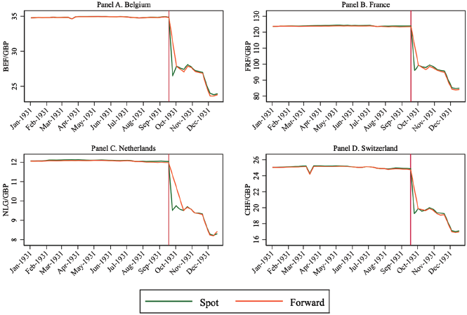
What about the markets? A common measure of expectations of devaluation is the forward premium: the difference between the forward and spot exchange rate. Under a credible peg, the forward premium will fluctuate within a narrow band around zero. For a peg under threat, the premium will plummet. On one hand, studying the franc/pound exchange rate, Accominotti (Reference Accominotti2012) finds that a negative forward premium of up to 0.5 percent opened up from the middle of July due to the fallout of the German Crisis. On the other hand, focusing on the dollar/pound (3-month) forward premium, Eichengreen and Hsieh (Reference Eichengreen, Hsieh, Tilly and Welfens1996, p. 372) conclude that “there is little evidence … [of] a significant perceived probability that sterling would be devalued. As late as the month before the event, it appears, devaluation would have come as a surprise.”
As there is some disagreement in the literature, we analyze a broader basket of currencies and collect the spot, 1-, 2-, and 3-month forward exchange rates for Amsterdam, Brussels, Paris, and Zurich from the “Forward Exchange Rates” section of the Financial Times every Friday.Footnote 9 Belgium, France, the Netherlands, and Switzerland were core to the gold bloc, declaring a joint commitment to the gold standard in 1933 and remaining on until 1936 (Hsieh and Romer Reference Hsieh and Romer2006). As a result, variation in the forward premium should mostly reflect British expectations of devaluation.Footnote 10
Figure 1 plots the (3-month) forward and spot exchange rate, both expressed in foreign currency per British pound, for the four currencies in 1931. The difference between the two is the forward premium. There are three main takeaways. First, the forward premium hovered around zero for much of 1931, suggesting no initial expectations of devaluation.Footnote 11 Second, from August, the premium dropped, ranging between –0.1 percent and –0.5 percent, which could indicate rising expectations of devaluation.Footnote 12 Third, although markets had priced in future depreciation of up to –0.5 percent, the spot price fell by 21–24 percent at the end of September and by 31 percent at the close of the year, suggesting that devaluation at this scale was largely unexpected.Footnote 13
EXCHANGE RATES
Note: The vertical line indicates the break from the gold standard.
Source: Based on data reported in the “Forward Exchange Rates” section of the Financial Times.

How did this substantial and largely unanticipated depreciation affect British industries? Did devaluation benefit exporters over non-exporters? And was it a mean-preserving redistribution between industries, or did devaluation have important aggregate effects? It is to these questions that we now turn.
RESEARCH DESIGN
Data
To identify the causal impact of devaluation on unemployment, we assign treatment and control groups based on an industry’s propensity to export their output. The treatment group consists of export-intensive industries that are sensitive to devaluation owing to their participation in international trade. The control group consists of domestic production or service industries that are less sensitive to devaluation because they are not as exposed to exchange rate shocks. Treatment occurs in September 1931 when Britain switched from a fixed exchange rate under the gold standard to a floating regime.Footnote 14 We therefore require high-frequency data on industry-level unemployment outcomes as well as a measure of export intensity for each industry. Counts of the number of unemployed in 100 industries were published each month in the interwar period by the Ministry of Labour in the Labour Gazette.Footnote 15 These data came from the operation of the national unemployment insurance scheme and therefore include only insured workers. The unemployment insurance scheme in interwar Britain covered most manual workers and some lower-paid non-manual workers.Footnote 16 These data are generally thought to be reliable, having been collected by the interwar British government, and broadly representative despite covering only insured workers. While subsets of these data have been used in many previous studies on interwar unemployment, the complete monthly data were only recently digitized and made available in Paker (Reference Paker2024).
We take the monthly number of workers unemployed in all 100 Labour Gazette industries for the five months before and after the 1931 devaluation: April 1931 to February 1932. We select these dates to provide a balanced pre- and post-treatment window while excluding the period from March 1932, when industry unemployment rates may have been affected by the General Tariff.Footnote 17 While the Ministry of Labour reported the number of unemployed each month in the Labour Gazette, the number of insured workers in each industry was only established once a year in July. We, therefore, linearly interpolate the numbers insured in each industry to achieve a monthly unemployment rate, though we show in our sensitivity analyses that our results are robust to using the July figure in the denominator.
To capture industries’ exposure to devaluation, we collect data from the 1930 Census of Production on the percentage of an industry’s output that was exported. The Final Report on the Fourth Census of Production (1933) was published in five volumes covering 121 industries, including all manufacturing industries, mining, building, and “productive services” of utilities and government. In all industries, firms with fewer than 10 workers were excluded. The reports of most industries contain estimates of the percentage of their production that was exported. This is calculated as total exports divided by total production. These calculations are always reported as a percentage, but in some cases they are calculated with production and exports in terms of value, and in other cases, they are calculated with production and exports in terms of volume. Some industries report multiple products: for example, the saddlery and harness industry reports production and exports for saddlery and harnesses; trunks, bags, and other solid leather goods; fancy goods of leather and artificial leather; and other non-apparel or sporting leather goods (Census of Production, vol. 1, p. 355). In instances like these, when production and exports were reported in terms of value, we totaled exports of all products and production of all products before calculating the percentage exported; when only quantities were provided, we took the export percentage of the primary product.
We matched the industries from the 1930 Census of Production to the Labour Gazette industries according to the mapping provided in Online Appendix Table A1. Three Census of Production industries could not be matched, and many needed to be aggregated to match the Labour Gazette, leaving 75 industries. To aggregate industries, we took an average of the percentage of production exported for the relevant industries, weighted by the number of persons employed in that industry as reported in the Census of Production. In some cases, a Census of Production industry matched multiple Labour Gazette industries, which we aggregated by summing the numbers unemployed and insured.Footnote 18
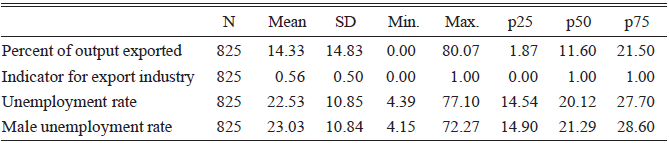
Of the 121 Census of Production industries, exports were not reported in 37 cases. In some cases, this was because the industry was a small subcategory, for example, “Fish Curing,” while in other cases this was because the industry had negligible exports, for example, “Building.”Footnote 19 Our method of aggregation handles these distinctly when both are set to zero. “Fish Curing” becomes part of the larger category “Food Industries Not Separately Specified” when matched to the Labour Gazette, and this zero has no impact on the weighted average. The resulting percentage of output exported for “Food Industries Not Separately Specified” is 5.7 percent, estimated from the subcategories large enough to report exports (Bacon Curing and Sausage; Butter, Cheese, Condensed Milk, and Margarine; Preserved Foods; Sugar and Glucose). In contrast, exports for building remain zero even when combined with public works contracting to match with the Labour Gazette, as both industries had genuinely negligible exports. In the final matched data, ten industries had zero output exported.Footnote 20 Table 1 shows that the average percentage of output exported was 14.3 percent. The industries with the greatest export share were Engineering and Shipbuilding.
SUMMARY STATISTICS

Notes: April 1931–February 1932.
Source: Unemployment rate from the Labour Gazette. Percentage of output exported from the 1930 Census of Production.
Table 1 also shows the wide range of unemployment rates experienced by industries over this period. The average industry-level unemployment rate overall was 22.5 percent. The average unemployment rate was slightly higher when only men were considered, at 23 percent. While the unemployment rate varies monthly, the industries with the highest unemployment rates on average were Shipbuilding; Lead, Tin, Copper, and Iron Mining; and Jute. The industries with the lowest unemployment rates on average were Tramway and Omnibus Service; Gas, Water, and Electricity Supply Industries; and Printing, Publishing, and Bookbinding.
To identify the treatment group, we create a variable, Export i, equal to one if the industry exported more than 10 percent of its production and zero otherwise. We choose this threshold because it is approximately the median. Nearest to this threshold are Dress, Mantle Making, and Millinery and Brush and Broom Making, classified as non-export industries; and Jute and Iron and Steel, classified as export industries, which is consistent with contemporary understanding (see Clay Reference Clay1929, p. 83). We show that our results are not sensitive to the choice of threshold.
This breakdown plausibly creates more and less treated groups. Our main focus is on the impact of devaluation on the export industries, as British exports became more competitive in foreign markets. However, there are countervailing forces that blur the distinction between the export and non-export groups. First, either group may have used imported inputs, which became more expensive after devaluation. This could bias the treatment effect in either direction, depending on which group used more imported inputs. We will revisit this in the next section. Second, the non-export industries may have benefited from depreciation if they competed with imports in the British market. This could bias the treatment effect down. We will return to this later.
The largest export industries were Coal Mining, Engineering, and Cotton Textile manufacturing, while the largest non-export industries were Building, Clothing Production, and Government.Footnote 21
The export-intensive industries had, on average, higher unemployment rates than the non-export industries. In the period before devaluation, from April 1931 through August 1931, the average unemployment rate for the export industries was 25.55 percent, while the average unemployment rate for the non-export industries was 19.42 percent. Despite these differences in average unemployment rates, there are large industries with high unemployment in both groups.Footnote 22 Our measure of export intensity is therefore not simply capturing the largest industries or those with the highest unemployment, even though the average unemployment rate is higher in export industries than in non-export industries.
We also create a variable, Post t, which equals one if the month is after September 1931 and zero otherwise.
Empirical Specification
With all of the key variables constructed, we now turn to the empirical specification. We use a difference-in-differences model with industry and month-year fixed effects to estimate the impact of devaluation on unemployment. Our regression thus takes the form:
where Uit is a measure of the unemployment rate in industry i at time t, Exporti and Postt are as defined previously, αi are industry fixed effects, τt are month-year fixed effects (i.e., fixed effects for April 1931, May 1931, …, February 1932), and X represents a vector of controls. Because our specification uses industry fixed effects, we only need to control for factors that vary within an industry by month. In some specifications, we therefore control for the log of the monthly estimate of the number insured in each industry.
The coefficient of interest is δDD, the estimated average treatment effect on the treated (ATT). δDD captures how unemployment rates for export industries changed with devaluation relative to the change in unemployment rates for non-export industries. Export i * Postt equals one if an industry exported more than 10 percent of its output, and the observation was after September 1931; and zero otherwise.
Identifying Assumptions
Identifying the treatment effect requires parallel trends, no anticipatory effects, and no other major institutional or policy changes that differentially impacted treatment and control groups across the threshold.
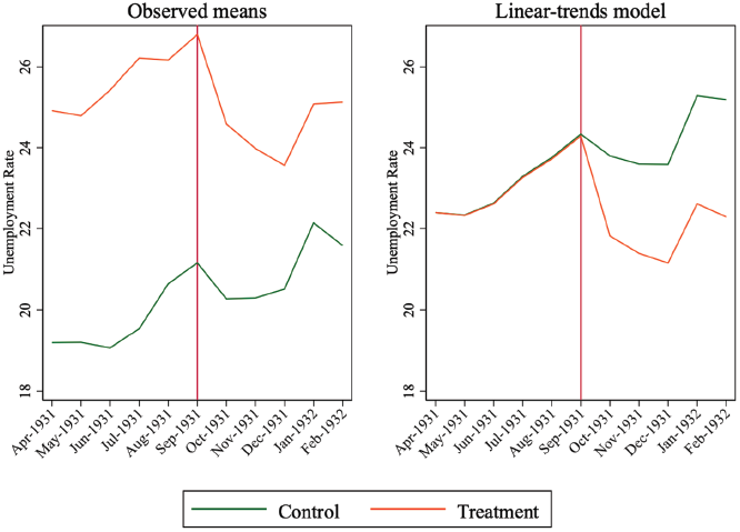
First, we evaluate whether the trends in the unemployment rate are parallel for the control (non-export) and treatment (export) groups before the devaluation date. Figure 2 provides the standard visual checks of this assumption. The left side of the figure plots the mean of the unemployment rate over the whole period for both groups, while the right side gives the results of a linear trends model.Footnote 23 These checks suggest the parallel trends assumption is satisfied. In a hypothesis test of the coefficient on the difference in linear trends prior to treatment, we fail to reject the null hypothesis that the linear trends are parallel, providing additional statistical evidence that this assumption is met (p = 0.8212 for Column (1) of Table 2).
GRAPHICAL DIAGNOSTICS: PARALLEL TRENDS
Notes: Treatment group includes all industries that reported the percent of their output exported in the 1930 Census of Production greater than 10 percent. The vertical line indicates the break from the gold standard.
Sources: Analysis using unemployment data from the Labour Gazette and percent of output exported from the 1930 Census of Production.

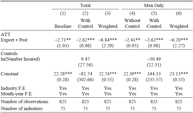
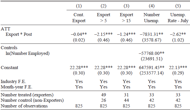
TREATMENT EFFECT OF DEVALUATION ON THE UNEMPLOYMENT RATE

Notes: * p < 0.10, ** p < 0.05, *** p < 0.01. Robust standard errors clustered by industry given in parentheses. Columns (1)–(3) use the total unemployment rate and number insured from the Labour Gazette, while Columns (4)–(6) use the men’s unemployment rate and number insured for men from the Labour Gazette. Export i * Postt equals one if an industry reported the percent of their output exported in the 1930 Census of Production greater than 10 percent and if the month was after September 1931. Columns (3) and (6) weight by the number of insured workers in each industry in August 1931.
Source: Authors’ calculations based on data described in the text.
The recent methodological literature on difference-in-differences has expressed concern that statistical tests for parallel trends in the pre-treatment period, as we just reported, might fail to reject the null hypothesis owing to low power. Following the recommendations in Roth et al. (Reference Roth, Sant’Anna, Bilinski and Poe2023), we conduct a sensitivity analysis of our findings in Table 2 to violations of the parallel trends assumption using the method in Rambachan and Roth (Reference Rambachan and Roth2023), sometimes referred to as “Honest DiD.” This procedure involves calculating confidence intervals for the treatment effect under different assumptions for how much parallel trends could be violated between two consecutive periods. The task is to identify a “breakdown ![]() ,” which indicates how bad the violation of parallel trends would need to be to invalidate a significant result. The sensitivity analysis shows a breakdown value of
,” which indicates how bad the violation of parallel trends would need to be to invalidate a significant result. The sensitivity analysis shows a breakdown value of ![]() , which means that the magnitude of any post-treatment violations of parallel trends would need to be as large as the largest pre-treatment violation in order to invalidate the statistical significance of the result in Column (1) of Table 2. While all of our tests suggest the parallel trends assumption is strongly met, this breakdown value suggests our result is only moderately sensitive to the parallel trends assumption in the first place.
, which means that the magnitude of any post-treatment violations of parallel trends would need to be as large as the largest pre-treatment violation in order to invalidate the statistical significance of the result in Column (1) of Table 2. While all of our tests suggest the parallel trends assumption is strongly met, this breakdown value suggests our result is only moderately sensitive to the parallel trends assumption in the first place.
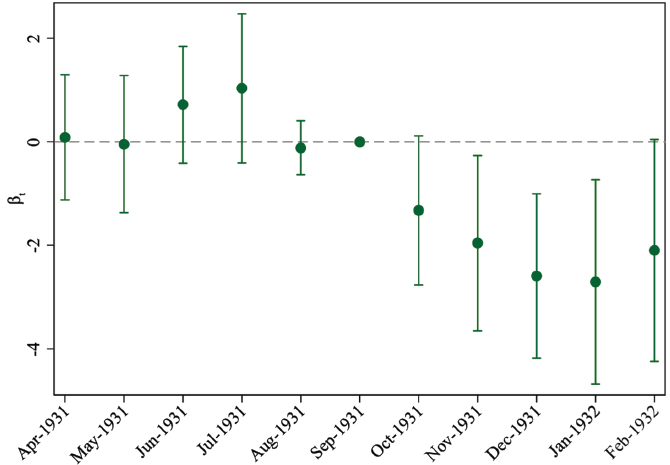
Second, we investigate whether there were anticipatory effects in the standard way by conducting a test in the spirit of Granger causality, which fails to reject the null hypothesis of no anticipatory effects (p = 0.5671 for Column (1) of Table 2). This indicates that our model does not suffer from anticipation. We can also consider pre-period and post-period treatment effects in an event study plot, presented in Figure 3. To do so, we consider alternative treatment dates five months either side of September 1931. The point estimates show the change in the unemployment differential between export and non-export industries for the alternative treatment dates. The bars indicate the 90 percent confidence interval. Prior to treatment, there are no significant differences in the trend between the treatment group of export industries and the control group of non-export industries. After the treatment, a significant difference emerges, with the unemployment rate falling more for export industries than for non-export industries.Footnote 24
GRAPHICAL DIAGNOSTICS: NO ANTICIPATION
Notes: Treatment group includes all industries that reported the percent of their output exported in the 1930 Census of Production greater than 10 percent. Treatment occurred in September 1931. Ninety percent confidence intervals reported.
Sources: Analysis using unemployment data from the Labour Gazette and percent of output exported from the 1930 Census of Production.

Third, we are concerned about other possible policy changes that occurred around the treatment date that may have impacted the treatment and control groups differently. One such policy change was the Anomalies Act, enforced from October 1931. This Act disproportionately affected women, making it difficult for married women to receive unemployment benefits. This may have impacted the unemployment of women around the time of our treatment, and women were more likely to be in export industries than in non-export industries. To avoid any confounding from the Anomalies Act, we present our results for the fully insured population (including women) and for only men, who were less impacted by the Anomalies Act.
Another possible policy change was protection as several imported goods received higher tariffs in the second budget of 1931 (Hansard 1931a, cols. 297–312).Footnote 25 As a result, we exclude the newly-protected industries in a robustness exercise.
RESULTS
Table 2 presents the main results.Footnote 26 The average treatment effect is given by the coefficient on Export i * Postt, which is the difference in the change in unemployment rates before and after devaluation between the treated and the control groups. Recall that the treated group contains the export industries, exposed to devaluation, while the control group consists of the industries that exported less or not at all. The first three columns in Table 2 use the total unemployment rate as the outcome variable, including men and women, while the last three columns use the men’s unemployment rate to avoid confounding from the 1931 Anomalies Act.Footnote 27
Focusing on Column (1), which gives the baseline results for the total unemployment rate, the estimate of −2.71 indicates that devaluation lowered unemployment rates by 2.71 percentage points more for export industries relative to the non-export control group. This estimate is statistically significant at the 5 percent level and is economically meaningful. Prior to devaluation, the unemployment rate was 6.1 percentage points higher for the export industries than for the non-export industries on average. Devaluation, therefore, almost halved the difference in the unemployment rate between the export and non-export industries.
Column (2) shows that the treatment effect is just slightly smaller at −2.62 (p < 0.01) when controlling for the average number of insured workers in the industry. Column (3) weights the model by the number of insured workers in each industry in August 1931. Weighting corrects for the over-representation of industries with a small number of workers in the unweighted regressions that treat all industries as equally important. The estimated average treatment effect is greater at −6.84 (p < 0.01). This suggests that the finding that devaluation advantaged export industries relative to non-export industries is especially true for the industries that had a larger share of workers in the labor force. The weighted treatment effect can be taken as an approximate population-level impact of devaluation on unemployment. We focus in the rest of this section on the more conservative unweighted estimates, but we consider the implications of this weighted estimate on the aggregate impact.
Columns (4), (5), and (6) give the estimates for men’s unemployment rates from a model similar to the baseline, with an industry size control, and weighted by industry size. In general, the estimates are broadly in line with the estimates for total unemployment and are still strongly statistically significant. The estimates are slightly smaller, suggesting that there may indeed have been differences in changes in industry unemployment rates during this period for men and women.
Table 3 explores the robustness of our baseline results to different definitions of export industries and to different measures of unemployment. The first column uses percent of output exported as a continuous measure, while Columns (2) and (3) experiment with thresholds of 5 percent and 15 percent for determining export vs. non-export industries. Because of the asymmetric and often small number of clusters in the treated or control groups in these models, the standard errors are robust but not clustered, so they should be interpreted cautiously. Focusing first on Column (1), the result indicates that a 1 percentage point increase in the share of output exported is associated with a 0.04 percentage point decline in the unemployment rate after devaluation. From Table 1, the standard deviation of the percent of output exported is 14.84; this means that a one standard deviation increase is associated with a 0.59 percentage point decrease in the unemployment rate. Columns (2) and (3) show that the effect size is consistent, though slightly smaller, when a more or less conservative threshold for identifying export industries is used.
ROBUSTNESS TO DIFFERENT MEASURES OF EXPORT AND UNEMPLOYMENT

Notes: * p < 0.10, ** p < 0.05, *** p < 0.01. Robust standard errors given in parentheses. Column (1) uses the continuous export share. Export i equals one if an industry reported the percent of their output exported in the 1930 Census of Production greater than 5 percent or 15 percent in Columns (2) and (3), respectively. Column (4) uses the total number unemployed as the dependent variable, while Column (5) uses the overall unemployment rate where the denominator is the number insured in July.
Source: Authors’ calculations based on data described in the text.
Table 3 also explores the robustness of the findings to changes in the outcome measure. Column (4) uses the number unemployed as the outcome, controlling for the log number employed. Column (5) uses the unemployment rate with the raw number of insured in the industry in July as the denominator rather than the linearly interpolated value. The findings confirm the baseline results in Table 2, Column (1).
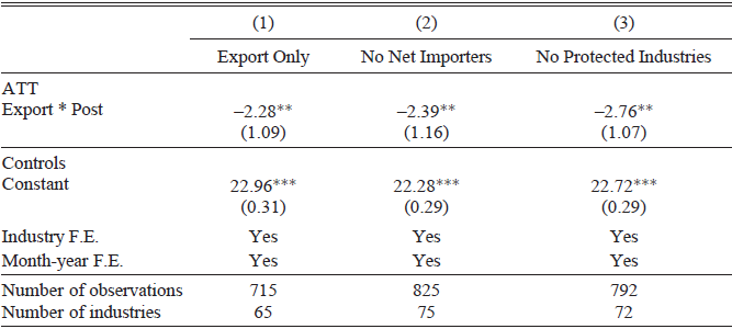
Table 4 considers the robustness of the findings to different samples. Column (1) calculates the effects on the intensive margin of exporting by excluding 10 industries with no reported exports in the Census of Production. The effect sizes are similar to the baseline model.
ROBUSTNESS TO DIFFERENT SAMPLES

Notes: * p < 0.10, ** p < 0.05, *** p < 0.01. Robust standard errors clustered by industry given in parentheses. Column (1) restricts the sample to only industries with non-zero exports, where Export i * Post t equals one if an industry reported the percent of their output exported in the 1930 Census of Production greater than 10 percent and if the month was after September 1931. Column (2) re-classifies 13 industries as non-exporters which were indicated net importers in Barna (Reference Barna1952). Column (3) uses the baseline measure of an exporter but drops protected industries from the sample.
Source: Authors’ calculations based on data described in the text.
As devaluation lowers the price of an industry’s output in foreign markets but also raises the price of imported inputs, an alternative treatment indicator could be based on net exports. This information is not readily available in the Census of Production. To gauge the importance of this issue, we use the calculations in Barna (Reference Barna1952) of import and export intensity for 36 industries in 1935 to recode export industries from 1 to 0 if the import share was greater than the export share (indicating that they were net importers). Unfortunately, this information is only available for a coarser set of industries and well after devaluation, when import and export intensity is likely to have swung toward the latter following the drop in the exchange rate. Keeping these limitations in mind, we recode 13 of our 42 export industries to non-export industries based on the classifications in Barna (Reference Barna1952, p. 57).Footnote 28 Column (2) shows that, with this revised export measure, the treatment effect is slightly smaller but remains economically and statistically significant.
We also considered whether non-export industries may have been exposed to treatment from devaluation through the increased costs of imports. The data from Barna (Reference Barna1952) indicate that non-export industries had a relatively low import share, which suggests that the control group was largely sheltered from the devaluation.
Finally, Column (3) drops three industries that received protection during this period, which we identified using primary sources, to ensure that they do not confound the results (House of Commons Parliamentary Papers 1938, pp. 208–15).Footnote 29 Again, the results confirm the baseline estimates given in Table 2, although the treatment effect is slightly larger.
In Online Appendix Tables A3 and A4, we present the results of the robustness checks in Tables 3 and 4 for men only. In Online Appendix Table A6, we show that the results are robust to using seasonally-adjusted unemployment rates, and we present the results of placebo tests indicating that seasonal patterns are not driving our results. Online Appendix Table A7 confirms that the results are not driven by differences in the volatility of the unemployment rate between export and non-export industries. When we drop the most volatile export industries and the least volatile non-export industries from our difference-in-differences model, measured in different ways, the results are strengthened. Online Appendix Table A8 displays the results of further robustness checks, where the cyclical sensitivity of each industry is captured by a regression of changes in the unemployment rate on GDP growth at a monthly frequency between July 1924 and July 1936. When we drop the most cyclical export industries and the least cyclical non-export industries from our difference-in-differences model, the results are robust. Online Appendix Table A9 shows that our results are not sensitive to increasing or decreasing the number of months after devaluation included in the analysis. All of the robustness checks confirm that devaluation caused an economically and statistically significant decrease in unemployment rates in export industries relative to non-export industries.
AGGREGATE IMPACT
How did devaluation affect the recovery from the Great Depression? Following a number of other historical studies (Hausman Reference Hausman2016; Hausman, Rhode, and Wieland Reference Hausman, Rhode and Wieland2019; Chadha et al. Reference Chadha, Lennard, Solomou, Thomas, Clavin, Corsetti, Obstfeld and Tooze2023), we go from micro to macro using our estimated treatment effect and some counterfactual simulations. This exercise has three key features. First, it isolates the export channel of devaluation but does not include other channels—such as expectations, uncertainty, and monetary policy—because these aggregate factors are “differenced out” in Equation (1) (Nakamura and Steinsson Reference Nakamura and Steinsson2014). Focusing on one channel is desirable for studying counterfactuals, as one element varies while others are fixed. Second, it accounts for the size and share of the industries in the treatment and control groups. Third, it allows for possible general equilibrium effects as the relative impact is not necessarily equal to the aggregate (Ramey Reference Ramey2011; Orchard, Ramey, and Wieland Reference Orchard, Ramey and Wieland2023).
The first step is to define the actual and counterfactual unemployment rate for each industry. Using potential outcomes, the industry-level unemployment rate with devaluation is:
The counterfactual industry-level unemployment rate without devaluation is:
The difference between the actual and counterfactual is δ DDExport i * Post t. To calculate the aggregate impact, we weight by an industry’s share of total employment, which accounts for an industry’s contribution to the aggregate unemployment rate, and sum over all industries:

where Lt is the labor force, given by the number of insured workers and φt is the change in the aggregate unemployment rate due to devaluation. This setup implies that devaluation has the same effect, δDD, for all export industries. To give a sense of magnitudes, we calculate the aggregate unemployment rate as ![]() and the counterfactual aggregate unemployment rate as
and the counterfactual aggregate unemployment rate as ![]() .
.
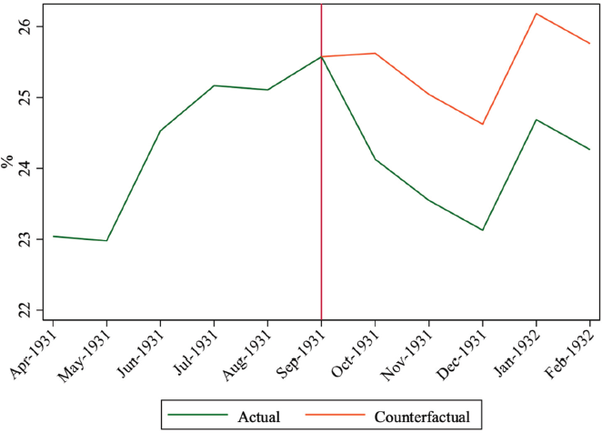
Figure 4 plots the actual and counterfactual unemployment rate based on the treatment effect presented in Column (1) of Table 2 of −2.71.Footnote 30 With devaluation, the actual unemployment rate declined from 25.5 percent in September to 23.1 percent in December 1931. Without devaluation, the counterfactual unemployment rate would have been sticky around 25 percent, creeping down to 24.6 percent by the end of 1931. Therefore, the impact of devaluation on exporters lowered the aggregate unemployment rate by approximately 1.5 percentage points (shown by the distance between the two lines in Figure 4).
ACTUAL AND COUNTERFACTUAL UNEMPLOYMENT
Notes: The vertical line indicates the break from the gold standard.
Source: Authors’ calculations based on data described in the text.

Our estimate of the treatment effect, δDD, tells us how export industries performed relative to non-export industries. However, the micro and macro effects may not be equal (Ramey Reference Ramey2011; Orchard et al. Reference Orchard, Ramey and Wieland2023). The aggregate impact could be smaller if there are negative spillovers, such as if a job gained in one industry is a job foregone in another, which might hold in a tight labor market. The aggregate impact could be larger if there are positive externalities, such as if the reduction in unemployment for exporters due to devaluation also reduces unemployment for non-exporters, albeit disproportionately, or devaluation stimulates non-export industries that compete with imports.
To allow for general equilibrium effects, we can augment Equation (2) with λ, which attenuates, amplifies, or holds constant the treatment effect:

We consider three values of λ. The first is λ = 1, which is the baseline case. The second is λ = 0.5, which dampens the treatment effect by half. The third is λ = 2, which doubles the treatment effect. The results are shown in Online Appendix Figure A4. As expected, assuming negative spillovers, λ = 0.5 halves the aggregate impact; assuming positive spillovers, λ = 2 doubles the aggregate impact, and so on.
On balance, our sense is that the baseline is most realistic. On λ < 1, it is difficult to identify a credible mechanism through which job creation in the export industries led to job destruction in the non-export industries. On λ > 1, it is quite possible that more jobs and incomes in the export industries raised demand in the non-tradable sector. For example, building was the biggest employer among the non-export industries. It is plausible that stimulus to the export industries boosted the building of homes and factories for its workers and firms. Other big non-export industries provided staples (such as food, drink, and clothing) and services (such as transport and utilities). However, a large λ results in rising counterfactual unemployment, which is possibly a stretch given that the unemployment rate was already so high.Footnote 31
In the context of very high unemployment, a reduction of 1.5 percentage points is relatively modest, but it is meaningful in absolute terms, translating to about 140,000 fewer people out of work.Footnote 32 A useful reference point is Keynes and Henderson’s proposal to increase government spending by £100m per annum for three years. Dimsdale and Horsewood (Reference Dimsdale and Horsewood1995) estimate that this stimulus package would have raised employment by 111,000–120,000 in the first year, rising to a peak of 303,000–330,000 by the third year, depending on assumptions about interest rates and crowding out. Crafts and Mills (Reference Crafts and Mills2013), based on a government expenditure multiplier of 0.8, calculate an upper bound of 200,000 fewer unemployed. Therefore, the two policies have similar employment benefits in the short run.
This drop in aggregate unemployment would have also had a positive impact on the dismal fiscal arithmetic for the Treasury. With benefit rates of 13s. 6d. for women and 15s. 3d. for men per week from 8 October 1931 (Burns Reference Burns1941, p. 368), this saved roughly £93,000 a week in benefit payments if we assume that all of the jobs went to women, or £105,000 a week if all of the jobs went to men. This is equivalent to 0.6 percent and 0.7 percent of weekly government spending (Mitchell Reference Mitchell1988).Footnote 33
Another way to measure the aggregate impact is to convert from jobs to output using Okun’s law, which is an empirical regularity that holds between the change in the unemployment rate and the growth of GDP (see, e.g., Paker Reference Paker2023).Footnote 34 Online Appendix Figure A5 displays a robust negative relationship for interwar Britain across three different samples. The slope, which is the estimated Okun’s coefficient, is −0.4 (t = −5.6) for the long pre-treatment window, 1920:2–1931:9, −0.6 (t = −6.9) for the gold standard era, 1925:4–1931:9, and −0.5 (t = −7.4) for the full interwar period, 1920:2–1938:12.Footnote 35 Using the lower estimate translates to a one-off jump in GDP growth of 0.6 percentage points; using the upper estimate raises the impact to 0.9 percentage points. As a temporary increase in the growth rate permanently raises the level, these bounds represent a non-trivial contribution to the shoots of economic recovery, especially when we consider that this captures only one channel of devaluation and excludes other potential mechanisms.Footnote 36
An interesting question is whether the stimulus to the export industries from devaluation was due to higher quantities or prices. To gain some insight, we investigate the response of aggregate trade flows using quarterly figures collected from The Economist (1933, p. 234). Relative to the second quarter of 1931, the volume of exports increased by 0.5 percent in the third quarter, by 8.1 percent in the fourth quarter, and by 3.9 percent in the first quarter of 1932. The price of exports, however, fell quarter by quarter, dropping by 7.3 percent over that interval as part of the global slump in commodity prices. This suggests that exporters benefited from higher demand, as opposed to higher prices, which is consistent with the job creation we find.
CONCLUSION
Britain’s suspension of the gold standard in 1931 has been described as “one of the most shocking policy shifts in the history of the global economy” (Morrison Reference Morrison2016, p. 176). This sweeping reform had multiple potential effects: it was a turn in the macroeconomic trilemma that released monetary policy to pursue new objectives, it was a regime change that shifted expectations, and it was a depreciation that improved international competitiveness. In classic accounts, releasing the “golden fetters” is regarded as a pre-requisite of the U.K.’s recovery from the Great Depression (Solomou Reference Solomou1996; Morys Reference Morys, Floud, Humphries and Johnson2014; Crafts Reference Crafts2018), and contemporary observers such as Keynes certainly regarded it as such (Keynes 2013a, pp. 245–49).
However, there is space for new empirical work that distinguishes between these complementary channels. In this paper, we focus on the export channel, using quasi-experimental methods to capture how devaluation affected export and non-export industries. Our analysis relies on a newly-constructed monthly dataset for 75 industries collected from the Labour Gazette and Census of Production.
We find that unemployment rates evolved in parallel before devaluation but diverged after. Unemployment rates fell by 2.71 percentage points more in export-intensive industries relative to non-export industries. This result, which is robust to many alternative specifications, is also large in magnitude. The export industries experienced higher unemployment rates than the non-export industries prior to devaluation. Leaving the gold standard reduced this difference by almost 50 percent, bringing labor market outcomes for workers in export and non-export industries into closer alignment.
This improvement in the unemployment rate for export industries after devaluation was not a zero-sum game. The jobs created in the export industries were not offset by jobs lost in the non-export industries. According to our counterfactual simulations, our conservative estimates suggest the export channel of devaluation lowered the aggregate unemployment rate by 1.5 percentage points—equivalent to approximately 140,000 fewer people out of work. Through the reduction of unemployment benefit payments alone, this resulted in savings for the Treasury of 0.6–0.7 percent of spending per week. Based on our estimates of Okun’s law, we project that this reduction in the aggregate unemployment rate led to a jump in GDP growth of 0.6 to 0.9 percentage points.
When the persistent unemployment of the 1920s collided with the Great Depression, a series of offsetting shocks were required to reverse the vortex of falling output and prices. The evidence we have provided in this paper indicates that devaluation, through the export channel alone, gave an almost immediate boost to export industries. This policy shift improved the employment situation, the fiscal position, and economic activity. Therefore, the stimulus of devaluation to the export industries was an important initial spark in Britain’s economic recovery from the Great Depression. Other channels, such as cheap money and rearmament, reinforced and completed this recovery. While the U.K. experience is interesting in its own right, this also adds important context to the international pattern of devaluation and recovery from the Great Depression so familiar to economic historians.


 Open access