


1. Introduction
The flow of a shallow layer of granular materials over an erodible bed, composed of the same material referred to as a surface flow, is of importance in industrial processes related to storage, transportation and handling of particles. The knowledge of surface granular flows also aids in answering questions related to natural processes such as the flow of sand dunes, avalanches, landslides and pyroclastic flows. In such surface flows, the flowing layer of particles can either erode the heap or deposit particles on it. Bouchaud et al. (Reference Bouchaud, Cates, Prakash and Edwards1994) proposed that the erosion rate, $\Gamma$
, should depend on the difference between the inclination of the free surface of the heap during flow (given by an angle
$\Gamma$
, should depend on the difference between the inclination of the free surface of the heap during flow (given by an angle $\beta$
) and the inclination of the free surface when there is no erosion or deposition, defined by the neutral angle,
$\beta$
) and the inclination of the free surface when there is no erosion or deposition, defined by the neutral angle, $\beta _n$
, as
$\beta _n$
, as
 \begin{equation} \Gamma = \gamma \delta (\beta - \beta _n). \end{equation}
Here, $\Gamma$
is the rate of erosion (
$\Gamma$
is the rate of erosion ( $\Gamma \gt 0$
) or deposition (
$\Gamma \gt 0$
) or deposition ( $\Gamma \lt 0$
) of particles from the heap,
$\Gamma \lt 0$
) of particles from the heap, $\gamma$
is a proportionality constant and
$\gamma$
is a proportionality constant and $\delta$
is the thickness of the flowing layer. For instances where the flowing layer is relatively thick
$\delta$
is the thickness of the flowing layer. For instances where the flowing layer is relatively thick $(\delta \gt 30d$
, where
$(\delta \gt 30d$
, where $d$
is the particle diameter), Boutreux et al. (Reference Boutreux, Raphaël and de Gennes1998) proposed that the erosion rate is independent of the flowing layer thickness,
$d$
is the particle diameter), Boutreux et al. (Reference Boutreux, Raphaël and de Gennes1998) proposed that the erosion rate is independent of the flowing layer thickness, $\delta$
, and depends only on the difference between the free surface angle and the neutral angle as
$\delta$
, and depends only on the difference between the free surface angle and the neutral angle as
 \begin{equation} \Gamma = V(\beta - \beta _n). \end{equation}
Here, $V$
is a characteristic velocity of the order of
$V$
is a characteristic velocity of the order of $\sqrt {gd}$
. At steady state (
$\sqrt {gd}$
. At steady state ( $\Gamma = 0$
), both models yield
$\Gamma = 0$
), both models yield $\beta =\beta _n$
, i.e., the surface angle (
$\beta =\beta _n$
, i.e., the surface angle ( $\beta$
) is equal to the neutral angle (
$\beta$
) is equal to the neutral angle ( $\beta _n$
). Douady et al. (Reference Douady, Andreotti and Daerr1999) and Khakhar et al. (Reference Khakhar, Orpe, Andresen and Ottino2001) derived similar expressions for the erosion rate using depth-averaged mass and momentum equations with different closure assumptions.
$\beta _n$
). Douady et al. (Reference Douady, Andreotti and Daerr1999) and Khakhar et al. (Reference Khakhar, Orpe, Andresen and Ottino2001) derived similar expressions for the erosion rate using depth-averaged mass and momentum equations with different closure assumptions.
Several experimental studies on surface flow over heaps have been performed in the last three decades. For surface flow over heaps in quasi-two-dimensional systems bounded by frictional side walls, it was shown by Khakhar et al. (Reference Khakhar, Orpe, Andresen and Ottino2001) that the flowing layer thickness varies as the square root of the mass flow rate, the shear rate is nearly constant in the flowing layer and the surface angle increases with mass flow rate. Komatsu et al. (Reference Komatsu, Inagaki, Nakagawa and Nasuno2001) and Richard et al. (Reference Richard, Valance, Métayer, Sanchez, Crassous, Louge and Delannay2008) showed that the flow does not stop abruptly at the base of the flowing layer, but continues to creep exponentially slowly inside the erodible bed, i.e. the boundary between the flow–no flow zone is diffuse. This exponential creep was attributed to the wall–particle interactions and non-locality in the interactions by Martínez et al. (Reference Martínez, González-Lezcano, Batista-Leyva and Altshuler2016). Taberlet et al. (Reference Taberlet, Richard, Valance, Losert, Pasini, Jenkins and Delannay2003) showed that the friction at the side walls significantly affects the inclination of the free surface of the heaps. This was further emphasised by Jop et al. (Reference Jop, Forterre and Pouliquen2005, Reference Jop, Forterre and Pouliquen2006) in their experiments, where they varied the distance between the side walls from 19 particle diameters to 570 particle diameters. They found that merely increasing the distance between the end walls does not eliminate the wall effects. In fact, for the channel with the narrowest width, a plug flow zone was observed near the centre of the channel, which disappeared as the channel width was increased. Also, as the channel widths were increased, the flows became slower, the flowing layer thicknesses increased and the shear rates also varied by a factor of approximately 10. Numerical confirmation of these results was provided by de Ryck et al. (Reference de Ryck, Zhu, Wu, Yu and Zulli2010) for flows over both ‘frozen’ and ‘non-frozen’ beds. Katsuragi et al. (Reference Katsuragi, Abate and Durian2010) used speckle visibility spectroscopy on quasi-two-dimensional bounded heaps and proposed that the depth below the free surface of a heap may be considered an order parameter that influences jamming as well as dynamical heterogeneities. Fan et al. (Reference Fan, Umbanhowar, Ottino and Lueptow2013, Reference Fan, Jacob, Freireich and Lueptow2017) showed that the streamwise velocity profiles for surface flows in bounded heap flows decay linearly with depth inside the flowing layer and these profiles are self-similar. Fully three-dimensional flow fields in conical wedge-shaped heaps were considered by Isner et al. (Reference Isner, Umbanhowar, Ottino and Lueptow2020a , Reference Isner, Umbanhowar, Ottino and Lueptow b ) and were shown to follow the JFP scaling (Jop et al. Reference Jop, Forterre and Pouliquen2005).
All the studies mentioned above are in heaps with frictional side walls. A few experimental studies are reported where the frictional side walls are absent and the heap is fully three-dimensional. Studies on the mechanisms of growth of conical heaps formed by pouring sand on a finite sized circular disc have been reported by Altshuler et al. (Reference Altshuler, Ramos, Martínez, Batista-Leyva, Rivera and Bassler2003, Reference Altshuler, Toussaint, Martínez, Sotolongo-Costa, Schmittbuhl and Måløy2008). An experimental study on the formation and dynamics of fully three-dimensional conical heaps in the absence of side wall effects was performed by Mandal & Khakhar (Reference Mandal and Khakhar2019). For steady surface flows on these asymmetric conical heaps, the neutral angle was found to remain constant over a three-fold increase in mass flow rate and was less than the angles of repose by approximately $10^\circ$
. The streamwise velocity profiles could be described by Gaussian functions and were found to decrease downstream along the heap, accompanied by a corresponding decrease in flowing layer thickness, due to an increase in the width of the flowing zone downstream.
$10^\circ$
. The streamwise velocity profiles could be described by Gaussian functions and were found to decrease downstream along the heap, accompanied by a corresponding decrease in flowing layer thickness, due to an increase in the width of the flowing zone downstream.
In this study, we consider a fully developed surface flow at steady state on a three-dimensional heap, formed by pouring granular particles from a wedge-shaped hopper with a slit exit, on a rough base, which has a single wall on its back edge. A steady surface flow is established when the edge of the heap reaches the front end of the base, as shown in figure 1. The central region of the heap surface is planar and the flow is uni-directional in this region. The system is an example of typical three-dimensional heaps encountered in practice and surface flows in natural systems, but has not been studied in detail yet. In this work, we measure surface velocities using high-speed videography and image analysis, measure the angles at the free surface, and obtain estimates of flowing layer thickness. The objective is to gain insights into the behaviour of steady, fully developed surface flows on fully three-dimensional heaps in the absence of side wall effects. The paper is organised as follows: experimental details are given in § 2, results are presented in § 3 followed by conclusions in § 4.
An image of the steady surface flow of granular materials on the surface of a three-dimensional heap. The coordinate system is shown along with vectors showing the pattern of the flow.

2. Experimental details
2.1. System
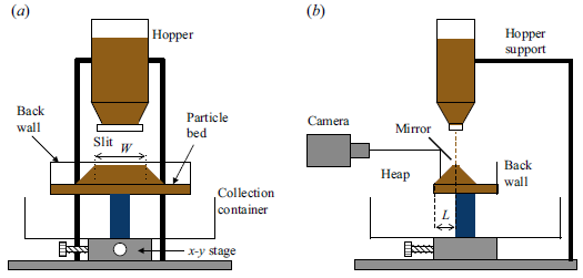
A schematic representation of the experimental set-up with different parts labelled: (a) front view and (b) side view.

A schematic view of the experimental set-up is shown in figure 2. A hopper with a rectangular cross-section and a converging lower section, of capacity 1400 cm $^3$
, is suspended above a rectangular plate of dimensions 40 cm
$^3$
, is suspended above a rectangular plate of dimensions 40 cm $\times$
20 cm, with the help of two rods attached to the base. Slits of length 10 cm, at the throat of the hopper, are interchangeable, and four different slits of depths 3 mm, 5 mm, 7 mm and 9 mm are used to yield different mass flow rates. The rectangular plate has a lip of height 10 mm at its edges, enabling the formation of a rough base of particles and a single wall of height 10 cm at its back edge prevents particles from falling off the plate from the rear. There are no other walls at the front or side edges of the plate. The plate is fixed above a cylindrical container to collect the particles which spill over the edges of the plate. Forward and sideways movement of the plate, relative to the hopper, is possible with the help of two screws.
$\times$
20 cm, with the help of two rods attached to the base. Slits of length 10 cm, at the throat of the hopper, are interchangeable, and four different slits of depths 3 mm, 5 mm, 7 mm and 9 mm are used to yield different mass flow rates. The rectangular plate has a lip of height 10 mm at its edges, enabling the formation of a rough base of particles and a single wall of height 10 cm at its back edge prevents particles from falling off the plate from the rear. There are no other walls at the front or side edges of the plate. The plate is fixed above a cylindrical container to collect the particles which spill over the edges of the plate. Forward and sideways movement of the plate, relative to the hopper, is possible with the help of two screws.
Experiments were performed using monodisperse spherical stainless steel balls ( $d=0.110 \pm 0.008\,\rm cm$
) and nearly sphere glass beads of two different sizes (
$d=0.110 \pm 0.008\,\rm cm$
) and nearly sphere glass beads of two different sizes ( $d=0.103 \pm 0.0096\,\rm cm$
and
$d=0.103 \pm 0.0096\,\rm cm$
and $d=0.165 \pm 0.011\,\rm cm$
). The density of the steels balls is
$d=0.165 \pm 0.011\,\rm cm$
). The density of the steels balls is $\rho _p=7.5$
gcm
$\rho _p=7.5$
gcm $^-{^3}$
and of the glass beads, it is
$^-{^3}$
and of the glass beads, it is $\rho _p=2.5$
gcm
$\rho _p=2.5$
gcm $^-{^3}$
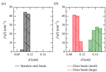
. The size distributions of the beads, obtained by image analysis of photographs of well-separated beads on a white surface, are given in figures 3(a) and 3(b). The sample size is 3137 particles for 1 mm steel beads, 3245 particles for the 1 mm glass beads and 821 particles for the 1.7 mm glass beads. The glass beads are made from red glass so as to make them reflective, which helps in their detection during image analysis. The steel beads are reflective.
$^-{^3}$
. The size distributions of the beads, obtained by image analysis of photographs of well-separated beads on a white surface, are given in figures 3(a) and 3(b). The sample size is 3137 particles for 1 mm steel beads, 3245 particles for the 1 mm glass beads and 821 particles for the 1.7 mm glass beads. The glass beads are made from red glass so as to make them reflective, which helps in their detection during image analysis. The steel beads are reflective.
Number fraction distributions of particle diameter for (a) stainless steel and (b) glass beads.

2.2. Experimental methods
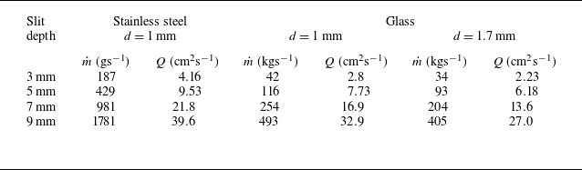
The slits are calibrated by measuring the weight of the beads collected over a fixed duration of time to obtain the mass flow rate, $\dot {m}$
, for each slit for a given material. The mass flow rates for the four slits are given in table 1 for each of the beads. The volumetric flow rate per unit width of the slit,
$\dot {m}$
, for each slit for a given material. The mass flow rates for the four slits are given in table 1 for each of the beads. The volumetric flow rate per unit width of the slit, $Q$
, is defined as
$Q$
, is defined as $\dot {m}/\rho _b w$
, where
$\dot {m}/\rho _b w$
, where $\rho _b$
is the bulk density of the material and
$\rho _b$
is the bulk density of the material and $w=10$
cm is the width of the slit. The bulk density in each case is obtained as
$w=10$
cm is the width of the slit. The bulk density in each case is obtained as $\rho _b=\rho _p\phi$
, where
$\rho _b=\rho _p\phi$
, where $\phi$
is the solid volume fraction in the flowing layer. We take
$\phi$
is the solid volume fraction in the flowing layer. We take $\phi =0.6$
based on simulation results for a similar system (Ray & Khakhar Reference Ray and Khakhar2021). The values of
$\phi =0.6$
based on simulation results for a similar system (Ray & Khakhar Reference Ray and Khakhar2021). The values of $Q$
for the corresponding mass flow rates are also given in table 1.
$Q$
for the corresponding mass flow rates are also given in table 1.
Mass flow rates ( $\dot {m}$
) and volumetric flow rates per unit width (
$\dot {m}$
) and volumetric flow rates per unit width ( $Q$
) for the different slits and beads.
$Q$
) for the different slits and beads.

The position of the rectangular plate is so adjusted that the distance between the pouring point and the front edge of the plate ( $L$
) is 8 cm. The pouring height, which is the distance between the slit and the surface of the rough bed, is kept at 9 cm for all the experiments. The resulting heap is large enough and the flowing layer is sufficiently thick to study the surface flow at steady state on the heap surface. A bed of granular materials of height the same as the height of the lip is prepared before the start of the experiments, and this serves as a rough base on which the heap is formed and surface flow is established.
$L$
) is 8 cm. The pouring height, which is the distance between the slit and the surface of the rough bed, is kept at 9 cm for all the experiments. The resulting heap is large enough and the flowing layer is sufficiently thick to study the surface flow at steady state on the heap surface. A bed of granular materials of height the same as the height of the lip is prepared before the start of the experiments, and this serves as a rough base on which the heap is formed and surface flow is established.
The flow is initiated by opening the slit of the hopper, which was previously filled with the material. The material starts to deposit, and the heap grows until the leading edge of the heap reaches the front edge of the plate and a steady surface flow is established, as shown in figure 1 . The pouring is now stopped and a light-emitting diode (LED) light is focused on the heap from the front to illuminate the particles on the heap. A mirror is positioned at an angle to the free surface of the heap so as to capture the reflection of the bright spots on the illuminated particles at the surface of the heap, as shown in figure 2(b). A high-speed camera is used (Photron FASTCAM SA3 with a ZOOM-Nikkor 24–85 mm lens), with its axis horizontal and the mirror is adjusted to capture images of the surface flow on the heap. A sheet of mm scale graph paper is now carefully placed on the visible surface of the heap and a still photograph of its reflection in the mirror is taken. This image is used to obtain the scale for converting from pixels to distance units during image analysis.
The pouring is then initiated again and video recording of the steady surface flow is started after an initial transient flow period, found to be approximately 6 s. The videos are recorded at $500$
frames per second and a resolution of
$500$
frames per second and a resolution of $1024 \times 768$
pixels until the hopper is empty. The frames are saved as images, and image analysis is done for
$1024 \times 768$
pixels until the hopper is empty. The frames are saved as images, and image analysis is done for $1000$
frames to obtain the positions and velocities of each particle in the region of interest in each frame. The image analysis methodology is described in more detail in the next section. The experiments are repeated five times for each flow rate and for each of the three particles used.
$1000$
frames to obtain the positions and velocities of each particle in the region of interest in each frame. The image analysis methodology is described in more detail in the next section. The experiments are repeated five times for each flow rate and for each of the three particles used.
To measure the angle of the heap free surface, both during surface flow and when the flow is stopped, a laser beam is pointed at the central region of the heap and videos are taken from the side. The vertical direction is obtained using a plumb line and the angles are measured, with respect to this vertical line using ImageJ software, close to the laser spot. The central region of the heap surface during flow was found to be planar in the images taken from the side.
(a) Uncoated metal blade before insertion into the flowing layer and (b) soot-coated metal blade after removal from the flow. The dashed lines demarcate the region where soot has been eroded by the flowing layer.

For measurement of the flowing layer thickness, a weakly intrusive method, similar to that used by Jop et al. (Reference Jop, Forterre and Pouliquen2005) and Mandal & Khakhar (Reference Mandal and Khakhar2019), is used. A metal blade of width 1.8 cm and thickness 0.3 mm is coated on both sides with soot in the flame of a candle and dipped in the central region of the heap for the duration of the flow (5–15 s depending on the slit used). The soot is eroded by the flowing layer, as shown in figure 4. The experiment is repeated three times, yielding three blades. Each side of each blade is illuminated by a high intensity light source and an image of the blade is taken. This image is thresholded appropriately in ImageJ so that the eroded region is white and all the sooty regions are black, yielding a sharp demarcation of the flowing region. The length of the region, where the soot has been eroded by the flowing layer (figure 4
b), is measured using ImageJ near the central region of the blade. This length is taken to be a measure of the flowing layer thickness, $\delta$
. The method resulted in consistent results over the six measurements of
$\delta$
. The method resulted in consistent results over the six measurements of $\delta$
carried out for each case.
$\delta$
carried out for each case.
A few experiments are also conducted by varying the distance of the pouring point from the front edge of the plate (marked as $L$
in figure 2
b) to 10 cm and 14 cm, with glass beads of size
$L$
in figure 2
b) to 10 cm and 14 cm, with glass beads of size $d=0.165 \pm 0.011\,\rm cm$
, using slits of depth 5 mm, 7 mm and 9 mm. Since the width of the heap along the
$d=0.165 \pm 0.011\,\rm cm$
, using slits of depth 5 mm, 7 mm and 9 mm. Since the width of the heap along the $x$
direction (marked as
$x$
direction (marked as $W$
in figure 2
a) remains constant at 10 cm for all cases, this corresponds to an increase in the aspect ratio of the heap, defined as the ratio of the length of the heap from the pouring point to the front edge of the plate,
$W$
in figure 2
a) remains constant at 10 cm for all cases, this corresponds to an increase in the aspect ratio of the heap, defined as the ratio of the length of the heap from the pouring point to the front edge of the plate, $L$
, to its width along the
$L$
, to its width along the $x$
direction,
$x$
direction, $W$
.
$W$
.
The shape of the heap during and after steady surface flows is determined by projecting equally spaced horizontal lines from a digital projector from the front. The projection of the lines onto the free surface of the heap yields contours (figure 5). The contours are recorded from the sides using the high-speed camera at 60 frames per second and a resolution of $1024 \times 1024$
pixels (included in the supplementary material at https://doi.org/10.1017/jfm.2025.211).
$1024 \times 1024$
pixels (included in the supplementary material at https://doi.org/10.1017/jfm.2025.211).
Typical contour images of a heap (a) after and (b) during the surface flow of 1 mm stainless steel beads, at a mass flow rate of $429$
gs−1, when the pouring point is 8 cm away from the front edge of the plate. The change in the shapes of the contours during flow is clearly visible in the mirror suspended above the set-up.
$429$
gs−1, when the pouring point is 8 cm away from the front edge of the plate. The change in the shapes of the contours during flow is clearly visible in the mirror suspended above the set-up.

2.3. Image analysis method
(a) A portion of a frame showing the bright spots on the particles and (b) the same image after particle detection. Magnified views of the marked rectangular regions are provided.

A unique bright spot appears on each particle, when light is incident on it, on account of the exterior surface of the particles being smooth and reflective. We use the particle tracker of the MOSAIC plugin (Sbalzarini & Koumoutsakos Reference Sbalzarini and Koumoutsakos2005; Chenouard et al. Reference Chenouard2014) in ImageJ to obtain the position of each of these bright spots in the region of analysis in each frame for all the $1000$
frames. The method involves setting the radius of the bright spots to be detected, adjusting the particle discrimination cut-off and the intensity of the bright spots. An initial guess for the range of frames to be used for linking the particles and an approximate value of the displacement of the particles in this range also need to be provided. The plugin then yields particle trajectories comprising the position of each particle in each frame in pixel units. A snapshot showing a portion of the raw image and the detected particles is given in figure 6. The instantaneous velocities of each particle (
$1000$
frames. The method involves setting the radius of the bright spots to be detected, adjusting the particle discrimination cut-off and the intensity of the bright spots. An initial guess for the range of frames to be used for linking the particles and an approximate value of the displacement of the particles in this range also need to be provided. The plugin then yields particle trajectories comprising the position of each particle in each frame in pixel units. A snapshot showing a portion of the raw image and the detected particles is given in figure 6. The instantaneous velocities of each particle ( $c_{xi}$
and
$c_{xi}$
and $c_{zi}$
) in each frame are calculated using an in-house code by dividing the displacement of each particle between two successive frames by the time lapse (
$c_{zi}$
) in each frame are calculated using an in-house code by dividing the displacement of each particle between two successive frames by the time lapse ( $2 \times 10^{-3}\,\rm s$
) between the frames. The positions and velocities are then converted to c.g.s. units by dividing them by the scale factor.
$2 \times 10^{-3}\,\rm s$
) between the frames. The positions and velocities are then converted to c.g.s. units by dividing them by the scale factor.
For calculating average velocities, the region of analysis in each frame is divided into bins of dimensions $2d\times 1\, \mathrm{cm}$
for the profiles and
$2d\times 1\, \mathrm{cm}$
for the profiles and $d\times d$
for the heat maps. Particles are assigned to a particular bin based on the position of their centre of mass and this is true for particles at the edges of the bins also. The average surface velocities in the transverse (
$d\times d$
for the heat maps. Particles are assigned to a particular bin based on the position of their centre of mass and this is true for particles at the edges of the bins also. The average surface velocities in the transverse ( $v_x$
) and streamwise (
$v_x$
) and streamwise ( $v_z$
) directions in each bin are calculated as
$v_z$
) directions in each bin are calculated as
 \begin{equation} v_x= \frac {1}{N}\sum _{i=1}^N c_{xi}, \end{equation}
 \begin{equation} v_z= \frac {1}{N}\sum _{i=1}^N c_{zi}, \end{equation}
where $N$
is the number of particles in each bin. To correct for any misalignment during the measurements, the coordinate axes are rotated slightly to obtain a zero transverse component of the velocity vector (
$N$
is the number of particles in each bin. To correct for any misalignment during the measurements, the coordinate axes are rotated slightly to obtain a zero transverse component of the velocity vector ( $v_x=0$
).
$v_x=0$
).
3. Results and discussion
3.1. Surface velocities
Streamwise ( $v_z$
) surface velocities as a function of the transverse distance (
$v_z$
) surface velocities as a function of the transverse distance ( $x$
) for mass flow rate of
$x$
) for mass flow rate of $0.187\, \mathrm {kgs^-{^1}}$
for the stainless steel beads at four different locations along the streamwise direction on the surface of the heap. The dashed lines show the width of a central zone on the heap free surface where the flow is purely uni-directional. The error bars represent standard deviations over five sets of independent experiments.
$0.187\, \mathrm {kgs^-{^1}}$
for the stainless steel beads at four different locations along the streamwise direction on the surface of the heap. The dashed lines show the width of a central zone on the heap free surface where the flow is purely uni-directional. The error bars represent standard deviations over five sets of independent experiments.

Figure 7(a) shows the variation of the streamwise velocity ( $v_z$
) on the surface of the heap, where
$v_z$
) on the surface of the heap, where $z$
is the distance from the pouring point, for the steel beads for the lowest mass flow rate of 187 gs−1. The velocity is nearly constant in the region
$z$
is the distance from the pouring point, for the steel beads for the lowest mass flow rate of 187 gs−1. The velocity is nearly constant in the region $z\gt 5$
cm and
$z\gt 5$
cm and $x\in (-4,4)$
cm. Figure 7(b) shows the profiles of the streamwise velocity (
$x\in (-4,4)$
cm. Figure 7(b) shows the profiles of the streamwise velocity ( $v_z$
) as a function of the transverse distance (
$v_z$
) as a function of the transverse distance ( $x$
) at different points along the streamwise direction. The profiles show that there is a central region of half-width (
$x$
) at different points along the streamwise direction. The profiles show that there is a central region of half-width ( $w_f$
) of approximately
$w_f$
) of approximately $40d$
, where the streamwise velocity (
$40d$
, where the streamwise velocity ( $v_z$
) profile is nearly flat. The width of this region remains nearly unchanged with downstream distance along the surface of the heap, but the magnitude of the surface velocity increases as we move from
$v_z$
) profile is nearly flat. The width of this region remains nearly unchanged with downstream distance along the surface of the heap, but the magnitude of the surface velocity increases as we move from $z=3.5$
cm to
$z=3.5$
cm to $z=6.5$
cm. However, between
$z=6.5$
cm. However, between $z=5$
cm and
$z=5$
cm and $z=6$
cm, the values of the maximum surface velocity are nearly constant (within
$z=6$
cm, the values of the maximum surface velocity are nearly constant (within $\pm 3\,\%$
of each other). Hence, the flow can be considered to be uni-directional and fully developed in this zone. All further analysis presented in this study is conducted by averaging in this region (between
$\pm 3\,\%$
of each other). Hence, the flow can be considered to be uni-directional and fully developed in this zone. All further analysis presented in this study is conducted by averaging in this region (between $z=5\,\rm cm$
and
$z=5\,\rm cm$
and $z=6\,\rm cm$
), using bins of size
$z=6\,\rm cm$
), using bins of size $\delta z = 1\,\rm cm$
centred around
$\delta z = 1\,\rm cm$
centred around $z = 5.5\,\rm cm$
. The analysis for the heaps of increasing aspect ratios, when the distances between the pouring point from the front edge of the plate are 10 cm and 14 cm, respectively, is done in the same way by averaging using bins of size
$z = 5.5\,\rm cm$
. The analysis for the heaps of increasing aspect ratios, when the distances between the pouring point from the front edge of the plate are 10 cm and 14 cm, respectively, is done in the same way by averaging using bins of size $\delta z=1\,\rm cm$
in regions between
$\delta z=1\,\rm cm$
in regions between $z=6\,\rm cm$
and
$z=6\,\rm cm$
and $z=7\,\rm cm$
, and
$z=7\,\rm cm$
, and $z=8\,\rm cm$
and
$z=8\,\rm cm$
and $z=9\,\rm cm$
, respectively, where the flows can be considered to be fully developed and uni directional.
$z=9\,\rm cm$
, respectively, where the flows can be considered to be fully developed and uni directional.
Variation of the streamwise surface velocity ( $v_z$
) with transverse distance (
$v_z$
) with transverse distance ( $x$
) for different mass flow rates for (a) 1 mm steel beads, (b) 1 mm glass beads and (c) 1.7 mm glass beads. The dashed lines correspond to the maximum surface velocities in each case. The origin of the
$x$
) for different mass flow rates for (a) 1 mm steel beads, (b) 1 mm glass beads and (c) 1.7 mm glass beads. The dashed lines correspond to the maximum surface velocities in each case. The origin of the $x$
axis is centred at the centre of the uni-directional flow region. The error bars represent standard error over five experiments.
$x$
axis is centred at the centre of the uni-directional flow region. The error bars represent standard error over five experiments.

Figure 8 shows the variation of streamwise velocity ( $v_z$
) along the transverse direction (
$v_z$
) along the transverse direction ( $x$
) for four different mass flow rates, for the 1 mm steel beads (figure 8
a) and two different sizes of glass beads (figures 8
b and 8
c, respectively). The dashed lines indicate the value of the maximum surface velocity (
$x$
) for four different mass flow rates, for the 1 mm steel beads (figure 8
a) and two different sizes of glass beads (figures 8
b and 8
c, respectively). The dashed lines indicate the value of the maximum surface velocity ( $v_{zm}$
) in each case. For all the cases, there is an increase in
$v_{zm}$
) in each case. For all the cases, there is an increase in $v_{zm}$
with mass flow rate (
$v_{zm}$
with mass flow rate ( $\dot {m}$
). The half-width of the central region (
$\dot {m}$
). The half-width of the central region ( $w_f$
), where the velocity profile is nearly flat, remains almost constant at approximately
$w_f$
), where the velocity profile is nearly flat, remains almost constant at approximately $40d$
with increase in the mass flow rates.
$40d$
with increase in the mass flow rates.
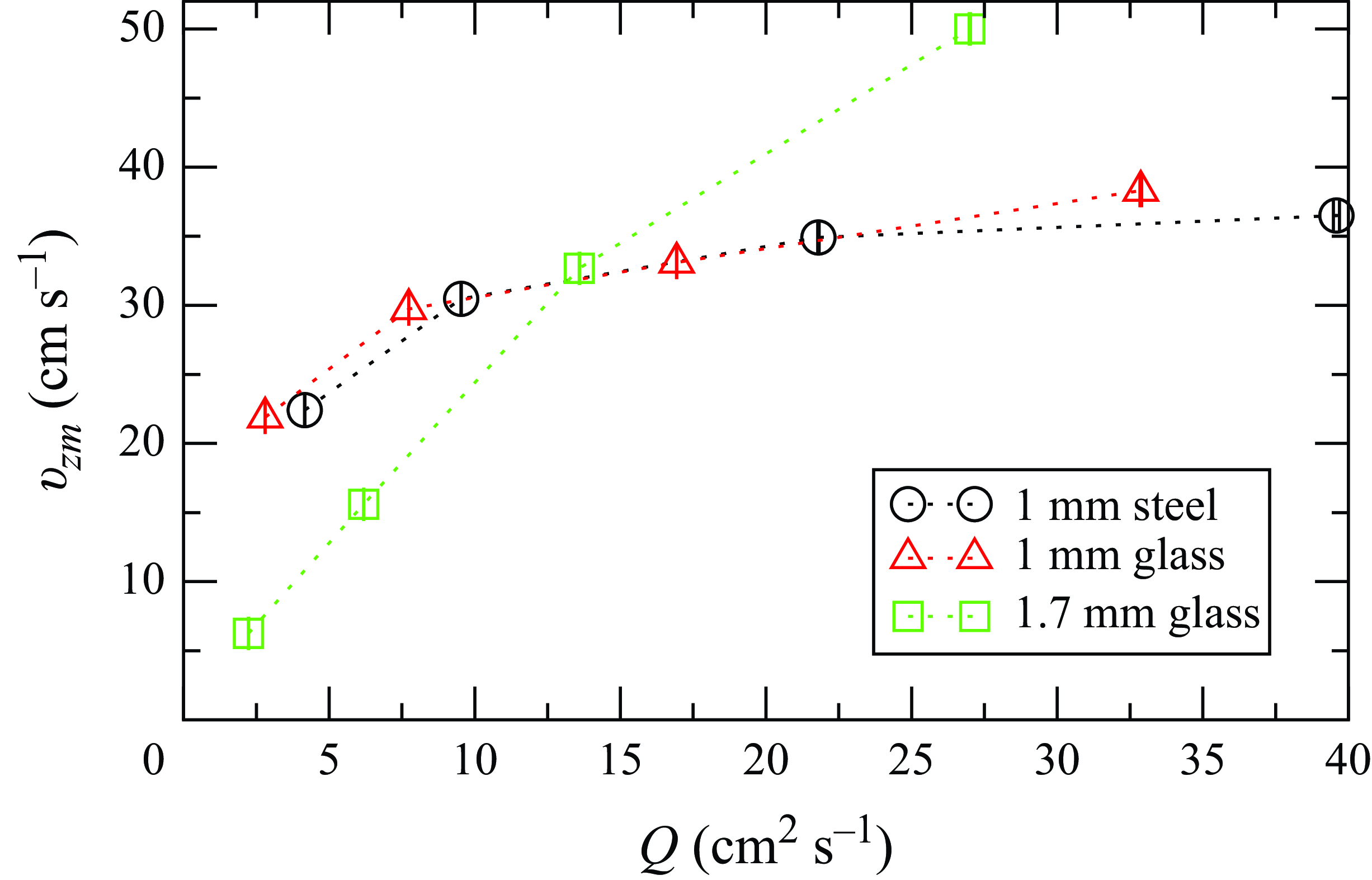
Variation of the maximum surface velocity ( $v_{zm}$
) with flow rate (
$v_{zm}$
) with flow rate ( $Q$
) for the different materials.
$Q$
) for the different materials.

Figure 9 shows the variation of $v_{zm}$
with volumetric flow rate per unit width (
$v_{zm}$
with volumetric flow rate per unit width ( $Q$
), referred to as ‘flow rate’ from here on for the sake of brevity, for the different materials. In general, as the flow rate is increased,
$Q$
), referred to as ‘flow rate’ from here on for the sake of brevity, for the different materials. In general, as the flow rate is increased, $v_{zm}$
also increases. However, as shown in figure 9, the rate of increase is much steeper for the larger glass beads (
$v_{zm}$
also increases. However, as shown in figure 9, the rate of increase is much steeper for the larger glass beads ( $v_{zm}$
increases by a factor of approximately
$v_{zm}$
increases by a factor of approximately $8.3$
for an 11-fold increase in flow rate), as opposed to the smaller particles (an increase in
$8.3$
for an 11-fold increase in flow rate), as opposed to the smaller particles (an increase in $v_{zm}$
by a factor of approximately
$v_{zm}$
by a factor of approximately $1.8$
for both stainless steel and glass beads, for a 9–11-fold increase in flow rate).
$1.8$
for both stainless steel and glass beads, for a 9–11-fold increase in flow rate).
From figure 9, we note that the rate of increase of $v_{zm}$
with flow rate (
$v_{zm}$
with flow rate ( $Q$
) is the same for the smaller particles irrespective of the type of material, while it is much higher for the larger particles. This highlights the important effect of particle size relative to particle density in slow granular surface flows and implies that inertial effects in the flow are small.
$Q$
) is the same for the smaller particles irrespective of the type of material, while it is much higher for the larger particles. This highlights the important effect of particle size relative to particle density in slow granular surface flows and implies that inertial effects in the flow are small.
Variation of the streamwise surface velocity ( $v_z$
) with transverse distance (
$v_z$
) with transverse distance ( $x$
) for different mass flow rates for 1.7 mm glass beads, when the distance from the pouring point to the front edge of the plate is (a)
$x$
) for different mass flow rates for 1.7 mm glass beads, when the distance from the pouring point to the front edge of the plate is (a) $L\;=\;14$
cm, (b)
$L\;=\;14$
cm, (b) $L\;=\;10$
cm and (c)
$L\;=\;10$
cm and (c) $L\;=\;8$
cm. The dashed lines correspond to the maximum surface velocities in each case. The origin of the
$L\;=\;8$
cm. The dashed lines correspond to the maximum surface velocities in each case. The origin of the $x$
axis is centred at the centre of the uni-directional flow region. The error bars represent standard error over three experiments.
$x$
axis is centred at the centre of the uni-directional flow region. The error bars represent standard error over three experiments.

Figure 10 shows the variation of streamwise velocity ( $v_z$
) along the transverse direction (
$v_z$
) along the transverse direction ( $x$
) for three different mass flow rates, for heaps formed using 1.7 mm glass beads, when the distance between the pouring point and the front edge of the plate (
$x$
) for three different mass flow rates, for heaps formed using 1.7 mm glass beads, when the distance between the pouring point and the front edge of the plate ( $L$
) is (a) 14 cm, (b) 10 cm and (c) 8 cm. As before, the dashed lines indicate the value of the maximum surface velocity (
$L$
) is (a) 14 cm, (b) 10 cm and (c) 8 cm. As before, the dashed lines indicate the value of the maximum surface velocity ( $v_{zm}$
) in each case. For all the cases, there is an increase in
$v_{zm}$
) in each case. For all the cases, there is an increase in $v_{zm}$
with mass flow rate (
$v_{zm}$
with mass flow rate ( $\dot {m}$
). The half-width of the central region (
$\dot {m}$
). The half-width of the central region ( $w_f$
), where the velocity profile is nearly flat, remains almost constant at approximately
$w_f$
), where the velocity profile is nearly flat, remains almost constant at approximately $40d$
with increase in the mass flow rates, even when the aspect ratio of the heap increases.
$40d$
with increase in the mass flow rates, even when the aspect ratio of the heap increases.
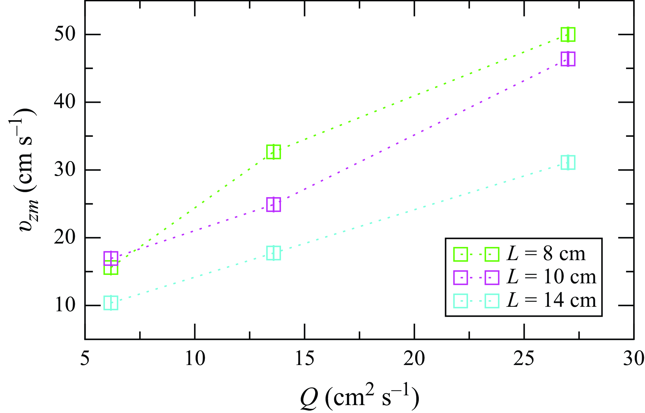
Variation of the maximum surface velocity ( $v_{zm}$
) with flow rate (
$v_{zm}$
) with flow rate ( $Q$
) for heaps of different aspect ratios.
$Q$
) for heaps of different aspect ratios.

Figure 11 summarises the variation of the maximum surface velocities with increasing flow rates for heaps of different aspect ratios, formed using the same material. As seen from figures 10 and 11, the flows become slower as the aspect ratio of the heap increases. From figure 11, it can be seen that $v_{zm}$
decreases by a factor of approximately
$v_{zm}$
decreases by a factor of approximately $1.63$
, as the aspect ratio of the heap increases by approximately
$1.63$
, as the aspect ratio of the heap increases by approximately $1.8$
times.
$1.8$
times.
3.2. Free surface angles
Variation of surface angle during steady surface flow ( $\beta _n$
) and angle of repose (
$\beta _n$
) and angle of repose ( $\beta _s$
) with volumetric flow rate (
$\beta _s$
) with volumetric flow rate ( $Q$
) for (a) 1 mm steel beads, (b) 1 mm glass beads and (c) 1.7 mm glass beads. The values of
$Q$
) for (a) 1 mm steel beads, (b) 1 mm glass beads and (c) 1.7 mm glass beads. The values of $\beta _n$
for heaps of different aspect ratios, formed using 1.7 mm glass beads, are shown in panel (c). The
$\beta _n$
for heaps of different aspect ratios, formed using 1.7 mm glass beads, are shown in panel (c). The $\beta$
-error bars denote the standard error for measurements over 200 frames for three independent measurements and the
$\beta$
-error bars denote the standard error for measurements over 200 frames for three independent measurements and the $Q$
-error bars denote standard errors for three independent measurements. The dashed lines are fits to the data.
$Q$
-error bars denote standard errors for three independent measurements. The dashed lines are fits to the data.

Figure 12 shows the variation of the surface angles during steady flow and for no flow for all the particles. The surface angle during steady flow is nearly constant at approximately $20.9^\circ$
for particles with mean diameter of 1 mm for both stainless steel and glass, even though the mass flow rate changes by a factor of 9–11 . The surface angle during steady flow remains constant at approximately
$20.9^\circ$
for particles with mean diameter of 1 mm for both stainless steel and glass, even though the mass flow rate changes by a factor of 9–11 . The surface angle during steady flow remains constant at approximately $20.7^\circ$
for the bigger glass particles over an 11-fold increase in mass flow rate. The invariance of
$20.7^\circ$
for the bigger glass particles over an 11-fold increase in mass flow rate. The invariance of $\beta _n$
with flow rates is also observed when the distance of the pouring point from the front edge of the plate increases. This is in remarkable contrast to quasi-two-dimensional wall bounded surface flows, where the wall friction aids in the increase of surface angles with increase in flow rates for a fixed width (Khakhar et al. Reference Khakhar, Orpe, Andresen and Ottino2001; Taberlet et al. Reference Taberlet, Richard, Valance, Losert, Pasini, Jenkins and Delannay2003) and hence, the difference between
$\beta _n$
with flow rates is also observed when the distance of the pouring point from the front edge of the plate increases. This is in remarkable contrast to quasi-two-dimensional wall bounded surface flows, where the wall friction aids in the increase of surface angles with increase in flow rates for a fixed width (Khakhar et al. Reference Khakhar, Orpe, Andresen and Ottino2001; Taberlet et al. Reference Taberlet, Richard, Valance, Losert, Pasini, Jenkins and Delannay2003) and hence, the difference between $\beta _n$
and
$\beta _n$
and $\beta _s$
also increases with increasing flow rates. The surface angle during steady flow corresponds to the equilibrium neutral angle (
$\beta _s$
also increases with increasing flow rates. The surface angle during steady flow corresponds to the equilibrium neutral angle ( $\beta _n)$
, since at steady state, there is no erosion or deposition from the heap ((1.1) and (1.2)). Such an independence of the neutral angles on mass flow rates in the absence of side wall friction has been reported previously also in experiments by Mandal & Khakhar (Reference Mandal and Khakhar2019) and in simulations by Ray & Khakhar (Reference Ray and Khakhar2021). These surface angles are close to the lowest angles at which stable flow is possible for flow of a
$\beta _n)$
, since at steady state, there is no erosion or deposition from the heap ((1.1) and (1.2)). Such an independence of the neutral angles on mass flow rates in the absence of side wall friction has been reported previously also in experiments by Mandal & Khakhar (Reference Mandal and Khakhar2019) and in simulations by Ray & Khakhar (Reference Ray and Khakhar2021). These surface angles are close to the lowest angles at which stable flow is possible for flow of a $\gt 30d$
thick layer of particles on a rough inclined plane (Silbert et al. Reference Silbert, Ertaş, Grest, Halsey, Levine and Plimpton2001).
$\gt 30d$
thick layer of particles on a rough inclined plane (Silbert et al. Reference Silbert, Ertaş, Grest, Halsey, Levine and Plimpton2001).
The angles of repose ( $\beta _s$
), surface angle in the limit of no flow, are also independent of the flow rates prior to the static condition, and are measured to be approximately
$\beta _s$
), surface angle in the limit of no flow, are also independent of the flow rates prior to the static condition, and are measured to be approximately $19.1^\circ$
for stainless steel beads,
$19.1^\circ$
for stainless steel beads, $19.8^\circ$
for glass beads of
$19.8^\circ$
for glass beads of $1\;\mathrm {mm}$
mean diameter and
$1\;\mathrm {mm}$
mean diameter and $19.0^\circ$
for glass beads of
$19.0^\circ$
for glass beads of $1.7\;\mathrm {mm}$
mean diameter. The differences between the steady-state surface angle (
$1.7\;\mathrm {mm}$
mean diameter. The differences between the steady-state surface angle ( $\beta _n$
) and the angle of repose (
$\beta _n$
) and the angle of repose ( $\beta _s$
) range from 1.2
$\beta _s$
) range from 1.2 $^{\circ }$
to 1.8
$^{\circ }$
to 1.8 $^{\circ }$
and show that in the absence of side wall friction, surface flow occurs with a very small driving force. This is in contrast to quasi-two-dimensional wall bounded surface flows, where the wall friction aids in the increase of surface angles with increase in flow rates (Khakhar et al. Reference Khakhar, Orpe, Andresen and Ottino2001; Taberlet et al. Reference Taberlet, Richard, Valance, Losert, Pasini, Jenkins and Delannay2003; Jop et al. Reference Jop, Forterre and Pouliquen2005) and hence, the difference between
$^{\circ }$
and show that in the absence of side wall friction, surface flow occurs with a very small driving force. This is in contrast to quasi-two-dimensional wall bounded surface flows, where the wall friction aids in the increase of surface angles with increase in flow rates (Khakhar et al. Reference Khakhar, Orpe, Andresen and Ottino2001; Taberlet et al. Reference Taberlet, Richard, Valance, Losert, Pasini, Jenkins and Delannay2003; Jop et al. Reference Jop, Forterre and Pouliquen2005) and hence, the difference between $\beta _n$
and
$\beta _n$
and $\beta _s$
also increases with increasing flow rates. To cite an example, in the study by Jop et al. (Reference Jop, Forterre and Pouliquen2005), when the distance between the side walls is fixed at 1 cm (19 particle diameters), the difference between
$\beta _s$
also increases with increasing flow rates. To cite an example, in the study by Jop et al. (Reference Jop, Forterre and Pouliquen2005), when the distance between the side walls is fixed at 1 cm (19 particle diameters), the difference between $\beta _n$
and
$\beta _n$
and $\beta _s$
increases by approximately
$\beta _s$
increases by approximately $7^\circ$
when the volumetric flow rate per unit width increases by approximately
$7^\circ$
when the volumetric flow rate per unit width increases by approximately $28\;\mathrm {cm^2s^-{^1}}$
. For heap flows confined in thin channels, Taberlet et al. (Reference Taberlet, Richard, Valance, Losert, Pasini, Jenkins and Delannay2003) showed that the tangent of the angle of inclination of the heap free surface increases linearly as mass flow rates are increased. Khakhar et al. (Reference Khakhar, Orpe, Andresen and Ottino2001) also reported that for surface flows over heaps in the presence of frictional side walls, the angle at the free surface of the heap increases with local flow rates and the rate of increase is higher for smaller particles.
$28\;\mathrm {cm^2s^-{^1}}$
. For heap flows confined in thin channels, Taberlet et al. (Reference Taberlet, Richard, Valance, Losert, Pasini, Jenkins and Delannay2003) showed that the tangent of the angle of inclination of the heap free surface increases linearly as mass flow rates are increased. Khakhar et al. (Reference Khakhar, Orpe, Andresen and Ottino2001) also reported that for surface flows over heaps in the presence of frictional side walls, the angle at the free surface of the heap increases with local flow rates and the rate of increase is higher for smaller particles.
3.3. Flowing layer thickness and volumetric flow rate
Variation of the flowing layer thickness ( $\delta$
) with flow rate (
$\delta$
) with flow rate ( $Q$
) for the different materials and heaps of different aspect ratios. The error bars on the experimental values represent the standard error for six measurements.
$Q$
) for the different materials and heaps of different aspect ratios. The error bars on the experimental values represent the standard error for six measurements.

Figure 13 shows the variation of the flowing layer thickness ( $\delta$
) with flow rate (
$\delta$
) with flow rate ( $Q$
) for all the beads used in the experiments. The experimentally measured values of
$Q$
) for all the beads used in the experiments. The experimentally measured values of $\delta$
increase as flow rate increases. The rate of increase of flowing layer thickness with flow rate for the large particles is approximately half of that for the small particles, The measured values of
$\delta$
increase as flow rate increases. The rate of increase of flowing layer thickness with flow rate for the large particles is approximately half of that for the small particles, The measured values of $\delta$
from the experiments range between 4 and 19 particle diameters, indicating that the flowing layers are quite shallow (
$\delta$
from the experiments range between 4 and 19 particle diameters, indicating that the flowing layers are quite shallow ( $\delta \;\lt \;20d$
). In general, the flows become thicker with increasing aspect ratios of the heap and the flowing layer depths increase by a factor of approximately
$\delta \;\lt \;20d$
). In general, the flows become thicker with increasing aspect ratios of the heap and the flowing layer depths increase by a factor of approximately $1.79$
for an increase in the aspect ratio of the heap by a factor of
$1.79$
for an increase in the aspect ratio of the heap by a factor of $1.8$
.
$1.8$
.
The volumetric flow rate per unit width in the central region, assuming a constant bulk density and a linear velocity profile with depth, as found in computations for a similar system (Ray & Khakhar Reference Ray and Khakhar2021), is
 \begin{equation} Q_{th}=\int _{0}^{\delta } v_{zm}\left (1-\frac {y}{\delta }\right ){\rm d}y=\frac {v_{zm}\delta }{2}. \end{equation}
In figure 14, we compare the values of flow rates ( $Q_{th}$
), obtained from (3.1) using the measured surface velocities (
$Q_{th}$
), obtained from (3.1) using the measured surface velocities ( $v_{zm}$
) and flowing layer thicknesses (
$v_{zm}$
) and flowing layer thicknesses ( $\delta$
), with the values of the measured flow rates (
$\delta$
), with the values of the measured flow rates ( $Q$
) (table 1). The dashed line in figure 14 represents a straight line with unit slope, and all the points from the experiments with different materials and sizes lie in close proximity to this line, indicating that the values of flow rates predicted from (3.1) are in excellent agreement with the flow rates measured directly from experiments. This also validates the assumption of a linear velocity profile in the flowing layer.
$Q$
) (table 1). The dashed line in figure 14 represents a straight line with unit slope, and all the points from the experiments with different materials and sizes lie in close proximity to this line, indicating that the values of flow rates predicted from (3.1) are in excellent agreement with the flow rates measured directly from experiments. This also validates the assumption of a linear velocity profile in the flowing layer.
Comparison between measured flow rates and flow rates estimated from (3.1) for the different materials used in the experiments and for heaps of different aspect ratios. The dashed line has a unit slope.

3.4. Scaling relations
In this section, we study the scaling between various quantities discussed in the preceding sections of the paper.
Scaled streamwise surface velocities ( $v_z/v_{zm}$
) versus the scaled transverse distance (
$v_z/v_{zm}$
) versus the scaled transverse distance ( $x/w_m$
), where
$x/w_m$
), where $w_m$
is the maximum width of the region of analysis.
$w_m$
is the maximum width of the region of analysis.

Figure 15 shows the streamwise velocities ( $v_z$
) scaled by the maximum surface velocities (
$v_z$
) scaled by the maximum surface velocities ( $v_{zm}$
) and the transverse distance by the maximum width of the region of analysis (
$v_{zm}$
) and the transverse distance by the maximum width of the region of analysis ( $w_m$
), chosen to ensure the best possible overlap of the scaled velocity profiles. The maximum width of the region of analysis (
$w_m$
), chosen to ensure the best possible overlap of the scaled velocity profiles. The maximum width of the region of analysis ( $w_m$
) differs slightly for each case. However, we choose this dimension as the scaling parameter, since the entire velocity profile, including points outside the central zone, is under consideration here. The graphs are also shifted along the
$w_m$
) differs slightly for each case. However, we choose this dimension as the scaling parameter, since the entire velocity profile, including points outside the central zone, is under consideration here. The graphs are also shifted along the $x$
axis to obtain a collapse of the scaled velocity profiles. The data for all the flow rates for both the materials collapse onto a single curve, as shown in figure 15. This indicates the velocity profiles for the different beads and flow rates are geometrically similar. Although not shown in the figure, the velocity profiles for the heaps with higher aspect ratios are also self-similar.
$x$
axis to obtain a collapse of the scaled velocity profiles. The data for all the flow rates for both the materials collapse onto a single curve, as shown in figure 15. This indicates the velocity profiles for the different beads and flow rates are geometrically similar. Although not shown in the figure, the velocity profiles for the heaps with higher aspect ratios are also self-similar.
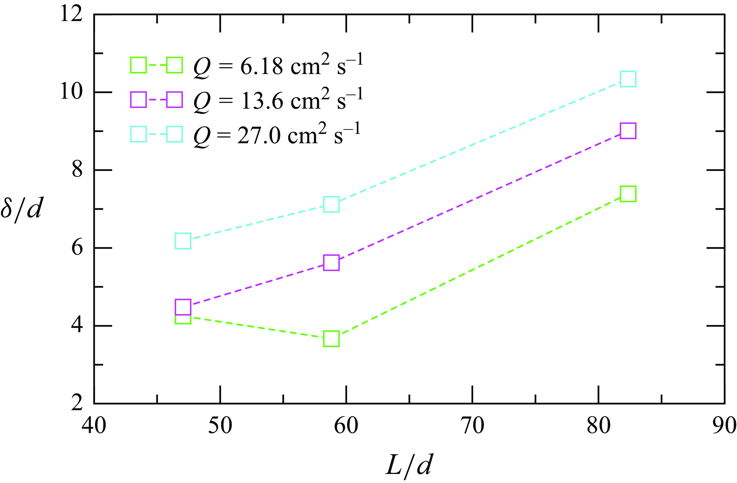
Variation of the scaled flowing layer thickness as a function of the scaled front to back length of the heap for the glass particles with 1.7 mm diameter.

Figure 16 shows that, at a fixed flow rate, the flowing layer thickness $\delta$
increases with increasing aspect ratio (i.e. increasing front to back length of the heap,
$\delta$
increases with increasing aspect ratio (i.e. increasing front to back length of the heap, $L$
). This shows that the flowing layer thickness is a function of the aspect ratio of the heap, and the length scale needs to be incorporated in the scaling analysis.
$L$
). This shows that the flowing layer thickness is a function of the aspect ratio of the heap, and the length scale needs to be incorporated in the scaling analysis.
Variation of the ratio of scaled flowing layer thickness ( $\bar {\delta }$
) to the scaled front to back length of the heap (
$\bar {\delta }$
) to the scaled front to back length of the heap ( $\bar {L}$
) as a function of scaled flow rate (
$\bar {L}$
) as a function of scaled flow rate ( $\bar {Q}$
). The black dashed line shows the best fit to the experimental data. The data points have been coloured according to their respective aspect ratios.
$\bar {Q}$
). The black dashed line shows the best fit to the experimental data. The data points have been coloured according to their respective aspect ratios.

The variation of the ratio of the scaled flowing layer thickness ( $\bar {\delta }=\delta /d$
) to the scaled front to back length of the heap (
$\bar {\delta }=\delta /d$
) to the scaled front to back length of the heap ( $\bar {L}=L/d$
) with the scaled flow rate (
$\bar {L}=L/d$
) with the scaled flow rate ( $\bar {Q}=Q/(gd^3)^{1/2}$
) is shown in figure 17. The data for all the materials collapse to a single straight line,
$\bar {Q}=Q/(gd^3)^{1/2}$
) is shown in figure 17. The data for all the materials collapse to a single straight line,
 \begin{equation} \frac {\bar {\delta }}{\bar {L}} = a\bar {Q} + b, \end{equation}
over a 10-fold increase in the scaled flow rate and an increase in the aspect ratio of the heap by a factor of 1.8, as shown in the figure. The slope and intercept of this line are $a=0.004$
and
$a=0.004$
and $b=0.071$
, respectively, and (3.2) fits the scaled experimental data with a correlation coefficient of
$b=0.071$
, respectively, and (3.2) fits the scaled experimental data with a correlation coefficient of $0.82$
. For a given aspect ratio of the heap, (3.2) indicates that
$0.82$
. For a given aspect ratio of the heap, (3.2) indicates that $\bar {\delta } \propto \bar {Q}$
, and there is a minimum layer thickness, below which, no surface flow is possible. Khakhar et al. (Reference Khakhar, Orpe, Andresen and Ottino2001) found
$\bar {\delta } \propto \bar {Q}$
, and there is a minimum layer thickness, below which, no surface flow is possible. Khakhar et al. (Reference Khakhar, Orpe, Andresen and Ottino2001) found $\bar {\delta }\propto \bar {Q}^{0.5}$
from experiments in quasi-2-D heaps and Fan et al. (Reference Fan, Umbanhowar, Ottino and Lueptow2013) found
$\bar {\delta }\propto \bar {Q}^{0.5}$
from experiments in quasi-2-D heaps and Fan et al. (Reference Fan, Umbanhowar, Ottino and Lueptow2013) found $\bar {\delta }\propto \bar {Q}^{0.22}$
based on simulations for flow of monodisperse particles in bounded heaps. For bounded conical heap flows (Isner et al. Reference Isner, Umbanhowar, Ottino and Lueptow2020a
), the power law exponent in the variation of scaled layer thickness to scaled flow rate is 0.46, whereas for frictional wedge-shaped heaps (Isner et al. Reference Isner, Umbanhowar, Ottino and Lueptow2020b
), the exponent is 2/7. The differences between these reported results and the present work are most likely due to side wall effects.
$\bar {\delta }\propto \bar {Q}^{0.22}$
based on simulations for flow of monodisperse particles in bounded heaps. For bounded conical heap flows (Isner et al. Reference Isner, Umbanhowar, Ottino and Lueptow2020a
), the power law exponent in the variation of scaled layer thickness to scaled flow rate is 0.46, whereas for frictional wedge-shaped heaps (Isner et al. Reference Isner, Umbanhowar, Ottino and Lueptow2020b
), the exponent is 2/7. The differences between these reported results and the present work are most likely due to side wall effects.
Variation of scaled maximum surface velocity ( $\bar {v}_{zm}$
) with scaled flow rate (
$\bar {v}_{zm}$
) with scaled flow rate ( $\bar {Q}$
). The dashed lines show the predictions of (3.3) against the experimental data points for the corresponding aspect ratios. The lines are of the same colour as the experimental data to which they correspnd.
$\bar {Q}$
). The dashed lines show the predictions of (3.3) against the experimental data points for the corresponding aspect ratios. The lines are of the same colour as the experimental data to which they correspnd.

Using the scaled form of (3.1) and substituting for $\bar {\delta }$
using (3.2), we get
$\bar {\delta }$
using (3.2), we get
 \begin{equation} \bar {v}_{zm}=\frac {2\bar {Q}}{(a\bar {Q}+b)\bar {L}}, \end{equation}
where the scaled maximum surface velocity is $\bar {v}_{zm}=v_{zm}/(gd)^{1/2}$
. Equation (3.3) implies that the variation of the scaled maximum surface velocities with scaled flow rates is influenced by the aspect ratio of the heap. This is evident from figure 18, where the dashed lines (predictions from (3.3)) match the experimental data with reasonable accuracy. The shear rate for this system can be estimated as
$\bar {v}_{zm}=v_{zm}/(gd)^{1/2}$
. Equation (3.3) implies that the variation of the scaled maximum surface velocities with scaled flow rates is influenced by the aspect ratio of the heap. This is evident from figure 18, where the dashed lines (predictions from (3.3)) match the experimental data with reasonable accuracy. The shear rate for this system can be estimated as $\dot {\gamma }={\rm d}v_z/{\rm d}y=v_{zm}/\delta$
. Then, using the linear scaling of
$\dot {\gamma }={\rm d}v_z/{\rm d}y=v_{zm}/\delta$
. Then, using the linear scaling of $\bar {\delta }$
with
$\bar {\delta }$
with $\bar {Q}$
for a specific aspect ratio of the heap, for scaled shear rates, we obtain
$\bar {Q}$
for a specific aspect ratio of the heap, for scaled shear rates, we obtain
 \begin{equation} \bar {\dot {\gamma }}=\frac {2\bar {Q}}{(a\bar {Q}+b)^2}, \end{equation}
where $\bar {\dot {\gamma }}=\dot {\gamma }/(g/d)^{1/2}$
is the scaled shear rate. Equation (3.4) implies a maximum in the scaled shear rate at
$\bar {\dot {\gamma }}=\dot {\gamma }/(g/d)^{1/2}$
is the scaled shear rate. Equation (3.4) implies a maximum in the scaled shear rate at $\bar {Q}=b/a$
; however, we could not verify this due to the scatter in the
$\bar {Q}=b/a$
; however, we could not verify this due to the scatter in the $\bar {\dot {\gamma }}$
data.
$\bar {\dot {\gamma }}$
data.
4. Conclusions
We report results of an experimental study of steady surface flow on heaps formed by pouring from a hopper with a rectangular slit outlet on a rough base comprising a shallow bed of the same particles. Steel balls and glass beads of two different sizes were used with different mass flow rates, obtained by varying the width of the slit exit. Surface velocities were measured using image analysis and the depth of the flow was obtained by immersing a soot-coated blade in the flow. Surface angles in the central region of the heap were measured by photography and image analysis, during flow and for the static heap. The surface flow was found to be uni-directional in the planar central region of the heap and became fully developed at short distances from the pouring point. The velocity in this region increases with flow rate and is nearly the same for the 1 mm steel and glass beads. The rate of increase of velocity with flow rate is higher for the large beads.
The neutral angles (surface angles during flow) are found to be nearly constant over a 10-fold increase in flow rate and are close to the minimum reported angles for flow on an inclined plane. The neutral angles exceed the static angles by 1.2 $^\circ$
–1.8
$^\circ$
–1.8 $^\circ$
, indicating a minimal driving force for the flow. The measured layer thicknesses range from 4 to 19 particle diameters and increase with flow rate. The data for 1 mm steel and glass beads are close and the rate of increase of thickness with flow rate is larger than that for the 1.7 mm glass beads. The negligible effect of a fold increase in density on the velocity and layer thickness indicates that inertia effects are negligible in the flow.
$^\circ$
, indicating a minimal driving force for the flow. The measured layer thicknesses range from 4 to 19 particle diameters and increase with flow rate. The data for 1 mm steel and glass beads are close and the rate of increase of thickness with flow rate is larger than that for the 1.7 mm glass beads. The negligible effect of a fold increase in density on the velocity and layer thickness indicates that inertia effects are negligible in the flow.
By adjusting the distance between the pouring point and the front edge of the rectangular plate, heaps of different aspect ratios were formed using the glass beads of 1.7 mm diameter. The flows were found to be slower and thicker for the bigger heaps, although the surface angles remained constant at approximately $20.7^\circ$
.
$20.7^\circ$
.
The scaled velocity profiles on the heap surface were found to collapse to a single curve and the scaled layer thickness ( $\bar {\delta }$
) was found to vary linearly with scaled flow rate (
$\bar {\delta }$
) was found to vary linearly with scaled flow rate ( $\bar {Q}$
), at a fixed aspect ratio of the heap, for all the particles and the different flow rates used. It was also observed that there exists a minimum layer thickness, below which no surface flow is possible for such systems, and the value of this critical layer thickness varies with heaps of varying aspect ratios. Using these relations and the assumption of a linear velocity variation with depth gave good predictions of the scaled surface velocity and the scaled shear rate, which exhibited a maximum.
$\bar {Q}$
), at a fixed aspect ratio of the heap, for all the particles and the different flow rates used. It was also observed that there exists a minimum layer thickness, below which no surface flow is possible for such systems, and the value of this critical layer thickness varies with heaps of varying aspect ratios. Using these relations and the assumption of a linear velocity variation with depth gave good predictions of the scaled surface velocity and the scaled shear rate, which exhibited a maximum.
The results presented in this work give a better understanding of surface granular flows on real three-dimensional heaps, in the absence of side wall friction. Such heaps are of importance in industrial and natural systems. The results obtained are qualitatively different from the behaviour reported for flow on heaps with frictional side walls.
Supplementary material
Supplementary material is available at https://doi.org/10.1017/jfm.2025.211
Acknowledgements
N.S.R. would like to acknowledge Dr Jeetram Yogi, for technical help during the experiments.
Funding
Partial financial support was received from the Science and Engineering Research Board, India, grant number SPR/2020/000301.
Declaration of interests
The authors report no conflict of interest.


 Open access