


1. Introduction
Feeding of oceanic microbes is essential for their biological fitness and ecological function (Solari et al. Reference Solari, Ganguly, Kessler, Michod and Goldstein2006; Guasto, Rusconi & Stocker Reference Guasto, Rusconi and Stocker2012; Elgeti, Winkler & Gompper Reference Elgeti, Winkler and Gompper2015; Gasol & Kirchman Reference Gasol and Kirchman2018; Shekhar et al. Reference Shekhar, Guo, Colin, Marshall, Kanso and Costello2023). The metabolic processes of microbes, from small bacteria to larger ciliates like the Stentor or Paramecium, hinge on the absorption of particles or molecules at their surface (Verni & Gualtieri Reference Verni and Gualtieri1997; Pettitt et al. Reference Pettitt, Orme, Blake and Leadbeater2002; Vopel et al. Reference Vopel, Reick, Arlt, Pöhn and Ott2002; Bialek Reference Bialek2012; Doelle Reference Doelle2014; Wan et al. Reference Wan, Hürlimann, Fenix, McGillivary, Makushok, Burns, Sheung and Marshall2020). These particles or molecules vary widely depending on the organism, and encompass dissolved oxygen and other gases, lightweight molecules, complex proteins, organic compounds, and small particles and bacteria. The typical random motion of these particles and bacteria is akin to a diffusive process at the scale of the microorganism (Berg & Purcell Reference Berg and Purcell1977; Magar, Goto & Pedley Reference Magar, Goto and Pedley2003; Magar & Pedley Reference Magar and Pedley2005; Michelin & Lauga Reference Michelin and Lauga2011; Berg Reference Berg2018). For simplicity, all cases will be referred to collectively as ‘nutrients’.
Ciliated microorganisms use surface cilia to generate flows in viscous fluids (Sládecek Reference Sládecek1981; Emlet Reference Emlet1990; Pettitt et al. Reference Pettitt, Orme, Blake and Leadbeater2002; Christensen-Dalsgaard & Fenchel Reference Christensen-Dalsgaard and Fenchel2003; Hartmann et al. Reference Hartmann, Özmutlu, Petermeier, Fried and Delgado2007; Kirkegaard & Goldstein Reference Kirkegaard and Goldstein2016). Ciliates either swim (Bullington Reference Bullington1930; Michelin & Lauga Reference Michelin and Lauga2010, Reference Michelin and Lauga2011; Guasto et al. Reference Guasto, Rusconi and Stocker2012; Andersen & Kiørboe Reference Andersen and Kiørboe2020) or attach to a surface and generate feeding currents (Sleigh & Barlow Reference Sleigh and Barlow1976; Vopel et al. Reference Vopel, Reick, Arlt, Pöhn and Ott2002; Zima-Kulisiewicz & Delgado Reference Zima-Kulisiewicz and Delgado2009; Pepper et al. Reference Pepper, Roper, Ryu, Matsudaira and Stone2010, Reference Pepper, Roper, Ryu, Matsumoto, Nagai and Stone2013; Andersen & Kiørboe Reference Andersen and Kiørboe2020; Wan et al. Reference Wan, Hürlimann, Fenix, McGillivary, Makushok, Burns, Sheung and Marshall2020). Whether motile or sessile, these ciliates perform work against the surrounding fluid, creating flow fields that affect the transport of nutrients and maintain a sufficient turnover rate of nutrients, unattainable by diffusion only (Solari et al. Reference Solari, Ganguly, Kessler, Michod and Goldstein2006). These nutrients can thus be modelled using a continuous concentration field subject to diffusion and advection by the microorganism's induced flows.
The coupling between diffusive and advective transport can be essential for microorganisms to achieve feeding rates that match their metabolic needs (Solari et al. Reference Solari, Ganguly, Kessler, Michod and Goldstein2006). The relative importance of advective transport is quantified by the Péclet number  $Pe = \tau _{diff}/\tau _{adv}$, defined as the ratio of diffusive $\tau _{diff}$ to advective $\tau _{adv}$ time scales. The diffusive time scale $\tau _{diff} = a^2/D$ is given by the typical size of the organism $a$ and the diffusivity $D$ of the nutrient of interest, while the advective time scale $\tau _{adv}= a/{\mathcal {U}}$ is governed by the flow speed ${\mathcal {U}}$ created by the microorganism.
To generate flows in a viscous fluid, a ciliated microorganism, through ciliary activity, must execute a series of irreversible surface deformations (Purcell Reference Purcell1977; Lauga & Powers Reference Lauga and Powers2009). We call such sequence of surface deformations a ‘stroke’. A stroke can induce a net force on the organism causing it to swim, or in the case of an attached organism, can require a reaction force, applied via a tether or a stalk, to resist swimming. Alternatively, the stroke itself could produce zero net force and be non-swimming. The question is, for a fixed rate of energy dissipation in the fluid, what are the optimal strokes that maximize nutrient flux at the organism's surface?
For a freely-moving organism, Michelin & Lauga (Reference Michelin and Lauga2011) showed that the ‘treadmill’ stroke, where on average all cilia exert tangential forces pointing from one end of the organism to the opposite end, is the only stroke that causes swimming. Importantly, Michelin & Lauga (Reference Michelin and Lauga2011) proposed that the treadmill stroke optimizes swimming and feeding at once for all  $Pe$ values. All other strokes were deemed suboptimal for feeding, even when considering unsteady strokes (Michelin & Lauga Reference Michelin and Lauga2013).
In this study, we evaluate, given a fixed amount of available energy, the effect of surface velocities on feeding rates in attached ciliated microorganisms and its comparison to swimming ciliated microorganisms. We consider a simplified spherical geometry, with the ciliated envelope modelled via a tangential slip velocity at the spherical surface (Blake Reference Blake1971). The Stokes equations are solved analytically using a linear decomposition of the ciliary stroke in terms of swimming and non-swimming modes (Blake Reference Blake1971; Magar et al. Reference Magar, Goto and Pedley2003; Michelin & Lauga Reference Michelin and Lauga2011), which we then optimize to maximize the organism's nutrient uptake for a given energetic cost.
Our results can be organized as follows. We first compare analytic solutions of the Stokes equations around the sessile and motile ciliated sphere. The difference in flow fields is fundamental and not reconcilable by a mere inertial transformation. We solve numerically the advection–diffusion equation around the sessile and motile sphere for a range of  $Pe$ values and for three distinct strokes: the treadmill mode, a symmetric dipolar mode, and a symmetric tripolar mode. Only the treadmill mode leads to swimming in the motile sphere case and requires a tethering force in the sessile case. By symmetry, higher-order modes are stationary, thus identical in the motile and sessile cases. We find that nutrient uptake depends non-trivially on $Pe$ values, and we successfully validate our numerical results by conducting an asymptotic analysis in the two limits of large and small $Pe$ for the sessile sphere, and comparing these asymptotic results to their counterparts in the motile case (Magar et al. Reference Magar, Goto and Pedley2003; Michelin & Lauga Reference Michelin and Lauga2011). We then turn to optimal feeding strokes in the sessile case, and seek, for a given amount of energy, the optimal stroke (possibly combining multiple simpler strokes) that maximizes nutrient uptake. We find consistent results through an open-loop search and an adjoint-based optimization method. We conclude by commenting on the implications of our findings to understanding biological diversity at the micron scale.
2. Mathematical formulation
2.1. Fluid flows around sessile and motile ciliates
The fluid velocity  $\boldsymbol {u}$ in a three-dimensional domain bounded internally by a spherical ciliate of radius $a$ (figure 1a) is governed by the incompressible Stokes equation (Kim & Karrila Reference Kim and Karrila2013)
 \begin{equation} {-}\boldsymbol{\nabla} p + \eta\,\nabla^2\boldsymbol{u} = 0,\quad \boldsymbol{\nabla}\boldsymbol{\cdot}\boldsymbol{u} = 0, \end{equation}
where  $p$ is the pressure field, and $\eta$ is the dynamic viscosity. To solve these equations, we consider the spherical coordinates $(r,\theta, \phi )$ and assume axisymmetric boundary conditions in $\phi$ at the spherical surface, with the axis of symmetry labelled by $z$, and the angle $\theta$ measured from the $z$-axis (figure 1a). For notational convenience, we introduce the unit vectors $\boldsymbol {e}_r,\boldsymbol {e}_\theta$, and unit vector $\boldsymbol {e}_z$ along the axis of symmetry, where $\boldsymbol {e}_z = \cos \theta \,\boldsymbol {e}_r - \sin \theta \,\boldsymbol {e}_\theta$ (figure 1a).
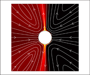
Modelling motile and sessile ciliates at zero Reynolds number. (a) Spherical envelope model with coordinates  $(r, \theta, \phi )$, where $\theta \in [0,{\rm \pi} ]$ and, due to axisymmetry, $\phi \in [0,2{\rm \pi} )$ is an ignorable coordinate. Ciliary motion is represented via a slip surface velocity. (b) First three modes of surface velocity all at the same energy value: treadmill (mode 1), dipolar (mode 2) and tripolar (mode 3), corresponding to $B_1\,V_1(\mu )$ ( $B_1=1$ for sessile and $B_1=\sqrt {3/2}$ for motile), $B_2\,V_2(\mu )$ and $B_3\,V_3(\mu )$, with $B_2=\sqrt {3}$, $B_3=\sqrt {6}$ for both sessile and motile. Dotted lines represent lines of symmetry of surface velocity. (c) Flow streamlines (white) and concentration fields (colour map) at $Pe=100$ (top row) and $1000$ (bottom row) for the same hydrodynamic power ${\mathcal {P}}=1$ and distinct surface motions. In the treadmill mode, the streamlines, concentration field and Sherwood number $Sh$ differ between the sessile and motile spheres, but are the same in the dipolar and tripolar surface modes.

Following Blake's envelope model (Blake Reference Blake1971), the cilia motion imposes a tangential slip velocity  $\boldsymbol {u}(r=a,\theta )= V\boldsymbol {e}_\theta$ at the surface of the spherical boundary. We introduce the nonlinear transformation $\mu = \cos \theta$ and expand $V =\sum _{n=1}^\infty B_n\,V_n(\mu )$ in terms of the basis functions $V_n(\mu )$ defined in terms of the Legendre polynomials $P_n(\mu )$ (see Appendix A). All modes result in surface velocities with $\phi$-axis rotational symmetry. For mode 1, $B_1 = 1$ and $B_n = 0$ for all $n\neq 1$, the ciliary surface motion is referred to as a ‘treadmill’ motion (figure 1b).
We distinguish between two cases: a sessile sphere, fixed in space, and a motile sphere moving at a swimming speed  $U$ in the $\boldsymbol {e}_z$ direction. The latter was considered in Blake (Reference Blake1971) and Michelin & Lauga (Reference Michelin and Lauga2010, Reference Michelin and Lauga2011). In the motile case, the coordinate system $(r,\theta )$ is attached to the sphere, and the equations of motion and boundary conditions are described in the body-fixed frame $(\boldsymbol {e}_r,\boldsymbol {e}_\theta )$. We get two sets of boundary conditions:
 \begin{equation} \left.\begin{array}{ll@{}}
\displaystyle {\rm Sessile} & \boldsymbol{u}|_{r
= a} = \sum_{n=1}^\infty B_n\,V_n(\mu)\,
\boldsymbol{e}_\theta, \quad \boldsymbol{u}|_{r\to\infty} =
\boldsymbol{0},\\ \displaystyle {\rm Motile} &
\boldsymbol{u} |_{r = a} = \sum_{n=1}^\infty
B_n\,V_n(\mu)\, \boldsymbol{e}_\theta, \quad
\boldsymbol{u}|_{r\to\infty} ={-}U\boldsymbol{e}_z.
\end{array}\right\} \end{equation}
\begin{equation} \left.\begin{array}{ll@{}}
\displaystyle {\rm Sessile} & \boldsymbol{u}|_{r
= a} = \sum_{n=1}^\infty B_n\,V_n(\mu)\,
\boldsymbol{e}_\theta, \quad \boldsymbol{u}|_{r\to\infty} =
\boldsymbol{0},\\ \displaystyle {\rm Motile} &
\boldsymbol{u} |_{r = a} = \sum_{n=1}^\infty
B_n\,V_n(\mu)\, \boldsymbol{e}_\theta, \quad
\boldsymbol{u}|_{r\to\infty} ={-}U\boldsymbol{e}_z.
\end{array}\right\} \end{equation}
Substituting (2.2) into the general solution of (2.1), we obtain analytical expressions for the fluid velocity field and pressure field for sessile and motile sphere (see table 1).
Comparison of Stokes flow around sessile and motile ciliate models. Mathematical expressions are given for the fluid velocity field, pressure field, hydrodynamic power and forces acting on the sphere, for both sessile and motile ciliated spheres, and for the swimming speed for a freely swimming ciliated sphere. All quantities are given in dimensional form in terms of the radial distance  $r$ and angular variable $\mu =\cos \theta$.

In the motile case, we need an additional equation to solve for the swimming speed  $U$. This equation comes from consideration of force balance. The hydrodynamic force acting on the sphere is given by $\boldsymbol {F}_h = \int \boldsymbol {\sigma }\boldsymbol {\cdot }\hat {\boldsymbol {n}}\,\textrm {d}S$, where $\boldsymbol {\sigma } = -p\boldsymbol {I} + \eta ( \boldsymbol {\nabla }\boldsymbol {u} + \boldsymbol{\nabla}\boldsymbol{u}^\textrm{T})$ is the stress tensor, and $\hat {\boldsymbol {n}}$ is the unit normal from the sphere pointing into the fluid. The total hydrodynamic force $\boldsymbol {F}_h =0$ should be zero, leading to $U=2B_1/3$.
In the sessile case, the hydrodynamic force is balanced by an external force  $\boldsymbol {F}_t$, provided by a tether or stalk, that fixes the sphere in space. From force balance, $\boldsymbol {F}_t = -\boldsymbol {F}_h = - 4{\rm \pi} \eta a B_1\boldsymbol {e}_z$.
It is instructive to examine the leading-order term in the fluid velocity  $(u_r,u_\theta )$ in the sessile and motile cases (table 1). In the sessile case, the far-field fluid velocity is of order $1/r$, similar to that of a force monopole (Stokeslet). In the motile case, the far-field fluid velocity is of order $1/r^3$, as in the case of a three-dimensional potential dipole. The fluid velocity fields corresponding to the sessile and motile cases are not related to each other by a mere inertial transformation.
In order to compare sessile and motile ciliates that exert the same hydrodynamic power  ${\mathcal {P}}$ on the surrounding fluid, we introduce a characteristic velocity scale ${\mathcal {U}}$ based on the total hydrodynamic power ${\mathcal {U}} = \sqrt {{\mathcal {P}}/(8{\rm \pi} a\eta )}$. To obtain non-dimensional forms of the equations and boundary conditions, we consider the spherical radius $a=1$ and ${\mathcal {T}} = 1/{\mathcal {U}}=1$ as the characteristic length and time scales of the problem. These considerations impose the following constraints on the velocity coefficients ${B}_n$ (table 1):
 \begin{equation} {\rm Sessile}\quad\sum_{n=1}^{\infty} \dfrac{2{B}^2_n}{n(n+1)}=1,\quad {\rm Motile}\quad \dfrac{2}{3}\,{B}_1^2 + \sum_{n=2}^{\infty} \dfrac{2{B}^2_n}{n(n+1)}=1. \end{equation}
Considering only the treadmill mode leads to  $B_1 = 1$ in the sessile case, and $B_1 =\sqrt {3/2}$ in the motile case, with all other coefficients identically zero ( $B_{n\neq 1}=0$). That is, for the same hydrodynamic power ${\mathcal {P}}$, the sessile sphere exhibits a slower surface velocity than the motile sphere ( $B_1=1$ versus $B_1 =\sqrt {3/2}$), which can be proved using the reciprocal theorem (Happel & Brenner Reference Happel and Brenner1965) (see Appendix A). Considering only the second mode, we get $B_2 = \sqrt {3}$ and $B_{n\neq 2}=0$ in both the sessile and motile spheres, and when only the third mode is considered, $B_3=\sqrt {6}$ and $B_{n\neq 3}=0$ (figure 1b). In the sessile case, when a surface motion consists of multiple modes simultaneously, the portion of energy assigned to each mode is denoted by $\beta _n^2$, such that $B_n = \beta _n\,\sqrt {2/(n(n+1))}$. For example, if the total energy budget ${\mathcal {P}}$ is equally distributed between the first two modes, then we have $\beta _1^2=0.5$, $\beta _2^2=0.5$, and $B_1 = \sqrt {0.5}$, $B_2 = \sqrt {1.5}$.
2.2. Advection–diffusion model of nutrient concentration
To determine the effect of the advective flows generated by the ciliated sphere on the nutrient concentration field around the sphere, we consider the advection–diffusion equation for the steady-state concentration  $C$ of nutrients subject to zero concentration at the spherical surface (Berg & Purcell Reference Berg and Purcell1977; Magar et al. Reference Magar, Goto and Pedley2003; Michelin & Lauga Reference Michelin and Lauga2011; Bialek Reference Bialek2012):
 \begin{equation} \boldsymbol{u}\boldsymbol{\cdot} \boldsymbol{\nabla} C = D\,\Delta C, \quad C(\mu) |_{r=a=1} = 0,\quad C(\mu)|_{r\rightarrow\infty}= C_\infty. \end{equation}
We normalize the concentration field by its far-field value  $C_\infty$ at large distances away from the sphere, and consider the transformation of variables $c = (C_\infty - C)/C_\infty$ (Magar et al. Reference Magar, Goto and Pedley2003; Michelin & Lauga Reference Michelin and Lauga2011). Writing the advection–diffusion equation and boundary conditions (2.4) in non-dimensional form in terms of the new variable $c(r,\mu )$ yields
 \begin{equation} {Pe}\, {\boldsymbol{u}}\boldsymbol{\cdot}\boldsymbol{\nabla} {c} = \Delta {c},\quad {c}(\mu)|_{r=a=1} = 1,\quad {c}(\mu) |_{r\rightarrow\infty} = 0, \end{equation}
where the Péclet number  $Pe= a\,{\mathcal {U}}/D$ quantifies the ratio of diffusive to advective time scales. When advection is dominant, the advective time is much smaller than the diffusive time, and $Pe \gg 1$; when diffusion is dominant, the advective time is much larger, and $Pe \ll 1$. At $Pe =1$, the two processes are in balance.
We substitute the analytical solutions of the flow field  $\boldsymbol {u}$ from table 1 into (2.5). We arrive at governing equations for the concentration field $c$, which we solve analytically in the asymptotic limit of small and large Péclet numbers (see Appendix B), and numerically using a spectral method (see Appendix C).
2.3. Sherwood number
To quantify the uptake of nutrients at the surface of the sphere, we introduce the Sherwood number. The nutrient uptake rate is equal to the area integral of the concentration flux over the spherical surface
 \begin{equation} I ={-}\oint \hat{\boldsymbol{n}}\boldsymbol{\cdot} (- D\,\boldsymbol{\nabla} C) \,\text{d}S, \end{equation}
where  $\textrm {d}S = 2 {\rm \pi}a^2 \sin \theta \,\textrm {d}\theta$ is the element of surface area of the sphere. The sign convention is such that the concentration flux is positive if the sphere takes up nutrients. In the case of pure diffusion, the steady-state concentration obtained by solving the diffusion equation is given by $C(r) = C_\infty (1 - a/r)$, and the steady-state inward current due to molecular diffusion is given by
 \begin{equation} I_{diffusion} = 4 {\rm \pi}a DC_\infty. \end{equation}
Accounting for both advective and diffusive transport, the Sherwood number  $Sh$ is equivalent to a dimensionless nutrient uptake, where $I$ is scaled by $I_{diffusion}$:
 \begin{equation} Sh = \dfrac{I}{I_{diffusion}} ={-}\frac{1}{4{\rm \pi} a D C_\infty}\oint \hat{\boldsymbol{n}} \boldsymbol{\cdot} (- D\,\boldsymbol{\nabla} C) \,\text{d} S ={-}\frac{1}{2}\int_{{-}1}^1 \boldsymbol{\nabla} c\boldsymbol{\cdot}\boldsymbol{e}_r|_{r=a=1} \,{\rm d}\mu. \end{equation}
3. Results
3.1. Comparison of feeding rates in sessile and motile ciliates
In figure 1(c), we show the streamlines (white) around the motile and sessile spheres with slip surface velocity corresponding to the treadmill mode (mode 1), dipolar mode (mode 2) and tripolar mode (mode 3). In all cases, the hydrodynamic power  ${\mathcal {P}}/(8{\rm \pi} \eta a) = 1$ is held constant. Modes 2 and 3 produce zero net force on the sphere, causing no net motion even in the motile case, thus the streamlines are the same. Mode 1, the treadmill mode, is the only mode that leads to motility. The associated streamlines are shown in body-fixed frame in the motile case and in inertial frame in the sessile case.
The steady-state concentration field (colour map) is obtained from numerically solving the advection–diffusion equation around the motile and sessile spheres at  $Pe = 100$ and $1000$. In the treadmill mode, the motile sphere swims into regions of higher concentration, which thins the diffusive boundary layer at its leading surface, leaving a trailing plume or ‘tail’ of nutrient depletion. Similar concentration fields are obtained for the sessile sphere, albeit with wider trailing plumes, because, although the sphere is fixed, the surface treadmill velocity generates feeding currents that bring nutrients towards the surface of the sphere. In the dipolar and tripolar modes, feeding currents bring fresh nutrients to the spherical surface from, respectively, two opposite and three nearly equiangular directions.
We evaluated  $Sh$ associated with each mode at both $Pe = 100$ and $Pe= 1000$. Clearly, larger $Pe$ leads to higher nutrient uptake. In the treadmill mode, evaluating $Sh$ for the motile and sessile spheres led, respectively, to $7.6$ and $6.7$ at $Pe =100$, and to $23.2$ and $20.8$ at $Pe =1000$. Indeed, at each $Pe$, the motile sphere with treadmill surface velocity produced the largest $Sh$, implying that for the same hydrodynamic power, motility maximized nutrient uptake. But the percentage difference in nutrient uptake between the motile and sessile sphere decreased with increasing $Pe$, from $13.4\,\%$ to $11.5\,\%$. For the swimming sphere, comparing the treadmill mode and dipolar mode (mode 2), we found $Sh = 7.6$ and $6.0$ at $Pe=100$, and $Sh = 23.2$ and $22.7$ at $Pe=1000$. That is, for the motile sphere, the difference in nutrient uptake between mode 1 and mode 2 also decreased with increasing $Pe$ from $26.7\,\%$ to $2.2\,\%$. Interestingly, for the sessile sphere, the nutrient uptake in mode 2 ( $Sh = 22.7$) exceeded that of mode 1 ( $Sh = 20.8$) at $Pe = 1000$, with a $9.1\,\%$ increase.
To probe the trends in  $Sh$ over a larger range of $Pe$ values, we computed, for the same hydrodynamic power, the steady-state concentration field for the sessile and motile spheres, and for modes 1, 2 and 3, for $Pe \in [0,1000]$. The increment in $Pe$ is dynamically adjusted from $\Delta {Pe} = 0.01$ for $Pe<1$ (denser grid) to $\Delta {Pe} = 100$ for ${Pe} > 100$ (sparser grid), with $173$ discrete points in total between $Pe = 0$ and $Pe = 1000$. In figure 2(a), we show the results for the sessile sphere. The solid lines in blue, purple and grey represent modes 1, 2 and 3, respectively. Mode 1 exhibits the best feeding performance (highest $Sh$) for $Pe \leq 284$. Mode 2 exceeds mode 1 after this critical $Pe$ value. At $Pe = 1000$, the $Sh$ of mode 2 is approximately $10\,\%$ higher than that of mode 1. Numerical results for the motile sphere are shown in figure 2(b). Mode 1 outperforms modes 2 and 3 for the entire range of $Pe$ values, but the difference between modes 1 and 2 seems to decrease, and the two modes seem to approach each other asymptotically at larger $Pe$.
$Pe$.
Sherwood number as a function of Péclet number: (a) sessile ciliate model and (b) motile ciliate model for the same hydrodynamic power  ${\mathcal {P}}=1$. Solid lines are numerical calculations for mode 1 (blue), mode 2 (purple) and mode 3 (grey). Dashed lines and scaling laws in the limits of large and small $Pe$ are obtained from asymptotic analysis for mode 1 (blue) and mode 2 (purple).

To further understand the asymptotic behaviour of  $Sh$ in the limit of large $Pe$, we performed an asymptotic analysis to obtain the scaling of $Sh$ with $Pe$ (see Appendix B). To complete this analysis, we considered the two limits of small ${Pe} \ll 1$ and large ${Pe} \gg 1$ for the sessile ciliated sphere. Our approach is similar to that used in Magar et al. (Reference Magar, Goto and Pedley2003) and Michelin & Lauga (Reference Michelin and Lauga2011) for the treadmill mode in the motile ciliated sphere. In table 2, we summarize the results of our asymptotic analysis for modes 1 and 2 of the sessile sphere. Note that the asymptotic analysis of mode 2 applies equally to the sessile and motile spheres. For comparison reasons, we also include in this table the asymptotic results of Magar et al. (Reference Magar, Goto and Pedley2003) and Michelin & Lauga (Reference Michelin and Lauga2011) for the swimming ciliated sphere. These asymptotic results are superimposed onto the numerical computations in the two insets in figures 2(a,b).
Asymptotic expression for  $Sh$ as a function of $Pe$ for sessile and swimming ciliated sphere model. The velocity coefficients associated with each mode are chosen satisfying the same constraint hydrodynamic power.

At small  $Pe$ ( $Pe \ll 1$), in the treadmill mode, $Sh$ scales with $Pe^2$ and $Pe^1$, respectively, for the sessile and motile spheres, and in the dipolar mode, $Sh$ scales with $Pe^2$. That is, at $Pe\ll 1$, the treadmill mode outperforms the dipolar mode in the motile case, and the motile sphere outperforms the sessile sphere in the treadmill mode.
At large  $Pe$ ( $Pe \gg 1$), in the treadmill mode, $Sh$ scales with $\sqrt {Pe}$ in both the sessile and motile ciliated spheres. That is, there is no distinction in the scaling of $Sh$ with $Pe$ between the motile and sessile spheres. Interestingly, we found that in the dipolar mode, $Sh$ also scales with $\sqrt {Pe}$, indicating no distinction between the treadmill and dipolar modes. The constant coefficients in the asymptotic scaling differ slightly: $Sh \approx 0.65\sqrt {Pe}$ for treadmill, sessile, $Sh \approx 0.72\sqrt {Pe}$ for treadmill, motile, and $Sh \approx 0.74\sqrt {Pe}$ for dipolar, both. Thus in the motile sphere, the treadmill and dipolar modes perform nearly similarly in the large $Pe$ limit, while in the sessile sphere, the dipolar mode outperforms the treadmill mode by a distinguishable difference (by approximately $10\,\%$).
3.2. Optimal feeding in sessile ciliates
We next focused on the sessile ciliated sphere and, keeping the total hydrodynamic power constant, we investigated numerically how  $Sh$ varies when multiple surface modes coexist.
In figure 3(a), we distributed the total hydrodynamic power into the first two modes only, assigning a fraction  $\beta _1^2$ to mode 1, and the remaining fraction $1-\beta _1^2$ to mode 2. We varied $\beta _1^2$ from 1 (all hydrodynamic power assigned to mode 1) to 0 (all hydrodynamic power assigned to mode 2) at fixed intervals $\Delta \beta _1^2 = 0.05$. We also varied $Pe$ from $0$ to $1000$ at $\Delta {Pe} = 0.1$. For each combination $({Pe},\beta _1^2)$, we computed the steady state concentration field and calculated the resulting $Sh$. We found that at small $Pe$,
$Pe$,  $Sh$ increased monotonically as $\beta _1^2$ varied from 0 to 1, indicating that mode 1 is optimal. At larger $Pe$, a new local maximum appeared at $\beta _1^2=0$ (mode 2). This change is evident when comparing figures 3(b,c), which illustrate $Sh$ as a function of $\beta _1^2$ at $Pe = 10$ and $Pe = 1000$, respectively. At $Pe = 10$, the maximal $Sh$ at $\beta _1^2=1$ is a global optimum. At $Pe = 1000$, two local optima in $Sh$ are obtained at $\beta _1^2=1$ and $\beta _1^2=0$, with $Sh|_{\beta _1^2=0}>Sh|_{\beta _1^2=1}$, indicating that mode 2 is a global optimum. Interestingly, when calculating the sensitivity $\partial Sh/\partial \beta _1^2$ of these maxima to variations in $\beta _1^2$, we found that the maximum at $\beta _1^2=0$ (mode 2) is more sensitive to variations in $\beta _1^2$, with $|\partial Sh/\partial \beta _1^2 |_{\beta _1^2 = 0}\gg | \partial Sh/\partial \beta _1^2 |_{\beta _1^2 = 1}$. That is, a small variation in $\beta _1^2$ leads to larger drop in $Sh$ at $\beta _1^2 =0$ (mode 2), while the same variation in $\beta _1^2$ leads to a small drop in $Sh$ at $\beta _1^2 = 1$ (mode 1). In figure 3(c), we show that a $10\,\%$ variation of $\beta _1^2$ leads to a $3\,\%$ drop from the optimal value at mode 1, and a $20\,\%$ drop from the optimal value at mode 2.
Sherwood number for hybrid surface motions. (a) Hybrid surface motions with two fundamental modes, treadmill and dipolar, and constraint hydrodynamic power  ${\mathcal {P}}/(8{\rm \pi} \eta a) = \beta _1^2 +\beta _2^2 = 1$, where $\beta _1^2$ represents the portion of the energy assigned to mode 1. Plot of $Sh$ versus $Pe$ and $\beta _1^2$ as $\beta _1^2$ varies from $0$ to $1$. Close-ups of $Sh$ versus $\beta _1^2$ at (b) $Pe =10$ and (c) $Pe =1000$ (left) and partial derivative of $Sh$ with respect to $\beta _1^2$ (right). (d) Hybrid surface motions with three fundamental modes, treadmill, dipolar and tripolar, and constraint hydrodynamic power ${\mathcal {P}}/(8{\rm \pi} \eta a) = \beta _1^2 +\beta _2^2 + \beta _3^2= 1$, where $\beta _1^2$ and $\beta _2^2$ represent, respectively, the portions of the energy assigned to the treadmill and dipolar modes. Colour map shows variation in $Sh$ as we vary the energy portions $\beta _1^2$ and $\beta _2^2$ in the first two modes. Grey regions marked by red dashed lines correspond to $Sh$ within 10 % of corresponding maximal $Sh$.
$Sh$.

We next considered the case when the total hydrodynamic power  ${\mathcal {P}}$ is distributed over the first three modes, with a fraction $\beta _1^2$ assigned to mode 1, a fraction $\beta _2^2$ assigned to mode 2, and the remaining fraction $(1 - \beta _1^2 - \beta _2^2)$ assigned to mode 3. We considered five values of $Pe =10, 100, 200, 500, 1000$. For each $Pe$ value, we varied $\beta _1^2$ and $\beta _2^2$ from 0 to 1 at $\Delta \beta ^2_{(\cdot )} = 0.1$, computed the steady-state concentration field at each grid point, and evaluated the corresponding $Sh$. Results are shown in figure 3(d). A similar trend appears: at small $Pe$, feeding is optimal when all the energy is assigned to mode 1 ( $\beta _1^2 = 1$, $\beta _2^2 = 0$), but as $Pe$ increases, a new local optimum appears at mode 2 ( $\beta _1^2 = 0$, $\beta _2^2 = 1$). To test the sensitivity of these optima to variations in surface motion, we highlighted in light grey regions in the $(\beta _1^2,\beta _2^2)$ space that correspond to a 10 % drop in $Sh$ from the corresponding optimal value. Although at high $Pe$, mode 2 reaches higher values of $Sh$, it is more sensitive to variations in surface motion. The local optimum at mode 1 is more robust to such perturbations.
The optima in figure 3 are identified in an open-loop search over the parameter spaces  $(\beta _1^2, {Pe})$ and $(\beta _1^2,\beta _2^2,{Pe})$. Such an open-loop search becomes unfeasible when considering higher-order surface modes. A closed-loop optimization algorithm that seeks surface velocities that optimize $Sh$ is needed. Here, we adapted the adjoint optimization method with gradient ascent algorithm used in Michelin & Lauga (Reference Michelin and Lauga2011) (see Appendix D).
In figure 4, we considered initial surface velocities with 10 modes, satisfying the constraint on the total hydrodynamic power  $\sum _{n=1}^N \beta _n^2 = 1$. We used the closed-loop optimization algorithm to identify optimal surface velocities that maximize $Sh$. In figure 4(a), we show the optimization results at $Pe = 10$ and two distinct initial conditions (grey line). The optimization algorithm converges to an optimal solution (black line) that is close to mode 1 (superimposed in blue). The energy distribution among all modes as a function of iteration steps shows that while the initial energy was distributed among multiple modes, in the converged solution, energy is assigned mostly to mode 1. Indeed, comparing $Sh$ (black marker $\ast$) to $Sh$ of mode 1 (blue line) shows that the optimal $Sh$ converges to that of mode 1. Flow streamlines and concentration fields at these optima are shown in the bottom row of figure 4(a).
Numerical optimization of surface motions that maximize feeding rates in sessile ciliates. (a) Optimization results at  $Pe = 10$ for two different initial guesses. (b) Optimization results at $Pe = 1000$ for the same two different initial guesses. The top row shows initial surface velocity (grey), optimal surface motion (black), and mode 1 (blue). The second row shows the energy distribution among ten different velocity modes at each iteration of the numerical optimization process. The third row shows $Sh$ (black) at each iteration, $Sh$ for only mode 1 ( $Sh_{mode 1}$, blue), and the difference in $Sh$ ( $Sh_{mode 1}-Sh$, grey). The last row shows fluid and concentration fields under optimal surface conditions. In (b), at $Pe =1000$, the numerical optimization algorithm converges to one of two distinct solutions, depending on initial conditions that are close to either mode 1 (blue) or mode 2 (purple).

In figure 4(b), we show the optimization results at  $Pe = 1000$ and the same two initial conditions (grey line) considered in figure 4(a). Here, unlike in figure 4(a), the optimization algorithm converges to two different optimal solutions depending on initial conditions: one optimal (black line) is close to mode 1 (superimposed in blue), and the other optimal is close to mode 2 (superimposed in purple), as reflected in the energy distribution (second row) and in $Sh$ values (third row). Flow streamlines and concentration fields at these two distinct optima are shown in the bottom row of figure 4(b). The second optimal, the one corresponding to mode 2, exhibits the higher $Sh$ value. These results are consistent with the open-loop analysis presented in figures 2 and 3.
4. Conclusion
This work outlines several novel contributions. (1) We extended the envelope model to a fixed ciliated sphere. (2) We analysed the feeding rates around fixed and freely swimming spheres, subject to steady-state surface velocities, and computed the Sherwood number  $Sh$ numerically in a range of moderate Péclet numbers $Pe$. (3) We performed asymptotic analysis for $Sh$ as a function of $Pe$ in the two extreme (small and large) $Pe$ limits, and for the two first modes of surface velocities. (4) We computed optimal surface velocities that maximize feeding rates using an adjoint feedback optimization method.
For motile ciliates, we found that assigning all energy into a treadmill surface velocity that induces swimming is an optimal strategy for maximizing feeding rate, but only in a finite  $Pe$ range. This is in contrast to the findings in Michelin & Lauga (Reference Michelin and Lauga2011) that claimed optimality of the treadmill mode for all $Pe$. In the limit of large $Pe$, we found no distinction in nutrient uptake between the treadmill mode and the symmetric dipolar mode that applies zero net force on the ciliated body, inducing no swimming motion.
For sessile ciliates, we found that the treadmill mode achieves optimal feeding rate at relatively low  $Pe$ values below a critical value $Pe_{cr} \approx 280$, while the dipolar mode becomes optimal for $Pe$ exceeding this threshold. Our asymptotic analysis supports that in the large $Pe$ limit, the dipolar surface mode outperforms other modes in terms of feeding rate. However, our sensitivity analysis shows that although at large $Pe$ the treadmill mode leads to lower $Sh$, it is more robust to perturbations in the surface velocity. The dipolar mode leads to higher $Sh$, but it is significantly more sensitive to perturbations, with feeding efficiency dropping rapidly even with small perturbations in surface motion.
The reader may wonder how the optimal solutions discussed here apply to unsteady, time-dependent ciliary strokes. In a follow-up study to Michelin & Lauga (Reference Michelin and Lauga2011), which focused solely on motile ciliates, the authors numerically explored unsteady strokes for maximizing feeding at a fixed energy budget, and found that the optimal steady swimmer was always the overall optimal feeder (Michelin & Lauga Reference Michelin and Lauga2013). Similarly, in a preliminary analysis of unsteady surface motions, we found that in both motile and sessile ciliates, the optimal steady-state solutions presented in this work set an upper bound for what is achievable in the unsteady case. These unsteady motions will be explored in future work.
Our findings challenge previous assumptions that motility inherently improves feeding rate in ciliates (Michelin & Lauga Reference Michelin and Lauga2011; Andersen & Kiørboe Reference Andersen and Kiørboe2020). We demonstrate that the optimal cilia-driven surface velocity for maximizing feeding rate varies significantly depending on  $Pe$, with distinct advantages observed for both motile and sessile ciliates under different $Pe$. This study enriches the understanding of the complexity of feeding strategies in ciliated microorganisms, and highlights the importance of considering various environmental conditions when evaluating the ecological roles and evolutionary adaptations of these microbes.
Funding
This work was supported by by the National Science Foundation grants RAISE IOS-2034043 (E.K.), CBET-210020 (E.K.) and NSF 2100705 (J.H.C.), and the Office of Naval Research grants N00014-22-1-2655 (E.K.), N00014-19-1-2035 (E.K.) and N00014-23-1-2754 (J.H.C).
Declaration of interests
The authors report no conflict of interest.
Author contributions
E.K. designed and supervised research. J.L. conducted research, with technical input from Y.M. J.L., J.H.C. and E.K. analysed results. J.L. and E.K. wrote the manuscript, and all authors reviewed and approved the submission.
Appendix A. General solution of the Stokes equations in spherical coordinates
A.1. Stokes equations
For solving fluid velocity  $\boldsymbol {u}$ at zero $Re$ limit, the incompressible Stokes equation, we consider following approach. Due to the continuity property of the fluid, the velocity vector $\boldsymbol {u}$ can be expressed in terms of a vector potential $\varPsi$ as $\boldsymbol {u}=\boldsymbol {\nabla }\times \varPsi$ (Batchelor Reference Batchelor2000). Taking the curl of the Stokes equation in (2.1), substituting $\boldsymbol {u}=\boldsymbol {\nabla }\times \varPsi$ into the resulting equation and using the incompressibility condition, we get the classic result that the vector potential $\varPsi$ is governed by the bi-Laplacian $\nabla ^2\nabla ^2\varPsi =0$ (Happel & Brenner Reference Happel and Brenner1965).
To solve for the fluid velocity in the fluid domain bounded internally by a spherical boundary of radius  $a$, it is convenient to introduce the spherical coordinates $(r,\theta,\phi )$ and associated unit vectors $\boldsymbol {e}_r,\boldsymbol {e}_\theta,\boldsymbol {e}_\phi$ (see figure 1a). We express the fluid velocity in component form $\boldsymbol {u}\equiv (u_r,u_\theta,u_\phi )$. Here, we are interested only in axisymmetric flows, for which $u_\phi =0$ is identically zero, and the components of the vector potential $\varPsi$ can be expressed in terms of an axisymmetric streamfunction $\psi$ (see e.g. Batchelor Reference Batchelor2000):
 \begin{equation} \varPsi=\left(0,0,\frac{\psi}{r\sin\theta}\right)^{{\rm T}}. \end{equation}
The non-trivial components  $(u_r,u_\theta )$ of the fluid velocity are related to $\psi (r,\theta )$ as follows:
 \begin{equation} u_{r} =\frac{1}{r^{2}\sin\theta}\,\frac{\partial\psi}{\partial\theta},\quad u_{\theta} ={-}\frac{1}{r\sin\theta}\,\frac{\partial\psi}{\partial r}. \end{equation}
The streamfunction  $\psi$ is governed by the biharmonic equation $E^2E^2(\psi )=0$ given in terms of the linear operator $E^2$:
 \begin{equation} E^{2}=\frac{\partial^{2}}{\partial r^{2}}+\frac{\sin\theta}{r^{2}}\,\frac{\partial}{\partial\theta} \left(\frac{1}{\sin\theta}\,\frac{\partial}{\partial\theta}\right). \end{equation}
This biharmonic equation  $E^2E^2(\psi )=0$ can be solved analytically for arbitrary boundary conditions in terms of $r$ and the coordinate $\mu$ obtained via the nonlinear transformation of coordinates $\mu = \cos \theta$. Explicitly, an expression for $\psi (r,\mu )$ can be found in Happel & Brenner (Reference Happel and Brenner1965):
 \begin{equation} \psi(r,\mu)=\sum_{n=2}^{\infty}(a_{n}r^{n}+b_{n}r^{{-}n+1}+c_{n}r^{n+2}+d_{n}r^{{-}n+3})\,F_{n}(\mu). \end{equation}
Here,  $F_n(\mu )= -\int P_{n-1}(\mu )\,\textrm {d}\mu$ are solution functions related to the Legendre polynomials of the first kind $P_{n}(\mu )$, satisfying the equation $(1-\mu ^{2})({\textrm {d}^{2}F_n}/{\textrm {d}\mu ^{2}})+n(n-1)F_n = 0$, and $a_{n}$, $b_{n}$, $c_n$ and $d_n$ are unknown coefficients.
By substituting (A4) into (A2), we obtain the velocity components  $(u_r,u_\theta )$:
 \begin{align} \left.\begin{array}{c@{}}
\displaystyle u_{r}(r,\mu) =\left(\alpha_0 +
\alpha_{13}\,\dfrac{1}{r^3}+\alpha_{11}\,\dfrac{1}{r}\right)P_{1}(\mu)
+ \sum_{n=2}^\infty \left(\alpha_{n+2}\,\dfrac{1}{r^{n+2}}
+ \alpha_{n}\,\dfrac{1}{r^{n}}\right)P_{n}(\mu),\\
\displaystyle u_{\theta}(r,\mu) = \left( -\alpha_{0} +
\alpha_{13}\,\dfrac{1}{2r^{3}} -
\alpha_{11}\,\dfrac{1}{2r}\right)V_{1}(\mu) +
\sum_{n=2}^\infty
\dfrac{1}{2}\left(\alpha_{n+2}\,\dfrac{n}{r^{n+2}} +
\alpha_{n}\,\dfrac{n-2}{r^{n}}\right)V_{n}(\mu),
\end{array}\right\} \end{align}
\begin{align} \left.\begin{array}{c@{}}
\displaystyle u_{r}(r,\mu) =\left(\alpha_0 +
\alpha_{13}\,\dfrac{1}{r^3}+\alpha_{11}\,\dfrac{1}{r}\right)P_{1}(\mu)
+ \sum_{n=2}^\infty \left(\alpha_{n+2}\,\dfrac{1}{r^{n+2}}
+ \alpha_{n}\,\dfrac{1}{r^{n}}\right)P_{n}(\mu),\\
\displaystyle u_{\theta}(r,\mu) = \left( -\alpha_{0} +
\alpha_{13}\,\dfrac{1}{2r^{3}} -
\alpha_{11}\,\dfrac{1}{2r}\right)V_{1}(\mu) +
\sum_{n=2}^\infty
\dfrac{1}{2}\left(\alpha_{n+2}\,\dfrac{n}{r^{n+2}} +
\alpha_{n}\,\dfrac{n-2}{r^{n}}\right)V_{n}(\mu),
\end{array}\right\} \end{align}
where  $\alpha _0, \alpha _{11}, \ldots, \alpha _n$ are unknown coefficients, related to $a_n, b_n, c_n, d_n$ in (A4), to be determined from boundary conditions. The basis functions $V_{n}(\mu )$ are defined as
 \begin{equation} V_{n}(\mu) ={-} \frac{2}{\sqrt{1-\mu^2}}\int P_{n}(\mu)\,{\rm d}\mu=\frac{2}{n(n+1)}\,\sqrt{1-\mu^2}\,P'_{n}(\mu), \end{equation}
where  $P_n'(\mu ) = {\textrm {d}P_n(\mu )}/{\textrm {d}\mu }$. Both the Legendre polynomials $P_n(\mu )$ and basis functions $V_n(\mu )$ satisfy the orthogonality conditions
 \begin{equation} \left.\begin{array}{c@{}}
\displaystyle
\int_{{-}1}^{{+}1}P_{n}(\mu)\,P_{m}(\mu)\,{\rm d}\mu
=\dfrac{2}{2n+1}\,\delta_{nm},\\ \displaystyle
\int_{{-}1}^{{+}1}V_{n}(\mu)\,V_{m}(\mu)\,{\rm d}\mu =
\dfrac{8}{n(n+1)(2n+1)}\,\delta_{mn}. \end{array}\right\}
\end{equation}
\begin{equation} \left.\begin{array}{c@{}}
\displaystyle
\int_{{-}1}^{{+}1}P_{n}(\mu)\,P_{m}(\mu)\,{\rm d}\mu
=\dfrac{2}{2n+1}\,\delta_{nm},\\ \displaystyle
\int_{{-}1}^{{+}1}V_{n}(\mu)\,V_{m}(\mu)\,{\rm d}\mu =
\dfrac{8}{n(n+1)(2n+1)}\,\delta_{mn}. \end{array}\right\}
\end{equation}
A.2. Analytical expressions of the pressure field
The pressure is obtained by substituting (A5) into the Stokes equation (2.1) and integrating, yielding the pressure field  $p(r,\mu )$ as
 \begin{equation} p = p_{\infty} + \eta \sum_{n=1}^{\infty}\frac{4n-2}{n+1}\,\frac{\alpha_n}{r^{n+1}}\,P_{n}(\mu). \end{equation}
A.3. Analytical expressions of the stress field
The fluid stress tensor  $\boldsymbol {\sigma }$ is given by $\boldsymbol {\sigma } = -p\boldsymbol {I} + \eta ( \boldsymbol {\nabla }\boldsymbol {u} + \boldsymbol {\nabla}\boldsymbol {u}^\textrm {T})$. For the axisymmetric flows considered here, $\boldsymbol {\sigma }$ admits three non-trivial stress components:
 \begin{equation} \left.\begin{array}{c@{}} \displaystyle \sigma_{rr} ={-}p+2\eta\,\dfrac{\partial u_{r}}{\partial r},\quad \sigma_{r\theta} = \eta\left(\dfrac{1}{r}\,\dfrac{\partial u_r}{\partial\theta}+r\,\dfrac{\partial}{\partial r}\left(\dfrac{u_{\theta}}{r}\right)\right),\\ \displaystyle \sigma_{\theta\theta} ={-}p +2\eta \left(\dfrac{1}{r}\,\dfrac{\partial u_\theta}{\partial\theta}+\dfrac{u_r}{r}\right). \end{array}\right\} \end{equation}
Explicit expressions for the stress components are obtained by substituting (A5) and (A8) into (A9).
A.4. Hydrodynamic force acting on the sphere
The hydrodynamic force exerted by the fluid on the sphere can be calculated by integrating the stress tensor  $\boldsymbol {\sigma }$ over the surface $S$ of the sphere. Due to axisymmetry, only the force in the direction of the axis of axisymmetry, taken to be the $z$-axis, is non-zero:
 \begin{equation} \boldsymbol{F} = \int_S \boldsymbol{\sigma}\boldsymbol{\cdot} \hat{\boldsymbol{n}}\,\textrm{d}S ={-}4{\rm \pi}\eta \alpha_{11}\boldsymbol{e}_z. \end{equation}
A.5. Viscous dissipation energy
The energy dissipation rate is defined as the volume integral over the entire fluid domain  $V$ of the inner product of the velocity strain rate tensor $\boldsymbol {e} = \frac {1}{2}(\boldsymbol {\nabla }\boldsymbol {u} + \boldsymbol {\nabla }\boldsymbol {u}^\textrm {T})$ and stress tensor $\boldsymbol {\sigma }$, which, given proper decay at infinity, can be expressed as an integral over the surface of the sphere by applying the divergence theorem (see e.g. Kim & Karrila Reference Kim and Karrila2013),
 \begin{equation} {\mathcal{P}} = \int_V \boldsymbol{e}:\boldsymbol{\sigma} \,\textrm{d}V ={-} \int_{S} \boldsymbol{u}\boldsymbol{\cdot}(\boldsymbol{\sigma}\boldsymbol{\cdot}\hat{\boldsymbol{n}}) \,\textrm{d}S. \end{equation}
A.6. Energy dissipation and the reciprocal theorem
Let  $\boldsymbol {u}_1$ and $\boldsymbol {\sigma }_1$ be the fluid velocity and stress field at the surface of the sessile ciliate, and let $\boldsymbol {u}_m = U\boldsymbol {e}_z + \boldsymbol {u}_{1}$ and $\boldsymbol {\sigma }_m$ be those of the motile ciliate; here, $U\boldsymbol {e}_z$ represents the rigid translation of the ciliate and $\boldsymbol {u}_{1}$ the ciliary treadmill motion, assuming that both motile and sessile ciliates exhibit the same $\boldsymbol {u}_{1}$. The total energy dissipation rates ${\mathcal {P}}_s$ and ${\mathcal {P}}_m$ of the sessile and motile ciliates, respectively, are given by
 \begin{equation} {\mathcal{P}}_s ={-} \oint \boldsymbol{u}_{1}\boldsymbol{\cdot}\boldsymbol{\sigma}_1\boldsymbol{\cdot} \hat{\boldsymbol{n}}\,{\rm d}S, \quad {\mathcal{P}}_m ={-} \oint \boldsymbol{u}_m\boldsymbol{\cdot}\boldsymbol{\sigma}_m\boldsymbol{\cdot} \hat{\boldsymbol{n}}\,{\rm d}S ={-} \oint \boldsymbol{u}_{1}\boldsymbol{\cdot}\boldsymbol{\sigma}_m\boldsymbol{\cdot} \hat{\boldsymbol{n}}\,{\rm d}S, \end{equation}
where, to obtain  ${\mathcal {P}}_m$, we used the fact that $\oint \boldsymbol {e}_z\boldsymbol {\cdot }\boldsymbol {\sigma }_m\boldsymbol {\cdot } \hat {\boldsymbol {n}}\,\textrm {d}S =0$ because the motile ciliate is force-fee in the $\boldsymbol {e}_z$ direction.
Now apply the reciprocal theorem (Happel & Brenner Reference Happel and Brenner1965) to the two auxiliary problems  $(\boldsymbol {u}_{1}, \boldsymbol {\sigma }_{1})$ and $(\boldsymbol {u}_{m}: \boldsymbol {\sigma }_{m})$,
 \begin{equation} \oint \boldsymbol{u}_1\boldsymbol{\cdot}\boldsymbol{\sigma}_m\boldsymbol{\cdot} \hat{\boldsymbol{n}}\,{\rm d}S = \oint \boldsymbol{u}_m\boldsymbol{\cdot}\boldsymbol{\sigma}_1\boldsymbol{\cdot} \hat{\boldsymbol{n}}\,{\rm d}S. \end{equation}
The left-hand side is equal to  ${\mathcal {P}}_m$. The right-hand side, recalling that $\boldsymbol {u}_m = U\boldsymbol {e}_z + \boldsymbol {u}_{1}$, is equal to ${\mathcal {P}}_s - U\oint \boldsymbol {e}_z \boldsymbol {\cdot } \boldsymbol {\sigma }_1\boldsymbol {\cdot } \hat {\boldsymbol {n}}\,\textrm {d}S$, that is,
 \begin{equation} {\mathcal{P}}_m = {\mathcal{P}}_s - U\oint \boldsymbol{e}_z \boldsymbol{\cdot} \boldsymbol{\sigma}_1\boldsymbol{\cdot} \hat{\boldsymbol{n}}\,{\rm d}S . \end{equation}
By definition of the treadmill surface velocity  $\boldsymbol {u}_1(r=a,\theta ) = B_1\, V_1(\cos \theta )\,\boldsymbol {e}_\theta$ and associated fluid velocity (table 1) and stress field (A9), we get that ${\mathcal {P}}_m = (16/3){\rm \pi} \eta a B_{1}^2$ and ${\mathcal {P}}_s = 8{\rm \pi} \eta a B_{1}^2$, as listed in table 1. We also get that the last integral on the right-hand side is equal to $U\oint \boldsymbol {e}_{z}\boldsymbol {\cdot }\boldsymbol {\sigma }_{1}\boldsymbol {\cdot }\hat {\boldsymbol {n}}\,\textrm {d}S = 4{\rm \pi} \eta a B_{1}U$, which for $U = 2B_1/3$ is consistent with the results in table 1. That is, for the same surface velocity, the dissipation rate in the motile case is lower by one-third compared to the dissipation rate in the sessile case. Alternatively, to maintain the same dissipation rate, the treadmill surface velocity in the motile case should be set to $B_{1,{motile}}/B_{1,{sessile}}= \sqrt {3/2}$, as done in the main text.
Appendix B. Asymptotic analysis
In this appendix, we consider the flow field generated by the ciliary motion and derive an asymptotic solution of the Sherwood number for sessile ciliated sphere in the limit of large and small Péclet numbers, respectively. In particular, we seek asymptotic expressions associated with modes 1 and 2.
B.1. Large  $Pe$ limit

Here, we start with a general expression for the velocity field corresponding to the  $n$th mode surface velocity at the unit sphere $a=1$, for which $u_{\theta }(\mu )|_{r=1} = {B}_n\, V_n(\mu )$, where $n=1$ and $n=2$ are considered later in the paper. The flow field corresponding to the $n$th mode is given by (see table 1)
 \begin{equation} u_{r} = \left(\frac{1}{r^{n+2}}-\frac{1}{r^{n}}\right)B_{n}\,P_{n}(\mu),\quad u_{\theta} = \left(\frac{n}{r^{n+2}}-\frac{n-2}{r^{n}}\right)\frac{B_{n}}{2}\,V_n(\mu). \end{equation}
We take the Taylor series expansion of the flow field at  $r=1$, and keep only the leading-order terms:
 \begin{equation} \left.\begin{array}{c@{}} u_{r}(r,\mu) = u_r|_{r=1} + \left. \dfrac{\partial u_r}{\partial r}\right|_{r=1}(r-1) +\cdots ={-} 2B_n(r-1)\,P_n(\mu) + \cdots, \\ u_{\theta}(r,\mu) = u_\theta|_{r=1} + \left.\dfrac{\partial u_\theta}{\partial r}\right|_{r=1}(r-1) + \cdots = B_n\,V_n(\mu) + \cdots. \end{array}\right\} \end{equation}
We define the temporary variable  $y = r-1$ (not to be confused with the $y$-coordinate in the inertial $(x,y,z)$ space). The region $y\ll 1$ represents a thin boundary layer around the spherical surface. Since the concentration boundary layer is expected to be thinner as $Pe$ increases, we rescale $r-1 = y = {Pe}^{-m}\,Y$, where $Y$ is a new variable.
Next, we substitute the linearized flow field  $\boldsymbol {u}$ from (B2) into the advection–diffusion equation (2.4), and use the new variable $r-1 = {Pe}^{-m}\,Y$. Keeping only the leading-order terms, we obtain the advection operator $\boldsymbol {u}\boldsymbol {\cdot }\boldsymbol {\nabla }$:
 \begin{equation} u_{r}\,\frac{\partial}{\partial r} ={-} 2B_n P_n Y\,\frac{\partial}{\partial Y},\quad u_{\theta}\,\frac{1}{r}\,\frac{\partial}{\partial \theta} ={-}B_nV_n\sqrt{1-\mu^2}\,\frac{1}{{Pe}^{{-}m}\,Y+1}\,\frac{\partial}{\partial\mu}. \end{equation}
Similarly, rewriting the Laplacian operator using the new variable  $r-1 = {Pe}^{-m}\,Y$, we arrive at
 \begin{equation} \nabla^2 = {Pe}^{2m}\,\frac{\partial^2}{\partial Y^2} + \frac{2\,{Pe}^m}{{Pe}^{{-}m}\,Y+1}\,\frac{\partial}{\partial Y} + \frac{1}{ ({Pe}^{{-}m}\,Y+1)^2 }\,\frac{\partial}{\partial\mu}\left( (1-\mu^2)\,\frac{\partial}{\partial \mu}\right). \end{equation}
The leading-order term in the Laplacian operator scales with  ${Pe}^{2m}$, while the leading-order term in the advection operator scales with ${Pe}^0$. Matching order on both sides of the advection–diffusion equation, we have $2m=1$. Thus $m={1}/{2}$, and we have $r-1 = {Pe}^{-1/2}\,Y$.
We now substitute (B3) and (B4), with  $m=1/2$ into the dimensionless advection–diffusion equation (2.5), and keeping only the leading-order terms, we arrive at
 \begin{equation} {-}B_n\left( 2P_nY\,\frac{\partial c}{\partial Y} + V_n\sqrt{1-\mu^2}\,\frac{\partial c}{\partial\mu} \right) = \frac{\partial^2 c}{\partial Y^2}. \end{equation}
We define a similarity variable  $Z = Y/g(\mu )$ such that by the chain rule,
 \begin{equation} \frac{\partial}{\partial Y} = \frac{1}{g}\,\frac{\partial}{\partial Z},\quad \frac{\partial}{\partial \mu} = g'\,\frac{\partial}{\partial g} ={-}\frac{Z g' }{g}\,\frac{\partial}{\partial Z}. \end{equation}
We substitute into (B5) and rearrange terms to arrive at the ordinary differential equation
 \begin{equation} \frac{\partial^2 c}{\partial Z^2} + B_n\left( 2P_n g^2 - \frac{1}{n(n+1)}\,(1-\mu^2)P'_n gg' \right)Z\,\frac{\partial c}{\partial Z}=0. \end{equation}
For a similarity solution to exist, the term  $2\mu g^2 - (1-\mu ^2)g g'$ needs to be equal to a constant. Setting the value of this constant to 2, the problem becomes that of solving
 \begin{equation} \frac{{\rm d}^2 c}{{\rm d} Z^2} + 2Z\,\frac{{\rm d} c}{{\rm d}Z} =0, \quad B_n \left( 2P_n g^2 - \frac{1}{n(n+1)}\,P'_n(1-\mu^2)\,(g^2)' \right) = 2. \end{equation}
For the first mode,  $n=1$ and $P_1 = \mu$, the solution is in the form
 \begin{equation} c(Z) = C_1\, {\rm erf}(Z) + C_2, \quad g^2(\mu) = \frac{C_3 - 12\mu + 4\mu^3}{3B_1(\mu^2 - 1)^2}. \end{equation}
Here,  $C_1$, $C_2$ and $C_3$ are unknown constants to be determined from the boundary conditions $c(Z=0)=1$, $c(Z\rightarrow \infty )=0$, and from the condition that at $\mu =1$, the concentration field and the function $g(\mu )$ must be bounded (Magar et al. Reference Magar, Goto and Pedley2003). Put together, we get that $C_3 = 8$, $C_2 = 1$ and $C_1 = -1$. Thus the asymptotic solution of the concentration field in the limit of large Péclet number, $Pe \gg 1$, is given by
 \begin{equation} c(Z) = 1-{\rm erf}(Z) = {\rm erfc}(Z), \end{equation}
where
 \begin{equation} Z = Pe^{{1}/{2}}\,\dfrac{r-1}{g(\mu)},\quad g(\mu) = \sqrt{\frac{8 - 12\mu + 4\mu^3}{3B_1(1 - \mu^2)^2}} . \end{equation}
The Sherwood number at large  $Pe$ is given by
 \begin{align} Sh_{mode \ 1} &={-}\frac{1}{2}\int_{{-}1}^1 \left. \frac{\partial c}{\partial r}\right|_{r=1} {\rm d}\mu = \frac{1}{2}\,{Pe}^{{1}/{2}} \int_{{-}1}^1 \left. \frac{2}{\sqrt{\rm \pi}}\,{\rm e}^{{-}Z^2}\,\frac{1}{g}\right|_{r=1} \,{\rm d}\mu\nonumber\\ &= \frac{1 }{\sqrt{\rm \pi}}\,{Pe}^{{1}/{2}}\int_{{-}1}^1 \sqrt{\frac{3B_1(1 - \mu^2)^2}{8 - 12\mu + 4\mu^3}} \,{\rm d}\mu = \sqrt{\frac{4B_1}{3{\rm \pi}}}\,{Pe}^{{1}/{2}}. \end{align}
Similarly, for the second mode,  $n=1$ and $P_2 = \frac {1}{2}(3\mu ^2-1)$, we obtain the solution
 \begin{equation} Z = Pe^{{1}/{2}}\,\dfrac{r-1}{g(\mu)},\quad g(\mu) = \sqrt{\frac{1 + \mu^4 - 2\mu^2}{B_2(1 - \mu^2)^2\mu^2}} . \end{equation}
The Sherwood number at large  $Pe$ is
 \begin{equation} Sh_{mode\ 2} = \sqrt{\frac{B_2}{\rm \pi}}\,{Pe}^{{1}/{2}}. \end{equation}
B.2. Small $Pe$ limit

At small Péclet number, we expand the concentration field as
 \begin{equation} c = {Pe}^0 c_0 + {Pe}^1 c_1 + {Pe}^2c_2 +\cdots \end{equation}
We substitute the expanded concentration into the dimensionless advection–diffusion equation (2.5), and we arrive at the following system of equations, to be solved at each order in  $Pe$:
$Pe$:
 \begin{equation} \left.\begin{array}{llll@{}} \text{Order} \ 0 & 0 = \nabla^{2}c_{0}, & c_{0}|_{r=1} = 1, & c_0|_{r\rightarrow\infty} = 0,\\ \text{Order} \ 1 & \boldsymbol{u}\boldsymbol{\cdot} \boldsymbol{\nabla} c_0 = \nabla^{2}c_1, & c_1|_{r=1} = 0, & c_1|_{r\rightarrow\infty} = 0,\\ \text{Order} \ 2 & \boldsymbol{u}\boldsymbol{\cdot} \boldsymbol{\nabla} c_1 = \nabla^{2}c_2, & c_2|_{r=1} = 0, & c_2|_{r\rightarrow\infty} = 0. \end{array}\right\} \end{equation}
At leading order, the solution is simply  $c_0 = 1/r$. To find the solution at higher orders, we substitute the velocity field (B1) into the higher-order equations in (B16). At order $Pe^1$, we get
 \begin{equation} {-}B_n\left(\frac{1}{r^{n+2}}-\frac{1}{r^n}\right)\frac{1}{r^2}\,P_n(\mu) = \nabla^{2}c_1,\quad c_1(r=1) = 0. \end{equation}
Recall that the Legendre polynomials satisfy the Legendre differential equation  $({\textrm {d}}/{\textrm {d}\mu })[(1-\mu ^2)P_m'] + m(m+1)P_m = 0$. Expanding $c_1$ in terms of Legendre polynomials $c_1(r,\mu ) = \sum _{m=0}^{\infty } R_m(r)\,P_m(\mu )$, and substituting back into the above equation, we get
 \begin{equation} {-}B_n\left(\frac{1}{r^{n+2}}-\frac{1}{r^n}\right)P_n(\mu) = \sum_{m=0}^\infty \left(\frac{{\rm d}}{{\rm d} r}\left(r^2\,\frac{{\rm d} R_{m}}{{\rm d} r}\right) - m(m+1)R_{m} \right) P_m(\mu). \end{equation}
By equating the Legendre polynomials on both sides in the above equation, we get that only the term  $R_n(r)$ survives:
 \begin{equation} {-}B_n\left(\frac{1}{r^{n+2}}-\frac{1}{r^n}\right) = r^2 R''_{1n} + 2r R'_{1n} - 6 R_{1n}. \end{equation}
For the first mode, solving the above ordinary differential equations with  $n=1$, taking into consideration the boundary conditions, we get the solution for $c_1$:
 \begin{equation} c_1(r,\mu) = \left( \frac{3}{4}\,r^{{-}2} - \frac{1}{4}\,r^{{-}3} - \frac{1}{2}\,r^{{-}1} \right)B_1 \mu. \end{equation}
Repeating the same procedure at order  ${Pe}^2$, we get
 \begin{align} \nabla^{2}c_2 = B_1^2\left(\frac{4 - 9r + 2r^2 + 3r^3 }{12 r^7}\,P_0(\mu) - \frac{(r-1)(5 - 4r - 9r^2 + 6r^3)} {8 r^7}\,\frac{2}{3}\,P_2(\mu)\right). \end{align}
We expand  $c_2 =\sum _{m=0}^{\infty } R_m(r)\,P_m(\mu )$ in terms of a Legendre polynomial expansion with unknown $R_m(r)$, and substitute back in the above equation. We get that only the terms $R_0(r)$ and $R_2(r)$ survive, such that the general solution for $c_2(r,\mu )$ is given by
 \begin{equation} c_2 (r,\mu)= R_0(r)\,P_0(\mu) + R_2(r)\,P_2(\mu). \end{equation}
One can readily verify that the ordinary differential equation governing  $R_0(r)$ is given by
 \begin{equation} r^2 R_0'' + 2r R_0' = B_1^2\,\frac{4 - 9r + 2r^2 + 3r^3 }{12 r^5}. \end{equation}
The solution to this equation, taking into account the boundary conditions, is of the form
 \begin{equation} R_0(r) = B_1^2\left(- \frac{77}{720 r} + \frac{1}{60 r^5} - \frac{1}{16 r^4} + \frac{1}{36 r^3} + \frac{1}{8 r^2} \right). \end{equation}
It turns out that for computing the Sherwood number below, only  $R_0(r)$ is needed, as shown in
 \begin{equation} {-}\frac{1}{2}\int_{{-}1}^{1}\left.\frac{\partial c_2}{\partial r}\right|_{r=1}{\rm d}\mu ={-} \frac{1}{2}\sum_{m=0}^\infty \left. \frac{{\rm d} R_m}{{\rm d} r}\right|_{r=1}\int_{{-}1}^{1} P_m(\mu)\,{\rm d}\mu = \left. \frac{{\rm d} R_m}{{\rm d} r}\right|_{r=1} \delta_{m0}, \end{equation}
implementing the property of Legendre polynomials  $\int _{-1}^1 P_m(\mu )\,\textrm {d}\mu = 2\delta _{m0}$. We thus need not calculate $R_2(r)$. For the first mode, $Sh$ in the small $Pe$ limit is given by
 \begin{align} Sh_{mode\ 1} &={-}\frac{1}{2}\int_{{-}1}^{1}\left.\frac{\partial c_0}{\partial r}\right|_{r=1}{\rm d}\mu - \frac{1}{2}\left( \int_{{-}1}^{1} \left. \frac{\partial c_1}{\partial r}\right|_{r=1}{\rm d}\mu \right) {Pe} - \frac{1}{2}\left( \int_{{-}1}^{1} \left. \frac{\partial c_2}{\partial r}\right|_{r=1}{\rm d}\mu \right) {Pe}^2\nonumber\\ &= 1 + \frac{43B_1^2}{720}\,{Pe}^2. \end{align}
Similarly, we can compute the Sherwood number for surface velocity containing only the second mode by replacing the velocity field with  $n=2$:
 \begin{equation} Sh_{mode\ 2} = 1 + \frac{41B_2^2}{25\,200}\,{Pe}^2. \end{equation}
Appendix C. Spectral method
We solve (2.5) using the Legendre spectral method; see e.g. Michelin & Lauga (Reference Michelin and Lauga2011). To this end, we first expand the concentration field  $c(r,\mu )$ in terms of the Legendre polynomials $P_m(\mu )$ as
 \begin{equation} {c}(r,\mu) = \sum_{m=0}^\infty C_m(r)\,P_m(\mu), \end{equation}
where  $C_m(r)$ are unknown coefficients associated with Legendre basis functions $P_m(\mu )$. We substitute (C1) into (2.5) and project the governing equation onto the $k$th Legendre polynomial $P_k(\mu )$, to arrive at an infinite set of coupled boundary-value ordinary differential equations for the unknown coefficients $C_k(r)$, $k=0,\ldots,\infty$:
 \begin{align}
&{Pe}\sum_{n=1}^{\infty}\sum_{m=0}^{\infty}{B}_{n}
\left(E_{mnk}\,f_{nr}\,\frac{\partial C_{m}}{\partial r} -
F_{mnk}\,f_{n\theta}\,\frac{C_{m}}{r}\right)\nonumber\\
&\quad =\frac{\partial^{2}C_{k}}{\partial r^{2}}+
\frac{2}{r}\,\frac{\partial C_{k}}{\partial r} -
\frac{k(k+1)}{r^2}\,C_{k},\quad C_{k}|_{r=a=1} =
\delta_{0k} ,\ C_{k}|_{r=\infty} = 0.
\end{align}
\begin{align}
&{Pe}\sum_{n=1}^{\infty}\sum_{m=0}^{\infty}{B}_{n}
\left(E_{mnk}\,f_{nr}\,\frac{\partial C_{m}}{\partial r} -
F_{mnk}\,f_{n\theta}\,\frac{C_{m}}{r}\right)\nonumber\\
&\quad =\frac{\partial^{2}C_{k}}{\partial r^{2}}+
\frac{2}{r}\,\frac{\partial C_{k}}{\partial r} -
\frac{k(k+1)}{r^2}\,C_{k},\quad C_{k}|_{r=a=1} =
\delta_{0k} ,\ C_{k}|_{r=\infty} = 0.
\end{align}
Here, the coefficients  $E_{mnk}$ and $F_{mnk}$ are obtained by projection, using the orthogonality property of the Legendre polynomials:
 \begin{equation} E_{mnk} = \frac{2k+1}{2}\int_{{-}1}^{1}P_{n}P_{m}P_{k}\,{\rm d}\mu,\quad F_{mnk} = \frac{2k+1}{2n(n+1)}\int_{{-}1}^{1}(1-\mu^{2})P'_{n}P'_{m}P_{k}\,{\rm d}\mu. \end{equation}
The terms  $f_{nr}$ and $f_{n\theta }$ are the $r$ components of the flow field:
 \begin{equation}
\left.\begin{array}{ll@{}} \text{Sessile ciliated sphere} & f_{nr} =
\dfrac{1}{{r}^{n+2}}-\dfrac{1}{{r}^{n}},\quad f_{n\theta} =
\dfrac{n}{{r}^{n+2}}-\dfrac{n-2}{{r}^{n}},\\
\text{Motile ciliated sphere} & f_{1r} =
\dfrac{2}{3}\left({-}1 + \dfrac{1}{{r}^3}\right),\quad
f_{1\theta} = \dfrac{2}{3}\left(2 +
\dfrac{1}{{r}^3}\right),\\ & f_{nr}
=\dfrac{1}{{r}^{n+2}}-\dfrac{1}{{r}^{n}}\quad
(n\geq2),\\ & f_{n\theta}
=\dfrac{n}{{r}^{n+2}}-\dfrac{n-2}{{r}^{n}}\quad (n\geq2).
\end{array}\right\} \end{equation}
\begin{equation}
\left.\begin{array}{ll@{}} \text{Sessile ciliated sphere} & f_{nr} =
\dfrac{1}{{r}^{n+2}}-\dfrac{1}{{r}^{n}},\quad f_{n\theta} =
\dfrac{n}{{r}^{n+2}}-\dfrac{n-2}{{r}^{n}},\\
\text{Motile ciliated sphere} & f_{1r} =
\dfrac{2}{3}\left({-}1 + \dfrac{1}{{r}^3}\right),\quad
f_{1\theta} = \dfrac{2}{3}\left(2 +
\dfrac{1}{{r}^3}\right),\\ & f_{nr}
=\dfrac{1}{{r}^{n+2}}-\dfrac{1}{{r}^{n}}\quad
(n\geq2),\\ & f_{n\theta}
=\dfrac{n}{{r}^{n+2}}-\dfrac{n-2}{{r}^{n}}\quad (n\geq2).
\end{array}\right\} \end{equation}
In the numerical calculation, we truncate the number of modes in the expansion (B16) of the concentration field to account for a finite number  $M$ of modes. To reach the far-field boundary condition, we used a non-uniform radial mesh such that the grid is denser near the sphere surface and more sparse in the far field. Specifically, we used the exponential function $r = \textrm {e}^{s(\zeta )}$, where $\zeta \in [0,1]$, and $s(\zeta )= w_1\zeta ^3 + w_2\zeta ^2 + w_3\zeta$ is a third-order polynomial of $\zeta$ with constants $w_1, w_2, w_3$ chosen for getting converged results. To express (C2) in terms of the transformed variable $\zeta$, we used the chain rule:
 \begin{equation} \frac{{\rm d} C_k }{{\rm d} r} = \frac{{\rm d} C_k}{{\rm d}\zeta}\,\frac{{\rm d}\zeta}{{\rm d} r},\quad \frac{{\rm d}^{2} C_k}{{\rm d} r^{2}} = \left(\frac{{\rm d}\zeta}{{\rm d} r}\right)^{2}\frac{{\rm d}^{2} C_k }{{\rm d} \zeta^{2}} + \frac{{\rm d}^{2}\zeta}{{\rm d} r^{2}}\,\frac{{\rm d} C_k}{{\rm d} \zeta}. \end{equation}
Considering  $N$ velocity modes and $M$ concentration modes, the differential equations in (C2) can be rewritten as
 \begin{align}
&{Pe}\sum_{n=1}^{N}\sum_{m=0}^{M}B_{n}
\left(E_{mnk}\,f_{nr}\,\frac{{\rm d}C_m}{{\rm
d}\zeta}\,\frac{{\rm d} \zeta}{{\rm d}r} -
F_{mnk}\,f_{n\theta}\,\frac{C_{m}}{r}\right)\nonumber\\
&\quad -\left(\frac{{\rm d}\zeta}{{\rm d}
r}\right)^{2}\frac{{\rm d}^2C_k}{{\rm d}\zeta^2} -
\frac{{\rm d}^{2}\zeta}{{\rm d} r^{2}}\,\frac{{\rm
d}C_k}{{\rm d}\zeta}- \frac{2}{r}\,\frac{{\rm d}\zeta}{{\rm
d} r}\,\frac{{\rm d}C_k}{{\rm d}\zeta} +
\frac{k(k+1)}{r^2}\,C_k=0 .
\end{align}
\begin{align}
&{Pe}\sum_{n=1}^{N}\sum_{m=0}^{M}B_{n}
\left(E_{mnk}\,f_{nr}\,\frac{{\rm d}C_m}{{\rm
d}\zeta}\,\frac{{\rm d} \zeta}{{\rm d}r} -
F_{mnk}\,f_{n\theta}\,\frac{C_{m}}{r}\right)\nonumber\\
&\quad -\left(\frac{{\rm d}\zeta}{{\rm d}
r}\right)^{2}\frac{{\rm d}^2C_k}{{\rm d}\zeta^2} -
\frac{{\rm d}^{2}\zeta}{{\rm d} r^{2}}\,\frac{{\rm
d}C_k}{{\rm d}\zeta}- \frac{2}{r}\,\frac{{\rm d}\zeta}{{\rm
d} r}\,\frac{{\rm d}C_k}{{\rm d}\zeta} +
\frac{k(k+1)}{r^2}\,C_k=0 .
\end{align}We discretized the spatial derivatives using the centre difference scheme
 \begin{equation} \frac{{\rm d}C_{m,j}}{{\rm d}\zeta} = \frac{C_{m,j+1} - C_{m,j-1}}{2\,\Delta\zeta},\quad \frac{{\rm d}^2C_{m,j}}{{\rm d}\zeta^2} = \frac{C_{m,j+1} - 2C_{m,j} + C_{m,j-1}}{(\Delta\zeta)^2}. \end{equation}
We computed the concentration field and Sherwood number for various Péclet numbers, and tested the convergence of the results as a function of mesh size  $\Delta \zeta$, computational domain ${\mathcal {R}}$, and the number of modes $M$ in the concentration expansion at $Pe = 100$. To test the effect of mesh size on the convergence of our simulations, we fixed the number of modes $M$ and computational domain size ${\mathcal {R}}$, and varied the mesh size as $\delta \zeta = \frac {1}{100}, \frac {1}{200}, \frac {1}{400}, \frac {1}{800}$. We computed the relative error of the Sherwood number as a function of mesh size $\delta \zeta$; the results converged as the mesh size got smaller. Consistent with the second-order accuracy of the discretization (C7), we obtained a convergence rate close to 2. When testing the convergence as a function of the number of modes $M$ in the concentration expansion and the computational domain size ${\mathcal {R}}$, we found that a higher number of concentration modes and larger computational domain size are needed for higher Péclet numbers. Also, because the concentration field becomes more front and back asymmetric as Péclet increases, a denser mesh is required to capture the rapid change near the surface.
Appendix D. Optimization method
To search for optimal surface motions that maximize feeding in the sessile sphere model, we considered an optimization method based on variational analysis and steepest ascent (Michelin & Lauga Reference Michelin and Lauga2011). The problem consists of a partial differential equation constrained optimization problem, where the goal is to find optimal  $B_n$ that maximize the Sherwood number, subject to the concentration field $c$ satisfying the advection–diffusion equation and surface velocity satisfying the constant energy constraint:
 \begin{equation} \left.\begin{aligned} & \max_{B_n, c} Sh(B_n, c), \\ & {\rm subject\ to}\quad {\mathcal{L}}[c]=0\quad \textrm{and} \quad \sum_{n=1}^{N} \frac{2B_n^2}{n(n+1)} = 1. \end{aligned}\right\} \end{equation}
Here, the linear operator  ${\mathcal {L}}= {Pe}\,\boldsymbol {u}\boldsymbol {\cdot }\boldsymbol {\nabla } - \nabla ^2$ is that of the advection–diffusion equation along with the corresponding boundary conditions.
We use a variational approach to derive an adjoint system of equations. Given a surface motion, we consider small variations  $\delta B_n$ in the coefficients associated with each mode. The corresponding small variations in the velocity field and concentration field are given by $\delta \boldsymbol {u}$ and $\delta c$, and result in a variation in $Sh$ in (2.8):
 \begin{equation} \delta Sh ={-}\frac{1}{4{\rm \pi}}\int_S \boldsymbol{\nabla}\delta c\boldsymbol{\cdot}\hat{\boldsymbol{n}}\,{\rm d}S. \end{equation}
The concentration variation  $\delta c$ must satisfy
 \begin{align} {Pe}\,(\boldsymbol{u}+\delta\boldsymbol{u})\boldsymbol{\cdot}\boldsymbol{\nabla} (c+\delta c) = \nabla^2 (c+\delta c), \quad (c+\delta c)(r=1) = 1, (c+\delta c)(r\rightarrow\infty) = 0. \end{align}
Subtracting the partial differential equation for  $c$ and keeping the leading order in $\delta c$, we arrive at
 \begin{equation} Pe\,(\delta\boldsymbol{u}\boldsymbol{\cdot}\boldsymbol{\nabla} c + \boldsymbol{u}\boldsymbol{\cdot}\boldsymbol{\nabla}\delta c) = \nabla^2 \delta c,\quad \delta c(r=1) = 0, \delta c(r\rightarrow\infty) = 0. \end{equation}
Multiplying the above equation with a test function  $g(r,\mu )$ and integrating over the entire fluid domain, we get
 \begin{equation} {Pe} \int_V(g\,\delta\boldsymbol{u}\boldsymbol{\cdot}\boldsymbol{\nabla} c + g\boldsymbol{u}\boldsymbol{\cdot}\boldsymbol{\nabla}\delta c)\,{\rm d}V = \int_V g\,\nabla^2 \delta c \,{\rm d}V. \end{equation}
Using integration by parts and standard vector calculus identities, together with the appropriate boundary conditions and continuity property of the fluid, we obtain
 \begin{equation} {-}{Pe}\int_V c\,\delta\boldsymbol{u}\boldsymbol{\cdot}\boldsymbol{\nabla} g\, {\rm d}V + \int_S (g\,\boldsymbol{\nabla}\delta c)\boldsymbol{\cdot} \hat{\boldsymbol{n}}\,{\rm d}S = \int_V \delta c ({Pe}\,\boldsymbol{u}\boldsymbol{\cdot}\boldsymbol{\nabla} g + \nabla^2g) \,{\rm d}V. \end{equation}
Following a standard argument, we get that the test function  $g$ must satisfy the partial differential equation and boundary conditions
 \begin{equation} {Pe}\,\boldsymbol{u}\boldsymbol{\cdot}\boldsymbol{\nabla} g + \nabla^2g = 0, \quad g(r=1) = 1, g(r\rightarrow\infty)=0, \end{equation}
and the consistency equation
 \begin{equation} \int_S \boldsymbol{\nabla}\delta c\boldsymbol{\cdot}\hat{\boldsymbol{n}}\,{\rm d}S ={Pe}\int_V c\,\delta\boldsymbol{u}\boldsymbol{\cdot}\boldsymbol{\nabla} g\, {\rm d}V. \end{equation}
From (D2) and (D8), we get that the variation in  $Sh$ is given by
 \begin{align} \delta Sh ={-}\frac{1}{4{\rm \pi}}\int_S \boldsymbol{\nabla}\delta c\boldsymbol{\cdot}\hat{\boldsymbol{n}}\,{\rm d}S ={-}\frac{Pe}{4{\rm \pi}}\int_V c\,\delta\boldsymbol{u}\boldsymbol{\cdot}\boldsymbol{\nabla} g\, {\rm d}V ={-}\frac{Pe}{2}\int_1^\infty\int_{{-}1}^1 c(\delta\boldsymbol{u}\boldsymbol{\cdot}\boldsymbol{\nabla} g)r^2 \,{\rm d}r \,{\rm d}\mu . \end{align}
We expand the test function  $g(r,\mu )$ in terms of Legendre polynomials in $\mu$,
 \begin{equation} g(r,\mu) = \sum_{m=0}^{\infty} G_m(r)\,P_m(\mu), \end{equation}
and substitute back into (D9) with the perturbation from surface velocity  $\delta \boldsymbol {u}(r=1) = (\delta B_n) V_n \boldsymbol {e}_\theta$. We arrive at an expression for the gradient of nutrient uptake at each mode:
 \begin{equation} \frac{\delta Sh}{\delta B_n} ={-}{Pe}\sum_{m=0}^\infty\sum_{k=0}^\infty \frac{1}{{2k+1}}\int_1^\infty \left[ C_k\,f_{nr}G'_mE_{mnk} - \frac{C_kG_m\,f_{n\theta}}{r}\,F_{mnk} \right]r^2 \,{\rm d}r. \end{equation}
We now consider a finite number of velocity modes, and express the input surface velocity as  $\beta _n\,V_n(\mu )$, where $\beta _n = \sqrt {{2}/{n(n+1)}}\,B_n$. The weighted coefficients $\beta _n$ associated with each velocity mode must satisfy the constraint on the energy dissipation rate, that is, $\sum _n \beta _n^2 = 1$.
Starting from an initial vector  $\boldsymbol {\beta }^{0} = (\beta _1, \beta _2, \ldots, \beta _n,\ldots )$ of weighted coefficients, our goal is to find the optimal value of $\boldsymbol {\beta }$ that simultaneously maximizes $Sh$ and satisfies the constraint $\| \boldsymbol {\beta }^{(j)} \| = 1$ at each iteration $j$ in the optimization process. Thus to get the value of $\boldsymbol {\beta }^{(j)}$ at subsequent iterations $j>0$, we project the feeding gradient onto the constraint space $\| \boldsymbol {\beta }^{(j)} \| = 1$ using the linear projection $(I - \boldsymbol {\beta }^{(j)}\otimes \boldsymbol {\beta }^{(j)})$, where $I$ is the identity matrix. That is, the steepest ascent direction of $Sh$ with respect to weighted coefficients $\beta _n$ at the $j$th iteration is given by
 \begin{equation} \boldsymbol{\nabla}_d \,Sh = \boldsymbol{\nabla}_\beta\, Sh - (\boldsymbol{\beta}^{(j)}\boldsymbol{\cdot}\boldsymbol{\nabla}_{\beta}\,Sh)\boldsymbol{\beta}^{(j)}. \end{equation}
The optimization process consists of updating  $\boldsymbol {\beta }^{(j+1)}$ following the gradient ascent direction, where $\alpha$ is step size that can be adjusted in each iteration:
 \begin{equation} \boldsymbol{\beta}^{(j+1)} = \frac{ \boldsymbol{\beta}^{(j)} + \alpha\,\boldsymbol{\nabla}_d Sh}{\|\boldsymbol{\beta}^{(j)} + \alpha\,\boldsymbol{\nabla}_d Sh\|}. \end{equation}


 Open access