


1. Introduction
Chaotic dynamical systems are notoriously sensitive to small variations in the initial conditions. Numerical forecasts initiated with an imperfect representation of the current system state will therefore deviate from the evolution of the true system, regardless of how accurately the numerical model captures the governing physics. A popular family of methods to account for these deviations in numerical forecasting techniques is data assimilation, which augments the numerical prediction in regular intervals with observations of the true system state to ensure that the prediction stays in the neighbourhood of the true system trajectory (Talagrand Reference Talagrand1997). These state estimation techniques usually rely on comparison of the forward propagation of predictions in time, with comparison to observational data. They are complemented by recent alternatives to the state estimation problem that utilise deep neural networks. This approach, usually termed ‘super-resolution’ (see, e.g. Fukami, Fukagata & Taira Reference Fukami, Fukagata and Taira2023), can perform well with limited observations, but usually relies on the existence of a large dataset of high-resolution snapshots for network training. This paper seeks to combine both approaches in a three-dimensional turbulent flow, infusing the training process of a neural network with a data assimilation algorithm (which does not rely on high-resolution reference data) and initialising assimilation computations with the output of a neural network.
The current state-of-the-art in data assimilation are variational methods, ensemble Kalman filters or combinations of both (Bannister Reference Bannister2017). Classical Kalman filters (Kalman Reference Kalman1960) are sequential techniques that first advance a system state in time until observations become available. New measurements are used to improve the prediction, with individual observations weighted depending on their uncertainty (Evensen Reference Evensen2007). For large-scale nonlinear systems, ensemble Kalman filters replace a single trajectory with an ensemble of initial conditions and update the prediction based on statistics of the ensemble (Evensen Reference Evensen1994).
Variational techniques like 4DVar (where 4D denotes three spatial dimensions and time) solve a constrained optimisation problem to determine the initial condition that minimises the deviation between observations and predictions over an assimilation window $0 \leqslant t \leqslant {T_{DA}}$
in a least squares sense (Talagrand & Courtier Reference Talagrand and Courtier1987). Gradients of the predictive model with respect to the initial condition are usually computed via adjoint methods (Kalnay Reference Kalnay2002). An alternative to coding and backward-time marching an adjoint system is the use of a fully differentiable solver. In this approach, gradients are computed via automatic differentiation through the computational graph. Automatic differentiation back-propagates gradients through the forward computation using a combination of the chain rule (which requires storage of the forward state at each node in the graph) with known derivatives of elementary mathematical operations (Baydin et al. Reference Baydin, Pearlmutter, Radul and Siskind2018). As a result, gradients are accurate to machine precision.
$0 \leqslant t \leqslant {T_{DA}}$
in a least squares sense (Talagrand & Courtier Reference Talagrand and Courtier1987). Gradients of the predictive model with respect to the initial condition are usually computed via adjoint methods (Kalnay Reference Kalnay2002). An alternative to coding and backward-time marching an adjoint system is the use of a fully differentiable solver. In this approach, gradients are computed via automatic differentiation through the computational graph. Automatic differentiation back-propagates gradients through the forward computation using a combination of the chain rule (which requires storage of the forward state at each node in the graph) with known derivatives of elementary mathematical operations (Baydin et al. Reference Baydin, Pearlmutter, Radul and Siskind2018). As a result, gradients are accurate to machine precision.
In the past, both 4DVar (Bewley & Protas Reference Bewley and Protas2004; Gronskis, Heitz & Mémin Reference Gronskis, Heitz and Mémin2013; Wang, Wang & Zaki Reference Wang, Wang and Zaki2019; Li et al. Reference Li, Zhang, Dong and Abdullah2020; Wang, Wang & Zaki Reference Wang, Wang and Zaki2022) and (ensemble) Kalman filters (Hœpffner et al. Reference Hœpffner, Chevalier, Bewley and Henningson2005; Chevalier et al. Reference Chevalier, Hœpffner, Bewley and Henningson2006; Colburn, Cessna & Bewley Reference Colburn, Cessna and Bewley2011; Kato & Obayashi Reference Kato and Obayashi2013; Kato et al. Reference Kato, Yoshizawa, Ueno and Obayashi2015) have been applied in a variety of transitional and fully developed turbulent flows, with a strong focus on wall-bounded configurations (Wang et al. Reference Wang, Wang and Zaki2019; Buchta & Zaki Reference Buchta and Zaki2021; Wang & Zaki Reference Wang and Zaki2021; Wang et al. Reference Wang, Wang and Zaki2022; Wang & Zaki Reference Wang and Zaki2025); see Hayase (Reference Hayase2015), Mons, Chassaing & Sagaut (Reference Mons, Chassaing and Sagaut2017) and Zaki (Reference Zaki2025) for a comprehensive overview. We consider here the state estimation problem in triply periodic, body-forced turbulence. To our knowledge, 4DVar has been considered in this configuration only by Li et al. (Reference Li, Zhang, Dong and Abdullah2020), who drove the flow with a monochromatic, unidirectional body force.
In Li et al. (Reference Li, Zhang, Dong and Abdullah2020) the observations available to the 4DVar algorithm are low-pass filtered velocity snapshots from a target trajectory. State estimation is robust when the cutoff wavenumber of the spectral filter is not significantly smaller than a critical value ${k_C}\approx 0.2{\eta _K}^{-1}$
(equivalent to a critical length scale
${k_C}\approx 0.2{\eta _K}^{-1}$
(equivalent to a critical length scale ${l_C}\approx 5\pi {\eta _K}$
, with
${l_C}\approx 5\pi {\eta _K}$
, with $\eta _K$
denoting the Kolmogorov length). The fact that 4DVar struggles as the observational data are coarsened in space is consistent with earlier findings on turbulence synchronisation. Numerical studies of chaos synchronisation in turbulent flows have found that the small scales (wavenumbers
$\eta _K$
denoting the Kolmogorov length). The fact that 4DVar struggles as the observational data are coarsened in space is consistent with earlier findings on turbulence synchronisation. Numerical studies of chaos synchronisation in turbulent flows have found that the small scales (wavenumbers $k\gt k_C$
) of a turbulent flow can be reconstructed by time-stepping high-pass-filtered Navier–Stokes equations if all modes up to a wavenumber
$k\gt k_C$
) of a turbulent flow can be reconstructed by time-stepping high-pass-filtered Navier–Stokes equations if all modes up to a wavenumber $k\leqslant {k_C}$
are prescribed (Yoshida, Yamaguchi & Kaneda Reference Yoshida, Yamaguchi and Kaneda2005; Lalescu, Meneveau & Eyink Reference Lalescu, Meneveau and Eyink2013; Vela-Martín Reference Vela-Martín2021; Inubushi & Caulfield Reference Inubushi and Caulfield2026). The indication is that the small-scale dynamics,
$k\leqslant {k_C}$
are prescribed (Yoshida, Yamaguchi & Kaneda Reference Yoshida, Yamaguchi and Kaneda2005; Lalescu, Meneveau & Eyink Reference Lalescu, Meneveau and Eyink2013; Vela-Martín Reference Vela-Martín2021; Inubushi & Caulfield Reference Inubushi and Caulfield2026). The indication is that the small-scale dynamics, $k\gt k_C$
, is slaved to the large-scale evolution. Note that a slightly different problem has also been considered in a channel (Wang & Zaki Reference Wang and Zaki2022), where synchronisation of masked vertical slabs occurs if the height of the masked region is less than the local Taylor microscale.
$k\gt k_C$
, is slaved to the large-scale evolution. Note that a slightly different problem has also been considered in a channel (Wang & Zaki Reference Wang and Zaki2022), where synchronisation of masked vertical slabs occurs if the height of the masked region is less than the local Taylor microscale.
With the increasing popularity of machine-learning techniques (Brenner, Eldredge & Freund Reference Brenner, Eldredge and Freund2019; Brunton, Noack & Koumoutsakos Reference Brunton, Noack and Koumoutsakos2020; Taira, Rigas & Fukami Reference Taira, Rigas and Fukami2025), a variety of data-driven alternatives for state estimation have emerged, though connections with classical state estimation methods are not usually emphasised. Popular examples are super-resolution methods that were originally developed for image processing. In these approaches, a model, typically a convolutional neural network (CNN), is trained to reconstruct high-resolution images based on low-quality inputs. This is accomplished by training the model to minimise a reconstruction error on a library of high-resolution target images (Dong et al. Reference Dong, Loy, He and Tang2016). These methods are straightforward to adapt to turbulent flows, where the goal is the reconstruction of high-resolution flow fields from coarse observations. The networks learn data-driven interpolation operators whose ability to reconstruct high-resolution fields outperforms standard polynomial interpolation (Fukami et al. Reference Fukami, Fukagata and Taira2019, Reference Fukami, Fukagata and Taira2021; Kim et al. Reference Kim, Kim, Won and Lee2021). Recently, more advanced super-resolution techniques have incorporated additional terms in the training loss functions to encourage the reconstructions to satisfy physical constraints (e.g. mass conservation) or to improve reconstruction of velocity gradients/vorticity; a detailed review of different approaches and model architectures can be found in Fukami et al. (Reference Fukami, Fukagata and Taira2023).
We view super-resolution and data assimilation techniques as complementary approaches to state estimation: while 4DVar estimates the state given observations of a single trajectory, super-resolution models see a wide variety of flow states sampled from the turbulent attractor but have no knowledge of the dynamics along any specific trajectory. Recent work in data assimilation hints at the potential for improving classical assimilation techniques with the incorporation of super-resolution methods. Some examples include neural networks that increase the flow field resolution before the assimilation step in ensemble Kalman filters (Barthélémy et al. Reference Barthélémy, Brajard, Bertino and Counillon2022) or techniques in which data assimilation and super-resolution are performed simultaneously by a neural network (Yasuda & Onishi Reference Yasuda and Onishi2023). Another promising approach is to generate high-quality initial guesses for 4DVar with the aid of super-resolution as in Frerix et al. (Reference Frerix, Kochkov, Smith, Cremers, Brenner and Hoyer2021), where a CNN learned an approximate inverse of the observation operator that maps physical data onto the observation space.
A caveat most of these hybrid techniques share with pure super-resolution methods is a continued reliance on high-resolution training data, which limits their applicability in situations where large, fully resolved datasets for training are not available (e.g. experimental measurements). Interestingly, recent observations indicate that models trained exclusively on low-resolution data can estimate high-resolution fields when physical principles are incorporated in the training process. For example, Kelshaw, Rigas & Magri (Reference Kelshaw, Rigas and Magri2022) trained such a ‘physics-informed’ network on low Reynolds number ( $Re$
) two-dimensional Kolmgorov flow with a loss function that includes a penalisation when the network output does not satisfy the Navier–Stokes equations at each node of the coarse grid. The same group have also recently presented a method to generate three-dimensional flow fields from planar observations in a low-
$Re$
) two-dimensional Kolmgorov flow with a loss function that includes a penalisation when the network output does not satisfy the Navier–Stokes equations at each node of the coarse grid. The same group have also recently presented a method to generate three-dimensional flow fields from planar observations in a low- $Re$
, chaotic Kolmogorov flow (Mo & Magri Reference Mo and Magri2025). In another approach, Page (Reference Page2025b
) (hereafter P25) designed a loss function in analogy to the classical 4DVar optimisation problem by including a numerical time marching scheme in the training process (‘solver-in-the-loop’, Um et al. Reference Um, Brand, Fei, Holl and Thuerey2020). In contrast to standard super-resolution training on individual high-resolution fields, the super-resolved low-resolution snapshots are time marched using a fully differentiable direct numerical simulation (DNS) code. This trajectory is then coarse-grained for comparison with the reference coarse observations, just as in classical 4DVar. But while 4DVar seeks the high-resolution initial condition that minimises the deviation between observations and predictions over the assimilation window, trajectory-based super-resolution models learn how to reconstruct such an optimal initial condition from a coarse-grained observation of it. Compared with standard super-resolution, the trajectory-based approach hence compensates for its lack of access to high-resolution reference data by learning how to reconstruct high-resolution trajectories that faithfully reproduce the target trajectory over a given time window. Page (Reference Page2025b
) demonstrated the method in two-dimensional Kolmogorov turbulence at fairly high
$Re$
, chaotic Kolmogorov flow (Mo & Magri Reference Mo and Magri2025). In another approach, Page (Reference Page2025b
) (hereafter P25) designed a loss function in analogy to the classical 4DVar optimisation problem by including a numerical time marching scheme in the training process (‘solver-in-the-loop’, Um et al. Reference Um, Brand, Fei, Holl and Thuerey2020). In contrast to standard super-resolution training on individual high-resolution fields, the super-resolved low-resolution snapshots are time marched using a fully differentiable direct numerical simulation (DNS) code. This trajectory is then coarse-grained for comparison with the reference coarse observations, just as in classical 4DVar. But while 4DVar seeks the high-resolution initial condition that minimises the deviation between observations and predictions over the assimilation window, trajectory-based super-resolution models learn how to reconstruct such an optimal initial condition from a coarse-grained observation of it. Compared with standard super-resolution, the trajectory-based approach hence compensates for its lack of access to high-resolution reference data by learning how to reconstruct high-resolution trajectories that faithfully reproduce the target trajectory over a given time window. Page (Reference Page2025b
) demonstrated the method in two-dimensional Kolmogorov turbulence at fairly high $Re$
, where performance of the model was found to be comparable to high-resolution-based super-resolution approaches. It also outperforms classical 4DVar at the initial state estimation for all the levels of coarse-graining that were tested, though the model predictions deviate much faster from the reference trajectory than the 4DVar approach once unrolled in time.
$Re$
, where performance of the model was found to be comparable to high-resolution-based super-resolution approaches. It also outperforms classical 4DVar at the initial state estimation for all the levels of coarse-graining that were tested, though the model predictions deviate much faster from the reference trajectory than the 4DVar approach once unrolled in time.
In this paper we consider the state estimation problem in three-dimensional, homogeneous, isotropic turbulence, using combinations of neural network super-resolution and 4DVar – none of which require reference high-resolution data. We first adapt the 4DVar-inspired super-resolution approach of P25 to the three-dimensional problem and assess its capabilities. To do this, we have developed a spectral, fully differentiable three-dimensional Navier–Stokes solver around the JAX-CFD data structures introduced in the landmark work by Kochkov et al. (Reference Kochkov, Smith, Alieva, Wang, Brenner and Hoyer2021) and Dresdner et al. (Reference Dresdner, Kochkov, Norgaard, Zepeda-Núñez, Smith, Brenner and Hoyer2023). This allows us to include entire trajectories of the three-dimensional flow in our loss function for network training, and also to perform classical 4DVar using automatic differentiation. We explore the limits of the super-resolution based approach with respect to known limiting length scales, and also demonstrate that 4DVar calculations initialised with super-resolved outputs perform more than two times better than other methods for state reconstruction over the entire assimilation window and beyond.
The remainder of this paper is organised as follows: In § 2 the flow configuration is presented and relevant physical measures are introduced. The essentials of the differentiable DNS solver are summarised in § 3, alongside an overview of the data assimilation and super-resolution techniques used in this study. In § 4 the predictive performance of our trajectory-based super-resolution technique is compared with other state estimation methods and the potential of using the super-resolved fields for the initialisation of 4DVar is assessed. The paper closes with a summary of the relevant findings and an outlook on future work in § 5.
2. Flow configuration
We consider the non-dimensional Navier–Stokes equations for an incompressible Newtonian fluid under the action of an external body force $\boldsymbol{f_e}$
,
$\boldsymbol{f_e}$
,
 \begin{align} \partial _{t}\,{\boldsymbol{u}} + ({\boldsymbol{u}} \boldsymbol{\cdot } {\boldsymbol{\nabla }}) {\boldsymbol{u}} &= - {\boldsymbol{\nabla }} p + \dfrac {1}{{Re}} \Delta {\boldsymbol{u}} + {\boldsymbol{f_e}}, \end{align}
 \begin{align} {\boldsymbol{\nabla }} \boldsymbol{\cdot } {\boldsymbol{u}} &=\;0, \end{align}
in a triply periodic domain ${\varOmega }=[0,L)^3$
. Velocity, vorticity and pressure fields are denoted as
${\varOmega }=[0,L)^3$
. Velocity, vorticity and pressure fields are denoted as ${\boldsymbol{u}}=(u,v,w)^T$
,
${\boldsymbol{u}}=(u,v,w)^T$
, $\boldsymbol{\omega }$
=
$\boldsymbol{\omega }$
= ${\boldsymbol{\nabla }}\times {\boldsymbol{u}}$
=
${\boldsymbol{\nabla }}\times {\boldsymbol{u}}$
= $({\omega _{x}},{\omega _{y}},{\omega _{z}})^T$
and
$({\omega _{x}},{\omega _{y}},{\omega _{z}})^T$
and $p$
, respectively.
$p$
, respectively.
Equation (2.1) has been non-dimensionalised by the characteristic length and time scales $L/2\pi$
and
$L/2\pi$
and $\sqrt {L/(2\pi {\chi })}$
, respectively, leading to a Reynolds number
$\sqrt {L/(2\pi {\chi })}$
, respectively, leading to a Reynolds number ${Re} = (\sqrt {{\chi }}/{\nu })(L/2\pi )^{3/2}$
. Here,
${Re} = (\sqrt {{\chi }}/{\nu })(L/2\pi )^{3/2}$
. Here, $\nu$
and
$\nu$
and $\chi$
denote the kinematic viscosity and a representative forcing amplitude per unit mass (forcing profile defined below), respectively. A deterministic, isotropic and non-helical forcing is chosen to sustain turbulent fluctuations by continuously injecting energy into a range of low wavenumbers (McKay et al. Reference McKay, Linkmann, Clark, Chalupa and Berera2017; Linkmann Reference Linkmann2018). In dimensional form, the forcing is
$\chi$
denote the kinematic viscosity and a representative forcing amplitude per unit mass (forcing profile defined below), respectively. A deterministic, isotropic and non-helical forcing is chosen to sustain turbulent fluctuations by continuously injecting energy into a range of low wavenumbers (McKay et al. Reference McKay, Linkmann, Clark, Chalupa and Berera2017; Linkmann Reference Linkmann2018). In dimensional form, the forcing is
 \begin{equation} {\boldsymbol{f_e}}^*= \chi \displaystyle \sum _{k=1}^{{k_f}} \left ( \begin{array}{c} \sin (2\pi k z^*/L) + \sin (2\pi k y^*/L) \\ \sin (2\pi k x^*/L) + \sin (2\pi k z^*/L) \\ \sin (2\pi k y^*/L) + \sin (2\pi k x^*/L) \end{array} \right ){,} \end{equation}
with the highest forcing wavenumber set at ${k_f}=3$
. Note that the forcing amplitude,
${k_f}=3$
. Note that the forcing amplitude, $\chi$
, is used to define the time scale (and hence
$\chi$
, is used to define the time scale (and hence $Re$
) in the problem, and so is not specified directly.
$Re$
) in the problem, and so is not specified directly.
In order to assess the ability of the various state estimation techniques to accurately reproduce turbulent snapshots, we compare various spectral quantities that we introduce here for convenience. We focus on standard observables assessing the energy content at a given scale, that is, the kinetic energy spectrum
 \begin{equation} {E}(k,t) = \frac {1}{2}\int _{{\vert {{\boldsymbol{k}}} \vert }=k} {\rm d} {\boldsymbol{k}} \ |{\hat {{\boldsymbol{u}}}}({\boldsymbol{k}},t)|^2 , \end{equation}
where $\hat {{\boldsymbol{u}}}$
is the Fourier transform of the velocity field, and the mean flux of kinetic energy across scales
$\hat {{\boldsymbol{u}}}$
is the Fourier transform of the velocity field, and the mean flux of kinetic energy across scales
 \begin{equation} {\varPi }(k,t) = - \left \langle \tilde {S}^k_{ij} \left(\widetilde {u_iu_j}^k - \tilde {u}^k_i\tilde {u}^k_j\right) \right \rangle _\varOmega , \end{equation}
where $\tilde {(\boldsymbol{\cdot })}^k$
refers to Galerkin truncation at wavenumber
$\tilde {(\boldsymbol{\cdot })}^k$
refers to Galerkin truncation at wavenumber $k$
and
$k$
and $S_{ij}=(\partial _i u_j + \partial _j u_i)/2$
is the rate-of-strain tensor. The angled brackets denote a spatial average over the domain
$S_{ij}=(\partial _i u_j + \partial _j u_i)/2$
is the rate-of-strain tensor. The angled brackets denote a spatial average over the domain $\varOmega$
. We also use the second and third invariants of the velocity gradient tensor (
$\varOmega$
. We also use the second and third invariants of the velocity gradient tensor ( $Q$
and
$Q$
and $R$
, Chong, Perry & Cantwell Reference Chong, Perry and Cantwell1990) to assess our small-scale reconstructions.
$R$
, Chong, Perry & Cantwell Reference Chong, Perry and Cantwell1990) to assess our small-scale reconstructions.
Throughout this paper, time and length scales will be measured in terms of the large-eddy time ${T_e} = {u_{\textit{rms}}}^2/{\overline {\varepsilon }}$
and the Kolmogorov length
${T_e} = {u_{\textit{rms}}}^2/{\overline {\varepsilon }}$
and the Kolmogorov length ${\eta _K} = ({\nu }^3/{\overline {\varepsilon }})^{1/4}$
, respectively, where
${\eta _K} = ({\nu }^3/{\overline {\varepsilon }})^{1/4}$
, respectively, where ${u_{\textit{rms}}} = \sqrt {2 {\bar {E}} /3}$
is the root-mean-square velocity calculated from the spatio-temporally averaged kinetic energy,
${u_{\textit{rms}}} = \sqrt {2 {\bar {E}} /3}$
is the root-mean-square velocity calculated from the spatio-temporally averaged kinetic energy, $\bar {E}$
, in a statistically steady state and
$\bar {E}$
, in a statistically steady state and $\overline {\varepsilon }$
is the spatio-temporal average of the dissipation rate
$\overline {\varepsilon }$
is the spatio-temporal average of the dissipation rate $\varepsilon ({\boldsymbol{x}},t) = 2 \nu S_{ij}S_{ji}$
. The Taylor and large-eddy Reynolds numbers are defined as
$\varepsilon ({\boldsymbol{x}},t) = 2 \nu S_{ij}S_{ji}$
. The Taylor and large-eddy Reynolds numbers are defined as $Re_{\lambda }$
=
$Re_{\lambda }$
= $u_{\textit{rms}}{\lambda _T}/{\nu }$
and
$u_{\textit{rms}}{\lambda _T}/{\nu }$
and ${Re_{L}} = {\bar{E}^{1/2}}{L_e}/{\nu } = (3/20){Re_{\lambda }}^2$
, respectively, where
${Re_{L}} = {\bar{E}^{1/2}}{L_e}/{\nu } = (3/20){Re_{\lambda }}^2$
, respectively, where ${\lambda _T}=\sqrt {15{u_{\textit{rms}}}^2{\nu }/{\overline {\varepsilon }}}$
is the Taylor microscale and
${\lambda _T}=\sqrt {15{u_{\textit{rms}}}^2{\nu }/{\overline {\varepsilon }}}$
is the Taylor microscale and ${L_e}=({\bar {E}})^{3/2}/{\overline {\varepsilon }}$
is a length scale associated with the large eddies (Pope Reference Pope2000).
${L_e}=({\bar {E}})^{3/2}/{\overline {\varepsilon }}$
is a length scale associated with the large eddies (Pope Reference Pope2000).
Table 1 summarises the relevant physical and numerical parameters of the simulations that will be analysed in the remainder of this study. The values are obtained from ensemble averages over $100$
independent trajectories each of length
$100$
independent trajectories each of length $88{T_e}$
(equivalent to
$88{T_e}$
(equivalent to $100$
non-dimensional time units). At the chosen parameter point, the flow attains a Taylor Reynolds number of
$100$
non-dimensional time units). At the chosen parameter point, the flow attains a Taylor Reynolds number of ${Re_{\lambda }}\approx 70$
(equivalent to
${Re_{\lambda }}\approx 70$
(equivalent to ${Re} = 50$
and
${Re} = 50$
and ${Re_{L}}\approx 690$
), leading to a separation between the system’s largest and smallest scales of
${Re_{L}}\approx 690$
), leading to a separation between the system’s largest and smallest scales of ${L_e}/{\eta _K}\approx 134$
. These values are comparable to Li et al. (Reference Li, Zhang, Dong and Abdullah2020) who had
${L_e}/{\eta _K}\approx 134$
. These values are comparable to Li et al. (Reference Li, Zhang, Dong and Abdullah2020) who had ${Re_{\lambda }} \approx 75$
, albeit with a different forcing profile (see Appendix B for an assessment of 4DVar in their flow). We point out that even though an inertial range cannot be identified at this Reynolds number, velocity gradient statistics are non-Gaussian, indicating the presence of small-scale intermittency (Schumacher et al. Reference Schumacher, Scheel, Krasnov, Donzis, Yakhot and Sreenivasan2014) – in other words, velocity increment statistics are not self-similar across different scales: a key feature of fully developed three-dimensional turbulence is present in the data considered here.
${Re_{\lambda }} \approx 75$
, albeit with a different forcing profile (see Appendix B for an assessment of 4DVar in their flow). We point out that even though an inertial range cannot be identified at this Reynolds number, velocity gradient statistics are non-Gaussian, indicating the presence of small-scale intermittency (Schumacher et al. Reference Schumacher, Scheel, Krasnov, Donzis, Yakhot and Sreenivasan2014) – in other words, velocity increment statistics are not self-similar across different scales: a key feature of fully developed three-dimensional turbulence is present in the data considered here.
Table 1. Physical and numerical parameters of the DNS database used in this study, together with information on the low-resolution fields (coarsening factor $\equiv M$
). Here
$\equiv M$
). Here $N_i$
denotes the number of grid nodes per spatial direction and
$N_i$
denotes the number of grid nodes per spatial direction and $k_{m}$
is the largest resolved wavenumber, which we scale here with the Kolmogorov length
$k_{m}$
is the largest resolved wavenumber, which we scale here with the Kolmogorov length $\eta _K$
. For the coarsened fields, we report the Nyquist wavenumber
$\eta _K$
. For the coarsened fields, we report the Nyquist wavenumber $k_N$
scaled by
$k_N$
scaled by $\eta _K$
. Additionally,
$\eta _K$
. Additionally, $\Delta x$
(DNS run) and
$\Delta x$
(DNS run) and ${\Delta x}_{c}$
(coarsened fields) are the grid spacings in the DNS ground truth and the coarsened fields, respectively, while
${\Delta x}_{c}$
(coarsened fields) are the grid spacings in the DNS ground truth and the coarsened fields, respectively, while $l_C$
is the critical length scale for turbulence synchronisation. For the full DNS, we also provide values for the large-eddy (
$l_C$
is the critical length scale for turbulence synchronisation. For the full DNS, we also provide values for the large-eddy ( $Re_{L}$
) and Taylor Reynolds numbers (
$Re_{L}$
) and Taylor Reynolds numbers ( $Re_{\lambda }$
). The last three columns summarise some key length scale ratios. All super-resolution models are trained with an unroll time
$Re_{\lambda }$
). The last three columns summarise some key length scale ratios. All super-resolution models are trained with an unroll time ${T_u}=0.22{T_e}$
, while 4DVar-based reconstructions are shown for three different assimilation windows of lengths
${T_u}=0.22{T_e}$
, while 4DVar-based reconstructions are shown for three different assimilation windows of lengths ${T_{DA}}/{T_e} \in \{0.4, 0.9, 1.3\}$
, respectively, where
${T_{DA}}/{T_e} \in \{0.4, 0.9, 1.3\}$
, respectively, where $T_e$
is the large-eddy time.
$T_e$
is the large-eddy time.

3. Numerical method
We describe here the differentiable DNS solver used in this study, along with the candidate state estimation procedures that are the focus of this paper. These include the classic 4DVar algorithm and the machine learning ‘super-resolution’ approach inspired by variational data assimilation.
3.1. The DNS code
The pseudo-spectral DNS solver used in this study is an adaptation of the two-dimensional, spectral version of the JAX-CFD solver (Dresdner et al. Reference Dresdner, Kochkov, Norgaard, Zepeda-Núñez, Smith, Brenner and Hoyer2023). We implement the three-dimensional problem using the velocity–vorticity formulation proposed by Kim, Moin & Moser (Reference Kim, Moin and Moser1987), maintaining the underlying GPU efficiency of the JAX-CFD time-stepping routines and associated data structures (Kochkov et al. Reference Kochkov, Smith, Alieva, Wang, Brenner and Hoyer2021; Dresdner et al. Reference Dresdner, Kochkov, Norgaard, Zepeda-Núñez, Smith, Brenner and Hoyer2023), which was built around the JAX library (Bradbury et al. Reference Bradbury2018). The use of the JAX library means that gradients of functions with respect to their inputs can be computed in a single line of code via back-propagation – values are stored in the forward pass through the compute graph to allow for application of the chain rule (‘automatic differentiation’) combined with known primitives. The differentiability of the two-dimensional version of the code has previously been used to find unstable periodic orbits (Page et al. Reference Page, Norgaard, Brenner and Kerswell2024; Page Reference Page2025a ) and for the design of mixing strategies in complex fluids (Alhashim, Hausknecht & Brenner Reference Alhashim, Hausknecht and Brenner2025). This flexibility means that it is straightforward to consider other assimilation-like problems, e.g. optimising for an unknown forcing, with no alteration to the underlying solver.
The governing equations in the velocity–vorticity formulation of Kim et al. (Reference Kim, Moin and Moser1987) are
 \begin{equation} \partial _{t}\, {\boldsymbol{q}} =\; {\boldsymbol{h}} + \dfrac {1}{{Re}} \Delta \, {\boldsymbol{q}}, \end{equation}
where ${\boldsymbol{q}}:=(\Delta v,{\omega _{y}})^T$
and
${\boldsymbol{q}}:=(\Delta v,{\omega _{y}})^T$
and ${\boldsymbol{h}}:= (h_v,h_{\omega })^T$
with
${\boldsymbol{h}}:= (h_v,h_{\omega })^T$
with
 \begin{align} h_v &=\; - \partial _{y} \left ( \partial _{x}{H_1} + \partial _{z}{H_3} \right ) + \left ( \partial _{x}^{2} + \partial _{z}^{2} \right ) H_2 , \end{align}
 \begin{align} h_{\omega } &=\; \partial _{z}{H_1} - \partial _{x}{H_3}. \end{align}
In (3.2) and (3.3) the term ${\boldsymbol{H}} = (H_1,H_2,H_3)^T := -({\boldsymbol{u}}\boldsymbol{\cdot }{\boldsymbol{\nabla }}){\boldsymbol{u}} + {\boldsymbol{f_e}}$
combines the nonlinear convective term and the external body force
${\boldsymbol{H}} = (H_1,H_2,H_3)^T := -({\boldsymbol{u}}\boldsymbol{\cdot }{\boldsymbol{\nabla }}){\boldsymbol{u}} + {\boldsymbol{f_e}}$
combines the nonlinear convective term and the external body force $\boldsymbol{f_e}$
. Both
$\boldsymbol{f_e}$
. Both $\boldsymbol{u}$
and
$\boldsymbol{u}$
and $\boldsymbol{\omega }$
are expanded as truncated Fourier series in all three spatial dimensions and are dealiased according to the
$\boldsymbol{\omega }$
are expanded as truncated Fourier series in all three spatial dimensions and are dealiased according to the $2/3$
rule. The nonlinear (
$2/3$
rule. The nonlinear ( $\boldsymbol{H}$
) terms are advanced using a fourth-order Runge Kutta method, while the diffusion term is treated with a semi-implicit Crank–Nicholson (CN) scheme. The use of the CN scheme, rather than an integrating factor as usually done in the standard Fourier-based pseudo-spectral method, was done simply for ease of interaction with JAX-CFD time-stepping data structures. A validation of the differentiable DNS code is provided in Appendix A.
$\boldsymbol{H}$
) terms are advanced using a fourth-order Runge Kutta method, while the diffusion term is treated with a semi-implicit Crank–Nicholson (CN) scheme. The use of the CN scheme, rather than an integrating factor as usually done in the standard Fourier-based pseudo-spectral method, was done simply for ease of interaction with JAX-CFD time-stepping data structures. A validation of the differentiable DNS code is provided in Appendix A.

Figure 1. Sample slices of the vorticity field $\omega _{y}$
/
$\omega _{y}$
/ $\omega _{\textit{rms}}$
at
$\omega _{\textit{rms}}$
at $z=0$
. Black and red lines indicate the Taylor microscale
$z=0$
. Black and red lines indicate the Taylor microscale $\lambda _T$
and the critical length scale
$\lambda _T$
and the critical length scale ${l_C}=5\pi {\eta _K}$
, respectively. The white grid lines in the lower left corners of the first three frames visualise the coarsened grids for coarsening factors
${l_C}=5\pi {\eta _K}$
, respectively. The white grid lines in the lower left corners of the first three frames visualise the coarsened grids for coarsening factors ${M}\in \{4,8,16\}$
relative to the DNS grid.
${M}\in \{4,8,16\}$
relative to the DNS grid.
In all simulations, the velocity field is discretised by ${N_x}\times {N_y}\times {N_z}=128^3$
collocation points, with a maximum resolved wavenumber
${N_x}\times {N_y}\times {N_z}=128^3$
collocation points, with a maximum resolved wavenumber ${k_{m}}{\eta _K}=1.52$
. Three different coarse-graining factors
${k_{m}}{\eta _K}=1.52$
. Three different coarse-graining factors ${M}\in \{4,8,16\}$
between the fine DNS grid and the coarser observation grids are considered for the state estimation problem – while the lower two values fall below the synchronisation limit
${M}\in \{4,8,16\}$
between the fine DNS grid and the coarser observation grids are considered for the state estimation problem – while the lower two values fall below the synchronisation limit ${l_C}=5\pi {\eta _K}\approx 11.55{\Delta x}$
(Lalescu et al. Reference Lalescu, Meneveau and Eyink2013), the most severe coarsening leads to a grid width about
${l_C}=5\pi {\eta _K}\approx 11.55{\Delta x}$
(Lalescu et al. Reference Lalescu, Meneveau and Eyink2013), the most severe coarsening leads to a grid width about $40\,\%$
larger than
$40\,\%$
larger than $l_C$
(see also table 1). In figure 1 the coarsened grids are visualised in front of representative high-resolution snapshots of the vorticity, together with the Taylor microscale
$l_C$
(see also table 1). In figure 1 the coarsened grids are visualised in front of representative high-resolution snapshots of the vorticity, together with the Taylor microscale $\lambda _T$
and the synchronisation limit
$\lambda _T$
and the synchronisation limit $l_C$
. At
$l_C$
. At ${M}=4$
, the mesh is sufficiently fine to resolve the vortical structures visible in the figure, while
${M}=4$
, the mesh is sufficiently fine to resolve the vortical structures visible in the figure, while ${M}=16$
is visibly much wider than the individual flow structures.
${M}=16$
is visibly much wider than the individual flow structures.
3.2. Data assimilation
Considering the Navier–Stokes equations as a perfect forecasting model, a classical 4DVar approach seeks an initial flow state ${\boldsymbol{v}}_0\in {\mathscr{P}}$
in the physical ‘target’ space
${\boldsymbol{v}}_0\in {\mathscr{P}}$
in the physical ‘target’ space ${\mathscr{P}}$
that minimises a loss function
${\mathscr{P}}$
that minimises a loss function
 \begin{equation} {{\mathscr{L}}_{DA}}({\boldsymbol{v}}_0) = \dfrac {1}{{N_T}} \displaystyle \sum _{k=0}^{{N_T}-1} {\| {{\boldsymbol m_{t_k}} - {\mathcal{H}} \circ {\boldsymbol{\varphi }_{t_k}}({\boldsymbol{v}}_0)} \|}^2, \end{equation}
where ${\boldsymbol{\varphi }_{t}}({\boldsymbol{u}})$
is the time forward map associated with the governing equations (which in our formulation includes back-and-forth conversion from primitive variables to the velocity–vorticity form), the variable
${\boldsymbol{\varphi }_{t}}({\boldsymbol{u}})$
is the time forward map associated with the governing equations (which in our formulation includes back-and-forth conversion from primitive variables to the velocity–vorticity form), the variable ${\boldsymbol{m}_{t_k}}\in {\mathscr{O}}$
corresponds to one of
${\boldsymbol{m}_{t_k}}\in {\mathscr{O}}$
corresponds to one of $N_T$
measurements/observations (
$N_T$
measurements/observations ( ${\mathscr{O}}$
is an abstract space of observations) and
${\mathscr{O}}$
is an abstract space of observations) and ${\mathcal{H}}:{\mathscr{P}} {\to} {\mathscr{O}}$
maps the velocity field into observations. Assimilation is performed over a time window
${\mathcal{H}}:{\mathscr{P}} {\to} {\mathscr{O}}$
maps the velocity field into observations. Assimilation is performed over a time window $t_k\in [0,{T_{DA}}]$
, and the objective of minimising (3.4) corresponds to finding an initial condition
$t_k\in [0,{T_{DA}}]$
, and the objective of minimising (3.4) corresponds to finding an initial condition ${\boldsymbol{v}}_0$
that best reproduces the time series of measurements as it is unrolled in time.
${\boldsymbol{v}}_0$
that best reproduces the time series of measurements as it is unrolled in time.
In the current study, the observation operator ( $\mathcal{H}$
above) is a simple downsampling operation that we denote
$\mathcal{H}$
above) is a simple downsampling operation that we denote $\mathcal{C}$
. The physical space
$\mathcal{C}$
. The physical space ${\mathscr{P}} = {\mathbb{R}}^{{N_x} \times {N_y} \times {N_z} \times 3}$
includes our high-resolution fields, while the observation space
${\mathscr{P}} = {\mathbb{R}}^{{N_x} \times {N_y} \times {N_z} \times 3}$
includes our high-resolution fields, while the observation space ${\mathscr{O}} = {\mathbb{R}}^{{N_x}/{M} \times {N_y}/{M} \times {N_z}/{M} \times 3}$
contains the corresponding coarse-grained fields. The optimisation problem (3.4) therefore becomes
${\mathscr{O}} = {\mathbb{R}}^{{N_x}/{M} \times {N_y}/{M} \times {N_z}/{M} \times 3}$
contains the corresponding coarse-grained fields. The optimisation problem (3.4) therefore becomes
 \begin{equation} {{\mathscr{L}}_{DA}}({\boldsymbol{v}}_0) = \dfrac {1}{{N_T}} \displaystyle \sum _{k=0}^{{N_T}-1} {\| {{\boldsymbol{m}_{t_k}} - {\mathcal{C}} \circ {\boldsymbol{\varphi }_{t_k}}({\boldsymbol{v}}_0)} \|}^2, \end{equation}
where the time series of observations or measurements $\{\boldsymbol m_{t_k}\}_{k=0}^{{N_T}-1}$
correspond here to coarse-grained ground truth snapshots
$\{\boldsymbol m_{t_k}\}_{k=0}^{{N_T}-1}$
correspond here to coarse-grained ground truth snapshots $\boldsymbol m_{t_k} \equiv {\mathcal{C}} \circ {\boldsymbol{\varphi }_{t_k}}({\boldsymbol{u}}_0)$
obtained from an (unseen) DNS, but could be provided from another source (e.g. an experiment). We compute gradients of the loss (via automatic differentiation) with respect to the initial condition,
$\boldsymbol m_{t_k} \equiv {\mathcal{C}} \circ {\boldsymbol{\varphi }_{t_k}}({\boldsymbol{u}}_0)$
obtained from an (unseen) DNS, but could be provided from another source (e.g. an experiment). We compute gradients of the loss (via automatic differentiation) with respect to the initial condition, ${\boldsymbol{\nabla }}_{{\boldsymbol{v}}_0} {{\mathscr{L}}_{DA}}$
, and supply them to an Adam optimiser (Kingma & Ba Reference Kingma and Ba2015) with initial learning rate
${\boldsymbol{\nabla }}_{{\boldsymbol{v}}_0} {{\mathscr{L}}_{DA}}$
, and supply them to an Adam optimiser (Kingma & Ba Reference Kingma and Ba2015) with initial learning rate ${\eta }=0.1$
. In all computations, we take
${\eta }=0.1$
. In all computations, we take $200$
gradient update steps and select the best-performing
$200$
gradient update steps and select the best-performing ${\boldsymbol{v}}_0$
. The choice of the initial guess for the optimisation procedure will be discussed in the next section.
${\boldsymbol{v}}_0$
. The choice of the initial guess for the optimisation procedure will be discussed in the next section.
3.3. Super-resolution
Standard super-resolution approaches train a neural network to generate high-resolution images (here velocity fields from a high-fidelity DNS run) from low-resolution datasets. The model thus learns an interpolation operator ${\mathcal{N}_{{\boldsymbol{\theta }}}}:{\mathscr{O}} {\to} {\mathscr{P}}$
(i.e. the CNN) as an approximate inverse to the coarse-graining operator
${\mathcal{N}_{{\boldsymbol{\theta }}}}:{\mathscr{O}} {\to} {\mathscr{P}}$
(i.e. the CNN) as an approximate inverse to the coarse-graining operator $\mathcal{C}$
. The variable
$\mathcal{C}$
. The variable ${\boldsymbol{\theta }}$
indicates the network weights that minimise a loss of the form (Fukami et al. Reference Fukami, Fukagata and Taira2019, Reference Fukami, Fukagata and Taira2021):
${\boldsymbol{\theta }}$
indicates the network weights that minimise a loss of the form (Fukami et al. Reference Fukami, Fukagata and Taira2019, Reference Fukami, Fukagata and Taira2021):
 \begin{equation} {{\mathscr{L}}_{SR}} = \dfrac {1}{{N_S}} \displaystyle \sum _{j=1}^{{N_S}} {\| {{\boldsymbol{u}_j} - {\mathcal{N}_{{\boldsymbol{\theta }}}} \circ {\mathcal{C}}({\boldsymbol{u}_j})} \|}^2. \end{equation}
Training is performed on $N_S$
individual snapshots (here velocity fields
$N_S$
individual snapshots (here velocity fields $\boldsymbol{u}_j$
). As discussed in § 1, training a neural network with the loss (3.6) can lead to ‘unphysical’ velocity fields, e.g. not divergence free. Therefore, additional terms or modifications to the loss are typically required to ensure that the reconstructed fields fulfil at least some of the desired physical properties (see Fukami et al. Reference Fukami, Fukagata and Taira2023 and references therein).
$\boldsymbol{u}_j$
). As discussed in § 1, training a neural network with the loss (3.6) can lead to ‘unphysical’ velocity fields, e.g. not divergence free. Therefore, additional terms or modifications to the loss are typically required to ensure that the reconstructed fields fulfil at least some of the desired physical properties (see Fukami et al. Reference Fukami, Fukagata and Taira2023 and references therein).
In analogy to the 4DVar loss function (3.5) above, the loss in our trajectory-based super-resolution technique (hereafter ‘SRdyn’) contains low-resolution trajectories that are obtained from unrolling the coarse-grained training dataset over a fixed unroll time $T_u$
(Page Reference Page2025b
):
$T_u$
(Page Reference Page2025b
):
 \begin{equation} {{\mathscr{L}}_{TC}} = \dfrac {1}{{N_S}{N_T}} \displaystyle \sum _{j=1}^{{N_S}} \displaystyle \sum _{k=0}^{{N_T}-1} {\left \| { \boldsymbol m_{t_k}^j - {\mathcal{C}} \circ {\boldsymbol{\varphi }_{t_k}} \circ {\mathcal{N}_{{\boldsymbol{\theta }}}} \big(\boldsymbol m_{t_0}^j \big) } \right \| }^2. \end{equation}
The loss (3.7) measures the deviation between a time series of measurements, $\{\boldsymbol m_{t_k}^j\}_{k=0}^{{N_T}-1}$
, and the coarse-grained trajectory obtained by time marching the high-resolution fields produced by the neural network and coarsening the output. As in the discussion of 4DVar above, the measurements here are obtained by coarse-graining a reference DNS trajectory,
$\{\boldsymbol m_{t_k}^j\}_{k=0}^{{N_T}-1}$
, and the coarse-grained trajectory obtained by time marching the high-resolution fields produced by the neural network and coarsening the output. As in the discussion of 4DVar above, the measurements here are obtained by coarse-graining a reference DNS trajectory, $\boldsymbol m_{t_k}^j \equiv {\mathcal{C}} \circ {\boldsymbol{\varphi }_{t_k}}({\boldsymbol{u}_j})$
, but the explicit ‘measurement’ notation is used to show that these observations could be obtained from a completely different source (an experiment, another simulation etc.). The deviation from the reference observations is evaluated at
$\boldsymbol m_{t_k}^j \equiv {\mathcal{C}} \circ {\boldsymbol{\varphi }_{t_k}}({\boldsymbol{u}_j})$
, but the explicit ‘measurement’ notation is used to show that these observations could be obtained from a completely different source (an experiment, another simulation etc.). The deviation from the reference observations is evaluated at $N_T$
discrete times
$N_T$
discrete times $t_k \in \{0, {\Delta t_c}, \ldots , ({N_T} - 1){\Delta t_c}\}$
along each trajectory in the interval
$t_k \in \{0, {\Delta t_c}, \ldots , ({N_T} - 1){\Delta t_c}\}$
along each trajectory in the interval $[0,{T_u}]$
, where
$[0,{T_u}]$
, where ${\Delta t_c} = {M_T}{\Delta t}$
denotes the time interval between two consecutive observation times and
${\Delta t_c} = {M_T}{\Delta t}$
denotes the time interval between two consecutive observation times and $\Delta t$
is the simulation time step in the DNS. We choose the temporal coarsening factor to match the degree of spatial coarse-graining,
$\Delta t$
is the simulation time step in the DNS. We choose the temporal coarsening factor to match the degree of spatial coarse-graining, $M_T$
=
$M_T$
= $M$
, to mimic the limited temporal availability of observational data, for instance, in an experiment. The neural network includes a Leray projection
$M$
, to mimic the limited temporal availability of observational data, for instance, in an experiment. The neural network includes a Leray projection ${\mathcal{L}_{\boldsymbol{u}}}(\widetilde {{\boldsymbol{u}}}) := \widetilde {{\boldsymbol{u}}} - {\boldsymbol{\nabla }}\Delta ^{-1}{\boldsymbol{\nabla }}\boldsymbol{\cdot }\widetilde {{\boldsymbol{u}}}$
as its final ‘layer’ to guarantee its output to be divergence free. The Leray projection is performed in Fourier space before inversion back to physical space (all super-resolution/assimilation is done in physical space). The inclusion of a Leray projection in the training loop is also possible in domains with non-periodic boundary conditions, though solution of the corresponding Poisson problem will be more costly.
${\mathcal{L}_{\boldsymbol{u}}}(\widetilde {{\boldsymbol{u}}}) := \widetilde {{\boldsymbol{u}}} - {\boldsymbol{\nabla }}\Delta ^{-1}{\boldsymbol{\nabla }}\boldsymbol{\cdot }\widetilde {{\boldsymbol{u}}}$
as its final ‘layer’ to guarantee its output to be divergence free. The Leray projection is performed in Fourier space before inversion back to physical space (all super-resolution/assimilation is done in physical space). The inclusion of a Leray projection in the training loop is also possible in domains with non-periodic boundary conditions, though solution of the corresponding Poisson problem will be more costly.
While in this work the measurements from which the neural network seeks to construct a full state are generated by the same solver called in the training loop, the approach described above is general and allows for the use of measurements obtained in experiments or in other separate computations. The training algorithm seeks to combine positive aspects of 4DVar, i.e. matching a reference trajectory, and super-resolution which succeeds when the model is exposed to enough data to parameterise the solution manifold of the underlying differential equation. Once trained, the neural network takes a single measurement snapshot (here coarse-grained velocity) and predicts the full state. Using the solver in the loop, rather than as a mechanism to generate a large dataset for the classical super-resolution approach (3.6), has additional benefits that extend beyond the present study. For example, network training can immediately begin once measurements are available without generation of a reference dataset, which is helpful if there is uncertainty in parameters, boundary conditions, inflow/outflow conditions etc. Moreover, we believe the approach can be particularly promising in non-Newtonian problems where one may also want to adjust the underlying constitutive model as part of the optimisation.
All SRdyn models discussed here were trained to minimise the loss (3.7) using a database of ${N_{\textit{traj}}}=75$
independent trajectories, each of length
${N_{\textit{traj}}}=75$
independent trajectories, each of length $88{T_e}$
(equivalent to
$88{T_e}$
(equivalent to $100$
non-dimensional time units), with
$100$
non-dimensional time units), with $50$
snapshots stored per trajectory (
$50$
snapshots stored per trajectory ( $3750$
total snapshots). Each trajectory has been initialised with an arbitrary turbulent flow state that was obtained from time stepping a random solenoidal velocity field until a statistically stationary state was reached. During the training process, the model sees the snapshots of the training dataset in random order, without considering whether or not they belong to the same original (long) trajectory. We remove
$3750$
total snapshots). Each trajectory has been initialised with an arbitrary turbulent flow state that was obtained from time stepping a random solenoidal velocity field until a statistically stationary state was reached. During the training process, the model sees the snapshots of the training dataset in random order, without considering whether or not they belong to the same original (long) trajectory. We remove $10\,\%$
of the training dataset for validation (to verify the model is not over-fitting). The results presented in § 4 are based on a separate ‘test’ set of velocity field snapshots obtained in the same way. Training is performed with an Adam optimiser (Kingma & Ba Reference Kingma and Ba2015) with a learning rate
$10\,\%$
of the training dataset for validation (to verify the model is not over-fitting). The results presented in § 4 are based on a separate ‘test’ set of velocity field snapshots obtained in the same way. Training is performed with an Adam optimiser (Kingma & Ba Reference Kingma and Ba2015) with a learning rate ${\eta }=10^{-4}$
. We train for between 25 and 50 epochs (complete cycles through the training data) with a batch size of
${\eta }=10^{-4}$
. We train for between 25 and 50 epochs (complete cycles through the training data) with a batch size of $16$
individual trajectories (note the ability to run many independent DNS calculations simultaneously on a GPU). We explored several unroll times in a range
$16$
individual trajectories (note the ability to run many independent DNS calculations simultaneously on a GPU). We explored several unroll times in a range ${T_u}/{T_e}\in [0.22,1.32]$
, which indicated a rather weak impact of this parameter on the performance of the trained models. Given this and the fact that the time-marching of the DNS is the most intensive aspect of the training loop, our results reported here are mostly for networks trained with an unroll time of
${T_u}/{T_e}\in [0.22,1.32]$
, which indicated a rather weak impact of this parameter on the performance of the trained models. Given this and the fact that the time-marching of the DNS is the most intensive aspect of the training loop, our results reported here are mostly for networks trained with an unroll time of ${T_u}=0.22 {T_e}$
(equivalent to
${T_u}=0.22 {T_e}$
(equivalent to $0.25$
non-dimensional time units). We suspect the weak influence of
$0.25$
non-dimensional time units). We suspect the weak influence of $T_u$
to be due to the fact that the neural network only sees a single coarse-grained field, in contrast to 4DVar that optimises to match a specific coarse-grained time series.
$T_u$
to be due to the fact that the neural network only sees a single coarse-grained field, in contrast to 4DVar that optimises to match a specific coarse-grained time series.

Figure 2. Neural network architecture used to train the SRdyn model with ‘U.S.’ indicating an upsampling layer. The field $\boldsymbol{u}^{p}_{0}$
that the network reconstructs from the coarse-grained DNS snapshot
$\boldsymbol{u}^{p}_{0}$
that the network reconstructs from the coarse-grained DNS snapshot ${\mathcal{C}}({\boldsymbol{u}_{0}})$
is subsequently advanced in time to compute the loss function (3.7).
${\mathcal{C}}({\boldsymbol{u}_{0}})$
is subsequently advanced in time to compute the loss function (3.7).
The overall architecture of the neural networks depicted in figure 2 is conceptually similar to that applied by P25 in two-dimensional Kolmogorov flow. The networks are purely convolutional and feature a residual network structure (‘ResNet’, He et al. Reference He, Zhang, Ren and Sun2016): the ResNet ‘layer’ learns a correction to the input, $\boldsymbol{a}$
, which is then added to the input
$\boldsymbol{a}$
, which is then added to the input ${\boldsymbol{a}} {\to} \mathcal{F}({\boldsymbol{a}})+{\boldsymbol{a}}$
(
${\boldsymbol{a}} {\to} \mathcal{F}({\boldsymbol{a}})+{\boldsymbol{a}}$
( $\mathcal{F}$
is the learned operation). Each ‘Upsampling + residual block’ operation (see figure 2) doubles the size of the input in all three spatial directions. Hence, for a coarse-graining factor
$\mathcal{F}$
is the learned operation). Each ‘Upsampling + residual block’ operation (see figure 2) doubles the size of the input in all three spatial directions. Hence, for a coarse-graining factor ${M}=2^n$
, we include
${M}=2^n$
, we include $n$
individual residual layers to eventually reconstruct a field at the target resolution. All convolutional layers are fully three dimensional and feature
$n$
individual residual layers to eventually reconstruct a field at the target resolution. All convolutional layers are fully three dimensional and feature $32$
filters with either GeLU (Hendrycks & Gimpel Reference Hendrycks and Gimpel2016) or linear (no) activation functions. The kernel size is fixed at
$32$
filters with either GeLU (Hendrycks & Gimpel Reference Hendrycks and Gimpel2016) or linear (no) activation functions. The kernel size is fixed at $4\times 4\times 4$
with periodic padding applied along all snapshot boundaries. Additional tests performed with a kernel size of
$4\times 4\times 4$
with periodic padding applied along all snapshot boundaries. Additional tests performed with a kernel size of $5\times 5\times 5$
(which is symmetric in its upstream/downstream coverage around a target point in the velocity field) resulted in almost identical reconstruction errors. The Leray projection discussed above forms the last layer in the model and ensures that the obtained high-resolution field is solenoidal. The entire training process is implemented using the Keras library with a JAX backend (Chollet et al. Reference Chollet2015) to allow for straightforward inclusion of the JAX-CFD-based DNS solver and the ability to perform end-to-end differentiation in a single line of code. Note that an extensive variation and optimisation of the model architecture is beyond the scope of this study. As such there will likely be some room for further improvement in the predictive capability of the model.
$5\times 5\times 5$
(which is symmetric in its upstream/downstream coverage around a target point in the velocity field) resulted in almost identical reconstruction errors. The Leray projection discussed above forms the last layer in the model and ensures that the obtained high-resolution field is solenoidal. The entire training process is implemented using the Keras library with a JAX backend (Chollet et al. Reference Chollet2015) to allow for straightforward inclusion of the JAX-CFD-based DNS solver and the ability to perform end-to-end differentiation in a single line of code. Note that an extensive variation and optimisation of the model architecture is beyond the scope of this study. As such there will likely be some room for further improvement in the predictive capability of the model.
Optimisation with 4DVar often leads to estimates for the high-resolution state that feature high-wavenumber noise. Early tests of our SRdyn approach revealed similar behaviour, and we found that pre-training the network for $50$
epochs to reproduce an interpolated high-resolution field to be highly beneficial to the final model performance in this context. To this end, the network was first trained on a loss of the form
$50$
epochs to reproduce an interpolated high-resolution field to be highly beneficial to the final model performance in this context. To this end, the network was first trained on a loss of the form
 \begin{equation} {{\mathscr{L}}_{IC}} = \dfrac {1}{{N_S}} \displaystyle \sum _{j=1}^{{N_S}} {\| {{\mathcal{I}} \circ {\mathcal{C}}({\boldsymbol{u}_j}) - {\mathcal{N}_{{\boldsymbol{\theta }}}} \circ {\mathcal{C}}({\boldsymbol{u}_j})} \|}^2, \end{equation}
where $\mathcal{I}$
represents tri-cubic spline interpolation. In a second step, network training was continued using the SRdyn loss function (3.6), with the pre-trained weights serving as initialisation of the SRdyn network.
$\mathcal{I}$
represents tri-cubic spline interpolation. In a second step, network training was continued using the SRdyn loss function (3.6), with the pre-trained weights serving as initialisation of the SRdyn network.
4. Results
4.1. Super-resolution with a dynamic loss
We first analyse the predictive performance of the three-dimensional SRdyn technique and compare it with both simple polynomial interpolation and standard 4DVar. Coarse-grained fields, ${\mathcal{C}}({\boldsymbol{u}_{0}})$
, from the previously unseen ‘test’ dataset are given to the different state estimation techniques and their reconstructions
${\mathcal{C}}({\boldsymbol{u}_{0}})$
, from the previously unseen ‘test’ dataset are given to the different state estimation techniques and their reconstructions $\boldsymbol{u}^{p}_{0}$
are compared with the ground truth state. The snapshot reconstructions are obtained as
$\boldsymbol{u}^{p}_{0}$
are compared with the ground truth state. The snapshot reconstructions are obtained as ${\boldsymbol{u}^{p}_{0}} \equiv {\mathcal{N}_{{\boldsymbol{\theta }}}}\circ {\mathcal{C}}({\boldsymbol{u}_{0}})$
for SRdyn and
${\boldsymbol{u}^{p}_{0}} \equiv {\mathcal{N}_{{\boldsymbol{\theta }}}}\circ {\mathcal{C}}({\boldsymbol{u}_{0}})$
for SRdyn and ${\boldsymbol{u}^{p}_{0}} \equiv {\boldsymbol{v}}_0$
for 4DVar. An initial guess for the 4DVar algorithm is generated by interpolating the coarse-grained field onto the high-resolution grid using tri-cubic interpolation,
${\boldsymbol{u}^{p}_{0}} \equiv {\boldsymbol{v}}_0$
for 4DVar. An initial guess for the 4DVar algorithm is generated by interpolating the coarse-grained field onto the high-resolution grid using tri-cubic interpolation, ${\mathcal{I}}\circ {\mathcal{C}}({\boldsymbol{u}_{0}})$
.
${\mathcal{I}}\circ {\mathcal{C}}({\boldsymbol{u}_{0}})$
.

Figure 3. Reconstruction error $\epsilon _{\boldsymbol{u}}$
(see (4.1)) under time advancement for coarsening factors
$\epsilon _{\boldsymbol{u}}$
(see (4.1)) under time advancement for coarsening factors ${M}=4$
,
${M}=4$
, ${M}=8$
and
${M}=8$
and ${M}=16$
. Reconstructions shown are tri-cubic interpolation (blue), SRdyn (black), 4DVar (orange, solid/dashed/dotted lines for
${M}=16$
. Reconstructions shown are tri-cubic interpolation (blue), SRdyn (black), 4DVar (orange, solid/dashed/dotted lines for ${T_{DA}}/{T_e} =0.4,0.9,1.3$
, respectively). The grey (SRdyn) and orange (4DVar,
${T_{DA}}/{T_e} =0.4,0.9,1.3$
, respectively). The grey (SRdyn) and orange (4DVar, ${T_{DA}}=0.9{T_e}$
) shaded regions indicate the ensemble mean
${T_{DA}}=0.9{T_e}$
) shaded regions indicate the ensemble mean $\pm$
one standard deviation over an extended set of trajectories with different, statistically independent initial conditions, while the solid lines are the representative initial condition discussed in much of § 4.
$\pm$
one standard deviation over an extended set of trajectories with different, statistically independent initial conditions, while the solid lines are the representative initial condition discussed in much of § 4.
4.1.1. State reconstruction and performance under time marching
To quantify the deviation between predicted and observed trajectories, we first compute the relative reconstruction error
 \begin{equation} {\epsilon _{\boldsymbol{u}}}(t) = \dfrac {{\| { {\boldsymbol{\varphi }_{t}}({\boldsymbol{u}_{0}}) - {\boldsymbol{\varphi }_{t}}\left({{\boldsymbol{u}^{p}_{0}}}\right)}\|}} { {\| {{\boldsymbol{\varphi }_{t}}({\boldsymbol{u}_{0}})} \|} } \end{equation}
for the various state estimation schemes (4DVar, SRdyn and simple polynomial interpolation). The temporal evolution of (4.1) is reported for the different state estimation schemes in figure 3. The shaded regions in this figure correspond to $\pm$
one standard deviation around the mean for (i) the full test dataset in SRdyn (grey), and (ii) 16 independent initial conditions for 4DVar (orange). The solid lines are for a single initial condition – which is representative of the test set as a whole – that we examine in detail below.
$\pm$
one standard deviation around the mean for (i) the full test dataset in SRdyn (grey), and (ii) 16 independent initial conditions for 4DVar (orange). The solid lines are for a single initial condition – which is representative of the test set as a whole – that we examine in detail below.
Consistent with the findings of P25 in two-dimensional Kolmogorov flow, SRdyn provides the most accurate prediction of the initial state and continues to outperform 4DVar for the initial $0.2$
to
$0.2$
to $0.4$
large-eddy times, depending on the degree of coarse-graining. With time, the trajectories predicted by classical 4DVar approach the ground truth trajectory and finally reach the lowest reconstruction error around the end of their respective assimilation windows. At these later times, 4DVar strongly benefits from its optimisation, which incorporates observations of the specific ground truth trajectory to which the neural network has no access: the neural network instead generates the most plausible high-resolution state from a single coarse-grained field based on its training experience with a large number of coarse-grained evolutions. In this regard, it is remarkable that the time-marched SRdyn state leads to a comparably good or even better reconstruction of the target trajectory than some of the 4DVar runs, at least for
$0.4$
large-eddy times, depending on the degree of coarse-graining. With time, the trajectories predicted by classical 4DVar approach the ground truth trajectory and finally reach the lowest reconstruction error around the end of their respective assimilation windows. At these later times, 4DVar strongly benefits from its optimisation, which incorporates observations of the specific ground truth trajectory to which the neural network has no access: the neural network instead generates the most plausible high-resolution state from a single coarse-grained field based on its training experience with a large number of coarse-grained evolutions. In this regard, it is remarkable that the time-marched SRdyn state leads to a comparably good or even better reconstruction of the target trajectory than some of the 4DVar runs, at least for ${M}=4$
and
${M}=4$
and ${M}=16$
. As expected, on a time scale clearly longer than
${M}=16$
. As expected, on a time scale clearly longer than ${T_{DA}}{}$
, the reconstruction error of all state estimation techniques rises rapidly and no reliable predictions are possible over these time horizons. Unsurprisingly, tri-cubic interpolation consistently leads to the highest reconstruction errors; it is comparable in performance to 4DVar only at the harshest coarse-graining and then only at
${T_{DA}}{}$
, the reconstruction error of all state estimation techniques rises rapidly and no reliable predictions are possible over these time horizons. Unsurprisingly, tri-cubic interpolation consistently leads to the highest reconstruction errors; it is comparable in performance to 4DVar only at the harshest coarse-graining and then only at $t=0$
.
$t=0$
.

Figure 4. Comparison of the reconstructed velocity fields at $t=0$
with the high-resolution DNS snapshot that is to be reproduced, alongside the respective coarse-grained fields. Shown are slices of
$t=0$
with the high-resolution DNS snapshot that is to be reproduced, alongside the respective coarse-grained fields. Shown are slices of $v/{u_{\textit{rms}}}$
at
$v/{u_{\textit{rms}}}$
at $z=0$
for the different reconstruction procedures and coarsening factors
$z=0$
for the different reconstruction procedures and coarsening factors ${M}\in \{4,8,16\}$
, with colours ranging from blue (dark) to yellow (bright) in the interval
${M}\in \{4,8,16\}$
, with colours ranging from blue (dark) to yellow (bright) in the interval $[-3,3]$
. For the 4DVar runs, only the best-performing case (in terms of the reconstruction error
$[-3,3]$
. For the 4DVar runs, only the best-performing case (in terms of the reconstruction error $\epsilon _{\boldsymbol{u}}$
, cf. (4.1)) is shown for each coarsening factor. Red boxes highlight individual high-speed regions in the ground truth state and its reconstructions.
$\epsilon _{\boldsymbol{u}}$
, cf. (4.1)) is shown for each coarsening factor. Red boxes highlight individual high-speed regions in the ground truth state and its reconstructions.
4.1.2. Instantaneous velocity fields
A visual comparison of reconstructed velocity fields for the example initial condition of figure 3 (solid lines in the figure) is reported in figure 4 for each of the three coarsening factors ${M}\in \{4,8,16\}$
. All three techniques appear to do well, at least qualitatively, at the lowest coarse-graining factor
${M}\in \{4,8,16\}$
. All three techniques appear to do well, at least qualitatively, at the lowest coarse-graining factor $M=4$
, which is unsurprising given the favourable comparison to the synchronisation scale,
$M=4$
, which is unsurprising given the favourable comparison to the synchronisation scale, $\Delta x_{c} \approx 0.35 {l_C}$
. When the coarse-graining factor is raised to
$\Delta x_{c} \approx 0.35 {l_C}$
. When the coarse-graining factor is raised to ${M}=8 (\Delta x_{c}\approx 0.69{l_C}$
) and
${M}=8 (\Delta x_{c}\approx 0.69{l_C}$
) and ${M}=16$
(
${M}=16$
( $\Delta x_{c}\approx 1.38{l_C}$
), resolution of typical vortical structures is lost (see figure 1). As a result, tri-cubic interpolation of the under-resolved velocity fields fails to correctly identify the shape and physical location of the intense velocity fluctuations – see the red boxes in figure 4 highlighting particular structures. The learned interpolation operator
$\Delta x_{c}\approx 1.38{l_C}$
), resolution of typical vortical structures is lost (see figure 1). As a result, tri-cubic interpolation of the under-resolved velocity fields fails to correctly identify the shape and physical location of the intense velocity fluctuations – see the red boxes in figure 4 highlighting particular structures. The learned interpolation operator $\mathcal{N}_{{\boldsymbol{\theta }}}$
reduces the exaggerated smoothing effect of simple interpolation and retains – in contrast to both 4DVar and polynomial interpolation – the ability to correctly reconstruct the location of the individual intense velocity patterns (examples highlighted in red boxes), even beyond the synchronisation limit
$\mathcal{N}_{{\boldsymbol{\theta }}}$
reduces the exaggerated smoothing effect of simple interpolation and retains – in contrast to both 4DVar and polynomial interpolation – the ability to correctly reconstruct the location of the individual intense velocity patterns (examples highlighted in red boxes), even beyond the synchronisation limit $l_C$
. The 4DVar reconstructions are increasingly dominated by high-wavenumber oscillations and feature clearly overestimated peak values at the larger coarse-graining values.
$l_C$
. The 4DVar reconstructions are increasingly dominated by high-wavenumber oscillations and feature clearly overestimated peak values at the larger coarse-graining values.

Figure 5. Standard PDFs of (left) the velocity fluctuations $u^{\prime }$
(
$u^{\prime }$
( $\sigma ={u_{\textit{rms}}}$
), (middle) the vorticity fluctuations
$\sigma ={u_{\textit{rms}}}$
), (middle) the vorticity fluctuations $\omega ^{\prime }$
(
$\omega ^{\prime }$
( $\sigma ={\omega _{\textit{rms}}}$
) and (right) the local dissipation rate
$\sigma ={\omega _{\textit{rms}}}$
) and (right) the local dissipation rate $\varepsilon$
(
$\varepsilon$
( $\sigma ={\overline {\varepsilon }}$
) for the reconstructed fields at
$\sigma ={\overline {\varepsilon }}$
) for the reconstructed fields at $t=0$
(rows one, three and five) and
$t=0$
(rows one, three and five) and $t={T_e}$
(rows two, four and six): (a)
$t={T_e}$
(rows two, four and six): (a) $M=4$
, (b)
$M=4$
, (b) $M=8$
, (c)
$M=8$
, (c) $M=16$
. Variables shown are the DNS ground truth (thick dark grey), tri-cubic interpolation (blue), SRdyn (black), 4DVar (orange, line styles as before) and the standard normal distribution (light blue, dashed, shown for
$M=16$
. Variables shown are the DNS ground truth (thick dark grey), tri-cubic interpolation (blue), SRdyn (black), 4DVar (orange, line styles as before) and the standard normal distribution (light blue, dashed, shown for $u^{\prime }$
only).
$u^{\prime }$
only).
Corresponding probability density functions (PDFs) of the velocity, vorticity and dissipation rate are shown in figure 5 (upper rows in each panel (a, b, c) correspond to the snapshots of figure 4, lower rows are computed at $t={T_e}$
). For the mild coarse-graining
$t={T_e}$
). For the mild coarse-graining ${M}=4$
, all three techniques reproduce the PDF of the velocity fluctuations
${M}=4$
, all three techniques reproduce the PDF of the velocity fluctuations $u^{\prime }$
at
$u^{\prime }$
at $t=0$
almost perfectly, with slight deviations in the tails of the 4DVar-based reconstruction. On the other hand, 4DVar overestimates the tails of the PDFs for both vorticity fluctuations
$t=0$
almost perfectly, with slight deviations in the tails of the 4DVar-based reconstruction. On the other hand, 4DVar overestimates the tails of the PDFs for both vorticity fluctuations $\omega ^{\prime }$
and the local dissipation rate
$\omega ^{\prime }$
and the local dissipation rate $\varepsilon$
, while underestimating the more probable events. Classical polynomial interpolation and SRdyn provide a much better reconstruction of the ground truth PDFs, with only the most extreme values being under-represented in the reconstructed field.
$\varepsilon$
, while underestimating the more probable events. Classical polynomial interpolation and SRdyn provide a much better reconstruction of the ground truth PDFs, with only the most extreme values being under-represented in the reconstructed field.
Consistent with the observations in figure 4, 4DVar’s tendency to overestimate the PDF of the velocity fluctuations increases with further coarse-graining, while SRdyn (and also the simple polynomial interpolation) tends to smooth out the extreme values in the field more strongly. The same trend is seen in the PDFs of $\omega ^{\prime }$
and
$\omega ^{\prime }$
and $\varepsilon$
, but the deviations from the target PDF are more pronounced. The distributions of the 4DVar-reconstructed fields are much wider than that of the ground truth state – the assimilated fields overestimate the occurrence of extreme gradients. On the other hand, the low-amplitude values are over-represented in the fields generated via simple polynomial interpolation. The super-resolution approach SRdyn consistently provides the most faithful reconstruction of the PDFs, although its deviations are still significant for
$\varepsilon$
, but the deviations from the target PDF are more pronounced. The distributions of the 4DVar-reconstructed fields are much wider than that of the ground truth state – the assimilated fields overestimate the occurrence of extreme gradients. On the other hand, the low-amplitude values are over-represented in the fields generated via simple polynomial interpolation. The super-resolution approach SRdyn consistently provides the most faithful reconstruction of the PDFs, although its deviations are still significant for ${M}=16$
. Given the poor performance of simple tri-cubic interpolation across the various metrics analysed so far, we do not consider this method further beyond this point.
${M}=16$
. Given the poor performance of simple tri-cubic interpolation across the various metrics analysed so far, we do not consider this method further beyond this point.
Under time advancement, all PDFs evolve towards the ground truth as the corresponding trajectories rapidly collapse onto the turbulent attractor and the initial unphysical oscillations of 4DVar decay. After one large-eddy time (lower rows of each panel in figure 5), all PDFs essentially collapse onto the ground truth for ${M}=4$
and
${M}=4$
and ${M}=8$
. For
${M}=8$
. For ${M}=16$
, deviations especially in the PDF tails remain visible, though they are much weaker than for the initial reconstructed fields
${M}=16$
, deviations especially in the PDF tails remain visible, though they are much weaker than for the initial reconstructed fields $\boldsymbol{u}^{p}_{0}$
.
$\boldsymbol{u}^{p}_{0}$
.

Figure 6. Normalised co-spectrum ${\widehat {\rho }}_{{\boldsymbol{u}}{\boldsymbol{u}^{p}}}(k,t)$
between the ground truth
${\widehat {\rho }}_{{\boldsymbol{u}}{\boldsymbol{u}^{p}}}(k,t)$
between the ground truth $\boldsymbol{u}$
and the reconstructed field
$\boldsymbol{u}$
and the reconstructed field $\boldsymbol{u}^{p}$
for the SRdyn (black) and 4DVar runs (orange, line styles as before) as a function of the wavenumber at
$\boldsymbol{u}^{p}$
for the SRdyn (black) and 4DVar runs (orange, line styles as before) as a function of the wavenumber at $t/{T_e}\in \{0,0.5,1\}$
for coarsening factors (a)
$t/{T_e}\in \{0,0.5,1\}$
for coarsening factors (a) ${M}=4$
, (b)
${M}=4$
, (b) ${M}=8$
and (c)
${M}=8$
and (c) ${M}=16$
. Vertical lines indicate the maximum forcing wavenumber
${M}=16$
. Vertical lines indicate the maximum forcing wavenumber ${k_f}=3$
(solid, grey), the Nyquist cutoff wavenumber
${k_f}=3$
(solid, grey), the Nyquist cutoff wavenumber $k_N$
of the respective coarsening (dashed, purple) and the critical wavenumber
$k_N$
of the respective coarsening (dashed, purple) and the critical wavenumber ${k_C}=0.2{\eta _K}^{-1}$
(dash-dotted, blue), respectively.
${k_C}=0.2{\eta _K}^{-1}$
(dash-dotted, blue), respectively.
In order to quantify how well the different scales of the velocity field are reconstructed by the different state estimation techniques, we introduce the normalised co-spectrum of $\boldsymbol{u}$
and
$\boldsymbol{u}$
and $\boldsymbol{u}^{p}$
(Li et al. Reference Li, Zhang, Dong and Abdullah2020):
$\boldsymbol{u}^{p}$
(Li et al. Reference Li, Zhang, Dong and Abdullah2020):
 \begin{equation} {\widehat {\rho }}_{{\boldsymbol{u}}{\boldsymbol{u}^{p}}}(k,t) = \dfrac {\displaystyle \int _{{{\vert {{\boldsymbol{k}}} \vert }=k}} {\rm d} {\boldsymbol{k}} \ {\hat {{\boldsymbol{u}}}}({\boldsymbol{k}},t) \boldsymbol{\cdot }{\hat {{\boldsymbol{u}}}^{p}}({\boldsymbol{k}},t)^{*}} { 2\sqrt {{E}_{{\boldsymbol{u}}}(k,t) {E}_{{\boldsymbol{u}^{p}}}(k,t)} }. \end{equation}
Here ${E}_{{\boldsymbol{u}}}$
and
${E}_{{\boldsymbol{u}}}$
and ${E}_{{\boldsymbol{u}^{p}}}$
are the energy spectra for a ground truth state and its reconstruction, respectively. Hence,
${E}_{{\boldsymbol{u}^{p}}}$
are the energy spectra for a ground truth state and its reconstruction, respectively. Hence, ${\widehat {\rho }}_{{\boldsymbol{u}}{\boldsymbol{u}^{p}}}$
measures the correlation between a ground truth Fourier mode
${\widehat {\rho }}_{{\boldsymbol{u}}{\boldsymbol{u}^{p}}}$
measures the correlation between a ground truth Fourier mode $\hat {{\boldsymbol{u}}}$
and its reconstructed counterpart
$\hat {{\boldsymbol{u}}}$
and its reconstructed counterpart $\hat {{\boldsymbol{u}}}^{p}$
for each wavenumber
$\hat {{\boldsymbol{u}}}^{p}$
for each wavenumber $k$
, with a value close to unity (zero) indicating a very good (poor) reconstruction of the respective Fourier mode.
$k$
, with a value close to unity (zero) indicating a very good (poor) reconstruction of the respective Fourier mode.
In figure 6, ${\widehat {\rho }}_{{\boldsymbol{u}}{\boldsymbol{u}^{p}}}$
is evaluated for the different coarse-graining factors at times
${\widehat {\rho }}_{{\boldsymbol{u}}{\boldsymbol{u}^{p}}}$
is evaluated for the different coarse-graining factors at times $t/{T_e}\in \{0,0.5,1\}$
along the trajectories. The Nyquist cutoff wavenumbers of the coarse-graining operator are larger than the synchronisation value at
$t/{T_e}\in \{0,0.5,1\}$
along the trajectories. The Nyquist cutoff wavenumbers of the coarse-graining operator are larger than the synchronisation value at $M=4$
and
$M=4$
and $M=8$
(
$M=8$
( ${k_N} \approx 2.9{k_C}$
and
${k_N} \approx 2.9{k_C}$
and ${k_N} \approx 1.4{k_C}$
, respectively), but smaller at
${k_N} \approx 1.4{k_C}$
, respectively), but smaller at $M=16$
(
$M=16$
( ${k_N} \approx 0.7{k_C}$
). In the SRdyn-generated reconstruction, all scales up to the Nyquist wavenumber are more or less perfectly reproduced for the different coarsening factors, followed by a range of partially recovered modes
${k_N} \approx 0.7{k_C}$
). In the SRdyn-generated reconstruction, all scales up to the Nyquist wavenumber are more or less perfectly reproduced for the different coarsening factors, followed by a range of partially recovered modes $k\gt {k_N}$
whose number reduces with increasing
$k\gt {k_N}$
whose number reduces with increasing $M$
. On the other hand, 4DVar has difficulty reconstructing the large scales of the initial velocity field, with markedly reduced values of
$M$
. On the other hand, 4DVar has difficulty reconstructing the large scales of the initial velocity field, with markedly reduced values of ${\widehat {\rho }}_{{\boldsymbol{u}}{\boldsymbol{u}^{p}}}$
appearing before the Nyquist cutoff. For the strongest coarse-graining
${\widehat {\rho }}_{{\boldsymbol{u}}{\boldsymbol{u}^{p}}}$
appearing before the Nyquist cutoff. For the strongest coarse-graining ${M}=16$
, standard 4DVar even struggles to accurately reproduce the largest scales into which energy is injected by the external forcing.
${M}=16$
, standard 4DVar even struggles to accurately reproduce the largest scales into which energy is injected by the external forcing.
As the reconstructed fields are unrolled for ${M}=4$
(figure 6
a), both techniques provide accurate reproductions of all dynamically relevant scales, with SRdyn even outperforming some of the 4DVar runs up to
${M}=4$
(figure 6
a), both techniques provide accurate reproductions of all dynamically relevant scales, with SRdyn even outperforming some of the 4DVar runs up to $t={T_e}$
. For
$t={T_e}$
. For ${M}=8$
(figure 6
b), SRdyn is still able to faithfully reproduce the large-scale content of the velocity field over a large-eddy time, but the high-wavenumber modes deviate from those in the ground truth trajectory as time increases. This is not unexpected since the smallest scales are known to decorrelate much faster than their large-scale counterparts (Boffetta & Musacchio Reference Boffetta and Musacchio2017). The 4DVar runs, on the other hand, are optimised to match the coarse-grained observations as closely as possible and provide better approximations for a wider range of scales when
${M}=8$
(figure 6
b), SRdyn is still able to faithfully reproduce the large-scale content of the velocity field over a large-eddy time, but the high-wavenumber modes deviate from those in the ground truth trajectory as time increases. This is not unexpected since the smallest scales are known to decorrelate much faster than their large-scale counterparts (Boffetta & Musacchio Reference Boffetta and Musacchio2017). The 4DVar runs, on the other hand, are optimised to match the coarse-grained observations as closely as possible and provide better approximations for a wider range of scales when $t\geqslant 0.5{T_e}$
. Finally, with
$t\geqslant 0.5{T_e}$
. Finally, with $k_N$
falling well below
$k_N$
falling well below $k_C$
at
$k_C$
at $M=16$
(figure 6
c), even 4DVar is not capable of reproducing much more than the largest flow scales in a satisfactory way. Notably, the high-resolution fields obtained by SRdyn again outperform all of their 4DVar-generated counterparts in the early stages of the time evolution and continue performing equally well as the 4DVar run with the shortest assimilation window, i.e.
$M=16$
(figure 6
c), even 4DVar is not capable of reproducing much more than the largest flow scales in a satisfactory way. Notably, the high-resolution fields obtained by SRdyn again outperform all of their 4DVar-generated counterparts in the early stages of the time evolution and continue performing equally well as the 4DVar run with the shortest assimilation window, i.e. ${T_{DA}}\approx 0.4{T_e}$
.
${T_{DA}}\approx 0.4{T_e}$
.
Our observations on the performance of 4DVar, in particular the decreasing quality with increasing coarse-graining, is in line with what is known about assimilation in the context of turbulence synchronisation (see discussion in § 1) and is in qualitative agreement with the results of Li et al. (Reference Li, Zhang, Dong and Abdullah2020) who performed a similar 4DVar-based study in a triply periodic flow with monochromatic ‘Kolmogorov’ forcing (which drives a large-scale mean flow). A one-to-one comparison with the latter study is not straightforward due to the change in forcing profile and the fact that their 4DVar algorithm operates in spectral space, where the leading Fourier modes of the ground truth at wavenumbers $0\leqslant k\leqslant k_O$
act as observations for the optimisation. For comparison, we performed some 4DVar runs for the Kolmogorov forcing used by Li et al. (Reference Li, Zhang, Dong and Abdullah2020) at identical parameters – the key difference is that the optimisation is performed in physical space and exclusively with coarse-grained observational data. These calculations are included in Appendix B. In line with previous observations in other data assimilation techniques (Di Leoni, Mazzino & Biferale Reference Di Leoni, Mazzino and Biferale2020), the comparison reveals that, for a Nyquist cutoff
$0\leqslant k\leqslant k_O$
act as observations for the optimisation. For comparison, we performed some 4DVar runs for the Kolmogorov forcing used by Li et al. (Reference Li, Zhang, Dong and Abdullah2020) at identical parameters – the key difference is that the optimisation is performed in physical space and exclusively with coarse-grained observational data. These calculations are included in Appendix B. In line with previous observations in other data assimilation techniques (Di Leoni, Mazzino & Biferale Reference Di Leoni, Mazzino and Biferale2020), the comparison reveals that, for a Nyquist cutoff $k_N$
matching the spectral cutoff wavenumber
$k_N$
matching the spectral cutoff wavenumber $k_O$
, 4DVar based on coarse-grained physical observations leads to weaker reconstructions than the purely spectral procedure of Li et al. (Reference Li, Zhang, Dong and Abdullah2020).
$k_O$
, 4DVar based on coarse-grained physical observations leads to weaker reconstructions than the purely spectral procedure of Li et al. (Reference Li, Zhang, Dong and Abdullah2020).
4.1.3. Reproduction of vortical structures
Snapshots of the instantaneous vorticity field derived from the reconstructed state, ${\boldsymbol{\omega }^p}({\boldsymbol{x}},t):={\boldsymbol{\nabla }}\times {\boldsymbol{\varphi }_{t}}$
(
${\boldsymbol{\omega }^p}({\boldsymbol{x}},t):={\boldsymbol{\nabla }}\times {\boldsymbol{\varphi }_{t}}$
( $\boldsymbol{u}^{p}_{0}$
), are shown in figure 7 for the intermediate coarse-graining level
$\boldsymbol{u}^{p}_{0}$
), are shown in figure 7 for the intermediate coarse-graining level ${M}=8$
alongside the corresponding ground truth states. Given that both neural network training and data assimilation have been performed based on velocity field snapshots, reconstructing gradient-based fields like
${M}=8$
alongside the corresponding ground truth states. Given that both neural network training and data assimilation have been performed based on velocity field snapshots, reconstructing gradient-based fields like $\boldsymbol{\omega }^p$
is an additional challenge. The SRdyn-based reconstruction of the initial vorticity field
$\boldsymbol{\omega }^p$
is an additional challenge. The SRdyn-based reconstruction of the initial vorticity field ${\boldsymbol{\omega }^p_0}:={\boldsymbol{\omega }^p}({\boldsymbol{x}},0)$
reveals a qualitatively similar pattern of small-scale structures to the target DNS snapshot, albeit contaminated with some background noise. The vorticity field reconstructed by standard 4DVar, on the other hand, deviates significantly from the target state in terms of both the spatial organisation and amplitude of the intense vorticity regions, consistent with the overestimated tails of the corresponding PDF in figure 5.
${\boldsymbol{\omega }^p_0}:={\boldsymbol{\omega }^p}({\boldsymbol{x}},0)$
reveals a qualitatively similar pattern of small-scale structures to the target DNS snapshot, albeit contaminated with some background noise. The vorticity field reconstructed by standard 4DVar, on the other hand, deviates significantly from the target state in terms of both the spatial organisation and amplitude of the intense vorticity regions, consistent with the overestimated tails of the corresponding PDF in figure 5.

Figure 7. Comparison of the unrolled vorticity trajectory initialised with the reconstructed vorticity field $\boldsymbol{\omega }^p_0$
for SRdyn and 4DVar (
$\boldsymbol{\omega }^p_0$
for SRdyn and 4DVar ( ${T_{DA}}\approx 1.3{T_e}$
) and a coarsening factor
${T_{DA}}\approx 1.3{T_e}$
) and a coarsening factor ${M}=8$
. Shown are slices of
${M}=8$
. Shown are slices of ${\omega _{y}}/{\omega _{\textit{rms}}}$
at
${\omega _{y}}/{\omega _{\textit{rms}}}$
at $z=0$
, with colouring as in figure 1. Red boxes highlight individual structures in the ground truth state and their reconstructions.
$z=0$
, with colouring as in figure 1. Red boxes highlight individual structures in the ground truth state and their reconstructions.
When advanced in time, the strong initial deviations between the 4DVar-reconstructed field and the DNS reference state decay rapidly, as does the weaker background noise in the SRdyn-based reconstruction. At $t=0.25{T_e}$
, the deviations of the SRdyn-based reconstruction and the ground truth are minimal (see the highlighted regions in figure 7). While 4DVar also provides a reasonable reconstruction of the vorticity field, the deviations from the ground truth are more clearly discernible. This situation changes at
$t=0.25{T_e}$
, the deviations of the SRdyn-based reconstruction and the ground truth are minimal (see the highlighted regions in figure 7). While 4DVar also provides a reasonable reconstruction of the vorticity field, the deviations from the ground truth are more clearly discernible. This situation changes at $t=0.5{T_e}$
, where 4DVar now provides a slightly more accurate reconstruction of the ground truth, though the SRdyn-based reconstructions still perform well considering that they have not seen observational data of the specific trajectory. For
$t=0.5{T_e}$
, where 4DVar now provides a slightly more accurate reconstruction of the ground truth, though the SRdyn-based reconstructions still perform well considering that they have not seen observational data of the specific trajectory. For $t\gt 0.5{T_e}$
, deviations between the SRdyn-generated reconstructions and the ground truth snapshots grow stronger – at
$t\gt 0.5{T_e}$
, deviations between the SRdyn-generated reconstructions and the ground truth snapshots grow stronger – at $t={T_e}$
, only the large-scale organisation of the vorticity fields are still comparable. A similar deviation from the ground truth trajectory occurs for the 4DVar-based reconstruction once the trajectory leaves the assimilation window (see snapshots at
$t={T_e}$
, only the large-scale organisation of the vorticity fields are still comparable. A similar deviation from the ground truth trajectory occurs for the 4DVar-based reconstruction once the trajectory leaves the assimilation window (see snapshots at $t=2T_e$
in figure 7).
$t=2T_e$
in figure 7).

Figure 8. Evolution of vortical structures (red) and regions of large squared strain (blue) from state estimation at $M=8$
, visualised using isosurfaces of the second invariant of the velocity gradient tensor at thresholds
$M=8$
, visualised using isosurfaces of the second invariant of the velocity gradient tensor at thresholds $Q/{\omega _{\textit{rms}}}^2 = -2.5$
(blue) and
$Q/{\omega _{\textit{rms}}}^2 = -2.5$
(blue) and $Q/{\omega _{\textit{rms}}}^2 = +2.5$
(red). The 4DVar results are obtained with an optimisation over a window of length
$Q/{\omega _{\textit{rms}}}^2 = +2.5$
(red). The 4DVar results are obtained with an optimisation over a window of length ${T_{DA}} = 1.3 {T_e}$
. Green rectangles highlight individual vortical structures and their reconstructions.
${T_{DA}} = 1.3 {T_e}$
. Green rectangles highlight individual vortical structures and their reconstructions.
A complementary view is provided in figure 8, where the three-dimensional organisation of vortical structures and regions of intense strain is visualised using isosurfaces of the second invariant of the velocity gradient tensor $Q$
(Hunt, Wray & Moin Reference Hunt, Wray and Moin1988). In the figure, red (
$Q$
(Hunt, Wray & Moin Reference Hunt, Wray and Moin1988). In the figure, red ( $Q\gt 2.5{\omega _{\textit{rms}}}^2$
) and blue (
$Q\gt 2.5{\omega _{\textit{rms}}}^2$
) and blue ( $Q\lt -2.5{\omega _{\textit{rms}}}^2$
) isosurfaces indicate regions of strong vortical activity and large strain, respectively. In agreement with our observations of vorticity slices in figure 7, SRdyn provides a reasonable reconstruction of the three-dimensional vortical structures in the initial field, though the field is less smooth than the ground truth due to the presence of low-amplitude background noise. For 4DVar, the range of values attained by
$Q\lt -2.5{\omega _{\textit{rms}}}^2$
) isosurfaces indicate regions of strong vortical activity and large strain, respectively. In agreement with our observations of vorticity slices in figure 7, SRdyn provides a reasonable reconstruction of the three-dimensional vortical structures in the initial field, though the field is less smooth than the ground truth due to the presence of low-amplitude background noise. For 4DVar, the range of values attained by $Q$
is seen to be greatly overestimated so that no individual features are visible with isosurfaces at
$Q$
is seen to be greatly overestimated so that no individual features are visible with isosurfaces at $Q={\pm 2.5}{\omega _{\textit{rms}}}^2$
. The initial low-amplitude reconstruction errors in the SRdyn-generated state rapidly diffuse under time advancement and, for
$Q={\pm 2.5}{\omega _{\textit{rms}}}^2$
. The initial low-amplitude reconstruction errors in the SRdyn-generated state rapidly diffuse under time advancement and, for $t=0.25{T_e}$
and
$t=0.25{T_e}$
and $t=0.5{T_e}$
, most vortices and intense-strain regions in the DNS target field are well captured by the neural network prediction (see the regions highlighted with green boxes in figure 8). For longer unroll times, the overall spatial organisation of the vortices remains comparable to the ground truth DNS, but the small-scale features in the SRdyn-based reconstruction start to deviate. The high errors of the 4DVar reconstruction also dissipate rapidly as the initial field is unrolled in time, and by
$t=0.5{T_e}$
, most vortices and intense-strain regions in the DNS target field are well captured by the neural network prediction (see the regions highlighted with green boxes in figure 8). For longer unroll times, the overall spatial organisation of the vortices remains comparable to the ground truth DNS, but the small-scale features in the SRdyn-based reconstruction start to deviate. The high errors of the 4DVar reconstruction also dissipate rapidly as the initial field is unrolled in time, and by $t=0.25{T_e}$
the
$t=0.25{T_e}$
the $Q$
isosurfaces largely match those in the reference trajectory. However, it takes until
$Q$
isosurfaces largely match those in the reference trajectory. However, it takes until $t=0.5{T_e}$
for the 4DVar-based prediction to outperform SRdyn. Towards the end of the assimilation window at
$t=0.5{T_e}$
for the 4DVar-based prediction to outperform SRdyn. Towards the end of the assimilation window at ${T_{DA}}\approx 1.3{T_e}$
, 4DVar reaches its best predictive performance (compare the minimum of
${T_{DA}}\approx 1.3{T_e}$
, 4DVar reaches its best predictive performance (compare the minimum of $\epsilon _{\boldsymbol{u}}$
in figure 3) and deviations from the ground truth are hardly visible.
$\epsilon _{\boldsymbol{u}}$
in figure 3) and deviations from the ground truth are hardly visible.

Figure 9. Evolution of the standard JPDF of the second ( $Q$
) and third (
$Q$
) and third ( $R$
) invariant of the velocity gradient tensor, normalised with the spatio-temporal mean of
$R$
) invariant of the velocity gradient tensor, normalised with the spatio-temporal mean of $Q_W = (\omega _i \omega _i)/4$
, for (a) the ground truth, (b) SRdyn and (c) standard 4DVar. Contour levels are spaced logarithmically with a minimum value of
$Q_W = (\omega _i \omega _i)/4$
, for (a) the ground truth, (b) SRdyn and (c) standard 4DVar. Contour levels are spaced logarithmically with a minimum value of $10^{-5}$
and colours ranging from light to dark blue. Thin black contour lines represent ensemble-averaged long-time statistics over a set of
$10^{-5}$
and colours ranging from light to dark blue. Thin black contour lines represent ensemble-averaged long-time statistics over a set of $100$
independent DNS trajectories, thick black curves are
$100$
independent DNS trajectories, thick black curves are $R = 0$
and
$R = 0$
and $Q^3 + 27R^2/4 = 0$
.
$Q^3 + 27R^2/4 = 0$
.
Figure 9 compares the corresponding reconstructions of the joint probability density function (JPDF) for the second ( $Q$
) and third (
$Q$
) and third ( $R$
) invariant of the velocity gradient tensor with those of the ground truth DNS trajectory. Consistent with figure 8, it is seen that the 4DVar-based reconstruction of the JPDF initially clearly deviates from the characteristic teardrop-like shape in the DNS that indicates a dominance of vortex stretching (
$R$
) invariant of the velocity gradient tensor with those of the ground truth DNS trajectory. Consistent with figure 8, it is seen that the 4DVar-based reconstruction of the JPDF initially clearly deviates from the characteristic teardrop-like shape in the DNS that indicates a dominance of vortex stretching ( $Q\gt 0$
,
$Q\gt 0$
, $R\lt 0$
) and strain-rate self-amplification events (
$R\lt 0$
) and strain-rate self-amplification events ( $Q\lt 0$
,
$Q\lt 0$
, $R\gt 0$
). In addition, the range of values attained by
$R\gt 0$
). In addition, the range of values attained by $Q$
and
$Q$
and $R$
is strongly over-estimated. On the other hand, SRdyn generates reasonable reproductions of the ground truth state statistics from the beginning, missing only some of the most extreme values. The 4DVar-based reconstruction successively improves with time and, for
$R$
is strongly over-estimated. On the other hand, SRdyn generates reasonable reproductions of the ground truth state statistics from the beginning, missing only some of the most extreme values. The 4DVar-based reconstruction successively improves with time and, for $t\geqslant 0.5{T_e}$
, SRdyn and 4DVar both reveal similar distributions as in the DNS ground truth.
$t\geqslant 0.5{T_e}$
, SRdyn and 4DVar both reveal similar distributions as in the DNS ground truth.
4.2. 4DVarSR– a hybrid approach
The results above show that the SRdyn approach – which does not rely on the availability of a library of high-resolution data – can outperform 4DVar for state estimation in three-dimensional turbulence at $t=0$
(as measured by an
$t=0$
(as measured by an $L_2$
norm to the ground truth), in line with the results reported in P25 for two-dimensional Kolmogorov flow.
$L_2$
norm to the ground truth), in line with the results reported in P25 for two-dimensional Kolmogorov flow.
Similar to the two-dimensional work, this performance does not continue to hold under time marching: after an interval where both methods provide comparably good reconstructions of the target trajectory, standard 4DVar eventually wins thanks to its access to observations of the dynamics along the specific trajectory. A well-known challenge in the nonlinear optimisation framework of 4DVar is the non-uniqueness of the target high-resolution field – several trajectories starting from very different states $\boldsymbol{u}^{p}_{0}$
may reconstruct the coarse observations at late times with similar accuracy (Zaki Reference Zaki2025).
$\boldsymbol{u}^{p}_{0}$
may reconstruct the coarse observations at late times with similar accuracy (Zaki Reference Zaki2025).
One approach to improve the poor reconstruction of early time states in 4DVar is to emphasise reconstruction of early observations by adding time-dependent weights to the loss function (Wang et al. Reference Wang, Wang and Zaki2019). Here, we instead aim at improving the quality of the prediction by initialising the 4DVar optimisation algorithm with a more accurate, neural network-generated reconstruction of $\boldsymbol{u}_{0}$
as the initial guess, all without requiring any knowledge of high-resolution fields. Our approach (hereafter termed ‘4DVarSR’) shares some similarities with the method of Frerix et al. (Reference Frerix, Kochkov, Smith, Cremers, Brenner and Hoyer2021), who used a neural network trained on high-resolution data in two-dimensional Kolmogorov flows to initialise 4DVar. That approach has an advantage in that the networks require a much shorter training time (due to lack of time marching) but, similar to the motivation behind the SRdyn algorithm discussion in § 3, is perhaps suboptimal when working directly with experimental data where generation of a full high-resolution dataset may be inappropriate.
$\boldsymbol{u}_{0}$
as the initial guess, all without requiring any knowledge of high-resolution fields. Our approach (hereafter termed ‘4DVarSR’) shares some similarities with the method of Frerix et al. (Reference Frerix, Kochkov, Smith, Cremers, Brenner and Hoyer2021), who used a neural network trained on high-resolution data in two-dimensional Kolmogorov flows to initialise 4DVar. That approach has an advantage in that the networks require a much shorter training time (due to lack of time marching) but, similar to the motivation behind the SRdyn algorithm discussion in § 3, is perhaps suboptimal when working directly with experimental data where generation of a full high-resolution dataset may be inappropriate.

Figure 10. Comparison of the 4DVarSR-reconstructed velocity fields at $t=0$
with the high-resolution DNS snapshot that is to be reproduced, the respective coarse-grained fields and those obtained with straight SRdyn and 4DVar. Shown are slices of
$t=0$
with the high-resolution DNS snapshot that is to be reproduced, the respective coarse-grained fields and those obtained with straight SRdyn and 4DVar. Shown are slices of $v/{u_{\textit{rms}}}$
at
$v/{u_{\textit{rms}}}$
at $z=0$
for the different reconstruction procedures and coarsening factors
$z=0$
for the different reconstruction procedures and coarsening factors ${M}\in \{8,16\}$
, with colouring as in figure 4. For the 4DVar and 4DVarSR runs, only the best-performing case is shown for each value of
${M}\in \{8,16\}$
, with colouring as in figure 4. For the 4DVar and 4DVarSR runs, only the best-performing case is shown for each value of $M$
. Position and size of the red boxes that highlight selected high-speed regions are identical to those in figure 4.
$M$
. Position and size of the red boxes that highlight selected high-speed regions are identical to those in figure 4.
The positive influence of the SRdyn-based initialisation on the 4DVar reconstruction of $\boldsymbol{u}_{0}$
is demonstrated in figure 10, where the 4DVarSR field
$\boldsymbol{u}_{0}$
is demonstrated in figure 10, where the 4DVarSR field $\boldsymbol{u}^{p}_{0}$
is shown alongside the results obtained with SRdyn and 4DVar at the more challenging coarse-graining levels
$\boldsymbol{u}^{p}_{0}$
is shown alongside the results obtained with SRdyn and 4DVar at the more challenging coarse-graining levels ${M}=8$
and
${M}=8$
and ${M}=16$
. The 4DVarSR-generated prediction features much less contamination with erroneous small-scale features than in standard 4DVar, while the predicted values fall in a similar range as those in the ground truth. The hybrid 4DVarSR approach is also able to correctly locate the high-speed regions marked by red boxes for
${M}=16$
. The 4DVarSR-generated prediction features much less contamination with erroneous small-scale features than in standard 4DVar, while the predicted values fall in a similar range as those in the ground truth. The hybrid 4DVarSR approach is also able to correctly locate the high-speed regions marked by red boxes for ${M}=16$
, in contrast to standard 4DVar that predicts a state in which the most intense velocity patches are shifted with respect to the DNS ground truth. At the less-demanding value of
${M}=16$
, in contrast to standard 4DVar that predicts a state in which the most intense velocity patches are shifted with respect to the DNS ground truth. At the less-demanding value of $M=8$
, a comparison of the 4DVarSR- with the SRdyn-based reconstruction reveals only minor deviations. This is not unexpected since the SRdyn is used to initialise the 4DVarSR procedure. However, at the strongest coarse-graining
$M=8$
, a comparison of the 4DVarSR- with the SRdyn-based reconstruction reveals only minor deviations. This is not unexpected since the SRdyn is used to initialise the 4DVarSR procedure. However, at the strongest coarse-graining ${M}=16$
, the 4DVarSR high-resolution snapshot
${M}=16$
, the 4DVarSR high-resolution snapshot $\boldsymbol{u}^{p}_{0}$
differs more strongly from SRdyn. Some of the erroneous small-scale features characteristic of 4DVar have emerged during the optimisation, but at a much weaker amplitude so that they do not dominate the reconstructed field.
$\boldsymbol{u}^{p}_{0}$
differs more strongly from SRdyn. Some of the erroneous small-scale features characteristic of 4DVar have emerged during the optimisation, but at a much weaker amplitude so that they do not dominate the reconstructed field.

Figure 11. Standard PDFs of (left) the velocity fluctuations $u^{\prime }$
(
$u^{\prime }$
( $\sigma ={u_{\textit{rms}}}$
), (middle) the vorticity fluctuations
$\sigma ={u_{\textit{rms}}}$
), (middle) the vorticity fluctuations $\omega ^{\prime }$
(
$\omega ^{\prime }$
( $\sigma ={\omega _{\textit{rms}}}$
) and (right) the local dissipation rate
$\sigma ={\omega _{\textit{rms}}}$
) and (right) the local dissipation rate $\varepsilon$
(
$\varepsilon$
( $\sigma ={\overline {\varepsilon }}$
) for the reconstructed fields at
$\sigma ={\overline {\varepsilon }}$
) for the reconstructed fields at $t=0$
(rows one and three) and
$t=0$
(rows one and three) and $t={T_e}$
(rows two and four): (a)
$t={T_e}$
(rows two and four): (a) ${M}=8$
, (b)
${M}=8$
, (b) ${M}=16$
. Variables shown are the DNS ground truth (thick dark grey), 4DVar (orange, line styles as before), the best-performing 4DVarSR run (red) and the standard normal distribution (light blue, dashed, shown for
${M}=16$
. Variables shown are the DNS ground truth (thick dark grey), 4DVar (orange, line styles as before), the best-performing 4DVarSR run (red) and the standard normal distribution (light blue, dashed, shown for $u^{\prime }$
only).
$u^{\prime }$
only).
Figure 11 presents standardised PDFs of velocity and vorticity fluctuations as well as fluctuations of the local dissipation rate $\varepsilon$
for
$\varepsilon$
for $M=8$
shown in subfigure (a) and
$M=8$
shown in subfigure (a) and $M=16$
in subfigure (b). In both subfigures, the upper rows correspond to data at
$M=16$
in subfigure (b). In both subfigures, the upper rows correspond to data at $t=0$
and the bottom rows to data at
$t=0$
and the bottom rows to data at $t=T_e$
. In support of the previous observations, the 4DVarSR prediction of the PDFs at
$t=T_e$
. In support of the previous observations, the 4DVarSR prediction of the PDFs at $t=0$
represents a significant improvement on those obtained with ‘standard’ 4DVar and SRdyn (latter not shown here, see figure 5). The results are particularly impressive for the two gradient-based quantities
$t=0$
represents a significant improvement on those obtained with ‘standard’ 4DVar and SRdyn (latter not shown here, see figure 5). The results are particularly impressive for the two gradient-based quantities $\omega ^{\prime }$
and
$\omega ^{\prime }$
and $\varepsilon$
, for which standard 4DVar greatly over-predicts the tails of the distribution and SRdyn misses the most extreme values. The 4DVarSR PDFs almost perfectly reproduce the DNS ground truth data at the intermediate coarse-graining level
$\varepsilon$
, for which standard 4DVar greatly over-predicts the tails of the distribution and SRdyn misses the most extreme values. The 4DVarSR PDFs almost perfectly reproduce the DNS ground truth data at the intermediate coarse-graining level ${M}=8$
, and clearly reduce the over-prediction of the PDF tails compared with the standard 4DVar at the more demanding
${M}=8$
, and clearly reduce the over-prediction of the PDF tails compared with the standard 4DVar at the more demanding $M=16$
. Unrolling the reconstructed fields over one large-eddy time leads to an almost perfect match between 4DVarSR and the PDFs of the ground truth even at
$M=16$
. Unrolling the reconstructed fields over one large-eddy time leads to an almost perfect match between 4DVarSR and the PDFs of the ground truth even at ${M}=16$
, while standard 4DVar still underestimates the probability of intense vorticity and dissipation events, as can be seen from the data shown in rows two and four of figure 11.
${M}=16$
, while standard 4DVar still underestimates the probability of intense vorticity and dissipation events, as can be seen from the data shown in rows two and four of figure 11.

Figure 12. Comparison of the model predictions under time advancement in terms of the reconstruction error $\epsilon _{\boldsymbol{u}}$
for coarsening factors
$\epsilon _{\boldsymbol{u}}$
for coarsening factors ${M}=4$
,
${M}=4$
, ${M}=8$
and
${M}=8$
and ${M}=16$
. Reconstructions shown are 4DVar (orange, line styles as before) and the best-performing 4DVarSR run (red).
${M}=16$
. Reconstructions shown are 4DVar (orange, line styles as before) and the best-performing 4DVarSR run (red).
In figure 12 the evolution of the pointwise relative reconstruction error $\epsilon _{\boldsymbol{u}}$
is compared for 4DVar and 4DVarSR for the example trajectory. Initialising the data assimilation procedure with the neural network prediction reduces the initial error
$\epsilon _{\boldsymbol{u}}$
is compared for 4DVar and 4DVarSR for the example trajectory. Initialising the data assimilation procedure with the neural network prediction reduces the initial error ${\epsilon _{\boldsymbol{u}}}(0)$
by more than a factor two compared with standard 4DVar. Beyond
${\epsilon _{\boldsymbol{u}}}(0)$
by more than a factor two compared with standard 4DVar. Beyond $t=0$
, the initialisation with the SRdyn-generated field has a lasting influence on the quality of the prediction over the entire observation interval, allowing 4DVarSR to outperform the classical 4DVar predictions for all coarse-graining levels and assimilation window lengths. Moreover, for both
$t=0$
, the initialisation with the SRdyn-generated field has a lasting influence on the quality of the prediction over the entire observation interval, allowing 4DVarSR to outperform the classical 4DVar predictions for all coarse-graining levels and assimilation window lengths. Moreover, for both ${M}=4$
and
${M}=4$
and ${M}=8$
, the error growth rate after passing the overall minimum is noticeably reduced compared with the 4DVar runs – reliable predictions are possible over longer time intervals.
${M}=8$
, the error growth rate after passing the overall minimum is noticeably reduced compared with the 4DVar runs – reliable predictions are possible over longer time intervals.

Figure 13. Normalised co-spectrum ${\widehat {\rho }}_{{\boldsymbol{u}}{\boldsymbol{u}^{p}}}(k,t)$
between the ground truth
${\widehat {\rho }}_{{\boldsymbol{u}}{\boldsymbol{u}^{p}}}(k,t)$
between the ground truth $\boldsymbol{u}$
and the reconstructed field
$\boldsymbol{u}$
and the reconstructed field $\boldsymbol{u}^{p}$
at
$\boldsymbol{u}^{p}$
at $t/{T_e}\in \{0,1,2\}$
for coarsening factors (a)
$t/{T_e}\in \{0,1,2\}$
for coarsening factors (a) ${M}=8$
and (b)
${M}=8$
and (b) ${M}=16$
. Shown here are 4DVar (orange, line styles as before) and the best-performing 4DVarSR run (red). At
${M}=16$
. Shown here are 4DVar (orange, line styles as before) and the best-performing 4DVarSR run (red). At $t=0$
, the SRdyn-based reconstruction (black) is shown for comparison as well. Vertical lines are as in figure 6.
$t=0$
, the SRdyn-based reconstruction (black) is shown for comparison as well. Vertical lines are as in figure 6.
The Fourier correlation coefficient ${\widehat {\rho }}_{{\boldsymbol{u}}{\boldsymbol{u}^{p}}}(k,t)$
reported in figure 13 shows that the significantly lower reconstruction errors in 4DVarSR are associated with a more accurate reproduction of a wider range of wavenumbers in the initial field
${\widehat {\rho }}_{{\boldsymbol{u}}{\boldsymbol{u}^{p}}}(k,t)$
reported in figure 13 shows that the significantly lower reconstruction errors in 4DVarSR are associated with a more accurate reproduction of a wider range of wavenumbers in the initial field $\boldsymbol{u}_{0}$
than both SRdyn and ‘standard’ 4DVar. The 4DVarSR method has further improved the SRdyn prediction of
$\boldsymbol{u}_{0}$
than both SRdyn and ‘standard’ 4DVar. The 4DVarSR method has further improved the SRdyn prediction of $\boldsymbol{u}_{0}$
, providing more faithful reconstructions of the modes with
$\boldsymbol{u}_{0}$
, providing more faithful reconstructions of the modes with $k\gt {k_N}$
. As the 4DVarSR fields are unrolled in time, the resulting trajectory follows the ground truth more robustly than 4DVar: even at
$k\gt {k_N}$
. As the 4DVarSR fields are unrolled in time, the resulting trajectory follows the ground truth more robustly than 4DVar: even at $t={T_e}$
, we observe mode-wise correlations of more than
$t={T_e}$
, we observe mode-wise correlations of more than $75\,\%$
for all resolved wavenumbers. Later at
$75\,\%$
for all resolved wavenumbers. Later at $t=2{T_e}$
, which is well beyond the end of the assimilation window
$t=2{T_e}$
, which is well beyond the end of the assimilation window ${T_{DA}}\approx 1.3{T_e}$
, the 4DVarSR reconstruction of the low-wavenumber content is still fairly good at both coarse-graining levels. For
${T_{DA}}\approx 1.3{T_e}$
, the 4DVarSR reconstruction of the low-wavenumber content is still fairly good at both coarse-graining levels. For ${M}=8$
, this holds even for most of the high-wavenumber modes, and snapshots of both the velocity and vorticity fields are still almost indistinguishable from their ground truth counterparts (not shown).
${M}=8$
, this holds even for most of the high-wavenumber modes, and snapshots of both the velocity and vorticity fields are still almost indistinguishable from their ground truth counterparts (not shown).

Figure 14. Comparison of the unrolled vorticity trajectory for ‘standard’ 4DVar and 4DVarSR (both ${T_{DA}}\approx 1.3{T_e}$
) and a coarsening factor
${T_{DA}}\approx 1.3{T_e}$
) and a coarsening factor ${M}=16$
. Shown are slices of
${M}=16$
. Shown are slices of ${\omega _{y}}/{\omega _{\textit{rms}}}$
at
${\omega _{y}}/{\omega _{\textit{rms}}}$
at $z=0$
, with colouring as in figure 1. Red boxes highlight individual structures in the ground truth state and their reconstructions.
$z=0$
, with colouring as in figure 1. Red boxes highlight individual structures in the ground truth state and their reconstructions.
For the strongest coarse-graining, figure 14 shows selected snapshots of the 4DVar- and 4DVarSR-generated vorticity $\boldsymbol{\omega }^p$
, alongside the corresponding states of the ground truth DNS. The initial field reconstructed by means of standard 4DVar shares very little similarity with the ground truth, with the range of reconstructed values far exceeding that of the target field. The range of values attained in the 4DVarSR-reconstructed field is much closer to that of the DNS reference state, but still features a pronounced unphysical high-wavenumber noise, and only the large-scale pattern roughly matches the overall flow organisation in the target field. For standard 4DVar, the vorticity amplitudes decay quickly with time and reach a range comparable to the ground truth state by
$\boldsymbol{\omega }^p$
, alongside the corresponding states of the ground truth DNS. The initial field reconstructed by means of standard 4DVar shares very little similarity with the ground truth, with the range of reconstructed values far exceeding that of the target field. The range of values attained in the 4DVarSR-reconstructed field is much closer to that of the DNS reference state, but still features a pronounced unphysical high-wavenumber noise, and only the large-scale pattern roughly matches the overall flow organisation in the target field. For standard 4DVar, the vorticity amplitudes decay quickly with time and reach a range comparable to the ground truth state by $t=0.25{T_e}$
, though the spatial distribution of
$t=0.25{T_e}$
, though the spatial distribution of $\omega _{y}^{p}$
remains fairly different from the corresponding ground truth state until
$\omega _{y}^{p}$
remains fairly different from the corresponding ground truth state until $t={T_e}$
. Beyond the end of the assimilation window, the 4DVar-based reconstruction deviates strongly from the target field as the assimilated trajectory diverges from its ground truth counterpart. For 4DVarSR, on the other hand, the initial high-wavenumber noise has diffused away by
$t={T_e}$
. Beyond the end of the assimilation window, the 4DVar-based reconstruction deviates strongly from the target field as the assimilated trajectory diverges from its ground truth counterpart. For 4DVarSR, on the other hand, the initial high-wavenumber noise has diffused away by $t=0.25{T_e}$
and, from
$t=0.25{T_e}$
and, from $t=0.5{T_e}$
on, the vorticity field is visually almost indistinguishable from the ground truth up to a large-eddy time.
$t=0.5{T_e}$
on, the vorticity field is visually almost indistinguishable from the ground truth up to a large-eddy time.

Figure 15. Comparison of the local reconstruction error $({\omega _{y}^{p}}-{\omega _{y}})/{\omega _{\textit{rms}}}$
at
$({\omega _{y}^{p}}-{\omega _{y}})/{\omega _{\textit{rms}}}$
at $z=0$
along the unrolled vorticity trajectories for 4DVar and 4DVarSR (both
$z=0$
along the unrolled vorticity trajectories for 4DVar and 4DVarSR (both ${T_{DA}}\approx 1.3{T_e}$
) and a coarsening factor
${T_{DA}}\approx 1.3{T_e}$
) and a coarsening factor ${M}=16$
. For the sake of comparison, ‘full’ snapshots
${M}=16$
. For the sake of comparison, ‘full’ snapshots ${\omega _{y}}/{\omega _{\textit{rms}}}$
from the ground truth DNS trajectory are included in the top row. Colours range from blue (dark) to yellow (light) in the interval
${\omega _{y}}/{\omega _{\textit{rms}}}$
from the ground truth DNS trajectory are included in the top row. Colours range from blue (dark) to yellow (light) in the interval $[-4,4]$
. Red boxes highlight individual structures in the ground truth state and the respective local deviations in the reconstructed states.
$[-4,4]$
. Red boxes highlight individual structures in the ground truth state and the respective local deviations in the reconstructed states.
Figure 15 shows the spatial distribution of the local reconstruction error ${\omega _{y}^{p}}({\boldsymbol{x}},t)-{\omega _{y}}({\boldsymbol{x}},t)$
corresponding to the snapshots in figure 14. While standard 4DVar features errors across the entire domain for all snapshots (except for reasonable agreement at
${\omega _{y}^{p}}({\boldsymbol{x}},t)-{\omega _{y}}({\boldsymbol{x}},t)$
corresponding to the snapshots in figure 14. While standard 4DVar features errors across the entire domain for all snapshots (except for reasonable agreement at $t={T_e}$
), the overall error amplitude for 4DVarSR is much lower. Deviations from the ground truth occur primarily in regions of intense vorticity. A comparison with the ‘full’ ground truth snapshots
$t={T_e}$
), the overall error amplitude for 4DVarSR is much lower. Deviations from the ground truth occur primarily in regions of intense vorticity. A comparison with the ‘full’ ground truth snapshots $\omega _{y}$
indicates that 4DVarSR reproduces the spatial organisation of the vorticity field as a whole and that the error seems to originate in a mild under- or over-prediction of the amplitude in the patches of intense vorticity. Beyond the end of the assimilation window (see snapshots at
$\omega _{y}$
indicates that 4DVarSR reproduces the spatial organisation of the vorticity field as a whole and that the error seems to originate in a mild under- or over-prediction of the amplitude in the patches of intense vorticity. Beyond the end of the assimilation window (see snapshots at $t=2{T_e}$
), we find that the reconstruction error for 4DVarSR does not grow uniformly in space. Instead, individual flow features such as the highlighted intense vorticity patches are no longer captured in the reconstruction; for other flow features, the main error contribution seems to be an incorrectly predicted amplitude.
$t=2{T_e}$
), we find that the reconstruction error for 4DVarSR does not grow uniformly in space. Instead, individual flow features such as the highlighted intense vorticity patches are no longer captured in the reconstruction; for other flow features, the main error contribution seems to be an incorrectly predicted amplitude.

Figure 16. Instantaneous normalised energy spectra as a function of the wavenumber for snapshots at $t/{T_e}\in \{0,1,1.5\}$
and coarsening factors (a)
$t/{T_e}\in \{0,1,1.5\}$
and coarsening factors (a) ${M}=8$
and (b)
${M}=8$
and (b) ${M}=16$
. Shown here are the DNS ground truth (thick grey), SRdyn (black), standard 4DVar (orange, line styles as before) and the best-performing 4DVarSR run (red). Vertical lines are as in figure 6.
${M}=16$
. Shown here are the DNS ground truth (thick grey), SRdyn (black), standard 4DVar (orange, line styles as before) and the best-performing 4DVarSR run (red). Vertical lines are as in figure 6.
Figure 16 presents a comparison of SRdyn, 4DVar and 4DVarSR with respect to their ability to faithfully reproduce the turbulent energy spectra of the target snapshots, with results pertaining to ${M} = 8$
and
${M} = 8$
and ${M} = 16$
shown in subfigures (a) and (b), respectively. Results for
${M} = 16$
shown in subfigures (a) and (b), respectively. Results for $t=0$
are shown in the leftmost panels of both subfigures. As can be seen from the data shown in there, SRdyn under-predicts the energy for
$t=0$
are shown in the leftmost panels of both subfigures. As can be seen from the data shown in there, SRdyn under-predicts the energy for ${k_N} \lt k \lt 1/{\eta _K}$
, while 4DVar over-predicts the energy levels for these wavenumbers. The 4DVarSR-based spectra fall in between and provide the best reconstruction of the ground truth state, mildly under-predicting the energy contributions at wavenumbers just above
${k_N} \lt k \lt 1/{\eta _K}$
, while 4DVar over-predicts the energy levels for these wavenumbers. The 4DVarSR-based spectra fall in between and provide the best reconstruction of the ground truth state, mildly under-predicting the energy contributions at wavenumbers just above $k_N$
and slightly over-predicting in the dissipative range. The high-
$k_N$
and slightly over-predicting in the dissipative range. The high- $k$
over-estimation in 4DVarSR and SRdyn remains well below that of 4DVar. This is consistent with our previous observations that 4DVarSR significantly reduces the intense high-wavenumber noise in the initial field that was seen to characterise standard 4DVar at more intense coarse-graining. The middle and right panels of figure 16 correspond to measurements later in time, at
$k$
over-estimation in 4DVarSR and SRdyn remains well below that of 4DVar. This is consistent with our previous observations that 4DVarSR significantly reduces the intense high-wavenumber noise in the initial field that was seen to characterise standard 4DVar at more intense coarse-graining. The middle and right panels of figure 16 correspond to measurements later in time, at $t={T_e}$
and
$t={T_e}$
and $t = 1.5{T_e}$
, respectively. As can be seen from the data shown in these panels, the initial deviations in the mid- to high-wavenumber modes present in all reconstructions at
$t = 1.5{T_e}$
, respectively. As can be seen from the data shown in these panels, the initial deviations in the mid- to high-wavenumber modes present in all reconstructions at $t=0$
quickly disappear as the fields are unrolled in time. While the reconstructed spectra coincide with that of the ground truth at later times for
$t=0$
quickly disappear as the fields are unrolled in time. While the reconstructed spectra coincide with that of the ground truth at later times for ${M}=8$
, both SRdyn and 4DVar are seen to somewhat deviate from the target spectrum for
${M}=8$
, both SRdyn and 4DVar are seen to somewhat deviate from the target spectrum for ${M}=16$
. Again 4DVarSR shows a better predictive performance and reproduces the ground truth almost perfectly, even for the most severe coarsening.
${M}=16$
. Again 4DVarSR shows a better predictive performance and reproduces the ground truth almost perfectly, even for the most severe coarsening.

Figure 17. Instantaneous normalised energy fluxes, $\varPi$
/
$\varPi$
/ $\overline {\varepsilon }$
, as a function of the wavenumber for snapshots at
$\overline {\varepsilon }$
, as a function of the wavenumber for snapshots at $t/{T_e}\in \{0,1,1.5\}$
and coarsening factors (a)
$t/{T_e}\in \{0,1,1.5\}$
and coarsening factors (a) ${M}=8$
and (b)
${M}=8$
and (b) ${M}=16$
. Shown here are the DNS ground truth (thick grey), SRdyn (black), standard 4DVar (orange, line styles as before) and the best-performing 4DVarSR run (red). Vertical lines are as in figure 6 and the dashed horizontal line marks
${M}=16$
. Shown here are the DNS ground truth (thick grey), SRdyn (black), standard 4DVar (orange, line styles as before) and the best-performing 4DVarSR run (red). Vertical lines are as in figure 6 and the dashed horizontal line marks ${\varPi }={\overline {\varepsilon }}$
.
${\varPi }={\overline {\varepsilon }}$
.
Figure 17 shows the corresponding instantaneous energy flux across wavenumber $k$
,
$k$
, ${\varPi }(k,t)$
, at three instances in time
${\varPi }(k,t)$
, at three instances in time $t/{T_e}\in \{0,1,1.5\}$
for
$t/{T_e}\in \{0,1,1.5\}$
for ${M}=8$
(subfigure a) and
${M}=8$
(subfigure a) and ${M}=16$
(subfigure b). As can be seen from the leftmost panel of subfigure (a), for the initial instant in time at the moderate coarse-graining level
${M}=16$
(subfigure b). As can be seen from the leftmost panel of subfigure (a), for the initial instant in time at the moderate coarse-graining level ${M}=8$
, both standard 4DVar with
${M}=8$
, both standard 4DVar with ${T_{DA}}/{T_e}\in \{0.9,1.3\}$
and SRdyn reproduce the general shape of the flux for
${T_{DA}}/{T_e}\in \{0.9,1.3\}$
and SRdyn reproduce the general shape of the flux for $k\leqslant {k_N}$
. In this context, standard 4DVar with
$k\leqslant {k_N}$
. In this context, standard 4DVar with ${T_{DA}}/{T_e} = 0.9$
and
${T_{DA}}/{T_e} = 0.9$
and ${T_{DA}}/{T_e} = 1.3$
is seen to perform well even at higher wavenumbers. Nonetheless, in comparison with the ground truth, the inter-scale energy flux is under-predicted by all methods in different wavenumber ranges (all wavenumbers in the case of standard 4DVar at
${T_{DA}}/{T_e} = 1.3$
is seen to perform well even at higher wavenumbers. Nonetheless, in comparison with the ground truth, the inter-scale energy flux is under-predicted by all methods in different wavenumber ranges (all wavenumbers in the case of standard 4DVar at ${T_{DA}}\approx 0.4{T_e}$
). The 4DVarSR-based reconstruction of
${T_{DA}}\approx 0.4{T_e}$
). The 4DVarSR-based reconstruction of $\varPi$
coincides very well with the DNS ground truth up to the Nyquist cutoff wavenumber
$\varPi$
coincides very well with the DNS ground truth up to the Nyquist cutoff wavenumber $k_N$
, while predicting too low energy transfer rates towards higher wavenumbers.
$k_N$
, while predicting too low energy transfer rates towards higher wavenumbers.
The leftmost panel of figure 17(b) presents results at $t=0$
for
$t=0$
for ${M}=16$
. As can be seen from the data shown in the figure, 4DVarSR (shown in red) is the only technique that is able to roughly reproduce the characteristic shape of the ground truth flux, coinciding with the reference DNS for all
${M}=16$
. As can be seen from the data shown in the figure, 4DVarSR (shown in red) is the only technique that is able to roughly reproduce the characteristic shape of the ground truth flux, coinciding with the reference DNS for all $k \lt {k_N}$
. The 4DVar and SRdyn results, on the other hand, differ significantly in shape and amplitude from the ground truth. We find that SRdyn strongly under-predicts the energy transfer to higher wavenumbers over the entire wavenumber range, while standard 4DVar greatly over-estimates
$k \lt {k_N}$
. The 4DVar and SRdyn results, on the other hand, differ significantly in shape and amplitude from the ground truth. We find that SRdyn strongly under-predicts the energy transfer to higher wavenumbers over the entire wavenumber range, while standard 4DVar greatly over-estimates $\varPi$
for the lower wavenumbers and, in some cases, even turns negative for the higher wavenumbers, thereby predicting unphysical upscale energy transfer that is absent in the ground truth data.
$\varPi$
for the lower wavenumbers and, in some cases, even turns negative for the higher wavenumbers, thereby predicting unphysical upscale energy transfer that is absent in the ground truth data.
As for the energy spectra, the reconstructed energy fluxes are seen to approach the ground truth as the initial fields are advanced in time for both coarse-graining levels, as can be seen from the data shown in the middle and right panels of figure 17. For ${M} = 8$
, all methods reproduce the ground truth fluxes rather well. However, for the strongest coarsening
${M} = 8$
, all methods reproduce the ground truth fluxes rather well. However, for the strongest coarsening ${M}=16$
with data shown in subfigure (b), 4DVarSR clearly outperforms the remaining techniques, providing very accurate reproductions of the ground truth flux even beyond the end of its assimilation window, where standard 4DVar and SRdyn retain visible deviations from the ground truth.
${M}=16$
with data shown in subfigure (b), 4DVarSR clearly outperforms the remaining techniques, providing very accurate reproductions of the ground truth flux even beyond the end of its assimilation window, where standard 4DVar and SRdyn retain visible deviations from the ground truth.
4.3. Performance at higher $Re_{\lambda }$

A central weakness of neural networks is that their performance can rapidly deteriorate when exposed to data outside of the training distribution. By identifying ‘invariant’ structures in decaying three-dimensional turbulence via a data-driven, Buckingham-Pi based rescaling of $Q$
and
$Q$
and $R$
distributions, Fukami, Goto & Taira (Reference Fukami, Goto and Taira2024) were able to predict where a (super-resolution) network trained at one
$R$
distributions, Fukami, Goto & Taira (Reference Fukami, Goto and Taira2024) were able to predict where a (super-resolution) network trained at one $Re_{\lambda }$
value would be able to make sensible predictions at other Reynolds numbers. Such an assessment of our networks is not possible here due to our fixed
$Re_{\lambda }$
value would be able to make sensible predictions at other Reynolds numbers. Such an assessment of our networks is not possible here due to our fixed $Re_{\lambda }$
, though we are able to show how our models can be combined with data assimilation to make extremely accurate predictions at unseen parameter settings, in particular at a Reynolds number larger than that of the original training data.
$Re_{\lambda }$
, though we are able to show how our models can be combined with data assimilation to make extremely accurate predictions at unseen parameter settings, in particular at a Reynolds number larger than that of the original training data.
To do this, a second database of DNS snapshots at ${Re_{\lambda }}\approx 112$
(equivalent to
${Re_{\lambda }}\approx 112$
(equivalent to ${Re} = 125$
) has been compiled. The resolution has been increased to
${Re} = 125$
) has been compiled. The resolution has been increased to ${N_x}\times {N_y}\times {N_z}=256^3$
collocation points in order to maintain a maximum resolved wavenumber
${N_x}\times {N_y}\times {N_z}=256^3$
collocation points in order to maintain a maximum resolved wavenumber ${k_{m}}{\eta _K}=1.5$
. The synchronisation scale
${k_{m}}{\eta _K}=1.5$
. The synchronisation scale ${l_C}\approx 11.5{\Delta x}$
is approximately the same as in the previous sections when measured in terms of the grid spacing, but reduces by a factor two compared with the largest scales. Recalling that all networks were trained to map a coarse-grained snapshot onto a target field of size
${l_C}\approx 11.5{\Delta x}$
is approximately the same as in the previous sections when measured in terms of the grid spacing, but reduces by a factor two compared with the largest scales. Recalling that all networks were trained to map a coarse-grained snapshot onto a target field of size ${N_x}\times {N_y}\times {N_z}=128^3$
, we proceed as follows: first, a higher-Reynolds-number snapshot is coarsened by a factor
${N_x}\times {N_y}\times {N_z}=128^3$
, we proceed as follows: first, a higher-Reynolds-number snapshot is coarsened by a factor $M$
. In a second step, the corresponding network trained at
$M$
. In a second step, the corresponding network trained at ${Re_{\lambda }}\approx 70$
for a coarse-graining factor
${Re_{\lambda }}\approx 70$
for a coarse-graining factor ${M}/2$
is used – without further training on the new snapshots – to generate a reconstruction of the ground truth with a size of
${M}/2$
is used – without further training on the new snapshots – to generate a reconstruction of the ground truth with a size of ${N_x}\times {N_y}\times {N_z}=128^3$
. Finally, the resulting field is interpolated onto the target grid
${N_x}\times {N_y}\times {N_z}=128^3$
. Finally, the resulting field is interpolated onto the target grid ${N_x}\times {N_y}\times {N_z}=256^3$
using a tri-cubic interpolation scheme.
${N_x}\times {N_y}\times {N_z}=256^3$
using a tri-cubic interpolation scheme.

Figure 18. Comparison of the reconstructed velocity fields at $t=0$
with the high-resolution DNS snapshot at
$t=0$
with the high-resolution DNS snapshot at ${Re_{\lambda }}\approx 112$
that is to be reproduced, alongside the respective coarse-grained fields. Shown are slices of
${Re_{\lambda }}\approx 112$
that is to be reproduced, alongside the respective coarse-grained fields. Shown are slices of $v/{u_{\textit{rms}}}$
at
$v/{u_{\textit{rms}}}$
at $z=0$
for the different reconstruction procedures and coarsening factors
$z=0$
for the different reconstruction procedures and coarsening factors ${M}\in \{8,16\}$
with respect to the
${M}\in \{8,16\}$
with respect to the $256^3$
grid, with colouring as in figure 4. Red boxes highlight individual high-speed regions in the ground truth state and its reconstructions. White thin and thick grid lines in the lower left corner of the first frame visualise the coarsened grids for coarsening factors
$256^3$
grid, with colouring as in figure 4. Red boxes highlight individual high-speed regions in the ground truth state and its reconstructions. White thin and thick grid lines in the lower left corner of the first frame visualise the coarsened grids for coarsening factors ${M}\in \{8, 16\}$
relative to the DNS grid, in comparison with the Taylor microscale
${M}\in \{8, 16\}$
relative to the DNS grid, in comparison with the Taylor microscale $\lambda _T$
and the synchronisation limit
$\lambda _T$
and the synchronisation limit $l_C$
.
$l_C$
.
Focusing initially on the neural network reconstruction, figure 18 compares the resulting velocity fields $\boldsymbol{u}^{p}$
for one representative snapshot with those obtained by classical tri-cubic interpolation for coarse-graining factors
$\boldsymbol{u}^{p}$
for one representative snapshot with those obtained by classical tri-cubic interpolation for coarse-graining factors ${M}=8$
(
${M}=8$
( ${\Delta x_c}=0.7{l_C}$
) and
${\Delta x_c}=0.7{l_C}$
) and ${M}=16$
(
${M}=16$
( ${\Delta x_c}=1.4{l_C}$
). As for the lower-Reynolds-number cases discussed earlier in this paper (see figure 4), SRdyn generates a visibly more accurate reconstruction of the target snapshot than standard polynomial interpolation. It suffers much less from blurring and is, even at a coarse-graining level about
${\Delta x_c}=1.4{l_C}$
). As for the lower-Reynolds-number cases discussed earlier in this paper (see figure 4), SRdyn generates a visibly more accurate reconstruction of the target snapshot than standard polynomial interpolation. It suffers much less from blurring and is, even at a coarse-graining level about $40\,\%$
above the synchronisation limit, able to correctly locate relevant intense flow structures, though successively under-predicting their peak values (compare the red boxes in figure 18).
$40\,\%$
above the synchronisation limit, able to correctly locate relevant intense flow structures, though successively under-predicting their peak values (compare the red boxes in figure 18).

Figure 19. Reconstruction error $\epsilon _{\boldsymbol{u}}$
under time advancement for 4DVar (orange) and 4DVarSR (red) and coarsening factors
$\epsilon _{\boldsymbol{u}}$
under time advancement for 4DVar (orange) and 4DVarSR (red) and coarsening factors ${M}=8$
and
${M}=8$
and ${M}=16$
with respect to the
${M}=16$
with respect to the $256^3$
grid at
$256^3$
grid at ${Re_{\lambda }}\approx 112$
. Lines indicate ensemble means over four distinct trajectories with different, statistically independent initial conditions for assimilation windows of lengths
${Re_{\lambda }}\approx 112$
. Lines indicate ensemble means over four distinct trajectories with different, statistically independent initial conditions for assimilation windows of lengths ${T_{DA}}/{T_e}=0.21$
(solid) and
${T_{DA}}/{T_e}=0.21$
(solid) and ${T_{DA}}/{T_e}=0.43$
(dashed). Shaded regions indicate the ensemble mean
${T_{DA}}/{T_e}=0.43$
(dashed). Shaded regions indicate the ensemble mean $\pm$
one standard deviation.
$\pm$
one standard deviation.
Moreover, consistent with our observations in § 4.2, the more accurate predictions obtained with the neural networks serve as good initial conditions for data assimilation at the much higher $Re_{\lambda }$
value. Figure 19 visualises the time evolution of the relative reconstruction error
$Re_{\lambda }$
value. Figure 19 visualises the time evolution of the relative reconstruction error $\epsilon _{\boldsymbol{u}}$
in data assimilation when initialised with (i) an interpolated field (4DVar), and (ii) the super-resolved field (4DVarSR) for assimilation windows of lengths
$\epsilon _{\boldsymbol{u}}$
in data assimilation when initialised with (i) an interpolated field (4DVar), and (ii) the super-resolved field (4DVarSR) for assimilation windows of lengths ${T_{DA}}{}/{T_e}\in \{0.21,0.43\}$
. The curves in this figure are ensemble averages over four independent realisations, with shaded regions indicating a
${T_{DA}}{}/{T_e}\in \{0.21,0.43\}$
. The curves in this figure are ensemble averages over four independent realisations, with shaded regions indicating a $\pm$
one standard deviation around the ensemble mean. As for the lower Reynolds number, 4DVarSR is seen to outperform data assimilation with classical interpolation over the full assimilation window, even though the network was trained on structures at the much lower
$\pm$
one standard deviation around the ensemble mean. As for the lower Reynolds number, 4DVarSR is seen to outperform data assimilation with classical interpolation over the full assimilation window, even though the network was trained on structures at the much lower $Re_{\lambda }\approx 70$
.
$Re_{\lambda }\approx 70$
.

Figure 20. Comparison of the unrolled vorticity trajectory for ‘standard’ 4DVar and 4DVarSR (both ${T_{DA}}\approx 0.43{T_e}$
) and a coarsening factor
${T_{DA}}\approx 0.43{T_e}$
) and a coarsening factor ${M}=16$
with respect to the
${M}=16$
with respect to the $256^3$
grid at
$256^3$
grid at ${Re_{\lambda }}\approx 112$
. Shown are slices of
${Re_{\lambda }}\approx 112$
. Shown are slices of ${\omega _{y}}/{\omega _{\textit{rms}}}$
at
${\omega _{y}}/{\omega _{\textit{rms}}}$
at $z=0$
, with colouring as in figure 1. Red boxes highlight individual structures in the ground truth state and their reconstructions.
$z=0$
, with colouring as in figure 1. Red boxes highlight individual structures in the ground truth state and their reconstructions.
In figure 20, selected snapshots of the reconstructed vorticity fields $\boldsymbol{\omega }^p$
are shown for both 4DVar and 4DVarSR, as well as the target DNS trajectory. As in the lower-Reynolds-number case (see figure 14), the 4DVarSR-based reconstruction of the initial vorticity field,
$\boldsymbol{\omega }^p$
are shown for both 4DVar and 4DVarSR, as well as the target DNS trajectory. As in the lower-Reynolds-number case (see figure 14), the 4DVarSR-based reconstruction of the initial vorticity field, $\boldsymbol{\omega }^p_0$
, features significantly less high-wavenumber noise than the standard 4DVar counterpart, and a comparison with the DNS ground truth state reveals that the former correctly reproduces the overall organisation of intense vorticity patterns. At
$\boldsymbol{\omega }^p_0$
, features significantly less high-wavenumber noise than the standard 4DVar counterpart, and a comparison with the DNS ground truth state reveals that the former correctly reproduces the overall organisation of intense vorticity patterns. At $t=0.25{T_e}$
, the initial high-wavenumber noise in the 4DVarSR-generated fields has fully diffused and the reconstructed field is visually hard to distinguish from the corresponding ground truth state (see the red boxes in figure 20). For the 4DVar-based reconstructions, it takes most of the assimilation window length
$t=0.25{T_e}$
, the initial high-wavenumber noise in the 4DVarSR-generated fields has fully diffused and the reconstructed field is visually hard to distinguish from the corresponding ground truth state (see the red boxes in figure 20). For the 4DVar-based reconstructions, it takes most of the assimilation window length ${T_{DA}}\approx 0.43{T_e}$
until the erroneous small-scale features reminiscent of the initial high-wavenumber noise disappear (see the snapshot at
${T_{DA}}\approx 0.43{T_e}$
until the erroneous small-scale features reminiscent of the initial high-wavenumber noise disappear (see the snapshot at $t=0.5{T_e}$
). Beyond the assimilation window, the 4DVar-reconstructed trajectory is seen to quickly deviate from the ground truth, with key vorticity patterns differing from those in the DNS state. On the other hand, 4DVarSR is capable of generating faithful reproductions of many features in the target snapshots even at
$t=0.5{T_e}$
). Beyond the assimilation window, the 4DVar-reconstructed trajectory is seen to quickly deviate from the ground truth, with key vorticity patterns differing from those in the DNS state. On the other hand, 4DVarSR is capable of generating faithful reproductions of many features in the target snapshots even at $t={T_e}$
, though differences become more prominent. Over yet longer time horizons (see the rightmost snapshots at
$t={T_e}$
, though differences become more prominent. Over yet longer time horizons (see the rightmost snapshots at $t=1.5{T_e}$
), data assimilation is no longer able to provide an accurate prediction of the flow evolution, irrespective of the flow state it was initialised with. The latter is to be expected, given the level of downsampling and the much shorter assimilation windows under consideration.
$t=1.5{T_e}$
), data assimilation is no longer able to provide an accurate prediction of the flow evolution, irrespective of the flow state it was initialised with. The latter is to be expected, given the level of downsampling and the much shorter assimilation windows under consideration.
5. Conclusion
In this paper we have presented a trajectory-based super-resolution technique for state estimation in triply periodic homogeneous isotropic turbulence. The training process is inspired by variational data assimilation in that the network reconstructions are unrolled in time and trained against time series of coarse-grained velocity fields only – network training does not require a library of high-resolution snapshots (Page Reference Page2025b ). A fully differentiable three-dimensional pseudo-spectral DNS code was used to advance the network outputs in time, which enables gradient descent on a loss involving entire trajectories.
The trained networks generate robust reconstructions of previously unseen high-resolution velocity snapshots from coarse-grained snapshots of homogeneous isotropic turbulence at ${Re_{\lambda }}\approx 70$
. Notably, the initial pointwise reconstruction errors achieved by the super-resolution approach represent a
${Re_{\lambda }}\approx 70$
. Notably, the initial pointwise reconstruction errors achieved by the super-resolution approach represent a $50\,\%$
or more reduction to classical 4DVar, which is an optimisation to match low-resolution observations along the specific target trajectory. Unrolling the reconstructed fields in time, 4DVar successively improves in its predictive accuracy, reaching a comparable precision to super-resolution after
$50\,\%$
or more reduction to classical 4DVar, which is an optimisation to match low-resolution observations along the specific target trajectory. Unrolling the reconstructed fields in time, 4DVar successively improves in its predictive accuracy, reaching a comparable precision to super-resolution after $0.2{-}0.5$
large-eddy times (depending on the coarse-graining level). The good performance of super-resolution at early times can presumably be attributed to the networks having learned to construct physically realistic representations of the solution manifold from exposure to a large variety of coarse trajectories during the training. In a second step, we explored an alternative initialisation for the 4DVar algorithm using the super-resolution neural networks trained on coarse trajectories. The initialisation with a super-resolved field is highly beneficial for the performance of 4DVar, with the hybrid approach providing more accurate predictions of the ground truth trajectory over the entire assimilation window. Notably, robust predictions are achieved even for coarse-graining levels clearly above the synchronisation limit
$0.2{-}0.5$
large-eddy times (depending on the coarse-graining level). The good performance of super-resolution at early times can presumably be attributed to the networks having learned to construct physically realistic representations of the solution manifold from exposure to a large variety of coarse trajectories during the training. In a second step, we explored an alternative initialisation for the 4DVar algorithm using the super-resolution neural networks trained on coarse trajectories. The initialisation with a super-resolved field is highly beneficial for the performance of 4DVar, with the hybrid approach providing more accurate predictions of the ground truth trajectory over the entire assimilation window. Notably, robust predictions are achieved even for coarse-graining levels clearly above the synchronisation limit $l_C$
at which data assimilation usually struggles.
$l_C$
at which data assimilation usually struggles.
The results showcase the versatility of the new super-resolution technique and highlight the benefits of including fundamental physical principles in the network training process. Naturally, the robust predictions achieved by trajectory-based super-resolution raise the question of how the models will perform at higher Reynolds numbers. For a moderate increase of the Reynolds number to ${Re_{\lambda }}\approx 112$
, we demonstrated that the models trained at
${Re_{\lambda }}\approx 112$
, we demonstrated that the models trained at ${Re_{\lambda }}\approx 70$
are able to generate robust reconstructions of the target snapshots without re-training. The reconstructed fields again significantly improve the performance of variational assimilation when used for initialisation. When targeting significantly higher Reynolds numbers for which turbulence exhibits a pronounced inertial range over a wide range of scales, re-training will likely become necessary. However, the significant computational resources that are required for such an undertaking should not be disregarded – as a reference, training of the current networks at a target resolution of
${Re_{\lambda }}\approx 70$
are able to generate robust reconstructions of the target snapshots without re-training. The reconstructed fields again significantly improve the performance of variational assimilation when used for initialisation. When targeting significantly higher Reynolds numbers for which turbulence exhibits a pronounced inertial range over a wide range of scales, re-training will likely become necessary. However, the significant computational resources that are required for such an undertaking should not be disregarded – as a reference, training of the current networks at a target resolution of $128^3$
grid points took roughly three hours per epoch on a 140 GB NVIDIA H200 card. Each training epoch involves
$128^3$
grid points took roughly three hours per epoch on a 140 GB NVIDIA H200 card. Each training epoch involves $O(10^3)$
individual data assimilations performed in parallel over mini batches of size
$O(10^3)$
individual data assimilations performed in parallel over mini batches of size $16$
, so the full training process is equivalent to performing more than 11 000 individual assimilations. The advantage though is that once the model is trained, reconstructing a high-resolution field reduces to a single function call, while data assimilation has to be redone for each individual trajectory. Conversely, performing data assimilation starting from a super-resolved initial guess does not come with additional costs compared with a traditional initialisation once the model has been trained. Given the expected high computational costs when targeting significantly higher Reynolds numbers, it might be beneficial to switch to a model architecture that specifically takes into account the multiscale structure of the turbulent fields (Fukami, Fukagata & Taira Reference Fukami, Fukagata and Taira2019). Also, recent experience in the low-data limit might help to maintain the reconstruction accuracy when training is performed on smaller datasets (Fukami & Taira Reference Fukami and Taira2024).
$16$
, so the full training process is equivalent to performing more than 11 000 individual assimilations. The advantage though is that once the model is trained, reconstructing a high-resolution field reduces to a single function call, while data assimilation has to be redone for each individual trajectory. Conversely, performing data assimilation starting from a super-resolved initial guess does not come with additional costs compared with a traditional initialisation once the model has been trained. Given the expected high computational costs when targeting significantly higher Reynolds numbers, it might be beneficial to switch to a model architecture that specifically takes into account the multiscale structure of the turbulent fields (Fukami, Fukagata & Taira Reference Fukami, Fukagata and Taira2019). Also, recent experience in the low-data limit might help to maintain the reconstruction accuracy when training is performed on smaller datasets (Fukami & Taira Reference Fukami and Taira2024).
Moreover, we see great potential in generalising the concept of a trajectory-based learning to situations for which observations are only available at arbitrarily distributed probing or sensor locations as in many experiments. While the ‘classical’ CNN architectures used here cannot directly deal with such irregularly distributed input data, other model architectures (e.g. graph neural networks or point-cloud-based convolutions) can easily be incorporated into the training procedure outlined in this work. There is nothing inherent in the training algorithm presented here that restricts the approach to periodic domains, or even rectilinear configurations. To generalise to more complex situations – for instance, where measurements are made on the surface of an immersed body – one would require a differentiable code capable of handling such flows, but no modification to the training loop itself. We believe our approach to be particularly attractive in these situations where one would not necessarily want to generate a large library of reference data in favour of working directly with measurements.
Acknowledgements
MW thanks the Karlsruhe House of Young Scientists (KHYS) for their financial support of his research stay at the University of Edinburgh. JP acknowledges support from a UKRI Frontier Guarantee Grant EP/Y004094/1. Computational resources were kindly provided by the Edinburgh International Data Facility (EIDF), the Data-Driven Innovation Programme at the University of Edinburgh and on the supercomputer bwUniCluster funded by the Ministry of Science, Research and the Arts Baden-Württemberg and the Universities of the State of Baden-Württemberg. The computer resources, technical expertise and assistance provided from the technical staff are gratefully acknowledged.
Declaration of interests
The authors report no conflict of interest.
Appendix A. Validation of the DNS code

Figure 21. Standard JPDF of (a) the second ( $Q$
) and third (
$Q$
) and third ( $R$
) invariant of the velocity gradient tensor and (b) the enstrophy- (
$R$
) invariant of the velocity gradient tensor and (b) the enstrophy- ( $Q_W$
) and strain-rate-related contributions (
$Q_W$
) and strain-rate-related contributions ( $Q_S$
) to
$Q_S$
) to $Q$
. All quantities are normalised with the spatio-temporal mean of
$Q$
. All quantities are normalised with the spatio-temporal mean of $Q_W$
. The blue shaded areas indicate the local value of the JPDF in the current simulations, in form of an ensemble average over
$Q_W$
. The blue shaded areas indicate the local value of the JPDF in the current simulations, in form of an ensemble average over $100$
independent long-time trajectories. Thin black contours represent statistics from the DNS of Ooi et al. (Reference Ooi, Martín, Soria and Chong1999) at
$100$
independent long-time trajectories. Thin black contours represent statistics from the DNS of Ooi et al. (Reference Ooi, Martín, Soria and Chong1999) at ${Re_{\lambda }}\approx 71$
, using a different force profile, thick black curves in (a) indicate
${Re_{\lambda }}\approx 71$
, using a different force profile, thick black curves in (a) indicate $R = 0$
and
$R = 0$
and $Q^3 + 27R^2/4 = 0$
. Isocontours of the JPDFs range from
$Q^3 + 27R^2/4 = 0$
. Isocontours of the JPDFs range from $10^{-5}$
to
$10^{-5}$
to $10^{-1}$
, with neighbouring contour lines being separated by one decade.
$10^{-1}$
, with neighbouring contour lines being separated by one decade.
To validate the spectral, three-dimensional differentiable DNS code, ensemble-averaged statistics of the long-time DNS trajectories used for the network training in § 3 are compared with DNS datasets of homogeneous isotropic turbulence from Ooi et al. (Reference Ooi, Martín, Soria and Chong1999) at ${Re_{\lambda }}\approx 71$
at an identical spatial resolution
${Re_{\lambda }}\approx 71$
at an identical spatial resolution ${N_i}=128$
, but driven by a different forcing scheme. Figure 21 shows the standard JPDFs of the second (
${N_i}=128$
, but driven by a different forcing scheme. Figure 21 shows the standard JPDFs of the second ( $Q$
) and third (
$Q$
) and third ( $R$
) invariant of the velocity gradient tensor (cf. figure 21
a) and of the enstrophy- (
$R$
) invariant of the velocity gradient tensor (cf. figure 21
a) and of the enstrophy- ( $Q_W$
) and strain-rate-related contributions (
$Q_W$
) and strain-rate-related contributions ( $Q_S$
) to the second invariant (cf. figure 21
b). For both measures, the current DNS runs almost perfectly collapse with the reference data, underlining that the code implementation is able to accurately capture the turbulent statistics. The remaining small deviations can presumably be explained by the much larger ensemble over which statistics have been computed in the current work.
$Q_S$
) to the second invariant (cf. figure 21
b). For both measures, the current DNS runs almost perfectly collapse with the reference data, underlining that the code implementation is able to accurately capture the turbulent statistics. The remaining small deviations can presumably be explained by the much larger ensemble over which statistics have been computed in the current work.
Table 2. Physical and numerical parameters of the DNS database for the Kolmogorov flow setting studied by Li et al. (Reference Li, Zhang, Dong and Abdullah2020), together with information on the low-resolution fields for a coarsening factor $M$
. Definitions match those in table 1.
$M$
. Definitions match those in table 1.


Figure 22. Normalised co-spectrum ${\widehat {\rho }}_{{\boldsymbol{u}}{\boldsymbol{u}^{p}}}(k,t)$
between the ground truth
${\widehat {\rho }}_{{\boldsymbol{u}}{\boldsymbol{u}^{p}}}(k,t)$
between the ground truth $\boldsymbol{u}$
and the 4DVar-based reconstruction
$\boldsymbol{u}$
and the 4DVar-based reconstruction $\boldsymbol{u}^{p}$
at
$\boldsymbol{u}^{p}$
at $t/{T_{f}}\in \{0,0.5,1\}$
for the Kolmogorov flow setting studied by Li et al. (Reference Li, Zhang, Dong and Abdullah2020); coarsening factors are (a)
$t/{T_{f}}\in \{0,0.5,1\}$
for the Kolmogorov flow setting studied by Li et al. (Reference Li, Zhang, Dong and Abdullah2020); coarsening factors are (a) ${M}=8$
(
${M}=8$
( ${k_N}=8$
), (b)
${k_N}=8$
), (b) ${M}=16$
(
${M}=16$
( ${k_N}=4$
) and (c)
${k_N}=4$
) and (c) ${M}=32$
(
${M}=32$
( ${k_N}=2$
). Results shown are the current 4DVar runs (blue) and data from Li et al. (Reference Li, Zhang, Dong and Abdullah2020) for
${k_N}=2$
). Results shown are the current 4DVar runs (blue) and data from Li et al. (Reference Li, Zhang, Dong and Abdullah2020) for $k_O={k_N}$
(red) for
$k_O={k_N}$
(red) for ${T_{DA}}=0.5{T_{f}}$
(solid circles) and
${T_{DA}}=0.5{T_{f}}$
(solid circles) and ${T_{DA}}={T_{f}}$
(open squares). Note that the results of Li et al. (Reference Li, Zhang, Dong and Abdullah2020) are obtained as ensemble averages over
${T_{DA}}={T_{f}}$
(open squares). Note that the results of Li et al. (Reference Li, Zhang, Dong and Abdullah2020) are obtained as ensemble averages over $O(1)$
individual realisations and are not available for all times. Vertical lines indicate the forcing wavenumber
$O(1)$
individual realisations and are not available for all times. Vertical lines indicate the forcing wavenumber ${k_f}=1$
(solid, grey), the Nyquist cutoff wavenumber
${k_f}=1$
(solid, grey), the Nyquist cutoff wavenumber $k_N$
of the respective coarsening (dashed, purple) and the critical wavenumber
$k_N$
of the respective coarsening (dashed, purple) and the critical wavenumber ${k_C}=0.2{\eta _K}^{-1}$
(dash-dotted, blue), respectively.
${k_C}=0.2{\eta _K}^{-1}$
(dash-dotted, blue), respectively.
Appendix B. 4DVar in three-dimensional Kolmogorov flow
As described in § 4.1, the 4DVar procedure proposed by Li et al. (Reference Li, Zhang, Dong and Abdullah2020) operates in spectral space and is therefore provided with the ground truth Fourier modes at wavenumbers $0\leqslant k\leqslant k_O$
as the measurements for comparison. To quantify the difference in performance between this purely spectral approach and the physical-space 4DVar performed here, we present some additional physical-space 4DVar runs here that have been performed for the unidirectional Kolmogorov forcing and Reynolds number
$0\leqslant k\leqslant k_O$
as the measurements for comparison. To quantify the difference in performance between this purely spectral approach and the physical-space 4DVar performed here, we present some additional physical-space 4DVar runs here that have been performed for the unidirectional Kolmogorov forcing and Reynolds number ${Re_{\lambda }}\approx 75$
to match the flow configuration considered in Li et al. (Reference Li, Zhang, Dong and Abdullah2020). The relevant physical and numerical parameters of these simulations are summarised in table 2. For consistency with the data presented in Li et al. (Reference Li, Zhang, Dong and Abdullah2020), time is henceforth measured in terms of a forcing-related time scale
${Re_{\lambda }}\approx 75$
to match the flow configuration considered in Li et al. (Reference Li, Zhang, Dong and Abdullah2020). The relevant physical and numerical parameters of these simulations are summarised in table 2. For consistency with the data presented in Li et al. (Reference Li, Zhang, Dong and Abdullah2020), time is henceforth measured in terms of a forcing-related time scale $T_{f} := u_{\textit{rms}}$
/
$T_{f} := u_{\textit{rms}}$
/ $\chi$
, where
$\chi$
, where $\chi$
is the forcing amplitude in the Kolmogorov forcing
$\chi$
is the forcing amplitude in the Kolmogorov forcing
 \begin{equation} {\boldsymbol{f_e}}^*=(0,{\chi } \cos (2\pi {k_f} x^*/L^*),0)^T \end{equation}
before non-dimensionalisation. Here, the forcing wavenumber is set at ${k_f}=1$
and
${k_f}=1$
and ${T_{f}} \approx 0.76 {T_e}$
for the chosen parameter point.
${T_{f}} \approx 0.76 {T_e}$
for the chosen parameter point.
The mode-wise reconstruction error ${\widehat {\rho }}_{{\boldsymbol{u}}{\boldsymbol{u}^{p}}}$
is shown in figure 22 for coarse-graining levels
${\widehat {\rho }}_{{\boldsymbol{u}}{\boldsymbol{u}^{p}}}$
is shown in figure 22 for coarse-graining levels ${M}\in \{8,16,32\}$
and two different assimilation windows with length
${M}\in \{8,16,32\}$
and two different assimilation windows with length ${T_{DA}}/{T_{f}}\in \{0.5,1\}$
. Where available, corresponding data points from Li et al. (Reference Li, Zhang, Dong and Abdullah2020) (see their figure 7c,e) with matching cutoff wavenumber for the spectral low-pass filter
${T_{DA}}/{T_{f}}\in \{0.5,1\}$
. Where available, corresponding data points from Li et al. (Reference Li, Zhang, Dong and Abdullah2020) (see their figure 7c,e) with matching cutoff wavenumber for the spectral low-pass filter $k_O={k_N}$
are included in red. The largest differences between the Fourier-based 4DVar results of Li et al. (Reference Li, Zhang, Dong and Abdullah2020) and those obtained in the current work based on coarse-grained velocity snapshots are seen at
$k_O={k_N}$
are included in red. The largest differences between the Fourier-based 4DVar results of Li et al. (Reference Li, Zhang, Dong and Abdullah2020) and those obtained in the current work based on coarse-grained velocity snapshots are seen at ${M}=16$
, where the former leads to a more accurate reproduction of the small scales. At the weakest coarse-graining
${M}=16$
, where the former leads to a more accurate reproduction of the small scales. At the weakest coarse-graining ${M}=8$
, on the other hand, both methods lead to almost identical results. Finally, for
${M}=8$
, on the other hand, both methods lead to almost identical results. Finally, for ${M}=32$
, relevant deviations are restricted to the first few Fourier modes; both methods struggle to reproduce the modes at
${M}=32$
, relevant deviations are restricted to the first few Fourier modes; both methods struggle to reproduce the modes at $k\gt 0.25/{\eta _K}$
.
$k\gt 0.25/{\eta _K}$
.


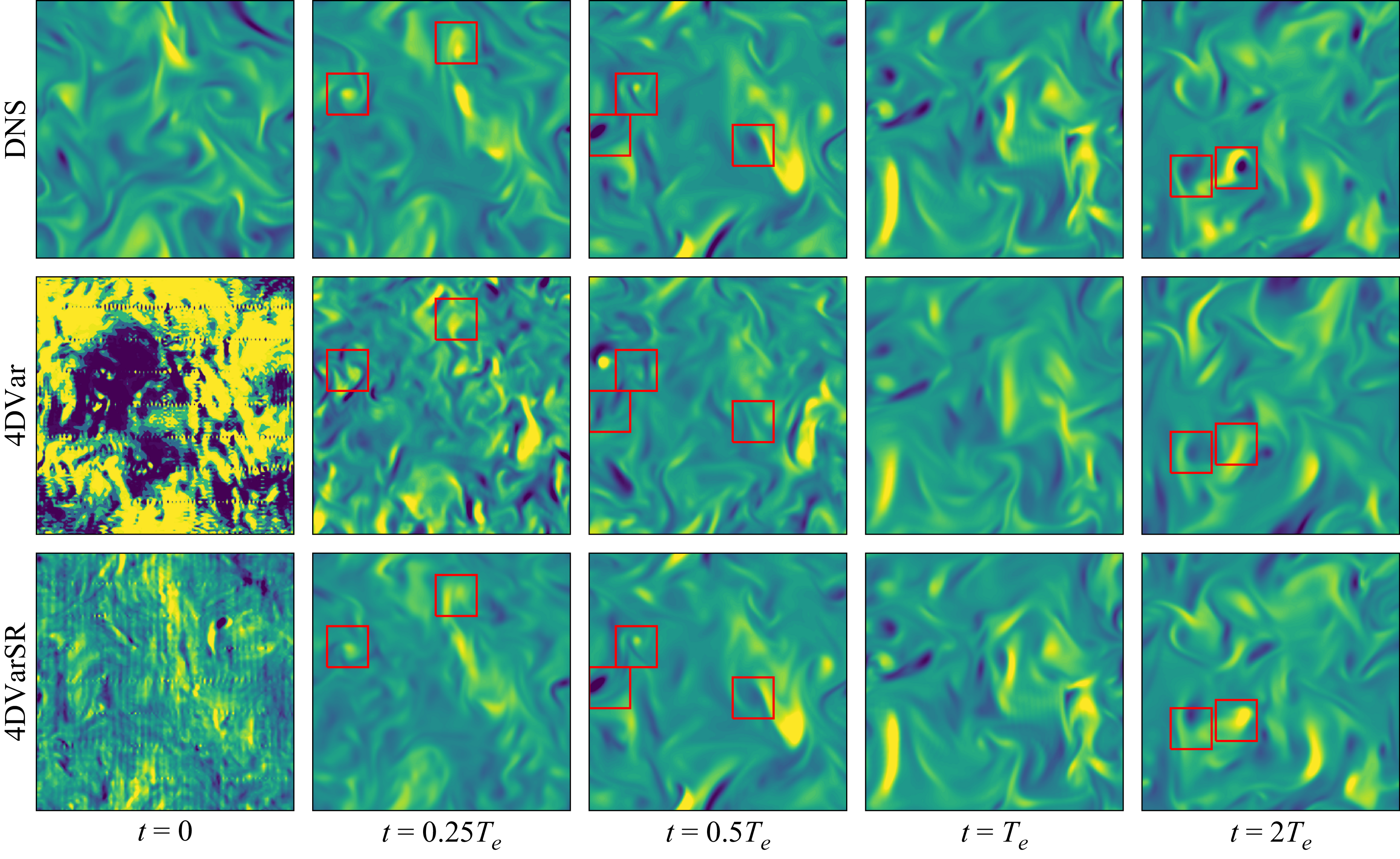


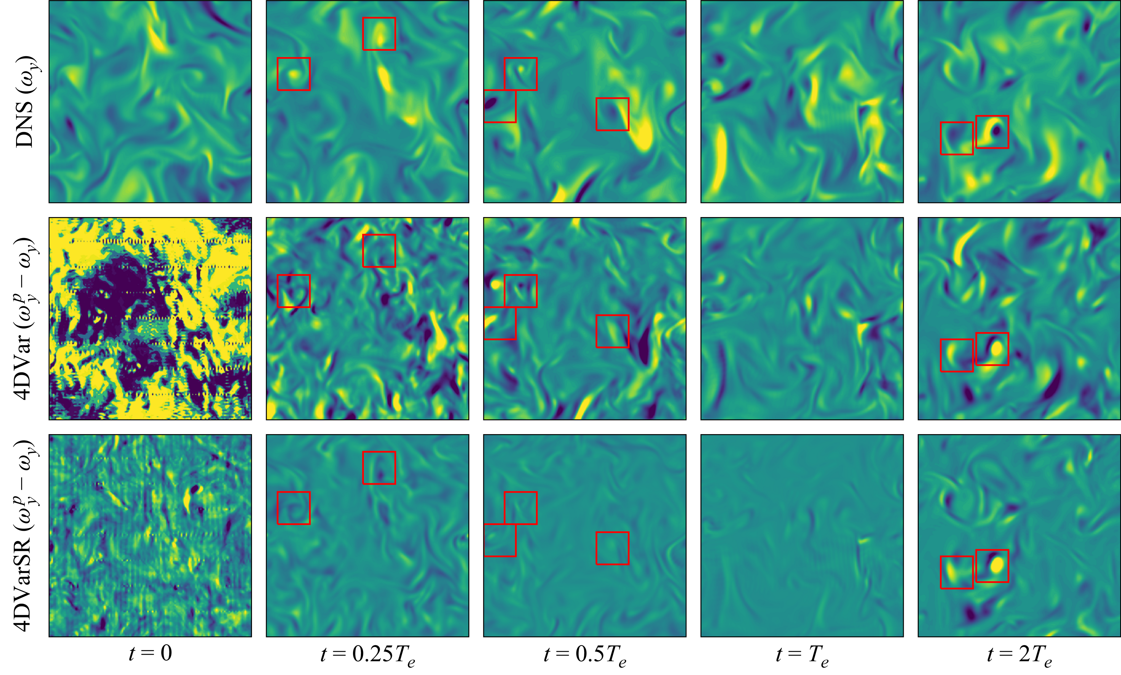


 Open access