





1. Introduction
The reflection of an incident shock over a reflecting surface is an important phenomenon in steady supersonic flow and has received a considerable amount of attention in studies since 1970s (see for instance Ben-Dor Reference Ben-Dor2007). The critical condition at which regular reflection (RR) or Mach reflection (MR) occurs is one of the important issues that have been studied.
There are two classical transition criteria, the detachment condition and the von Neumann condition (von Neumann Reference Von Neumann1943). For a given inflow Mach number (denoted $M_{0}$
in this paper), if the wedge angle (denoted
$M_{0}$
in this paper), if the wedge angle (denoted $\theta _{w}$
in this paper), i.e. the deflection angle of the wedge generating the incident shock wave, is larger than the detachment condition (denoted
$\theta _{w}$
in this paper), i.e. the deflection angle of the wedge generating the incident shock wave, is larger than the detachment condition (denoted $ \theta _{w}^{(D)}(M_{0})$
), then we necessarily have MR. If the wedge angle is smaller than the von Neumann condition (denoted
$ \theta _{w}^{(D)}(M_{0})$
), then we necessarily have MR. If the wedge angle is smaller than the von Neumann condition (denoted $\theta _{w}^{(N)}(M_{0})$
), then we necessarily have RR. Note that inverted MR that corresponds to MR below the von Neumann condition (Henderson & Lozzi Reference Henderson and Lozzi1979; Hornung Reference Hornung1986; Hekiri & Emanuel Reference Hekiri and Emanuel2015) may occur when there are additional influences such as downstream body (Roye et al. Reference Roye, Henderson and Menikoff1998), high downstream pressure (Ben-Dor et al. Reference Ben-Dor, Elperin, Li and Vasiliev1999), asymmetry shock reflection (Li et al. Reference Li, Chpoun and Ben-Dor1999) or a downstream incident shock (Guan et al. Reference Guan, Bai and Wu2018), but this inverted MR will not be considered here.
$\theta _{w}^{(N)}(M_{0})$
), then we necessarily have RR. Note that inverted MR that corresponds to MR below the von Neumann condition (Henderson & Lozzi Reference Henderson and Lozzi1979; Hornung Reference Hornung1986; Hekiri & Emanuel Reference Hekiri and Emanuel2015) may occur when there are additional influences such as downstream body (Roye et al. Reference Roye, Henderson and Menikoff1998), high downstream pressure (Ben-Dor et al. Reference Ben-Dor, Elperin, Li and Vasiliev1999), asymmetry shock reflection (Li et al. Reference Li, Chpoun and Ben-Dor1999) or a downstream incident shock (Guan et al. Reference Guan, Bai and Wu2018), but this inverted MR will not be considered here.
There is a dual-solution domain in the plane $(M_{0},\theta _{w})$
, since the detachment condition (
$(M_{0},\theta _{w})$
, since the detachment condition ( $\theta _{w}$ $=\theta _{w}^{(D)}(M_{0})$
) is above the von Neumann condition (
$=\theta _{w}^{(D)}(M_{0})$
) is above the von Neumann condition ( $\theta _{w}$ $=\theta _{w}^{(N)}(M_{0})$
). This means that when
$=\theta _{w}^{(N)}(M_{0})$
). This means that when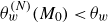 $\theta _{w}^{(N)}(M_{0})\lt \theta _{w}$ $\lt \theta _{w}^{(D)}(M_{0})$
, both RR and MR are possible. Although such a dual solution was recognised to be theoretically possible, great efforts have been required to clarify the real transition process.
$\lt \theta _{w}^{(D)}(M_{0})$
, both RR and MR are possible. Although such a dual solution was recognised to be theoretically possible, great efforts have been required to clarify the real transition process.
Early studies only observed MR (cf. Henderson & Lozzi Reference Henderson and Lozzi1975; Hornung et al. Reference Hornung, Oertel and Sandeman1979). The failure to observe RR led Hornung & Robinson (Reference Hornung and Robinson1982) to the conjecture that RR is unstable in the dual-solution domain. However, the stability analyses conducted by Teshukov (Reference Teshukov1989) and Li & Ben-Dor (Reference Li and Ben-Dor1996) proved that RR should be stable. In fact, Hornung et al. (Reference Hornung, Oertel and Sandeman1979) hypothesised a hysteresis process, which means that, in the dual-solution domain, whether we have MR or RR depends on the history of the building of the actual steady flow. Then RR was observed numerically (Vuillon et al. Reference Vuillon, Zeitoun and Ben-Dor1995) and experimentally (Chpoun et al. Reference Chpoun, Passerel, Li and Ben-Dor1995), where hysteresis occurs by changing the wedge angle. Later on a similar hysteresis was observed when the inflow Mach number changed from different directions (Ivanov et al. Reference Ivanov, Ben-Dor, Elperin, Kudryavtsev and Khotyanovsky2001). More discussions about this hysteresis can be found in the papers of Ben-Dor et al. (Reference Ben-Dor, Ivanov, Vasilev and Elperin2002) and Hornung (Reference Hornung2014).
Apart from transition at the inflow Mach number or wedge angle crossing the boundaries of the dual-solution domain, dynamic transition within the dual-solution domain is also possible. For instance, RR may transit to MR if the amplitude of the disturbance exceeds a certain level, according to a number of studies (cf. Ivanov et al. Reference Ivanov, Klemenkov, Kudryavtsev, Fomin and Kharitonov1997, Reference Ivanov, Markelov, Kudryavtsev and Gimelshein1998, Reference Ivanov, Kudryavtsev and Khotyanovskii2000; Kudryavtsev et al. Reference Kudryavtsev, Khotyanovsky, Ivanov and Vandromme2002; Li et al. Reference Li, Gao and Wu2011).
In the 1990s, it was discovered that stable MR is also subjected to geometric constraint. Vuillon et al. (Reference Vuillon, Zeitoun and Ben-Dor1995) studied shock reflection for extremely low and large values of the trailing-edge height $H_{R}$
(the distance of the wedge trailing edge (R) from the reflecting surface). Based on theoretical considerations, they found that the distance
$H_{R}$
(the distance of the wedge trailing edge (R) from the reflecting surface). Based on theoretical considerations, they found that the distance $H_{R}$
is bounded by a lower limit
$H_{R}$
is bounded by a lower limit $H_{R,min }$
and an upper limit
$H_{R,min }$
and an upper limit $H_{R,max }$
. According to Vuillon et al. (Reference Vuillon, Zeitoun and Ben-Dor1995), the lower limit corresponds to the case in which the reflected shock wave (r) grazes the trailing edge (R). The upper limit is determined by the point where the leading characteristic of the trailing-edge expansion fan (denoted TEF) intersects the incident shock wave at the reflection point (G) for RR and at the triple point (T) for MR.
$H_{R,max }$
. According to Vuillon et al. (Reference Vuillon, Zeitoun and Ben-Dor1995), the lower limit corresponds to the case in which the reflected shock wave (r) grazes the trailing edge (R). The upper limit is determined by the point where the leading characteristic of the trailing-edge expansion fan (denoted TEF) intersects the incident shock wave at the reflection point (G) for RR and at the triple point (T) for MR.
Consider first the upper limit. Vuillon et al. (Reference Vuillon, Zeitoun and Ben-Dor1995) supposed that MR may transit to RR (Vuillon et al. Reference Vuillon, Zeitoun and Ben-Dor1995) for $H_{R}\lt H_{R,max }$
, while Li & Ben-Dor (Reference Li and Ben-Dor1997) found that this transition occurs for
$H_{R}\lt H_{R,max }$
, while Li & Ben-Dor (Reference Li and Ben-Dor1997) found that this transition occurs for $H_{R}\gt H_{R,max }$
. Grasso & Paoli (Reference Grasso and Paoli1999) studied the effect of the geometrical set-up when accounting for shock reflection in non-equilibrium flow. Bai (Reference Bai2023) then provided the condition of
$H_{R}\gt H_{R,max }$
. Grasso & Paoli (Reference Grasso and Paoli1999) studied the effect of the geometrical set-up when accounting for shock reflection in non-equilibrium flow. Bai (Reference Bai2023) then provided the condition of $H_{R}$
at which MR transits to RR, and found that, beyond
$H_{R}$
at which MR transits to RR, and found that, beyond $H_{R}=H_{R,max }$
, the Mach stem height decreases nonlinearly with the trailing-edge height, until it vanishes at this new critical condition. Baby et al. (Reference Baby, Paramanantham and Rajesh2024) studied the role of the interference between the trailing-edge expansion fan and the incident shock (occurring for a short wedge, or
$H_{R}=H_{R,max }$
, the Mach stem height decreases nonlinearly with the trailing-edge height, until it vanishes at this new critical condition. Baby et al. (Reference Baby, Paramanantham and Rajesh2024) studied the role of the interference between the trailing-edge expansion fan and the incident shock (occurring for a short wedge, or $ H_{R}\gt H_{R,max }$
) in the transition criteria between RR and MR. He & Shi (Reference He and Shi2025) studied the steady MR structure and the time evolution of transition from RR to MR under velocity perturbation, for
$ H_{R}\gt H_{R,max }$
) in the transition criteria between RR and MR. He & Shi (Reference He and Shi2025) studied the steady MR structure and the time evolution of transition from RR to MR under velocity perturbation, for $H_{R}\gt H_{R,max }$
.
$H_{R}\gt H_{R,max }$
.
Now consider the shock reflection configuration at $H_{R}=H_{R,min }$
and this reflection configuration is schematically displayed in figure 1(a) for RR and figure 1(b) for MR. Vuillon et al. (Reference Vuillon, Zeitoun and Ben-Dor1995) pointed out that, whenever the distance
$H_{R}=H_{R,min }$
and this reflection configuration is schematically displayed in figure 1(a) for RR and figure 1(b) for MR. Vuillon et al. (Reference Vuillon, Zeitoun and Ben-Dor1995) pointed out that, whenever the distance $H_{R}$
reaches or is reduced below
$H_{R}$
reaches or is reduced below $H_{R,min }$
, the MR becomes unstable and its Mach stem moves upstream until the MR vanishes and a bow shock wave is established ahead of the leading edge of the reflecting wedge. As a result, the flow through the two-dimensional converging nozzle, formed by the surface of the reflecting wedge and the line of symmetry, becomes subsonic. The two-dimensional converging nozzle which is formed by the wedge and bottom surfaces is said to be unstarted or choked. This process was indeed observed not only by their numerical simulations but also in experiments (Chpoun et al. Reference Chpoun, Passerel, Li and Ben-Dor1995).
$H_{R,min }$
, the MR becomes unstable and its Mach stem moves upstream until the MR vanishes and a bow shock wave is established ahead of the leading edge of the reflecting wedge. As a result, the flow through the two-dimensional converging nozzle, formed by the surface of the reflecting wedge and the line of symmetry, becomes subsonic. The two-dimensional converging nozzle which is formed by the wedge and bottom surfaces is said to be unstarted or choked. This process was indeed observed not only by their numerical simulations but also in experiments (Chpoun et al. Reference Chpoun, Passerel, Li and Ben-Dor1995).
Shock reflection for $H_{R}=H_{R,min }$
at which the reflecting shock intersects the trailing edge
$H_{R}=H_{R,min }$
at which the reflecting shock intersects the trailing edge $R$
. Panels show (a) RR, (b) MR.
$R$
. Panels show (a) RR, (b) MR.

Li & Ben-Dor (Reference Li and Ben-Dor1997) stated that $H_{R,min }^{{\small (RR)}}$
(lower limit for RR) is smaller than
$H_{R,min }^{{\small (RR)}}$
(lower limit for RR) is smaller than $H_{R,min }^{(\textit{MR})}$
(lower limit for MR). If
$H_{R,min }^{(\textit{MR})}$
(lower limit for MR). If $ H_{R,min }^{{\small (RR)}}\lt$ $H_{R,min }^{(\textit{MR})}$
, then
$H_{R,min }^{(\textit{MR})}$
, then $H_{R,min }^{(RR)}\lt H_{R}$ $\lt H_{R,min }^{(\textit{MR})}$
defines a dual-solution stability range, which means that, when
$\lt H_{R,min }^{(\textit{MR})}$
defines a dual-solution stability range, which means that, when $H_{R,min }^{(RR)}\lt H_{R}$ $\lt H_{R,min }^{(\textit{MR})}$
, RR is stable and MR is unstable. We call
$\lt H_{R,min }^{(\textit{MR})}$
, RR is stable and MR is unstable. We call $H_{R,min }^{(RR)}$
and
$H_{R,min }^{(RR)}$
and $ H_{R,min }^{(\textit{MR})}$
the subcritical threshold and supercritical threshold for the geometric set-up, and call
$ H_{R,min }^{(\textit{MR})}$
the subcritical threshold and supercritical threshold for the geometric set-up, and call $\Delta H_{R,min }=$ $H_{R,min }^{(\textit{MR})}$ $-H_{R,min }^{(RR)}$
the dual-solution stability gap, which measures the width of the dual-solution stability range.
$-H_{R,min }^{(RR)}$
the dual-solution stability gap, which measures the width of the dual-solution stability range.
There are three issues which deserve further study. First, there lacks a formal proof for the inequality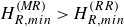 $H_{R,min }^{(\textit{MR})}\gt H_{R,min }^{(RR)}$
within the dual-solution domain. The existence of the Mach stem elevates the starting point of the reflected shock, but the reflected shock for MR has a smaller shock angle than that for RR; it is yet unknown whether these two counter-acting factors yield
$H_{R,min }^{(\textit{MR})}\gt H_{R,min }^{(RR)}$
within the dual-solution domain. The existence of the Mach stem elevates the starting point of the reflected shock, but the reflected shock for MR has a smaller shock angle than that for RR; it is yet unknown whether these two counter-acting factors yield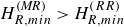 $H_{R,min }^{(\textit{MR})}\gt H_{R,min }^{(RR)}$
or
$H_{R,min }^{(\textit{MR})}\gt H_{R,min }^{(RR)}$
or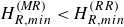 $ H_{R,min }^{(\textit{MR})}\lt H_{R,min }^{(RR)}$
. A formal proof is useful to clarify this question. Second, there lacks a quantitatively correct method to estimate the gap
$ H_{R,min }^{(\textit{MR})}\lt H_{R,min }^{(RR)}$
. A formal proof is useful to clarify this question. Second, there lacks a quantitatively correct method to estimate the gap $\Delta H_{R,min }=$ $H_{R,min }^{(\textit{MR})}$ $-H_{R,min }^{(RR)}$
. Third, the inequality
$-H_{R,min }^{(RR)}$
. Third, the inequality $H_{R,min }^{(\textit{MR})}\gt H_{R,min }^{(RR)}$
implies a new transition scenario, called the stable to unstable dynamic transition, not studied before: for
$H_{R,min }^{(\textit{MR})}\gt H_{R,min }^{(RR)}$
implies a new transition scenario, called the stable to unstable dynamic transition, not studied before: for $H_{R}$
satisfying
$H_{R}$
satisfying $H_{R,min }^{(RR)}\lt H_{R}$ $\lt H_{R,min }^{(\textit{MR})}$
, RR is stable while MR is unstable (in the sense that the flow will be unstarted or chocked, as pointed out by Vuillon et al. Reference Vuillon, Zeitoun and Ben-Dor1995).
$\lt H_{R,min }^{(\textit{MR})}$
, RR is stable while MR is unstable (in the sense that the flow will be unstarted or chocked, as pointed out by Vuillon et al. Reference Vuillon, Zeitoun and Ben-Dor1995).
This study addresses these three issues within the context of a two-dimensional inviscid flow.
The proof of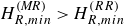 $H_{R,min }^{(\textit{MR})}\gt H_{R,min }^{(RR)}$
is difficult since
$H_{R,min }^{(\textit{MR})}\gt H_{R,min }^{(RR)}$
is difficult since $ H_{R,min }^{(\textit{MR})}$
involves the unknown Mach stem height
$ H_{R,min }^{(\textit{MR})}$
involves the unknown Mach stem height $H_{T}$
(see figure 1
b). In § 2, we use the method of transitivity to prove the inequality
$H_{T}$
(see figure 1
b). In § 2, we use the method of transitivity to prove the inequality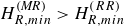 $H_{R,min }^{(\textit{MR})}\gt H_{R,min }^{(RR)}$
formally, for part of the dual-solution domain. The intermediate value in transitivity proof is a lower bound related to the minimum possible Mach stem height.
$H_{R,min }^{(\textit{MR})}\gt H_{R,min }^{(RR)}$
formally, for part of the dual-solution domain. The intermediate value in transitivity proof is a lower bound related to the minimum possible Mach stem height.
There is also a difficulty in finding the quantitatively correct values of $ H_{R,min }^{(\textit{MR})}$
and
$ H_{R,min }^{(\textit{MR})}$
and $\Delta H_{R,min }$
, since the height
$\Delta H_{R,min }$
, since the height $H_{R,min }^{(\textit{MR})}$
involves the unknown Mach stem height (
$H_{R,min }^{(\textit{MR})}$
involves the unknown Mach stem height ( $H_{T}$
). In § 3, we propose a roadmap to find
$H_{T}$
). In § 3, we propose a roadmap to find $H_{R,min }^{(\textit{MR})}$
and
$H_{R,min }^{(\textit{MR})}$
and $\Delta H_{R,min }$
. In the case that the Mach stem height varies linearly with respect to
$\Delta H_{R,min }$
. In the case that the Mach stem height varies linearly with respect to $H_{R}$
, we derive an explicit formula for the dual-solution gap, by which
$H_{R}$
, we derive an explicit formula for the dual-solution gap, by which $H_{R,min }^{(\textit{MR})}$
and
$H_{R,min }^{(\textit{MR})}$
and $\Delta H_{R,min }$
can be determined correctly once the coefficients of the linear formula for Mach stem height are provided through, for instance, high fidelity numerical simulation.
$\Delta H_{R,min }$
can be determined correctly once the coefficients of the linear formula for Mach stem height are provided through, for instance, high fidelity numerical simulation.
In § 4, we study the third issue, steady to unsteady dynamic transition, using numerical simulation. We will demonstrate that, with the dual-solution stability gap, if the stable RR is subjected to large-amplitude disturbance, then this stable RR may transit dynamically to unstable MR, a phenomenon that appears to have not been mentioned before. Specifically, with a particular condition lying inside the dual-solution stability gap, we perform numerical simulation of the dynamic transition, to demonstrate this new type of dynamic transition. The results of this numerical study, including how to set up the perturbation and how the shock structure evolves in time to have the transition, will be given. This not only confirms the existence of the dual-solution stability gap, but also shows how the transition evolves dynamically and depends on the upstream disturbance.
Some results will be presented in terms of the relative trailing-edge height $g$
defined by
$g$
defined by
 \begin{align} g=\frac {H_{R}}{H_{A}}. \end{align}
In terms of $g$
, the lower limit is defined by
$g$
, the lower limit is defined by
 \begin{equation} g_{\textit{min}}=\frac {H_{R,min }}{H_{A}} \end{equation}
and the dual-solution stability gap is defined by
 \begin{equation} \Delta g_{\textit{min}}=g_{\textit{min}}^{(\textit{MR})}-g_{\textit{min}}^{(RR)} ,\end{equation}
where $g_{\textit{min}}^{(RR)}$
is
$g_{\textit{min}}^{(RR)}$
is $g_{\textit{min}}$
for RR, and
$g_{\textit{min}}$
for RR, and $ g_{\textit{min}}^{(\textit{MR})}$
is
$ g_{\textit{min}}^{(\textit{MR})}$
is $g_{\textit{min}}$
for MR. The parameter
$g_{\textit{min}}$
for MR. The parameter $g$
is linked to the length of the wedge lower surface (figure 1
a) by the following obvious geometric relation:
$g$
is linked to the length of the wedge lower surface (figure 1
a) by the following obvious geometric relation:
 \begin{equation} \ w=\frac {H_{A}-H_{R}}{\sin \theta _{w}}=\frac {1-g}{\sin \theta _{w}}H_{A} \end{equation}
At $H_{R}=H_{R,min }$
, expression (1.4) gives
$H_{R}=H_{R,min }$
, expression (1.4) gives $w=w_{\textit{min}}$
, with
$w=w_{\textit{min}}$
, with
 \begin{equation} w_{\textit{min}}=\frac {H_{A}-H_{R,min }}{\sin \theta _{w}}=\frac {1-g_{\textit{min}}}{\sin \theta _{w}}H_{A}\text{.} \end{equation}
2. Proof of the inequality $g_{\textit{min}}^{(\textit{MR})}\gt g_{\textit{min}}^{(RR)}$
by transitivity
$g_{\textit{min}}^{(\textit{MR})}\gt g_{\textit{min}}^{(RR)}$
by transitivity

To prove the inequality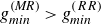 $g_{\textit{min}}^{(\textit{MR})}\gt g_{\textit{min}}^{(RR)}$
or
$g_{\textit{min}}^{(\textit{MR})}\gt g_{\textit{min}}^{(RR)}$
or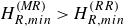 $H_{R,min }^{(\textit{MR})}\gt H_{R,min }^{(RR)}$
, we use the method of transitivity. For this purpose, we need an intermediate value
$H_{R,min }^{(\textit{MR})}\gt H_{R,min }^{(RR)}$
, we use the method of transitivity. For this purpose, we need an intermediate value $g_{\textit{min}}^{(int)}$
between
$g_{\textit{min}}^{(int)}$
between $g_{\textit{min}}^{(\textit{MR})}$
and
$g_{\textit{min}}^{(\textit{MR})}$
and $\ g_{\textit{min}}^{(RR)}$
, satisfying
$\ g_{\textit{min}}^{(RR)}$
, satisfying $g_{\textit{min}}^{(\textit{MR})}\gt g_{\textit{min}}^{(int)}\gt g_{\textit{min}}^{(RR)}$
. Here, we derive a lower bound
$g_{\textit{min}}^{(\textit{MR})}\gt g_{\textit{min}}^{(int)}\gt g_{\textit{min}}^{(RR)}$
. Here, we derive a lower bound $g_{\textit{min}}=g_{\textit{min}}^{(LB)}$
and use this lower bound as the intermediate value. This lower bound corresponds to the minimum Mach stem height.
$g_{\textit{min}}=g_{\textit{min}}^{(LB)}$
and use this lower bound as the intermediate value. This lower bound corresponds to the minimum Mach stem height.
2.1.
A lower bound for
$g_{\textit{min}}^{(\textit{MR})}$
corresponding to the minimum Mach stem height

Now, we derive a lower bound which can be used as an intermediate value to prove the inequality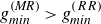 $g_{\textit{min}}^{(\textit{MR})}\gt g_{\textit{min}}^{(RR)}$
or
$g_{\textit{min}}^{(\textit{MR})}\gt g_{\textit{min}}^{(RR)}$
or $H_{R,min }^{(\textit{MR})}\gt H_{R,min }^{(RR)}$
through transitivity.
$H_{R,min }^{(\textit{MR})}\gt H_{R,min }^{(RR)}$
through transitivity.
Consider MR at $H_{R}=H_{R,min }$
, as shown in figure 2. The slipline from the triple point
$H_{R}=H_{R,min }$
, as shown in figure 2. The slipline from the triple point $T$
intersects the leading characteristic line of the trailing-edge expansion fan at point O. The tangent of the slipline at the triple point intersects the leading characteristic line of the trailing-edge expansion fan at point
$T$
intersects the leading characteristic line of the trailing-edge expansion fan at point O. The tangent of the slipline at the triple point intersects the leading characteristic line of the trailing-edge expansion fan at point $N^{\prime }$
.
$N^{\prime }$
.
Schematic display for MR with various notations needed in the proof. The minimum Mach stem height ( $H_{NT}$
) is the Mach stem height at
$H_{NT}$
) is the Mach stem height at $H_{N}=0$
.
$H_{N}=0$
.

Let the height of $N^{\prime }$
with respect to the reflecting surface be
$N^{\prime }$
with respect to the reflecting surface be $ H_{N^{\prime }}$
. The Mach stem height
$ H_{N^{\prime }}$
. The Mach stem height $H_{T}$
can be considered as composed of two segments
$H_{T}$
can be considered as composed of two segments
 \begin{equation} H_{T}=H_{TN}+H_{N} ,\end{equation}
where $H_{N}=H_{N^{\prime }}$
, so
$H_{N}=H_{N^{\prime }}$
, so
 \begin{align} H_{T}=H_{TN}+H_{N^{\prime }}. \end{align}
Using the geometric relations displayed in figure 2, it can be shown that the condition such that the reflected shock grazes the trailing edge leads to
 \begin{equation} \frac {{{H_{A1}}-}H_{TN}}{{\tan {\beta _{01}}}}+\frac {H_{R1}{-{H_{TN}}}}{{ \tan (\beta _{12}^{MR}-{\theta _{w}})}}=\frac {{{H_{A1}}-{H_{R1}}}}{{\tan { \theta _{w}}}} .\end{equation}
The total length of the horizontal line MN’, where M is the intersection of the line NN’ and the vertical line passing the vertex A, is equal to the wedge horizontal length plus the horizontal projection of the leading characteristic line RN’, so
 \begin{equation} \frac {{{H_{A1}}-}H_{TN}}{{\tan {\beta _{01}}}}+\frac {H_{TN}}{{\tan {\delta _{s}}}}=\frac {{{H_{A1}}-{H_{R1}}}}{{\tan {\theta _{w}}}}+\frac {{{H_{R1}}}}{{ \tan ({\mu _{2}}+{\delta _{s}})}} ,\end{equation}
where ${{\mu _{2}=\arcsin }}({1}/{M_{2}})$
is the Mach angle of the leading characteristics of the trailing-edge expansion fan and
${{\mu _{2}=\arcsin }}({1}/{M_{2}})$
is the Mach angle of the leading characteristics of the trailing-edge expansion fan and ${\delta _{s}}$
is the slipline angle as marked in figure 2.
${\delta _{s}}$
is the slipline angle as marked in figure 2.
Eliminating $H_{TN}$
in (2.3) and (2.4) gives the following expression for
$H_{TN}$
in (2.3) and (2.4) gives the following expression for $ {{{H_{R1}}}}/{{{H_{A1}}}}$
:
$ {{{H_{R1}}}}/{{{H_{A1}}}}$
:
 \begin{equation} \frac {{{H_{R1}}}}{{{H_{A1}}}}=\frac {{\dfrac {\psi {{t_{2}}}}{{\sin {\theta _{w} }}}+\dfrac {{{t_{1}}}}{{\tan {\theta _{w}}}}-\tan {\delta _{s}}}}{{{t_{2}}+ \dfrac {\psi {{t_{2}}}}{{\sin {\theta _{w}}}}+\dfrac {{{t_{1}}}}{{\tan {\theta _{w}}}}-\dfrac {{{t_{1}}}}{{\tan ({\mu _{2}}+{\delta _{s}})}}}} ,\end{equation}
where ${t_{1}}=\tan {\beta _{01}}\tan {\delta _{s}}$
,
${t_{1}}=\tan {\beta _{01}}\tan {\delta _{s}}$
, ${t_{2}}=\tan {\beta _{01}}-\tan {\delta _{s}}$
and
${t_{2}}=\tan {\beta _{01}}-\tan {\delta _{s}}$
and $\psi$
is defined by
$\psi$
is defined by $\psi = ({\sin (\beta _{12}^{MR}-\theta _{w})\sin (\beta _{01}-\theta _{w})})/({\sin (\beta _{01}+\beta _{12}^{MR}-\theta _{w})})$
. Here,
$\psi = ({\sin (\beta _{12}^{MR}-\theta _{w})\sin (\beta _{01}-\theta _{w})})/({\sin (\beta _{01}+\beta _{12}^{MR}-\theta _{w})})$
. Here, $\beta _{12}^{MR}$
is the shock angle of the reflected shock and
$\beta _{12}^{MR}$
is the shock angle of the reflected shock and $\beta _{01}$
is the shock angle of the incident shock, and both shock angles can be determined by the triple point solution.
$\beta _{01}$
is the shock angle of the incident shock, and both shock angles can be determined by the triple point solution.
According to (1.2), we have
 \begin{equation} g_{\textit{min}}^{MR}=\frac {{{H_{R1}}+H}_{N}}{{{H_{A1}}+H}_{N}} .\end{equation}
Since $H_{N}\gt 0$
, we have
$H_{N}\gt 0$
, we have
 \begin{equation} g_{\textit{min}}^{MR}\gt g_{\textit{min}}^{(LB)} ,\end{equation}
where
 \begin{equation} g_{\textit{min}}^{(LB)}=\frac {{{H_{R1}}}}{{{H_{A1}}}} \end{equation}
is the lower bound of $g_{\textit{min}}^{MR}$
. Here,
$g_{\textit{min}}^{MR}$
. Here, $ {{{H_{R1}}}}/{{{H_{A1}}}}$
is given by (2.5).
$ {{{H_{R1}}}}/{{{H_{A1}}}}$
is given by (2.5).
2.2.
Proof of
$g_{\textit{min}}^{(\textit{MR})}\gt g_{\textit{min}}^{(LB)}\gt g_{\textit{min}}^{(RR)}$

For RR (see figure 1 a), Li & Ben-Dor (Reference Li and Ben-Dor1997) give
 \begin{equation} H_{R,min }^{(RR)}=\phi ^{RR}w ,\end{equation}
with
 \begin{equation} \phi ^{RR}=\frac {\sin (\beta _{12}^{RR}-\theta _{w})\sin (\beta _{01}-\theta _{w})}{\sin (\beta _{01}+\beta _{12}^{RR}-\theta _{w})}\text{.} \end{equation}
Here, $\beta _{12}^{RR}$
is the shock angle of the reflected shock.
$\beta _{12}^{RR}$
is the shock angle of the reflected shock.
At $H_{R}=H_{R,min }^{(RR)}$
, we have
$H_{R}=H_{R,min }^{(RR)}$
, we have $w=w_{\textit{min}}$
where
$w=w_{\textit{min}}$
where $w_{\textit{min}}$
is given by (1.5). Thus (2.9) should be replaced by
$w_{\textit{min}}$
is given by (1.5). Thus (2.9) should be replaced by
 \begin{align} H_{R,min }^{(RR)}=\phi ^{RR}w_{\textit{min}} ,\end{align}
and, when (1.5) is used, we get
 \begin{align} g_{\textit{min}}^{(RR)}=\phi ^{RR}\frac {1-g_{\textit{min}}^{(RR)}}{\sin \theta _{w}} ,\end{align}
which can be solved to give
 \begin{equation} g_{\textit{min}}^{(RR)}=\frac {\phi ^{RR}}{\sin \theta _{w}+\phi ^{RR}}\text{.} \end{equation}
Once the lower bound $g_{\textit{min}}^{(LB)}$
is obtained by (2.8), we can get the relative lower bound
$g_{\textit{min}}^{(LB)}$
is obtained by (2.8), we can get the relative lower bound $\Delta g_{\textit{min}}^{(LB)}$
through
$\Delta g_{\textit{min}}^{(LB)}$
through
 \begin{equation} \Delta g_{\textit{min}}^{(LB)}=g_{\textit{min}}^{(LB)}-g_{\textit{min}}^{(RR)}\text{.} \end{equation}
The algorithm to find the lower bound $g_{\textit{min}}^{(LB)}$
involves flow parameters that are determined by shock wave relations. For this purpose, we first introduce the classical shock wave expressions.
$g_{\textit{min}}^{(LB)}$
involves flow parameters that are determined by shock wave relations. For this purpose, we first introduce the classical shock wave expressions.
We use $u$
to denote the upstream flow condition of an oblique shock wave, and
$u$
to denote the upstream flow condition of an oblique shock wave, and $d$
to denote the downstream flow condition. The shock angle
$d$
to denote the downstream flow condition. The shock angle $\beta _{ud}$
is related to the flow deflection angle
$\beta _{ud}$
is related to the flow deflection angle $\theta _{ud}$
through the shock angle relation
$\theta _{ud}$
through the shock angle relation
 \begin{equation} \tan \theta _{ud}=f_{\theta }(M_{u},\beta _{ud}) ,\end{equation}
where
 \begin{align} f_{\theta }(M,\beta)=\frac {2\left ( {M}^{2}{\sin }^{2}{\beta }-1\right) }{ \left ( {M}^{2}\left ( \gamma +\cos {2\beta }\right) +2\right) \tan {\beta }}. \end{align}
For given $M_{u}\gt 1$
and
$M_{u}\gt 1$
and $\theta _{ud}$
(below the detached angle), the relation (2.15) admits two solutions for
$\theta _{ud}$
(below the detached angle), the relation (2.15) admits two solutions for $\beta _{ud}$
; the smaller one is called the weak solution, and the larger one is the strong solution.
$\beta _{ud}$
; the smaller one is called the weak solution, and the larger one is the strong solution.
The Mach number $M_{u}$
is then given by the shock relation for Mach number
$M_{u}$
is then given by the shock relation for Mach number
 \begin{equation} M_{d}=f_{M}(M_{u},\beta _{ud}) ,\end{equation}
where
 \begin{align} f_{M}(M,{\beta)}=\sqrt {\frac {\left ( \gamma -1\right) {M}^{2}+2}{2\gamma {M} ^{2}{\sin }^{2}{\beta }-\left ( \gamma -1\right) }+\frac {2{M}^{2}{\cos }^{2}{ \beta }}{\left ( \gamma -1\right) {M}^{2}{\sin }^{2}{\beta }+2}} .\end{align}
Also, the pressure is given by the shock relation for pressure
 \begin{equation} p_{d}=p_{u}f_{p}(M_{u},\beta _{ud}) ,\end{equation}
where
 \begin{align} f_{p}(M,{\beta)}=1+\frac {2\gamma }{\gamma +1}\left ( {M}^{2}{\sin }^{2}{ \beta }-1\right). \end{align}
Now we outline the algorithm to find the lower bound $g_{\textit{min}}^{(LB)}$
.
$g_{\textit{min}}^{(LB)}$
.
Step 1. Consider any point $M_{0}$
and
$M_{0}$
and $\theta _{w}$
inside the dual-solution domain. Use the oblique wave expression to find the solution in region (1) of figure 2. Find the shock angle
$\theta _{w}$
inside the dual-solution domain. Use the oblique wave expression to find the solution in region (1) of figure 2. Find the shock angle $\beta _{01}$
by solving
$\beta _{01}$
by solving $\tan \theta _{w}=f_{\theta }(M_{0},\beta _{01})$
for the weak solution. Find
$\tan \theta _{w}=f_{\theta }(M_{0},\beta _{01})$
for the weak solution. Find $M_{1}$
and
$M_{1}$
and $ p_{1}$
by solving
$ p_{1}$
by solving $M_{1}=f_{M}(M_{0},\beta _{01})$
and
$M_{1}=f_{M}(M_{0},\beta _{01})$
and $ p_{1}=p_{0}f_{p}(M_{0},\beta _{01})$
Step 2. Find $g_{\textit{min}}^{RR}$
through (2.13). For this purpose, we first solve for the two shock theory for RR to find
$g_{\textit{min}}^{RR}$
through (2.13). For this purpose, we first solve for the two shock theory for RR to find $\beta _{_{12}}^{RR}$
. The shock angle
$\beta _{_{12}}^{RR}$
. The shock angle $\beta _{_{12}}^{RR}$
is obtained by solving
$\beta _{_{12}}^{RR}$
is obtained by solving $\tan \theta _{w}=f_{\theta }(M_{1},{\beta _{_{12}}^{RR}})$
for the weak solution. The expression (2.10) for
$\tan \theta _{w}=f_{\theta }(M_{1},{\beta _{_{12}}^{RR}})$
for the weak solution. The expression (2.10) for $\phi ^{RR}$
that appears in (2.13) can then be computed, so we obtain
$\phi ^{RR}$
that appears in (2.13) can then be computed, so we obtain $g_{\textit{min}}^{(RR)}$
through (2.13).
$g_{\textit{min}}^{(RR)}$
through (2.13).
Step 3. Find $g_{\textit{min}}^{(LB)}$
through (2.8). To do this, we first need to find the triple point solution. Using the flow parallel conditions
$g_{\textit{min}}^{(LB)}$
through (2.8). To do this, we first need to find the triple point solution. Using the flow parallel conditions $\theta _{12}=\theta _{w}-\delta _{s}$
,
$\theta _{12}=\theta _{w}-\delta _{s}$
, $\theta _{03}=\delta _{s}$
and the pressure balance relation
$\theta _{03}=\delta _{s}$
and the pressure balance relation $p_{3}^{MR}=p_{2}^{MR}$
, we solve
$p_{3}^{MR}=p_{2}^{MR}$
, we solve
 \begin{align} \tan \theta _{12}=f_{\theta }(M_{1},{\beta _{_{12}}^{MR}})\text{, } p_{2}^{MR}=p_{1}f_{p}(M_{1},\beta _{12}^{MR})\text{ (weak solution)} ,\end{align}
and
 \begin{equation} \tan \theta _{03}=f_{\theta }(M_{0},{\beta _{_{03}}^{MR}})\text{, } p_{3}^{MR}=p_{0}f_{p}(M_{0},\beta _{03}^{MR})\text{ (strong solution)} .\end{equation}
Then, (2.5) is used for $ {{{H_{R1}}}}/{{{H_{A1}}}}$
. Finally, we get
$ {{{H_{R1}}}}/{{{H_{A1}}}}$
. Finally, we get $g_{\textit{min}}^{(LB)}$
through (2.8).
$g_{\textit{min}}^{(LB)}$
through (2.8).
Step 4. Finally, we get $\Delta g_{\textit{min}}^{(LB)}$
through (2.14). For other
$\Delta g_{\textit{min}}^{(LB)}$
through (2.14). For other $M_{0}$
and
$M_{0}$
and $\theta _{w}$
, go to step 1 and repeat step 2 to step 4.
$\theta _{w}$
, go to step 1 and repeat step 2 to step 4.
The lower bound $\Delta g_{\textit{min}}^{(LB)}$
thus obtained for
$\Delta g_{\textit{min}}^{(LB)}$
thus obtained for $M_{0}$
and
$M_{0}$
and $ \theta _{w}$
lying inside the dual-solution domain is shown in figure 3. We see that
$ \theta _{w}$
lying inside the dual-solution domain is shown in figure 3. We see that $\Delta g_{\textit{min}}^{(LB)}$
is away from zero in the dual-solution domain except for the tip horn region (OPQ) which is near the left boundary of this dual-solution domain.
$\Delta g_{\textit{min}}^{(LB)}$
is away from zero in the dual-solution domain except for the tip horn region (OPQ) which is near the left boundary of this dual-solution domain.
Thus we have shown that the inequality $\Delta g_{\textit{min}}^{(LB)}\gt 0$
and thus
$\Delta g_{\textit{min}}^{(LB)}\gt 0$
and thus
 \begin{equation} g_{\textit{min}}^{(LB)}\gt g_{\textit{min}}^{(RR)} \end{equation}
holds within the dual-solution domain except in the tip horn region. Note that tip horn region is small.
Contourlines of the relative lower bound $\Delta g_{\textit{min}}^{(LB)}$
in the dual-solution domain. The tip horn region is defined as the region OPQ with
$\Delta g_{\textit{min}}^{(LB)}$
in the dual-solution domain. The tip horn region is defined as the region OPQ with $\Delta g_{\textit{min}}^{(LB)}\rightarrow 0$
.
$\Delta g_{\textit{min}}^{(LB)}\rightarrow 0$
.

By transitivity through (2.7) and (2.23), the inequality
 \begin{equation} g_{\textit{min}}^{(\textit{MR})}\gt g_{\textit{min}}^{(RR)} \end{equation}
holds and thus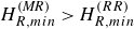 $H_{R,min }^{(\textit{MR})}\gt H_{R,min }^{(RR)}$
holds, within the dual-solution domain, except inside the tip horn region.
$H_{R,min }^{(\textit{MR})}\gt H_{R,min }^{(RR)}$
holds, within the dual-solution domain, except inside the tip horn region.
3. A method to determine the quantitative values of
$g_{\textit{min}}^{(\textit{MR})}$
and
$\Delta g_{\textit{min}}$


The lower bound of the dual-solution stability gap derived in § 2 has been used as an intermediate value for proof by transitivity. The real value of this gap should be greater than this lower bound. Here, we provide a method to derive the quantitative value of this gap once $M_{0}$
and
$M_{0}$
and $\theta _{w}$
are given.
$\theta _{w}$
are given.
3.1.
A road map to find
$g_{\textit{min}}^{(\textit{MR})}$
and
$\Delta g_{\textit{min}}$


For MR with Mach stem height $H_{T}$
(see figure 1
b), Li & Ben-Dor (Reference Li and Ben-Dor1997) give the following expression for
$H_{T}$
(see figure 1
b), Li & Ben-Dor (Reference Li and Ben-Dor1997) give the following expression for $H_{R,min }^{(\textit{MR})}$
:
$H_{R,min }^{(\textit{MR})}$
:
 \begin{equation} H_{R,min }^{(\textit{MR})}=H_{T}+\phi ^{MR}w ,\end{equation}
where
 \begin{equation} \phi ^{MR}=\frac {\sin (\beta _{12}^{MR}-\theta _{w})\sin (\beta _{01}-\theta _{w})}{\sin (\beta _{01}+\beta _{12}^{MR}-\theta _{w})}\text{.} \end{equation}
Here, $\beta _{12}^{MR}$
is the shock angle of the reflected shock in case of MR.
$\beta _{12}^{MR}$
is the shock angle of the reflected shock in case of MR.
However, (3.1) cannot be directly applied here. The reason is that $H_{T}=H_{T,min }$
and
$H_{T}=H_{T,min }$
and $w=w_{\textit{min}}$
(see (1.5) for
$w=w_{\textit{min}}$
(see (1.5) for $w_{\textit{min}}$
) at
$w_{\textit{min}}$
) at $H_{R}=H_{R,min }^{(\textit{MR})}$
, so expression (3.1) should be replaced by
$H_{R}=H_{R,min }^{(\textit{MR})}$
, so expression (3.1) should be replaced by
 \begin{equation} H_{R,min }^{(\textit{MR})}=H_{T,min }+\phi ^{MR}w_{\textit{min}} .\end{equation}
We define the relative Mach stem height as $h_{T}= {H_{T}}/{H_{A}}$
. Using
$h_{T}= {H_{T}}/{H_{A}}$
. Using $H_{T,min }=h_{T,min }H_{A}$
and (1.5) in (3.3), and replacing
$H_{T,min }=h_{T,min }H_{A}$
and (1.5) in (3.3), and replacing $H_{R,min }^{(\textit{MR})}$
by
$H_{R,min }^{(\textit{MR})}$
by $g_{\textit{min}}^{(\textit{MR})}H_{A}$
, we obtain the following expression for
$g_{\textit{min}}^{(\textit{MR})}H_{A}$
, we obtain the following expression for $g_{\textit{min}}^{(\textit{MR})}$
:
$g_{\textit{min}}^{(\textit{MR})}$
:
 \begin{equation} g_{\textit{min}}^{(\textit{MR})}=h_{T,min }+\frac {\phi ^{MR}}{\sin \theta _{w}}\left ( 1-g_{\textit{min}}^{(\textit{MR})}\right) ,\end{equation}
where $\phi ^{MR}$
is given by (3.2).
$\phi ^{MR}$
is given by (3.2).
According to Hornung & Robinson (Reference Hornung and Robinson1982), $ {H_{T}}/{w}=h ( M_{0},\theta _{w},( {H_{R}}/{w}))$
, which can be equivalently written as
$ {H_{T}}/{w}=h ( M_{0},\theta _{w},( {H_{R}}/{w}))$
, which can be equivalently written as
 \begin{equation} h_{T}=h_{T}\left ( M_{0},\theta _{w},g\right) \end{equation}
due to (1.4). Note that the functional form also depends on $\gamma$
, the ratio of the specific heats. Here, we do not consider varying
$\gamma$
, the ratio of the specific heats. Here, we do not consider varying $\gamma$
so this parameter is considered as a constant in (3.5).
$\gamma$
so this parameter is considered as a constant in (3.5).
Putting $g=g_{\textit{min}}^{(\textit{MR})}$
and
$g=g_{\textit{min}}^{(\textit{MR})}$
and $h_{T}=h_{T,min }$
in (3.5), we have
$h_{T}=h_{T,min }$
in (3.5), we have
 \begin{equation} h_{T,min }=h_{T}\left ( M_{0},\theta _{w},g_{\textit{min}}^{(\textit{MR})}\right) .\end{equation}
Since $h_{T,min }$
and
$h_{T,min }$
and $ {\phi ^{MR}}/{\sin \theta _{w}}$
are functions of
$ {\phi ^{MR}}/{\sin \theta _{w}}$
are functions of $M_{0}$
and
$M_{0}$
and $\theta _{w}$
, expression (3.4) means that
$\theta _{w}$
, expression (3.4) means that $g_{\textit{min}}^{(\textit{MR})}$
is a function of
$g_{\textit{min}}^{(\textit{MR})}$
is a function of $M_{0}$
and
$M_{0}$
and $\theta _{w}$
.
$\theta _{w}$
.
Then (3.4) can be solved for $g_{\textit{min}}^{(\textit{MR})}$
if we know expression (3.6).
$g_{\textit{min}}^{(\textit{MR})}$
if we know expression (3.6).
3.2.
Efficient method for
$g_{\textit{min}}^{(\textit{MR})}$
and
$\Delta g_{\textit{min}}$
when
$h_{T}$
is a linear function of
$g$


Li & Ben-Dor (Reference Li and Ben-Dor1997) stated that the calculations of Vuillon et al. (Reference Vuillon, Zeitoun and Ben-Dor1995) indicated that, within the forth-order approximation, the trajectory of the Mach stem foot (similar to point G in figure 1
b ) is a straight line, meaning that the Mach stem height may decrease linearly with $H_{R}$
. Schotz et al.(Reference Schotz, Levy, Ben-Dor and Igra1997, equation (21)) and Bai & Wu (Reference Bai and Wu2021) also suggested equivalent linear variation.
$H_{R}$
. Schotz et al.(Reference Schotz, Levy, Ben-Dor and Igra1997, equation (21)) and Bai & Wu (Reference Bai and Wu2021) also suggested equivalent linear variation.
Bai & Wu (Reference Bai and Wu2021) considered several conditions and showed, through high fidelity numerical simulation, that the relative Mach stem height can be fitted by a linear formula, i.e.
 \begin{equation} h_{T}=Ag+B \end{equation}
in terms of the present notations. The linear formula fits the numerical results with $R^{2}$
above
$R^{2}$
above $0.99$
, where
$0.99$
, where $R^{2}$
stands for the linear correlation coefficient.
$R^{2}$
stands for the linear correlation coefficient.
Only one condition considered by Bai & Wu (Reference Bai and Wu2021) lies within the dual-solution domain. Here, we added two more cases in the dual-solution domain, with $A$
and
$A$
and $B$
determined by numerical simulation using the Fluent package with the choice of second-order Roe scheme in the same way as Bai & Wu (Reference Bai and Wu2021) but we increase the number grid points in the horizontal direction since the geometry is longer in the present calculation. The condition by Bai & Wu (Reference Bai and Wu2021) and the two new cases are shown in table 1.
$B$
determined by numerical simulation using the Fluent package with the choice of second-order Roe scheme in the same way as Bai & Wu (Reference Bai and Wu2021) but we increase the number grid points in the horizontal direction since the geometry is longer in the present calculation. The condition by Bai & Wu (Reference Bai and Wu2021) and the two new cases are shown in table 1.
Note that Bai & Wu (Reference Bai and Wu2021) suggested the grid number after grid convergence study. Here, we follow the same approach and display in figure 4 the relative Mach stem heights obtained by numerical simulation with four different values of $g$
. The numerical results are marked with black circles, the additional marks in figure 4 show that numerical results with a grid of
$g$
. The numerical results are marked with black circles, the additional marks in figure 4 show that numerical results with a grid of $400\times 800$
points are acceptable since further refining the grid does not change the Mach stem height noticeably.
$400\times 800$
points are acceptable since further refining the grid does not change the Mach stem height noticeably.
Similarly to case 1 studied by Bai & Wu (Reference Bai and Wu2021), the normalised Mach stem height is almost linear with respect to $g$
. In figure 4, a straight line
$g$
. In figure 4, a straight line $e_{1}e_{2}$
is marked across the numerical data and this straight line is given by (3.7), with
$e_{1}e_{2}$
is marked across the numerical data and this straight line is given by (3.7), with $A$
and
$A$
and $B$
shown in table 1. For case 3, we also have similar behaviour and the fitted coefficients
$B$
shown in table 1. For case 3, we also have similar behaviour and the fitted coefficients $A$
and
$A$
and $B$
are shown in table 1. In all cases, the linear form (3.7) holds with
$B$
are shown in table 1. In all cases, the linear form (3.7) holds with $R^{2}\gt 0.99$
.
$R^{2}\gt 0.99$
.
The coefficients $A$
and
$A$
and $B$
for three cases. Case 1 is from Bai & Wu (Reference Bai and Wu2021). Case 2 is from the present calculation with
$B$
for three cases. Case 1 is from Bai & Wu (Reference Bai and Wu2021). Case 2 is from the present calculation with $g=0.45,0.50,0.55,0.60$
. Case 3 is from the present calculation with
$g=0.45,0.50,0.55,0.60$
. Case 3 is from the present calculation with $g=0.45,0.50,0.55,0.60$
.
$g=0.45,0.50,0.55,0.60$
.

Numerical results of the normalised Mach stem heights as functions of $g$
for case 2.The line
$g$
for case 2.The line $e_{1}e_{2}$
is a straight line passing through Computational Fluid Dynamics (CFD) data. Open circles are CFD data using different grids.
$e_{1}e_{2}$
is a straight line passing through Computational Fluid Dynamics (CFD) data. Open circles are CFD data using different grids.

In conditions such that the relative Mach stem height follows the linear form (3.7), we have
 \begin{equation} h_{T,min }=Ag_{\textit{min}}^{(\textit{MR})}+B \end{equation}
so that the expression (3.4) can be solved to give the following explicit expression for $g_{\textit{min}}^{(\textit{MR})}$
:
$g_{\textit{min}}^{(\textit{MR})}$
:
 \begin{equation} \overline {g}_{\textit{min}}^{{\small (MR)}}=\frac {\dfrac {\phi ^{MR}}{\sin \theta _{w}}+B}{1-A+\dfrac {\phi ^{MR}}{\sin \theta _{w}}}, \end{equation}
where $\overline {g}_{\textit{min}}^{(\textit{MR})}$
denotes
$\overline {g}_{\textit{min}}^{(\textit{MR})}$
denotes $g_{\textit{min}}^{(\textit{MR})}$
when (3.8) is applied.
$g_{\textit{min}}^{(\textit{MR})}$
when (3.8) is applied.
3.3.
Predicted values of
$\overline {g}_{\textit{min}}^{(\textit{MR})}$
and
$\triangle \overline {g}_{\textit{min}}$
for three cases


For a given condition ( $M_{0},\theta _{w}$
), if (3.7) holds and if the exact values of
$M_{0},\theta _{w}$
), if (3.7) holds and if the exact values of $A$
and
$A$
and $B$
are known (e.g. from high fidelity numerical simulation), then (3.9) yields the required values of
$B$
are known (e.g. from high fidelity numerical simulation), then (3.9) yields the required values of $g_{\textit{min}}^{(\textit{MR})}=\overline {g}_{\textit{min}}^{{\small (MR)}}$
, and hence the required values of
$g_{\textit{min}}^{(\textit{MR})}=\overline {g}_{\textit{min}}^{{\small (MR)}}$
, and hence the required values of $\triangle g_{\textit{min}}=\triangle \overline {g}_{\textit{min}}$
, where
$\triangle g_{\textit{min}}=\triangle \overline {g}_{\textit{min}}$
, where
 \begin{equation} \triangle \overline {g}_{\textit{min}}=\overline {g}_{\textit{min}}^{(\textit{MR})}-g_{\textit{min}}^{(RR)} ,\end{equation}
with $g_{\textit{min}}^{(RR)}$
computed by (2.13). The quantity
$g_{\textit{min}}^{(RR)}$
computed by (2.13). The quantity $g_{\textit{min}}^{(RR)}$
computed by the exact expression (2.13) is shown in figure 5.
$g_{\textit{min}}^{(RR)}$
computed by the exact expression (2.13) is shown in figure 5.
Contourlines of $g_{\textit{min}}^{(RR)}$
in the dual-solution domain. This value is given by the exact formula (2.13).
$g_{\textit{min}}^{(RR)}$
in the dual-solution domain. This value is given by the exact formula (2.13).

Table 2 gives $\overline {g}_{\textit{min}}^{(\textit{MR})}$
and
$\overline {g}_{\textit{min}}^{(\textit{MR})}$
and $\triangle \overline {g}_{\textit{min}}$
thus obtained.
$\triangle \overline {g}_{\textit{min}}$
thus obtained.
Predicted values of $\overline {g}_{\textit{min}}^{(\textit{MR})}$
and
$\overline {g}_{\textit{min}}^{(\textit{MR})}$
and $\triangle \overline {g}_{\textit{min}}$
for the three cases shown in table 1.
$\triangle \overline {g}_{\textit{min}}$
for the three cases shown in table 1.

Now let us give some details for case 1. Using (2.13), we get, for $M_{0}=4$
,
$M_{0}=4$
, $\theta _{w}=25^{o}$
,
$\theta _{w}=25^{o}$
,
 \begin{equation} g_{\textit{min}}^{(RR)}=0.239 .\end{equation}
With $A=-1.031$
and
$A=-1.031$
and $B=0.723$
from table 1, we get from (3.9) the value
$B=0.723$
from table 1, we get from (3.9) the value
 \begin{equation} \overline {g}_{\textit{min}}^{(\textit{MR})}=0.417 .\end{equation}
Hence, for case 1,
 \begin{align} \triangle \overline {g}_{\textit{min}}=0.178 .\end{align}
3.4. Numerical validation
Now we perform numerical simulation, using the same numerical approach as stated above, to check the predicted quantities of $\overline {g}_{\textit{min}}^{(\textit{MR})}$
and
$\overline {g}_{\textit{min}}^{(\textit{MR})}$
and $\triangle \overline {g}_{\textit{min}}$
. To do this, we seek a
$\triangle \overline {g}_{\textit{min}}$
. To do this, we seek a $g=g_{min,CFD}^{l}$
value near
$g=g_{min,CFD}^{l}$
value near $\overline {g}_{\textit{min}}^{(\textit{MR})}$
for which we get a unstable MR numerical solution, and a
$\overline {g}_{\textit{min}}^{(\textit{MR})}$
for which we get a unstable MR numerical solution, and a $g=g_{min,CFD}^{u}$
value near
$g=g_{min,CFD}^{u}$
value near $\overline {g}_{\textit{min}}^{(\textit{MR})}$
for which we get a stable MR numerical solution. Once
$\overline {g}_{\textit{min}}^{(\textit{MR})}$
for which we get a stable MR numerical solution. Once $g_{\textit{min} ,\textit{CFD}}^{u}$
is close to
$g_{\textit{min} ,\textit{CFD}}^{u}$
is close to $g_{\textit{min} ,\textit{CFD}}^{l}$
, we may say that
$g_{\textit{min} ,\textit{CFD}}^{l}$
, we may say that $g_{\textit{min}}^{(\textit{MR})}$
predicted by numerical simulation is
$g_{\textit{min}}^{(\textit{MR})}$
predicted by numerical simulation is
 \begin{align} g_{\textit{min} ,\textit{CFD}}=\frac {1}{2}(g_{\textit{min} ,\textit{CFD}}^{u}+g_{\textit{min} ,\textit{CFD}}^{l}). \end{align}
The difference between the predicted value $\overline {g}_{\textit{min}}^{(\textit{MR})}$
and
$\overline {g}_{\textit{min}}^{(\textit{MR})}$
and $g_{\textit{min} ,\textit{CFD}}$
is defined by
$g_{\textit{min} ,\textit{CFD}}$
is defined by
 \begin{align} \varepsilon =\frac {g_{\textit{min} ,\textit{CFD}}-\overline {g}_{\textit{min}}^{(\textit{MR})}}{\overline {g}_{\textit{min}}^{(\textit{MR})}} .\end{align}
The values of $g_{\textit{min} ,\textit{CFD}}^{l}$
,
$g_{\textit{min} ,\textit{CFD}}^{l}$
, $g_{\textit{min} ,\textit{CFD}}^{u},g_{\textit{min} ,\textit{CFD}}$
and
$g_{\textit{min} ,\textit{CFD}}^{u},g_{\textit{min} ,\textit{CFD}}$
and $\varepsilon$
are shown in table 3. The Mach number contourlines at
$\varepsilon$
are shown in table 3. The Mach number contourlines at $g=g_{\textit{min} ,\textit{CFD}}^{l}$
and
$g=g_{\textit{min} ,\textit{CFD}}^{l}$
and $g=$
$g=$ $g_{\textit{min} ,\textit{CFD}}^{u}$
are displayed in figures 6, 7 and 8 for cases 1, 2 and 3. Note that for
$g_{\textit{min} ,\textit{CFD}}^{u}$
are displayed in figures 6, 7 and 8 for cases 1, 2 and 3. Note that for $g=g_{\textit{min} ,\textit{CFD}}^{l}$
the flow is unstable, so figures 6(a), 7(a) and 8(a) are a snapshot of the time-dependent result.
$g=g_{\textit{min} ,\textit{CFD}}^{l}$
the flow is unstable, so figures 6(a), 7(a) and 8(a) are a snapshot of the time-dependent result.
The values of $g_{\textit{min} ,\textit{CFD}}^{l}$
,
$g_{\textit{min} ,\textit{CFD}}^{l}$
, $g_{\textit{min} ,\textit{CFD}}^{u}$
,
$g_{\textit{min} ,\textit{CFD}}^{u}$
, $g_{\textit{min} ,\textit{CFD}}$
and
$g_{\textit{min} ,\textit{CFD}}$
and $ \varepsilon$
for the three cases.
$ \varepsilon$
for the three cases.

According to table 3, $\overline {g}_{\textit{min}}^{(\textit{MR})}$
is very close to
$\overline {g}_{\textit{min}}^{(\textit{MR})}$
is very close to $g_{\textit{min} ,\textit{CFD}}$
, with a relative difference less than
$g_{\textit{min} ,\textit{CFD}}$
, with a relative difference less than $2\,\%$
. Consider for instance case 1, where the predicted value for
$2\,\%$
. Consider for instance case 1, where the predicted value for $g_{\textit{min}}^{(\textit{MR})}$
is
$g_{\textit{min}}^{(\textit{MR})}$
is $\overline {g}_{\textit{min}}^{(\textit{MR})}=0.417$
(see (3.12)), while the numerical simulation gives
$\overline {g}_{\textit{min}}^{(\textit{MR})}=0.417$
(see (3.12)), while the numerical simulation gives $g_{\textit{min} ,\textit{CFD}}$ $=0.4225\pm 0.0025$
. The difference is
$=0.4225\pm 0.0025$
. The difference is $\varepsilon =1.\, 32\,\% \pm 0.60\,\%$
. Note that
$\varepsilon =1.\, 32\,\% \pm 0.60\,\%$
. Note that $g_{\textit{min} ,\textit{CFD}}^{l}$
and
$g_{\textit{min} ,\textit{CFD}}^{l}$
and $g_{\textit{min} ,\textit{CFD}}^{u}$
are both (slightly) larger than
$g_{\textit{min} ,\textit{CFD}}^{u}$
are both (slightly) larger than $\overline {g}_{\textit{min}}^{(\textit{MR})}$
(possibly due to numerical error). For case 2 and case 3, we have
$\overline {g}_{\textit{min}}^{(\textit{MR})}$
(possibly due to numerical error). For case 2 and case 3, we have $g_{\textit{min} ,\textit{CFD}}^{l}\lt \overline {g}_{\textit{min}}^{(\textit{MR})}\lt$ $g_{\textit{min} ,\textit{CFD}}^{u}$
.
$g_{\textit{min} ,\textit{CFD}}^{u}$
.
Mach number contours for case 1: (a) $g=0.420$
, (b)
$g=0.420$
, (b) $g=0.425$
.
$g=0.425$
.

Mach number contours for case 2: (a) $g=0.440$
, (b)
$g=0.440$
, (b) $g=0.450$
.
$g=0.450$
.

Mach number contours for case 3: (a) $g=0.350$
, (b)
$g=0.350$
, (b) $g=0.360$
.
$g=0.360$
.

4. Dynamic transition from stable regular reflection to unstable Mach reflection within the dual-solution stability gap
The objective of this section is to demonstrate a new type of dynamic transition within the dual-solution stability gap, using numerical simulation, and to display possible shock reflection or interaction patterns during the process of dynamic transition.
4.1. Dynamic transition problem
We have shown in § 3 that, within a large part of the dual-solution domain, the supercritical geometric threshold $g_{\textit{min}}^{(\textit{MR})}$
is larger than the subcritical one
$g_{\textit{min}}^{(\textit{MR})}$
is larger than the subcritical one $g_{\textit{min}}^{(RR)}$
, i.e. there exists a dual-solution stability gap
$g_{\textit{min}}^{(RR)}$
, i.e. there exists a dual-solution stability gap $\triangle g_{\textit{min}}=g_{\textit{min}}^{(\textit{MR})}-g_{\textit{min}}^{(RR)}\gt 0$
within the dual-solution domain except for its tip horn region. This means that, at any point (
$\triangle g_{\textit{min}}=g_{\textit{min}}^{(\textit{MR})}-g_{\textit{min}}^{(RR)}\gt 0$
within the dual-solution domain except for its tip horn region. This means that, at any point ( $M_{0},\theta _{w}$
) within this region, if the relative trailing-edge height
$M_{0},\theta _{w}$
) within this region, if the relative trailing-edge height $g$
satisfies
$g$
satisfies
 \begin{equation} g_{\textit{min}}^{(RR)}\lt g\lt g_{\textit{min}}^{(\textit{MR})}, \end{equation}
then the RR solution is stable, and the MR solution is unstable. This would mean a new dynamic transition possibility: stable RR may transit to unstable MR when there is large-amplitude disturbance.
Before this is made clearer, we recall what happens in conventional dynamic transition, for which stable RR transits to stable MR by large-amplitude disturbance, for $g$
outside the dual-solution stability gap.
$g$
outside the dual-solution stability gap.
It is known that, in the dual-solution domain, RR may transit to MR if the amplitude of the disturbance exceeds a certain level (Ivanov et al. Reference Ivanov, Klemenkov, Kudryavtsev, Fomin and Kharitonov1997, Reference Ivanov, Markelov, Kudryavtsev and Gimelshein1998, Reference Ivanov, Kudryavtsev and Khotyanovskii2000). The dynamic transition process can be understood by following the time history of this transition using numerical simulation. Various forms of disturbance have been considered. Ivanov et al. (Reference Ivanov, Klemenkov, Kudryavtsev, Fomin and Kharitonov1997) considered disturbances in the form of strong short-time changes in the free-stream velocity. Kudyavtev et al. (Reference Kudryavtsev, Khotyanovsky, Ivanov and Vandromme2002) used three types of upstream perturbation: inlet pressure wave disturbances (including shock waves and rarefaction waves), inlet contact discontinuity disturbances and localised density disturbances. All these types of disturbances have been shown to be able to cause dynamic transition from RR to MR.
The dynamic transition process has been also studied theoretically. Mouton & Hornung (Reference Mouton and Hornung2007) assumed a single but evolutionary MR, which satisfies a steady flow model when the reference frame is attached to the moving triple point, and built a dynamic transition model that tracks the growth of Mach stem height during the transition. Li et al. (Reference Li, Gao and Wu2011) followed the work of Mouton & Hornung (Reference Mouton and Hornung2007) and included more fine structures than a single unsteady MR to build a dynamic transition model. They also used a local discontinuity to force the transition from RR to MR, and the initial-period Riemann solution of the local discontinuity interacted with the initial RR to evolve the flow to steady MR. He & Shi (Reference He and Shi2025) studied dynamic transition from RR to MR under velocity perturbation, for $H_{R}\gt H_{R,max }$
. The evolution of the Mach stem height was predicted theoretically, when the effect of the trailing-edge expansion fan was considered.
$H_{R}\gt H_{R,max }$
. The evolution of the Mach stem height was predicted theoretically, when the effect of the trailing-edge expansion fan was considered.
The present study is concerned with dynamic transition from RR to MR due to local disturbance. Felthun & Skews (Reference Felthun and Skews2002) and Felthun & Skews (Reference Felthun and Skews2004) examined the transition dynamics between RR and MR, when the wedge angle is changing in time. Margha et al. (Reference Margha, Hamada and Eltaweel2023) investigated the dynamic transition of unsteady supersonic flow from MR to RR over a horizontally moving wedge. Naidoo & Skews (Reference Naidoo and Skews2011) studied dynamic transition from RR to MR when the wedge is rapidly rotating. Naidoo & Skews (Reference Naidoo and Skews2014) examined the effects of wedge rotation on dynamic transition from MR to RR. Goyal et al. (Reference Goyal, Sameen, Jayachandran and Rajesh2021) also studied the dynamic effects in the transition from RR to MR when the wedge is rotating, notably, they considered the effect of wedge rotation speeds on the transition conditions, the growth rate of the Mach stem and motion of the reflection point.
4.2. Dual-solution unstable condition and disturbance to inaugurate dynamic transition
Here, we consider dynamic transition in the dual-solution domain, for a geometrical set-up which has a trailing-edge height above the lower limit $H_{R,min }$
for RR, but below the lower limit
$H_{R,min }$
for RR, but below the lower limit $H_{R,min }$
for MR. In this situation, RR should transit to unstable MR, unlike the dynamic transition previously studied, in which RR transits to stable MR.
$H_{R,min }$
for MR. In this situation, RR should transit to unstable MR, unlike the dynamic transition previously studied, in which RR transits to stable MR.
For numerical simulation, we choose the specific condition $M_{0}=4,\theta _{w}=25^{o}$
. We have shown, in § 3.3, that
$M_{0}=4,\theta _{w}=25^{o}$
. We have shown, in § 3.3, that
 \begin{align} g_{\textit{min}}^{(RR)}=0.239\text{, }g_{\textit{min}}^{(\textit{MR})}=0.417 ,\end{align}
for this condition. Thus, if we choose a $g$
such that
$g$
such that $0.239\lt g\lt 0.417$
, then under some disturbance, RR could transit to unstable MR, in contrast to the transition from RR to stable MR studied earlier for which
$0.239\lt g\lt 0.417$
, then under some disturbance, RR could transit to unstable MR, in contrast to the transition from RR to stable MR studied earlier for which $g$
is above the lower limit. The value
$g$
is above the lower limit. The value $g=0.328$
meets such a condition, i.e. with
$g=0.328$
meets such a condition, i.e. with $g=0.328$
, RR could transit to unstable MR.
$g=0.328$
, RR could transit to unstable MR.
Following Kudyavtev et al. (Reference Kudryavtsev, Khotyanovsky, Ivanov and Vandromme2002), we use a contact discontinuity disturbance at the inlet. Starting from the steady numerical solution of RR, we put in the inlet, for a time interval $t_{disturb}$
, a disturbance of the density
$t_{disturb}$
, a disturbance of the density $\bigtriangleup \rho /\rho _{0}$
. Since this is a contact discontinuity, the pressure and velocity are kept unchanged. This disturbance then causes a disturbance of the Mach number
$\bigtriangleup \rho /\rho _{0}$
. Since this is a contact discontinuity, the pressure and velocity are kept unchanged. This disturbance then causes a disturbance of the Mach number $M^{\prime }=M_{0}\sqrt {1+\bigtriangleup \rho /\rho }$
so the disturbance
$M^{\prime }=M_{0}\sqrt {1+\bigtriangleup \rho /\rho }$
so the disturbance $\bigtriangleup \rho \lt 0$
induces a decrease of Mach number to be above the detachment condition so that transition from RR to MR is made possible. The disturbance is either given in the entire height of the inlet, or is localised by giving the disturbance only in a height of
$\bigtriangleup \rho \lt 0$
induces a decrease of Mach number to be above the detachment condition so that transition from RR to MR is made possible. The disturbance is either given in the entire height of the inlet, or is localised by giving the disturbance only in a height of $({1}/{20})H_{A}$
counting from the reflecting surface (approximately 10 cells). The duration
$({1}/{20})H_{A}$
counting from the reflecting surface (approximately 10 cells). The duration $t_{disturb}$
of disturbance, measured with
$t_{disturb}$
of disturbance, measured with $\tau _{disturb}= {t_{disturb}}/({H_{A}/a_{0}})$
where
$\tau _{disturb}= {t_{disturb}}/({H_{A}/a_{0}})$
where $a_{0}$
is the sound speed at the inlet, is also a factor to be considered.
$a_{0}$
is the sound speed at the inlet, is also a factor to be considered.
The initial RR result is obtained in a similar way as in the numerical simulation of § 3.2, i.e. we use a second-order Roe scheme in the same way as Bai & Wu (Reference Bai and Wu2021), and the grid number is $400\times 800$
. During transition calculation, unsteady calculation with second-order accuracy is used, with a time step of
$400\times 800$
. During transition calculation, unsteady calculation with second-order accuracy is used, with a time step of $\Delta t\lt 10^{-4}({H_{A}}/{a_{0}})$
, following Li et al. (Reference Li, Gao and Wu2011).
$\Delta t\lt 10^{-4}({H_{A}}/{a_{0}})$
, following Li et al. (Reference Li, Gao and Wu2011).
Several test cases with various values of these factors are given in table 4. Numerical simulation shows three situations: failure to inaugurate any MR, transition from RR to MR to unstart flow (here called direct transition) and transition from RR to MR to RR (here called inverted transition).
Dynamic transition in the double solution domain with $(M_{0}, \theta _{w})=(4$
,
$(M_{0}, \theta _{w})=(4$
, $25^{o})$
(at which
$25^{o})$
(at which $g_{\textit{min}}^{RR}=0.239$
,
$g_{\textit{min}}^{RR}=0.239$
, $g_{\textit{min}}^{MR}=0.417$
) and
$g_{\textit{min}}^{MR}=0.417$
) and $g=0.328$
. Type IV SI means type IV shock interference.
$g=0.328$
. Type IV SI means type IV shock interference.

For case 1, the disturbance is applied locally in a stripe close to the reflected surface, with relatively small discontinuity and short duration. We observe no transition, i.e. no MR structure is produced at any time. For other conditions, we have either direct transition or inverted transition.
4.3. Direct dynamic transition type I: from RR to MR to unstart
Compared with case 1, cases 2 and 3 increase the intensity of the density disturbances. We observe `RR to MR to unstart’ transition. For case 4 and case 5, the duration of density is increased compared with case 1, and we also observe `RR to MR to unstart’ transition. Figure 9 displays for case 4 the Mach number at several stages of the transition process.
Mach number contours for direct dynamic transition type I (case 4 in table 4).

Stage 1: initial RR. The RR result, not displayed, is treated as the initial condition before the upstream disturbance is introduced.
Stage 2: disturbance propagation. The upstream disturbance is generated at the inlet, and then propagates toward the reflecting point. Figure 9(a) is the result at some instance. This upstream disturbance has not yet touched the reflection point so the RR configuration near the reflecting point is not yet affected.
Stage 3: disturbance RR interaction stage. The disturbance reaches the reflecting point and strengthens the incident shock at the reflecting point (figure 9 b). Locally, the shock angle of the incident shock overtakes the detachment condition so the local RR structure transits to MR (figure 9 c).
Stage 4: pseudo-steady MR stage (figure 9
d). The density disturbance has fully transmitted the Mach stem and there remains a pure pseudo-steady MR structure. For conventional dynamic transition as considered by Kudyavtev et al. (Reference Kudryavtsev, Khotyanovsky, Ivanov and Vandromme2002) and Mouton & Hornung (Reference Mouton and Hornung2007), the MR will become stable. Here, since $g$
lies within the dual-solution stability gap, the MR cannot be stabilised, and it will propagate towards the upstream direction.
$g$
lies within the dual-solution stability gap, the MR cannot be stabilised, and it will propagate towards the upstream direction.
Stage 5: unsteady double MR stage. The reflected shock of the pseudo-steady MR, after grazing the trailing edge, reflects at the lower wedge surface, and creates another pseudo-steady MR structure for the present condition. The lower MR and upper MR both propagate toward the inlet (figure 9 e).
Stage 6: unstart subsonic flow (figure 9 f). The double MR structure has touched the inlet and a shock is formed at the inlet. This shock would become a bow shock once a steady state could be reached. The flow downstream becomes subsonic, and corresponds to what we call unstart flow.
4.4. Direct dynamic transition type II: from RR to MR + type IV shock interference to unstart
For case 6, both the intensity of density disturbance and the duration of disturbance are increased compared with case 1. We observe the so-called direct transition type II, as displayed in figure 10, which shows the Mach number at several stages of the transition process.
Stage 1: initial RR. The RR result, shown in figure 10(a), is treated as the initial condition before the upstream disturbance is introduced.
Mach number contours for direct dynamic transition (case 6 in table 4).

Stage 2: disturbance propagation. The upstream disturbance is generated at the inlet, and then propagates toward the reflecting point. Figure 10(b) is the result at $t\approx ({1}/{2})t_{disturb}$
. This upstream disturbance has not yet touched the reflection point so the RR configuration near the reflecting point is not yet affected.
$t\approx ({1}/{2})t_{disturb}$
. This upstream disturbance has not yet touched the reflection point so the RR configuration near the reflecting point is not yet affected.
Stage 3: disturbance RR interaction stage. The disturbance reaches the reflecting point and strengthens the incident shock at the reflecting point (figure 10
c). For the present condition, this occurs at $t\approx t_{disturb}$
, when the upstream disturbance at the inlet is terminated. Locally, the shock angle of the incident shock overtakes the detachment condition so the local RR structure transits to MR (figure 10
d).
$t\approx t_{disturb}$
, when the upstream disturbance at the inlet is terminated. Locally, the shock angle of the incident shock overtakes the detachment condition so the local RR structure transits to MR (figure 10
d).
Stage 4: disturbed MR + type VI interference stage (figure 10 e, see figure 11 for a schematic display). Note that type VI interference does not appear in direct dynamic transition type I. The Mach stem of MR is still subjected to the interaction of the upstream density disturbance. This disturbance has a slipline (PM) almost parallel to the reflecting surface. The interaction between this slipline and the Mach stem, at point M, leads to a transmitted slipline (MQ). The type VI interference structure is composed of the reflected shock of MR, and a recompression shock over the turning point S of the slipline of MR. This interference leads to a shock that is one part of the reflected shock of the original RR. The recompression shock is due to the flow, which is initially parallel to the slipline, will be deflected to be parallel to the reflecting surface. Note that type VI interference also appears in the conventional dynamic transition problem studied by Kudyavtev et al. (Reference Kudryavtsev, Khotyanovsky, Ivanov and Vandromme2002) and Li et al. (Reference Li, Gao and Wu2011).
Schematic display of the MR + type VI interference. The SM interaction means the interaction between the edge of the density disturbance (slipline PM) and the Mach stem, which gives a transmitted slipline (MQ).

Stage 5: pseudo-steady MR. The density disturbance has fully transmitted the Mach stem. Both this disturbance and the type VI interference structure have propagated far downstream, so there remains a pure pseudo-steady MR structure (figure 10
e). For conventional dynamic transition as considered by Kudyavtev et al. (Reference Kudryavtsev, Khotyanovsky, Ivanov and Vandromme2002) and Mouton & Hornung (Reference Mouton and Hornung2007), the MR will become stable. Here, since $g$
lies within the dual-solution stability gap, the MR cannot be stabilised, and it will propagate towards the upstream direction.
$g$
lies within the dual-solution stability gap, the MR cannot be stabilised, and it will propagate towards the upstream direction.
Stage 6: unsteady double MR stage. The reflected shock of the pseudo-steady MR, after grazing the trailing edge, reflects at the lower wedge surface, and creates another pseudo-steady MR structure for the present condition. The lower MR and upper MR both propagate toward the inlet (figure 10 f).
Stage 7: unstart subsonic flow (figure 10 g). The double MR structure has touched the inlet and a shock is formed at the inlet. The flow downstream becomes subsonic, and corresponds to what we call unstart flow.
4.5. Inverted transition: from RR to MR to RR
Figure 12 shows the results for case 7. The disturbance is applied to the whole inlet so the entire incident shock will be disturbed. We observed what we call here inverted transition.
Stage 1: RR to MR transition. This incident shock will be strengthened so it causes RR to MR transition once the disturbance has reached the reflecting point. Figure 12(a) displays the result at a moment when RR has transited to MR. The early stage during RR to MR transition is similar to the cases considered above and is not shown here.
Stage 2: weakening MR. The highly disturbed part of the incident shock is weakened by the ending part of the density disturbance, so the Mach stem reduces its height (figure 12 b,c).
Mach number contours for inverted dynamic transition (case 7 in table 4).

Stage 3: MR back into RR. The transition process is inverted, and the MR transits back into a highly disturbed RR (figure 12 d–f).
Stage 4: stable RR. Finally, we get back the initial RR structure.
The inverted dynamic transition occurs when the density disturbance first strengthens the incident shock (so that detachment condition is reached) and then weakens the incident shock (so that von Neumann condition is reached).
5. Conclusions
In this paper, we have revisited the lower limit $H_{R,min }$
of the trailing-edge height, at which the reflective shock grazes the trailing edge and below which shock reflection may become unstable.
$H_{R,min }$
of the trailing-edge height, at which the reflective shock grazes the trailing edge and below which shock reflection may become unstable.
A major work is that we have proved that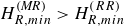 $H_{R,min }^{(\textit{MR})}\gt H_{R,min }^{(RR)}$
, assumed by Li & Ben-Dor (Reference Li and Ben-Dor1997) without proof, holds in a large part of the dual-solution domain. This would have not been possible since
$H_{R,min }^{(\textit{MR})}\gt H_{R,min }^{(RR)}$
, assumed by Li & Ben-Dor (Reference Li and Ben-Dor1997) without proof, holds in a large part of the dual-solution domain. This would have not been possible since $H_{R,min }^{(\textit{MR})}$
depends on the Mach stem height. To overcome this difficulty, we have used proof by transitivity, through finding a lower bound of
$H_{R,min }^{(\textit{MR})}$
depends on the Mach stem height. To overcome this difficulty, we have used proof by transitivity, through finding a lower bound of $H_{R,min }^{(\textit{MR})}$
that corresponds to the minimum Mach stem height. We have shown that
$H_{R,min }^{(\textit{MR})}$
that corresponds to the minimum Mach stem height. We have shown that $H_{R,min }^{(\textit{MR})}\gt H_{R,min }^{(RR)}$
holds within the dual-solution domain, sufficiently far away from the tip horn corner of the dual-solution domain. The proof of the inequality means that there indeed exists a dual-solution stability gap for
$H_{R,min }^{(\textit{MR})}\gt H_{R,min }^{(RR)}$
holds within the dual-solution domain, sufficiently far away from the tip horn corner of the dual-solution domain. The proof of the inequality means that there indeed exists a dual-solution stability gap for $H_{R}$
between the lower limit
$H_{R}$
between the lower limit $H_{R,min }^{(RR)}$
(called the subcritical threshold) and the lower limit
$H_{R,min }^{(RR)}$
(called the subcritical threshold) and the lower limit $H_{R,min }^{(\textit{MR})}$
(called the supercritical threshold). Above the supercritical threshold, both RR and MR can be stable, i.e. we may have steady stable RR and MR solutions in the dual-solution domain. Below the subcritical threshold, both RR and MR are unstable. Between the subcritical threshold and the supercritical threshold; RR is stable and MR is unstable.
$H_{R,min }^{(\textit{MR})}$
(called the supercritical threshold). Above the supercritical threshold, both RR and MR can be stable, i.e. we may have steady stable RR and MR solutions in the dual-solution domain. Below the subcritical threshold, both RR and MR are unstable. Between the subcritical threshold and the supercritical threshold; RR is stable and MR is unstable.
A road map is given to obtain the accurate value of the quantity of the dual-solution stability gap. This roadmap combines the theory and numerical simulation. For three cases, we have shown that the dual-solution stability gap is large compared with the subcritical geometric threshold $H_{R,min }^{(RR)}$
. The accuracy of the roadmap is further confirmed by numerical simulation.
$H_{R,min }^{(RR)}$
. The accuracy of the roadmap is further confirmed by numerical simulation.
The confirmation of the dual-solution stability gap implies a new transition possibility: within the dual-solution stability gap, i.e. for $H_{R,min }^{(RR)}\lt H_{R}\lt H_{R,min }^{(\textit{MR})}$
, a stable RR can transit dynamically to unstable MR under suitable local disturbance. Previous studies about dynamic transition (cf. Kudyavtev et al. Reference Kudryavtsev, Khotyanovsky, Ivanov and Vandromme2002; Mouton & Hornung Reference Mouton and Hornung2007; Li et al. Reference Li, Gao and Wu2011) assumed implicitly
$H_{R,min }^{(RR)}\lt H_{R}\lt H_{R,min }^{(\textit{MR})}$
, a stable RR can transit dynamically to unstable MR under suitable local disturbance. Previous studies about dynamic transition (cf. Kudyavtev et al. Reference Kudryavtsev, Khotyanovsky, Ivanov and Vandromme2002; Mouton & Hornung Reference Mouton and Hornung2007; Li et al. Reference Li, Gao and Wu2011) assumed implicitly $H_{R}\gt H_{R,min }^{(\textit{MR})}$
, so dynamic transition leads to stable MR. Here, we indeed observe dynamic transition from stable RR to unstable MR, through numerical simulation with density perturbation, for the particular condition with
$H_{R}\gt H_{R,min }^{(\textit{MR})}$
, so dynamic transition leads to stable MR. Here, we indeed observe dynamic transition from stable RR to unstable MR, through numerical simulation with density perturbation, for the particular condition with $M_{0}=4$
,
$M_{0}=4$
, $\theta _{w}=25^{o}$
and
$\theta _{w}=25^{o}$
and $H_{R}=0.328H_{A}$
.
$H_{R}=0.328H_{A}$
.
Numerical simulation shows various types of dynamic transition and displays various complex shock interaction structures during dynamic transition within the dual-solution stability gap. One type is direct dynamic transition for which the transition goes from RR to MR to unstart flow. The other type is inverted dynamic transition, for which RR transits to MR but then transits back to RR. Complex flow structures, such as hybrid MR –type VI shock interference, and double MR–MR, are found to exist during the dynamic transition, depending on how we provide the disturbance.
Although Vuillon et al. (Reference Vuillon, Zeitoun and Ben-Dor1995) suggested using the Mach stem height model of Azevedo & Liu (Reference Azevedo and Liu1993) to estimate the Mach stem height involved in the expression for the lower limit, the present study has avoided the use of approximate models since we need accurate values for the dual-solution stability gap. As shown by an example in Appendix A, using an approximate model to evaluate $A$
and
$A$
and $B$
and then using them in expressions (3.9) and (3.10) (§ 3) for the dual-solution stability gap may lead to significant errors.
$B$
and then using them in expressions (3.9) and (3.10) (§ 3) for the dual-solution stability gap may lead to significant errors.
The present study has focused on inviscid two-dimensional flow. In real flow, the wedge low surface has a boundary layer, which alters the effective wedge angle and the effective trailing-edge height (see Appendix B for a short discussion about how to make a simple correction accounting for the boundary-layer effect). Three-dimensional effects may also alter the stability gap. Threadgill & Little (Reference Threadgill and Little2020) have shown that the swept angle of the leading edge affects shock reflections, by reducing the effective Mach number and altering the effective wedge angle. Thus, the swept angle effect may be accounted for through replacing the Mach number and wedge angle by their effective ones.
Acknowledgements
The authors thank the referees for their valuable comments leading to improvement of this manuscript.
Funding
This work was supported partly by the National Key Project (Grant no. GJXM92579) and by the National Science and Technology Major Project 2017-II-003-0015.
Declaration of interests
The authors report no conflict of interest.
Appendix A. Limitation of approximate modelling
This appendix is to report the stability gap when the coefficients $A$
and
$A$
and $B$
required in expression (3.9) (§ 3) are given by an approximate Mach stem height. The purpose here is to how the results based on simplified modelling may be not accurate compared with the results obtained from the roadmap proposed in § 3. Since the work of Azevedo (Reference Azevedo1989) (see also Azevedo & Liu Reference Azevedo and Liu1993), several Mach stem height models have been proposed (e.g. Li & BenDor Reference Li and Ben-Dor1997; Mouton & Hornung Reference Mouton and Hornung2007; Gao & Wu Reference Gao and Wu2010; Bai & Wu Reference Bai and Wu2017; Bai & Wu Reference Bai and Wu2021).
$B$
required in expression (3.9) (§ 3) are given by an approximate Mach stem height. The purpose here is to how the results based on simplified modelling may be not accurate compared with the results obtained from the roadmap proposed in § 3. Since the work of Azevedo (Reference Azevedo1989) (see also Azevedo & Liu Reference Azevedo and Liu1993), several Mach stem height models have been proposed (e.g. Li & BenDor Reference Li and Ben-Dor1997; Mouton & Hornung Reference Mouton and Hornung2007; Gao & Wu Reference Gao and Wu2010; Bai & Wu Reference Bai and Wu2017; Bai & Wu Reference Bai and Wu2021).
Now we try the approximate model of Bai & Wu (Reference Bai and Wu2021, equation (25)) for $A$
and
$A$
and $B$
to compute
$B$
to compute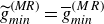 $\widetilde {g}_{\textit{min}}^{(\textit{MR})}=\overline {g}_{\textit{min}}^{{\small (MR)}}$
by (3.9).
$\widetilde {g}_{\textit{min}}^{(\textit{MR})}=\overline {g}_{\textit{min}}^{{\small (MR)}}$
by (3.9).
The resulting value of $\triangle \widetilde {g}_{\textit{min}}=\widetilde {g}_{\textit{min}}^{(\textit{MR})}-g_{\textit{min}}^{(RR)}$
by (3.10) is displayed in figure 13. For comparison we consider the three cases shown in table 2.
$\triangle \widetilde {g}_{\textit{min}}=\widetilde {g}_{\textit{min}}^{(\textit{MR})}-g_{\textit{min}}^{(RR)}$
by (3.10) is displayed in figure 13. For comparison we consider the three cases shown in table 2.
Contourlines of $\triangle \widetilde {g}_{\textit{min}}$
give the approximate method; (a) global view, (b) enlarged view.
$\triangle \widetilde {g}_{\textit{min}}$
give the approximate method; (a) global view, (b) enlarged view.

For case 1, we have $\triangle \overline {g}_{\textit{min}}=0.178$
according to table 2, while by figure 13,
$\triangle \overline {g}_{\textit{min}}=0.178$
according to table 2, while by figure 13, $\triangle \widetilde {g}_{\textit{min}}\approx 0.12$
. Thus, the difference between
$\triangle \widetilde {g}_{\textit{min}}\approx 0.12$
. Thus, the difference between $\triangle \overline {g}_{\textit{min}}$
and
$\triangle \overline {g}_{\textit{min}}$
and $\triangle \widetilde {g}_{\textit{min}}$
is as large as
$\triangle \widetilde {g}_{\textit{min}}$
is as large as $33\,\%$
. This means that, for case 1, the approximate method underestimates the dual-solution stability gap by
$33\,\%$
. This means that, for case 1, the approximate method underestimates the dual-solution stability gap by $33\,\%$
.
$33\,\%$
.
Now consider case 2. We have $\triangle \overline {g}_{\textit{min}}=0.091$
according to table 2, while by figure 13,
$\triangle \overline {g}_{\textit{min}}=0.091$
according to table 2, while by figure 13, $\triangle \widetilde {g}_{\textit{min}}\approx 0.03$
. Thus, the approximate method underestimates the dual-solution stability gap by
$\triangle \widetilde {g}_{\textit{min}}\approx 0.03$
. Thus, the approximate method underestimates the dual-solution stability gap by $67\,\%$
.
$67\,\%$
.
Last, we consider case 3. We have $\triangle \overline {g}_{\textit{min}}=0.185$
according to table 2, while by figure 13,
$\triangle \overline {g}_{\textit{min}}=0.185$
according to table 2, while by figure 13, $\triangle \widetilde {g}_{\textit{min}}\approx 0.12$
. Thus, the approximate method underestimates the dual-solution stability gap by
$\triangle \widetilde {g}_{\textit{min}}\approx 0.12$
. Thus, the approximate method underestimates the dual-solution stability gap by $35\,\%$
.
$35\,\%$
.
In conclusion, the simplified modelling used above does not yield quantitative correct estimation of the dual-solution stability gap, and this is why we proposed the roadmap presented in § 3.
Appendix B. Discussion of the effect of the boundary layer
The present study is a two-dimensional inviscid study. Practical flow has a boundary layer. For shock reflection, there are two alternative ways to account for the effect of the boundary layer.
One is to use the shock angle $\beta _{01}$
of the incident shock, as by Hornung & Robinson (Reference Hornung and Robinson1982) for experimental study and by Li & Ben-Dor (Reference Li and Ben-Dor1997) for analytical study of the Mach stem height. Practically, the shock angle depends not only on
$\beta _{01}$
of the incident shock, as by Hornung & Robinson (Reference Hornung and Robinson1982) for experimental study and by Li & Ben-Dor (Reference Li and Ben-Dor1997) for analytical study of the Mach stem height. Practically, the shock angle depends not only on $M_{0}$
and
$M_{0}$
and $\theta _{w}$
, but also on the thickness of the boundary layer, which in turn depends on the Mach number and Reynolds number. Using
$\theta _{w}$
, but also on the thickness of the boundary layer, which in turn depends on the Mach number and Reynolds number. Using $\beta _{01}$
automatically accounts for the effect of the boundary layer. To apply the present result which uses
$\beta _{01}$
automatically accounts for the effect of the boundary layer. To apply the present result which uses $\theta _{w}$
as one input parameter, we may, for each real
$\theta _{w}$
as one input parameter, we may, for each real $\beta _{01}$
(which accounts for the boundary layer in a real situation), we use the shock angle relation
$\beta _{01}$
(which accounts for the boundary layer in a real situation), we use the shock angle relation
 \begin{align} \tan \theta _{w}^{(e)}=f_{\theta }(M_{0},\beta _{01}) \end{align}
to find the equivalent wedge angle $\theta _{w}^{(e)}$
(which accounts for the effect of the boundary layer). Then, we replace
$\theta _{w}^{(e)}$
(which accounts for the effect of the boundary layer). Then, we replace $\theta _{w}$
by
$\theta _{w}$
by $\theta _{w}^{(e)}$
in the theory presented in §§ 2 and 3, to obtain the dual-solution stability gap.
$\theta _{w}^{(e)}$
in the theory presented in §§ 2 and 3, to obtain the dual-solution stability gap.
The second one is to use boundary-layer correction, by adding the displacement thickness correction to $\theta _{w}$
. Details of this method have been given by Chen et al. (Reference Chen, Bai and Wu2020), who provided an explicit method to evaluate the displacement thickness and its correction to
$\theta _{w}$
. Details of this method have been given by Chen et al. (Reference Chen, Bai and Wu2020), who provided an explicit method to evaluate the displacement thickness and its correction to $\theta _{w}$
, and showed that such a correction can effectively account for the effect of the boundary layer when compared with numerical simulation.
$\theta _{w}$
, and showed that such a correction can effectively account for the effect of the boundary layer when compared with numerical simulation.
Chen et al. (Reference Chen, Bai and Wu2020) also showed that the boundary layer gives a correction to the effective trailing-edge height ( $g^{(e)}$
), and showed that the existence of the boundary layer reduces the trailing-edge height.
$g^{(e)}$
), and showed that the existence of the boundary layer reduces the trailing-edge height.
Overall, the boundary layer increases the effective $\theta _{w}$
or the shock angle, and reduces the effective trailing-edge height
$\theta _{w}$
or the shock angle, and reduces the effective trailing-edge height $g$
. The introduction of the explicit formulas for the correction of
$g$
. The introduction of the explicit formulas for the correction of $\theta _{w}$
and of
$\theta _{w}$
and of $g$
into the formulas of §§ 2 and 3 where
$g$
into the formulas of §§ 2 and 3 where $\theta _{w}$
and
$\theta _{w}$
and $g$
are involved can yields the results when the boundary layer is considered. Thus, it is possible that the boundary-layer effects may not change the primary conclusions of this study, i.e. if the above correction is introduced so that the parameter space is replaced by the equivalent ones (
$g$
are involved can yields the results when the boundary layer is considered. Thus, it is possible that the boundary-layer effects may not change the primary conclusions of this study, i.e. if the above correction is introduced so that the parameter space is replaced by the equivalent ones ( $\theta _{w}^{(e)}$
and
$\theta _{w}^{(e)}$
and $g^{(e)}$
), the predicted critical thresholds might remain applicable, and the observed stability or instability of the MR and RR structures might remain unchanged. However, a detailed consideration of this correction merits a study in the future.
$g^{(e)}$
), the predicted critical thresholds might remain applicable, and the observed stability or instability of the MR and RR structures might remain unchanged. However, a detailed consideration of this correction merits a study in the future.
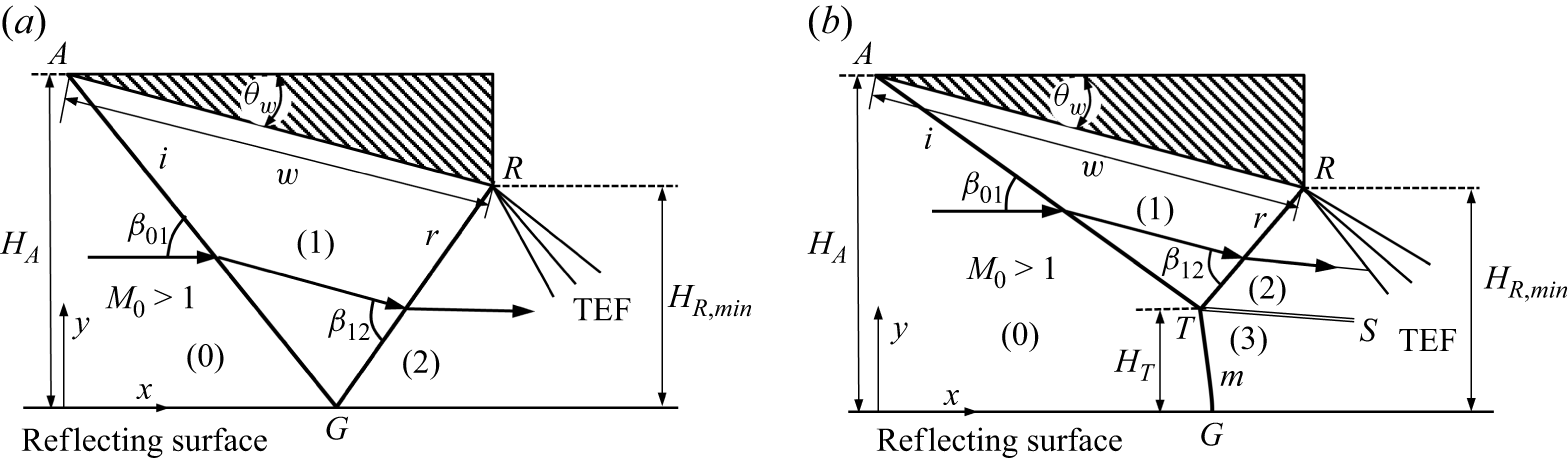


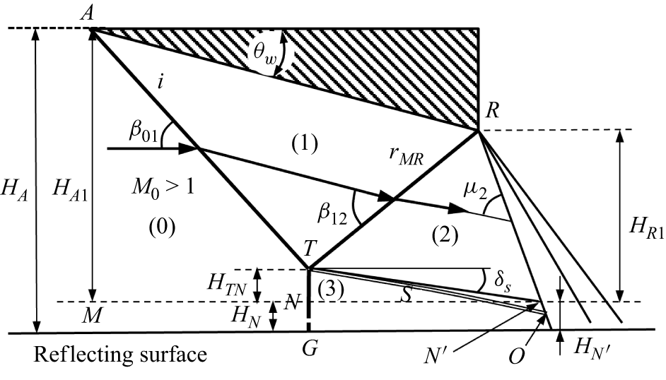


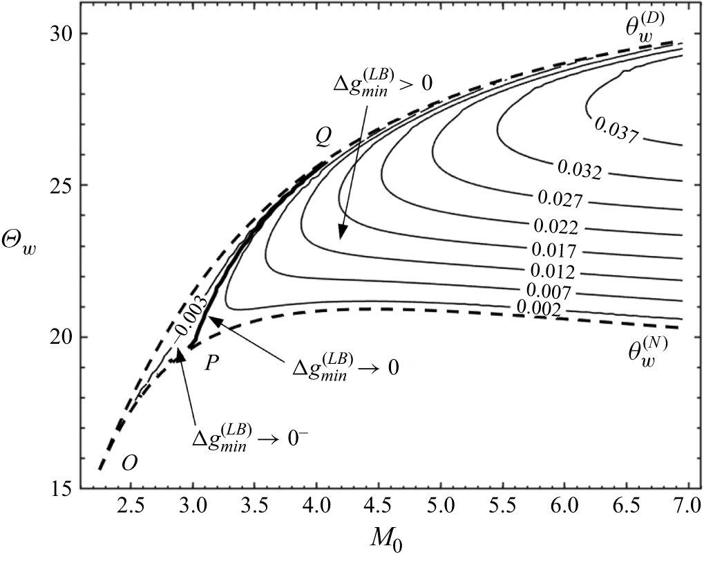


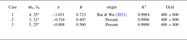


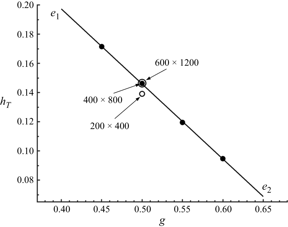


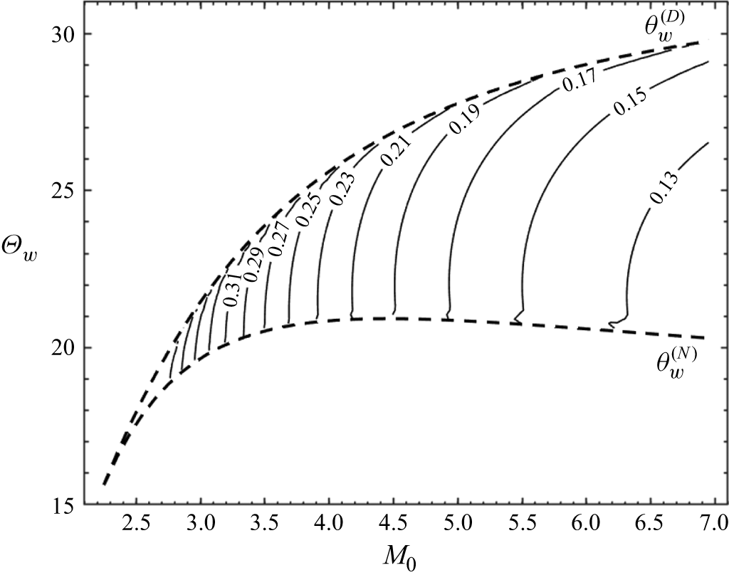

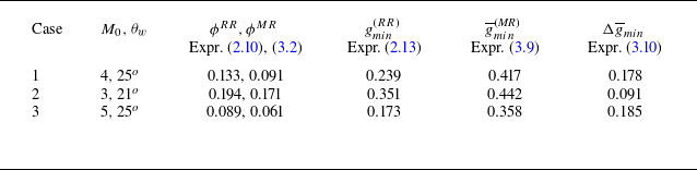


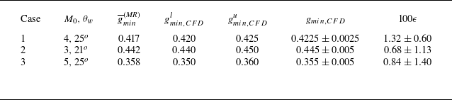


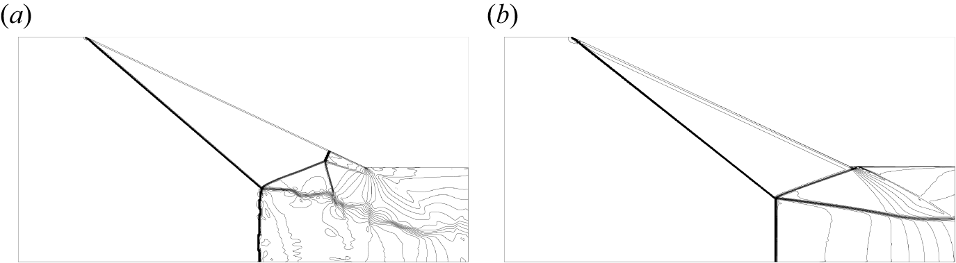


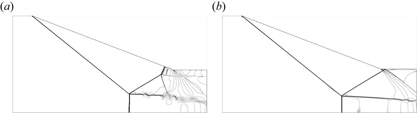


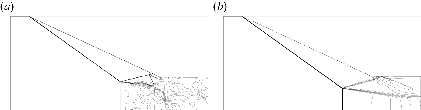


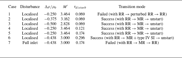


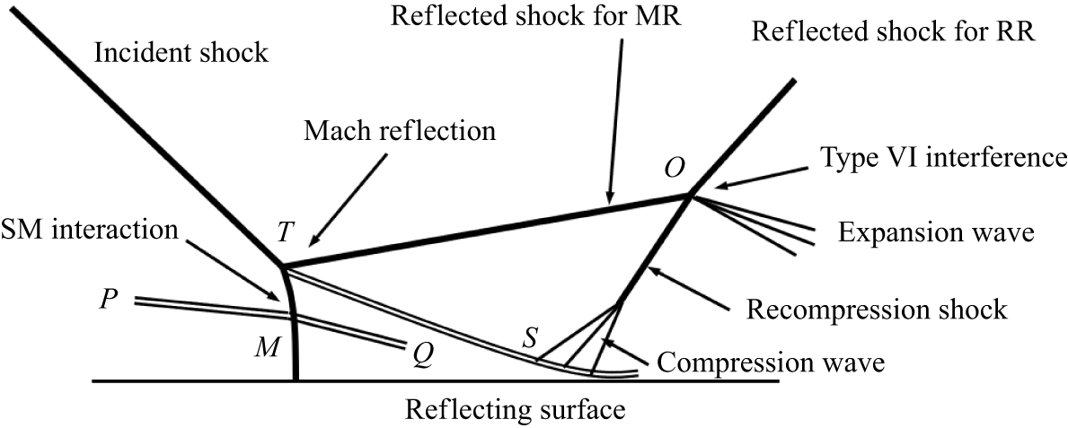

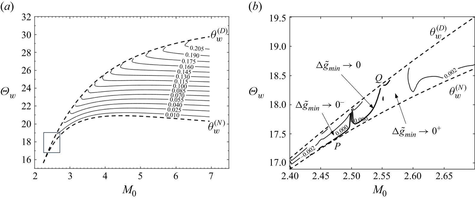


 Open access

