





1. Introduction
Secondary currents (SCs) are mean cross-stream motions with streamwise vorticity that arise in wall-bounded turbulence in the presence of spanwise inhomogeneity. Following Prandtl (Reference Prandtl1952), they are commonly classified as secondary motions of the second kind, sustained by anisotropy and spatial gradients of Reynolds stresses. Although their velocity magnitude is typically small compared with the bulk flow, SCs can exert a disproportionate influence on wall-bounded turbulence by redistributing momentum over large wall-normal distances and by imposing persistent large-scale organisation on the mean flow. In spanwise-heterogeneous configurations, this redistribution commonly produces alternating low- and high-momentum pathways (LMPs and HMPs), associated with local boundary-layer thickening and thinning. Such behaviour has been documented in wind-tunnel experiments over alternating roughness (Barros & Christensen Reference Barros and Christensen2014), in open-channel flows over sediment-induced heterogeneity (Nugroho, Hutchins & Monty Reference Nugroho, Hutchins and Monty2013) and in systematically designed roughness arrays (Kevin et al. Reference Kevin, Monty, Bai, Pathikonda, Nugroho, Barros, Christensen and Hutchins2017). As the characteristic heterogeneity scale approaches the flow depth, SCs become increasingly prominent and the assumptions of classical outer-layer similarity become progressively less reliable.
This behaviour challenges the applicability of Townsend’s outer-layer similarity hypothesis (Townsend Reference Townsend1976), which assumes that turbulence in the outer region becomes independent of wall conditions at sufficiently high Reynolds numbers. As noted by Jiménez (Reference Jiménez2004), however, this assumption requires a clear scale separation between the roughness height and the outer flow thickness, a condition that is often not satisfied when roughness-induced SCs extend well into the outer layer. Under such circumstances, the turbulence remains sensitive to the wall condition over a broad wall-normal range. This sensitivity has direct dynamical consequences, including drag levels exceeding the area-weighted expectation of the underlying surface types (Stroh et al. Reference Stroh, Schäfer, Frohnapfel and Forooghi2020), as well as substantial spanwise asymmetries in momentum and energy transport. In such flows, the effect of roughness heterogeneity is therefore not limited to modifying local turbulence intensity; rather, it reorganises the mean flow and introduces form-induced transport pathways that must be treated explicitly within a double-averaging framework (Raupach & Shaw Reference Raupach and Shaw1982; Nikora et al. Reference Nikora, McEwan, McLean, Coleman, Pokrajac and Walters2007).
The structure and strength of SCs depend strongly on how the spanwise heterogeneity is imposed. In strip-type configurations, neighbouring wall regions impose different shear stresses, giving rise to lateral gradients in turbulence production and counter-rotating secondary motions, typically with upwelling above low-shear zones and downwelling above high-shear zones (Hinze Reference Hinze1973; Willingham et al. Reference Willingham, Anderson, Christensen and Barros2014; Anderson et al. Reference Anderson, Barros, Christensen and Awasthi2015; Chung, Monty & Hutchins Reference Chung, Monty and Hutchins2018). In ridge-type heterogeneity, elevation differences similarly induce large-scale circulations, commonly with upward motion over elevated regions and downward motion over depressed regions, although the detailed structure depends on the ridge morphology and spacing (Nezu & Nakagawa Reference Nezu and Nakagawa1984; Goldstein & Tuan Reference Goldstein and Tuan1998; Wang & Cheng Reference Wang and Cheng2006; Vanderwel & Ganapathisubramani Reference Vanderwel and Ganapathisubramani2015; Hwang & Lee Reference Hwang and Lee2018; Medjnoun, Vanderwel & Ganapathisubramani Reference Medjnoun, Vanderwel and Ganapathisubramani2018). In realistic rough-wall flows, however, wall-shear variation and geometric roughness often coexist, and the resulting SCs cannot be interpreted as a purely strip-type or purely ridge-type response. The present study therefore considers roughness strips composed of fixed spherical elements, which provide a three-dimensional spanwise-heterogeneous configuration combining geometric elevation effects and roughness-induced drag variation in a form more representative of practical rough-wall open-channel flows.
In parallel with these developments, the dynamics of very-large-scale motions (VLSMs) in canonical wall turbulence have been widely documented. In smooth-wall boundary layers, channels and pipes, VLSMs are among the most energetic and coherent outer-layer structures, with streamwise extents far exceeding those of large-scale motions (LSMs) (Kim & Adrian Reference Kim and Adrian1999; Guala, Hommema & Ddrian Reference Guala, Hommema and Ddrian2006; Balakumar & Adrian Reference Balakumar and Adrian2007; Monty et al. Reference Monty, Stewart, Williams and Chong2007; Wu, Baltzer & Adrian Reference Wu, Baltzer and Adrian2012; Ahn et al. Reference Ahn, Lee, Lee, Kang and Sung2015). Their dynamical importance lies not only in their energetic dominance in the outer layer, but also in their footprint on the near-wall region through inner–outer coupling, amplitude modulation and scale interaction (Hutchins & Marusic Reference Hutchins and Marusic2007a , Reference Hutchins and Marusicb ; Mathis, Hutchins & Marusic Reference Mathis, Hutchins and Marusic2009; Ganapathisubramani et al. Reference Ganapathisubramani, Hutchins, Monty, Chung and Marusic2012). For open-channel flows, the existence of VLSMs has also been established over rough beds, where they contribute to the large-scale turbulent organisation of the flow (Cameron, Nikora & Stewart Reference Cameron, Nikora and Stewart2017). These studies collectively show that VLSMs are not merely spectral features, but key carriers of momentum and energy across the outer region of wall-bounded turbulence.
Over spanwise-heterogeneous roughness, however, the relationship between SCs and VLSMs becomes considerably more complex. Increasing evidence suggests that SCs can disrupt the canonical outer-layer organisation and impose an alternative large-scale structure that is locked to the surface heterogeneity. Awasthi & Anderson (Reference Awasthi and Anderson2018) showed that, over spanwise-topographically heterogeneous surfaces, the spectral signature of large-scale motions is retained in some regions, but strongly attenuated in others, indicating a spatially selective modulation by SCs. Yang & Anderson (Reference Yang and Anderson2018) further demonstrated that topographic heterogeneity alters the outer-layer turbulence structure and weakens the canonical large-scale signature. In open-channel flow over streamwise ridges, Zampiron, Cameron & Nikora (Reference Zampiron, Cameron and Nikora2020) showed that strong SCs coexist with, and can substantially modify, VLSM activity. More recently, Wangsawijaya & Hutchins (Reference Wangsawijaya and Hutchins2022) revisited heterogeneous turbulent boundary layers and emphasised the coupled role of unsteady secondary motions and large-scale turbulence organisation, further underscoring that SCs and large-scale motions should not be studied in isolation.
At the same time, recent work has begun to show that the roughness effect on large-scale turbulence is not exhausted by changes in spectral energy alone. Instead, roughness-induced heterogeneity can reorganise the pathways through which momentum and energy are redistributed across scales. In rough-wall channel flow with randomly distributed roughness, Ma et al. (Reference Ma, Xu, Sung, Tian and Huang2025) demonstrated that form-induced structures play an essential role in inter-scale energy transfer. In open-channel flow over streamwise ridges, Zampiron, Cameron & Nikora (Reference Zampiron, Cameron and Nikora2021) showed that the double-averaged momentum and energy budgets are strongly shaped by ridge-induced SCs, highlighting the importance of separating turbulent transport from form-induced transport. These developments suggest that the relevant question is not simply whether SCs suppress or amplify VLSMs, but how roughness-induced SCs reorganise the large-scale flow, alter the balance between turbulent and form-induced transport, and modify the scale-dependent pathway by which energy is redistributed from outer large-scale motions towards near-wall turbulence.
Despite these advances, a unified physical picture linking roughness-induced SCs, form-induced transport, VLSM organisation and scale-dependent energy redistribution remains lacking, particularly for open-channel flows over spanwise-heterogeneous roughness composed of discrete three-dimensional elements. In particular, it remains unclear how the geometry-locked SCs generated by such roughness first reorganise the mean momentum field and form-induced stresses, then alter the occurrence and spatial distribution of positive- and negative-velocity VLSMs, and finally reshape the inter-scale energy pathway associated with large-scale motions. Clarifying this chain is essential if one is to move beyond the simplified picture of VLSMs being merely weakened or strengthened by roughness, and instead understand how roughness heterogeneity redirects the multi-scale dynamics of wall-bounded turbulence.
Motivated by this gap, the present study investigates turbulent open-channel flow over spanwise-heterogeneous roughness strips composed of fixed spherical elements. The central objective is to clarify how roughness-induced SCs mediate the connection between mean-flow reorganisation, form-induced transport, VLSM organisation and inter-scale energy transfer. The analysis shows that the dominant role of the roughness strips is not a uniform amplification of turbulence intensity, but the generation of persistent, geometry-locked SCs that organise the mean flow into HMPs and LMPs, and strongly enhance form-induced stresses. Within this reorganised flow field, VLSMs are not simply suppressed or intensified uniformly; instead, they undergo a sign-dependent and roughness-conditioned reorganisation. Spectral and triadic analyses further reveal that this kinematic reorganisation is accompanied by a scale-dependent energy-redistribution pathway involving an outer-scale organisational footprint and a smaller near-wall active scale.
The remainder of the paper is organised as follows. Section 2 describes the governing equations, numerical methodology, simulation set-up and validation procedure. Section 3 presents the effects of spanwise-heterogeneous roughness on the double-averaged stresses, the structure of roughness-induced SCs, the sign-dependent reorganisation of VLSMs and the associated inter-scale energy-redistribution pathways. Finally, § 4 summarises the main conclusions, and discusses the scope and limitations of the present simulations.
2. Methodology and validation
2.1. Mathematical formulation and simulation set-up
The present study considers a fully developed three-dimensional open-channel turbulent flow over spanwise-non-uniform roughness strips, as illustrated in figure 1(c). Five laterally aligned roughness strips, each composed of fixed spherical roughness elements, are installed on the channel bed to introduce spanwise geometric heterogeneity and thereby promote SCs. The geometric configuration of the roughness strips is shown in figures 1(a) and 1(b), where $D$
denotes the diameter of the spherical roughness elements – numerically equivalent to the strip height
$D$
denotes the diameter of the spherical roughness elements – numerically equivalent to the strip height $y_0$
– and
$y_0$
– and $S$
is the spanwise spacing between adjacent strips. Following the experimental findings of Wangsawijaya et al. (Reference Wangsawijaya, Baidya, Chung, Marusic and Hutchins2020), the intensity of secondary motions is maximised when the strip spacing is comparable to the channel height
$S$
is the spanwise spacing between adjacent strips. Following the experimental findings of Wangsawijaya et al. (Reference Wangsawijaya, Baidya, Chung, Marusic and Hutchins2020), the intensity of secondary motions is maximised when the strip spacing is comparable to the channel height $h$
. Motivated by this observation, the present study sets
$h$
. Motivated by this observation, the present study sets $S=1.2h$
to further examine how roughness strips composed of spherical elements at different elevations influence the resultant secondary flow and turbulence dynamics.
$S=1.2h$
to further examine how roughness strips composed of spherical elements at different elevations influence the resultant secondary flow and turbulence dynamics.
Computational domain and roughness configuration. Panels (a, b) show schematic layouts of the spherical roughness strips with streamwise- and spanwise-heterogeneous arrangements, where $D$
is the sphere diameter (equal to the strip height
$D$
is the sphere diameter (equal to the strip height $y_0$
) and
$y_0$
) and $S$
is the spanwise spacing. Panel (c) presents the three-dimensional open-channel domain with five laterally aligned roughness strips; the spacing is set to
$S$
is the spanwise spacing. Panel (c) presents the three-dimensional open-channel domain with five laterally aligned roughness strips; the spacing is set to $S = 1.2h$
.
$S = 1.2h$
.

The incompressible Navier–Stokes equations are solved in their velocity–pressure form using a fractional-step projection method,
 \begin{equation} \frac {\partial u_i}{\partial t} + u_{\!j} \frac {\partial u_i}{\partial x_j} = - \frac {\partial p}{\partial x_i} + \nu \frac {\partial ^2 u_i}{\partial x_j^2} + f_i^{\textit{IBM}}, \end{equation}
subject to the incompressibility constraint
 \begin{equation} \frac {\partial u_i}{\partial x_i} = 0 . \end{equation}
Here, $u_i=(u,v,w)$
are the velocity components in the Cartesian directions
$u_i=(u,v,w)$
are the velocity components in the Cartesian directions $x_i=(x,y,z)$
,
$x_i=(x,y,z)$
, $p$
is the pressure,
$p$
is the pressure, $\nu$
is the kinematic viscosity and
$\nu$
is the kinematic viscosity and $f_i^{\textit{IBM}}$
denotes the immersed-boundary forcing used to impose the no-slip condition on the spherical roughness elements. The nonlinear convective terms are advanced explicitly with a second-order Adams–Bashforth scheme, while viscous diffusion is treated explicitly. The pressure Poisson equation is solved at the end of each time step to enforce the divergence-free condition. Spatial discretisation employs Fourier expansions in the streamwise and spanwise directions, both of which are strictly periodic, whereas the wall-normal direction is discretised using second-order finite differences on a non-stretched grid. The bottom wall is no-slip, while the top boundary is treated as free-slip, consistent with the configuration of an open-channel flow. The interaction between the fluid and the fixed spherical roughness elements is handled using a direct-forcing immersed-boundary method following Kempe & Fröhlich (Reference Kempe and Fröhlich2012). At each Adams–Bashforth stage, a Lagrangian forcing term is computed to impose the no-slip condition on the particle surfaces by driving the local fluid velocity towards the prescribed solid velocity (zero for the stationary spheres). This force is then projected onto the Eulerian mesh using an
$f_i^{\textit{IBM}}$
denotes the immersed-boundary forcing used to impose the no-slip condition on the spherical roughness elements. The nonlinear convective terms are advanced explicitly with a second-order Adams–Bashforth scheme, while viscous diffusion is treated explicitly. The pressure Poisson equation is solved at the end of each time step to enforce the divergence-free condition. Spatial discretisation employs Fourier expansions in the streamwise and spanwise directions, both of which are strictly periodic, whereas the wall-normal direction is discretised using second-order finite differences on a non-stretched grid. The bottom wall is no-slip, while the top boundary is treated as free-slip, consistent with the configuration of an open-channel flow. The interaction between the fluid and the fixed spherical roughness elements is handled using a direct-forcing immersed-boundary method following Kempe & Fröhlich (Reference Kempe and Fröhlich2012). At each Adams–Bashforth stage, a Lagrangian forcing term is computed to impose the no-slip condition on the particle surfaces by driving the local fluid velocity towards the prescribed solid velocity (zero for the stationary spheres). This force is then projected onto the Eulerian mesh using an $800$
-point partition, ensuring smooth and conservative momentum exchange between the Lagrangian markers and the Eulerian flow field. The geometric representation of the roughness and the corresponding forcing supports are updated using the NBS–Munijiza search algorithm, which accurately identifies the fluid grid points influenced by each roughness element. As the spheres remain completely stationary, they form a laterally uniform stripwise roughness pattern that provides a fully resolved geometric boundary condition, thereby modulating near-wall turbulence and inducing large-scale organisation in the outer region of the flow.
$800$
-point partition, ensuring smooth and conservative momentum exchange between the Lagrangian markers and the Eulerian flow field. The geometric representation of the roughness and the corresponding forcing supports are updated using the NBS–Munijiza search algorithm, which accurately identifies the fluid grid points influenced by each roughness element. As the spheres remain completely stationary, they form a laterally uniform stripwise roughness pattern that provides a fully resolved geometric boundary condition, thereby modulating near-wall turbulence and inducing large-scale organisation in the outer region of the flow.
Boundary conditions are specified as follows. In the streamwise ( $x$
) and spanwise (
$x$
) and spanwise ( $z$
) directions, the flow is periodic. At the bottom boundary, a no-slip rough wall is imposed through immersed-boundary-resolved spherical roughness elements. At the top boundary, a free-slip condition is used, consistent with the open-channel configuration. A constant bulk velocity is maintained by dynamically adjusting the mean streamwise pressure gradient. The present set-up is therefore a spatially periodic DNS of statistically fully developed open-channel turbulence rather than a spatially developing inflow–outflow simulation. The free-slip top boundary provides a simplified open-channel representation without resolving free-surface deformation. The roughness elements are fixed, stationary and fully resolved spheres, with the no-slip condition on each sphere surface enforced by direct forcing.
$z$
) directions, the flow is periodic. At the bottom boundary, a no-slip rough wall is imposed through immersed-boundary-resolved spherical roughness elements. At the top boundary, a free-slip condition is used, consistent with the open-channel configuration. A constant bulk velocity is maintained by dynamically adjusting the mean streamwise pressure gradient. The present set-up is therefore a spatially periodic DNS of statistically fully developed open-channel turbulence rather than a spatially developing inflow–outflow simulation. The free-slip top boundary provides a simplified open-channel representation without resolving free-surface deformation. The roughness elements are fixed, stationary and fully resolved spheres, with the no-slip condition on each sphere surface enforced by direct forcing.
For the baseline simulations, the computational domain size is $L_x \times L_y \times L_z = 12h \times h \times 6h$
with grid resolution
$L_x \times L_y \times L_z = 12h \times h \times 6h$
with grid resolution $N_x \times N_y \times N_z = 648 \times 196 \times 576$
. The corresponding wall-unit resolutions are reported in table 1. All baseline cases are computed within the same numerical framework and the roughness effect is characterised by the mean roughness height in wall units,
$N_x \times N_y \times N_z = 648 \times 196 \times 576$
. The corresponding wall-unit resolutions are reported in table 1. All baseline cases are computed within the same numerical framework and the roughness effect is characterised by the mean roughness height in wall units,
 \begin{equation} k_a^{+} = k_a u_{\tau }/\nu . \end{equation}
Computational parameters and grid resolution in viscous units for all cases. The domain dimensions are reported as $L_x/h \times L_y/h \times L_z/h$
, while
$L_x/h \times L_y/h \times L_z/h$
, while $\Delta x^{+}$
,
$\Delta x^{+}$
, $\Delta y^{+}$
and
$\Delta y^{+}$
and $\Delta z^{+}$
denote the grid resolutions in viscous units.
$\Delta z^{+}$
denote the grid resolutions in viscous units.

Here, $k_a$
is the roughness-element height measured from the bottom wall to the roughness crest,
$k_a$
is the roughness-element height measured from the bottom wall to the roughness crest, $u_{\tau }$
is the friction velocity and
$u_{\tau }$
is the friction velocity and $\nu$
is the kinematic viscosity. In the present spherical roughness-strip configuration,
$\nu$
is the kinematic viscosity. In the present spherical roughness-strip configuration, $k_a$
corresponds to the strip height. As summarised in table 1,
$k_a$
corresponds to the strip height. As summarised in table 1, $k_a^{+}$
increases systematically from the smooth-wall case to R13, R17 and R20, accompanied by corresponding increases in the friction Reynolds number
$k_a^{+}$
increases systematically from the smooth-wall case to R13, R17 and R20, accompanied by corresponding increases in the friction Reynolds number ${\textit{Re}}_{\tau }$
and the skin-friction coefficient
${\textit{Re}}_{\tau }$
and the skin-friction coefficient $C_{\!f}$
.
$C_{\!f}$
.
To provide an additional reference for isolating the role of spanwise heterogeneity from that of roughness itself, an extra homogeneous roughness case, denoted as R17 homogeneous, is introduced. In this case, roughness elements identical in size to those of R17 are distributed over the entire bottom surface, so that the wall is roughened homogeneously without spanwise stripwise alternation. The computational domain and grid resolution remain the same as those of the baseline cases. The numerical method, boundary conditions and statistical procedures are also unchanged. The corresponding parameters of this reference case are included in table 1. In addition, its mean-velocity downward shift is quantified by the roughness function, for which the present calculation gives $\Delta U^{+}=5.69$
. The comparison of the mean velocity profiles among the smooth-wall case, R17 and R17 homogeneous is shown in figure 2, which helps distinguish the effect of homogeneous roughness from the additional modulation introduced by spanwise heterogeneity.
$\Delta U^{+}=5.69$
. The comparison of the mean velocity profiles among the smooth-wall case, R17 and R17 homogeneous is shown in figure 2, which helps distinguish the effect of homogeneous roughness from the additional modulation introduced by spanwise heterogeneity.
Mean velocity profiles in inner scaling for the smooth-wall case, the spanwise-heterogeneous roughness cases and the additional homogeneous roughness reference case R17 homogeneous.

To assess streamwise-domain sensitivity, we additionally consider an extended-domain validation case with $L_x=24h$
. The streamwise grid is increased correspondingly to
$L_x=24h$
. The streamwise grid is increased correspondingly to $N_x=1296$
so that the streamwise grid spacing remains unchanged. The roughness configuration, numerical method and all boundary conditions are otherwise identical to the baseline set-up. In particular, the extended-domain case retains the same periodicity in
$N_x=1296$
so that the streamwise grid spacing remains unchanged. The roughness configuration, numerical method and all boundary conditions are otherwise identical to the baseline set-up. In particular, the extended-domain case retains the same periodicity in $x$
and
$x$
and $z$
, the same no-slip rough bottom boundary, and the same free-slip top boundary. The corresponding validation results for this extended-domain case are presented in Appendix A. In addition, to assess whether the geometry-locked secondary currents persist when the Reynolds number is reduced and the scale separation is further limited, an additional low-Reynolds-number R17 case was performed at
$z$
, the same no-slip rough bottom boundary, and the same free-slip top boundary. The corresponding validation results for this extended-domain case are presented in Appendix A. In addition, to assess whether the geometry-locked secondary currents persist when the Reynolds number is reduced and the scale separation is further limited, an additional low-Reynolds-number R17 case was performed at ${\textit{Re}}_{\tau }\approx 300$
. In this case, the roughness geometry, strip spacing, computational domain and numerical method are kept the same as in the baseline R17 case. The corresponding results are presented in Appendix B.
${\textit{Re}}_{\tau }\approx 300$
. In this case, the roughness geometry, strip spacing, computational domain and numerical method are kept the same as in the baseline R17 case. The corresponding results are presented in Appendix B.
Unless otherwise specified, statistics are accumulated over 800 saved temporal frames over a sufficiently long averaging interval to ensure statistical convergence. The numerical model does not include inflow–outflow treatment, moving or deforming roughness or resolved free-surface deformation.
2.2. Validation
For assessing the numerical reliability of the present solver in rough-bed open-channel turbulence, an additional validation case was carried out by reproducing the canonical F50 configuration of Chan-Braun, García-Villalba & Uhlmann (Reference Chan-Braun, García-Villalba and Uhlmann2011). This benchmark was chosen because it represents an immersed-boundary simulation of open-channel flow over a geometrically rough wall formed by fixed spheres, and it provides well-documented first- and second-order turbulence statistics above a rough bed. In particular, the F50 case is well suited to the present study because it directly examines the solver’s ability to predict the mean velocity profile, turbulence intensities and Reynolds shear stress in a wall-bounded rough-flow configuration, which are the key statistics required for establishing confidence in the subsequent rough-wall simulations.
In the reference study of Chan-Braun et al. (Reference Chan-Braun, García-Villalba and Uhlmann2011), the F50 configuration consists of an open-channel flow over a square arrangement of fixed spheres, with periodic boundary conditions in the streamwise and spanwise directions, a free-slip condition at the top boundary, and a no-slip condition at the bottom boundary. The computational domain is $L_x/H \times L_y/H \times L_z/H = 12 \times 1 \times 3$
, and the benchmark parameters are
$L_x/H \times L_y/H \times L_z/H = 12 \times 1 \times 3$
, and the benchmark parameters are ${\textit{Re}}_b = 2880$
,
${\textit{Re}}_b = 2880$
, ${\textit{Re}}_{\tau } = 235$
and
${\textit{Re}}_{\tau } = 235$
and $D^+ = 49.3$
. In addition, the sphere size corresponds to
$D^+ = 49.3$
. In addition, the sphere size corresponds to $H/D = 5.6$
, i.e.
$H/D = 5.6$
, i.e. $D/H = 0.179$
, which indicates that the roughness elements are of finite size relative to the flow depth. The virtual wall location is defined as
$D/H = 0.179$
, which indicates that the roughness elements are of finite size relative to the flow depth. The virtual wall location is defined as $y_0 = 0.8D$
and the friction velocity is obtained by extrapolating the linear total-shear-stress profile above the roughness layer to
$y_0 = 0.8D$
and the friction velocity is obtained by extrapolating the linear total-shear-stress profile above the roughness layer to $y = y_0$
. The flow was computed in an open-channel configuration with periodic boundary conditions in the streamwise and spanwise directions, no-slip at the rough bed, and free-slip at the top boundary, consistent with the original benchmark definition. The rough bed was represented by a fixed-sphere geometry corresponding to the F50 arrangement, containing 1024 spheres in the primary roughness layer. The computational domain and roughness geometry were constructed to preserve the same geometric proportions as the benchmark case, and the flow was discretised on a
$y = y_0$
. The flow was computed in an open-channel configuration with periodic boundary conditions in the streamwise and spanwise directions, no-slip at the rough bed, and free-slip at the top boundary, consistent with the original benchmark definition. The rough bed was represented by a fixed-sphere geometry corresponding to the F50 arrangement, containing 1024 spheres in the primary roughness layer. The computational domain and roughness geometry were constructed to preserve the same geometric proportions as the benchmark case, and the flow was discretised on a $1536 \times 128 \times 384$
Cartesian grid under a constant-bulk-flow-rate condition. Compared with the original benchmark, the present reproduction retains the same flow configuration, boundary-condition framework and roughness arrangement, while employing a reduced grid resolution.
$1536 \times 128 \times 384$
Cartesian grid under a constant-bulk-flow-rate condition. Compared with the original benchmark, the present reproduction retains the same flow configuration, boundary-condition framework and roughness arrangement, while employing a reduced grid resolution.
Following the notation of Chan-Braun et al. (Reference Chan-Braun, García-Villalba and Uhlmann2011), the present statistics were accumulated over an averaging interval corresponding to ${\textit{Tu}}{bH}/H = 8.8 \times 10^2$
, where
${\textit{Tu}}{bH}/H = 8.8 \times 10^2$
, where $u_{bH}$
denotes the bulk velocity based on the full channel height
$u_{bH}$
denotes the bulk velocity based on the full channel height $H$
. For comparison, Chan-Braun et al. (Reference Chan-Braun, García-Villalba and Uhlmann2011) reported
$H$
. For comparison, Chan-Braun et al. (Reference Chan-Braun, García-Villalba and Uhlmann2011) reported ${\textit{Tu}}{bH}/H = 120$
. The present sampling interval is therefore substantially longer than that used in the benchmark and may be regarded as sufficient, in terms of averaging duration, for the mean and second-order statistics considered here, provided that the averaging was initiated after the flow had reached a statistically stationary state.
${\textit{Tu}}{bH}/H = 120$
. The present sampling interval is therefore substantially longer than that used in the benchmark and may be regarded as sufficient, in terms of averaging duration, for the mean and second-order statistics considered here, provided that the averaging was initiated after the flow had reached a statistically stationary state.
Comparison of the reproduced F50 mean streamwise velocity profiles with the benchmark data of Chan-Braun et al. (Reference Chan-Braun, García-Villalba and Uhlmann2011): (a) $\langle u \rangle /U_{bh}$
versus
$\langle u \rangle /U_{bh}$
versus $(y-y_0)/h$
; (b)
$(y-y_0)/h$
; (b) $\langle u \rangle ^{+}$
versus
$\langle u \rangle ^{+}$
versus $(y-y_0)^{+}$
. Here,
$(y-y_0)^{+}$
. Here, $H$
is the full flow depth,
$H$
is the full flow depth, $y_0$
is the virtual wall location,
$y_0$
is the virtual wall location, $h = H-y_0$
is the effective flow depth measured from the virtual wall to the free surface,
$h = H-y_0$
is the effective flow depth measured from the virtual wall to the free surface, $U_{bh}$
is the bulk velocity defined over the effective depth
$U_{bh}$
is the bulk velocity defined over the effective depth $h$
and
$h$
and $\delta _{\nu }=\nu /u_{\tau }$
is the viscous length scale. Open circles denote the reference data and solid lines the present results. The dashed line in panel (a) marks the top of the spherical roughness elements, while the dashed line in panel (b) indicates the corresponding roughness-crest position in inner scaling.
$\delta _{\nu }=\nu /u_{\tau }$
is the viscous length scale. Open circles denote the reference data and solid lines the present results. The dashed line in panel (a) marks the top of the spherical roughness elements, while the dashed line in panel (b) indicates the corresponding roughness-crest position in inner scaling.

For validation, we reproduced the statistical quantities corresponding to the benchmark results reported by Chan-Braun et al. (Reference Chan-Braun, García-Villalba and Uhlmann2011), with particular emphasis on the mean streamwise velocity profiles in both outer and inner scalings, as presented in figure 3, together with the turbulence statistics shown in figure 4, namely the root-mean-square streamwise velocity fluctuation and the Reynolds shear stress. In figure 3(a), the mean velocity is normalised by $U_{bh}$
, the bulk velocity defined over the effective flow depth
$U_{bh}$
, the bulk velocity defined over the effective flow depth $h=H-y_0$
. Accordingly, the wall-normal coordinate is expressed as
$h=H-y_0$
. Accordingly, the wall-normal coordinate is expressed as $(y-y_0)/h$
. In figure 3(b), the mean velocity is represented in inner scaling as
$(y-y_0)/h$
. In figure 3(b), the mean velocity is represented in inner scaling as $\langle u \rangle ^{+} = \langle u \rangle /u_{\tau }$
and the wall-normal coordinate is given by
$\langle u \rangle ^{+} = \langle u \rangle /u_{\tau }$
and the wall-normal coordinate is given by $(y-y_0)^{+} = (y-y_0)u_{\tau }/\nu$
, where
$(y-y_0)^{+} = (y-y_0)u_{\tau }/\nu$
, where $u_{\tau }$
is the friction velocity and
$u_{\tau }$
is the friction velocity and $\nu$
is the kinematic viscosity. These quantities were selected because they provide a stringent and complementary assessment of the solver performance: the mean velocity profiles test the prediction of the mean momentum distribution and the roughness-induced shift of the wall-bounded flow, whereas the second-order statistics assess the ability of the numerical framework to capture the near-wall turbulent transport. In accordance with the definitions adopted by Chan-Braun et al. (Reference Chan-Braun, García-Villalba and Uhlmann2011), these statistics were obtained using whole-plane averaging over the entire streamwise–spanwise plane, including the roughness region, rather than fluid-only averaging. The friction velocity employed for inner normalisation was determined consistently with the benchmark definition, namely from the total shear-stress profile extrapolated to the virtual wall location.
$\nu$
is the kinematic viscosity. These quantities were selected because they provide a stringent and complementary assessment of the solver performance: the mean velocity profiles test the prediction of the mean momentum distribution and the roughness-induced shift of the wall-bounded flow, whereas the second-order statistics assess the ability of the numerical framework to capture the near-wall turbulent transport. In accordance with the definitions adopted by Chan-Braun et al. (Reference Chan-Braun, García-Villalba and Uhlmann2011), these statistics were obtained using whole-plane averaging over the entire streamwise–spanwise plane, including the roughness region, rather than fluid-only averaging. The friction velocity employed for inner normalisation was determined consistently with the benchmark definition, namely from the total shear-stress profile extrapolated to the virtual wall location.
Comparison of the reproduced F50 second-order turbulence statistics with the benchmark data of Chan-Braun et al. (Reference Chan-Braun, García-Villalba and Uhlmann2011): (a) $u_{\textit{rms}}/u_{\tau }$
,
$u_{\textit{rms}}/u_{\tau }$
, $v_{\textit{rms}}/u_{\tau }$
and
$v_{\textit{rms}}/u_{\tau }$
and $w_{\textit{rms}}/u_{\tau }$
versus
$w_{\textit{rms}}/u_{\tau }$
versus $(y-y_0)/h$
; (b)
$(y-y_0)/h$
; (b) $\langle u'v' \rangle /u_{\tau }^2$
versus
$\langle u'v' \rangle /u_{\tau }^2$
versus $(y-y_0)/h$
. Open symbols denote the reference data and solid lines the present results. The dashed horizontal line indicates the top of the spherical roughness elements.
$(y-y_0)/h$
. Open symbols denote the reference data and solid lines the present results. The dashed horizontal line indicates the top of the spherical roughness elements.

The comparison shows that the present solver reproduces the principal statistical features of the F50 benchmark with overall satisfactory agreement. In particular, the agreement in the mean velocity profiles indicates that the solver captures the roughness-modified mean-flow structure with reasonable accuracy, while the comparison of the streamwise turbulence intensity and Reynolds shear stress further supports that the essential characteristics of near-wall turbulent transport are also represented appropriately. Taken together, these results provide baseline validation evidence for the applicability of the present numerical framework to rough-surface open-channel flow and therefore lend support to its subsequent use for the spanwise-heterogeneous rough-wall configurations considered in this study.
3. Results and discussion
3.1. Roughness effect on turbulence statistics
In flows over spanwise-periodic roughness strips, the time-mean velocity field is intrinsically heterogeneous in the wall-parallel plane due to the presence of SCs, wake sheltering and pressure-drag footprints imposed by the roughness geometry. Under such conditions, a classical Reynolds decomposition is insufficient, as it does not distinguish turbulence-driven transport from stationary, geometry-induced momentum redistribution. To separate these effects, we employ a triple decomposition within a double-averaging framework, in which temporal averaging is followed by spatial averaging over the wall-parallel plane.
The instantaneous velocity field is decomposed as
 \begin{equation} u_i(x,y,z,t)=\langle \bar {u}_i \rangle + \tilde {u}_i(x,y,z) + u_i^{\prime}(x,y,z,t), \end{equation}
where an overbar denotes temporal averaging, angle brackets denote spatial averaging in the wall-parallel directions and $\langle \bar {u}_i \rangle$
is the double-averaged base flow, which depends only on the wall-normal coordinate. The term
$\langle \bar {u}_i \rangle$
is the double-averaged base flow, which depends only on the wall-normal coordinate. The term $\tilde {u}_i=\bar {u}_i-\langle \bar {u}_i \rangle$
is the form-induced component associated with the spatial organisation of the time-mean flow imposed by the roughness geometry. The fluctuation
$\tilde {u}_i=\bar {u}_i-\langle \bar {u}_i \rangle$
is the form-induced component associated with the spatial organisation of the time-mean flow imposed by the roughness geometry. The fluctuation $u_i^{\prime}$
denotes the turbulent component and satisfies
$u_i^{\prime}$
denotes the turbulent component and satisfies $\overline {u_i^{\prime}}=0$
at each spatial location.
$\overline {u_i^{\prime}}=0$
at each spatial location.
The quantity relevant to the following analysis is the double-averaged fluctuation stress, excluding the viscous contribution,
 \begin{equation} \tau _{\textit{ij}}^{\textit{DA}} \equiv \left \langle \left (\bar {u}_i-\langle \bar {u}_i\rangle \right )\left (\bar {u}_j-\langle \bar {u}_j\rangle \right )\right \rangle = \langle \tilde {u}_i \tilde {u}_j \rangle + \left \langle \overline {u_i^{\prime} u_{\!j}^{\prime}} \right \rangle , \end{equation}
where the first term, $\langle \tilde {u}_i \tilde {u}_j \rangle$
, is the dispersive stress arising from spatial correlations of the time-mean heterogeneous flow and the second term,
$\langle \tilde {u}_i \tilde {u}_j \rangle$
, is the dispersive stress arising from spatial correlations of the time-mean heterogeneous flow and the second term, $\langle \overline {u_i^{\prime} u_{\!j}^{\prime}} \rangle$
, is the double-averaged turbulent Reynolds stress. Their sum defines the total double-averaged fluctuation stress discussed later. Accordingly, the quantity plotted in figures 5 and 6 is not the full second moment
$\langle \overline {u_i^{\prime} u_{\!j}^{\prime}} \rangle$
, is the double-averaged turbulent Reynolds stress. Their sum defines the total double-averaged fluctuation stress discussed later. Accordingly, the quantity plotted in figures 5 and 6 is not the full second moment $\langle \overline {u_i u_{\!j}} \rangle$
, but the fluctuation stress
$\langle \overline {u_i u_{\!j}} \rangle$
, but the fluctuation stress $\tau _{\textit{ij}}^{\textit{DA}}$
defined in (3.2). Unless otherwise stated, the velocity components appearing in the previous decomposition are normalised by the friction velocity
$\tau _{\textit{ij}}^{\textit{DA}}$
defined in (3.2). Unless otherwise stated, the velocity components appearing in the previous decomposition are normalised by the friction velocity $u_{\tau }$
, the second-order stress quantities are normalised by
$u_{\tau }$
, the second-order stress quantities are normalised by $u_{\tau }^{2}$
and the wall-normal coordinate is expressed in inner units relative to the roughness crest as
$u_{\tau }^{2}$
and the wall-normal coordinate is expressed in inner units relative to the roughness crest as $(y-y_0)^{+}$
.
$(y-y_0)^{+}$
.
In the double-averaged streamwise momentum equation, the wall-normal gradient of the relevant dispersive-stress component appears alongside roughness-induced drag contributions obtained from surface integrals, namely pressure drag and viscous drag per unit fluid volume. Together with the turbulent stress divergence and the viscous mean-shear term, these contributions close the momentum balance. In the kinetic-energy budget, the spatial heterogeneity of the time-mean flow gives rise to wake production and dispersive-transport terms that mediate energy transfer from the base flow to turbulence at the scale of the roughness elements. These processes cannot be absorbed into classical Reynolds stresses and must therefore be treated explicitly. This formalism follows the double-averaged Navier–Stokes framework developed for rough beds, which establishes the relevant averaging theorems, and clarifies the physical interpretation of dispersive stresses and drag terms (Nikora et al. Reference Nikora, McEwan, McLean, Coleman, Pokrajac and Walters2007). The importance of form-induced fluxes and wake production in second-order budgets was already highlighted in canopy-flow studies employing time-then-space averaging (Raupach & Shaw Reference Raupach and Shaw1982). More recently, Ma et al. (Reference Ma, Xu, Sung, Tian and Huang2025) further demonstrated through DNS of rough-wall channels that compatible triple-decomposition and double-averaging analyses are essential for disentangling geometry-locked transport from genuinely turbulent inter-scale transfers over distributed roughness. Taken together, this framework provides the basis for distinguishing stationary geometry-locked transport from turbulent transport in the rough-wall flows considered here. In the following, we first examine the wall-normal distributions of the double-averaged fluctuation stresses for all cases. When a further scale separation of the turbulent term is required, it is introduced later together with the filtering procedure used to define the corresponding large- and small-scale fields.
Wall-normal profiles of the double-averaged fluctuation stresses $\tau _{\textit{ij}}^{\textit{DA}}$
for the smooth-wall case, the homogeneous roughness reference case R17 homogeneous and the spanwise-periodic roughness-strip configurations: (a–d)
$\tau _{\textit{ij}}^{\textit{DA}}$
for the smooth-wall case, the homogeneous roughness reference case R17 homogeneous and the spanwise-periodic roughness-strip configurations: (a–d) $\tau _{11}^{\textit{DA}}$
,
$\tau _{11}^{\textit{DA}}$
, $\tau _{22}^{\textit{DA}}$
,
$\tau _{22}^{\textit{DA}}$
, $\tau _{33}^{\textit{DA}}$
and
$\tau _{33}^{\textit{DA}}$
and $-\tau _{12}^{\textit{DA}}$
, respectively. Unless otherwise stated, the stresses are normalised by
$-\tau _{12}^{\textit{DA}}$
, respectively. Unless otherwise stated, the stresses are normalised by $u_{\tau }^{2}$
, and the wall-normal coordinate is expressed in inner units relative to the roughness crest as
$u_{\tau }^{2}$
, and the wall-normal coordinate is expressed in inner units relative to the roughness crest as $(y-y_0)^{+}$
. Panels (b, d) show the spanwise-averaged profiles for the smooth wall (black), the homogeneous roughness reference case R17 homogeneous (black dashed line), and the spanwise-heterogeneous rough-wall cases R13, R17 and R20.
$(y-y_0)^{+}$
. Panels (b, d) show the spanwise-averaged profiles for the smooth wall (black), the homogeneous roughness reference case R17 homogeneous (black dashed line), and the spanwise-heterogeneous rough-wall cases R13, R17 and R20.

Spanwise–wall-normal ( $y$
–
$y$
– $z$
) contours, and corresponding wall-normal profiles of the dispersive and turbulent contributions to the double-averaged fluctuation stresses for the Smooth, R13, R17 and R20 cases: (a, c) turbulent contributions; (b, d) corresponding dispersive contributions. In each panel, the
$z$
) contours, and corresponding wall-normal profiles of the dispersive and turbulent contributions to the double-averaged fluctuation stresses for the Smooth, R13, R17 and R20 cases: (a, c) turbulent contributions; (b, d) corresponding dispersive contributions. In each panel, the $y$
–
$y$
– $z$
contours are shown with the wall-normal coordinate expressed in inner units as
$z$
contours are shown with the wall-normal coordinate expressed in inner units as $(y-y_0)^{+}$
; panels (b, d) show the spanwise-averaged profiles for the Smooth case, the additional homogeneous roughness reference case R17 homogeneous (black dashed line), and the spanwise-heterogeneous rough-wall cases R13, R17 and R20.
$(y-y_0)^{+}$
; panels (b, d) show the spanwise-averaged profiles for the Smooth case, the additional homogeneous roughness reference case R17 homogeneous (black dashed line), and the spanwise-heterogeneous rough-wall cases R13, R17 and R20.

Figure 5 presents the wall-normal profiles of $\tau _{\textit{ij}}^{\textit{DA}}$
for the smooth-wall case, the homogeneous roughness reference case R17 homogeneous and the spanwise-periodic roughness-strip configurations with different element heights. The wall-normal coordinate is defined relative to the roughness crest as
$\tau _{\textit{ij}}^{\textit{DA}}$
for the smooth-wall case, the homogeneous roughness reference case R17 homogeneous and the spanwise-periodic roughness-strip configurations with different element heights. The wall-normal coordinate is defined relative to the roughness crest as $(y-y_0)^{+}$
, with
$(y-y_0)^{+}$
, with $y_0$
denoting the roughness-element crest, to facilitate a direct comparison of the flow statistics above and below the roughness elements.
$y_0$
denoting the roughness-element crest, to facilitate a direct comparison of the flow statistics above and below the roughness elements.
Compared with the smooth wall, both the homogeneous and spanwise-heterogeneous rough-wall cases exhibit pronounced modifications of the stress distributions. However, the responses differ substantially between the homogeneous reference case and the strip-roughness configurations, indicating that roughness height alone does not fully determine the stress amplification. Among all components, the streamwise normal stress $\tau _{11}^{\textit{DA}}$
shows the most prominent enhancement. Its peak magnitude increases markedly in all rough-wall cases, but the increase is far greater for the spanwise-heterogeneous strip cases than for the homogeneous roughness reference. This contrast indicates that the strong amplification of
$\tau _{11}^{\textit{DA}}$
shows the most prominent enhancement. Its peak magnitude increases markedly in all rough-wall cases, but the increase is far greater for the spanwise-heterogeneous strip cases than for the homogeneous roughness reference. This contrast indicates that the strong amplification of $\tau _{11}^{\textit{DA}}$
is not simply a generic consequence of wall roughening, but is substantially reinforced by the spanwise heterogeneity of the roughness arrangement.
$\tau _{11}^{\textit{DA}}$
is not simply a generic consequence of wall roughening, but is substantially reinforced by the spanwise heterogeneity of the roughness arrangement.
In contrast, the wall-normal and spanwise normal stress components, $\tau _{22}^{\textit{DA}}$
and
$\tau _{22}^{\textit{DA}}$
and $\tau _{33}^{\textit{DA}}$
, exhibit more moderate changes. Although their magnitudes are elevated relative to the smooth-wall case, their overall wall-normal distributions remain broadly similar across the rough-wall configurations. The homogeneous roughness case follows the same general trend, but its magnitude remains systematically below those of the strip-roughness cases over much of the wall-normal range. The shear stress component
$\tau _{33}^{\textit{DA}}$
, exhibit more moderate changes. Although their magnitudes are elevated relative to the smooth-wall case, their overall wall-normal distributions remain broadly similar across the rough-wall configurations. The homogeneous roughness case follows the same general trend, but its magnitude remains systematically below those of the strip-roughness cases over much of the wall-normal range. The shear stress component $-\tau _{12}^{\textit{DA}}$
is likewise enhanced by roughness, with the spanwise-heterogeneous cases displaying a stronger amplification and a clearer upward displacement of the peak than the homogeneous reference case.
$-\tau _{12}^{\textit{DA}}$
is likewise enhanced by roughness, with the spanwise-heterogeneous cases displaying a stronger amplification and a clearer upward displacement of the peak than the homogeneous reference case.
These results demonstrate that the influence of roughness on the double-averaged fluctuation Reynolds stresses is inherently anisotropic, with the streamwise component providing the dominant contribution to the overall stress response. More importantly, the comparison with R17 homogeneous shows that the pronounced enhancement observed in the strip-roughness cases cannot be attributed to roughness magnitude alone. Rather, it reflects an additional contribution associated with the spanwise organisation imposed by the heterogeneous roughness layout. To clarify whether this enhanced stress response is predominantly turbulent or form-induced in origin, the individual turbulent and dispersive contributions are examined in figure 6.
Figure 6 presents the spatial distributions and wall-normal profiles of the turbulent and form-induced contributions to the double-averaged fluctuation Reynolds stresses. The results show that the pronounced enhancement of $\tau _{\textit{ij}}^{\textit{DA}}$
observed over spanwise roughness strips is predominantly attributable to the form-induced stress component. This contribution exhibits spatially organised structures whose characteristic scales are closely tied to the roughness geometry, reflecting a persistent, geometry-locked organisation of the time-mean flow. In contrast, the corresponding variations in the genuinely turbulent stress component remain comparatively modest across all cases.
$\tau _{\textit{ij}}^{\textit{DA}}$
observed over spanwise roughness strips is predominantly attributable to the form-induced stress component. This contribution exhibits spatially organised structures whose characteristic scales are closely tied to the roughness geometry, reflecting a persistent, geometry-locked organisation of the time-mean flow. In contrast, the corresponding variations in the genuinely turbulent stress component remain comparatively modest across all cases.
The inclusion of the homogeneous roughness reference case provides an important additional point of comparison. Although R17 homogeneous also produces a non-zero form-induced contribution, indicating that homogeneous wall roughening can generate a certain degree of stationary spatial organisation in the time-mean flow, its magnitude is substantially weaker than that observed in the spanwise-heterogeneous strip cases. This difference is especially evident in $\langle \tilde {u}\tilde {u} \rangle ^{+}$
and
$\langle \tilde {u}\tilde {u} \rangle ^{+}$
and $-\langle \tilde {u}\tilde {v} \rangle ^{+}$
, for which the heterogeneous roughness cases show much stronger near-crest intensities and a more pronounced wall-normal extent. The comparison therefore demonstrates that the large form-induced stress enhancement reported here is not a universal consequence of roughness alone, but is significantly amplified by the spanwise heterogeneity of the roughness arrangement.
$-\langle \tilde {u}\tilde {v} \rangle ^{+}$
, for which the heterogeneous roughness cases show much stronger near-crest intensities and a more pronounced wall-normal extent. The comparison therefore demonstrates that the large form-induced stress enhancement reported here is not a universal consequence of roughness alone, but is significantly amplified by the spanwise heterogeneity of the roughness arrangement.
This contrast indicates that the roughness strips do not modify the overall stress level through a uniform amplification of small-scale turbulence. Instead, their primary effect is to introduce stable spanwise heterogeneity that reorganises the time-mean flow and its associated momentum-transport pathways. In this sense, the dominant contribution of the form-induced stress highlights the role of stationary, roughness-imposed flow organisation rather than enhanced turbulent agitation. The comparison with R17 homogeneous reinforces this interpretation by showing that, while homogeneous roughness can produce a limited form-induced component, the much stronger geometry-locked transport arises specifically from the stripwise heterogeneity.
Notwithstanding its statistical dominance, the dynamical origin of the form-induced stress warrants closer examination, particularly with regards to how these geometry-locked structures are sustained in the wall-normal direction and how far they extend into the outer region. From this perspective, it is instructive to analyse the flow-organisation mechanisms underpinning these stresses by jointly considering the characteristics of the secondary currents and the associated velocity-correlation footprints. Such an approach enables a more detailed assessment of how roughness-strip-induced secondary currents modulate wall-normal momentum transport and influence the wall-normal positioning of VLSMs, thereby clarifying the distinct roles of homogeneous roughness and spanwise-heterogeneous roughness in the modulation of wall-bounded turbulence.
3.2. Roughness-induced spanwise organisation of the flow
This section examines the SCs induced by spanwise roughness strips and the resulting spanwise organisation of the flow. The analysis focuses first on the modification of wall-normal and spanwise pathways of high- and low-momentum fluid in the presence of roughness. It then characterises the spatial distribution and intensity of the associated SCs, with emphasis on their spanwise coherence and wall-normal extent.
Figure 7 presents contours of the mean streamwise velocity, overlaid with the wall-parallel velocity vectors, illustrating the spanwise arrangement of HMPs and LMPs. The spanwise locations of the HMPs and LMPs are explicitly indicated in the figure. From a statistical perspective, their distribution exhibits a clear spanwise-alternating pattern that is consistent with previous observations in turbulent flows over spanwise-heterogeneous roughness. In particular, persistent SCs reorganise the time-mean momentum field into geometry-locked high- and low-momentum pathways, such that high-momentum regions preferentially form above the roughness strips, whereas low-momentum pathways are established within the inter-strip gaps (Barros & Christensen Reference Barros and Christensen2014; Willingham et al. Reference Willingham, Anderson, Christensen and Barros2014; Anderson et al. Reference Anderson, Barros, Christensen and Awasthi2015).
Contours of mean streamwise velocity $\overline {U}/U_b$
for (a) the reference smooth case, and for (b) R13, (c) R17 and (d) R20. The blue dashed line indicates the location of the low-momentum pathway (LMP), while the red dashed line indicates the location of the high-momentum pathway (HMP).
$\overline {U}/U_b$
for (a) the reference smooth case, and for (b) R13, (c) R17 and (d) R20. The blue dashed line indicates the location of the low-momentum pathway (LMP), while the red dashed line indicates the location of the high-momentum pathway (HMP).

This organisation indicates that the roughness strips induce a systematic redistribution of streamwise momentum through secondary motions. Specifically, momentum is transported upward from the regions above the roughness elements towards higher wall-normal locations and subsequently conveyed downward into the inter-strip gaps. As a result, alternating regions of high and low streamwise momentum are established in the spanwise direction, forming a persistent large-scale organisation of the mean flow that is locked to the roughness geometry. The wall-normal reach of the high-momentum pathways further indicates that the influence of the roughness-induced secondary motions is not confined to the near-wall region, but extends to elevated wall-normal locations, motivating a quantitative characterisation of the intensity and spatial extent of these secondary motions.
To characterise the directionality of the secondary vortical motions, we employ the signed swirling strength, which has been widely used in previous studies of secondary motions over spanwise-heterogeneous surfaces (Vanderwel & Ganapathisubramani Reference Vanderwel and Ganapathisubramani2015; Vanderwel et al. Reference Vanderwel, Stroh, Kriegseis, Frohnapfel and Ganapathisubramani2019; Wangsawijaya et al. Reference Wangsawijaya, Baidya, Chung, Marusic and Hutchins2020). At each instantaneous snapshot, it is defined from the instantaneous cross-plane velocity field as
 \begin{equation} \varLambda _{ci}^{*}(x,y,z,t) = \varLambda _{ci}(x,y,z,t)\, \frac {\varOmega _x(x,y,z,t)}{\left |\varOmega _x(x,y,z,t)\right |}, \end{equation}
which is equivalent to applying the sign function $\mathrm{sgn}(\varOmega _x)$
to assign the sense of rotation according to the local instantaneous streamwise vorticity. Here,
$\mathrm{sgn}(\varOmega _x)$
to assign the sense of rotation according to the local instantaneous streamwise vorticity. Here, $\varLambda _{ci}$
is the imaginary part of the complex eigenvalue of the instantaneous local in-plane velocity-gradient tensor,
$\varLambda _{ci}$
is the imaginary part of the complex eigenvalue of the instantaneous local in-plane velocity-gradient tensor,
 \begin{equation} \begin{bmatrix} \partial _y v(x,y,z,t) & \partial _z v(x,y,z,t)\\ \partial _y w(x,y,z,t) & \partial _z w(x,y,z,t) \end{bmatrix}, \end{equation}
where $\varOmega _x(x,y,z,t)=\partial _y w-\partial _z v$
is the instantaneous streamwise vorticity. Positive and negative values of
$\varOmega _x(x,y,z,t)=\partial _y w-\partial _z v$
is the instantaneous streamwise vorticity. Positive and negative values of $\varLambda _{ci}^{*}$
therefore represent clockwise and counter-clockwise vortical motions, respectively, within the
$\varLambda _{ci}^{*}$
therefore represent clockwise and counter-clockwise vortical motions, respectively, within the $y$
–
$y$
– $z$
plane. It should be noted that
$z$
plane. It should be noted that $\varLambda _{ci}^{*}$
is first evaluated from each instantaneous velocity field and the quantity visualised is the ensemble average of these instantaneous signed swirling-strength fields, rather than the signed swirling strength computed from the mean secondary-flow field. For the wall-normal coordinate, a crest-zero convention is adopted to align the reference with the roughness geometry,
$\varLambda _{ci}^{*}$
is first evaluated from each instantaneous velocity field and the quantity visualised is the ensemble average of these instantaneous signed swirling-strength fields, rather than the signed swirling strength computed from the mean secondary-flow field. For the wall-normal coordinate, a crest-zero convention is adopted to align the reference with the roughness geometry, $y^{+}={\textit{Re}}_{\tau }(y-y_0)$
. This convention facilitates direct comparison across different roughness cases by fixing the zero of
$y^{+}={\textit{Re}}_{\tau }(y-y_0)$
. This convention facilitates direct comparison across different roughness cases by fixing the zero of $y^{+}$
at the roughness crests. Fluid points lying within the solid roughness are excluded from all integrations through a geometric mask applied to the computational domain.
$y^{+}$
at the roughness crests. Fluid points lying within the solid roughness are excluded from all integrations through a geometric mask applied to the computational domain.
Figure 8 shows the spatial distribution of large-scale SCs, characterised by the mean swirl strength $\varLambda _{ci}^{*}$
weighted by the sign of the streamwise vorticity, for the smooth-wall case and the roughness-strip configurations. The results indicate that the intensity of the secondary motions attains its maximum in the vicinity of the roughness-strip crests. In the wall-normal direction, a pronounced near-wall double-peak distribution is observed, with the two local maxima located at wall-normal heights corresponding to the roughness crest and to a position below the roughness trough. This wall-normal arrangement is consistent with the contour plots, which reveal two pairs of counter-rotating secondary cells with opposite sense of rotation.
$\varLambda _{ci}^{*}$
weighted by the sign of the streamwise vorticity, for the smooth-wall case and the roughness-strip configurations. The results indicate that the intensity of the secondary motions attains its maximum in the vicinity of the roughness-strip crests. In the wall-normal direction, a pronounced near-wall double-peak distribution is observed, with the two local maxima located at wall-normal heights corresponding to the roughness crest and to a position below the roughness trough. This wall-normal arrangement is consistent with the contour plots, which reveal two pairs of counter-rotating secondary cells with opposite sense of rotation.
This spatial organisation provides an explanation for the elevated streamwise form-induced component previously observed within the inter-strip gaps. Specifically, the combined action of the secondary motions originating near the roughness crests and those associated with the lower wall-normal region leads to enhanced wall-normal and spanwise transport of streamwise momentum into the gap regions. As the roughness height increases, the secondary-current signature becomes more distinct, as reflected by the clearer HMP/LMP organisation in the mean streamwise velocity field together with the stronger dispersive contributions in figure 6.
Large-scale SCs characterised by the mean swirl strength $\varLambda _{ci}^{*}$
weighted by the sign of the streamwise vorticity
$\varLambda _{ci}^{*}$
weighted by the sign of the streamwise vorticity $\varOmega _x$
. Red and blue colours denote counter-clockwise (CCW) and clockwise (CW) SCs, respectively: (a) the smooth-wall case; (b–d) cases R13, R17 and R20, respectively.
$\varOmega _x$
. Red and blue colours denote counter-clockwise (CCW) and clockwise (CW) SCs, respectively: (a) the smooth-wall case; (b–d) cases R13, R17 and R20, respectively.

3.3. Impact of SCs on VLSMs
The previous results characterise the momentum redistribution associated with the roughness-induced secondary motions. To examine how this redistribution relates to the organisation of VLSMs, it is necessary to first identify the large-scale turbulent structures in a systematic manner. To this end, we employ the two-stage filtering methodology proposed by Hwang et al. (Reference Hwang, Lee, Sung and Zaki2016) to extract the characteristic large-scale structures from the instantaneous streamwise velocity field. In the first step, a two-dimensional Gaussian filter is applied to each $y$
–
$y$
– $z$
plane of the instantaneous fluctuation field
$z$
plane of the instantaneous fluctuation field $u'(x,y,z)$
. The standard deviation of the Gaussian kernel is allowed to vary with wall-normal distance so as to reflect the growth of the spanwise length scale of the motions with
$u'(x,y,z)$
. The standard deviation of the Gaussian kernel is allowed to vary with wall-normal distance so as to reflect the growth of the spanwise length scale of the motions with $y$
. For each tested case, this wall-normal dependence is represented by the cubic relation
$y$
. For each tested case, this wall-normal dependence is represented by the cubic relation
 \begin{equation} \sigma _n/\delta = a_n\left (y/\delta \right )^3 + b_n\left (y/\delta \right )^2 + c_n\left (y/\delta \right ) + d_n, \end{equation}
where the coefficients $(a_n,b_n,c_n,d_n)$
depend on the Reynolds number and roughness condition of case
$(a_n,b_n,c_n,d_n)$
depend on the Reynolds number and roughness condition of case $n$
.
$n$
.
The coefficients are determined a posteriori from the DNS database. At each wall-normal location $y$
, we compute the spanwise two-point correlation of the streamwise velocity fluctuations,
$y$
, we compute the spanwise two-point correlation of the streamwise velocity fluctuations,
 \begin{equation} R_{uu}(y,\Delta z) = \frac {\left \langle u'(x,y,z)\,u'(x,y,z+\Delta z)\right \rangle _{x,t}} {\left \langle u'^2(x,y,z)\right \rangle _{x,t}}, \end{equation}
and extract a characteristic spanwise length scale $l_z(y)$
defined as the separation distance
$l_z(y)$
defined as the separation distance $\Delta z$
at which the correlation decays to approximately one half of its zero-lag value, i.e.
$\Delta z$
at which the correlation decays to approximately one half of its zero-lag value, i.e. $R_{uu}(y,l_z(y))\approx 0.5$
.
$R_{uu}(y,l_z(y))\approx 0.5$
.
This procedure provides a smoothly varying estimate of the local spanwise streak spacing, from which the wall-normal dependence of the Gaussian filter width is subsequently obtained. The Gaussian width $\sigma _n(y)$
is then chosen such that the half-width of the kernel corresponds to this spanwise scale, which prevents adjacent positive and negative fluctuations from cancelling each other and yields a smoothly varying filtered field in the spanwise direction. The discrete values of
$\sigma _n(y)$
is then chosen such that the half-width of the kernel corresponds to this spanwise scale, which prevents adjacent positive and negative fluctuations from cancelling each other and yields a smoothly varying filtered field in the spanwise direction. The discrete values of $\sigma _n(y)/\delta$
obtained in this way are finally fitted by least squares to the cubic form above, producing the coefficients
$\sigma _n(y)/\delta$
obtained in this way are finally fitted by least squares to the cubic form above, producing the coefficients $(a_n,b_n,c_n,d_n)$
that are used in the filtering procedure. The numerical values of these coefficients for all cases considered are reported in table 2.
$(a_n,b_n,c_n,d_n)$
that are used in the filtering procedure. The numerical values of these coefficients for all cases considered are reported in table 2.
Coefficients $a_n$
,
$a_n$
, $b_n$
,
$b_n$
, $c_n$
and
$c_n$
and $d_n$
defining the wall-normal variation of the Gaussian filter width
$d_n$
defining the wall-normal variation of the Gaussian filter width $\sigma$
in (3.5) for different cases.
$\sigma$
in (3.5) for different cases.

To extract the characteristic large-scale motions from the instantaneous streamwise velocity field, we adopt the two-stage filtering methodology proposed by Hwang et al. (Reference Hwang, Lee, Sung and Zaki2016). In the first step, a two-dimensional Gaussian filter with a wall-normal-dependent width is applied to each $y$
–
$y$
– $z$
plane of the instantaneous velocity field
$z$
plane of the instantaneous velocity field $u'(x,y,z)$
, producing a smoothly varying field in the spanwise direction. In the second step, a long-wavelength-pass filter is applied along the streamwise direction to retain only motions with streamwise wavelengths
$u'(x,y,z)$
, producing a smoothly varying field in the spanwise direction. In the second step, a long-wavelength-pass filter is applied along the streamwise direction to retain only motions with streamwise wavelengths $\lambda _x\geqslant h$
. This sequential filtering isolates the large-scale and very-large-scale structures, while avoiding the discontinuities that would arise if the streamwise filter were applied directly to the unfiltered field. Because the combined filters attenuate the amplitude of the velocity fluctuations, the streamwise velocity threshold used for structure identification must be corrected. The corrected threshold is defined as
$\lambda _x\geqslant h$
. This sequential filtering isolates the large-scale and very-large-scale structures, while avoiding the discontinuities that would arise if the streamwise filter were applied directly to the unfiltered field. Because the combined filters attenuate the amplitude of the velocity fluctuations, the streamwise velocity threshold used for structure identification must be corrected. The corrected threshold is defined as $u_{\textit{th}}^{\prime}(y)=f(y)u_{\textit{th,raw}}^{\prime}$
, with
$u_{\textit{th}}^{\prime}(y)=f(y)u_{\textit{th,raw}}^{\prime}$
, with $f(y)=\langle u'(x)\,\hat {u'}(x)\rangle /\langle u'(x)\,u'(x)\rangle$
, where
$f(y)=\langle u'(x)\,\hat {u'}(x)\rangle /\langle u'(x)\,u'(x)\rangle$
, where $\hat {u'}(x,y,z)$
is the filtered velocity. The factor
$\hat {u'}(x,y,z)$
is the filtered velocity. The factor $f(y)$
accounts for the local weakening of the filtered signal and ensures that the streak cores are consistently detected across the wall-normal domain. Local extrema of
$f(y)$
accounts for the local weakening of the filtered signal and ensures that the streak cores are consistently detected across the wall-normal domain. Local extrema of $\hat {u'}$
along the spanwise direction are then identified at each
$\hat {u'}$
along the spanwise direction are then identified at each $(x,y)$
by locating the positions where
$(x,y)$
by locating the positions where $\partial \hat {u'}/\partial z=0$
. Each extremum is classified according to its filtered velocity level relative to the corrected threshold,
$\partial \hat {u'}/\partial z=0$
. Each extremum is classified according to its filtered velocity level relative to the corrected threshold,
 \begin{equation} CP(x,y,z)= \begin{cases} +1 & \text{if } \partial \hat {u'}/\partial z=0 \text{ and } \hat {u'}\gt u_{\textit{th}}^{\prime}(y),\\ -1 & \text{if } \partial \hat {u'}/\partial z=0 \text{ and } \hat {u'}\lt -u_{\textit{th}}^{\prime}(y),\\ 0 & \text{otherwise}, \end{cases} \end{equation}
with ${\textit{CP}}=+1$
indicating high-speed streak cores and
${\textit{CP}}=+1$
indicating high-speed streak cores and ${\textit{CP}}=-1$
marking low-speed ones. Neighbouring extrema that are streamwise-connected are grouped into a unique object, which defines an individual elongated streak-like structure. For each detected structure, its streamwise length
${\textit{CP}}=-1$
marking low-speed ones. Neighbouring extrema that are streamwise-connected are grouped into a unique object, which defines an individual elongated streak-like structure. For each detected structure, its streamwise length $L_{\textit{CP}}$
is measured from the most upstream to the most downstream
$L_{\textit{CP}}$
is measured from the most upstream to the most downstream ${\textit{CP}}$
location and the spanwise boundaries are adjusted to the positions where
${\textit{CP}}$
location and the spanwise boundaries are adjusted to the positions where $\partial \hat {u'}/\partial z$
changes sign. The organised motions are classified based on their normalised streamwise length. In the present study, a structure is identified as an LSM if
$\partial \hat {u'}/\partial z$
changes sign. The organised motions are classified based on their normalised streamwise length. In the present study, a structure is identified as an LSM if $1 \leqslant L_{\textit{CP}}/h \lt 3$
and as a VLSM if
$1 \leqslant L_{\textit{CP}}/h \lt 3$
and as a VLSM if $L_{\textit{CP}}/h \geqslant 3$
. This length-based criterion is applied independently to high-speed and low-speed structures, yielding four conditional classes: negative LSMs (nLSMs), negative VLSMs (nVLSMs), positive LSMs (pLSMs) and positive VLSMs (pVLSMs).
$L_{\textit{CP}}/h \geqslant 3$
. This length-based criterion is applied independently to high-speed and low-speed structures, yielding four conditional classes: negative LSMs (nLSMs), negative VLSMs (nVLSMs), positive LSMs (pLSMs) and positive VLSMs (pVLSMs).
Figure 9 presents the ensemble-averaged number of conditional events, $\langle N_{\textit{CP}} \rangle$
, as a function of the normalised streamwise length
$\langle N_{\textit{CP}} \rangle$
, as a function of the normalised streamwise length $L_{\textit{CP}}/L_x$
for nVLSMs and pVLSMs. The structures are classified as VLSMs according to the criterion
$L_{\textit{CP}}/L_x$
for nVLSMs and pVLSMs. The structures are classified as VLSMs according to the criterion $L_{\textit{CP}}/h \geqslant 3$
, while the abscissa is presented in the normalised form
$L_{\textit{CP}}/h \geqslant 3$
, while the abscissa is presented in the normalised form $L_{\textit{CP}}/L_x$
to facilitate comparison of the streamwise extent within the finite computational domain. Results are shown for the smooth-wall configuration, and for the rough-wall cases R13, R17 and R20. The shaded regions highlight the range of large-scale motions over which roughness effects are most pronounced. In evaluating the streamwise length
$L_{\textit{CP}}/L_x$
to facilitate comparison of the streamwise extent within the finite computational domain. Results are shown for the smooth-wall configuration, and for the rough-wall cases R13, R17 and R20. The shaded regions highlight the range of large-scale motions over which roughness effects are most pronounced. In evaluating the streamwise length $L_{\textit{CP}}/L_x$
, only fluid points above the roughness elements are considered; contributions from the inter-strip gap regions are excluded to focus on the large-scale organisation associated with the roughness-induced flow modulation.
$L_{\textit{CP}}/L_x$
, only fluid points above the roughness elements are considered; contributions from the inter-strip gap regions are excluded to focus on the large-scale organisation associated with the roughness-induced flow modulation.
Compared with the smooth-wall case, the occurrence of long streamwise-coherent motions is generally reduced over the rough-wall cases. However, the response is distinctly sign-dependent. For positive-velocity structures, the conditional event count decreases systematically with increasing roughness height over most of the resolved streamwise-length range. By contrast, for negative-velocity structures, the conditional event count increases monotonically from R13 to R20 among the rough-wall cases, indicating that roughness progressively promotes the relative persistence of negative long streamwise-coherent motions. These results suggest that spanwise-heterogeneous roughness does not simply amplify or suppress VLSMs in a uniform manner; rather, it induces a sign-asymmetric reorganisation of the large-scale streamwise structures, consistent with the secondary-current-mediated modulation emphasised.
Ensemble-averaged number of conditional events, $\langle N_{\textit{CP}} \rangle$
, as a function of the normalised streamwise length
$\langle N_{\textit{CP}} \rangle$
, as a function of the normalised streamwise length $L_{\textit{CP}}/L_x$
for nVLSMs and pVLSMs. VLSMs are classified according to the criterion
$L_{\textit{CP}}/L_x$
for nVLSMs and pVLSMs. VLSMs are classified according to the criterion $L_{\textit{CP}}/h \geqslant 3$
, while the abscissa is plotted as
$L_{\textit{CP}}/h \geqslant 3$
, while the abscissa is plotted as $L_{\textit{CP}}/L_x$
. Results are shown for the smooth-wall configuration, and for the rough-wall cases R13, R17 and R20. The shaded regions highlight the range of large-scale motions over which roughness effects are most pronounced. In evaluating the streamwise length
$L_{\textit{CP}}/L_x$
. Results are shown for the smooth-wall configuration, and for the rough-wall cases R13, R17 and R20. The shaded regions highlight the range of large-scale motions over which roughness effects are most pronounced. In evaluating the streamwise length $L_{\textit{CP}}/L_x$
, only fluid points above the roughness elements are considered; contributions from the inter-strip gap regions are excluded to focus on the large-scale organisation associated with the roughness-induced flow modulation.
$L_{\textit{CP}}/L_x$
, only fluid points above the roughness elements are considered; contributions from the inter-strip gap regions are excluded to focus on the large-scale organisation associated with the roughness-induced flow modulation.

Wall-normal distribution of VLSM structure count density as a function of the streamwise length scale $L_{\textit{CP}}/h$
: (a–d) density of positive-
$L_{\textit{CP}}/h$
: (a–d) density of positive- $u$
VLSMs for the Smooth, R13, R17 and R20 cases, respectively; (e–h) corresponding density of negative-
$u$
VLSMs for the Smooth, R13, R17 and R20 cases, respectively; (e–h) corresponding density of negative- $u$
VLSMs in the same order. Coloured circles represent the VLSM count density
$u$
VLSMs in the same order. Coloured circles represent the VLSM count density $\langle N_{\textit{CP}}\rangle ^{+/-}$
, defined as the number of detected structures per frame per unit effective area within each
$\langle N_{\textit{CP}}\rangle ^{+/-}$
, defined as the number of detected structures per frame per unit effective area within each $(L_{\textit{CP}},y)$
bin. Both the colour intensity and the marker size encode the local count density, with darker colours and larger symbols indicating higher densities. Light-coloured or empty circles correspond to bins with negligible or zero detected structures.
$(L_{\textit{CP}},y)$
bin. Both the colour intensity and the marker size encode the local count density, with darker colours and larger symbols indicating higher densities. Light-coloured or empty circles correspond to bins with negligible or zero detected structures.

Further insight into the roughness-modified organisation of VLSMs is provided by the wall-normal distribution of the VLSM structure count density as a function of $L_{\textit{CP}}$
in figure 10. In the present low-
$L_{\textit{CP}}$
in figure 10. In the present low- ${\textit{Re}}_{\tau }$
dataset, the smooth-wall case itself exhibits a discernible outer-layer preference in the occurrence of VLSM structures, consistent with the established view that large-scale motions preferentially reside away from the immediate near-wall region. Relative to this baseline distribution, the rough-wall cases exhibit an additional and more clearly defined concentration of the roughness-enhanced VLSM population at wall-normal positions close to the roughness crests.
${\textit{Re}}_{\tau }$
dataset, the smooth-wall case itself exhibits a discernible outer-layer preference in the occurrence of VLSM structures, consistent with the established view that large-scale motions preferentially reside away from the immediate near-wall region. Relative to this baseline distribution, the rough-wall cases exhibit an additional and more clearly defined concentration of the roughness-enhanced VLSM population at wall-normal positions close to the roughness crests.
Instantaneous contours of the streamwise velocity fluctuation $u-\langle \bar {u}\rangle$
on an
$u-\langle \bar {u}\rangle$
on an $x$
–
$x$
– $z$
plane at
$z$
plane at $y/h=0.3$
for (a) the smooth-wall case and the rough-wall cases: (b) R13; (c) R17 and (d) R20.
$y/h=0.3$
for (a) the smooth-wall case and the rough-wall cases: (b) R13; (c) R17 and (d) R20.

This near-crest concentration persists over the range of streamwise lengths for which VLSMs are enhanced in the rough-wall cases. The role of roughness is therefore better understood not as generating wall-normal preference in itself, but as superimposing a roughness-conditioned reorganisation on the underlying outer-layer tendency, such that part of the VLSM population becomes preferentially localised near the roughness crests through the action of roughness-induced secondary currents.
Because the present simulations are performed at relatively low friction Reynolds numbers, for which the scale separation between near-wall turbulence and VLSMs remains limited, the following interpretation is restricted to the present low- ${\textit{Re}}_{\tau }$
open-channel DNS. Within this parameter range, the main result of figure 10 is that, relative to the present smooth-wall reference, spanwise-heterogeneous roughness produces a stronger and more explicit roughness-conditioned wall-normal localisation of VLSM occurrence.
${\textit{Re}}_{\tau }$
open-channel DNS. Within this parameter range, the main result of figure 10 is that, relative to the present smooth-wall reference, spanwise-heterogeneous roughness produces a stronger and more explicit roughness-conditioned wall-normal localisation of VLSM occurrence.
Moreover, when combined with the conditional statistics in the spanwise direction, these wall-normal distributions reveal a clear spatial segregation of VLSMs. nVLSMs are preferentially concentrated above the roughness strips, whereas pVLSMs are more frequently found in the inter-strip regions. This spatial segregation is also visible in the instantaneous flow fields shown in figure 11, where the large-scale streaky structures at $y/h = 0.3$
exhibit an apparent spanwise organisation relative to the underlying roughness geometry. Figure 11 therefore serves as a qualitative illustration of the instantaneous organisation, while the corresponding statistical support is provided by figures 10, 12 and 13.
$y/h = 0.3$
exhibit an apparent spanwise organisation relative to the underlying roughness geometry. Figure 11 therefore serves as a qualitative illustration of the instantaneous organisation, while the corresponding statistical support is provided by figures 10, 12 and 13.
Taken together, these results indicate that spanwise-heterogeneous roughness fundamentally alters the balance between suppression and reorganisation of large-scale coherent motions. While the formation of LSMs is weakened, the VLSM population is reorganised in a roughness-conditioned and sign-dependent manner governed by secondary currents, highlighting a more intricate interaction between roughness-induced secondary motions and large-scale turbulence than previously assumed.
Contours of the conditional two-point correlation $R(u_I^{\prime},u')$
in the
$R(u_I^{\prime},u')$
in the $y$
–
$y$
– $z$
plane for negative and positive very-large-scale motions (nVLSMs and pVLSMs). Results are shown for the smooth-wall case, and for the rough-wall cases R13, R17 and R20.
$z$
plane for negative and positive very-large-scale motions (nVLSMs and pVLSMs). Results are shown for the smooth-wall case, and for the rough-wall cases R13, R17 and R20.

Contours of the conditional two-point correlation $R(u_I^{\prime},w')$
in the
$R(u_I^{\prime},w')$
in the $y$
–
$y$
– $z$
plane for nVLSMs and pVLSMs over the smooth wall and rough-wall cases (R13, R17 and R20). Black solid lines denote positive iso-contours of
$z$
plane for nVLSMs and pVLSMs over the smooth wall and rough-wall cases (R13, R17 and R20). Black solid lines denote positive iso-contours of $R(u_I^{\prime},v')$
, while black dashed lines indicate negative iso-contours, illustrating the coupled spatial organisation of wall-normal and spanwise velocity correlations associated with large-scale structures.
$R(u_I^{\prime},v')$
, while black dashed lines indicate negative iso-contours, illustrating the coupled spatial organisation of wall-normal and spanwise velocity correlations associated with large-scale structures.

To characterise the spatial organisation of long streamwise velocity fluctuations, the conditional two-point correlation is employed. Long streamwise structures are first identified based on the area indicator function $I$
, and the conditional correlation between the streamwise velocity fluctuation associated with a given event,
$I$
, and the conditional correlation between the streamwise velocity fluctuation associated with a given event, $u_I^{\prime}$
, and the fluctuating velocity field,
$u_I^{\prime}$
, and the fluctuating velocity field, $u_{\!j}^{\prime}$
, is defined as
$u_{\!j}^{\prime}$
, is defined as
 \begin{equation} R\big[u_I^{\prime}, u_{\!j}^{\prime}\big]\big(r_x, y, r_z; y_{\textit{ref}}\big) = \frac { \left \langle u_I^{\prime}\big(x,z; y_{\textit{ref}}\big)\, u_{\!j}^{\prime}\big(x+r_x, y, z+r_z\big) \right \rangle }{ \sigma _{u'}\big(y_{\textit{ref}}\big)\, \sigma _j(y) }, \end{equation}
where the subscript $j$
denotes the velocity components
$j$
denotes the velocity components $(u',\,v',\,w')$
,
$(u',\,v',\,w')$
, $\sigma$
is the corresponding standard deviation and
$\sigma$
is the corresponding standard deviation and $\langle \boldsymbol{\cdot }\rangle$
represents ensemble averaging.
$\langle \boldsymbol{\cdot }\rangle$
represents ensemble averaging.
In the present study, the wall-normal reference location is fixed at $y_{\textit{ref}}/h = 0.3$
for all cases. In the conditional-correlation figures for the rough-wall configurations, however, the spanwise reference position is chosen according to the most probable spanwise occurrence of the conditioned VLSM type. Consistent with the statistical distributions discussed previously, nVLSMs are preferentially concentrated above the roughness strips, whereas pVLSMs occur more frequently in the inter-strip regions. Accordingly, the conditional correlations are evaluated at the spanwise position where the corresponding structure has the highest occurrence probability. In these figures,
$y_{\textit{ref}}/h = 0.3$
for all cases. In the conditional-correlation figures for the rough-wall configurations, however, the spanwise reference position is chosen according to the most probable spanwise occurrence of the conditioned VLSM type. Consistent with the statistical distributions discussed previously, nVLSMs are preferentially concentrated above the roughness strips, whereas pVLSMs occur more frequently in the inter-strip regions. Accordingly, the conditional correlations are evaluated at the spanwise position where the corresponding structure has the highest occurrence probability. In these figures, $z/h = 0$
therefore denotes the reference spanwise position of the conditioned event, rather than a universal geometric midpoint of the computational domain.
$z/h = 0$
therefore denotes the reference spanwise position of the conditioned event, rather than a universal geometric midpoint of the computational domain.
Based on the above-mentioned definition, three conditional correlations are examined in the present study. The streamwise auto-correlation $R[u^{\prime}_I,u']$
characterises the spatial coherence and streamwise extent of the long-
$R[u^{\prime}_I,u']$
characterises the spatial coherence and streamwise extent of the long- $u'$
structures and their statistical connection with the surrounding streamwise velocity fluctuations. The conditional cross-correlation
$u'$
structures and their statistical connection with the surrounding streamwise velocity fluctuations. The conditional cross-correlation $R[u^{\prime}_I,v']$
reflects the wall-normal motions associated with the identified events, and therefore provides insight into the ejection- and sweep-type dynamics linked to the long streamwise structures. In addition, the conditional cross-correlation
$R[u^{\prime}_I,v']$
reflects the wall-normal motions associated with the identified events, and therefore provides insight into the ejection- and sweep-type dynamics linked to the long streamwise structures. In addition, the conditional cross-correlation $R[u^{\prime}_I,w']$
quantifies the spanwise velocity fluctuations induced by the long-
$R[u^{\prime}_I,w']$
quantifies the spanwise velocity fluctuations induced by the long- $u'$
motions and is particularly useful for revealing the presence of large-scale circulations and converging or diverging spanwise motions in the vicinity of the wall.
$u'$
motions and is particularly useful for revealing the presence of large-scale circulations and converging or diverging spanwise motions in the vicinity of the wall.
Figure 12 presents contours of the conditional two-point correlation $R(u_I^{\prime},u')$
in the
$R(u_I^{\prime},u')$
in the $y$
–
$y$
– $z$
plane for nVLSMs and pVLSMs, for both the smooth-wall case and the rough-wall configurations. This diagnostic quantifies the spatial footprint of large-scale streamwise velocity fluctuations conditioned on VLSM events. Across all cases, the conditional correlation fields reveal that, although an outer-layer occurrence tendency remains evident in the VLSM statistics, the peak values of
$z$
plane for nVLSMs and pVLSMs, for both the smooth-wall case and the rough-wall configurations. This diagnostic quantifies the spatial footprint of large-scale streamwise velocity fluctuations conditioned on VLSM events. Across all cases, the conditional correlation fields reveal that, although an outer-layer occurrence tendency remains evident in the VLSM statistics, the peak values of $R(u_I^{\prime},u')$
are consistently found much closer to the wall. This near-wall localisation of the correlation maximum persists for both nVLSMs and pVLSMs, and becomes increasingly pronounced with increasing roughness height. Notably, the wall-normal position of the correlation peak closely coincides with the near-wall maximum of the form-induced streamwise stress component
$R(u_I^{\prime},u')$
are consistently found much closer to the wall. This near-wall localisation of the correlation maximum persists for both nVLSMs and pVLSMs, and becomes increasingly pronounced with increasing roughness height. Notably, the wall-normal position of the correlation peak closely coincides with the near-wall maximum of the form-induced streamwise stress component $\langle \tilde {u}\tilde {u} \rangle ^{+}$
identified in the preceding analysis, which originates from momentum redistribution driven by roughness-induced secondary motions.
$\langle \tilde {u}\tilde {u} \rangle ^{+}$
identified in the preceding analysis, which originates from momentum redistribution driven by roughness-induced secondary motions.
This correspondence demonstrates a statistical association between the near-wall momentum redistribution induced by SCs and the spatial footprint of VLSMs. Although VLSMs are preferentially observed in the outer region, their conditional correlation fields indicate that the streamwise velocity component remains strongly correlated with near-wall regions subject to SC-driven momentum reorganisation. Consequently, the influence of the secondary motions manifests as a persistent near-wall signature in the large-scale streamwise velocity field, which maintains correlation with VLSM events occurring farther from the wall.
Figure 13 presents the conditional two-point correlation $R(u_I^{\prime},w')$
in the
$R(u_I^{\prime},w')$
in the $y$
–
$y$
– $z$
plane for nVLSMs and pVLSMs, with iso-contours of
$z$
plane for nVLSMs and pVLSMs, with iso-contours of $R(u_I^{\prime},v')$
superimposed using black solid and dashed lines to denote positive and negative values, respectively. This representation highlights the coupled spatial organisation of spanwise and wall-normal velocity correlations associated with large-scale streamwise velocity events.
$R(u_I^{\prime},v')$
superimposed using black solid and dashed lines to denote positive and negative values, respectively. This representation highlights the coupled spatial organisation of spanwise and wall-normal velocity correlations associated with large-scale streamwise velocity events.
Compared with the smooth-wall case, the rough-wall configurations exhibit a substantially more intricate spatial organisation of the conditional correlation fields. In particular, an alternating wall-normal arrangement of regions associated with dispersive and converging motions emerges, reflecting the modulation of the spanwise velocity component imposed by the roughness strips. This organisation is markedly weaker over the smooth wall, indicating a roughness-induced restructuring of the velocity-correlation field. The locations of the dominant correlation peaks further underscore a close statistical association between near-wall motions and the spatial organisation of VLSMs. Although the large-scale motions are identified away from the wall, the conditional correlations reveal that their spanwise and wall-normal velocity signatures remain strongly linked to near-wall regions influenced by roughness-induced secondary motions. The combined examination of $R(u_I^{\prime},u')$
and
$R(u_I^{\prime},u')$
and $R(u_I^{\prime},w')$
elucidates the flow-field environment in which VLSMs are embedded, demonstrating that their spatial organisation is closely connected to near-wall motions modulated by secondary-current systems under spanwise-heterogeneous roughness.
$R(u_I^{\prime},w')$
elucidates the flow-field environment in which VLSMs are embedded, demonstrating that their spatial organisation is closely connected to near-wall motions modulated by secondary-current systems under spanwise-heterogeneous roughness.
Instantaneous streamwise velocity fluctuations at selected wall-normal locations (left, $y/h=0.15$
, 0.3, 0.5 and 0.8 for case R20), the corresponding roughness configuration (centre), and schematic conditional footprint patterns (right) illustrating converging and dispersive transverse motions associated with pVLSMs and nVLSMs. The schematic footprints demonstrate distinct spanwise phase relationships between converging and dispersive motions relative to the roughness geometry, highlighting a dominant organisational mode characterised by convergence over the roughness strips and dispersion over the inter-strip gaps, as well as a secondary mode with a shifted phase relationship.
$y/h=0.15$
, 0.3, 0.5 and 0.8 for case R20), the corresponding roughness configuration (centre), and schematic conditional footprint patterns (right) illustrating converging and dispersive transverse motions associated with pVLSMs and nVLSMs. The schematic footprints demonstrate distinct spanwise phase relationships between converging and dispersive motions relative to the roughness geometry, highlighting a dominant organisational mode characterised by convergence over the roughness strips and dispersion over the inter-strip gaps, as well as a secondary mode with a shifted phase relationship.

Figure 14 combines instantaneous streamwise velocity fluctuations at selected wall-normal locations with the roughness configuration and schematic conditional footprint patterns, providing a composite representation of the spatial organisation of large-scale motions over spanwise roughness strips. The left panels show instantaneous streamwise velocity fluctuations at multiple wall-normal heights ( $y/h=0.15$
, 0.3, 0.5 and 0.8) for case R20, the central panel illustrates the corresponding roughness geometry, and the right panels present schematic representations of converging and dispersive transverse motions associated with pVLSMs and nVLSMs under different spanwise phase relationships.
$y/h=0.15$
, 0.3, 0.5 and 0.8) for case R20, the central panel illustrates the corresponding roughness geometry, and the right panels present schematic representations of converging and dispersive transverse motions associated with pVLSMs and nVLSMs under different spanwise phase relationships.
By combining the instantaneous velocity fields with the footprint structures revealed by the conditional velocity correlations, a coherent mechanistic picture of roughness-induced large-scale organisation emerges. Spanwise-heterogeneous roughness introduces a persistent geometric constraint on the near-wall flow, leading to a phase-locked spatial organisation of large-scale coherent motions through systematic cross-strip momentum redistribution. This organisation manifests as alternating converging and dispersive transverse motions with a fixed spanwise phase relative to the roughness geometry.
In particular, the conditional correlation patterns indicate paired converging and dispersive motions whose spanwise locations are aligned with regions occupied by pVLSMs and nVLSMs. Dispersive motions are preferentially associated with the inter-strip gaps, whereas converging motions predominantly occur above the roughness strips. This phase correspondence is consistent with a dominant organisational mode characterised by convergence over the strips and dispersion over the gaps. Through the associated spanwise-velocity correlation footprints, this mode supports the interpretation of a spanwise-segregated arrangement in which nVLSMs preferentially occur above the roughness strips, whereas pVLSMs are more frequently found in the inter-strip regions, with a periodicity consistent with that of the roughness pattern.
Within a limited near-wall region, a secondary organisational mode is also observed, characterised by an opposite phase relationship but markedly weaker intensity. The coexistence of these modes indicates that the roughness-induced organisation is not monolithic, but instead involves multiple competing arrangements whose relative prominence varies with wall-normal position. With increasing wall-normal distance (e.g. $y/h \approx 0.5$
–0.8), the direct geometric constraint imposed by the roughness progressively weakens. Correspondingly, the strip-periodic signatures and phase locking evident in the conditional correlation fields decay substantially. At these heights, the spanwise localisation of pVLSMs and nVLSMs is no longer tightly controlled by the roughness-strip positions, and the large-scale organisation gradually approaches that characteristic of smooth-wall flows, exhibiting weaker cross-strip modulation, reduced coherence and a more spatially diffuse structure.
$y/h \approx 0.5$
–0.8), the direct geometric constraint imposed by the roughness progressively weakens. Correspondingly, the strip-periodic signatures and phase locking evident in the conditional correlation fields decay substantially. At these heights, the spanwise localisation of pVLSMs and nVLSMs is no longer tightly controlled by the roughness-strip positions, and the large-scale organisation gradually approaches that characteristic of smooth-wall flows, exhibiting weaker cross-strip modulation, reduced coherence and a more spatially diffuse structure.
3.4. Inter-scale energy transfer
The preceding results show that spanwise-heterogeneous roughness generates pronounced SCs, which reorganise the large-scale streamwise velocity field, and modulate the occurrence and organisation of VLSMs with large characteristic streamwise lengths $L_{\textit{CP}}$
. At the same time, the rough-wall cases exhibit an overall increase in wall shear stress, consistent with previous studies on roughness-induced drag enhancement. While the present results reveal a sign-dependent reorganisation of high-
$L_{\textit{CP}}$
. At the same time, the rough-wall cases exhibit an overall increase in wall shear stress, consistent with previous studies on roughness-induced drag enhancement. While the present results reveal a sign-dependent reorganisation of high- $L_{\textit{CP}}$
VLSM structures under rough-wall conditions, Jing et al. (Reference Jing, Duan, Li, Cao and Zhu2025) reported that the contribution of VLSMs to wall shear stress is significantly reduced in such flows, suggesting a decoupling between VLSM coherence and near-wall momentum transfer. This apparent discrepancy indicates that the SC-induced reorganisation of VLSMs does not directly translate into enhanced near-wall stress contributions, but instead reflects a redistribution of energy and momentum across scales and wall-normal locations. To elucidate this mechanism, the following section examines the associated energy-transfer processes, with particular emphasis on how inter-scale redistribution governs the role of VLSMs in near-wall turbulence modulation.
$L_{\textit{CP}}$
VLSM structures under rough-wall conditions, Jing et al. (Reference Jing, Duan, Li, Cao and Zhu2025) reported that the contribution of VLSMs to wall shear stress is significantly reduced in such flows, suggesting a decoupling between VLSM coherence and near-wall momentum transfer. This apparent discrepancy indicates that the SC-induced reorganisation of VLSMs does not directly translate into enhanced near-wall stress contributions, but instead reflects a redistribution of energy and momentum across scales and wall-normal locations. To elucidate this mechanism, the following section examines the associated energy-transfer processes, with particular emphasis on how inter-scale redistribution governs the role of VLSMs in near-wall turbulence modulation.
Figure 15 presents the premultiplied one-dimensional streamwise wavenumber spectra of the streamwise velocity and the Reynolds shear stress at representative spanwise locations relative to the roughness strips. As demonstrated earlier, spanwise-heterogeneous roughness induces converging and dispersive transverse motions with a fixed spanwise phase in the near-wall region, whose spatial distribution is closely aligned with the roughness-strip geometry. In regions dominated by converging motions, streamwise velocity fluctuations are more readily accumulated and sustained over larger streamwise length scales. This behaviour is reflected in the pronounced enhancement of the premultiplied streamwise velocity spectra $k_x F_{uu}(k_x)/u_{\tau }^2$
within the range
$k_x F_{uu}(k_x)/u_{\tau }^2$
within the range $\lambda _x/h = \mathcal{O}(1)$
above the roughness strips, where
$\lambda _x/h = \mathcal{O}(1)$
above the roughness strips, where $u_{\tau }$
is the friction velocity and serves as the characteristic near-wall velocity scale.
$u_{\tau }$
is the friction velocity and serves as the characteristic near-wall velocity scale.
At the same spanwise locations, the presence of converging transverse motions promotes cross-strip momentum accumulation and exchange with the mean flow. As a consequence, the Reynolds shear stress spectra $|k_x C_{uv}(k_x)|/u_{\tau }^2$
exhibit a concurrent increase at comparable streamwise wavelengths. This indicates that the large-scale streamwise structures supported in these regions are more effective in contributing to momentum transport. In contrast, the inter-strip gap regions are characterised predominantly by dispersive transverse motions. These motions tend to redistribute momentum laterally and weaken the streamwise coherence of velocity fluctuations, thereby limiting the contribution of large-scale structures to both
$|k_x C_{uv}(k_x)|/u_{\tau }^2$
exhibit a concurrent increase at comparable streamwise wavelengths. This indicates that the large-scale streamwise structures supported in these regions are more effective in contributing to momentum transport. In contrast, the inter-strip gap regions are characterised predominantly by dispersive transverse motions. These motions tend to redistribute momentum laterally and weaken the streamwise coherence of velocity fluctuations, thereby limiting the contribution of large-scale structures to both $k_x F_{uu}(k_x)/u_{\tau }^2$
and
$k_x F_{uu}(k_x)/u_{\tau }^2$
and $|k_x C_{uv}(k_x)|/u_{\tau }^2$
. Accordingly, the spectral energy and stress levels at
$|k_x C_{uv}(k_x)|/u_{\tau }^2$
. Accordingly, the spectral energy and stress levels at $\lambda _x/h=\mathcal{O}(1)$
are reduced over the gaps relative to those observed above the roughness strips.
$\lambda _x/h=\mathcal{O}(1)$
are reduced over the gaps relative to those observed above the roughness strips.
Overall, the spanwise heterogeneity observed in the premultiplied spectra does not simply reflect differences in local turbulence intensity. Instead, it is closely associated with the roughness-induced organisation of converging and dispersive transverse motions, highlighting a large-scale transport mechanism modulated by SCs that governs the spatial distribution of spectral energy and momentum flux. To examine the inter-scale energy-transfer processes underlying the observed spectral organisation, the analysis is formulated in terms of the spectral turbulent kinetic energy transport equation, which provides a suitable framework for assessing energy redistribution under roughness-induced SCs.
Premultiplied one-dimensional streamwise wavenumber spectra of (a–c) the streamwise velocity variance $k_x F_{uu}(k_x)/u_{\tau }^2$
and (d–f) the Reynolds shear stress
$k_x F_{uu}(k_x)/u_{\tau }^2$
and (d–f) the Reynolds shear stress $|k_x C_{uv}(k_x)|/u_{\tau }^2$
at three representative spanwise locations relative to the roughness strips. Results are shown for the smooth-wall case and three spanwise-heterogeneous roughness cases (R13, R17 and R20). The abscissa denotes the streamwise wavelength normalised by the channel height,
$|k_x C_{uv}(k_x)|/u_{\tau }^2$
at three representative spanwise locations relative to the roughness strips. Results are shown for the smooth-wall case and three spanwise-heterogeneous roughness cases (R13, R17 and R20). The abscissa denotes the streamwise wavelength normalised by the channel height, $\lambda _x/h$
. Panels (a, d), (b, e) and (c, f) correspond to
$\lambda _x/h$
. Panels (a, d), (b, e) and (c, f) correspond to $z/h=2.4$
(over gap),
$z/h=2.4$
(over gap), $z/h=3.0$
(over stripes) and
$z/h=3.0$
(over stripes) and $z/h=3.6$
(over gap), respectively.
$z/h=3.6$
(over gap), respectively.

Figure 15. Long description
The image contains six line graphs depicting the premultiplied one-dimensional streamwise wavenumber spectra of streamwise velocity variance and Reynolds shear stress at three representative spanwise locations relative to the roughness strips. The graphs are organized into two rows and three columns, labeled as panels (a) to (f). Panel A, Panel B, and Panel C in the top row show the streamwise velocity variance, while Panel D, Panel E, and Panel F in the bottom row show the Reynolds shear stress. Each panel compares the smooth-wall case with three spanwise-heterogeneous roughness cases (R13, R17, and R20). The x-axis in all panels represents the streamwise wavelength normalized by the channel height, denoted as λx/h. The y-axis in panels (a), (b), and (c) represents kxFuu/(uτ)^2, while in panels (d), (e), and (f) it represents |kxCuv|/(uτ)^2. The legend indicates the different cases: Smooth (black), R13 (red), R17 (blue), and R20 (green). Panels (a) and (d) correspond to the location over the gap, panels (b) and (e) correspond to the location over the stripes, and panels (c) and (f) correspond to the location over the gap. Each graph shows how the spectra vary across different spanwise locations and roughness conditions, highlighting the energetic and coherent structures in the outer layer of wall turbulence.
In the present study, we employ the spectral energy-transfer framework of Cho, Hwang & Choi (Reference Cho, Hwang and Choi2018) to investigate how the VLSMs, induced by the uniformly distributed roughness strips at the open-channel bed, modify the inter-scale energy exchange processes in turbulent open-channel flow. Understanding this modulation is essential, as the VLSMs introduce pronounced large-scale coherence and modify the transfer pathways through which turbulent kinetic energy (TKE) is redistributed across scales. To diagnose such mechanisms, we analyse the spectral form of the TKE transport equation, for which a decomposition in the spanwise direction is particularly appropriate. As emphasised by Hwang (Reference Hwang2015), the characteristic size of the energy-containing motions in wall turbulence is most clearly organised by the spanwise length scale; consequently, a Fourier-mode decomposition in the spanwise direction provides a natural and physically meaningful basis for isolating structures of different scales. With this decomposition, the fluctuation field is expressed as
 \begin{equation} u_i^{\prime}(t,x,y,z)=\int _{-\infty }^{\infty }\hat {u_i}^{\prime}(t,x,y,k_z)\,e^{ik_z z}\,\mathrm{d}k_z, \end{equation}
where $\hat {\phantom {u}}$
denotes the Fourier-transformed coefficient and
$\hat {\phantom {u}}$
denotes the Fourier-transformed coefficient and $k_z$
is the spanwise wavenumber. Substituting (3.9) into the fluctuation momentum equations and multiplying by
$k_z$
is the spanwise wavenumber. Substituting (3.9) into the fluctuation momentum equations and multiplying by $\hat {u_i^{\prime}}^{*}(k_z)$
, where the superscript
$\hat {u_i^{\prime}}^{*}(k_z)$
, where the superscript $*$
denotes the complex conjugate, followed by averaging in time and the streamwise direction, yields the spectral turbulent kinetic energy budget,
$*$
denotes the complex conjugate, followed by averaging in time and the streamwise direction, yields the spectral turbulent kinetic energy budget,
 \begin{equation} \begin{aligned} \overline {\frac {\partial \hat {e}(k_z)}{\partial t}} &= \underbrace { \left \langle \textit{\textit{Re}}\left \{ - \overline {\hat {u'}^{*}(k_z)\,\hat {v'}(k_z)}\, \frac {\mathrm{d}U}{\mathrm{d}y} \right \} \right \rangle _x }_{\hat {P}(y,k_z)} + \underbrace { \left \langle - \nu \overline {\frac {\partial \hat {u_i^{\prime}}^{*}(k_z)}{\partial x_j} \frac {\partial \hat {u_i^{\prime}}(k_z)}{\partial x_j}} \right \rangle _x }_{\hat {\varepsilon }(y,k_z)} \\[8pt] &\quad + \underbrace { \left \langle \textit{\textit{Re}}\left \{ - \overline { \hat {u_i^{\prime}}^{*}(k_z)\, \frac {\partial }{\partial x_j} \left ( \widehat {u_i^{\prime} u_{\!j}^{\prime}}(k_z) \right ) } \right \} \right \rangle _x }_{\hat {T}_{\textit{turb}}(y,k_z)} + \underbrace { \left \langle \textit{\textit{Re}}\left \{ \frac {\mathrm{d}}{\mathrm{d}y} \left ( - \overline {\frac {\hat {p'}(k_z)\,\hat {v'}^{*}(k_z)}{\rho }} \right ) \right \} \right \rangle _x }_{\hat {T}_{p}(y,k_z)} \\[8pt] &\quad + \underbrace { \left \langle \nu \frac {\mathrm{d}^2 \overline {\hat {e}(k_z)}}{\mathrm{d}y^2} \right \rangle _x }_{\hat {T}_{\nu }(y,k_z)} . \end{aligned} \end{equation}
Here, $\hat {P}(y,k_z)$
is the mean-shear production,
$\hat {P}(y,k_z)$
is the mean-shear production, $\hat {\varepsilon }(y,k_z)$
and
$\hat {\varepsilon }(y,k_z)$
and $\hat {T}_{\nu }(y,k_z)$
denote viscous dissipation and transport, and
$\hat {T}_{\nu }(y,k_z)$
denote viscous dissipation and transport, and $\hat {T}_{p}(y,k_z)$
is the pressure-transport term. The turbulent transport term
$\hat {T}_{p}(y,k_z)$
is the pressure-transport term. The turbulent transport term $\hat {T}_{\textit{turb}}(y,k_z)$
is the sole contributor to genuine inter-scale energy transfer and, therefore, forms the core of the present analysis.
$\hat {T}_{\textit{turb}}(y,k_z)$
is the sole contributor to genuine inter-scale energy transfer and, therefore, forms the core of the present analysis.
The premultiplied spectral budgets of turbulent kinetic energy reveal a clear separation between the spatial characteristics of production and dissipation in the presence of spanwise-heterogeneous roughness. As shown in figure 16(a, c), turbulent kinetic energy production above the roughness crests exhibits a pronounced intermittency in the $(y^{+},\lambda _z^{+})$
space. This intermittency reflects the strong dependence of production on locally enhanced mean shear and its modulation by roughness-induced SCs, which organise large-scale coherent motions in a spatially non-uniform manner. In contrast, the dissipation term remains comparatively continuous across both wall-normal and spanwise scales, indicating that near-wall small-scale motions are persistently sustained rather than being directly tied to localised production events.
$(y^{+},\lambda _z^{+})$
space. This intermittency reflects the strong dependence of production on locally enhanced mean shear and its modulation by roughness-induced SCs, which organise large-scale coherent motions in a spatially non-uniform manner. In contrast, the dissipation term remains comparatively continuous across both wall-normal and spanwise scales, indicating that near-wall small-scale motions are persistently sustained rather than being directly tied to localised production events.
Premultiplied spectral budgets of turbulent kinetic energy for the four cases (Smooth, R13, R17 and R20) in the $(y^{+},\lambda _z^{+})$
space: (a) production; (b) turbulent transport; (c) viscous transport and (d) viscous dissipation. The grey dashed line marks the roughness crest location
$(y^{+},\lambda _z^{+})$
space: (a) production; (b) turbulent transport; (c) viscous transport and (d) viscous dissipation. The grey dashed line marks the roughness crest location $y_0$
. The solid black line denotes
$y_0$
. The solid black line denotes $\lambda _z = 5y$
, corresponding to the characteristic spanwise scale of energy-containing motions and marking the ridge of turbulent kinetic energy production associated with attached eddies. The dashed black line indicates
$\lambda _z = 5y$
, corresponding to the characteristic spanwise scale of energy-containing motions and marking the ridge of turbulent kinetic energy production associated with attached eddies. The dashed black line indicates $\lambda _z = 5\eta$
, where
$\lambda _z = 5\eta$
, where $\eta$
is the Kolmogorov length scale. This line identifies the dominant scale of viscous transport and dissipation.
$\eta$
is the Kolmogorov length scale. This line identifies the dominant scale of viscous transport and dissipation.

The transport terms further highlight this imbalance. Consistent with the interpretation proposed by Hinze (Reference Hinze1967), SCs develop in regions characterised by a local imbalance between turbulent production and dissipation, typically near spanwise transitions in surface conditions. Turbulent and viscous transport, shown in figures 16(b) and 16(c), redistribute energy away from regions of intermittent production and sustain near-wall turbulence through spanwise and wall-normal transport pathways associated with secondary motions. As a result, production and dissipation become increasingly decoupled in space, demonstrating that the classical local balance between these two terms no longer holds under spanwise-heterogeneous roughness. Instead, a transport-dominated mechanism emerges in which SCs reorganise the near-wall energy budget by mediating the redistribution of energy across both spatial locations and scales.
Premultiplied spectral budgets of turbulent kinetic energy for the four cases (Smooth, R13, R17 and R20) in outer scaling, shown in the $(y/h,\lambda _z/h)$
space: (a) production; (b) turbulent transport; (c) viscous transport and (d) viscous dissipation. The grey dashed line denotes the roughness-crest location
$(y/h,\lambda _z/h)$
space: (a) production; (b) turbulent transport; (c) viscous transport and (d) viscous dissipation. The grey dashed line denotes the roughness-crest location $y_0/h$
.
$y_0/h$
.

While figure 16 in inner scaling highlights the near-wall spectral organisation, and the local imbalance among production, transport and dissipation, such a representation is less suited to assessing the wall-normal extent of the roughness effect from the perspective of outer-layer large-scale turbulence. To complement this view, the same premultiplied spectral budgets are plotted in outer scaling in figure 17, with both wall-normal distance and spanwise wavelength normalised by $h$
. In this form, the distinction between the smooth- and rough-wall cases remains clear over an
$h$
. In this form, the distinction between the smooth- and rough-wall cases remains clear over an $O(h)$
wall-normal range. In particular, the rough-wall cases retain substantially stronger and more spatially organised production above the roughness crests, indicating that the influence of roughness-induced secondary currents is not confined to the immediate vicinity of the roughness elements, but extends into the outer region through a large-scale reorganisation of the mean-shear-dependent energy input. The turbulent-transport term exhibits an even more pronounced roughness dependence, with stronger negative contributions persisting over a broad wall-normal range, which indicates that the energy introduced at these scales is actively redistributed rather than locally balanced. In contrast, the viscous-transport term remains restricted to a thin near-wall layer when expressed in outer units, showing that the dominant roughness effect at large scales is not an outward extension of viscous activity. The dissipation field, although still concentrated towards smaller scales, is likewise enhanced in the rough-wall cases over a wider wall-normal extent, suggesting that the redistributed energy is ultimately transferred towards smaller-scale motions. Taken together, the outer-scaled representation reinforces the interpretation that spanwise-heterogeneous roughness introduces an energetically significant outer-layer pathway, through which secondary currents reorganise the balance among production, transport and dissipation across both space and scale.
$O(h)$
wall-normal range. In particular, the rough-wall cases retain substantially stronger and more spatially organised production above the roughness crests, indicating that the influence of roughness-induced secondary currents is not confined to the immediate vicinity of the roughness elements, but extends into the outer region through a large-scale reorganisation of the mean-shear-dependent energy input. The turbulent-transport term exhibits an even more pronounced roughness dependence, with stronger negative contributions persisting over a broad wall-normal range, which indicates that the energy introduced at these scales is actively redistributed rather than locally balanced. In contrast, the viscous-transport term remains restricted to a thin near-wall layer when expressed in outer units, showing that the dominant roughness effect at large scales is not an outward extension of viscous activity. The dissipation field, although still concentrated towards smaller scales, is likewise enhanced in the rough-wall cases over a wider wall-normal extent, suggesting that the redistributed energy is ultimately transferred towards smaller-scale motions. Taken together, the outer-scaled representation reinforces the interpretation that spanwise-heterogeneous roughness introduces an energetically significant outer-layer pathway, through which secondary currents reorganise the balance among production, transport and dissipation across both space and scale.
To further assess how SC-dominated motions contribute to this transport process, it is necessary to identify the characteristic spanwise scales at which these motions are active. This is achieved by first examining the premultiplied spanwise energy spectra of the streamwise velocity fluctuations, which provide a quantitative measure of the dominant spanwise wavelengths associated with roughness-induced large-scale organisation. Based on this, the subsequent analysis focuses on the premultiplied spectral budgets of turbulent kinetic energy in the $(y^{+},\lambda _z^{+})$
space, as shown in figure 16, where the scale-dependent roles of production, transport and dissipation can be evaluated in a unified framework.
$(y^{+},\lambda _z^{+})$
space, as shown in figure 16, where the scale-dependent roles of production, transport and dissipation can be evaluated in a unified framework.
Figure 18 presents the premultiplied spanwise energy spectra of the streamwise velocity fluctuations as functions of $y^{+}$
and
$y^{+}$
and $\lambda _z/h$
. To further clarify the dominant spanwise scales in different wall-normal regions, we additionally examine the corresponding one-dimensional premultiplied spectra averaged over two wall-normal intervals, namely the near-wall region
$\lambda _z/h$
. To further clarify the dominant spanwise scales in different wall-normal regions, we additionally examine the corresponding one-dimensional premultiplied spectra averaged over two wall-normal intervals, namely the near-wall region $y/h \in [0,0.3]$
and the outer region
$y/h \in [0,0.3]$
and the outer region $y/h \in [0.3,1.0]$
, as shown in figures 18(e) and 18(f). This analysis reveals two distinct characteristic scales. The smooth-wall case already exhibits an outer-region peak at
$y/h \in [0.3,1.0]$
, as shown in figures 18(e) and 18(f). This analysis reveals two distinct characteristic scales. The smooth-wall case already exhibits an outer-region peak at $\lambda _z/h = O(1)$
, indicating that an outer-scale spanwise organisation is present even in the absence of roughness-induced SCs. However, in the rough-wall cases, this outer-scale peak becomes substantially stronger, showing that spanwise-heterogeneous roughness reinforces and geometrically locks this outer-scale organisation. We therefore interpret the strengthened outer-region peak at
$\lambda _z/h = O(1)$
, indicating that an outer-scale spanwise organisation is present even in the absence of roughness-induced SCs. However, in the rough-wall cases, this outer-scale peak becomes substantially stronger, showing that spanwise-heterogeneous roughness reinforces and geometrically locks this outer-scale organisation. We therefore interpret the strengthened outer-region peak at $\lambda _z/h = O(1)$
as the outer-scale organisational footprint of the roughness-induced SCs. By contrast, the spectra in the near-wall region above the roughness crests exhibit a separate peak at a smaller spanwise wavelength,
$\lambda _z/h = O(1)$
as the outer-scale organisational footprint of the roughness-induced SCs. By contrast, the spectra in the near-wall region above the roughness crests exhibit a separate peak at a smaller spanwise wavelength, $\lambda _z/h \approx 0.3$
. This smaller peak is not interpreted as the unique spectral signature of the SCs, but rather as a roughness-locked near-wall active scale. It should also be noted that the spectra shown in figure 18 are spanwise-averaged. Such averaging smooths local near-bed signatures and weakens the corresponding spectral peak close to the bed.
$\lambda _z/h \approx 0.3$
. This smaller peak is not interpreted as the unique spectral signature of the SCs, but rather as a roughness-locked near-wall active scale. It should also be noted that the spectra shown in figure 18 are spanwise-averaged. Such averaging smooths local near-bed signatures and weakens the corresponding spectral peak close to the bed.
Premultiplied spanwise energy spectra of the streamwise velocity fluctuations in the $(y^{+},\lambda _z/h)$
plane: (a)–(d) smooth, R13, R17 and R20 cases, respectively. For the rough-wall cases, two distinct spectral features are identified: a smaller near-wall peak located slightly above the roughness crests and an outer-region peak at
$(y^{+},\lambda _z/h)$
plane: (a)–(d) smooth, R13, R17 and R20 cases, respectively. For the rough-wall cases, two distinct spectral features are identified: a smaller near-wall peak located slightly above the roughness crests and an outer-region peak at $\lambda _z/h = O(1)$
. The red markers in panels (b)–(d) denote the roughness-locked near-wall active scale, whereas the blue markers denote the outer-scale organisational footprint associated with the roughness-induced secondary-current organisation. (e) and (f) Corresponding one-dimensional premultiplied spanwise spectra averaged over
$\lambda _z/h = O(1)$
. The red markers in panels (b)–(d) denote the roughness-locked near-wall active scale, whereas the blue markers denote the outer-scale organisational footprint associated with the roughness-induced secondary-current organisation. (e) and (f) Corresponding one-dimensional premultiplied spanwise spectra averaged over $y/h \in [0,0.3]$
and
$y/h \in [0,0.3]$
and $y/h \in [0.3,1.0]$
, respectively.
$y/h \in [0.3,1.0]$
, respectively.

The distinction between the strengthened outer-scale footprint and the smaller near-wall active scale is essential for interpreting the nonlinear transport process, because the two scales may share negative net turbulent transport while exhibiting different internal transfer characteristics. Based on this, the following analysis performs separate triadic decompositions at these two scales. The decomposition at $\lambda _z/h = O(1)$
is introduced to isolate the transport mechanism associated with the outer-scale SC organisation itself, whereas that at
$\lambda _z/h = O(1)$
is introduced to isolate the transport mechanism associated with the outer-scale SC organisation itself, whereas that at $\lambda _z/h \approx 0.3$
is used to identify the energetically most active near-wall redistribution pathway above the roughness crests. This two-scale decomposition is necessary because a single target scale would conflate two physically distinct processes: the roughness-enhanced outer-scale organisation and the roughness-locked near-wall redistribution, through which energy received from larger scales is subsequently transferred to smaller scales. By separating these two target scales, the triadic analysis can more precisely assess how roughness-induced SCs reorganise the cross-scale energy pathway from outer-scale organisation to near-wall redistribution.
$\lambda _z/h \approx 0.3$
is used to identify the energetically most active near-wall redistribution pathway above the roughness crests. This two-scale decomposition is necessary because a single target scale would conflate two physically distinct processes: the roughness-enhanced outer-scale organisation and the roughness-locked near-wall redistribution, through which energy received from larger scales is subsequently transferred to smaller scales. By separating these two target scales, the triadic analysis can more precisely assess how roughness-induced SCs reorganise the cross-scale energy pathway from outer-scale organisation to near-wall redistribution.
Following Cho et al. (Reference Cho, Hwang and Choi2018), the reference lines at $l/k_{z,0}=1$
and
$l/k_{z,0}=1$
and $m/k_{z,0}=1$
distinguish interactions involving eddies larger than the target scale from those involving smaller eddies. At a given wall-normal location
$m/k_{z,0}=1$
distinguish interactions involving eddies larger than the target scale from those involving smaller eddies. At a given wall-normal location $y^{+}$
and target spanwise wavenumber
$y^{+}$
and target spanwise wavenumber $k_{z,0}$
, corresponding to the spanwise wavelength
$k_{z,0}$
, corresponding to the spanwise wavelength $\lambda _{z,0}=2\pi /k_{z,0}$
, the turbulent transport spectrum can be written as
$\lambda _{z,0}=2\pi /k_{z,0}$
, the turbulent transport spectrum can be written as
 \begin{equation} \hat {T}_{\textit{turb}}(y,k_{z,0}) = \left \langle \textit{\textit{Re}} \left \{ -\overline {\hat {u_i^{\prime}}^{*}(y,k_{z,0}) \frac {\partial }{\partial x_j} \sum _{l+m=k_{z,0}} \hat {u_i^{\prime}}(y,l)\hat {u_{\!j}^{\prime}}(y,m)} \right \} \right \rangle _x , \end{equation}
where $l$
and
$l$
and $m$
denote the spanwise wavenumbers participating in the triadic interaction, the overbar
$m$
denote the spanwise wavenumbers participating in the triadic interaction, the overbar $\overline {(\boldsymbol{\cdot })}$
denotes time averaging, and
$\overline {(\boldsymbol{\cdot })}$
denotes time averaging, and $\langle \boldsymbol{\cdot }\rangle _x$
denotes averaging in the streamwise direction. Equation (3.11) shows that the turbulent transport at the scale
$\langle \boldsymbol{\cdot }\rangle _x$
denotes averaging in the streamwise direction. Equation (3.11) shows that the turbulent transport at the scale $k_{z,0}$
arises exclusively from nonlinear triadic interactions among Fourier modes whose spanwise wavenumbers satisfy the resonance condition
$k_{z,0}$
arises exclusively from nonlinear triadic interactions among Fourier modes whose spanwise wavenumbers satisfy the resonance condition $l+m=k_{z,0}$
.
$l+m=k_{z,0}$
.
Schematic classification of triadic interactions in the $(l/k_{z,0},\, m/k_{z,0})$
plane based on the spanwise wavelengths of the interacting eddies relative to the target Fourier mode
$(l/k_{z,0},\, m/k_{z,0})$
plane based on the spanwise wavelengths of the interacting eddies relative to the target Fourier mode $\lambda _{z,0}=2\pi /k_{z,0}$
. The dashed lines at
$\lambda _{z,0}=2\pi /k_{z,0}$
. The dashed lines at $l/k_{z,0}=1$
and
$l/k_{z,0}=1$
and $m/k_{z,0}=1$
separate interactions involving eddies larger than
$m/k_{z,0}=1$
separate interactions involving eddies larger than $\lambda _{z,0}$
from those involving smaller-scale eddies.
$\lambda _{z,0}$
from those involving smaller-scale eddies.

Because the Fourier transform is applied to real-valued velocity fields, the Fourier coefficients at negative wavenumbers correspond to the complex conjugates of those at positive wavenumbers. Accordingly, for positive $k_{z,0}$
, the convolution sum in (3.11) can be rearranged as
$k_{z,0}$
, the convolution sum in (3.11) can be rearranged as
 \begin{equation} \sum _{l+m=k_{z,0}} \!\hat {u_i^{\prime}}(l)\hat {u_{\!j}^{\prime}}(m) = \!\sum _{\substack {l+m=k_{z,0}\\ l,m\geqslant 0}} \!\hat {u_i^{\prime}}(l)\hat {u_{\!j}^{\prime}}(m) + \!\sum _{\substack {-l+m=k_{z,0}\\ l,m\geqslant 0}} \!\hat {u_i^{\prime}}(-l)\hat {u_{\!j}^{\prime}}(m) +\! \sum _{\substack {l-m=k_{z,0}\\ l,m\geqslant 0}} \!\hat {u_i^{\prime}}(l)\hat {u_{\!j}^{\prime}}(-m), \end{equation}
indicating that all contributing triads can be represented within the first quadrant of the $l$
–
$l$
– $m$
plane (
$m$
plane ( $l,m\gt 0$
). Moreover, (3.11) implies the symmetry relation
$l,m\gt 0$
). Moreover, (3.11) implies the symmetry relation
 \begin{equation} \hat {T}_{\textit{turb}}\big(y,-k_{z,0}\big) = \hat {T}_{\textit{turb}}^{*}\big(y,k_{z,0}\big) = \hat {T}_{\textit{turb}}\big(y,k_{z,0}\big), \end{equation}
so that negative values of $k_{z,0}$
need not be considered separately.
$k_{z,0}$
need not be considered separately.
Within this framework, each triadic interaction is classified according to the spanwise wavelengths of the interacting eddies relative to that of the target Fourier mode $\lambda _{z,0}$
. As illustrated schematically in figure 19, the axes
$\lambda _{z,0}$
. As illustrated schematically in figure 19, the axes $l/k_{z,0}$
and
$l/k_{z,0}$
and $m/k_{z,0}$
distinguish interactions involving eddies larger than
$m/k_{z,0}$
distinguish interactions involving eddies larger than $\lambda _{z,0}$
, smaller than
$\lambda _{z,0}$
, smaller than $\lambda _{z,0}$
or mixed-scale interactions between the two. The four regions of the
$\lambda _{z,0}$
or mixed-scale interactions between the two. The four regions of the $l$
–
$l$
– $m$
plane therefore correspond to interactions between two larger-scale eddies, two smaller-scale eddies or combinations of larger- and smaller-scale motions relative to the target scale.
$m$
plane therefore correspond to interactions between two larger-scale eddies, two smaller-scale eddies or combinations of larger- and smaller-scale motions relative to the target scale.
Triadic interaction maps in the $(l/k_{z,0},\,m/k_{z,0})$
plane for the target scale corresponding to the outer-scale organisational footprint identified in figure 18: (a) smooth-wall case for reference, and (b–d) cases R13, R17 and R20, respectively. Warm colours denote net energy influx to the selected target mode, while cool colours denote net energy removal from it. The horizontal and vertical dashed lines at
$(l/k_{z,0},\,m/k_{z,0})$
plane for the target scale corresponding to the outer-scale organisational footprint identified in figure 18: (a) smooth-wall case for reference, and (b–d) cases R13, R17 and R20, respectively. Warm colours denote net energy influx to the selected target mode, while cool colours denote net energy removal from it. The horizontal and vertical dashed lines at $l/k_{z,0}=1$
and
$l/k_{z,0}=1$
and $m/k_{z,0}=1$
separate interactions involving eddies larger than the target scale from those involving smaller eddies, following the classification of Cho et al. (Reference Cho, Hwang and Choi2018). The dotted lines indicate the admissible wavenumber-matching branches for the triadic interactions.
$m/k_{z,0}=1$
separate interactions involving eddies larger than the target scale from those involving smaller eddies, following the classification of Cho et al. (Reference Cho, Hwang and Choi2018). The dotted lines indicate the admissible wavenumber-matching branches for the triadic interactions.

Triadic interaction maps in the $(l/k_{z,0},\,m/k_{z,0})$
plane. Coloured markers denote triads satisfying the wavenumber-matching conditions, with red and blue symbols representing different interaction channels as defined in the analysis. The dotted diagonal lines indicate
$(l/k_{z,0},\,m/k_{z,0})$
plane. Coloured markers denote triads satisfying the wavenumber-matching conditions, with red and blue symbols representing different interaction channels as defined in the analysis. The dotted diagonal lines indicate $(l=m)$
and its shifted counterparts, while the horizontal and vertical dashed lines mark the reference wavenumber
$(l=m)$
and its shifted counterparts, while the horizontal and vertical dashed lines mark the reference wavenumber $k_{z,0}$
: (a) the smooth-wall case, and (b–d) cases R13, R17 and R20, respectively.
$k_{z,0}$
: (a) the smooth-wall case, and (b–d) cases R13, R17 and R20, respectively.

To clarify the scale-dependent origin of the nonlinear turbulent transport, we separately examine the triadic interactions at the two characteristic spanwise scales identified from figure 18. We begin with the larger scale, $\lambda _z/h = O(1)$
, which corresponds to the strengthened outer-scale organisational footprint, and then consider the smaller roughness-locked near-wall active scale at
$\lambda _z/h = O(1)$
, which corresponds to the strengthened outer-scale organisational footprint, and then consider the smaller roughness-locked near-wall active scale at $\lambda _z/h \approx 0.3$
.
$\lambda _z/h \approx 0.3$
.
The triadic interaction maps at the outer-scale organisational footprint are shown in figure 20. At this target scale, the rough-wall cases exhibit a transport pattern that remains broadly consistent with the classical picture of negative turbulent transport. In particular, the contributions associated with triads involving eddies larger than the selected target scale are predominantly negative, indicating that larger-scale motions participate in the net energy removal from the target mode. This behaviour is characteristic of a classically negatively transported scale, for which the selected mode is embedded in a forward redistribution process and loses energy through nonlinear interactions with larger energy-containing motions. In this sense, the scale $\lambda _z/h = O(1)$
captures the dominant outer spectral signature of the roughness-induced spanwise organisation and behaves as the primary organisational scale of the secondary-current system in spectral space.
$\lambda _z/h = O(1)$
captures the dominant outer spectral signature of the roughness-induced spanwise organisation and behaves as the primary organisational scale of the secondary-current system in spectral space.
A qualitatively different transfer pattern is observed when the target scale is shifted to the smaller roughness-locked near-wall active scale $\lambda _z/h \approx 0.3$
, as shown in figure 21. At this scale, the dominant contribution from larger-scale motions becomes predominantly positive in the rough-wall cases, indicating that the selected target mode receives net energy input from eddies larger than itself. However, the total turbulent transport at this scale remains negative. This combination of positive large-scale input and negative net transport shows that the injected energy is not accumulated at the target scale. Instead,
$\lambda _z/h \approx 0.3$
, as shown in figure 21. At this scale, the dominant contribution from larger-scale motions becomes predominantly positive in the rough-wall cases, indicating that the selected target mode receives net energy input from eddies larger than itself. However, the total turbulent transport at this scale remains negative. This combination of positive large-scale input and negative net transport shows that the injected energy is not accumulated at the target scale. Instead, $\lambda _z/h \approx 0.3$
is characterised by a through-flow type of transport behaviour: it acts as a near-wall relay scale that receives energy from larger-scale motions and rapidly redirects it towards smaller scales. In this sense, the energetic role of the
$\lambda _z/h \approx 0.3$
is characterised by a through-flow type of transport behaviour: it acts as a near-wall relay scale that receives energy from larger-scale motions and rapidly redirects it towards smaller scales. In this sense, the energetic role of the $\lambda _z/h \approx 0.3$
mode is not to store energy, but to mediate the most active stage of near-wall roughness-induced redistribution above the roughness crests.
$\lambda _z/h \approx 0.3$
mode is not to store energy, but to mediate the most active stage of near-wall roughness-induced redistribution above the roughness crests.
Taken together, figures 20 and 21 show that roughness reorganises the large-to-small-scale energy pathway through the coupled action of two dynamically distinct but physically connected spanwise scales. At $\lambda _z/h = O(1)$
, corresponding to the strengthened outer-scale organisational footprint, the selected target mode behaves as a classically negatively transported organisational scale: larger-scale motions make a dominant contribution to the net energy removal from this mode, consistent with the standard integral-scale picture of negative turbulent transport. In contrast, at the smaller roughness-locked near-wall active scale,
$\lambda _z/h = O(1)$
, corresponding to the strengthened outer-scale organisational footprint, the selected target mode behaves as a classically negatively transported organisational scale: larger-scale motions make a dominant contribution to the net energy removal from this mode, consistent with the standard integral-scale picture of negative turbulent transport. In contrast, at the smaller roughness-locked near-wall active scale, $\lambda _z/h \approx 0.3$
, the target mode exhibits a different transport character. Although the net turbulent transport remains negative, the dominant contribution from larger-scale motions is positive, indicating that this scale first receives energy from larger scales and then redirects it towards smaller motions. The two scales therefore play complementary roles in the roughness-induced transport process: the outer
$\lambda _z/h \approx 0.3$
, the target mode exhibits a different transport character. Although the net turbulent transport remains negative, the dominant contribution from larger-scale motions is positive, indicating that this scale first receives energy from larger scales and then redirects it towards smaller motions. The two scales therefore play complementary roles in the roughness-induced transport process: the outer $O(1)$
scale captures the dominant spanwise organisation associated with the secondary-current system, whereas the smaller near-wall scale marks the location at which roughness-induced redistribution is most energetically active.
$O(1)$
scale captures the dominant spanwise organisation associated with the secondary-current system, whereas the smaller near-wall scale marks the location at which roughness-induced redistribution is most energetically active.
This distinction is essential because both target scales are associated with negative net turbulent transport, yet they represent different internal pathways of energy transfer. The outer-scale footprint behaves as a negatively transported organisational scale embedded in the classical forward redistribution process, whereas the smaller near-wall active scale behaves as a relay scale that mediates the onward transfer of energy after receiving input from larger-scale motions. The energetic role of roughness-induced SCs should therefore be understood not through a single preferred wavelength, but through a scale-dependent coupling between outer-scale organisation and near-wall redistribution.
3.5. Kinematic organisation and energy-redistribution pathways
Spanwise roughness strips induce streamwise-aligned secondary currents (SCs) that penetrate from the near-wall region into the outer layer, forming persistent and geometry-locked circulation patterns. This behaviour is consistent with previous DNS studies showing that spanwise heterogeneity in wall conditions gives rise to secondary roll cells whose structure and strength are governed by the roughness elevation contrast and the associated drag distribution (Anderson et al. Reference Anderson, Barros, Christensen and Awasthi2015; Stroh et al. Reference Stroh, Schäfer, Frohnapfel and Forooghi2020). The present results extend these observations by quantifying the dominant contribution of form-induced stresses to momentum redistribution and by identifying the spectral signatures through which these geometry-imposed secondary motions reorganise the flow.
The resulting flow heterogeneity is primarily reflected in the dominance of form-induced stresses in the total Reynolds stress budget. Rather than a uniform amplification of turbulence intensity, momentum transport is reorganised through large-scale, geometry-locked SCs. Similar behaviour has been reported by Medjnoun et al. (Reference Medjnoun, Vanderwel and Ganapathisubramani2018), who showed that spatial variations in wall shear generate organised dispersive stresses with limited impact on local turbulence production. More recently, Ma et al. (Reference Ma, Xu, Sung, Tian and Huang2025) demonstrated that form-induced structures in rough-wall channel flows govern inter-scale energy redistribution, effectively decoupling large-scale organisation from enhanced small-scale turbulence. The present results further indicate that the spatial structure of Reynolds stress is largely controlled by the persistence and geometry of the SCs, rather than by a simple increase in background turbulent activity.
These SCs organise the mean flow into alternating high-momentum pathways (HMPs) and low-momentum pathways (LMPs) aligned with the roughness geometry and extending from the near-wall region into the outer layer. Similar streamwise-aligned roll cells and large-scale spatial organisation have been reported in rough-wall flows with comparable heterogeneity scales (Wangsawijaya et al. Reference Wangsawijaya, Baidya, Chung, Marusic and Hutchins2020; Zampiron et al. Reference Zampiron, Cameron and Nikora2020). Within this organised mean-flow framework, large-scale motions exhibit a differentiated response: while LSMs are suppressed, VLSMs persist and become preferentially localised. In particular, the present results reveal a clear spatial segregation of positive- and negative-velocity VLSMs across the roughness pattern, with nVLSMs preferentially concentrated above the roughness strips and pVLSMs more frequently found in the inter-strip regions.
Although VLSMs are identified in the outer region, the conditional correlation analysis indicates that, within the present friction-Reynolds-number range and computational-domain size, their strongest statistical footprint remains located near the wall and is collocated with regions of enhanced form-induced stress. This observation suggests that the formation and organisation of VLSMs remain closely connected to near-wall turbulent vortical motions, whose intensity sustains persistent form-induced momentum transport. In this sense, the VLSMs observed in the present simulations should not be interpreted as dynamically isolated outer-layer structures, but rather as motions that remain strongly influenced by roughness-induced near-wall turbulence heterogeneity under the present flow conditions. Jing et al. (Reference Jing, Duan, Li, Cao and Zhu2025) reported that the contribution of VLSMs to wall shear stress is reduced in rough-wall flows, potentially owing to the interference of strong secondary motions. Building on this observation, the present results suggest that, at the Reynolds number and domain size considered here, VLSMs remain dynamically coupled to near-wall turbulent vortical activity, which mediates the redistribution of VLSM-related energy towards form-induced stresses and smaller-scale motions. Owing to computational limitations, however, whether the same coupling persists at significantly higher friction Reynolds numbers and in substantially longer computational domains remains to be examined in future numerical or experimental studies.
The spectral analyses refine this picture by showing that the roughness-induced transport pathway cannot be described by a single spanwise scale. Instead, two dynamically distinct but physically connected characteristic scales emerge. The first is an outer-scale organisational footprint at $\lambda _z/h = O(1)$
, which is also present in the smooth-wall flow but becomes substantially stronger in the rough-wall cases. This indicates that spanwise-heterogeneous roughness does not generate the outer-scale organisation from scratch, but rather reinforces and geometrically locks a pre-existing outer-scale spanwise organisation through the action of the SCs. The second is a smaller roughness-locked near-wall active scale at
$\lambda _z/h = O(1)$
, which is also present in the smooth-wall flow but becomes substantially stronger in the rough-wall cases. This indicates that spanwise-heterogeneous roughness does not generate the outer-scale organisation from scratch, but rather reinforces and geometrically locks a pre-existing outer-scale spanwise organisation through the action of the SCs. The second is a smaller roughness-locked near-wall active scale at $\lambda _z/h \approx 0.3$
, located slightly above the roughness crests, where the negative turbulent transport is strongest.
$\lambda _z/h \approx 0.3$
, located slightly above the roughness crests, where the negative turbulent transport is strongest.
These two scales occupy different positions in the multi-scale transfer pathway linking the outer large-scale motions to the near-wall region. The larger $\lambda _z/h = O(1)$
scale corresponds to the dominant spanwise organisation of the SC system and represents the scale at which the roughness-enhanced secondary-current structure is most clearly expressed in spectral space. In contrast, the smaller
$\lambda _z/h = O(1)$
scale corresponds to the dominant spanwise organisation of the SC system and represents the scale at which the roughness-enhanced secondary-current structure is most clearly expressed in spectral space. In contrast, the smaller $\lambda _z/h \approx 0.3$
scale corresponds to the near-wall redistribution stage, where energy transferred from larger scales is most actively processed and redirected towards smaller motions. In this sense, the two scales should not be viewed as competing definitions of the SC signature, but rather as two connected levels of the same roughness-induced transport pathway: the
$\lambda _z/h \approx 0.3$
scale corresponds to the near-wall redistribution stage, where energy transferred from larger scales is most actively processed and redirected towards smaller motions. In this sense, the two scales should not be viewed as competing definitions of the SC signature, but rather as two connected levels of the same roughness-induced transport pathway: the $O(1)$
scale reflects outer-scale organisation, whereas the
$O(1)$
scale reflects outer-scale organisation, whereas the $0.3$
scale reflects near-wall redistribution.
$0.3$
scale reflects near-wall redistribution.
Schematic of the kinematic organisation and energy-redistribution pathways associated with roughness-induced SCs, and their interaction with positive- and negative-velocity very-large-scale motions (pVLSMs and nVLSMs) over spanwise-heterogeneous roughness.

Triadic interaction analysis further clarifies the distinct energetic roles of these two scales. At the outer-scale organisational footprint, the transport pattern remains broadly consistent with the classical picture of negative turbulent transport: larger-scale motions contribute predominantly to the net energy removal from the selected target mode. This indicates that the outer-scale footprint behaves as a classically negatively transported organisational scale associated with the large-scale spanwise structure of the SC system. At the smaller roughness-locked near-wall active scale, however, the dominant contribution from larger-scale motions becomes positive, even though the net turbulent transport at that scale remains negative. This means that the near-wall target mode first receives energy from larger-scale motions and then rapidly redirects that energy towards smaller-scale turbulence. The smaller near-wall scale therefore acts as a receiving-and-redistributing relay scale, rather than as a simple energy reservoir.
Viewed together, these results suggest a scale-ordered pathway in which very-large-scale motions and other outer large-scale structures provide the upstream energy source, the $O(1)$
spanwise scale organises that energy within the roughness-induced secondary-current system and the smaller
$O(1)$
spanwise scale organises that energy within the roughness-induced secondary-current system and the smaller $\lambda _z/h \approx 0.3$
scale mediates the most active near-wall redistribution towards smaller-scale turbulence and form-induced stresses. The energetic role of roughness-induced SCs is therefore not exhausted by identifying a single preferred wavelength or by viewing them as a single-scale extractor. Instead, the SCs reorganise the large-to-small-scale energy pathway through the coupled action of a strengthened outer-scale organisational footprint and a smaller near-wall active redistribution scale. The former captures the dominant spanwise organisation of the SC system, whereas the latter marks the location at which roughness-induced redistribution is most energetically active.
$\lambda _z/h \approx 0.3$
scale mediates the most active near-wall redistribution towards smaller-scale turbulence and form-induced stresses. The energetic role of roughness-induced SCs is therefore not exhausted by identifying a single preferred wavelength or by viewing them as a single-scale extractor. Instead, the SCs reorganise the large-to-small-scale energy pathway through the coupled action of a strengthened outer-scale organisational footprint and a smaller near-wall active redistribution scale. The former captures the dominant spanwise organisation of the SC system, whereas the latter marks the location at which roughness-induced redistribution is most energetically active.
Figure 22 synthesises these findings by illustrating the coupled kinematic and energetic roles of SCs. From a kinematic perspective, roughness-induced SCs generate alternating converging and dispersive transverse motions that spatially segregate positive- and negative-velocity VLSMs, with nVLSMs preferentially concentrated above the roughness strips and pVLSMs more frequently found in the inter-strip regions. From an energetic perspective, the outer-scale organisational footprint of the SC system links the roughness-imposed spanwise structure to the broader outer large-scale motions, while the smaller near-wall active scale mediates the onward redistribution of energy received from larger motions towards smaller-scale turbulence and form-induced stresses. Together, these perspectives highlight the central role of roughness-induced SCs in controlling both the kinematic organisation and the energy-redistribution pathways of VLSMs in spanwise-heterogeneous flows.
4. Conclusions
The present study has examined turbulent open-channel flow over spanwise-heterogeneous roughness strips composed of fixed spherical elements, with emphasis on how roughness-induced secondary currents (SCs) reorganise the structure and energetic role of very-large-scale motions (VLSMs). By combining double-averaged stress analysis, conditional structure identification, correlation diagnostics and spectral energy-transfer analysis, the results establish a consistent physical picture linking roughness heterogeneity, SCs, large-scale organisation and inter-scale redistribution.
First, the dominant effect of the spanwise-heterogeneous roughness is not a uniform amplification of turbulence intensity, but the introduction of persistent, geometry-locked SCs that reorganise the mean flow and the associated momentum-transport pathways. Relative to both the smooth-wall reference and the additional homogeneous-roughness case, the roughness-strip configurations exhibit substantially stronger form-induced stresses, showing that spanwise heterogeneity plays a central role in generating stationary large-scale transport. These SCs organise the mean flow into alternating high- and low-momentum pathways aligned with the roughness pattern and extending from the near-wall region into the outer layer.
Second, the interaction between SCs and large-scale motions is characterised primarily by reorganisation rather than by uniform enhancement or suppression. Although the large-scale population is modified under rough-wall conditions, the response is distinctly sign-dependent. The results show that negative-velocity VLSMs are preferentially concentrated above the roughness strips, whereas positive-velocity VLSMs occur more frequently in the inter-strip regions. The wall-normal distribution of VLSM occurrence further indicates that spanwise-heterogeneous roughness superimposes a clear roughness-conditioned localisation near the roughness crests on top of the outer-layer preference already present in the smooth-wall reference case. Conditional correlation analysis shows that, within the present parameter range, VLSMs identified in the outer region retain their strongest statistical footprint near the wall, where they remain closely associated with SC-modulated momentum redistribution and enhanced form-induced stress.
Third, the spectral analyses show that the roughness-induced transport pathway cannot be represented by a single characteristic scale. Instead, two dynamically connected spanwise scales emerge. The first is an outer-scale organisational footprint at $\lambda _z/h=O(1)$
, which is already present in the smooth-wall case but becomes substantially stronger and more geometry-locked in the rough-wall strip cases. The second is a smaller roughness-locked near-wall active scale at
$\lambda _z/h=O(1)$
, which is already present in the smooth-wall case but becomes substantially stronger and more geometry-locked in the rough-wall strip cases. The second is a smaller roughness-locked near-wall active scale at $\lambda _z/h\approx 0.3$
, located slightly above the roughness crests. Triadic interaction analysis shows that these two scales play different roles in the roughness-induced redistribution process: the outer-scale footprint behaves as a classically negatively transported organisational scale, whereas the smaller near-wall scale acts as a relay scale that receives energy from larger motions and rapidly redirects it towards smaller-scale turbulence. The role of SCs should therefore be understood not as a simple single-scale extraction mechanism, but as a scale-dependent reorganisation of the large-to-small-scale energy pathway.
$\lambda _z/h\approx 0.3$
, located slightly above the roughness crests. Triadic interaction analysis shows that these two scales play different roles in the roughness-induced redistribution process: the outer-scale footprint behaves as a classically negatively transported organisational scale, whereas the smaller near-wall scale acts as a relay scale that receives energy from larger motions and rapidly redirects it towards smaller-scale turbulence. The role of SCs should therefore be understood not as a simple single-scale extraction mechanism, but as a scale-dependent reorganisation of the large-to-small-scale energy pathway.
Taken together, the present results support the following physical mechanism chain. Spanwise roughness heterogeneity generates persistent SCs. These SCs impose geometry-locked high- and low-momentum pathways, and substantially strengthen form-induced stresses. The resulting near-wall momentum redistribution reorganises the occurrence, wall-normal localisation and spanwise segregation of VLSMs. In spectral space, the associated pathway proceeds through a strengthened outer-scale organisational footprint and a smaller near-wall relay scale, through which energy is redistributed towards smaller-scale turbulence and form-induced transport. In this sense, SCs provide the central link connecting roughness-induced mean-flow heterogeneity, VLSM organisation and inter-scale energy redistribution.
The above-mentioned conclusions should, however, be interpreted within the scope of the present simulations. The baseline cases are performed at relatively low friction Reynolds numbers, for which the scale separation between near-wall turbulence and VLSMs remains limited. Accordingly, the present results do not imply that VLSMs in higher- ${\textit{Re}}_{\tau }$
flows would exhibit the same degree of near-wall coupling or the same degree of roughness-conditioned wall-normal localisation. In addition, the baseline streamwise computational domain is limited to
${\textit{Re}}_{\tau }$
flows would exhibit the same degree of near-wall coupling or the same degree of roughness-conditioned wall-normal localisation. In addition, the baseline streamwise computational domain is limited to $L_x/h=12$
, which constrains the representation of the longest streamwise motions. To assess this limitation, an extended-domain validation case with
$L_x/h=12$
, which constrains the representation of the longest streamwise motions. To assess this limitation, an extended-domain validation case with $L_x/h=24$
was carried out using the same numerical framework. The comparison indicates that the main conclusions of the present study – namely the persistence of roughness-induced SCs, the dominance of form-induced transport, the roughness-conditioned sign-dependent reorganisation of VLSMs and the two-scale redistribution pathway identified in spectral space – remain qualitatively robust under the extended streamwise domain. Nevertheless, the quantitative behaviour of the largest structures, and their full asymptotic scaling at substantially higher Reynolds numbers and much longer streamwise domains remain open questions that warrant further investigation.
$L_x/h=24$
was carried out using the same numerical framework. The comparison indicates that the main conclusions of the present study – namely the persistence of roughness-induced SCs, the dominance of form-induced transport, the roughness-conditioned sign-dependent reorganisation of VLSMs and the two-scale redistribution pathway identified in spectral space – remain qualitatively robust under the extended streamwise domain. Nevertheless, the quantitative behaviour of the largest structures, and their full asymptotic scaling at substantially higher Reynolds numbers and much longer streamwise domains remain open questions that warrant further investigation.
Overall, the present study shows that, within the tested Reynolds-number range and computational-domain lengths, roughness-induced SCs govern both the kinematic organisation and the energy-redistribution pathways of VLSMs in spanwise-heterogeneous open-channel flow. These findings clarify how roughness heterogeneity modifies not only mean-flow structure, but also the multi-scale coupling between outer large-scale motions and near-wall transport.
Funding
This work was supported by the National Natural Science Foundation of China (Grant No. 52578575) and the National Research Foundation of Korea (NRF) grant funded by the Korean government (MSIT) (Nos. RS-2020-NR049569, RS-2024-00345535).
Declaration of interests
The authors report no conflict of interest.
Appendix A. Effect of streamwise domain length on VLSM-related statistics
The main simulations discussed in the body of the paper were performed in a streamwise-periodic open-channel domain with $L_x/h=12$
,
$L_x/h=12$
, $L_y/h=1$
and
$L_y/h=1$
and $L_z/h=6$
, resolved by
$L_z/h=6$
, resolved by $648\times 196\times 576$
grid points. To assess the sensitivity of the VLSM-related statistics to the finite streamwise domain length, additional simulations were performed for the smooth-wall case and for the representative rough-wall case R17 in an extended streamwise domain with
$648\times 196\times 576$
grid points. To assess the sensitivity of the VLSM-related statistics to the finite streamwise domain length, additional simulations were performed for the smooth-wall case and for the representative rough-wall case R17 in an extended streamwise domain with $L_x/h=24$
. The spanwise and wall-normal domain sizes, roughness geometry, and numerical methodology were kept unchanged. The streamwise grid number was increased proportionally from
$L_x/h=24$
. The spanwise and wall-normal domain sizes, roughness geometry, and numerical methodology were kept unchanged. The streamwise grid number was increased proportionally from $N_x=648$
to
$N_x=648$
to $N_x=1296$
, so that the streamwise grid spacing remained the same as in the baseline simulations.
$N_x=1296$
, so that the streamwise grid spacing remained the same as in the baseline simulations.
This additional comparison is motivated by the long streamwise extent of VLSMs in wall-bounded and open-channel turbulence. VLSM wavelengths of order $10H$
–
$10H$
– $40H$
have been reported in rough-bed open-channel flows and Zampiron et al. (Reference Zampiron, Cameron and Nikora2020) observed a VLSM spectral maximum around
$40H$
have been reported in rough-bed open-channel flows and Zampiron et al. (Reference Zampiron, Cameron and Nikora2020) observed a VLSM spectral maximum around $\lambda _x/H\simeq 25.3$
in their no-ridge reference case. More generally, Lozano-Durán & Jiménez (Reference Lozano-Durán and Jiménez2014) showed that the largest streamwise energetic motions in turbulent channel flow may require very long computational domains to be fully relaxed, even though compact domains can still reproduce many lower-order statistics. In a different high-Reynolds-number wall-bounded configuration, Önder & Meyers (Reference Önder and Meyers2018) also treated VLSMs as motions with streamwise wavelengths of
$\lambda _x/H\simeq 25.3$
in their no-ridge reference case. More generally, Lozano-Durán & Jiménez (Reference Lozano-Durán and Jiménez2014) showed that the largest streamwise energetic motions in turbulent channel flow may require very long computational domains to be fully relaxed, even though compact domains can still reproduce many lower-order statistics. In a different high-Reynolds-number wall-bounded configuration, Önder & Meyers (Reference Önder and Meyers2018) also treated VLSMs as motions with streamwise wavelengths of $O(10\delta )$
. The present
$O(10\delta )$
. The present $24h$
simulations are therefore used as a domain-length sensitivity check, rather than as a claim of complete convergence of all possible ultra-long streamwise motions.
$24h$
simulations are therefore used as a domain-length sensitivity check, rather than as a claim of complete convergence of all possible ultra-long streamwise motions.
Effect of streamwise domain length on the ensemble-averaged number of detected VLSM events, $\langle N_{\textit{CP}}\rangle$
, as a function of the streamwise length normalised by the corresponding domain length,
$\langle N_{\textit{CP}}\rangle$
, as a function of the streamwise length normalised by the corresponding domain length, $L_{\textit{CP}}/L_x$
. Results are compared for the smooth-wall and R17 cases in both the baseline
$L_{\textit{CP}}/L_x$
. Results are compared for the smooth-wall and R17 cases in both the baseline $L_x/h=12$
domain and the extended
$L_x/h=12$
domain and the extended $L_x/h=24$
domain. Panels (a) and (b) correspond to positive- and negative-
$L_x/h=24$
domain. Panels (a) and (b) correspond to positive- and negative- $u$
structures, respectively. The shaded regions highlight structures whose streamwise lengths occupy a substantial fraction of the computational domain.
$u$
structures, respectively. The shaded regions highlight structures whose streamwise lengths occupy a substantial fraction of the computational domain.

Figure 23 compares the ensemble-averaged number of detected positive- and negative- $u$
VLSM events as a function of
$u$
VLSM events as a function of $L_{\textit{CP}}/L_x$
. Normalising the structure length by the corresponding domain length enables a direct comparison between the
$L_{\textit{CP}}/L_x$
. Normalising the structure length by the corresponding domain length enables a direct comparison between the $12h$
and
$12h$
and $24h$
domains. For both positive- and negative-
$24h$
domains. For both positive- and negative- $u$
structures, the R17 distributions in the extended domain remain qualitatively consistent with those in the baseline domain. This indicates that the roughness-induced modification of long streamwise-coherent motions is retained when the streamwise domain is doubled.
$u$
structures, the R17 distributions in the extended domain remain qualitatively consistent with those in the baseline domain. This indicates that the roughness-induced modification of long streamwise-coherent motions is retained when the streamwise domain is doubled.
The extended smooth-wall case provides an important reference for interpreting the long-structure statistics. At small $L_{\textit{CP}}/L_x$
, the smooth-wall distributions in the
$L_{\textit{CP}}/L_x$
, the smooth-wall distributions in the $12h$
and
$12h$
and $24h$
domains are broadly similar, indicating that the shorter large-scale structures are relatively insensitive to the domain extension. At larger
$24h$
domains are broadly similar, indicating that the shorter large-scale structures are relatively insensitive to the domain extension. At larger $L_{\textit{CP}}/L_x$
, however, the extended smooth-wall case exhibits lower event counts than the baseline smooth-wall case. As a result, the relative excess of high-
$L_{\textit{CP}}/L_x$
, however, the extended smooth-wall case exhibits lower event counts than the baseline smooth-wall case. As a result, the relative excess of high- $L_{\textit{CP}}/L_x$
events in the R17 case becomes more apparent when the extended smooth-wall case is used as the reference. This behaviour indicates that the spanwise-heterogeneous roughness promotes the persistence and redistribution of long streamwise-coherent structures, particularly for structures occupying a substantial fraction of the computational domain.
$L_{\textit{CP}}/L_x$
events in the R17 case becomes more apparent when the extended smooth-wall case is used as the reference. This behaviour indicates that the spanwise-heterogeneous roughness promotes the persistence and redistribution of long streamwise-coherent structures, particularly for structures occupying a substantial fraction of the computational domain.
Premultiplied one-dimensional streamwise spectra in the extended $L_x/h=24$
domain: (a, c)
$L_x/h=24$
domain: (a, c) $k_xF_{uu}(k_x)/u_\tau ^2$
; (b, d)
$k_xF_{uu}(k_x)/u_\tau ^2$
; (b, d) $|k_xC_{uv}(k_x)|/u_\tau ^2$
. Results are shown at two wall-normal locations,
$|k_xC_{uv}(k_x)|/u_\tau ^2$
. Results are shown at two wall-normal locations, $y/h=0.7$
in panels (a, b) and
$y/h=0.7$
in panels (a, b) and $y/h=0.3$
in panels (c, d), and at three representative spanwise positions relative to the roughness pattern,
$y/h=0.3$
in panels (c, d), and at three representative spanwise positions relative to the roughness pattern, $z/h=2.4$
,
$z/h=2.4$
, $3.0$
and
$3.0$
and $3.6$
. The smooth-wall spectra in the extended domain are included as the reference.
$3.6$
. The smooth-wall spectra in the extended domain are included as the reference.

Figure 24 presents the premultiplied streamwise spectra in the extended $24h$
domain. The spectra are evaluated at two wall-normal locations,
$24h$
domain. The spectra are evaluated at two wall-normal locations, $y/h=0.3$
and
$y/h=0.3$
and $y/h=0.7$
, and at three representative spanwise positions,
$y/h=0.7$
, and at three representative spanwise positions, $z/h=2.4$
,
$z/h=2.4$
, $3.0$
and
$3.0$
and $3.6$
, corresponding to different phases relative to the roughness-strip pattern. This comparison provides a direct view of how the streamwise energetic scales vary with wall-normal height and spanwise position in the extended domain.
$3.6$
, corresponding to different phases relative to the roughness-strip pattern. This comparison provides a direct view of how the streamwise energetic scales vary with wall-normal height and spanwise position in the extended domain.
For the extended smooth-wall case, the spectra show a broad large-scale contribution but do not exhibit a clearly separated secondary VLSM peak, even at $y/h=0.7$
. Thus, the present spectra should not be interpreted as a fully converged characterisation of an isolated canonical outer-layer VLSM peak. Rather, they reflect the energetic content that can be resolved within the present Reynolds-number range and the accessible streamwise domain length.
$y/h=0.7$
. Thus, the present spectra should not be interpreted as a fully converged characterisation of an isolated canonical outer-layer VLSM peak. Rather, they reflect the energetic content that can be resolved within the present Reynolds-number range and the accessible streamwise domain length.
The R17 spectra show a pronounced spanwise and wall-normal redistribution of energy. For $k_xF_{uu}(k_x)/u_\tau ^2$
, the strongest contribution occurs at the roughness-strip centre,
$k_xF_{uu}(k_x)/u_\tau ^2$
, the strongest contribution occurs at the roughness-strip centre, $z/h=3.0$
, and the dominant scale shifts with wall-normal height. At
$z/h=3.0$
, and the dominant scale shifts with wall-normal height. At $y/h=0.3$
, the enhanced energy is biased towards relatively shorter streamwise wavelengths, whereas at
$y/h=0.3$
, the enhanced energy is biased towards relatively shorter streamwise wavelengths, whereas at $y/h=0.7$
, the enhanced contribution extends towards longer streamwise wavelengths. The Reynolds-shear-stress co-spectra,
$y/h=0.7$
, the enhanced contribution extends towards longer streamwise wavelengths. The Reynolds-shear-stress co-spectra, $|k_xC_{uv}(k_x)|/u_\tau ^2$
, exhibit a different wall-normal dependence, with the stronger contribution at
$|k_xC_{uv}(k_x)|/u_\tau ^2$
, exhibit a different wall-normal dependence, with the stronger contribution at $y/h=0.7$
biased towards shorter wavelengths and the near-wall contribution distributed over relatively longer wavelengths.
$y/h=0.7$
biased towards shorter wavelengths and the near-wall contribution distributed over relatively longer wavelengths.
These trends indicate that the roughness-induced secondary motions do not simply amplify or suppress a single fixed streamwise scale. Instead, they reorganise streamwise energy and momentum-transporting motions in a manner that depends on both wall-normal location and spanwise phase relative to the roughness pattern. The persistence of the strongest spectral response at $z/h=3.0$
further shows that the large-scale spectral organisation remains locked to the roughness geometry in the extended domain.
$z/h=3.0$
further shows that the large-scale spectral organisation remains locked to the roughness geometry in the extended domain.
Figure 25 compares the three-wave interaction maps associated with the spectral turbulent-transport term. In the main text, the roughness-induced energy pathway is interpreted through two connected but dynamically distinct spanwise scales: an outer-scale organisational footprint at $\lambda _z/h=O(1)$
and a smaller roughness-locked near-wall active redistribution scale at
$\lambda _z/h=O(1)$
and a smaller roughness-locked near-wall active redistribution scale at $\lambda _z/h\approx 0.3$
. The extended-domain results allow these two target scales to be examined within the same R17 configuration. Figure 25(a) shows the baseline
$\lambda _z/h\approx 0.3$
. The extended-domain results allow these two target scales to be examined within the same R17 configuration. Figure 25(a) shows the baseline $L_x/h=12$
result at the near-wall active scale, while figure 25(b) shows the corresponding
$L_x/h=12$
result at the near-wall active scale, while figure 25(b) shows the corresponding $L_x/h=24$
result at the same target scale. The dominant interaction topology is qualitatively preserved when the streamwise domain is doubled. In both cases, the near-wall active target mode receives energy from larger-scale motions, while the net turbulent transport at this scale remains negative. This behaviour is consistent with a receiving-and-redistributing role: the smaller roughness-locked scale does not primarily store the energy received from larger motions, but redirects it towards smaller-scale and form-induced motions. Figure 25(c) shows the triadic interaction map for the extended R17 domain at the outer organisational scale,
$L_x/h=24$
result at the same target scale. The dominant interaction topology is qualitatively preserved when the streamwise domain is doubled. In both cases, the near-wall active target mode receives energy from larger-scale motions, while the net turbulent transport at this scale remains negative. This behaviour is consistent with a receiving-and-redistributing role: the smaller roughness-locked scale does not primarily store the energy received from larger motions, but redirects it towards smaller-scale and form-induced motions. Figure 25(c) shows the triadic interaction map for the extended R17 domain at the outer organisational scale, $\lambda _z/h=O(1)$
. Compared with the smaller near-wall active scale shown in figure 25(b), this scale represents the large-scale spanwise organisation associated with the secondary-current system. The contrast between figures 25(b) and 25(c) supports the two-scale interpretation used in the main text: the
$\lambda _z/h=O(1)$
. Compared with the smaller near-wall active scale shown in figure 25(b), this scale represents the large-scale spanwise organisation associated with the secondary-current system. The contrast between figures 25(b) and 25(c) supports the two-scale interpretation used in the main text: the $O(1)$
scale identifies the strengthened outer-scale organisational footprint, whereas the smaller
$O(1)$
scale identifies the strengthened outer-scale organisational footprint, whereas the smaller $\lambda _z/h\approx 0.3$
scale identifies the near-wall stage at which energy redistribution is most active.
$\lambda _z/h\approx 0.3$
scale identifies the near-wall stage at which energy redistribution is most active.
Domain-length and target-scale comparison of the three-wave interaction maps associated with the spectral turbulent-transport term for case R17: (a) baseline $L_x/h=12$
result at the roughness-locked near-wall active redistribution scale,
$L_x/h=12$
result at the roughness-locked near-wall active redistribution scale, $\lambda _z/h\approx 0.3$
; (b) corresponding extended-domain result with
$\lambda _z/h\approx 0.3$
; (b) corresponding extended-domain result with $L_x/h=24$
at the same target scale; (c) extended-domain result at the outer-scale organisational footprint,
$L_x/h=24$
at the same target scale; (c) extended-domain result at the outer-scale organisational footprint, $\lambda _z/h=O(1)$
. The triadic interactions are represented in the
$\lambda _z/h=O(1)$
. The triadic interactions are represented in the $(l/k_{z,0},m/k_{z,0})$
plane, where
$(l/k_{z,0},m/k_{z,0})$
plane, where $k_{z,0}$
is the target spanwise wavenumber. Warm colours denote net energy influx to the selected target mode, while cool colours denote net energy removal from it. The comparison illustrates the distinction between the near-wall active redistribution scale and the outer-scale organisational footprint in the extended domain.
$k_{z,0}$
is the target spanwise wavenumber. Warm colours denote net energy influx to the selected target mode, while cool colours denote net energy removal from it. The comparison illustrates the distinction between the near-wall active redistribution scale and the outer-scale organisational footprint in the extended domain.

Taken together, figures 23, 24 and 25 show that the main conclusions of the paper remain qualitatively unchanged when the streamwise domain is doubled from $12h$
to
$12h$
to $24h$
. The rough-wall VLSM population remains redistributed relative to the smooth-wall reference, the streamwise spectra and co-spectra retain a geometry-locked wall-normal scale redistribution, and the two-scale triadic-transfer interpretation remains consistent in the extended domain. Nevertheless, the present results should still be interpreted within the finite Reynolds-number and finite-domain range of the simulations. A fully converged characterisation of ultra-long VLSM spectral peaks in the present fully resolved rough-wall open-channel DNS would require substantially longer domains and is left for future work.
$24h$
. The rough-wall VLSM population remains redistributed relative to the smooth-wall reference, the streamwise spectra and co-spectra retain a geometry-locked wall-normal scale redistribution, and the two-scale triadic-transfer interpretation remains consistent in the extended domain. Nevertheless, the present results should still be interpreted within the finite Reynolds-number and finite-domain range of the simulations. A fully converged characterisation of ultra-long VLSM spectral peaks in the present fully resolved rough-wall open-channel DNS would require substantially longer domains and is left for future work.
Appendix B. Persistence of secondary currents at lower friction Reynolds number
The main results discussed in the body of the paper are obtained at friction Reynolds numbers of ${\textit{Re}}_{\tau }\approx 500$
. In this range, the scale separation between near-wall turbulence and very-large-scale motions remains limited compared with high-Reynolds-number wall turbulence, but the simulations nevertheless contain energetic large-scale motions that can interact with the roughness-induced secondary-current system. To further separate the existence of roughness-induced secondary currents from the subsequent organisation of VLSMs, an additional low-Reynolds-number simulation was performed for the representative R17 roughness-strip configuration.
${\textit{Re}}_{\tau }\approx 500$
. In this range, the scale separation between near-wall turbulence and very-large-scale motions remains limited compared with high-Reynolds-number wall turbulence, but the simulations nevertheless contain energetic large-scale motions that can interact with the roughness-induced secondary-current system. To further separate the existence of roughness-induced secondary currents from the subsequent organisation of VLSMs, an additional low-Reynolds-number simulation was performed for the representative R17 roughness-strip configuration.
In this supplementary case, denoted as R17-low- ${\textit{Re}}_{\tau }$
, the friction Reynolds number is reduced to
${\textit{Re}}_{\tau }$
, the friction Reynolds number is reduced to ${\textit{Re}}_{\tau }\approx 300$
, while the roughness geometry, strip spacing, computational domain and numerical methodology are kept unchanged relative to the baseline R17 case. The roughness strips therefore impose the same spanwise geometric heterogeneity as in the main simulation, with
${\textit{Re}}_{\tau }\approx 300$
, while the roughness geometry, strip spacing, computational domain and numerical methodology are kept unchanged relative to the baseline R17 case. The roughness strips therefore impose the same spanwise geometric heterogeneity as in the main simulation, with $S=1.2h$
, and the comparison isolates the effect of reducing the Reynolds number while retaining the same geometry-locked forcing pattern. Owing to the reduced Reynolds number, this case has weaker scale separation and is not expected to support mature energetic VLSM activity to the same extent as the baseline R17 case. It therefore provides a useful control for assessing whether secondary currents remain present when the large-scale turbulent organisation is substantially weakened.
$S=1.2h$
, and the comparison isolates the effect of reducing the Reynolds number while retaining the same geometry-locked forcing pattern. Owing to the reduced Reynolds number, this case has weaker scale separation and is not expected to support mature energetic VLSM activity to the same extent as the baseline R17 case. It therefore provides a useful control for assessing whether secondary currents remain present when the large-scale turbulent organisation is substantially weakened.
To quantify the wall-normal distribution of the secondary-current intensity, we define
 \begin{equation} I_{SC}(y) = \frac {\sqrt {\langle V^2+W^2\rangle _z}}{U_b}, \end{equation}
where $V$
and
$V$
and $W$
are the time-averaged wall-normal and spanwise velocity components in the cross-plane,
$W$
are the time-averaged wall-normal and spanwise velocity components in the cross-plane, $\langle \boldsymbol{\cdot }\rangle _z$
denotes spanwise averaging, and
$\langle \boldsymbol{\cdot }\rangle _z$
denotes spanwise averaging, and $U_b$
is the bulk velocity. This quantity measures the magnitude of the mean cross-plane motion as a function of wall-normal position, and is therefore suited for assessing both the near-wall intensity and the outer-layer penetration of the secondary currents.
$U_b$
is the bulk velocity. This quantity measures the magnitude of the mean cross-plane motion as a function of wall-normal position, and is therefore suited for assessing both the near-wall intensity and the outer-layer penetration of the secondary currents.
Figure 26 shows that the secondary-current intensity remains clearly non-zero in the low- ${\textit{Re}}_{\tau }$
R17 case. The near-wall and near-crest region still exhibits a pronounced cross-plane motion, indicating that the spanwise-heterogeneous roughness is sufficient to generate organised secondary currents even when the Reynolds number is reduced. However, the two profiles differ in their wall-normal development. Above the roughness-affected near-wall region, especially for
${\textit{Re}}_{\tau }$
R17 case. The near-wall and near-crest region still exhibits a pronounced cross-plane motion, indicating that the spanwise-heterogeneous roughness is sufficient to generate organised secondary currents even when the Reynolds number is reduced. However, the two profiles differ in their wall-normal development. Above the roughness-affected near-wall region, especially for $y/h\gtrsim 0.3$
, the baseline R17 case retains a larger secondary-current intensity over most of the outer layer, whereas the low-
$y/h\gtrsim 0.3$
, the baseline R17 case retains a larger secondary-current intensity over most of the outer layer, whereas the low- ${\textit{Re}}_{\tau }$
profile decays more rapidly. This indicates that the lower-Reynolds-number secondary currents persist but have a weaker outer-layer penetration than those in the baseline R17 case.
${\textit{Re}}_{\tau }$
profile decays more rapidly. This indicates that the lower-Reynolds-number secondary currents persist but have a weaker outer-layer penetration than those in the baseline R17 case.
Wall-normal profiles of the secondary-current intensity for the R17 roughness-strip configuration at two friction Reynolds numbers. The intensity is defined as $I_{SC}(y)=\sqrt {\langle V^2+W^2\rangle _z}/U_b$
, where
$I_{SC}(y)=\sqrt {\langle V^2+W^2\rangle _z}/U_b$
, where $V$
and
$V$
and $W$
are the time-averaged cross-plane velocity components, and
$W$
are the time-averaged cross-plane velocity components, and $\langle \boldsymbol{\cdot }\rangle _z$
denotes spanwise averaging. The black line represents the baseline case at
$\langle \boldsymbol{\cdot }\rangle _z$
denotes spanwise averaging. The black line represents the baseline case at ${\textit{Re}}_{\tau }\approx 533$
and the blue line represents the additional low-Reynolds-number case at
${\textit{Re}}_{\tau }\approx 533$
and the blue line represents the additional low-Reynolds-number case at ${\textit{Re}}_{\tau }\approx 300$
. The non-zero values over the wall-normal direction indicate the persistence of secondary currents in both cases, while the weaker outer-layer intensity in the low-
${\textit{Re}}_{\tau }\approx 300$
. The non-zero values over the wall-normal direction indicate the persistence of secondary currents in both cases, while the weaker outer-layer intensity in the low- ${\textit{Re}}_{\tau }$
case indicates a reduced wall-normal penetration of the secondary-current system.
${\textit{Re}}_{\tau }$
case indicates a reduced wall-normal penetration of the secondary-current system.

The corresponding mean streamwise velocity fields are shown in figure 27. In both cases, the roughness strips generate a geometry-locked cross-plane circulation pattern. The associated mean streamwise velocity contours exhibit alternating high- and low-momentum pathways that remain phase-locked to the roughness arrangement. This organisation is qualitatively consistent between the two Reynolds numbers, demonstrating that the formation of geometry-locked secondary currents is a direct response to the imposed spanwise heterogeneity. The reduced wall-normal extent of the cross-plane vectors in the low- ${\textit{Re}}_{\tau }$
case is consistent with the intensity profile in figure 26.
${\textit{Re}}_{\tau }$
case is consistent with the intensity profile in figure 26.
Mean streamwise velocity contours and cross-plane velocity vectors in the representative spanwise–wall-normal plane for the R17 roughness-strip configuration at two friction Reynolds numbers: (a) baseline case at ${\textit{Re}}_{\tau }\approx 533$
and (b) the additional low-Reynolds-number case at
${\textit{Re}}_{\tau }\approx 533$
and (b) the additional low-Reynolds-number case at ${\textit{Re}}_{\tau }\approx 300$
. The colour contours denote
${\textit{Re}}_{\tau }\approx 300$
. The colour contours denote $U/U_b$
, while the arrows indicate the mean cross-plane velocity components
$U/U_b$
, while the arrows indicate the mean cross-plane velocity components $(W,V)$
. Grey circles mark the spherical roughness elements. Both cases exhibit geometry-locked cross-plane circulations and alternating high- and low-momentum pathways tied to the roughness pattern, confirming that secondary currents persist in the low-
$(W,V)$
. Grey circles mark the spherical roughness elements. Both cases exhibit geometry-locked cross-plane circulations and alternating high- and low-momentum pathways tied to the roughness pattern, confirming that secondary currents persist in the low- ${\textit{Re}}_{\tau }$
case.
${\textit{Re}}_{\tau }$
case.

The rotational character of the secondary motions is further assessed using the signed swirling strength, $\varLambda _{ci}\mathrm{sgn}(\varOmega _x)$
, as shown in figure 28. The low-
$\varLambda _{ci}\mathrm{sgn}(\varOmega _x)$
, as shown in figure 28. The low- ${\textit{Re}}_{\tau }$
case retains alternating positive and negative signed-swirl regions in the vicinity of the roughness crests, indicating the presence of counter-rotating vortical motions in the cross-plane. Although the detailed distribution of the signed swirl differs between the two cases, the persistence of organised near-crest signed-swirl patches confirms that the secondary motions are vortical and geometry-locked rather than being only a weak residual cross-plane drift.
${\textit{Re}}_{\tau }$
case retains alternating positive and negative signed-swirl regions in the vicinity of the roughness crests, indicating the presence of counter-rotating vortical motions in the cross-plane. Although the detailed distribution of the signed swirl differs between the two cases, the persistence of organised near-crest signed-swirl patches confirms that the secondary motions are vortical and geometry-locked rather than being only a weak residual cross-plane drift.
Signed swirl-strength fields and cross-plane velocity vectors in the representative spanwise–wall-normal plane for the R17 roughness-strip configuration at two friction Reynolds numbers: (a) baseline case at ${\textit{Re}}_{\tau }\approx 533$
and (b) the additional low-Reynolds-number case at
${\textit{Re}}_{\tau }\approx 533$
and (b) the additional low-Reynolds-number case at ${\textit{Re}}_{\tau }\approx 300$
. The colour contours denote
${\textit{Re}}_{\tau }\approx 300$
. The colour contours denote $\varLambda _{ci}\textrm{sgn}(\varOmega _x)$
, where positive and negative values represent opposite senses of rotation in the cross-plane. The arrows indicate the mean cross-plane velocity components
$\varLambda _{ci}\textrm{sgn}(\varOmega _x)$
, where positive and negative values represent opposite senses of rotation in the cross-plane. The arrows indicate the mean cross-plane velocity components $(W,V)$
and grey circles mark the spherical roughness elements. The persistence of alternating signed-swirl regions in panel (b) confirms that roughness-induced vortical secondary motions remain present at the lower Reynolds number.
$(W,V)$
and grey circles mark the spherical roughness elements. The persistence of alternating signed-swirl regions in panel (b) confirms that roughness-induced vortical secondary motions remain present at the lower Reynolds number.

Taken together, results show that geometry-locked secondary currents persist in the R17 roughness-strip configuration even when the friction Reynolds number is reduced to ${\textit{Re}}_{\tau }\approx 300$
. The low-
${\textit{Re}}_{\tau }\approx 300$
. The low- ${\textit{Re}}_{\tau }$
case therefore demonstrates that the secondary currents are generated by the spanwise-heterogeneous roughness itself. At the same time, the weaker outer-layer intensity in figure 26 indicates that the wall-normal penetration of the secondary-current system is reduced at lower Reynolds number. This distinction supports the interpretation adopted in the main text: the roughness-induced secondary currents provide a persistent mean-flow framework, within which VLSMs are reorganised when such large-scale motions are dynamically available.
${\textit{Re}}_{\tau }$
case therefore demonstrates that the secondary currents are generated by the spanwise-heterogeneous roughness itself. At the same time, the weaker outer-layer intensity in figure 26 indicates that the wall-normal penetration of the secondary-current system is reduced at lower Reynolds number. This distinction supports the interpretation adopted in the main text: the roughness-induced secondary currents provide a persistent mean-flow framework, within which VLSMs are reorganised when such large-scale motions are dynamically available.


 D
D y0
y0 S
S S=1.2h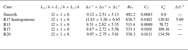
 Lx/h×Ly/h×Lz/h
 Δx+
Δx+ Δy+
Δy+ Δz+
Δz+

 ⟨u⟩/Ubh
 (y−y0)/h
 ⟨u⟩+
⟨u⟩+ (y−y0)+
 H
H y0
y0 h=H−y0
 Ubh
Ubh h
h δν=ν/uτ
 urms/uτ
 vrms/uτ
 wrms/uτ
 (y−y0)/h
 ⟨u′v′⟩/uτ2
 (y−y0)/h
 τijDA
τijDA τ11DA
τ11DA τ22DA
τ22DA τ33DA
τ33DA −τ12DA
 uτ2
uτ2 (y−y0)+
 y
y z
z y
y z
z (y−y0)+
 U¯/Ub
U¯/Ub
 Λci∗
Λci∗ Ωx
Ωx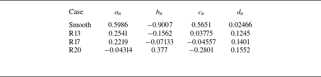
 an
an bn
bn cn
cn dn
dn σ
σ
 ⟨NCP⟩
⟨NCP⟩ LCP/Lx
 LCP/h⩾3
 LCP/Lx
 LCP/Lx
 LCP/h
LCP/h u
u u
u ⟨NCP⟩+/−
 (LCP,y)
 u−⟨u¯⟩
 x
x z
z y/h=0.3
 R(uI′,u′)
 y
y z
z
 R(uI′,w′)
 y
y z
z R(uI′,v′)
 y/h=0.15
 kxFuu(kx)/uτ2
 |kxCuv(kx)|/uτ2
 λx/h
λx/h z/h=2.4
 z/h=3.0
 z/h=3.6
 (y+,λz+)
 y0
y0 λz=5y
λz=5y λz=5η
λz=5η η
η
 (y/h,λz/h)
 y0/h
y0/h
 (y+,λz/h)
 λz/h=O(1)
 y/h∈[0,0.3]
 y/h∈[0.3,1.0]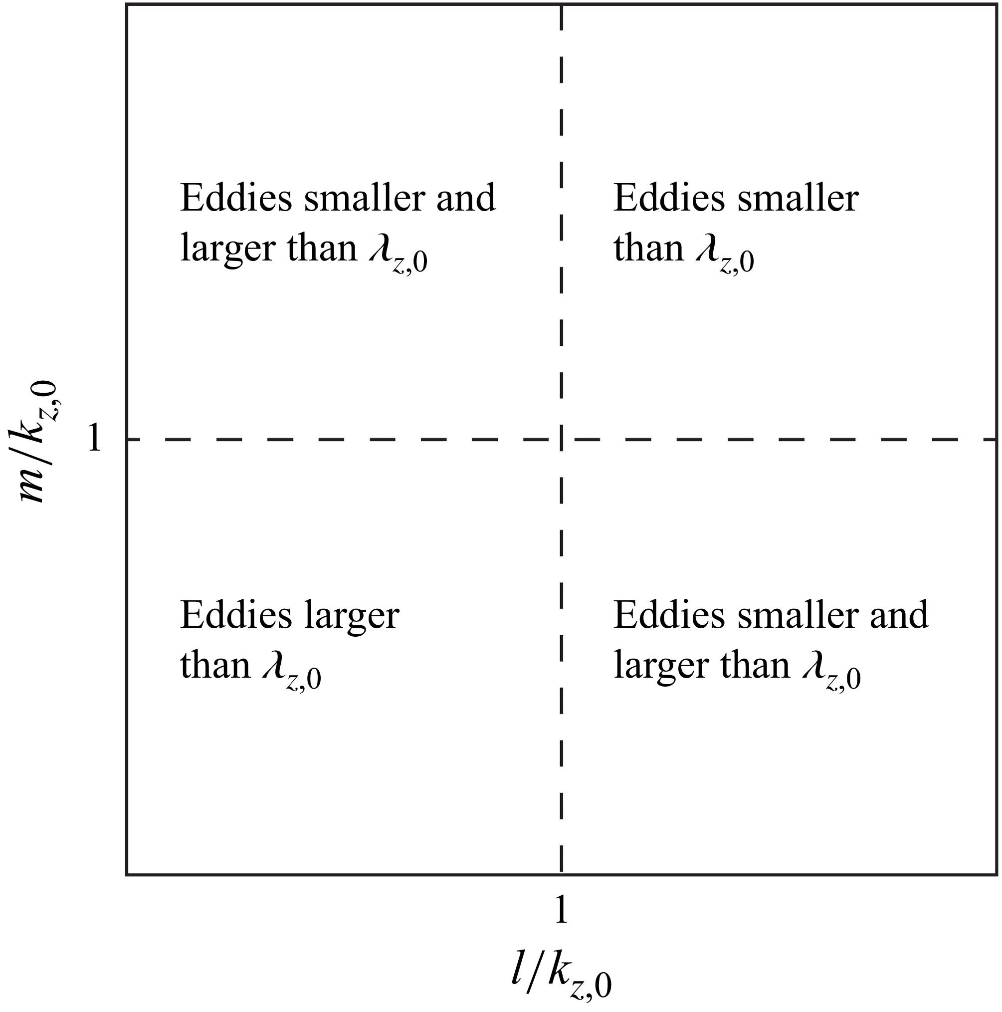
 (l/kz,0,m/kz,0)
 λz,0=2π/kz,0
 l/kz,0=1
 m/kz,0=1
 λz,0
λz,0
 (l/kz,0,m/kz,0)
 l/kz,0=1
 m/kz,0=1
 (l/kz,0,m/kz,0)
 (l=m)
(l=m) kz,0
kz,0

 ⟨NCP⟩
⟨NCP⟩ LCP/Lx
 Lx/h=12
 Lx/h=24
 u
u
 Lx/h=24
 kxFuu(kx)/uτ2
 |kxCuv(kx)|/uτ2
 y/h=0.7
 y/h=0.3
 z/h=2.4
 3.0
3.0 3.6
3.6
 Lx/h=12
 λz/h≈0.3
 Lx/h=24
 λz/h=O(1)
 (l/kz,0,m/kz,0)
 kz,0
kz,0
 ISC(y)=⟨V2+W2⟩z/Ub
 V
V W
W ⟨⋅⟩z
⟨⋅⟩z Reτ≈533
 Reτ≈300
 Reτ
Reτ
 Reτ≈533
 Reτ≈300
 U/Ub
U/Ub (W,V)
(W,V) Reτ
Reτ
 Reτ≈533
 Reτ≈300
 Λcisgn(Ωx)
 (W,V)
(W,V)
 Open access

