2. Simulation model and parameters of compressible convection

The equations of motion for compressible convection are given by

(2.1)\begin{gather} \partial_t \rho + \partial_i (\rho u_{i}) = 0, \end{gather}

(2.2)\begin{gather}\partial_t (\rho u_{i}) + \partial_j (\rho u_{i} u_{j}) ={-}\partial_i p + \partial_j \sigma_{ij} - \rho g \delta_{i,3} , \end{gather}

(2.3)\begin{gather}\partial_t (\rho e) + \partial_j (\rho e u_{j} ) ={-}p \partial_i u_{i} + \partial_i(k \partial_i T) + \sigma_{ij} S_{ij}, \end{gather}

(2.4)\begin{gather}p = \rho R T \quad\text{where }\ R= C_{p} -C_{v} . \end{gather}

These equations correspond to mass, momentum and energy conservation laws along with the ideal gas equation of state. Here, $\rho$, $\rho u_{i}$, $p$, $\rho e$, $T$ are the mass density, momentum density components, pressure, internal energy density and temperature, respectively. The acceleration due to gravity is g, viscous stress tensor is ${\boldsymbol {\sigma }}=2\mu {\boldsymbol S}+ 2\mu {\boldsymbol I}({\boldsymbol {\nabla }}\boldsymbol {\cdot } {\boldsymbol u})/3$ with the Kronecker tensor ${\boldsymbol I}$ and the rate of strain tensor ${\boldsymbol S} = ({\boldsymbol {\nabla }} {\boldsymbol u}+{\boldsymbol {\nabla }} {\boldsymbol u}^{\rm T})/2$. Here, $\boldsymbol{u}$ stands for the velocity field in vector notation. The dynamic viscosity $\mu$ is assumed to be constant in these simulations. The thermal conductivity $k$ is related to the viscosity through the Prandtl number, $k= \mu C_{p}/Pr$. In our DNS, $Pr= 0.7$; $C_{p}$ and $C_{v}$ correspond to specific heat at constant pressure and volume, respectively. Their ratio, $\gamma = C_{p}/C_{v}= 1.4$ for a diatomic gas. The internal energy is defined as $e=C_{v}T$.

A uniform grid is used in $x$- and $y$-directions along with periodic boundary conditions. In wall-normal $z$-direction, a non-uniform grid with a point clustering near the walls is taken, which follows a hyperbolic tangent stretching function. Spatial derivatives are calculated by a 6th-order compact scheme for all points except near the walls (Lele Reference Lele1992; Baranwal, Donzis & Bowersox Reference Baranwal, Donzis and Bowersox2022); 4th- and 3rd-order compact schemes are used at the last two grid points near the wall. No-slip, isothermal boundary conditions are applied at the top and bottom. The boundary condition for $p$ is evaluated using the $z$-component of the momentum equation at $z=0, H$, $\partial p/\partial z = \left( \partial \sigma_{iz}/\partial x_{i} \right) - \rho g$. The fields are advanced in time by a low-storage 3rd-order Runge–Kutta with a Courant number of ${\rm CFL}=0.5$.

Incompressible Rayleigh–Bénard convection is determined by the Rayleigh and Prandtl numbers, $Ra$ and $Pr$. In compressible convection, additional dimensionless parameters need to be introduced. The first one is the dissipation number $D$ (Verhoeven et al. Reference Verhoeven, Wiesehöfer and Stellmach2015; Jones et al. Reference Jones, Mizerski and Kessar2022) which is given by

(2.5)\begin{equation} D= \frac{gH}{C_{p}T^{B}}. \end{equation}

The parameter $D$ can be considered as a rescaled dry adiabatic lapse rate as it determines differences in the thermodynamic properties across the layer depth in a purely isentropic process. The adiabatic temperature ratio between top (T) and bottom (B) is $T^{T}_{a} /T^{B}_{a}=( 1 - D)$, the corresponding density ratio follows to $\rho ^{T}_{a} /\rho ^{B}_{a} = [ T^{T}_{a} /T^{B}_{a} ]^{1/ ( \gamma -1 ) }$. The subscript ‘$a$’ corresponds to the adiabatic equilibrium without convection. The equilibrium profiles for all state variables and all values of $D$ are shown in figure 1. In order to initiate convective motion, the actual temperature gradient across the layer must be greater than that due to a purely adiabatic process (Jeffreys Reference Jeffreys1930), i.e. $T^{B} - T^{T} > T_{a}^{B} - T_{a}^{T}$. In our study, the bottom plate is taken as the reference, thus $T^{B}= T_{a}^{B}$ is a constant for all cases; the instability criterion reduces to $T^{T} < T_{a}^{T}$.

Figure 1.

Adiabatic equilibrium profiles of the thermodynamic state variables. (a) Temperature $T$, (b) density $\rho$ and (c) pressure $p$. The difference between top and bottom values for all three variables increases with $D$, see table 1 for the colour code description.

The second additional compressible convection parameter is the superadiabaticity $\epsilon$ (Verhoeven et al. Reference Verhoeven, Wiesehöfer and Stellmach2015; Jones et al. Reference Jones, Mizerski and Kessar2022) , which is given by

(2.6)\begin{equation} \epsilon= \frac{T_{a}^{T} - T^{T}}{T^{B}}. \end{equation}

Superadiabaticity is the excess relative temperature gradient with respect to the adiabatic equilibrium state, or, in other words, a measure of the driving of convection. If one takes the characteristic free-fall velocity, $U_{f}= \sqrt {\epsilon g H}$, then a free-fall Mach number,

(2.7)\begin{equation} M_{f}(z) = \frac{U_{f}}{\sqrt{\gamma R \langle T(z) \rangle_{A,t}}} = \sqrt{\frac{\epsilon D}{\gamma - 1}} \sqrt{\frac{T^{B}}{\langle T(z)\rangle_{A,t}}} , \end{equation}

follows. The notation $\langle \boldsymbol {\cdot }\rangle _{A,t}$ corresponds to a combined average over the horizontal directions and time which is given for a field $X$ as

(2.8)\begin{equation} \langle X (z) \rangle_{A,t} = \frac{ \displaystyle\sum^{N_{t}}_{m=1} \displaystyle\sum^{N_{x}}_{i=1} \sum^{N_{y}}_{j=1} X(x_i, y_j,z,t_m)}{N_{x}N_{y}N_{t}}, \end{equation}

where $N_{x}$, $N_{y}$ and $N_{t}$ are the grid point numbers with respect to $x$-, $y$-directions and number of snapshots, respectively. The strength of compressibility is thus a function of both $\epsilon$ and $D$. From (2.7), it is expected that compressibility at the top is higher than at the bottom. For $\epsilon \rightarrow 0$, we get the anelastic approximation which includes first-order terms in $\epsilon$ only (Ogura & Phillips Reference Ogura and Phillips1962; Gough Reference Gough1969; Lantz & Fan Reference Lantz and Fan1999). This results in a filtering of high-frequency acoustic waves. Rayleigh–Bénard convection in the Oberbeck–Boussinesq (OB) limit follows for a subsequent $D \rightarrow 0$ with $D$ decreasing faster than $\epsilon$. On the basis of the new parameters, we will use $Ra= \epsilon g H^{3}/(\nu ^{B} \kappa ^{B})$ and Prandtl number, $Pr= \nu ^B/\kappa ^B$, where $\kappa ^B= k/(C_{p} \rho _a^B )$ is the temperature diffusivity and $\nu ^B=\mu /\rho _a^B$ the kinematic viscosity. The Rayleigh number is here defined with respect to the bottom variables and thus constant for all cases. Unlike $Ra$, which varies across depth due to density dependence, Prandtl number $Pr$ is a constant in the entire domain, since the density drops out for $\nu$ and $\kappa$. In this work, we focus on a constant and low but finite superadiabaticity, $\epsilon =0.1$ for a range of $D$ from $0.1$ to $0.8$. All other governing parameters such as $Ra \approx 10^6$, $Pr= 0.72$ and aspect ratio, $\varGamma = 4$ are kept constant, see table 1. In all figures that follow, unless specified otherwise, we use the plotting style given in the last column. From table 1, we observe that in our study, the strength of density stratification $(\rho _{a}^{B}/\rho _{a}^{T})$ ranges from 1.3 at $D= 0.1$ to 55.9 at $D=0.8$. The degree of stratification in previous compressible convection simulations is thus significantly smaller than what we will study here. The strongest stratification ratios in Verhoeven et al. (Reference Verhoeven, Wiesehöfer and Stellmach2015), Jones et al. (Reference Jones, Mizerski and Kessar2022), and Tilgner (Reference Tilgner2011) are 20.1, 10 and 4.6, respectively.

Table 1.

List of the DNS. All cases have $Pr= 0.7$, $Ra \approx 10^6$, $\epsilon = 0.1$, $\gamma = C_{p}/C_{v}= 1.4$, and an aspect ratio, $\varGamma =L/H=4$ resolved by $N_x:N_y:N_z=512: 512: 256$ grid points. Here, L is the horizontal domain size. We list dissipation number $D$, bottom-to-top ratios of adiabatic temperatures and densities, the global maximum turbulent Mach number $M_t^{max}$, the Nusselt and Reynolds numbers, $Nu$ and $Re$. The error bars of $Nu$ and $Re$ are less than $2\,\%$ for all cases. Furthermore, we display boundary-layer scales for density, convective heat flux and density–temperature correlations. In all figures that follow, coloured lines are given as in this table.

3. Growing asymmetry with increased stratification

The adiabatic temperature profile, $T_{a}(z)=T^B_a(1-Dz)$, is the equilibrium profile. Thus the part of temperature corresponding to convection is the superadiabatic temperature defined as

(3.1)\begin{equation} T_{sa} ({\boldsymbol x},t)= T({\boldsymbol x},t) - T_{a}(z). \end{equation}

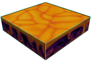
In figure 2, we compare the contour visualization of $\ln (| \boldsymbol {\nabla } T_{sa}| )$ for the two extreme cases in our series with $D= 0.1$ (low) and $D= 0.8$ (high). Panel (a) corresponds to case 1, closest to the OB limit. Not surprisingly, the plumes from the top and bottom are more or less symmetric in shape and frequency. However, this top-bottom symmetry disappears completely for the highly stratified case 8 in panel (b). One observes a network of slender thin plumes (Rast Reference Rast1998) originating from the top boundary layer that fall deep into the bulk. Recently, John & Schumacher (Reference John and Schumacher2023) showed that thinner plumes from the top boundary are a common characteristic of compressible convection regardless of the relative boundary-layer thickness, but here the asymmetry is very pronounced.

Figure 2.

Visualization of the plume structure of the superadiabatic temperature field $T_{sa}$. Contours of $\ln |{\boldsymbol \nabla } T_{sa} |$ are shown at two instants, (a) for case 1 with $D=0.1$ and (b) for case 8 with $D=0.8$. Minimum/maximum contour levels correspond to $-7.0/-2.4$ in (a) and $-9.5/-4.0$ in (b). The top contour surface is slightly below $z=H$.

Similar asymmetry is observed for the mean profile of the superadiabatic temperature, $\langle T_{sa} (z) \rangle _{A,t}$. In figure 3(a), we plot the normalized superadiabatic temperature, $\langle T_{sa}(z)\rangle _{A,t}/ \varDelta \langle T_{sa} \rangle _{A,t}$ as a function of depth $z$ where $\varDelta \langle T_{sa} \rangle _{A,t}=\langle T_{sa}(z=0) \rangle _{A,t} - \langle T_{sa}(z=H) \rangle _{A,t}$. Clearly one observes that the asymmetry, i.e. the offset from 0.5 and thickness of the top boundary layer in comparison with the bottom one, increases considerably with growing dissipation number. More detailed, as $D$ increases, the bulk temperature is increasingly closer to the bottom temperature, consistent with Tilgner (Reference Tilgner2011), Verhoeven et al. (Reference Verhoeven, Wiesehöfer and Stellmach2015), Jones et al. (Reference Jones, Mizerski and Kessar2022) or Curbelo et al. (Reference Curbelo, Duarte, Alboussière, Dubuffet, Labrosse and Ricard2019) for $Pr\to \infty$. Differently, the experiments of Wu & Libchaber (Reference Wu and Libchaber1991) showed that the bulk temperature is closer to the prescribed top plate value with $(\nu ^{T}, \kappa ^{T} ) < ( \nu ^{B}, \kappa ^{B} )$. This results in a thinner top boundary layer and a bulk temperature closer to that at the top. Due to strong density stratification, we get $(\nu ^{T}, \kappa ^{T} ) > ( \nu ^{B}, \kappa ^{B} )$ and thus thicker layers at the top, which is detailed later. A trend similar to Wu & Libchaber (Reference Wu and Libchaber1991) is observed for $\epsilon / D \gg 1$ in John & Schumacher (Reference John and Schumacher2023).

Figure 3.

Asymmetry of the (a) normalized superadiabatic temperature and (b) the turbulent Mach number $M_t$. The inset in (a) corresponds to mean thermal boundary-layer thickness $\lambda ^{B,T}(D)$. Symbols $+$ and ${\rm o}$ are for the top and bottom boundary-layer thickness, respectively. The inset in (b) shows $M_f(D)$ from (2.7). The red, blue and green lines are for $z/H = 0, 1$ and 0.5, respectively. The black squares are the maximum Mach numbers as given table 1, which are observed in the simulations over the whole space and time. The legend in (b) corresponds to the inset figure.

We can quantify this thickness as the mean of a local thermal boundary-layer thickness (Scheel & Schumacher Reference Scheel and Schumacher2014) which is given by

(3.2) \begin{equation} \tilde{\lambda}^{B,T}(x,y)= \frac{1}{H}\left | \langle T_{sa} \left( 0,H \right) - T_{sa} \left( H/2 \right) \rangle_{A,t} \right| \left | \frac{\partial {{T_{sa}} _{A,t}} }{\partial z} \right|^{{-}1} _{z=0,H}. \end{equation}

We plot $\lambda ^{B,T}=\langle \tilde {\lambda }^{B,T}\rangle _{A,t}$ as a function of $D$ in the inset of figure 3(a). The difference between the boundary-layer thickness at the bottom and top plate increases with $D$ in agreement with the differences observed in the distributions of the instantaneous, local thermal boundary-layer thicknesses (John & Schumacher Reference John and Schumacher2023). The top boundary-layer thickness increases drastically with $D$ whereas the bottom boundary-layer thickness is almost invariant. This, along with increased asymmetry in the bulk towards the bottom plate, as seen in the normalized $T_{sa}$-profiles, suggests that at high $D$ the mixing is not as efficient as in OB and compressibility effects are mainly localized near the top boundary.

An asymmetry similar to that of $\langle T_{sa}(z)\rangle _{A,t}$ is observed for the turbulent Mach number too with significant localized compressibility seen near the top boundary. The turbulent Mach number is defined as

(3.3)\begin{equation} M_{t}(z) = \frac{u_{ rms}(z)}{\sqrt{\gamma R \langle T(z) \rangle_{A,t}}}\quad \mbox{with} \quad u_{ rms}(z)= \sqrt{ \sum_{i=1}^3 \left [\langle u_{i}^{2}(z)\rangle_{A,t} - \langle u_{i}(z) \rangle^{2}_{A,t}\right ]}. \end{equation}

The turbulent Mach number at the top increases monotonically with $D$, whereas the behaviour at the bottom boundary is non-monotonic with $D$. At the bottom, $M_{t}$ increases up to $D= 0.5$ and then decreases with $D$ as a result of the increased asymmetry between the boundary layers, see figure 3(b).

In the inset of figure 3(b), we compare the resulting maximum turbulent Mach number in the flow with the estimate from (2.7). The black squares are the maximum local turbulent Mach number for each $D$ encompassing all time steps and spatial locations. The red and blue lines correspond to $M_{f}$ estimates using the bottom and top temperatures, $T^B$ and $T^{\rm T}$, respectively. One finds that the resulting maxima of $M_t$ are between these estimates. This is due to no-slip boundary conditions at the wall; thus, the velocity fluctuations peak only at the outer region of the boundary layer and in the bulk. Since the (mean) bulk temperature is closer to that at the bottom plate, the values of $M_t$ are closer to $M_{f} (T^{B} )$. A really close agreement for the simulations is seen when the Mach number is estimated using the bulk temperature, green line in the inset figure. This suggests that a simple estimate such as in (2.7) can give us a good idea about the level of compressibility in the flow.

We would like to point out that in compressible turbulence $M_{t}$ is not sufficient to characterize the system; an additional parameter $\delta$, the ratio of dilatational to solenoidal root-mean-square velocities, needs to be included as discussed in Donzis & John (Reference Donzis and John2020), John, Donzis & Sreenivasan (Reference John, Donzis and Sreenivasan2019, Reference John, Donzis and Sreenivasan2020, Reference John, Donzis and Sreenivasan2021). This is not surprising as in compressible convection two extremely different conditions, $\epsilon /D \ll 1$ and $\epsilon /D \gg 1$, can lead to the same $M_t$ despite different dynamics. John & Schumacher (Reference John and Schumacher2023) showed that an increasing $\epsilon$ leads to enhanced heat transfer, whereas it is decreased for increasing $D$ at low $\epsilon$. Even though $M_t$ would be comparable for both cases, $\delta$ will differ in these limits. A similar conclusion, that the Mach number along with a measure of dilatation in the flow field is required for the statistical analysis, was reported for compressible turbulent channel flows (Baranwal, Donzis & Bowersox Reference Baranwal, Donzis and Bowersox2023a,Reference Baranwal, Donzis and Bowersoxb).

4. Fluctuations of state variables and regime transition

A major consequence of compressibility are the fluctuations of $p$, $\rho$ and $T$. In figure 4, we compare these fluctuations as a function of depth for the two extreme cases of our DNS series, $D= 0.1$ and $0.8$. John & Schumacher (Reference John and Schumacher2023) showed that $D\le 1-\epsilon$, which would result in a maximally possible theoretical value of $D=0.9$ in our DNS series. The relative fluctuations are defined as $X_{ rms}(z)/\langle X(z) \rangle _{A,t}$ with $X_{ rms} = (\langle X^2 \rangle _{A,t} - \langle X \rangle _{A,t}^2)^{1/2}$. Panel (a) at $D=0.1$ shows that pressure fluctuations are negligible. The magnitude of the density and temperature fluctuations are of the same order of magnitude and the profiles of both quantities are practically identical. These findings are consistent with the OB limit at $\epsilon, D \rightarrow 0$.

Figure 4.

Relative fluctuations of thermodynamic quantities for (a) $D = 0.1$ and (b) $D= 0.8$. (c) Maximum of the relative thermodynamic fluctuations vs dissipation number, $D$. For all figures, the red, blue and green correspond to temperature, density and pressure, respectively. Inset of (c) shows four different distances $\lambda _{X}$ as a function of $D$. For the definition of the specific $\lambda _{X}$, we refer to the text in § 4 and the legend of the inset.

In figure 4(b), the relative fluctuations of $p$, $\rho$ and $T$ at $D= 0.8$ are shown. As a result of high compressibility at $D=0.8$ at the top, see figure 3(b) for $M_t(z)$, the thermodynamic fluctuations are considerably higher compared with the bottom one. Close to the top boundary, the pressure and density fluctuations dominate the temperature fluctuations. This is due to the constant temperature imposed at the boundaries which results in an isothermal condition. For an assumed ideal gas, $p\propto \rho$. Indeed this is evident for $D= 0.8$ at the top boundary as the relative fluctuations of density and pressure perfectly match at the top boundary. This would be also true at the bottom boundary and even for $D=0.1$, but it is not evident due to low $M_{t}$. Compressibility effects imply in the following discussion that we face a large magnitude of pressure fluctuations.

As we move away from the wall, fluctuations of both $p$ and $\rho$ decrease, but are not perfectly correlated anymore due to the growing temperature fluctuations. After a critical distance from the wall, pressure fluctuations continue to decrease; the density fluctuations reach a minimum at $z=z_{\ast }$. This local minimum of $\rho _{ rms}(z)/\langle \rho (z)\rangle _{A,t}$ exists when pressure and temperature fluctuations become comparable in magnitude. For the highest dissipation number $D= 0.8$, density fluctuations at $z< z_{\ast }$ are driven by temperature fluctuations in contrast to $z>z_{\ast }$. One also notes that the location of the secondary maximum of $\rho _{ rms}(z)/\langle \rho (z)\rangle _{A,t}$ does not match the local maxima of $T_{ rms}(z)/\langle T(z)\rangle _{A,t}$. This implies that pressure fluctuations, although not dominant, remain significant and thus compressibility effects too (Jones et al. Reference Jones, Mizerski and Kessar2022).

These features are absent for $D= 0.1$ in figure 4(a). Thus, there seems to exist a critical $D$ where a transition to the compressibility dominated convection regime exists that is qualitatively different to the OB or anelastic limits. In order to identify the critical $D$, we plot the maximum relative thermodynamic fluctuations with respect to $D$ in figure 4(c). We find a $D_{ crit}\approx 0.65$ for the present $(Ra,\epsilon )$. For $D < D_{ crit}$, maxima of density and temperature fluctuations dominate over those of the pressure fluctuations. As $D$ increases, the maximum pressure fluctuations start to increase as well which is connected with increasing differences in the maxima of density and temperature fluctuations. For $D \ge D_{ crit}$, the maxima of pressure and density fluctuations collapse and are larger than those for the temperature fluctuations.

Clearly, there are multiple physical processes and thus scales at play near the top boundary at high $D$. This seems to be similar to the turbulent boundary layer with its inner and outer scales (Smits, McKeon & Marusic Reference Smits, McKeon and Marusic2011). The behaviour of density can be analysed to demarcate various regimes inside the boundary layers in compressible convection. We thus introduce the following boundary layer scales: (1) $\lambda _{T_{ max}}$ as the distance between the top wall and the location of the local maximum of the relative temperature fluctuations; (2) $\lambda _{\rho _{ max}}$ as the distance between the top wall and the maximum of the relative density fluctuations. Note that in OB and even anelastic convection, $\lambda _{T_{ max}} = \lambda _{\rho _{ max}}$ (Jones et al. Reference Jones, Mizerski and Kessar2022). Furthermore, (3) $\lambda _{\rho _{ min}}$ as the distance between the top wall and the location of the local minimum of the relative density fluctuations. This distance corresponds to the location where we start to observe significant compressibility effects. Finally, (4) $\lambda _{\rho _{{ max},T}}$ is the distance between the top wall and the local maximum of the relative density fluctuations, corresponding to the maximum of local temperature fluctuations.

Next, we display all four scales $\lambda _X$ vs $D$ in the inset of figure 4(c). Here $\lambda _{T_{ max}}$ increases with $D$ which is consistent with the growth of the thermal boundary-layer thickness at the top, $\lambda ^{T}$, see figure 3(a). We see a sudden transition of $\lambda _{\rho _{ max}}$ at $D_{crit}= 0.65$ indicating that the maximum for $D>D_{ crit}$ is at $z=H$. Note also that for $D < 0.65$, $\lambda _{\rho _{ max}} \approx \lambda _{\rho _{{ max}, T}}$. Both scales increase with $D$, but start to deviate from $\lambda _{T_{ max}}$ at $D < D_{ crit}= 0.65$. This deviation starts for $D \ge 0.5$; it suggests that pressure fluctuations are important already, but not as dominant as discussed before. It might thus indicate that the anelastic approximation is strictly speaking not applicable even for $D \ge 0.5$. Finally, $\lambda _{\rho _{ min}}$ starts from nearly zero at $D = 0.1$ with negligible compressibility. With increasing dissipation number, $\lambda _{\rho _{ min}}$ increases. This is a new top boundary-layer regime induced by the increasing stratification. It is in line with an increase of $\lambda _{T_{ max}}$ and $\lambda ^{T}$; see again the inset of figure 3(a). We discuss the implications of this sublayer for the turbulent heat transfer in the next section.

5. Stratification impact on turbulent heat transfer

A systematic increase of the level of stratification, controlled by $D$, at relatively small superadibaticity of $\epsilon = 0.1$ has a significant impact on the normalized stress profiles as seen in figure 5. We show the variation of the normalized convective heat flux profiles $J_c(z)$ in panel (a) and the normalized density–temperature correlation profiles $J_{\rho }(z)$ in panel (b) for all eight runs. They are qualitatively similar, but sign-flipped behaviour is observed for both second-order correlations in panels (a,b). An increasing sublayer with an average ‘anti-convection’-behaviour, i.e. negative convective heat flux and positive density–temperature correlation can be detected. Note that $J_{\rho }(z)$ is only present in fully compressible convection and neglected in the anelastic case. Exactly, this term becomes significant for the highest $D$ and is expected to further increase when $D\to 0.9$ (which is computationally very hard). For $z\lesssim 0.9$ ($D= 0.8$) both mean profiles correspond to unstable convection.

Figure 5.

Profiles of plane-time averaged stresses vs $D$. (a) Normalized convective heat flux $J_{c}(z)= \langle u_z T^{\prime }(z)\rangle _{A,t}/[u_{z,{rms}}(z)\langle T(z)\rangle _{A,t}]$. (b) Normalized density–temperature correlation $J_{\rho }(z)=\langle \rho ^{\prime } T^{\prime }(z)\rangle _{A,t}/[\langle \rho (z)\rangle _{A,t}\langle T(z)\rangle _{A,t}]$. (c) Normalized density averaged convective heat flux where $J^{\rho }_{c}(z)=\langle \rho u_z T^{\prime }(z)\rangle _{A,t}$ and (d) Nusselt number $Nu$ vs dissipation number $D$, see (5.1). Inset of (d) displays $1/Nu$ vs $\lambda _{\rho _{min}}$. The dashed line corresponds to a fit $A + B \lambda _{\rho _{ min}}$ with coefficients $A=0.12$ and $B=1.05$. Line colouring corresponds to table 1. Note that $T^{\prime }$ follows by a standard Reynolds decomposition, $T({\boldsymbol x},t)=\langle T(z)\rangle _{A,t}+T'({\boldsymbol x},t)$.

Next, we relate the depth of these stabilized regions to $\lambda _{\rho _{ min}}$ and thus to the regime transition at $D=D_{ crit}$. We therefore define three further distances or scales: (1) $\delta _{u_{z}T}$ as the width of negative normalized heat flux with respect to the top boundary; (2) $\lambda ^{max}_{\rho 'T'}$ as the distance from the top boundary to the location of the positive maximum of the normalized density–temperature correlation; (3) $\delta _{\rho 'T'}$ as the width of the region of positive density–temperature correlations.

These length scales along with $\lambda _{\rho _{ min}}$ are listed in table 1 for all DNS. We observe that for all runs, except for $D= 0.1$, the region of positive correlation exactly matches with the compressibility dominated region, i.e. $\delta _{\rho 'T'}=\lambda _{\rho _{ min}}$. Thus, there is also a direct proportionality between regions dominated by compressibility and anti-convection with $\delta _{{u_z}T} < \lambda _{\rho _{ min}}$. For $D \le 0.70$, we also find that $\delta _{{u_z}T} \approx \lambda ^{max}_{\rho 'T'}$, the location of the maximum positive correlation. For $D > 0.7$, we get $\delta _{{u_z}T} > \lambda ^{max}_{\rho 'T'}$, suggesting an increasing influence of compressibility. Furthermore, $\delta _{{u_z}T} < \lambda _{\rho _{ min}}$ implies that on average weak convective motions can occur at heights, $\lambda _{\rho _{ min}}\gtrsim z\gtrsim \delta _{{u_z}T}$, even though there are already significant compressibility effects. We recall for this discussion that even for the highest $D$, we still observe focused cold thermal plumes which detach from the top thus indicating locally positive convective flux. All these processes take places in the region where density fluctuations are tightly correlated to pressure fluctuations as we discussed in figure 4(c). We also report that there is no trend of the location of maximum turbulent Mach number, $M^{\ast }_{t}=\max _z M_t(z)$, see figure 3(b), with $D$ even though $M_{t}^{\ast }$ increases with $D$. For all the cases considered, the distance of this maximum to the top wall is $H-z_{\ast } \in [0.16, 0.174]$, significantly larger than $\lambda _{\rho _{ min}}$. This again suggests the inadequacy of $M_{t}$ alone to characterize general compressibility conditions (Donzis & John Reference Donzis and John2020). Particularly for the strongly asymmetric cases at highest $D$, the behaviour of compressible convection is completely different for same $M_{t}$ magnitude at either side of $z_{\ast }$.

In figure 5(c) we also plot the plane-averaged heat flux, $J^{\rho }_{c}(z)=\langle \rho ' u_z T'\rangle _{A,t}$, normalized by the maximum value. We observe a region of practically zero convective heat flux near the top that increases with $D$. For $z>H-\delta _{u_{z}T}$, the flux $J^{\rho }_{c}$ is less than 1 % of its maximum. There are other ways to define convective flux in terms of entropy or enthalpy (Currie & Browning Reference Currie and Browning2017). The entropy changes can written as $\rho T dS = \rho C_{p} \,{\rm d}T - {\rm d}P$. The pressure term is neglected when boundary layers are incompressible. At high $D$, the boundary layer near the top is, however, strongly compressible. We consider the contributions due to pressure changes as a genuine compressibility effect; they become important and we analysed them in this work separated from the convective flux.

Finally, we plot the Nusselt number defined as

(5.1)\begin{equation} Nu = \frac{1}{2} \left[\left . - \frac{H}{\epsilon T_{B}} \frac{{\rm d} \langle T_{sa} \rangle _{A,t}}{{\rm d}z} \right|_{z=0} \left . - \frac{H}{\epsilon T_{B}} \frac{{\rm d} \langle T_{sa} \rangle _{A,t}}{{\rm d}z} \right|_{z=H}\right]. \end{equation}

It is shown as a function of $D$ in figure 5(d). The Nusselt number is calculated as the average of the heat flux at the top and bottom. Since the flows are statistically steady, the Nusselt number at the top and bottom are the same and the maximum mean Nusselt number difference between the plate is found to be less than $3\,\%$ for all cases. Clearly visible is that the Nusselt number $Nu$ monotonically decreases with $D$. At critical $D= 0.65$, there seems to be a slight change in behaviour but it is not significant. A decrease of $Nu$ with $D$ is again consistent with previous studies (Verhoeven et al. Reference Verhoeven, Wiesehöfer and Stellmach2015; Jones et al. Reference Jones, Mizerski and Kessar2022). We plot the inverse of the Nusselt number vs $\lambda _{\rho _{ min}}$ in the inset of panel (d) and we observe that the trend can be reasonably approximated by a linear fit. Thus, we conclusively demonstrate that an increasingly inefficient heat transfer is connected to structural changes in the top boundary layer.

6. Final discussion

The objective of the present study was to take the least complex, but fully compressible turbulent convection system to study the genuine effects of compressibility isolated from other major contributions to a non-Boussinesq behaviour, such as temperature-dependent material properties, and to go beyond the OB and anelastic limits. We took a configuration in the limit of strongly decreasing mean profiles of the thermodynamic state variables – the high stratification regime. It corresponds to the dissipation number of $D\to 1$ for small superadiabaticity $\epsilon$. One prominent example for such a configuration might be the convection dynamics close to the solar surface. Even though the aim of our work is not to provide a realistic modelling of particularly this complex multi-physics flow, that would involve the coupling to magnetic fields and radiation transfer, the present simulations provide an insight into generic physical mechanisms which lead to highly asymmetric thermal plume motions, the fundamental local process in any convection flow that triggers fluid turbulence and transports heat. The limit cases of our simplified configuration lead already to a sparse network of thin plume structures which resembles similarities to the granule network at the Sun; see again figure 2(b). These coherent structures ‘leak’ through the stratified top region and thus maintain a significantly reduced global turbulent heat transport. Future studies will aim at an increase of the aspect ratio and Rayleigh number together with a decrease of the Prandtl number and $T$-dependent material parameters.