





1. Introduction
Flying insects’ wings rapidly shed vortices that interact to form a highly complex, three-dimensional (3-D), and unsteady aerodynamic wake. Understanding the wake dynamics is central to explaining the remarkable efficiency, stability and manoeuvrability inherent to insect flight (Sane Reference Sane2003; Wang Reference Wang2005). Much progress has been made in this direction; one prominent discovery is the leading-edge vortex, which is essential for generating the high lift necessary for flight (Ellington et al. Reference Ellington, Van Den Berg, Willmott and Thomas1996). Similarly, other studies have highlighted clap-and-fling (Weis-Fogh Reference Weis-Fogh1973), wake capture (Dickinson, Lehmann & Sane Reference Dickinson, Lehmann and Sane1999) and other unsteady mechanisms that contribute to insects’ aerodynamic performance (Lehmann Reference Lehmann2004). However, beyond simply being a collection of discrete vortices and their interactions, the wake itself is a dynamically evolving system with its own emergent formation, stability and decay properties. Modelling the wake as a whole is a challenging prospect, largely due to the many degrees of freedom necessary for representing its individual components. For example, typical computational fluid dynamics (CFD) simulations involve of the order of 106 computational domain cells (Lionetti, Hedrick & Li Reference Lionetti, Hedrick and Li2022; Lou et al. Reference Lou, Lei, Dong and Li2024; Haider et al. Reference Haider, Lou, Hsu, Cheng and Li2025). Such complexity is a barrier to direct analysis and control strategies and motivates the need for reduced-order modelling (ROM) techniques to isolate the governing dynamics.
Reduced-order modelling provides a powerful suite of tools for simplifying high-dimensional fluid systems. A common first step is modal decomposition, a linear dimensionality reduction technique that expresses the flow as a set of spatial modes with time-varying amplitudes. Various decomposition algorithms have been introduced, each with its own specific aims and properties (e.g. proper orthogonal decomposition (POD), dynamic mode decomposition (DMD) and the discrete Fourier transform) (Taira et al. Reference Taira, Brunton, Dawson, Rowley, Colonius, McKeon and Ukeiley2017). Following decomposition, the next step is to identify a dynamic model governing the temporal evolution of the modal amplitudes. Traditionally, this is accomplished via Galerkin projection, wherein the Navier–Stokes equations are projected onto the modal basis to yield a system of ordinary differential equations (Holmes Reference Holmes2012). However, Galerkin approaches occasionally suffer from stability and closure issues, motivating a recent shift toward data-driven techniques (Schlegel & Noack Reference Schlegel and Noack2015; Callaham, Brunton & Loiseau Reference Callaham, Brunton and Loiseau2022). For example, sparse identification of nonlinear dynamics (SINDy) uses sparse regression to identify a parsimonious and interpretable model for the system dynamics (Brunton et al. Reference Brunton, Proctor and Kutz2016a ). Data-driven ROM strategies have been applied to a wide range of fluid dynamics problems, including bluff body wakes (Loiseau, Brunton & Noack Reference Loiseau, Brunton and Noack2021), plasma physics (Kaptanoglu et al. Reference Kaptanoglu, Morgan, Hansen and Brunton2021) and airfoil dynamics (Wang et al. Reference Wang, Zhang, Zhou, Sun and Wu2024). While such methods have proven powerful for canonical flows, their application to complex moving-boundary problems like insect flight has been more limited.
Prior applications of ROM techniques to insect flight have yielded numerous valuable insights, although certain questions pertaining to the wake dynamics remain unanswered. For example, modal decomposition studies have successfully identified dominant flow structures in 3-D flapping-wing wakes, although few have commented on the amplitude dynamics, long-term stability and energy transfer across modes (Liang & Dong Reference Liang and Dong2015; Li, Wang & Dong Reference Li, Wang and Dong2017). Other studies have focused on modelling the insect’s wing motion, flight manoeuvres and body oscillations (Liang & Sun Reference Liang and Sun2013; Hedrick, Blandford & Taha Reference Hedrick, Blandford and Taha2024); however, such approaches are limited to the insect’s kinematics and do not extend to the wake as a whole. Furthermore, quasisteady approaches, while enabling exploration of the dynamic properties of insect flight, do not yield models that can reproduce the wake’s transient evolution (Ellington Reference Ellington1984; Brunton, Rowley & Williams Reference Brunton, Rowley and Williams2013). Consequently, ROM of the spatio-temporal dynamics of the full insect wake remains an important, yet underexplored area.
To address these limitations, we employ data-driven ROM techniques to identify an interpretable model for a hovering hawkmoth’s wake. We begin by simulating hawkmoth flight using an in-house CFD solver. Then, we employ DMD to reduce the dimensionality of the resulting flow. Given that the DMD amplitudes exhibit strong nonlinear correlations, we use sparse regression to identify modal relationships and further reduce dimensionality, following Loiseau et al. (Reference Loiseau, Brunton and Noack2021) and Callaham et al. (Reference Callaham, Brunton and Loiseau2022). Finally, we leverage SINDy to construct a reduced-order dynamic model for the hovering hawkmoth’s wake. We validate the model by comparing its prediction of the hawkmoth’s aerodynamic forces with the simulated force history. Predicted forces are computed using an impulse-based wake survey method (Noca, Shiels & Jeon Reference Noca, Shiels and Jeon1997). Our overall modelling strategy is described by the flowchart in figure 1. The resulting model aims to provide a simple and physically interpretable representation of the wake’s evolution, elucidating the nonlinear mechanisms underlying energy transfer and stability in flapping-flight wakes.
Flowchart of the ROM process. (a) The hawkmoth’s wake is simulated via CFD. (b) The DMD extracts spatio-temporal modes from the flow data. (c) A sparse dynamic model is identified for the dominant modes using SINDy. (d) The model is validated by comparing its predicted aerodynamic forces, computed using the wake survey method, against the original simulation.

2. Methodology
2.1. Flow simulation of flapping flight
To obtain realistic flapping-wing kinematics for our simulation, we use wing motion data from our previous study (Lionetti et al. Reference Lionetti, Hedrick and Li2022). In that study, we recorded high-speed videos of a Manduca sexta hawkmoth hovering while feeding from an artificial flower, then transferred the recordings into Autodesk Maya to create a detailed 3-D reconstruction of the hawkmoth’s wing motion. This reconstructed model captures the natural bending and twisting deformations of the wings during flight. Full details of the experimental set-up, kinematic reconstruction procedure and wing Euler angle data can be found in Lionetti et al. (Reference Lionetti, Hedrick and Li2022).
We simulate hovering flight using an in-house immersed-boundary-method CFD solver. The solver numerically evaluates the unsteady 3-D viscous incompressible Navier–Stokes equations given by
 \begin{align}\boldsymbol{\nabla }\boldsymbol{\cdot }\boldsymbol{u}&=0,\nonumber\\ \frac{\partial \boldsymbol{u}}{\partial t}+\left(\boldsymbol{u}\boldsymbol{\cdot }\boldsymbol{\nabla }\right)\boldsymbol{u}&=-\frac{1}{\rho }\boldsymbol{\nabla }p+\nu {\nabla} ^{2}\boldsymbol{u},\end{align}
where $\boldsymbol{u}$
is the velocity, p is the pressure,
$\boldsymbol{u}$
is the velocity, p is the pressure, $\rho$
is the density and
$\rho$
is the density and $\nu$
is the kinematic viscosity. These equations are discretised in space using a second-order central differencing scheme, where the primitive variables
$\nu$
is the kinematic viscosity. These equations are discretised in space using a second-order central differencing scheme, where the primitive variables $\boldsymbol{u}$
and p are collocated at the cell centres. A fractional-step pressure-correction method is employed to advance the equations in time. Boundary conditions at the immersed bodies are enforced via a ghost-cell procedure (Mittal et al. Reference Mittal, Dong, Bozkurttas, Najjar, Vargas and Von Loebbecke2008), and movement of the immersed bodies (i.e. the flapping wings) is prescribed according to the aforementioned kinematic reconstruction. The Reynolds number used in the simulation is 7337, defined as Re =
$\boldsymbol{u}$
and p are collocated at the cell centres. A fractional-step pressure-correction method is employed to advance the equations in time. Boundary conditions at the immersed bodies are enforced via a ghost-cell procedure (Mittal et al. Reference Mittal, Dong, Bozkurttas, Najjar, Vargas and Von Loebbecke2008), and movement of the immersed bodies (i.e. the flapping wings) is prescribed according to the aforementioned kinematic reconstruction. The Reynolds number used in the simulation is 7337, defined as Re = $\overline{U_{\textit{tip}}}c/\nu $
, where
$\overline{U_{\textit{tip}}}c/\nu $
, where $\overline{U_{\textit{tip}}}$
= 4.9764 ms−1 is the average wing-tip velocity, c = 2.30 cm is the average wing chord length and
$\overline{U_{\textit{tip}}}$
= 4.9764 ms−1 is the average wing-tip velocity, c = 2.30 cm is the average wing chord length and $\nu$
= 1.56
$\nu$
= 1.56 $\times$
10–5 m2 s−1 is the kinematic viscosity of air.
$\times$
10–5 m2 s−1 is the kinematic viscosity of air.
Additional details regarding simulation set-up and grid independence are located in Appendix A, and our previous paper includes a validation based on force history (Lionetti et al. Reference Lionetti, Hedrick and Li2022). We run the simulation for a total of fifteen flapping cycles using identical wing kinematics for each cycle, thereby capturing the full evolution of the wake from quiescence at t/T = 0 to periodic steady state, where $T$
represents the period of one flapping cycle. This extended simulation duration is critical for developing a robust SINDy-based reduced-order model, as it provides a sufficiently rich dataset to capture both the transient and post-transient wake dynamics. In Appendix B, we demonstrate that the forces generated by the flapping wing become periodic after approximately five flapping cycles, while it takes nine cycles for the wake itself to achieve periodicity.
$T$
represents the period of one flapping cycle. This extended simulation duration is critical for developing a robust SINDy-based reduced-order model, as it provides a sufficiently rich dataset to capture both the transient and post-transient wake dynamics. In Appendix B, we demonstrate that the forces generated by the flapping wing become periodic after approximately five flapping cycles, while it takes nine cycles for the wake itself to achieve periodicity.
2.2. Dynamic mode decomposition
A wide variety of decomposition methods have been proposed for dimensionality reduction in fluid dynamics (Lumley Reference Lumley1967; Schmid Reference Schmid2010; Sieber, Paschereit & Oberleithner Reference Sieber, Paschereit and Oberleithner2016). In this work, we elect to use DMD for its ability to identify spatio-temporally coherent modes that oscillate with a fixed frequency. This attribute makes it ideal for studying flapping-wing wakes which are dominated by a single frequency (i.e. the hawkmoth’s flapping frequency, f = 25.6 Hz). Specifically, we employ the popular Exact DMD algorithm introduced by Tu (Reference Tu2013). Due to the widespread adoption of this method, we refrain from reproducing detailed derivations here, instead providing a brief overview of its theoretical foundations.
Dynamic mode decomposition approximates the eigendecomposition of the linear operator A that advances a system (in this case U , the fluid velocity components stored at all computational domain cells) forward in time
 \begin{equation}\,\boldsymbol{U}_{t+{\unicode[Arial]{x0394}} t}=\boldsymbol{A}\boldsymbol{U}_{t}.\end{equation}
However, for fluid dynamic systems, the dimensionality of
A
is often prohibitively large, making direct computation infeasible. Exact DMD therefore leverages the singular value decomposition to derive the reduced-order operator $\tilde{\boldsymbol{A}}$
. Spatial DMD modes are obtained from eigenvectors of
$\tilde{\boldsymbol{A}}$
. Spatial DMD modes are obtained from eigenvectors of $\tilde{\boldsymbol{A}}$
, and their temporal dynamics is determined by the corresponding eigenvalues. Each DMD mode is associated with a fixed frequency, growth/decay rate and initial amplitude. Based on this information, the time dynamics may be compiled into a coefficient matrix
$\tilde{\boldsymbol{A}}$
, and their temporal dynamics is determined by the corresponding eigenvalues. Each DMD mode is associated with a fixed frequency, growth/decay rate and initial amplitude. Based on this information, the time dynamics may be compiled into a coefficient matrix $\boldsymbol{\alpha }_{N\times M}$
, where N is the total number of modes and M is the number of time steps. Similarly, the spatial modes are arranged as columns of
$\boldsymbol{\alpha }_{N\times M}$
, where N is the total number of modes and M is the number of time steps. Similarly, the spatial modes are arranged as columns of $\boldsymbol{\varPhi }_{D\times N}$
, where D is the size of the spatial domain. Then,
$\boldsymbol{\varPhi }_{D\times N}$
, where D is the size of the spatial domain. Then, $\boldsymbol{U}=\boldsymbol{\varPhi \alpha }$
, or equivalently,
$\boldsymbol{U}=\boldsymbol{\varPhi \alpha }$
, or equivalently,
 \begin{equation}\,\boldsymbol{U}\left(\boldsymbol{x},t\right)=\sum_{i=0}^{N-1}\boldsymbol{\varPhi }_{i}\left(\boldsymbol{x}\right)\alpha _{i}\left(t\right).\end{equation}
Some information pertaining to the system dynamics is provided by the results of DMD. For example, oscillatory flow components are captured by complex conjugate mode pairs, while real-valued modes are inherently non-oscillatory. In addition, the growth or decay of each mode $\boldsymbol{\varPhi }_{i}$
is determined by the complex magnitude of its corresponding eigenvalue
$\boldsymbol{\varPhi }_{i}$
is determined by the complex magnitude of its corresponding eigenvalue $\lambda _{i}$
. Eigenvalues with magnitude greater than one indicate unstable growth, while eigenvalues with magnitude less than one indicate decay. Eigenvalues that lie on or very close to the complex unit circle denote constant-amplitude stable modes. Furthermore, provided all spatial modes generated by DMD are l
2-normalised, the average energy of each mode is approximated by
$\lambda _{i}$
. Eigenvalues with magnitude greater than one indicate unstable growth, while eigenvalues with magnitude less than one indicate decay. Eigenvalues that lie on or very close to the complex unit circle denote constant-amplitude stable modes. Furthermore, provided all spatial modes generated by DMD are l
2-normalised, the average energy of each mode is approximated by
 \begin{equation}E_{i}=\overline{\left| \alpha _{i}\right| ^{2}},\end{equation}
where overbar denotes the time average. Note we use $E_{i}$
only as a relative mode-importance metric; it is not an exact partition of total kinetic energy as in POD (Taira et al. Reference Taira, Brunton, Dawson, Rowley, Colonius, McKeon and Ukeiley2017).
$E_{i}$
only as a relative mode-importance metric; it is not an exact partition of total kinetic energy as in POD (Taira et al. Reference Taira, Brunton, Dawson, Rowley, Colonius, McKeon and Ukeiley2017).
2.3. Sparse regression
The modal basis resulting from DMD provides a compact coordinate system for modelling the system dynamics. The goal of a reduced-order model is then to identify a parsimonious system of dynamic equations governing $\boldsymbol{\alpha }(t)$
. A well-established framework for this process is SINDy (Brunton et al. Reference Brunton, Proctor and Kutz2016a
). The problem posed by SINDy is formulated as
$\boldsymbol{\alpha }(t)$
. A well-established framework for this process is SINDy (Brunton et al. Reference Brunton, Proctor and Kutz2016a
). The problem posed by SINDy is formulated as
 \begin{equation}\,\dot{\boldsymbol{X}}=\boldsymbol{\varTheta }\kern-1.5pt\left(\boldsymbol{X}\right)\kern-1.5pt\boldsymbol{\varXi },\end{equation}
where $\boldsymbol{X}$
contains the time history of the input variables (here, the DMD coefficients
$\boldsymbol{X}$
contains the time history of the input variables (here, the DMD coefficients $\boldsymbol{\alpha }$
);
$\boldsymbol{\alpha }$
); $\dot{\boldsymbol{X}}$
is its time derivative;
$\dot{\boldsymbol{X}}$
is its time derivative; $\boldsymbol{\varTheta }$
is a library of candidate model terms, expressed as nonlinear functions of the input variables; and
$\boldsymbol{\varTheta }$
is a library of candidate model terms, expressed as nonlinear functions of the input variables; and $\boldsymbol{\varXi }$
is a sparse coefficient matrix denoting which columns of
$\boldsymbol{\varXi }$
is a sparse coefficient matrix denoting which columns of $\boldsymbol{\varTheta }$
are active. Sparsity promotion is employed to drive as many entries in
$\boldsymbol{\varTheta }$
are active. Sparsity promotion is employed to drive as many entries in $\boldsymbol{\varXi }$
to zero as possible, resulting in the simplest model that accurately describes the system.
$\boldsymbol{\varXi }$
to zero as possible, resulting in the simplest model that accurately describes the system.
Many sparsity-promoting regression techniques exist for evaluating (2.5) (de Silva et al. Reference de Silva, Champion, Quade, Loiseau, Kutz and Brunton2020). In this work, we employ forward regression orthogonal least squares (FROLS), which belongs to the family of NARMAX methods (i.e. nonlinear autoregressive moving average models with exogenous inputs). We closely follow the implementation found in Billings (Reference Billings2013), albeit with minor modifications to extend the algorithm to the complex domain. Specifically, because DMD yields complex-valued data and coefficients, standard FROLS implementations cannot be directly applied. We therefore introduce adjustments such as employing the Hermitian inner product ( $\langle \boldsymbol{a},\boldsymbol{b}\rangle =\boldsymbol{b}^{\mathit{H}}\boldsymbol{a}$
) for projection operations, using the squared magnitude
$\langle \boldsymbol{a},\boldsymbol{b}\rangle =\boldsymbol{b}^{\mathit{H}}\boldsymbol{a}$
) for projection operations, using the squared magnitude $| g| ^{2}$
to compute the error reduction ratio, and applying complex arithmetic throughout the algorithm. These modifications ensure accurate sparse identification for systems with a complex-valued dynamics.
$| g| ^{2}$
to compute the error reduction ratio, and applying complex arithmetic throughout the algorithm. These modifications ensure accurate sparse identification for systems with a complex-valued dynamics.
The FROLS method is a greedy algorithm that iteratively selects model terms (columns of $\boldsymbol{\varTheta }$
) that best explain the variance in the target variables
$\boldsymbol{\varTheta }$
) that best explain the variance in the target variables $\dot{\boldsymbol{X}}$
. During each iteration, candidate terms are orthogonalised with all previously selected terms using the Gram–Schmidt process, ensuring linear independence. The library
$\dot{\boldsymbol{X}}$
. During each iteration, candidate terms are orthogonalised with all previously selected terms using the Gram–Schmidt process, ensuring linear independence. The library $\boldsymbol{\varTheta }$
may be populated with any type of functions of the input variables
X
; in this work, we employ polynomial functions up to order ten. The algorithm stops either when all candidate terms have been selected, or when the unexplained variance in the target variables falls below a user-specified tolerance (we use 10−6).
$\boldsymbol{\varTheta }$
may be populated with any type of functions of the input variables
X
; in this work, we employ polynomial functions up to order ten. The algorithm stops either when all candidate terms have been selected, or when the unexplained variance in the target variables falls below a user-specified tolerance (we use 10−6).
2.4. Wake survey method
Once a suitable model has been identified, the full-order system is reconstructed by integrating the model forward in time to find
X
pred
, whose columns are predicted coefficients $\boldsymbol{\alpha }$
pred
. These coefficients are then substituted into (2.3) to regain the full velocity field
$\boldsymbol{\alpha }$
pred
. These coefficients are then substituted into (2.3) to regain the full velocity field $\boldsymbol{U}$
pred
. There are several ways of comparing
$\boldsymbol{U}$
pred
. There are several ways of comparing $\boldsymbol{U}$
pred
with the actual velocity
$\boldsymbol{U}$
pred
with the actual velocity $\boldsymbol{U}$
obtained from our simulation. Perhaps the most common is computing the l
2-norm-based prediction error
$\boldsymbol{U}$
obtained from our simulation. Perhaps the most common is computing the l
2-norm-based prediction error $||\boldsymbol{U}-\boldsymbol{U}_{pred}||$
2; however, the physical significance of this metric is not readily interpretable in the context of flapping-wing wakes and is cumbersome because of the large number of points in the spatial domain. An average value of this quantity over the domain or the root-mean-square error is likewise avoided because it can be strongly influenced by a few high-error outliers. We instead use the predicted flow field
$||\boldsymbol{U}-\boldsymbol{U}_{pred}||$
2; however, the physical significance of this metric is not readily interpretable in the context of flapping-wing wakes and is cumbersome because of the large number of points in the spatial domain. An average value of this quantity over the domain or the root-mean-square error is likewise avoided because it can be strongly influenced by a few high-error outliers. We instead use the predicted flow field $\boldsymbol{U}$
pred
to compute the aerodynamic lift and drag produced by the hawkmoth, which may then be directly compared against the true force history from the CFD simulation.
$\boldsymbol{U}$
pred
to compute the aerodynamic lift and drag produced by the hawkmoth, which may then be directly compared against the true force history from the CFD simulation.
Accurately calculating aerodynamic forces on an immersed body typically requires pressure information. However, because our SINDy-based model predicts only the velocity field, we employ a wake survey method that relies solely on velocity data and their derivatives without the need for pressure. This approach, introduced by Noca et al. (Reference Noca, Shiels and Jeon1997), is derived from the impulse equation. Forces on a body are given by
 \begin{align}\boldsymbol{F}=-\frac{1}{d-1}\frac{\text{d}}{\text{d}t}\int _{V\left(t\right)}\boldsymbol{x}\times \boldsymbol{\omega } \text{d}V+\oint _{S\left(t\right)}\boldsymbol{n}\boldsymbol{\cdot }\boldsymbol{\gamma }_{\textit{imp}} \text{d}S-\frac{1}{d-1}\frac{\text{d}}{\text{d}t}\oint _{{S_{b}}\left(t\right)}\boldsymbol{x}\times \left(\boldsymbol{n}\times \boldsymbol{u}\right) \text{d}S,\end{align}
where V(t) is a non-material bounding volume containing the body; S(t) is the corresponding bounding surface; S
b
(t) is the body surface; d is the number of spatial dimensions (in this case, 3); and
n
,
x
,
u
and $\boldsymbol{\omega }$
are normal, position, velocity and vorticity vectors, respectively. The term
$\boldsymbol{\omega }$
are normal, position, velocity and vorticity vectors, respectively. The term $\boldsymbol{\gamma }_{\textit{imp}}$
is defined as
$\boldsymbol{\gamma }_{\textit{imp}}$
is defined as
 \begin{align}\boldsymbol{\gamma }_{\textit{imp}}&=\frac{1}{2}u^{2}\boldsymbol{I}-\boldsymbol{uu}-\frac{1}{d-1}\left(\boldsymbol{u}-\boldsymbol{u}_{s}\right)\left(\boldsymbol{x}\times \boldsymbol{\omega }\right)+\frac{1}{d-1}\boldsymbol{\omega }\left(\boldsymbol{x}\times \boldsymbol{u}\right)\nonumber\\&\quad +\frac{1}{d-1}\left[\boldsymbol{x}\boldsymbol{\cdot }\left(\boldsymbol{\nabla }\boldsymbol{\cdot }\boldsymbol{T}\right)\boldsymbol{I}-\boldsymbol{x}\left(\boldsymbol{\nabla }\boldsymbol{\cdot }\boldsymbol{T}\right)\right]+\boldsymbol{T},\end{align}
where
u
s
is the velocity of the bounding surface, $\boldsymbol{I}$
is the identity tensor, and
$\boldsymbol{I}$
is the identity tensor, and $\boldsymbol{T}$
is the viscous stress tensor.
$\boldsymbol{T}$
is the viscous stress tensor.
Our implementation of Noca’s method has been validated in several previous studies (Liang & Dong Reference Liang and Dong2015; Li et al. Reference Li, Wang and Dong2017). Furthermore, to ensure its suitability for this problem, we first verify in Appendix C that this technique can accurately predict aerodynamic forces when applied to our full CFD simulation data. Having established this validation, we can then apply the same wake survey method to the velocity field predicted by the SINDy model, using the calculated forces as an assessment of the model’s performance. Finally, we note that the wake survey method is not the only procedure for velocity-based force reconstruction. For example, the force partitioning method, another widely adopted technique, enables decomposition of forces into constituent components induced by vorticity, added-mass effects, body movement and viscosity (Menon & Mittal Reference Menon and Mittal2021a , Reference Menon and Mittalb ). For this study, however, we elect to employ Noca’s wake survey method for its simplicity, demonstrated accuracy (Appendix C) and suitability for our needs (i.e. evaluation of ROM error).
3. Results and discussion
3.1. Dimensionality reduction
We begin by performing DMD on U , the fluid velocity results from our CFD simulation (described in § 2.1). However, decomposing the entire simulated flow history (t/T = 0.0–15.0) is computationally expensive, and the resulting large number of modes would not constitute a suitably low-order basis for sparse regression. We therefore decompose only the fifteenth and final simulated flapping cycle (t/T = 14.0–15.0), proceeding under the assumption that modes from the periodic portion of the flow history can also serve as a reasonable basis for modelling the transient dynamics. This assumption is motivated by previous studies that identify a low-order attractor-based dynamics in flows involving periodic vortex shedding (Wiliamson Reference Wiliamson1996; Noack et al. Reference Noack, Afanasiev, Morzyński, Tadmor and Thiele2003); its validity will be evaluated in subsequent sections. See Appendix B for demonstration that the wake achieves periodicity before the fifteenth flapping cycle.
The DMD eigenvalue and energy spectra. (a) Eigenvalues of all 95 identified modes are plotted on the complex plane, with the unit circle shown in black. (b) Energy content, calculated using (2.4), is shown for the 47 oscillatory mode pairs.

Spatial structures of the first seven DMD modes, visualised by mid-wingspan vorticity $\omega _{z}$
. Results are included for (a) the mean mode
$\omega _{z}$
. Results are included for (a) the mean mode $\boldsymbol{\varPhi }_{0}$
and (b–d) the first three oscillatory mode pairs,
$\boldsymbol{\varPhi }_{0}$
and (b–d) the first three oscillatory mode pairs, $\boldsymbol{\varPhi }_{1,2}$
to
$\boldsymbol{\varPhi }_{1,2}$
to $\boldsymbol{\varPhi }_{5,6}$
. An outline of the hawkmoth’s body, as well as 48 equitemporally spaced points from its wing-tip trajectory, are overlaid as a reference.
$\boldsymbol{\varPhi }_{5,6}$
. An outline of the hawkmoth’s body, as well as 48 equitemporally spaced points from its wing-tip trajectory, are overlaid as a reference.

As inputs for the DMD algorithm, we select 97 equally spaced snapshots ranging between t/T = 14.0 and 15.0, inclusive. Decomposition yields a total of N = 95 modes, including a real-valued mode ( $\boldsymbol{\varPhi }_{0}$
) capturing the mean flow, as well as 47 complex conjugate mode pairs (
$\boldsymbol{\varPhi }_{0}$
) capturing the mean flow, as well as 47 complex conjugate mode pairs ( $\boldsymbol{\varPhi }_{1,2},\boldsymbol{\varPhi }_{3,4},\ldots , \boldsymbol{\varPhi }_{93,94})$
representing oscillations at different frequencies. A single mode with eigenvalue
$\boldsymbol{\varPhi }_{1,2},\boldsymbol{\varPhi }_{3,4},\ldots , \boldsymbol{\varPhi }_{93,94})$
representing oscillations at different frequencies. A single mode with eigenvalue $\lambda _{i}$
= −1 and negligible energy content represents a sampling frequency alias and is therefore omitted from consideration. The eigenvalues
$\lambda _{i}$
= −1 and negligible energy content represents a sampling frequency alias and is therefore omitted from consideration. The eigenvalues $\lambda _{i}$
corresponding to each mode are displayed in figure 2(a). As expected, all eigenvalues lie on or very close to the complex unit circle, indicating that modal amplitudes neither grow nor decay in time. This is consistent with the assumption that the wake dynamics during the selected flapping cycle is periodic. Figure 2(b) presents the energy spectrum of the oscillatory modes, plotting the combined energy for each complex conjugate pair. Modes are ordered by decreasing energy E
i
, which is shown to be highly concentrated within the first few pairs. Figure 3 depicts the mid-wingspan vorticity fields corresponding to the mean mode
$\lambda _{i}$
corresponding to each mode are displayed in figure 2(a). As expected, all eigenvalues lie on or very close to the complex unit circle, indicating that modal amplitudes neither grow nor decay in time. This is consistent with the assumption that the wake dynamics during the selected flapping cycle is periodic. Figure 2(b) presents the energy spectrum of the oscillatory modes, plotting the combined energy for each complex conjugate pair. Modes are ordered by decreasing energy E
i
, which is shown to be highly concentrated within the first few pairs. Figure 3 depicts the mid-wingspan vorticity fields corresponding to the mean mode $\boldsymbol{\varPhi }_{0}$
and the first three oscillatory pairs (
$\boldsymbol{\varPhi }_{0}$
and the first three oscillatory pairs ( $\boldsymbol{\varPhi }_{1,2}$
,
$\boldsymbol{\varPhi }_{1,2}$
, $\boldsymbol{\varPhi }_{3,4}$
and
$\boldsymbol{\varPhi }_{3,4}$
and $\boldsymbol{\varPhi }_{5,6}$
). The spatial structures reveal characteristic vortex shedding patterns, with the pairs
$\boldsymbol{\varPhi }_{5,6}$
). The spatial structures reveal characteristic vortex shedding patterns, with the pairs $\boldsymbol{\varPhi }_{3,4}$
and
$\boldsymbol{\varPhi }_{3,4}$
and $\boldsymbol{\varPhi }_{5,6}$
capturing finer-scale features. Additional insight into the wake dynamics is gained by examining the temporal coefficients. Figure 4 shows the parametric relationships between the coefficients corresponding to the first eight modes,
$\boldsymbol{\varPhi }_{5,6}$
capturing finer-scale features. Additional insight into the wake dynamics is gained by examining the temporal coefficients. Figure 4 shows the parametric relationships between the coefficients corresponding to the first eight modes, $\alpha _{1}$
to
$\alpha _{1}$
to $\alpha _{8}$
. We observe that modal relationships take the form of Lissajous curves, indicating that all modes represent harmonics of a single fundamental frequency. Specifically, the first mode pair
$\alpha _{8}$
. We observe that modal relationships take the form of Lissajous curves, indicating that all modes represent harmonics of a single fundamental frequency. Specifically, the first mode pair $\alpha _{1,2}$
fluctuates at the hawkmoth’s flapping frequency f = 25.6 Hz, the second pair
$\alpha _{1,2}$
fluctuates at the hawkmoth’s flapping frequency f = 25.6 Hz, the second pair $\alpha _{3,4}$
fluctuates at 2f, the third pair
$\alpha _{3,4}$
fluctuates at 2f, the third pair $\alpha _{5,6}$
at 3f and so on.
$\alpha _{5,6}$
at 3f and so on.
Parametric plots of the DMD temporal coefficients $\alpha _{i}$
for the first four oscillatory mode pairs.
$\alpha _{i}$
for the first four oscillatory mode pairs.

This Fourier-like harmonic structure supports our initial assumption that the dynamics is periodic after fifteen flapping cycles. More significantly, it suggests that the latent dimensionality of the system is much lower than the N = 95 modal bases resulting from DMD. Exact DMD and related algorithms generate only linear decompositions, wherein the full system state is expressed as a superposition of time-varying modes (2.3). As a result, nonlinear modal relationships such as those visible in figure 4 cannot be identified by such techniques. However, there exist numerous nonlinear dimensionality reduction (or manifold learning) methods that may be employed for this purpose (Tenenbaum, Silva & Langford Reference Tenenbaum, Silva and Langford2000; Champion et al. Reference Champion, Lusch, Kutz and Brunton2019; Fresca & Manzoni Reference Fresca and Manzoni2022). In this work, we follow the simple approach introduced by Loiseau et al. (Reference Loiseau, Brunton and Noack2021) and Callaham et al. (Reference Callaham, Brunton and Loiseau2022). Because all modes are harmonics of a single frequency f, we employ sparse regression to express higher-frequency modes as polynomial functions of the first mode pair $\alpha _{1,2}$
. Treating coefficients
$\alpha _{1,2}$
. Treating coefficients $\alpha _{1,2}$
as inputs and all other coefficients as target variables, we use FROLS to identify the following nonlinear relationships
$\alpha _{1,2}$
as inputs and all other coefficients as target variables, we use FROLS to identify the following nonlinear relationships
 \begin{equation}\begin{aligned}\alpha _{0}=\beta _{0}&\alpha _{1}\alpha _{2},\\ \alpha _{3}=\beta _{3}{\alpha }_{1}^{2},\quad &\alpha _{4}=\beta _{4}{\alpha }_{2}^{2},\\ \alpha _{5}=\beta _{5}{\alpha }_{1}^{3},\quad &\alpha _{6}=\beta _{6}{\alpha }_{2}^{3},\\ &\vdots\\ \alpha _{93}=\beta _{93}{\alpha }_{1}^{47},\quad &\alpha _{94}=\beta _{94}{\alpha }_{2}^{47},\end{aligned}\end{equation}
where $\beta _{i}$
are complex constants (tabulated in Appendix D).
$\beta _{i}$
are complex constants (tabulated in Appendix D).
These relationships provide evidence of an energy cascade from the fundamental frequency f, driven by the hawkmoth’s wing motion, to higher harmonics. Specifically, they capture the effects of triadic modal interactions arising from the quadratic nonlinearity in the convection term, $(\boldsymbol{u}\boldsymbol{\cdot }\boldsymbol{\nabla })\boldsymbol{u}$
, of the Navier–Stokes equations (2.1) (Schmidt Reference Schmidt2020; Callaham et al. Reference Callaham, Brunton and Loiseau2022; Kinjangi & Foti Reference Kinjangi and Foti2023). Self-interaction of the fundamental mode pair
$(\boldsymbol{u}\boldsymbol{\cdot }\boldsymbol{\nabla })\boldsymbol{u}$
, of the Navier–Stokes equations (2.1) (Schmidt Reference Schmidt2020; Callaham et al. Reference Callaham, Brunton and Loiseau2022; Kinjangi & Foti Reference Kinjangi and Foti2023). Self-interaction of the fundamental mode pair $\alpha _{1,2}$
drives the second harmonic
$\alpha _{1,2}$
drives the second harmonic $\alpha _{3,4}$
, such that
$\alpha _{3,4}$
, such that $\alpha _{3}\propto {\alpha }_{1}^{2}$
and
$\alpha _{3}\propto {\alpha }_{1}^{2}$
and $\alpha _{4}\propto {\alpha }_{2}^{2}$
. In turn, the second harmonic mixes with the fundamental to drive the third (e.g.
$\alpha _{4}\propto {\alpha }_{2}^{2}$
. In turn, the second harmonic mixes with the fundamental to drive the third (e.g. $\alpha _{5}\propto \alpha _{3}\alpha _{1}$
), and so on. Algebraically eliminating all modal coefficients save for the fundamental pair yields the high-order monomials (3.1) identified by FROLS. This result is consistent with the modal energy spectrum shown in figure 2(b). Kinetic energy is injected into the flow at the fundamental frequency f and is sequentially distributed to higher harmonics; consequently, the flow’s energy is concentrated within the lower-frequency modes. Visual comparison of the spatial modes in figure 3 further supports this interpretation: the dominant mode pair (
$\alpha _{5}\propto \alpha _{3}\alpha _{1}$
), and so on. Algebraically eliminating all modal coefficients save for the fundamental pair yields the high-order monomials (3.1) identified by FROLS. This result is consistent with the modal energy spectrum shown in figure 2(b). Kinetic energy is injected into the flow at the fundamental frequency f and is sequentially distributed to higher harmonics; consequently, the flow’s energy is concentrated within the lower-frequency modes. Visual comparison of the spatial modes in figure 3 further supports this interpretation: the dominant mode pair ( $\boldsymbol{\varPhi }_{1,2}$
) captures large-scale vortical motion, while higher-frequency modes (
$\boldsymbol{\varPhi }_{1,2}$
) captures large-scale vortical motion, while higher-frequency modes ( $\boldsymbol{\varPhi }_{3,4}$
, etc.) capture finer spatial structures, consistent with an energy cascade from large to small scales. Because (3.1) allows all modal coefficients to be reconstructed from
$\boldsymbol{\varPhi }_{3,4}$
, etc.) capture finer spatial structures, consistent with an energy cascade from large to small scales. Because (3.1) allows all modal coefficients to be reconstructed from $\alpha _{1,2}$
, the effective system dimension collapses to just these two active degrees of freedom. The goal of our reduced-order model is therefore to track the transient evolution of this driving mode pair from quiescent flow (where
$\alpha _{1,2}$
, the effective system dimension collapses to just these two active degrees of freedom. The goal of our reduced-order model is therefore to track the transient evolution of this driving mode pair from quiescent flow (where $\alpha _{1,2}=0$
) to periodic steady state (i.e. figure 4).
$\alpha _{1,2}=0$
) to periodic steady state (i.e. figure 4).
Temporal evolution of the DMD coefficients throughout the wake’s transient evolution. Plots compare the original projected coefficients ( $\boldsymbol{\alpha }_{\textit{proj}}$
, red) with the manifold-constrained coefficients (
$\boldsymbol{\alpha }_{\textit{proj}}$
, red) with the manifold-constrained coefficients ( $\boldsymbol{\alpha }_{\textit{manifold}}$
, blue) used for model identification. Only the real components of the coefficients are shown, and coefficient amplitudes R
i
are normalised by their respective maxima. Results are included for (a) the fundamental mode
$\boldsymbol{\alpha }_{\textit{manifold}}$
, blue) used for model identification. Only the real components of the coefficients are shown, and coefficient amplitudes R
i
are normalised by their respective maxima. Results are included for (a) the fundamental mode $\alpha _{1}$
and (b) its first harmonic
$\alpha _{1}$
and (b) its first harmonic $\alpha _{3}$
. Also included in both panels is the contribution from the mean mode (
$\alpha _{3}$
. Also included in both panels is the contribution from the mean mode ( $\alpha _{proj,0}$
, black).
$\alpha _{proj,0}$
, black).

Figure 5. Long description
Two line graphs depict the temporal evolution of DMD coefficients throughout the wake’s transient evolution. Panel A: The line graph shows the real components of the coefficients for the fundamental mode. The x-axis represents time normalized by period (t/T) ranging from 0 to 15, and the y-axis represents the normalized coefficient amplitudes (Re(α_i)/R_i,max) ranging from -1 to 1. The graph includes three lines: a black line for the mean mode contribution, a red line for the original projected coefficients, and a blue dashed line for the manifold-constrained coefficients. The red and blue lines oscillate with varying amplitudes, while the black line shows a steady increase. Panel B: The line graph shows the real components of the coefficients for the first harmonic. The x-axis and y-axis are the same as in Panel A. Similar to Panel A, this graph includes three lines: a black line for the mean mode contribution, a red line for the original projected coefficients, and a blue dashed line for the manifold-constrained coefficients. The red and blue lines exhibit more frequent oscillations compared to Panel A, while the black line again shows a steady increase.
3.2. Model identification
As stated in § 3.1, we perform DMD only on the final flapping cycle (t/T = 14.0–15.0), during which the dynamics is periodic. To obtain the transient evolution of the active degrees of freedom $\alpha _{1,2}$
, it is necessary to project the full simulation history (t/T =0.0–15.0) onto the modal basis
$\alpha _{1,2}$
, it is necessary to project the full simulation history (t/T =0.0–15.0) onto the modal basis $\boldsymbol{\varPhi }$
. Unlike other decomposition techniques, such as POD, DMD does not guarantee orthogonal modes (Taira et al. Reference Taira, Brunton, Dawson, Rowley, Colonius, McKeon and Ukeiley2017). Projection onto
$\boldsymbol{\varPhi }$
. Unlike other decomposition techniques, such as POD, DMD does not guarantee orthogonal modes (Taira et al. Reference Taira, Brunton, Dawson, Rowley, Colonius, McKeon and Ukeiley2017). Projection onto $\boldsymbol{\varPhi }$
therefore requires taking its pseudoinverse
$\boldsymbol{\varPhi }$
therefore requires taking its pseudoinverse $\boldsymbol{\varPhi }^{+}$
 \begin{equation}\boldsymbol{\alpha }_{\textit{proj}}=\boldsymbol{\varPhi }^{+}\boldsymbol{U}.\end{equation}
Here, $\boldsymbol{\alpha }_{\textit{proj}}$
are the temporal coefficients resulting from projection, and
$\boldsymbol{\alpha }_{\textit{proj}}$
are the temporal coefficients resulting from projection, and $\boldsymbol{U}$
contains 1440 fluid velocity snapshots ranging between t/T = 1/96 and 15.0, inclusive.
$\boldsymbol{U}$
contains 1440 fluid velocity snapshots ranging between t/T = 1/96 and 15.0, inclusive.
Figure 5 shows these projected coefficients, normalised by their respective maximum amplitudes. Specifically, it illustrates the temporal evolution of the mean mode $\alpha _{0}$
(black line), alongside the real components of the driving mode pair
$\alpha _{0}$
(black line), alongside the real components of the driving mode pair $\textrm{Re}(\alpha _{1,2}$
) and its first harmonic Re(
$\textrm{Re}(\alpha _{1,2}$
) and its first harmonic Re( $\alpha _{3,4}$
) (red lines). The amplitude of the mean mode rapidly and monotonically increases, reaching a maximum after approximately six flapping cycles; this trajectory is evidence of the wake’s approach towards a periodic steady-state dynamics. The amplitudes of
$\alpha _{3,4}$
) (red lines). The amplitude of the mean mode rapidly and monotonically increases, reaching a maximum after approximately six flapping cycles; this trajectory is evidence of the wake’s approach towards a periodic steady-state dynamics. The amplitudes of $\alpha _{1,2}$
and
$\alpha _{1,2}$
and $\alpha _{3,4}$
likewise saturate after several flapping cycles, although their initial growth is non-monotonic and exhibits large fluctuations.
$\alpha _{3,4}$
likewise saturate after several flapping cycles, although their initial growth is non-monotonic and exhibits large fluctuations.
To enable an interpretable and computationally efficient model, we prioritise capturing the emergence and saturation of the dominant wake structures associated with the fundamental frequency f, rather than attempting to model the full transient dynamics across all 95 projected coefficients $\boldsymbol{\alpha }_{\textit{proj}}$
. Directly modelling this high-dimensional transient dynamics is intractable due to early deviations from the low-dimensional harmonic structure identified in (3.1). To address this, and motivated by classical weakly nonlinear analyses and vortex shedding models (Herbert Reference Herbert1988; Noack et al. Reference Noack, Afanasiev, Morzyński, Tadmor and Thiele2003), we enforce the relationship
$\boldsymbol{\alpha }_{\textit{proj}}$
. Directly modelling this high-dimensional transient dynamics is intractable due to early deviations from the low-dimensional harmonic structure identified in (3.1). To address this, and motivated by classical weakly nonlinear analyses and vortex shedding models (Herbert Reference Herbert1988; Noack et al. Reference Noack, Afanasiev, Morzyński, Tadmor and Thiele2003), we enforce the relationship $\alpha _{0}\propto \alpha _{1}\alpha _{2}$
(identified in (3.1)) throughout the transient. This assumption is grounded in the physical principle that mean flow distortions typically scale quadratically with oscillatory mode amplitudes due to the quadratic nonlinearity of the Navier–Stokes equations. Leveraging the smooth growth of the mean mode
$\alpha _{0}\propto \alpha _{1}\alpha _{2}$
(identified in (3.1)) throughout the transient. This assumption is grounded in the physical principle that mean flow distortions typically scale quadratically with oscillatory mode amplitudes due to the quadratic nonlinearity of the Navier–Stokes equations. Leveraging the smooth growth of the mean mode $\alpha _{proj,0}$
, we scale the amplitudes of the fundamental pair:
$\alpha _{proj,0}$
, we scale the amplitudes of the fundamental pair: $| \alpha _{1,2}| =\sqrt{\alpha _{0}/\beta _{0}}$
. Then, the adjusted
$| \alpha _{1,2}| =\sqrt{\alpha _{0}/\beta _{0}}$
. Then, the adjusted $\alpha _{1,2}$
coefficients dictate the evolution of all higher harmonics through their established dependencies in (3.1). This choice effectively constrains the dynamics to a physically interpretable 2-D manifold, preserving key nonlinear interactions while greatly reducing model complexity. As shown by the manifold-constrained trajectories (blue lines in figure 5), this approach smooths amplitudinal growth in the driving mode pair
$\alpha _{1,2}$
coefficients dictate the evolution of all higher harmonics through their established dependencies in (3.1). This choice effectively constrains the dynamics to a physically interpretable 2-D manifold, preserving key nonlinear interactions while greatly reducing model complexity. As shown by the manifold-constrained trajectories (blue lines in figure 5), this approach smooths amplitudinal growth in the driving mode pair $\alpha _{1,2}$
and its first harmonic
$\alpha _{1,2}$
and its first harmonic $\alpha _{3,4}$
. Significant deviations from the original projected coefficients occur primarily during the early transient phase (t/T
$\alpha _{3,4}$
. Significant deviations from the original projected coefficients occur primarily during the early transient phase (t/T $\approx$
0.0–1.5). The implications and theoretical underpinnings of this modelling choice will be further addressed in § 3.4.
$\approx$
0.0–1.5). The implications and theoretical underpinnings of this modelling choice will be further addressed in § 3.4.
Having established the complete transient histories of the active degrees of freedom $\alpha _{1,2}$
(blue line in figure 5(a)), it remains to identify a sparse dynamic model governing their evolution. For this task, we rely on SINDy, as formulated by (2.5). We differentiate
$\alpha _{1,2}$
(blue line in figure 5(a)), it remains to identify a sparse dynamic model governing their evolution. For this task, we rely on SINDy, as formulated by (2.5). We differentiate $\alpha _{1,2}$
to obtain columns of
$\alpha _{1,2}$
to obtain columns of $\dot{\boldsymbol{X}}$
, and we populate the library of candidate terms
$\dot{\boldsymbol{X}}$
, and we populate the library of candidate terms $\boldsymbol{\varTheta }$
with all polynomial functions of
$\boldsymbol{\varTheta }$
with all polynomial functions of $\alpha _{1,2}$
up to order ten. Figure 6 shows the results of successive FROLS iterations, each incorporating an additional model term. Initially, adding terms improves the prediction of the coefficients
$\alpha _{1,2}$
up to order ten. Figure 6 shows the results of successive FROLS iterations, each incorporating an additional model term. Initially, adding terms improves the prediction of the coefficients $\alpha _{1,2}$
. However, increasing the number of terms beyond four does not yield noticeable benefits. Furthermore, after four iterations, the stopping criterion for the algorithm falls below our specified tolerance of 10−6. The resulting sparse four-term dynamic model takes the form
$\alpha _{1,2}$
. However, increasing the number of terms beyond four does not yield noticeable benefits. Furthermore, after four iterations, the stopping criterion for the algorithm falls below our specified tolerance of 10−6. The resulting sparse four-term dynamic model takes the form
 \begin{align} \dot{\alpha _{1}}&=\sum_{n=0}^{3}\mu _{n}\alpha _{1}\left| \alpha _{1}\right| ^{2n},\nonumber\\ \dot{\alpha _{2}}&=\dot{\alpha _{1}}^{\boldsymbol{*}},\end{align}
where $\mu _{n}$
are complex constants (listed in table 1), and * denotes the complex conjugate. We note that, of the 66 terms initially in the library
$\mu _{n}$
are complex constants (listed in table 1), and * denotes the complex conjugate. We note that, of the 66 terms initially in the library $\boldsymbol{\varTheta }$
, only four are retained in the final model. This degree of sparsity promotion ensures that (3.3) is the simplest model capable of accurately representing the dynamics.
$\boldsymbol{\varTheta }$
, only four are retained in the final model. This degree of sparsity promotion ensures that (3.3) is the simplest model capable of accurately representing the dynamics.
Model improvement with successive SINDy terms. Plots compare the actual temporal evolution of the driving mode coefficient Re( $\alpha _{1}$
) (blue) with the model’s prediction (red) using (a) one, (b) two, (c) four and (d) six terms. To assess the model’s predictive capability, it is integrated for an additional six cycles beyond our simulation timespan (t/T = 0.0–15.0).
$\alpha _{1}$
) (blue) with the model’s prediction (red) using (a) one, (b) two, (c) four and (d) six terms. To assess the model’s predictive capability, it is integrated for an additional six cycles beyond our simulation timespan (t/T = 0.0–15.0).

To examine this model in detail, figure 7 shows the full trajectory of the driving coefficients $\alpha _{1,2}$
, obtained by integrating the model forward in time following a small initial perturbation. The system’s initial quiescent state and long-term periodic response are marked in blue and red, respectively; between these extremes, the coefficients spiral outward rapidly. The full-order system is reconstructed by first applying the nonlinear coefficient relationships identified in (3.1), then via the linear superposition of spatial modes given by (2.3). As described in § 2.4, we validate the model by using the wake survey method to compute the aerodynamic forces generated by the hawkmoth. In figure 8, the predicted forces are compared against the real forces obtained from our CFD simulation. We observe that, during the early transient period (t/T
$\alpha _{1,2}$
, obtained by integrating the model forward in time following a small initial perturbation. The system’s initial quiescent state and long-term periodic response are marked in blue and red, respectively; between these extremes, the coefficients spiral outward rapidly. The full-order system is reconstructed by first applying the nonlinear coefficient relationships identified in (3.1), then via the linear superposition of spatial modes given by (2.3). As described in § 2.4, we validate the model by using the wake survey method to compute the aerodynamic forces generated by the hawkmoth. In figure 8, the predicted forces are compared against the real forces obtained from our CFD simulation. We observe that, during the early transient period (t/T $\approx$
0.0–1.5), the model only captures the general trend of the hawkmoth’s lift and drag, while generally underestimating their magnitude. However, model accuracy improves greatly as time progresses, yielding a nearly perfect lift prediction (mean absolute error of 0.66 mN, within 3.5 % of body weight) after four flapping cycles. For reference, the end of the fourth flapping cycle (t/T
$\approx$
0.0–1.5), the model only captures the general trend of the hawkmoth’s lift and drag, while generally underestimating their magnitude. However, model accuracy improves greatly as time progresses, yielding a nearly perfect lift prediction (mean absolute error of 0.66 mN, within 3.5 % of body weight) after four flapping cycles. For reference, the end of the fourth flapping cycle (t/T $=$
4.0) is marked with a green ‘x’ in figure 7. See Appendix E for further discussion of modelling error. To evaluate the model’s long-term response, we integrate it far beyond the timespan of our simulation (t/T = 0.0–15.0). After 200 flapping cycles, the predicted forces still align well with the earlier simulated forces, as expected given the wake’s periodicity. Finally, figure 9 compares the simulated Q-criterion wake structures with those predicted by the model. The Q-criterion is defined as the second invariant of the velocity gradient tensor
$=$
4.0) is marked with a green ‘x’ in figure 7. See Appendix E for further discussion of modelling error. To evaluate the model’s long-term response, we integrate it far beyond the timespan of our simulation (t/T = 0.0–15.0). After 200 flapping cycles, the predicted forces still align well with the earlier simulated forces, as expected given the wake’s periodicity. Finally, figure 9 compares the simulated Q-criterion wake structures with those predicted by the model. The Q-criterion is defined as the second invariant of the velocity gradient tensor $\nabla{U}$
. During the fourth flapping cycle (figure 9
a), we observe that the model does not capture the full leading-edge vortex attached to the hawkmoth’s wing, contributing to the observed force underprediction in figure 8(a). However, model accuracy improves by the ninth cycle (figure 9
b), and during the fifteenth cycle (figure 9
c), the model-derived structures exhibit few visible differences compared with those from the simulation.
$\nabla{U}$
. During the fourth flapping cycle (figure 9
a), we observe that the model does not capture the full leading-edge vortex attached to the hawkmoth’s wing, contributing to the observed force underprediction in figure 8(a). However, model accuracy improves by the ninth cycle (figure 9
b), and during the fifteenth cycle (figure 9
c), the model-derived structures exhibit few visible differences compared with those from the simulation.
Coefficients $\mu _{n}$
corresponding to the reduced-order model (3.3) identified by SINDy.
$\mu _{n}$
corresponding to the reduced-order model (3.3) identified by SINDy.

Phase portrait of the driving coefficients $\alpha _{1,2}$
, obtained by integrating the model (3.3) forward in time. The system’s initial quiescent state and eventual periodic response are shown in blue and red, respectively. For reference, the position corresponding to the end of the fourth flapping cycle (t/T = 4.0) is marked with a green ‘x’. Arrows indicate the direction of the coefficients’ trajectory.
$\alpha _{1,2}$
, obtained by integrating the model (3.3) forward in time. The system’s initial quiescent state and eventual periodic response are shown in blue and red, respectively. For reference, the position corresponding to the end of the fourth flapping cycle (t/T = 4.0) is marked with a green ‘x’. Arrows indicate the direction of the coefficients’ trajectory.

Model validation via aerodynamic force prediction. Shown are the (a) lift and (b) drag forces computed from the full CFD simulation (red) and the forces predicted by the model with 4 terms (blue).

Visual comparison of wake structures. Q-criterion isosurfaces are displayed for the full CFD simulation (top) and the wake predicted by the model (bottom). Wake structures are shown at (a) t/T = 3.22, (b) 8.22 and (c) 14.22, corresponding to the time instant of maximum lift production within each cycle. The hawkmoth’s body is shown in grey, while the simulated flapping wing is highlighted in red.

3.3. Physical interpretation
The identified model (3.3) corresponds to the normal form of a supercritical Hopf bifurcation, truncated after the seventh-order nonlinear term; isolating the first two terms (n = 0, 1) yields the standard Stuart–Landau oscillator. As expected for such systems, the phase portrait of the driving coefficients $\alpha _{1,2}$
(figure 7) is strongly indicative of a limit-cycle dynamics. We investigate the limit cycles predicted by the model by finding the equilibrium amplitudes, R =
$\alpha _{1,2}$
(figure 7) is strongly indicative of a limit-cycle dynamics. We investigate the limit cycles predicted by the model by finding the equilibrium amplitudes, R = $| \alpha _{1}|$
. These correspond to the non-negative real roots R
0 of the amplitude equation
$| \alpha _{1}|$
. These correspond to the non-negative real roots R
0 of the amplitude equation $\dot{R}=H(R)=0$
, with
$\dot{R}=H(R)=0$
, with $H(R)$
defined as
$H(R)$
defined as
 \begin{equation}H\left(R\right)=\sum_{n=0}^{3}\textrm{Re}\left(\mu _{n}\right)R^{2n+1}.\end{equation}
Then, stability is determined by the sign of $H'(R_{0})$
: negative values indicate stable solutions, and vice versa. Using this technique, we identify an unstable fixed point at the origin (
$H'(R_{0})$
: negative values indicate stable solutions, and vice versa. Using this technique, we identify an unstable fixed point at the origin ( $\alpha _{1,2}=0$
) and a single stable limit cycle with amplitude R
max
= 1417.76. We also compute a settling time of t
s
/T = 4.42, defined as the time required for
$\alpha _{1,2}=0$
) and a single stable limit cycle with amplitude R
max
= 1417.76. We also compute a settling time of t
s
/T = 4.42, defined as the time required for $| \alpha _{1,2}|$
to reach and remain within ±5 % of R
max
. This value indicates that it takes approximately 4.42 flapping cycles (0.173 s) for the wake to stabilise. Note that settling time is sensitive to the threshold chosen for limit-cycle convergence; if ±1 % is used instead, t
s
/T increases to 8.16, which aligns with the time required for the wake to achieve periodicity (Appendix B).
$| \alpha _{1,2}|$
to reach and remain within ±5 % of R
max
. This value indicates that it takes approximately 4.42 flapping cycles (0.173 s) for the wake to stabilise. Note that settling time is sensitive to the threshold chosen for limit-cycle convergence; if ±1 % is used instead, t
s
/T increases to 8.16, which aligns with the time required for the wake to achieve periodicity (Appendix B).
These findings are in alignment with the trajectory of the coefficients $\alpha _{1,2}$
(figure 7), as well as the long-term stability and periodicity of the hawkmoth’s force generation (figure 8). Furthermore, we observe that the model’s force prediction improves as the system approaches the identified limit cycle. This increase in accuracy is consistent with concepts from the study of dissipative partial differential equations, such as the slaving principle and the conjectured existence of inertial manifolds (Haken Reference Haken1977; Sirovich, Knight & Rodriguez Reference Sirovich, Knight and Rodriguez1990; Temam Reference Temam2012). These theories posit that, once sufficient spectral separation is achieved, the fast variables (in this case, the higher harmonic DMD modes) become functions of a few slow driving variables (coefficients
$\alpha _{1,2}$
(figure 7), as well as the long-term stability and periodicity of the hawkmoth’s force generation (figure 8). Furthermore, we observe that the model’s force prediction improves as the system approaches the identified limit cycle. This increase in accuracy is consistent with concepts from the study of dissipative partial differential equations, such as the slaving principle and the conjectured existence of inertial manifolds (Haken Reference Haken1977; Sirovich, Knight & Rodriguez Reference Sirovich, Knight and Rodriguez1990; Temam Reference Temam2012). These theories posit that, once sufficient spectral separation is achieved, the fast variables (in this case, the higher harmonic DMD modes) become functions of a few slow driving variables (coefficients $\alpha _{1,2}$
). Consequently, the long–term dynamics evolves on a finite–dimensional exponentially attracting manifold (3.1). Although we do not rigorously prove such a manifold exists for the present flow, the rapid convergence of model error after the first four flapping cycles suggests that the system quickly enters this slaved regime, enabling (3.3) to accurately predict the aerodynamic forces and wake structures.
$\alpha _{1,2}$
). Consequently, the long–term dynamics evolves on a finite–dimensional exponentially attracting manifold (3.1). Although we do not rigorously prove such a manifold exists for the present flow, the rapid convergence of model error after the first four flapping cycles suggests that the system quickly enters this slaved regime, enabling (3.3) to accurately predict the aerodynamic forces and wake structures.
The identified limit cycle represents a dynamic equilibrium between energy generated by the hawkmoth’s flapping wings and energy lost due to advection and dissipation. As discussed in § 3.1, kinetic energy is injected into the flow at the fundamental frequency f and is sequentially distributed to higher harmonics via advection-driven ( $(\boldsymbol{u}\boldsymbol{\cdot }\boldsymbol{\nabla })\boldsymbol{u}$
) triadic modal interactions. Simultaneously, viscosity
$(\boldsymbol{u}\boldsymbol{\cdot }\boldsymbol{\nabla })\boldsymbol{u}$
) triadic modal interactions. Simultaneously, viscosity $(\nu {\nabla} ^{2}\boldsymbol{u}$
) serves as an energy sink, preferentially dissipating kinetic energy from the flow at smaller scales and higher frequencies. The long-term balance between these energy input, transfer and dissipation effects manifests as the stable limit cycle modelled by (3.3). In this framework, the initial linear term (n = 0) represents the primary instability caused by wing motion, while subsequent nonlinear terms (n = 1, 2, 3) encode amplitude-dependent growth and saturation effects, such as advective energy transfer and viscous dissipation. This interpretation is supported by figure 6, which indicates that a single model term (n = 0) is sufficient to perturb the system away from equilibrium, while two terms (n = 0, 1; yielding the Stuart–Landau oscillator) are necessary to stabilise the system at the identified limit-cycle amplitude. Furthermore, four terms (n = 0, 1, 2, 3) are required to model the rapid growth the system undergoes in the early transient period.
$(\nu {\nabla} ^{2}\boldsymbol{u}$
) serves as an energy sink, preferentially dissipating kinetic energy from the flow at smaller scales and higher frequencies. The long-term balance between these energy input, transfer and dissipation effects manifests as the stable limit cycle modelled by (3.3). In this framework, the initial linear term (n = 0) represents the primary instability caused by wing motion, while subsequent nonlinear terms (n = 1, 2, 3) encode amplitude-dependent growth and saturation effects, such as advective energy transfer and viscous dissipation. This interpretation is supported by figure 6, which indicates that a single model term (n = 0) is sufficient to perturb the system away from equilibrium, while two terms (n = 0, 1; yielding the Stuart–Landau oscillator) are necessary to stabilise the system at the identified limit-cycle amplitude. Furthermore, four terms (n = 0, 1, 2, 3) are required to model the rapid growth the system undergoes in the early transient period.
In other words, although two terms are sufficient to represent the system’s on-attractor dynamics, additional terms are needed to describe the system’s behaviour farther away from its limit cycle. We therefore retain four terms in the final model, as the transient accuracy afforded by including higher-order terms is desirable for control applications. A model that underpredicts the system’s growth rate (as does the two-term model) would likely lead to inefficient and overconservative control inputs. As mentioned previously, the model (3.3) follows the normal form of a Hopf bifurcation, indicating a limit-cycle dynamics. However, this correspondence should not be taken as evidence a bifurcation has occurred, as such systems are characterised by self-sustaining oscillations that arise when a parameter is varied beyond a critical value. Instead, the present model describes forced oscillations driven by the periodic flapping of the hawkmoth’s wings. The effects of this forcing are therefore implicit in the model coefficients μ n , which determine the speed and trajectory with which the system approaches the identified limit cycle. While the present study focuses solely on hawkmoth hovering, we conjecture that the wake dynamics of other species flying at different speeds may also be represented by normal-form models akin to (3.3), albeit with coefficients μ n determined by the unique physics of each case.
The rapid initial growth and long-term stability of the wake have significant implications for the hawkmoth’s flight performance. It is well established that vortex formation and interaction mechanisms are critical to insects’ aerodynamic force production. For example, nearly all insects generate a large wing-attached leading-edge vortex during the downstroke that augments their lift generation (Ellington et al. Reference Ellington, Van Den Berg, Willmott and Thomas1996). Additionally, during the stroke reversal period, insect wings interact with the leading-edge vortex generated during the previous half-stroke. These wing–wake interactions can either degrade or enhance lift generation, via mechanisms such as single-vortex suction or breakdown-vortex jets (Chen & Wu Reference Chen and Wu2024; Li & Nabawy Reference Li and Nabawy2024). In hawkmoths specifically, prior studies have documented the interactions between multiple vortices that form along their wings (e.g. the leading-edge, trailing-edge and root vortices), as well as the horseshoe-shaped vortex loops shed into their wake (Willmott, Ellington & Thomas Reference Willmott, Ellington and Thomas1997; Aono, Shyy & Liu Reference Aono, Shyy and Liu2009; Warfvinge, Johansson, & Hedenström Reference Warfvinge, Johansson and Hedenström2021). However, natural flight conditions are rarely ideal, and many external factors can disrupt the formation of performance-enhancing vortices and wake structures; examples include wind gusts, background turbulence and aerodynamic interference from objects like flowers (Combes & Dudley Reference Combes and Dudley2009; Matthews & Sponberg Reference Matthews and Sponberg2018). Because the present model is formulated using a simulation of hovering flight, it cannot predict the exact spatial deformation of a wake impacted by gusts, turbulence or collisions. Despite this, a key implication of the model is that the hawkmoth’s wake is robust to such perturbations. For any initial condition within the limit cycle’s basin of attraction (i.e. any perturbed state away from quiescence), the dynamics described by (3.3) will naturally guide the system back towards the observed periodic oscillations. This intrinsic stability ensures a rapid recovery of force-enhancing wake structures following a transient disturbance. Therefore, the model indicates that the hawkmoth not only possesses an effective mechanism for generating lift and thrust, but one that is inherently robust, a vital attribute for navigating complex natural environments.
In this work, we employ fixed periodic wing kinematics to investigate the dynamics of only the hovering hawkmoth’s wake, absent any changes in body attitude or wing kinematics. Our findings regarding wake stability therefore complement prior analyses of the stability of the hawkmoth’s flight system (Gao, Aono & Liu Reference Gao, Aono and Liu2009; Kim & Han Reference Kim and Han2014). For example, Cheng, Deng & Hedrick (Reference Cheng, Deng and Hedrick2011) consider the dynamics of a pitching manoeuvre, concluding that hawkmoths employ active feedback to adjust their orientation. Furthermore, they demonstrate this control mechanism is stable (i.e. the body pitching angle remains less than 90°), even when incorporating sensory latency of more than two flapping periods. In addition to sensory delays, the settling time we compute for the wake dynamics (t s /T = 4.42) likely also influences the hawkmoth’s manoeuvrability. For example, if wake stabilisation is slow compared with adjustments in body attitude and wing motion, the flow would effectively retain an aerodynamic ‘memory’ of prior states, adding latency to the time it takes for the hawkmoth to respond to disturbances. Exploration of the relationship between the hawkmoth’s wake dynamics and that of its flight control system represents a promising avenue for future research.
3.4. Limitations and future directions
The reduced-order dynamic model (3.3) achieves our stated goal of capturing the wake’s transition from quiescence to periodicity. Moreover, it accurately reflects the long-term stability of the hawkmoth’s wake dynamics and associated force generation. However, it underpredicts aerodynamic forces, particularly lift, during the first few flapping cycles (t/T ≈ 0.0–4.0, figure 8). Two principal aspects of our modelling strategy contribute to this early transient error. First, the discrepancy partly stems from using spatial modes derived from the limit cycle to model the transient dynamics. This choice, as noted in section § 3.1, is rooted in the understanding that a periodic vortex shedding dynamics typically approaches a stable attractor (Wiliamson Reference Wiliamson1996; Noack et al. Reference Noack, Afanasiev, Morzyński, Tadmor and Thiele2003). Consequently, modes characterising this attractor capture the most persistent and energetically dominant flow features, providing an ideal basis for a parsimonious low-order dynamic model. The trade-off is that this modal basis may not completely span early short-lived flow structures that exist before convergence to the identified limit cycle. Wake capture, for example, occurs when the wings interact with the wake shed during previous strokes (Birch & Dickinson Reference Birch and Dickinson2003); consequently, its effects are diminished during the first half-stroke while the wake is still developing. Such a transient dynamics significantly influences force generation during the initial flapping cycles, as wing–wake interactions can either enhance or reduce lift depending on wing–wake phasing (Lua, Lim & Yeo Reference Lua, Lim and Yeo2011). This is evident in the observation that the CFD forces become periodic only after five flapping cycles (figure 11(b), Appendix B).
Second, modelling error also arises from enforcing a low-dimensional manifold structure, identified from the periodic response, throughout the entire transient history of the wake. As detailed in section § 3.1, (3.1) maps higher-frequency DMD modes as nonlinear functions of the fundamental pair $\alpha _{1,2}$
. This approach is consistent with the slaving principle and inertial manifold theory, which suggests that the long-term dynamics in dissipative systems is governed by a few slow driving variables, to which other variables are enslaved (Haken Reference Haken1977; Sirovich et al. Reference Sirovich, Knight and Rodriguez1990; Temam Reference Temam2012). By enforcing these relationships throughout the transient, we aim for the simplest model describing the system’s transition from quiescence to its stable limit cycle. As before, this simplification prioritises interpretability by focusing on the persistent low-dimensional dynamics; however, it comes at the cost of some accuracy during the early transient when these slaving relationships are not yet fully established. Together, these limitations suggest that the model does not capture the exact energy pathways and vortex interaction mechanisms active throughout the hawkmoth’s first few flapping cycles. Prior studies have addressed similar shortcomings by performing a separate decomposition of the transient flow data, then using interpolation to continuously deform the transient spatial modes towards the limit-cycle-derived modes (Stankiewicz et al. Reference Stankiewicz, Morzyński, Kotecki and Noack2017; Loiseau et al. Reference Loiseau, Brunton and Noack2021). Alternatively, autoencoder neural networks or other manifold learning techniques may be employed to more precisely identify the nonlinear interactions characterising the startup dynamics (Tenenbaum et al. Reference Tenenbaum, Silva and Langford2000; Champion et al. Reference Champion, Lusch, Kutz and Brunton2019; Fresca & Manzoni Reference Fresca and Manzoni2022). However, such approaches would necessarily complicate the model, leading to increased dimensionality and potential loss of interpretability.
$\alpha _{1,2}$
. This approach is consistent with the slaving principle and inertial manifold theory, which suggests that the long-term dynamics in dissipative systems is governed by a few slow driving variables, to which other variables are enslaved (Haken Reference Haken1977; Sirovich et al. Reference Sirovich, Knight and Rodriguez1990; Temam Reference Temam2012). By enforcing these relationships throughout the transient, we aim for the simplest model describing the system’s transition from quiescence to its stable limit cycle. As before, this simplification prioritises interpretability by focusing on the persistent low-dimensional dynamics; however, it comes at the cost of some accuracy during the early transient when these slaving relationships are not yet fully established. Together, these limitations suggest that the model does not capture the exact energy pathways and vortex interaction mechanisms active throughout the hawkmoth’s first few flapping cycles. Prior studies have addressed similar shortcomings by performing a separate decomposition of the transient flow data, then using interpolation to continuously deform the transient spatial modes towards the limit-cycle-derived modes (Stankiewicz et al. Reference Stankiewicz, Morzyński, Kotecki and Noack2017; Loiseau et al. Reference Loiseau, Brunton and Noack2021). Alternatively, autoencoder neural networks or other manifold learning techniques may be employed to more precisely identify the nonlinear interactions characterising the startup dynamics (Tenenbaum et al. Reference Tenenbaum, Silva and Langford2000; Champion et al. Reference Champion, Lusch, Kutz and Brunton2019; Fresca & Manzoni Reference Fresca and Manzoni2022). However, such approaches would necessarily complicate the model, leading to increased dimensionality and potential loss of interpretability.
Despite limitations in capturing early transient behaviour (due largely to deliberate modelling choices), the present ROM (3.3) successfully resolves the system’s near/on-limit-cycle dynamics, enabling accurate estimation of the hawkmoth’s long-term wake generation and force production. As such, it offers a simple foundation for future investigations of biological propulsion systems. Although we focus solely on an individual hovering hawkmoth’s wake, our order-reduction methodology and overall conclusions are more broadly applicable. Analogous models may be derived for other insects and flight modes, enabling cross-species comparison of wake stability and energy transfer mechanisms. We note, however, that extension of this methodology to forward flight is somewhat complicated by a non-zero base flow past the insect’s body; such cases motivate incorporating a shift mode ( $\boldsymbol{\varPhi }_{{\unicode[Arial]{x0394}} }=\boldsymbol{\varPhi }_{\textit{mean}}-\boldsymbol{U}_{\textit{base}}$
), as proposed in studies of bluff body wakes (Noack et al. Reference Noack, Afanasiev, Morzyński, Tadmor and Thiele2003; Stankiewicz et al. Reference Stankiewicz, Morzyński, Kotecki and Noack2017). Furthermore, insects are not the only animals that locomote via periodically forced vortex shedding. Other biological examples include undulatory fish swimming (Menzer et al. Reference Menzer, Gong, Fish and Dong2022; Guo et al. Reference Guo, Han, Zhang, Wang, Lauder, Di Santo and Dong2023) and metachronal rowing in ctenophores and crustaceans (Lionetti et al. Reference Lionetti, Lou, Herrera-Amaya, Byron and Li2023; Herrera-Amaya et al. Reference Herrera-Amaya, Tack, Lou, Li and Wilhelmus2025). Similar principles regarding wake stability and limit-cycle dynamics likely extend to these species as well, although this remains to be confirmed by future studies.
$\boldsymbol{\varPhi }_{{\unicode[Arial]{x0394}} }=\boldsymbol{\varPhi }_{\textit{mean}}-\boldsymbol{U}_{\textit{base}}$
), as proposed in studies of bluff body wakes (Noack et al. Reference Noack, Afanasiev, Morzyński, Tadmor and Thiele2003; Stankiewicz et al. Reference Stankiewicz, Morzyński, Kotecki and Noack2017). Furthermore, insects are not the only animals that locomote via periodically forced vortex shedding. Other biological examples include undulatory fish swimming (Menzer et al. Reference Menzer, Gong, Fish and Dong2022; Guo et al. Reference Guo, Han, Zhang, Wang, Lauder, Di Santo and Dong2023) and metachronal rowing in ctenophores and crustaceans (Lionetti et al. Reference Lionetti, Lou, Herrera-Amaya, Byron and Li2023; Herrera-Amaya et al. Reference Herrera-Amaya, Tack, Lou, Li and Wilhelmus2025). Similar principles regarding wake stability and limit-cycle dynamics likely extend to these species as well, although this remains to be confirmed by future studies.
The collapse of the hawkmoth’s complex wake dynamics onto a stable 2-D attractor has strong implications for the design and control of bio-inspired flapping-wing flight systems. Such a low-dimensional representation is amenable to control strategies, with model coefficients $\mu _{n}$
potentially parameterised by Reynolds number or wing kinematics. However, parameterisation would require expanding the modal basis to span the relevant parameter space (Brunton, Proctor, & Kutz Reference Brunton, Proctor and Kutz2016b
; Conti et al. Reference Conti, Gobat, Fresca, Manzoni and Frangi2023). While the efficacy of such an extension is a subject for future study, the present results confirm that the underlying wake dynamics is suitably low-dimensional to make flow prediction and control strategies feasible. Additionally, while we employ fixed periodic wing kinematics, real insects modulate their wing motion and body posture in response to environmental stimuli. Previous works have shown that, through various mechanisms, such kinematic modifications help stabilise the insect’s body orientation following a perturbation (Ristroph et al. Reference Ristroph, Bergou, Ristroph, Coumes, Berman, Guckenheimer and Cohen2010; Taha et al. Reference Taha, Kiani, Hedrick and Greeter2020; Hedrick et al. Reference Hedrick, Blandford and Taha2024). Exploration of the dynamic coupling between the hawkmoth’s stable wake dynamics and adaptive body/wing kinematics is a promising avenue for developing robust, agile and controllable micro-aerial vehicles (MAVs).
$\mu _{n}$
potentially parameterised by Reynolds number or wing kinematics. However, parameterisation would require expanding the modal basis to span the relevant parameter space (Brunton, Proctor, & Kutz Reference Brunton, Proctor and Kutz2016b
; Conti et al. Reference Conti, Gobat, Fresca, Manzoni and Frangi2023). While the efficacy of such an extension is a subject for future study, the present results confirm that the underlying wake dynamics is suitably low-dimensional to make flow prediction and control strategies feasible. Additionally, while we employ fixed periodic wing kinematics, real insects modulate their wing motion and body posture in response to environmental stimuli. Previous works have shown that, through various mechanisms, such kinematic modifications help stabilise the insect’s body orientation following a perturbation (Ristroph et al. Reference Ristroph, Bergou, Ristroph, Coumes, Berman, Guckenheimer and Cohen2010; Taha et al. Reference Taha, Kiani, Hedrick and Greeter2020; Hedrick et al. Reference Hedrick, Blandford and Taha2024). Exploration of the dynamic coupling between the hawkmoth’s stable wake dynamics and adaptive body/wing kinematics is a promising avenue for developing robust, agile and controllable micro-aerial vehicles (MAVs).
Furthermore, the wake stability modelled in the present study is just one aspect of a more complex feedback loop that dictates the hawkmoth’s ability to manoeuvre effectively. For example, following a gust of wind, the hawkmoth’s wing kinematics and body posture will be passively impacted by changes in aerodynamic loading. Such changes will then be detected by the insect’s sensory feedback system (e.g. the campaniform sensilla distributed along its wings), resulting in an active control response to the perturbation. The time it takes for the wake to reflect these active changes in wing kinematics further dictates how quickly the insect can recover. Our future efforts will focus on expanding the current modelling framework to incorporate different aspects of this wider control loop (e.g. sensory feedback, body stabilisation, variable wing kinematics, etc.).
4. Conclusion
In this work, we identified what is, to our knowledge, the first reduced-order model for a hovering hawkmoth’s wake dynamics. We began by performing DMD on CFD simulation data of hovering hawkmoth flight. Then, we identified nonlinear harmonic relationships among the DMD modes, reducing system dimensionality to just the leading mode pair. Finally, we employed SINDy to uncover a parsimonious and interpretable dynamic model governing the wake’s evolution. The resulting model is a Stuart–Landau oscillator with higher-order nonlinear terms, indicating that the wake dynamics is characterised by stable limit-cycle oscillations. We propose that this inherent stability stems from a dynamic equilibrium between energy injected by the flapping wings, advective energy transfer across scales and viscous dissipation. This interpretive framework for analysing wake dynamics complements prior studies of flight stability in hawkmoths, which have largely focused on stability of body orientation and wing kinematics. In nature, insects frequently encounter wind gusts and other aerodynamic perturbations. Following such perturbations, the limit-cycle attractor provides a mechanism for rapid recovery of wake structures critical to the hawkmoth’s aerodynamic performance (e.g. the leading-edge vortex). Finally, we note that, although the model is less accurate during the initial startup, it successfully captures the hawkmoth’s long-term periodic wake dynamics. This work demonstrates that even complex biological flows can be approximated by a simple low-order dynamics, offering inspiration for the design and control of bio-inspired MAVs.
Acknowledgements
All simulations and algorithms were run on the high-performance computing cluster at Case Western Reserve University.
Funding
This work is supported by the National Science Foundation (NSF CBET-2453175) and the Air Force Office of Scientific Research (AFOSR FA9550-24-1-0122).
Declaration of interests
The authors report no conflict of interest.
Appendix A. Simulation set-up and grid independence
Figure 10(a) shows the computational domain employed in the simulation (§ 2.1). The domain mesh has dimensions 225 × 257 × 193 ≈ 11 M and is divided into three layers. A dense layer contains the flapping wing, a secondary dense layer surrounds all wake structures and a stretched layer extends to the domain boundaries. The stretched layer serves only to mitigate boundary effects; we therefore apply DMD and the wake survey method to the subdomain consisting of the two dense layers. All domain boundaries are assigned a zero gradient boundary condition. Figure 10(b) provides a close-up of the hawkmoth wing mesh, with its downstroke wing-tip trajectory shown in green and upstroke trajectory shown in blue.
(a) Computational domain (blue) containing ∼17 M elements, with the simulated flapping wing (red) situated at the centre of the domain. (b) Close-up of the meshed wing. Its downstroke and upstroke wing-tip trajectories are shown in green and blue, respectively. (c) Grid convergence comparison between current (∼11 M) and dense (∼17 M) meshes. The hawkmoth’s aerodynamic lift (red) and drag (blue) are shown throughout the sixth flapping cycle.

To test for grid independence, we rerun the simulation using a denser computational grid (257 × 289 × 225 ≈ 17 M), containing ∼1.5 times the elements in the original mesh. Figure 10(c) compares these two grids, showing the instantaneous forces produced by the wing during the sixth flapping cycle. We calculate differences of 2.3 % and 3.7 % in cycle-averaged lift and drag, respectively, indicating convergence. Therefore, to minimise computational cost, we employ the smaller grid (≈ 11 M) throughout this study.
Appendix B. Evaluation of periodicity
Our modelling strategy requires extracting modes from the wake once it has reached a periodic state. To measure periodicity, we introduce the criterion $\delta _{\boldsymbol{U}}=||\boldsymbol{U}(t)-\boldsymbol{U}(t+T)||_{F}/D$
, equivalent to
$\delta _{\boldsymbol{U}}=||\boldsymbol{U}(t)-\boldsymbol{U}(t+T)||_{F}/D$
, equivalent to
 \begin{equation}\delta _{\boldsymbol{U}}=\sqrt{\sum_{i=1}^{D}\left({(u_{i}}\left(t\right)-{u_{i}}(t+T))^{2}+{(v_{i}}\left(t\right)-{v_{i}}(t+T))^{2}{+(w_{i}}\left(t\right)-{w_{i}}(t+T))^{2}\right) }/D,\end{equation}
where D ≈ 7 M is the size of the subdomain used for DMD; T = 39 ms is the hawkmoth’s flapping period; and u, v and w are velocity components in the x, y and z directions, respectively. As shown in figure 11(a), $\delta _{\boldsymbol{U}}$
reaches a small and steady value around t/T ≈ 9.0; we conclude that the wake becomes periodic after nine flapping cycles.
$\delta _{\boldsymbol{U}}$
reaches a small and steady value around t/T ≈ 9.0; we conclude that the wake becomes periodic after nine flapping cycles.
(a) Periodicity of the hawkmoth’s wake, evaluated using $\delta _{\boldsymbol{U}}$
(A1). (b) Periodicity of the hawkmoth’s force generation, evaluated using the difference between neighbouring flapping cycles (
$\delta _{\boldsymbol{U}}$
(A1). (b) Periodicity of the hawkmoth’s force generation, evaluated using the difference between neighbouring flapping cycles ( $F(t)-F(t+T)$
). Results are shown for the drag (red), lift (blue), lateral (green) and total (black) forces. In both panels, data are not included for the final simulated flapping cycle (t/T = 14.0–15.0), as there is no subsequent cycle for comparison.
$F(t)-F(t+T)$
). Results are shown for the drag (red), lift (blue), lateral (green) and total (black) forces. In both panels, data are not included for the final simulated flapping cycle (t/T = 14.0–15.0), as there is no subsequent cycle for comparison.

Comparison of aerodynamic (a) lift and (b) drag forces from our CFD simulation (red) and the wake survey method (blue).

We also evaluate how long it takes for the hawkmoth’s force production to become periodic. Figure 11(b) plots the difference in force output between neighbouring flapping cycles (i.e. $F(t)-F(t+T)$
). Results are shown for drag, lift, lateral and total forces. For all values, the difference drops to nearly zero around t/T ≈ 5.0, indicating that the hawkmoth’s force generation becomes periodic after five flapping cycles. Notably, the wake requires nearly twice as long to achieve periodicity (nine flapping cycles) as the forces (five flapping cycles); this suggests that the hawkmoth’s force production is unaffected by small aperiodicities in the surrounding flow. As explained in § 3.1, we perform DMD on the fifteenth flapping cycle, by which point both the wake and forces are periodic.
$F(t)-F(t+T)$
). Results are shown for drag, lift, lateral and total forces. For all values, the difference drops to nearly zero around t/T ≈ 5.0, indicating that the hawkmoth’s force generation becomes periodic after five flapping cycles. Notably, the wake requires nearly twice as long to achieve periodicity (nine flapping cycles) as the forces (five flapping cycles); this suggests that the hawkmoth’s force production is unaffected by small aperiodicities in the surrounding flow. As explained in § 3.1, we perform DMD on the fifteenth flapping cycle, by which point both the wake and forces are periodic.
Appendix C. Validation of wake survey method
Here, we evaluate whether the wake survey method (§ 2.4) accurately reproduces the aerodynamic lift and drag generated by the hawkmoth. Figure 12 compares the forces computed using pressure data from our CFD solver with results from the velocity-only wake survey method. The wake survey results closely match those from the simulation, with a mean absolute error of 0.40 mN (2.8 % of the hawkmoth’s body weight). We therefore conclude that this method is suitable for assessing the accuracy of our ROM.
Appendix D. Manifold constants
Table 2 provides the constants corresponding to the low-dimensional manifold defined by (3.1).
Coefficients $\beta _{i}$
corresponding to the low-dimensional manifold defined by (3.1).
$\beta _{i}$
corresponding to the low-dimensional manifold defined by (3.1).

Comparison of aerodynamic (a) lift and (b) drag forces from our CFD simulation (red) and the reduced-order model (blue). All forces are computed using the velocity-based wake survey method.

Figure 13. Long description
Two line graphs compare aerodynamic lift and drag forces from CFD simulation and a reduced-order model. Panel A: The line graph shows lift forces over time. The x-axis represents normalized time (t/T) ranging from 0 to 15, and the y-axis represents lift force in millinewtons (mN) ranging from 0 to 20. The red line represents simulation data, and the blue dashed line represents the model data. Both lines exhibit periodic fluctuations with similar patterns but slight variations in amplitude and phase. Panel B: The line graph shows drag forces over time. The x-axis represents normalized time (t/T) ranging from 0 to 15, and the y-axis represents drag force in millinewtons (mN) ranging from -20 to 20. The red line represents simulation data, and the blue dashed line represents the model data. Both lines exhibit periodic fluctuations with similar patterns but slight variations in amplitude and phase.
Appendix E. Modelling error
The discrepancy in forces visible in figure 8 represents a combination of errors introduced by the modelling process and the force estimation technique (i.e. the wake survey method). Figure 13 helps decouple these sources of error. This figure is identical to figure 8, except the CFD forces (red lines) are computed using the wake survey method, ensuring that the same force calculation technique is applied to both the CFD and ROM (3.3). From the lift data, we compute a post-transient (t/T = 5.0–15.0) mean absolute error of 0.52 mN, which represents the intrinsic error of the modelling process.


 ωz
ωz Φ0
Φ0 Φ1,2
Φ1,2 Φ5,6
Φ5,6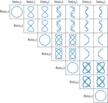
 αi
αi
 αproj
αproj αmanifold
 α1
α1 α3
α3 αproj,0
 α1
α1
 μn
μn
 α1,2
α1,2
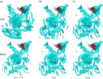


 δU
δU F(t)−F(t+T)

 βi
βi

 Open access

