


1 Introduction
The notion of a (planar) Stark–Zeeman system was introduced in [Reference Cieliebak, Frauenfelder and van Koert6]. It describes the motion of an electron in the plane attracted by a proton and subject to exterior electric and magnetic fields. Since Newton’s law of gravitation takes the same form as Coulomb’s law, we can also think of the electron as a light body gravitationally attracted by a proton as the heavy body. The Lorentz force from the magnetic field in this interpretation then corresponds to the Coriolis force. Many important systems from classical and celestial mechanics are Stark–Zeeman systems.
In a Stark–Zeeman system, the electron can collide with the proton, which causes singularities. Despite this, it is classically known that such singularities due to two-body collisions can be regularized. In [Reference Cieliebak, Frauenfelder and van Koert6], two invariants $\mathcal {J}_1$
and
$\mathcal {J}_1$
and $\mathcal {J}_2$
were defined for families of regularized periodic orbits in Stark–Zeeman systems as immersed planar curves without direct self-tangency, based on Arnold’s
$\mathcal {J}_2$
were defined for families of regularized periodic orbits in Stark–Zeeman systems as immersed planar curves without direct self-tangency, based on Arnold’s $J^+$
-invariant [Reference Arnold3], one for the unregularized system and another one for its Levi-Civita regularization.
$J^+$
-invariant [Reference Arnold3], one for the unregularized system and another one for its Levi-Civita regularization.
In this paper, we introduce the notion of a (planar) two-center Stark–Zeeman system. In this case, the electron is attracted by two protons and the energy is high enough that the electron can collide with both of them, but not so high that the electron may escape from being close enough to the protons. An example of a two-center Stark–Zeeman system is the restricted three-body problem for energies between the first and second critical values.
One of our motivations for defining $J^{+}$
-type invariants of planar periodic orbits is to gain a better understanding about whether periodic orbits in given Stark–Zeeman systems can be put in families of interpolating Stark–Zeeman systems. We shall introduce four
$J^{+}$
-type invariants of planar periodic orbits is to gain a better understanding about whether periodic orbits in given Stark–Zeeman systems can be put in families of interpolating Stark–Zeeman systems. We shall introduce four $J^+$
-like invariants for periodic orbits in a planar two-center Stark–Zeeman system. The generalization of the invariant
$J^+$
-like invariants for periodic orbits in a planar two-center Stark–Zeeman system. The generalization of the invariant $\mathcal {J}_1$
is straightforward. Since we have now two protons, we can consider the Levi-Civita regularization at either one of them. This leads to two generalizations of the invariant
$\mathcal {J}_1$
is straightforward. Since we have now two protons, we can consider the Levi-Civita regularization at either one of them. This leads to two generalizations of the invariant $\mathcal {J}_2$
which we will refer to as
$\mathcal {J}_2$
which we will refer to as $\mathcal {J}_E$
and
$\mathcal {J}_E$
and $\mathcal {J}_M$
. The reason for this terminology is that in the interpretation of the restricted three-body problem, one proton corresponds to the earth E and the other proton corresponds to the moon M. For two-center Stark–Zeeman systems, there is a regularization due to Birkhoff which simultaneously regularizes the collisions with both primaries, that is, with the Earth and the Moon. The Birkhoff regularization gives rise to a fourth pair of invariants, which we refer to as
$\mathcal {J}_M$
. The reason for this terminology is that in the interpretation of the restricted three-body problem, one proton corresponds to the earth E and the other proton corresponds to the moon M. For two-center Stark–Zeeman systems, there is a regularization due to Birkhoff which simultaneously regularizes the collisions with both primaries, that is, with the Earth and the Moon. The Birkhoff regularization gives rise to a fourth pair of invariants, which we refer to as $(\mathcal {J}_{E,M}, n)$
. We also analyze their relationships: depending on the parity of the winding numbers around E and M as well as their sums, sometimes one may express one of the invariants in terms of the others, while they are largely independent otherwise. The analysis is based on a construction called the interior connected sum, which can be thought of as the inversion of the connected sum construction of a homotopically non-trivial immersed loop with an exterior homotopically trivial loop.
$(\mathcal {J}_{E,M}, n)$
. We also analyze their relationships: depending on the parity of the winding numbers around E and M as well as their sums, sometimes one may express one of the invariants in terms of the others, while they are largely independent otherwise. The analysis is based on a construction called the interior connected sum, which can be thought of as the inversion of the connected sum construction of a homotopically non-trivial immersed loop with an exterior homotopically trivial loop.
2 Two-center Stark–Zeeman systems
Let $E, M \in \mathbb {R}^2 \cong \mathbb {C}$
be two distinct points which we refer to as the Earth and Moon. Suppose that
$E, M \in \mathbb {R}^2 \cong \mathbb {C}$
be two distinct points which we refer to as the Earth and Moon. Suppose that $\mu _E, \mu _M>0$
. Let
$\mu _E, \mu _M>0$
. Let
 $$ \begin{align*}V_E \colon \mathbb{R}^2 \setminus \{E\} \to \mathbb{R} \quad q \mapsto -\frac{\mu_E}{|q-E|}, \quad V_M \colon \mathbb{R}^2 \setminus \{M\} \to \mathbb{R}, \quad q \mapsto -\frac{\mu_M}{|q-M|}\end{align*} $$
be the gravitational potentials centered at the Earth and the Moon respectively. The parameters $\mu _E$
and
$\mu _E$
and $\mu _M$
thus represent the masses of the Earth and the Moon respectively. Alternatively, one may think of
$\mu _M$
thus represent the masses of the Earth and the Moon respectively. Alternatively, one may think of $V_E$
and
$V_E$
and $V_M$
as Coulomb potentials under which the interpretations of the parameters
$V_M$
as Coulomb potentials under which the interpretations of the parameters $\mu _E$
and
$\mu _E$
and $\mu _M$
become charges.
$\mu _M$
become charges.
Assume that $U_0 \subset \mathbb {R}^2$
is an open set containing E and M and
$U_0 \subset \mathbb {R}^2$
is an open set containing E and M and
 $$ \begin{align*}V_1 \colon U_0 \to \mathbb{R}\end{align*} $$
is a smooth function. Abbreviate
 $$ \begin{align*}U:=U_0 \setminus \{E,M\}\end{align*} $$
and define
 $$ \begin{align*}V:=V_E+V_M+V_1 \colon U \to \mathbb{R}.\end{align*} $$
The function $V_1$
can be interpreted as an additional potential which gives rise to additional position-dependent forces other than the gravitational forces of the Earth and the Moon.
$V_1$
can be interpreted as an additional potential which gives rise to additional position-dependent forces other than the gravitational forces of the Earth and the Moon.
Velocity-dependent forces, like the Lorentz force of a magnetic field or the Coriolis force, can be modeled by a twist in the standard symplectic form of the cotangent bundle of U: For a function $\mathcal {B} \in C^\infty (U_0,\mathbb {R})$
, let
$\mathcal {B} \in C^\infty (U_0,\mathbb {R})$
, let
 $$ \begin{align*}\sigma_{\mathcal{B}}=\mathcal{B} \, dq_1 \wedge dq_2 \in \Omega^2(U_0)\end{align*} $$
and define the twisted symplectic form
 $$ \begin{align*}\omega_{\mathcal{B}}=\sum_{i=1}^2 dp_i \wedge dq_i+\pi^* \sigma_{\mathcal{B}} \in \Omega^2(T^* U_0),\end{align*} $$
where $\pi \colon T^*U_0 \to U_0$
is the footpoint projection.
$\pi \colon T^*U_0 \to U_0$
is the footpoint projection.
We further choose a smooth Riemannian metric g on $TU_0$
. Let
$TU_0$
. Let $g^*$
be its dual metric on the cotangent bundle
$g^*$
be its dual metric on the cotangent bundle $T^{*} U_{0}$
of
$T^{*} U_{0}$
of $U_0$
. We define the Hamiltonian
$U_0$
. We define the Hamiltonian
 $$ \begin{align*}H=H_{V\!,g} \colon T^*U \to \mathbb{R}, \quad (q,p) \mapsto \tfrac{1}{2}\|p\|^2_{g^*_q}+V(q).\end{align*} $$
The dynamics of the Stark–Zeeman system is given by the flow of the Hamiltonian vector field $X^B_{V,g}$
implicitly defined by
$X^B_{V,g}$
implicitly defined by
 $$ \begin{align*}dH_{V\!,g}=\omega_{\mathcal{B}}(\cdot, X^{\mathcal{B}}_{V,g}).\end{align*} $$
As the Hamiltonian is autonomous (that is, independent of time), it is preserved under the flow of its Hamiltonian vector field (conservation of energy). We fix an energy value $c \in \mathbb {R}$
and consider a connected component
$c \in \mathbb {R}$
and consider a connected component
 $$ \begin{align*}\Sigma_c\subset H^{-1}(c)\end{align*} $$
of the energy hypersurface on level c. The Hill’s region is defined as its image under the footpoint projection
 $$ \begin{align*}\mathfrak{K}_c=\pi(\Sigma_c)\subset\{q \in U\mid V(q) \leq c\}.\end{align*} $$
We make the following two assumptions:
-
C(i) c is a regular value of H (or equivalently of V);
-
C(ii) $\mathfrak {K}_c\cup \{E,M\}$
is bounded and simply connected.
$\mathfrak {K}_c\cup \{E,M\}$
is bounded and simply connected.

3 Examples of planar 2-center Stark–Zeeman systems
In this section, we present a short list of classical planar 2-center Stark–Zeeman systems.
3.1 The planar circular restricted three-body problem
The first system which fits into this category is the planar circular restricted three-body problem in a rotating frame so that E and M are fixed at the positions $(-\mu _M,0)$
and
$(-\mu _M,0)$
and $(\mu _E,0)$
respectively. It is described by the Hamiltonian
$(\mu _E,0)$
respectively. It is described by the Hamiltonian
 $$ \begin{align*}H=\dfrac{|p|^{2}}{2} + V_{E} + V_{M} + V_{1}\end{align*} $$
with masses $\mu _{E},\mu _{M}>0$
, which we can normalize by setting
$\mu _{E},\mu _{M}>0$
, which we can normalize by setting $\mu _{E}+\mu _{M}=1$
. Here
$\mu _{E}+\mu _{M}=1$
. Here $V_{1}={|q|^{2}}/{2}$
is the potential which generates the centrifugal force around the center of mass of E and M, and the Coriolis force in the rotating frame is taken into account by the twisted symplectic form
$V_{1}={|q|^{2}}/{2}$
is the potential which generates the centrifugal force around the center of mass of E and M, and the Coriolis force in the rotating frame is taken into account by the twisted symplectic form
 $$ \begin{align*}\omega_{\mathcal{B}}=d (p_{1}-q_{2}) \wedge d q_{1} + d (p_{2} + q_{1}) \wedge d q_{2} = d p_{1} \wedge d q_{1} + d p_{2} \wedge d q_{2} + 2 d q_{1} \wedge d q_{2}.\end{align*} $$
There is vast literature on this problem which we will not even try to list. Let us just mention that when the energy of the system is below the first critical value, the Hill’s region has three connected components: one around the Earth; one around the Moon; and another one ‘around infinity’. When the energy c lies between the first and the second critical values (counted from below), the two bounded connected components around the Earth and the Moon merge into one bounded component $\Sigma _c$
of the energy hypersurface satisfying assumptions C(i) and C(ii). In this case, the corresponding Hill’s region is actually homeomorphic to the connected sum of two discs, each with a point removed. Above the second critical value, assumption C(ii) no longer holds.
$\Sigma _c$
of the energy hypersurface satisfying assumptions C(i) and C(ii). In this case, the corresponding Hill’s region is actually homeomorphic to the connected sum of two discs, each with a point removed. Above the second critical value, assumption C(ii) no longer holds.
3.2 The charged planar circular restricted three-body problem
The system is defined as in the planar circular restricted three-body problem, except that we no longer require $\mu _{E}, \mu _{M}$
to be positive. Instead, they can be either positive or negative. Such a system then models the motion of a charged particle in a magnetic field and the electric field generated by the two charges. Note that when
$\mu _{E}, \mu _{M}$
to be positive. Instead, they can be either positive or negative. Such a system then models the motion of a charged particle in a magnetic field and the electric field generated by the two charges. Note that when $\mu _{E}, \mu _{M}$
are not both positive, at least one of the force fields is repulsive. Therefore, such a system on a fixed regular energy hypersurface may not satisfy assumption C(ii).
$\mu _{E}, \mu _{M}$
are not both positive, at least one of the force fields is repulsive. Therefore, such a system on a fixed regular energy hypersurface may not satisfy assumption C(ii).
3.3 Euler’s two-center problem in the plane
Euler’s two-center problem describes a particle moving in the gravitational field generated by two fixed bodies (the centers). In the plane, this corresponds to the case where $\mu _{E}, \mu _{M}>0$
,
$\mu _{E}, \mu _{M}>0$
, $V_{1}\equiv 0$
, and
$V_{1}\equiv 0$
, and $\omega _{B}=\omega $
is the standard symplectic form. It was already known to Euler [Reference Euler8] that this problem is separable in suitable coordinates and thus integrable. Regular energy hypersurfaces above the first critical value with negative energy satisfy assumptions C(i), C(ii), while regular energy hypersurfaces with positive energy satisfy assumption C(i) but not C(ii).
$\omega _{B}=\omega $
is the standard symplectic form. It was already known to Euler [Reference Euler8] that this problem is separable in suitable coordinates and thus integrable. Regular energy hypersurfaces above the first critical value with negative energy satisfy assumptions C(i), C(ii), while regular energy hypersurfaces with positive energy satisfy assumption C(i) but not C(ii).
3.4 Lagrange’s modification of Euler’s two-center problem
The (planar) Lagrange problem is obtained from Euler’s two-center problem by adding a quadratic potential $V_{1}={|q|^{2}}/{2}$
at the midpoint of the two centers (which we may put at the origin). By the analysis of Lagrange [Reference Lagrange12], this system is also integrable.
$V_{1}={|q|^{2}}/{2}$
at the midpoint of the two centers (which we may put at the origin). By the analysis of Lagrange [Reference Lagrange12], this system is also integrable.
3.5 Euler’s problem and Lagrange’s modification on a sphere or pseudosphere
Euler’s two-center problem in the plane admits a generalization to the sphere and the pseudosphere, with the two-body potential replaced by $\mu \cot (\theta )$
and
$\mu \cot (\theta )$
and $\mu \, \mbox {coth}(\theta )$
, respectively. The system on the pseudosphere was defined and discussed in [Reference Killing10], see also [Reference Vozmischeva14]. On the sphere, the antipodal point of each center is again a center, with the strength constant
$\mu \, \mbox {coth}(\theta )$
, respectively. The system on the pseudosphere was defined and discussed in [Reference Killing10], see also [Reference Vozmischeva14]. On the sphere, the antipodal point of each center is again a center, with the strength constant $-\mu $
. There are thus overall four centers on the sphere, two attractive and two repulsive.
$-\mu $
. There are thus overall four centers on the sphere, two attractive and two repulsive.
A new interpretation of the integrability of Euler’s problem on the plane from the existence of Euler’s problem on the sphere via central projection was established by Albouy [Reference Albouy2]. He actually realized both problems as quasi-bi-Hamiltonian systems, that is, systems admitting two different Hamiltonian descriptions up to a time change. The projection of the spherical Hamiltonian then becomes a second conserved quantity of the planar system and vice versa. Moreover, in a gnomonic chart (given by the central projection from the center of the sphere) the spherical system takes the form of a Stark–Zeeman system with exactly the same potential as the planar system, just with a different kinetic energy. Lagrange’s modification has also been discussed within this approach [Reference Albouy2]. These systems in a gnomonic chart thus provide examples of two-center Stark–Zeeman systems with non-standard kinetic parts. Note that if instead we use a chart defined by stereographic projection, then in this chart, the metric is conformal to the Euclidean metric and the singularities of these systems are asymptotically of Newtonian type, which allows us to treat these systems as examples of two-center Stark–Zeeman systems to which all the discussion below will apply.
4 Partial and simultaneous regularizations of double collisions in planar 2-center Stark–Zeeman systems
For a (planar) two-center Stark–Zeeman system, energy hypersurfaces which project to bounded Hill’s regions are still non-compact due to the presence of collisions with the primaries. Nevertheless, we know that such collisions can be regularized, either individually or simultaneously. In this section, we shall present adaptations of the Levi-Civita regularization for regularizing only one collision, and Birkhoff’s simultaneous regularization of both collisions. There exist also other regularizations, but the Levi-Civita and Birkhoff regularizations are most suitable for our investigation of closed orbits in these systems via invariants of immersed planar loops.
4.1 Partial Levi-Civita regularizations
We recall the Levi-Civita regularization of the planar Kepler problem. After normalization of the masses, the Hamiltonian of the system is given by
 $$ \begin{align*}H(q,p)=\dfrac{|p|^{2}}{2}-\dfrac{1}{|q|}\end{align*} $$
for $(q,p) \in \mathbb {C}\setminus \{0\} \times \mathbb {C}$
. To regularize the singularity at
$(q,p) \in \mathbb {C}\setminus \{0\} \times \mathbb {C}$
. To regularize the singularity at $q=0$
, we fix an energy
$q=0$
, we fix an energy $c=-f<0$
and consider the Hamiltonian flow on
$c=-f<0$
and consider the Hamiltonian flow on $\Sigma _c=H^{-1}(c)$
. We change time on this energy hypersurface by rescaling the Hamiltonian to
$\Sigma _c=H^{-1}(c)$
. We change time on this energy hypersurface by rescaling the Hamiltonian to
 $$ \begin{align*}\widetilde{H}(q,p):=|q| (H(q,p)-c)=\dfrac{|q||p|^{2}}{2} +f |q| -1.\end{align*} $$
We now consider the complex square mapping
 $$ \begin{align*}L:\mathbb{C}\setminus\{0\} \to \mathbb{C}\setminus\{0\}, \quad z \mapsto z^{2}.\end{align*} $$
Its cotangent lift is the symplectomorphism
 $$ \begin{align*}T^*L: \mathbb{C} \setminus \{0\} \times \mathbb{C} \to \mathbb{C} \setminus \{0\} \times \mathbb{C}, \quad (z, w) \mapsto \bigg(z^{2}, \dfrac{w}{2 \bar{z}}\bigg).\end{align*} $$
The regularized Hamiltonian K is defined by pulling back $\widetilde {H}$
under
$\widetilde {H}$
under $T^*L$
,
$T^*L$
,
 $$ \begin{align*}K(z,w):=\widetilde H\circ T^*L (z,w)=\dfrac{|w|^{2}}{8} +f |z|^{2} -1.\end{align*} $$
The collision locus $\{q=0\}$
in the closure of
$\{q=0\}$
in the closure of $\Sigma _c$
is transformed to the set
$\Sigma _c$
is transformed to the set $\{z=0\}$
in the regular energy hypersurface
$\{z=0\}$
in the regular energy hypersurface $\{K=0\}$
, which is no longer singular. These collisions are thus regularized.
$\{K=0\}$
, which is no longer singular. These collisions are thus regularized.
The Levi-Civita regularization extends to smoothly perturbed Kepler problems, in particular to all one-center Stark–Zeeman systems. It applies also to two-center Stark–Zeeman systems when we want to regularize only double collisions at either E or M. We shall call these the partial regularizations with respect to E and M respectively. The other singularity remains non-regularized and, since the map L is two-to-one, the non-regularized singularity doubles to two singularities in the partially regularized system. The two new singularities are still asymptotically of the type of a Newtonian-type singularity: To see this, assume that the non-regularized singularity is located at $q=1$
and the potential is of the form
$q=1$
and the potential is of the form $-{1}/{|q-1|}$
. It contributes to the regularized system an additional term
$-{1}/{|q-1|}$
. It contributes to the regularized system an additional term $-{|z|^{2}}/{|z^{2}-1|}=-{|z|^{2}}/{|z+1| |z-1|}$
, so the two new singularities are located at
$-{|z|^{2}}/{|z^{2}-1|}=-{|z|^{2}}/{|z+1| |z-1|}$
, so the two new singularities are located at $z=\pm 1$
and are of Newtonian type. We remark that this partial regularization procedure can thus be iterated, which is however not what we are going to investigate here. In addition, we remark that the regularization procedure naturally extends to the case where the kinetic part of the Hamiltonian is given by a metric conformal to the standard Euclidean metric.
$z=\pm 1$
and are of Newtonian type. We remark that this partial regularization procedure can thus be iterated, which is however not what we are going to investigate here. In addition, we remark that the regularization procedure naturally extends to the case where the kinetic part of the Hamiltonian is given by a metric conformal to the standard Euclidean metric.
4.2 Waldvogel’s interpretation of Birkhoff’s regularization
We now present a regularization due to Birkhoff [Reference Birkhoff5] of planar two-center Stark–Zeeman systems. By normalization, we put E and M at $-1$
and
$-1$
and $1$
respectively.
$1$
respectively.
In [Reference Waldvogel15], Waldvogel remarked that the complex square mapping $L(z)=z^{2}$
used in the Levi-Civita regularization extends to a conformal mapping from the Riemann sphere
$L(z)=z^{2}$
used in the Levi-Civita regularization extends to a conformal mapping from the Riemann sphere $\mathbb {C} \cup \{\infty \}$
to itself fixing
$\mathbb {C} \cup \{\infty \}$
to itself fixing $0$
and
$0$
and $\infty $
which, in Waldvogel’s words [Reference Waldvogel15], also ‘regularizes’ a ‘similar singularity’ at infinity. With this in mind, Waldvogel interpreted the Birkhoff regularization mapping
$\infty $
which, in Waldvogel’s words [Reference Waldvogel15], also ‘regularizes’ a ‘similar singularity’ at infinity. With this in mind, Waldvogel interpreted the Birkhoff regularization mapping
 $$ \begin{align} B:\mathbb{C}^*=\mathbb{C}\setminus\{0\}\to\mathbb{C},\quad B(z)=\tfrac{1}{2} (z + 1/z) \end{align} $$
as the conjugation $B = T^{-1} \circ L \circ T$
of the complex square mapping L by the Möbius transformation
$B = T^{-1} \circ L \circ T$
of the complex square mapping L by the Möbius transformation
 $$ \begin{align*}T(z)=1-\dfrac{2}{1-z}=T^{-1}(z) \end{align*} $$
sending $-1$
to
$-1$
to $0$
and
$0$
and $+1$
to
$+1$
to $\infty $
. Thus, B extends to a branched double cover
$\infty $
. Thus, B extends to a branched double cover $\mathbb {C}\cup \{\infty \}\to \mathbb {C}\cup \{\infty \}$
, sending
$\mathbb {C}\cup \{\infty \}\to \mathbb {C}\cup \{\infty \}$
, sending $0$
and
$0$
and $\infty $
to
$\infty $
to $\infty $
, with two branch points at
$\infty $
, with two branch points at $\pm 1$
of values
$\pm 1$
of values $\pm 1$
. See Figure 1.
$\pm 1$
. See Figure 1.
Birkhoff regularization.

The cotangent lift of B is given by
 $$ \begin{align} T^*B:T^*\mathbb{C}^*\to T^*\mathbb{C},\quad (z,w)\mapsto (q,p)=\bigg(\frac{z^2+1}{2z},\dfrac{2 \bar{z}^{2}}{\bar{z}^{2}-1} w\bigg). \end{align} $$
We will now explain the regularization of two-center Stark–Zeeman systems with this method, with Euler’s two-center problem as the first example.
4.3 Birkhoff simultaneous regularization of Euler’s two-center problem
In complex variables $(q,p) \in \mathbb {C}\setminus \{0, 1\} \times \mathbb {C}$
, the Hamiltonian of the two-center problem is
$(q,p) \in \mathbb {C}\setminus \{0, 1\} \times \mathbb {C}$
, the Hamiltonian of the two-center problem is
 $$ \begin{align*}H=\dfrac{|p|^{2}}{2}-\dfrac{\mu}{|q-1|}-\dfrac{1-\mu}{|q+1|}.\end{align*} $$
After fixing a negative energy $c=-f$
and rescaling time on this energy surface, we get that the slowed-down flow on this energy surface is governed by the following Hamiltonian restricted to the zero-energy level:
$c=-f$
and rescaling time on this energy surface, we get that the slowed-down flow on this energy surface is governed by the following Hamiltonian restricted to the zero-energy level:
 $$ \begin{align*}|q-1|\, |q+1| (H+f)&=\dfrac{|q-1|\, |q+1||p|^{2}}{2}-\mu |q+1| -(1-\mu)|q-1|\\ & \quad + f |q-1|\, |q+1|.\end{align*} $$
Substituting $(q,p)$
by
$(q,p)$
by $(z,w)$
via equation (2) and further dividing by
$(z,w)$
via equation (2) and further dividing by $|z|^{2}$
results in the Hamiltonian
$|z|^{2}$
results in the Hamiltonian
 $$ \begin{align*}K(z,w)=\dfrac{|w|^{2}}{2} - \dfrac{ \mu |z+1|^{2}}{2 |z|^{3}} - \dfrac{(1-\mu) |z-1|^{2}}{2 |z|^{3}}+f\dfrac{|z-1|^{2} |z+1|^{2}}{4 |z|^{4}}.\end{align*} $$
We observe that this system is no longer singular at the transformed collision sets $\{z=\pm 1\}$
in
$\{z=\pm 1\}$
in $\{K=0\}$
. The Hamiltonian K has a singularity at
$\{K=0\}$
. The Hamiltonian K has a singularity at $z=0$
, which however corresponds to energy
$z=0$
, which however corresponds to energy $K=\infty $
and therefore does not lie on the energy hypersurface
$K=\infty $
and therefore does not lie on the energy hypersurface $\{K=0\}$
. The regularized Hill’s region, i.e. the footpoint projection of the energy hypersurface
$\{K=0\}$
. The regularized Hill’s region, i.e. the footpoint projection of the energy hypersurface $\{K=0\}$
, is the subset in
$\{K=0\}$
, is the subset in $\mathbb {C}$
described in polar coordinates
$\mathbb {C}$
described in polar coordinates $z=r e^{i \theta }$
by the inequality
$z=r e^{i \theta }$
by the inequality
 $$ \begin{align*}g_\theta(r):=2 r^{3} + 2 r -4 (1-2 \mu) r^{2} \cos \theta -f (r^{2} -2 r \cos \theta +1) (r^{2} +2 r \cos \theta +1)\geq0.\end{align*} $$
Proposition 4.1. For any $\mu \in (0, 1/2]$
there exists
$\mu \in (0, 1/2]$
there exists $f_{\mu }>0$
such that for all values
$f_{\mu }>0$
such that for all values $0<f<f_{\mu }$
, the regularized Hill’s region of the two-center problem at energy
$0<f<f_{\mu }$
, the regularized Hill’s region of the two-center problem at energy $-f$
is an annulus in
$-f$
is an annulus in $\mathbb {C}$
bounded by the boundaries of two star-shaped regions with respect to the origin.
$\mathbb {C}$
bounded by the boundaries of two star-shaped regions with respect to the origin.
Proof. It suffices to show that the quartic equation $g_\theta (r)=0$
has exactly two positive real roots for any
$g_\theta (r)=0$
has exactly two positive real roots for any $\theta $
. Let
$\theta $
. Let $\Delta _\theta $
be the discriminant of the quartic polynomial
$\Delta _\theta $
be the discriminant of the quartic polynomial $g_\theta (r)$
; an explicit formula of the discriminant in terms of the coefficients can be found at https://en.wikipedia.org/wiki/Discriminant#Degree_4. A calculation by Maple yields the factorization
$g_\theta (r)$
; an explicit formula of the discriminant in terms of the coefficients can be found at https://en.wikipedia.org/wiki/Discriminant#Degree_4. A calculation by Maple yields the factorization
 $$ \begin{align*}\Delta_\theta=4096 f_{1}^{2} f_{2} f_{3},\end{align*} $$
where
 $$ \begin{align*}f_{1}=1/4+f^2 \cos^{2} \theta+f (-1+2 \mu) \cos \theta,\end{align*} $$
 $$ \begin{align*}f_{2}=f \cos^{2} \theta+(-1+2 \mu) \cos \theta-f-1,\end{align*} $$
 $$ \begin{align*}f_{3}=f \cos^{2} \theta+(-1+2 \mu) \cos \theta-f+1.\end{align*} $$
We see that the discriminant is negative once $\mu \in (0,1/2]$
is fixed and f is chosen small enough. This implies that there exist exactly two real roots for
$\mu \in (0,1/2]$
is fixed and f is chosen small enough. This implies that there exist exactly two real roots for $g_\theta (r)$
and these real roots are distinct.
$g_\theta (r)$
and these real roots are distinct.
To see that both of these real roots are positive, note that $\lim _{r \to +\infty } g_\theta (r)<0$
and
$\lim _{r \to +\infty } g_\theta (r)<0$
and $g_\theta (0)<0$
. However, a short calculation yields
$g_\theta (0)<0$
. However, a short calculation yields $g_\theta (1)>0$
for f sufficiently small. Alternatively, we can use connectedness and non-contractibility of the regularized Hill’s region asserted in Proposition 4.2 below to conclude that there must exist some
$g_\theta (1)>0$
for f sufficiently small. Alternatively, we can use connectedness and non-contractibility of the regularized Hill’s region asserted in Proposition 4.2 below to conclude that there must exist some $r>0$
for which
$r>0$
for which $g_\theta (r)>0$
. Either way, we conclude that for any
$g_\theta (r)>0$
. Either way, we conclude that for any $\theta $
, the polynomial
$\theta $
, the polynomial $g_\theta (r)$
has exactly two positive roots.
$g_\theta (r)$
has exactly two positive roots.
4.4 Birkhoff regularization of two-center Stark–Zeeman systems
Consider now a general two-center Stark–Zeeman system as in §2 such that the metric g used in the kinetic energy is conformal to the standard metric. Then replacing p by $2\bar z^2w/(\bar z^2-1)$
yields
$2\bar z^2w/(\bar z^2-1)$
yields $\|p\|_{g^*_q} = 2|z|^2\|w\|_{g^*_q}/|z^2-1|$
and the computation of the previous section goes through. Thus for a regular value c satisfying conditions C(i) and C(ii), the level set
$\|p\|_{g^*_q} = 2|z|^2\|w\|_{g^*_q}/|z^2-1|$
and the computation of the previous section goes through. Thus for a regular value c satisfying conditions C(i) and C(ii), the level set $\Sigma _c\subset H^{-1}(c)$
pulls back under
$\Sigma _c\subset H^{-1}(c)$
pulls back under $T^*B$
to
$T^*B$
to $\Sigma _c^B\subset K^{-1}(0)$
for the rescaled pullback Hamiltonian
$\Sigma _c^B\subset K^{-1}(0)$
for the rescaled pullback Hamiltonian
 $$ \begin{align*} K(z,w) = \dfrac{\|w\|_{g^*_q}^{2}}{2} - \dfrac{ \mu_M |z+1|^{2}}{2 |z|^{3}} - \dfrac{\mu_E |z-1|^{2}}{2 |z|^{3}}+\dfrac{(V_1(q)-c)|z-1|^{2} |z+1|^{2}}{4 |z|^{4}}, \end{align*} $$
where q needs to be replaced by $(z^2+1)/2z$
. The singular point
$(z^2+1)/2z$
. The singular point $z=0$
corresponds to
$z=0$
corresponds to $q=\infty $
which lies outside the closure
$q=\infty $
which lies outside the closure $\bar {\mathfrak {K}}_c$
of the bounded Hill’s region. So the hypersurface
$\bar {\mathfrak {K}}_c$
of the bounded Hill’s region. So the hypersurface $\Sigma _c^B$
is regular and compact, and we call it the Birkhoff regularization of
$\Sigma _c^B$
is regular and compact, and we call it the Birkhoff regularization of $\Sigma _c$
. Note that the standard symplectic form twisted by a magnetic field
$\Sigma _c$
. Note that the standard symplectic form twisted by a magnetic field $\sigma $
pulls back under
$\sigma $
pulls back under $T^*B$
to the standard symplectic form twisted by the pullback magnetic field
$T^*B$
to the standard symplectic form twisted by the pullback magnetic field $B^*\sigma $
.
$B^*\sigma $
.
The footpoint projection of the Birkhoff regularized energy hypersurface $\Sigma _c^B$
is the preimage
$\Sigma _c^B$
is the preimage $B^{-1}(\bar {\mathfrak {K}}_c)$
under the map B from equation (1). Recall that we have normalized the positions of the Earth and Moon to
$B^{-1}(\bar {\mathfrak {K}}_c)$
under the map B from equation (1). Recall that we have normalized the positions of the Earth and Moon to $E=-1$
and
$E=-1$
and $M=+1$
; we denote the winding numbers around these points by
$M=+1$
; we denote the winding numbers around these points by $w_E$
and
$w_E$
and $w_M$
respectively. Then Proposition 4.1 generalizes to the following proposition.
$w_M$
respectively. Then Proposition 4.1 generalizes to the following proposition.
Proposition 4.2.
-
(a) The regularized Hill’s region
$B^{-1}(\bar {\mathfrak {K}}_c)\subset \mathbb {C}^*$
is an embedded annulus enclosing the origin. -
(b) The preimage
$B^{-1}(K)\subset \mathbb {C}^*$
of a closed curve
$K\subset \mathbb {C} \setminus \{E, M\}$
is connected if
$w_{E} (K) + w_{M} (K)$
is odd, and has two connected components if
$w_{E} (K) + w_{M} (K)$
is even.


Proof. Recall that map $B:\mathbb {C}^*\to \mathbb {C}$
from equation (1) is a branched double cover with two branch points at
$B:\mathbb {C}^*\to \mathbb {C}$
from equation (1) is a branched double cover with two branch points at $\pm 1$
of values
$\pm 1$
of values $\pm 1$
. So each loop
$\pm 1$
. So each loop $K\subset \mathbb {C}\setminus \{-1,1\}$
lifts to a path in
$K\subset \mathbb {C}\setminus \{-1,1\}$
lifts to a path in $\mathbb {C}^*$
which closes up if and only if
$\mathbb {C}^*$
which closes up if and only if $w_E(K)+w_M(K)$
is even. Part (b) immediately follows from this. For part (a), note that B maps the unit circle onto the interval
$w_E(K)+w_M(K)$
is even. Part (b) immediately follows from this. For part (a), note that B maps the unit circle onto the interval $[-1,1]$
, see Figure 1. Hence the preimage of an embedded circle
$[-1,1]$
, see Figure 1. Hence the preimage of an embedded circle $K\subset \mathbb {C}$
winding once around
$K\subset \mathbb {C}$
winding once around $-1$
and
$-1$
and $+1$
consists of two disjoint embedded circles in
$+1$
consists of two disjoint embedded circles in $\mathbb {C}^*$
isotopic to the unit circle, and the preimage of any embedded disk
$\mathbb {C}^*$
isotopic to the unit circle, and the preimage of any embedded disk $D\subset \mathbb {C}$
containing
$D\subset \mathbb {C}$
containing $-1$
and
$-1$
and $+1$
(such as
$+1$
(such as $D=\bar {\mathfrak {K}}_c$
) is an embedded annulus in
$D=\bar {\mathfrak {K}}_c$
) is an embedded annulus in $\mathbb {C}^*$
enclosing the origin.
$\mathbb {C}^*$
enclosing the origin.
Érdi [Reference Érdi7] explains a way to deduce many other (known) regularizations of two-center Stark–Zeeman systems (Le Maitre, Thiele–Burrau, Brouke, Wintner,…) by composing the Birkhoff regularization with additional smooth transformations. The Birkhoff regularization is therefore a common basis to all these other regularizations.
4.5 Birkhoff versus Moser regularization
We continue to use the notation from the previous subsection. Recall that the Birkhoff map $B(z)=(z+1/z)/2$
defines a double cover
$B(z)=(z+1/z)/2$
defines a double cover $B:\mathbb {C}^*\to \mathbb {C}$
branched at
$B:\mathbb {C}^*\to \mathbb {C}$
branched at $E=-1$
and
$E=-1$
and $M=+1$
. It is invariant under the inversion
$M=+1$
. It is invariant under the inversion $\phi (z)=1/z$
which interchanges the two sheets of the cover. Hence the cotangent lift
$\phi (z)=1/z$
which interchanges the two sheets of the cover. Hence the cotangent lift $T^*B:T^*\mathbb {C}^*\to T^*\mathbb {C}$
of B is invariant under the cotangent lift of
$T^*B:T^*\mathbb {C}^*\to T^*\mathbb {C}$
of B is invariant under the cotangent lift of $\phi $
,
$\phi $
,
 $$ \begin{align*}\Phi:=T^*\phi:T^*\mathbb{C}^*\to T^*\mathbb{C}^*,\quad (z,w)\mapsto (z^{-1},-\bar z^2w). \end{align*} $$
By its construction as a compactification of $(T^*B)^{-1}(\Sigma _c)$
, the Birkhoff regularized hypersurface
$(T^*B)^{-1}(\Sigma _c)$
, the Birkhoff regularized hypersurface $\Sigma _c^B$
is invariant under
$\Sigma _c^B$
is invariant under $\Phi $
. (In fact, a direct computation shows
$\Phi $
. (In fact, a direct computation shows $K\circ \Phi (z,w)=|z|^4K(z,w)$
for the Hamiltonian K of the previous subsection.) Since the fixed points
$K\circ \Phi (z,w)=|z|^4K(z,w)$
for the Hamiltonian K of the previous subsection.) Since the fixed points $(\pm 1,0)$
of
$(\pm 1,0)$
of $\Phi $
do not belong to
$\Phi $
do not belong to $K^{-1}(0)$
, the action of
$K^{-1}(0)$
, the action of $\Phi $
on
$\Phi $
on $\Sigma _c^B$
is free. So we obtain a quotient manifold
$\Sigma _c^B$
is free. So we obtain a quotient manifold $\Sigma _c^M$
and a two-to-one covering
$\Sigma _c^M$
and a two-to-one covering
 $$ \begin{align} P:\Sigma_c^B\to \Sigma_c^M. \end{align} $$
By construction, $\Sigma _c^M$
is a smooth compactification of the energy hypersurface
$\Sigma _c^M$
is a smooth compactification of the energy hypersurface $\Sigma _c$
and we call it the simultaneous Moser regularization at E and M. Note that near each branch point
$\Sigma _c$
and we call it the simultaneous Moser regularization at E and M. Note that near each branch point $E,M$
, the Birkhoff map looks like the Levi-Civita map around that point, so the two-to-one covering in equation (3) is consistent with the two-to-one covering between the Levi-Civita and Moser regularizations of one-center Stark–Zeeman systems used in [Reference Cieliebak, Frauenfelder and van Koert6].
$E,M$
, the Birkhoff map looks like the Levi-Civita map around that point, so the two-to-one covering in equation (3) is consistent with the two-to-one covering between the Levi-Civita and Moser regularizations of one-center Stark–Zeeman systems used in [Reference Cieliebak, Frauenfelder and van Koert6].
The following proposition describes the topology of the covering in equation (3).
Proposition 4.3.
-
(a) There exist diffeomorphisms
such that the first diffeomorphism conjugates the involution
$$ \begin{align*}\Sigma_c^B\cong S^1\times S^2\quad\text{and}\quad \Sigma_c^M\cong\mathbb{R} P^3\#\mathbb{R} P^3 \end{align*} $$
$\Phi :\Sigma _c^B\to \Sigma _c^B$
to the map
$S^1\times S^2\to S^1\times S^2$
,
$(\theta ,u)\mapsto (-\theta ,-u)$
(writing
$S^1=\mathbb {R}/2\pi \mathbb {Z}$
).
-
(b) The induced map between fundamental groups is given by
where e and m are represented by lifts of small loops around E and M, respectively.
$$ \begin{align*}P_*:\pi_1(\Sigma_c^B)=\mathbb{Z}\to \pi_1(\Sigma_c^M)=\mathbb{Z}_2*\mathbb{Z}_2,\quad n\mapsto(em)^n, \end{align*} $$
-
(c) The free homotopy classes of loops in
$\Sigma _c^M\cong \mathbb {R} P^3\#\mathbb {R} P^3$
correspond to the conjugacy classes
$[e]$
,
$[m]$
, and
$[(em)^n]$
for
$n\in \mathbb {N}_0$
in
$\pi _1(\mathbb {R} P^3\#\mathbb {R} P^3)=\mathbb {Z}_2*\mathbb {Z}_2$
.


Proof. (a) Recall that the closure of the Hill’s region $\mathfrak {K}_c$
is a closed disk D containing
$\mathfrak {K}_c$
is a closed disk D containing $E=-1$
and
$E=-1$
and $M=1$
, and its preimage
$M=1$
, and its preimage $A:=B^{-1}(D)$
is a closed annulus enclosing the origin, see Figure 1. After deforming the Stark–Zeeman system (which does not affect the assertions of the proposition), we may assume that
$A:=B^{-1}(D)$
is a closed annulus enclosing the origin, see Figure 1. After deforming the Stark–Zeeman system (which does not affect the assertions of the proposition), we may assume that
 $$ \begin{align*}A = \{z\in\mathbb{C}\mid e^{-1}\leq|z|\leq e\} = \{z=e^{\rho+i\theta}\in\mathbb{C}\mid -1\leq\rho\leq 1\}. \end{align*} $$
We use $(\rho ,\theta )\in [-1,1]\times \mathbb {R}/2\pi \mathbb {Z}$
as coordinates on A, in which the inversion
$(\rho ,\theta )\in [-1,1]\times \mathbb {R}/2\pi \mathbb {Z}$
as coordinates on A, in which the inversion $\phi (z)=z^{-1}$
sends
$\phi (z)=z^{-1}$
sends $(\rho , \theta )$
to
$(\rho , \theta )$
to $(-\rho , -\theta )$
. The footpoint projection
$(-\rho , -\theta )$
. The footpoint projection $\pi :\Sigma _c^B\to A$
defines a circle bundle over the interior of A whose fiber circles collapse to points over the boundary
$\pi :\Sigma _c^B\to A$
defines a circle bundle over the interior of A whose fiber circles collapse to points over the boundary $\partial A$
(the zero velocity curves). Thus for each fixed angle
$\partial A$
(the zero velocity curves). Thus for each fixed angle $\theta $
, the preimage
$\theta $
, the preimage $\pi ^{-1}([-1,1]\times \{\theta \})$
is a
$\pi ^{-1}([-1,1]\times \{\theta \})$
is a $2$
-sphere, which gives the first diffeomorphism
$2$
-sphere, which gives the first diffeomorphism $\Sigma _c^B\cong S^1\times S^2$
. Note that coordinates on
$\Sigma _c^B\cong S^1\times S^2$
. Note that coordinates on $S^1\times S^2$
are given by
$S^1\times S^2$
are given by $(\theta ,u)$
, where
$(\theta ,u)$
, where $\theta \in \mathbb {R}/2\pi \mathbb {Z}$
and
$\theta \in \mathbb {R}/2\pi \mathbb {Z}$
and $u=(\rho ,w)\in [-1,1]\times \mathbb {C}$
with
$u=(\rho ,w)\in [-1,1]\times \mathbb {C}$
with $\rho ^2+|w|^2=1$
. Hence in these coordinates, the map
$\rho ^2+|w|^2=1$
. Hence in these coordinates, the map $\Phi (z,w)=(z^{-1},-\bar z^2w)$
takes (after rescaling w) the form
$\Phi (z,w)=(z^{-1},-\bar z^2w)$
takes (after rescaling w) the form
 $$ \begin{align*}\Phi:S^1\times S^2\to S^1\times S^2,\quad (\theta,(\rho,w))\mapsto(-\theta,(-\rho,-e^{-2i\theta}w)). \end{align*} $$
Conjugating $\Phi $
by the diffeomorphism
$\Phi $
by the diffeomorphism
 $$ \begin{align*}\Gamma:S^1\times S^2\to S^1\times S^2,\quad (\theta,(\rho,w))\mapsto(\theta,(\rho,e^{-i\theta}w)) \end{align*} $$
yields the desired map
 $$ \begin{align*}\Gamma\Phi\Gamma^{-1}(\theta,(\rho,w)) = \Gamma\Phi(\theta,(\rho,e^{i\theta}w)) = \Gamma(-\theta,(-\rho,-e^{-i\theta}w)) = (-\theta,(-\rho,-w)). \end{align*} $$
For the second diffeomorphism, we view D as the boundary connected sum of two disks around E and M. Then $\Sigma _c^M$
is the connected sum
$\Sigma _c^M$
is the connected sum $\Sigma _E^M\#\Sigma _M^M$
of two Moser regularized energy hypersurfaces in one-center Stark–Zeeman systems, each being diffeomorphic to
$\Sigma _E^M\#\Sigma _M^M$
of two Moser regularized energy hypersurfaces in one-center Stark–Zeeman systems, each being diffeomorphic to $\mathbb {R} P^3$
as shown e.g. in [Reference Cieliebak, Frauenfelder and van Koert6]. Alternatively, consider small closed disks
$\mathbb {R} P^3$
as shown e.g. in [Reference Cieliebak, Frauenfelder and van Koert6]. Alternatively, consider small closed disks $D_E,D_M\subset \mathrm {Int}\,D$
around
$D_E,D_M\subset \mathrm {Int}\,D$
around $E,M$
. Then
$E,M$
. Then $\pi ^{-1}(D_E),\pi ^{-1}(D_M)\subset \Sigma _c^M$
are solid tori and
$\pi ^{-1}(D_E),\pi ^{-1}(D_M)\subset \Sigma _c^M$
are solid tori and $\Sigma _c^M\setminus (\pi ^{-1}(D_E)\amalg \pi ^{-1}(D_M){)}$
is diffeomorphic to
$\Sigma _c^M\setminus (\pi ^{-1}(D_E)\amalg \pi ^{-1}(D_M){)}$
is diffeomorphic to $S^3\setminus (T_E\amalg T_M)$
for unlinked and unknotted solid tori
$S^3\setminus (T_E\amalg T_M)$
for unlinked and unknotted solid tori $T_E,T_M\subset S^3$
. The local description of the Moser regularization near E shows that to recover
$T_E,T_M\subset S^3$
. The local description of the Moser regularization near E shows that to recover $\Sigma _c^M$
, both
$\Sigma _c^M$
, both $T_E$
and
$T_E$
and $T_M$
are glued in along their boundary by a diffeomorphism mapping the meridian to twice the meridian plus the longitude. Thus,
$T_M$
are glued in along their boundary by a diffeomorphism mapping the meridian to twice the meridian plus the longitude. Thus, $\Sigma _c^M$
is the
$\Sigma _c^M$
is the $2/1$
-Dehn surgery of
$2/1$
-Dehn surgery of $S^3$
along two unlinked unknots (see e.g. [Reference Gordon9]), which equals
$S^3$
along two unlinked unknots (see e.g. [Reference Gordon9]), which equals $\mathbb {R} P^3\#\mathbb {R} P^3$
.
$\mathbb {R} P^3\#\mathbb {R} P^3$
.
(b) By the description of the diffeomorphism $\Sigma _c^B\cong S^1\times S^2$
in item (a), the outer boundary of A represents a generator of
$\Sigma _c^B\cong S^1\times S^2$
in item (a), the outer boundary of A represents a generator of $S^1$
. Since it is mapped under B onto
$S^1$
. Since it is mapped under B onto $\partial D$
, and B lifts to P, this shows that
$\partial D$
, and B lifts to P, this shows that $P_*$
maps a generator of
$P_*$
maps a generator of $\pi _1(\Sigma _c^B)$
onto
$\pi _1(\Sigma _c^B)$
onto $em$
.
$em$
.
(c) Note that each element in $\mathbb {Z}_2*\mathbb {Z}_2$
is of the form
$\mathbb {Z}_2*\mathbb {Z}_2$
is of the form $a_n=(em)^n$
,
$a_n=(em)^n$
, $b_n=m(em)^n$
, or
$b_n=m(em)^n$
, or $c_n=(em^n)e$
for some
$c_n=(em^n)e$
for some $n\in \mathbb {N}_0$
. Since
$n\in \mathbb {N}_0$
. Since $mb_nm^{-1}=c_{n-1}$
and
$mb_nm^{-1}=c_{n-1}$
and $ec_ne^{-1}=b_{n-1}$
, all the elements
$ec_ne^{-1}=b_{n-1}$
, all the elements $b_n,c_n$
are conjugated to either e or m.
$b_n,c_n$
are conjugated to either e or m.
Remark 4.4. Proposition 4.3 implies that the quotient of $S^1\times S^2$
under the fixed point free involution
$S^1\times S^2$
under the fixed point free involution $\Phi (\theta ,u)=(-\theta ,-u)$
is diffeomorphic to
$\Phi (\theta ,u)=(-\theta ,-u)$
is diffeomorphic to $\mathbb {R} P^3\#\mathbb {R} P^3$
. The geometry of the Birkhoff map leads to the following direct description of this diffeomorphism. Write
$\mathbb {R} P^3\#\mathbb {R} P^3$
. The geometry of the Birkhoff map leads to the following direct description of this diffeomorphism. Write
 $$ \begin{align*}S^1=\mathbb{R}/2\pi\mathbb{Z} = I_0\cup I_2\cup I_3\cup I_4 \end{align*} $$
as the union of the four intervals
 $$ \begin{align*}I_0= \bigg[-\frac{\pi}{4},\frac{\pi}{4}\bigg],\quad I_1=\bigg[\frac{\pi}{4},\frac{3\pi}{4}\bigg],\quad I_2= \bigg[\frac{3\pi}{4},\frac{5\pi}{4}\bigg],\quad I_3= \bigg[\frac{5\pi}{4},\frac{7\pi}{4}\bigg] \end{align*} $$
glued at their endpoints. See Figure 2. Note that the map $\theta \mapsto -\theta $
preserves
$\theta \mapsto -\theta $
preserves $I_0$
,
$I_0$
, $I_2$
and interchanges
$I_2$
and interchanges $I_1$
with
$I_1$
with $I_3$
. Now we perform two
$I_3$
. Now we perform two $2$
-surgeries on
$2$
-surgeries on $S^1\times S^2$
along the spheres
$S^1\times S^2$
along the spheres $\pi /2\times S^2$
and
$\pi /2\times S^2$
and $3\pi /2\times S^2$
, whose result can be explicitly written as (with the obvious gluings along the boundaries)
$3\pi /2\times S^2$
, whose result can be explicitly written as (with the obvious gluings along the boundaries)
 $$ \begin{align*} N :&= (S^1\times S^2\setminus(\mathring{I_1}\cup\mathring{I_3})\times S^2)\cup(\partial I_1\cup\partial I_3)\times B^3 \cr &= (I_0\times S^2\cup\partial I_0\times B^3)\amalg (I_2\times S^2\cup\partial I_2\times B^3). \end{align*} $$
The circle and the intervals.

Here $(I_0\times S^2\cup \partial I_0\times B^3)\cong S^3$
and the involution
$(I_0\times S^2\cup \partial I_0\times B^3)\cong S^3$
and the involution $\Phi $
extends over
$\Phi $
extends over $\partial I_0\times B^3$
via
$\partial I_0\times B^3$
via $\Phi (\pm \pi /4,u)=(\mp \pi /4,-u)$
. This gives the antipodal map on
$\Phi (\pm \pi /4,u)=(\mp \pi /4,-u)$
. This gives the antipodal map on $S^3$
, so its quotient is
$S^3$
, so its quotient is $\mathbb {R} P^3$
and the two balls
$\mathbb {R} P^3$
and the two balls $\partial I_0\times B^3$
become one ball
$\partial I_0\times B^3$
become one ball $\pi /4\times B^3$
in
$\pi /4\times B^3$
in $\mathbb {R} P^3$
. A similar discussion applies to the second component and we get
$\mathbb {R} P^3$
. A similar discussion applies to the second component and we get
 $$ \begin{align*}N/\Phi \cong \mathbb{R} P^3\amalg\mathbb{R} P^3 \end{align*} $$
with two distinguished balls $\pi /4\times B^3$
and
$\pi /4\times B^3$
and $3\pi /4\times B^3$
in the two components. Now performing two
$3\pi /4\times B^3$
in the two components. Now performing two $0$
-surgeries on N recovers
$0$
-surgeries on N recovers
 $$ \begin{align*}S^1\times S^2 = (N\setminus(\partial I_1\cup\partial I_3)\times B^3)\cup(I_1\cup I_3)\times S^2. \end{align*} $$
Taking the quotient by $\Phi $
, this yields
$\Phi $
, this yields
 $$ \begin{align*} S^1\times S^2/\Phi &= (N/\Phi\setminus\partial I_1\times B^3) \cup I_1\times S^2 \cr &= \bigg(\bigg(\mathbb{R} P^3\setminus\frac{\pi}{4}\times B^3\bigg)\amalg \bigg(\mathbb{R} P^3\setminus\frac{3\pi}{4}\times B^3\bigg)\bigg) \cup I_1\times S^2 \cr &= \mathbb{R} P^3\#\mathbb{R} P^3. \end{align*} $$
Remark 4.5. The free product $\mathbb {Z}_2*\mathbb {Z}_2$
is isomorphic to the semidirect product
$\mathbb {Z}_2*\mathbb {Z}_2$
is isomorphic to the semidirect product $\mathbb {Z}_2\rtimes \mathbb {Z}$
, where
$\mathbb {Z}_2\rtimes \mathbb {Z}$
, where $1\in \mathbb {Z}_2=\mathbb {Z}/2\mathbb {Z}$
acts on
$1\in \mathbb {Z}_2=\mathbb {Z}/2\mathbb {Z}$
acts on $\mathbb {Z}$
by
$\mathbb {Z}$
by $n\mapsto -n$
. (We thank a referee for pointing out that both are isomorphic to the infinite dihedral group
$n\mapsto -n$
. (We thank a referee for pointing out that both are isomorphic to the infinite dihedral group $\mbox {Dih}_{\infty }$
.) Indeed, we have the explicit isomorphism
$\mbox {Dih}_{\infty }$
.) Indeed, we have the explicit isomorphism
 $$ \begin{align*}\mathbb{Z}_2\rtimes\mathbb{Z}\stackrel{\cong}\longrightarrow \mathbb{Z}_2*\mathbb{Z}_2, \quad (j,n) \mapsto (em)^n e^j.\end{align*} $$
By Proposition 4.3(c), the free homotopy classes of loops in $\mathbb {R} P^3\#\mathbb {R} P^3$
(or equivalently, the connected components of its free loop space) are given by
$\mathbb {R} P^3\#\mathbb {R} P^3$
(or equivalently, the connected components of its free loop space) are given by $[e]$
,
$[e]$
, $[m]$
, and
$[m]$
, and $[(em)^n]$
for
$[(em)^n]$
for $n\in \mathbb {N}_0$
. By Proposition 4.3(b), a loop in the class
$n\in \mathbb {N}_0$
. By Proposition 4.3(b), a loop in the class $[(em)^n]$
lifts under the covering map
$[(em)^n]$
lifts under the covering map $P:S^1\times S^2 \to \mathbb {R}P^3\#\mathbb {R}P^3$
to two loops in
$P:S^1\times S^2 \to \mathbb {R}P^3\#\mathbb {R}P^3$
to two loops in $S^1\times S^2$
, one representing the conjugacy class
$S^1\times S^2$
, one representing the conjugacy class $[n]$
and the other the class
$[n]$
and the other the class $[-n]$
in the fundamental group
$[-n]$
in the fundamental group $\pi _1(S^1\times S^2)=\mathbb {Z}$
. A loop in the class
$\pi _1(S^1\times S^2)=\mathbb {Z}$
. A loop in the class $[e]$
or
$[e]$
or $[m]$
does not lift to a loop in
$[m]$
does not lift to a loop in $S^1\times S^2$
, but its double cover lifts to a contractible loop which is invariant under the involution
$S^1\times S^2$
, but its double cover lifts to a contractible loop which is invariant under the involution $\Phi $
.
$\Phi $
.
4.6 A uniform view of partial and simultaneous regularizations
We have explained regularizations of either double collisions with one of the primaries or simultaneously for both. As Waldvogel’s interpretation of the Birkhoff regularization suggests, we should consider these partial or simultaneous regularizations on the Riemann sphere which leads to a uniform view of them. We see that all of these regularization mappings are two-to-one complex covering maps branched at exactly two of the three points: $E, M, \infty $
. The pair
$E, M, \infty $
. The pair $(E, \infty )$
respectively
$(E, \infty )$
respectively $(M, \infty )$
gives rise to partial regularizations, while the pair
$(M, \infty )$
gives rise to partial regularizations, while the pair $E, M$
gives rise to simultaneous regularizations.
$E, M$
gives rise to simultaneous regularizations.
5
$J^{+}$
-invariants and Stark–Zeeman homotopies

5.1 Arnold’s
$J^{+}$
-invariant for immersed loops in the plane

In [Reference Arnold3], Arnold defined three invariants $J^{+}, J^{-}, St$
for generic immersed loops in a plane. Here genericity means that there are only transverse double self-intersections. Along a generic family of immersed loops, three types of ‘disasters’ may happen, direct and inverse self-tangencies and triple self-intersections, which give rise respectively to three quantities
$J^{+}, J^{-}, St$
for generic immersed loops in a plane. Here genericity means that there are only transverse double self-intersections. Along a generic family of immersed loops, three types of ‘disasters’ may happen, direct and inverse self-tangencies and triple self-intersections, which give rise respectively to three quantities $J^{+}, J^{-}, St$
. Of these quantities,
$J^{+}, J^{-}, St$
. Of these quantities, $J^{+}$
is invariant under inverse self-tangencies and triple self-intersections, while it increases by
$J^{+}$
is invariant under inverse self-tangencies and triple self-intersections, while it increases by $2$
during a positive passage (that is, such that two new double points are created) through a direct self-tangency. It is defined uniquely by these requirements and the normalizations on the standard curves
$2$
during a positive passage (that is, such that two new double points are created) through a direct self-tangency. It is defined uniquely by these requirements and the normalizations on the standard curves $K_j$
shown in Figure 3: it is normalized to
$K_j$
shown in Figure 3: it is normalized to $0$
on a figure-eight curve
$0$
on a figure-eight curve $K_0$
, and to
$K_0$
, and to $2 -2|j|$
on the circle
$2 -2|j|$
on the circle $K_{j}$
with
$K_{j}$
with $|j|-1$
interior loops and rotation number
$|j|-1$
interior loops and rotation number $j\in \mathbb {Z}$
.
$j\in \mathbb {Z}$
.
Standard curves and their $J^+$
-invariants.
$J^+$
-invariants.

Once we fix the energy in a Stark–Zeeman system, a direct self-tangency implies equality of the initial conditions and thus cannot happen for primitive periodic orbits. The invariant $J^{+}$
is therefore relevant for periodic orbits of Stark–Zeeman systems. Assertion (a) of the following proposition is proved in [Reference Arnold3] and assertions (b), (c) in [Reference Cieliebak, Frauenfelder and van Koert6], where
$J^{+}$
is therefore relevant for periodic orbits of Stark–Zeeman systems. Assertion (a) of the following proposition is proved in [Reference Arnold3] and assertions (b), (c) in [Reference Cieliebak, Frauenfelder and van Koert6], where $w_{0}(K)$
denotes the winding number of a loop
$w_{0}(K)$
denotes the winding number of a loop $K\subset \mathbb {C}\setminus \{0\}$
around the origin.
$K\subset \mathbb {C}\setminus \{0\}$
around the origin.
Proposition 5.1.
-
(a) The invariant
$J^{+}$
is independent of the orientation of the generic immersed loop
$K\subset \mathbb {C}$
, and additive under connected sum. -
(b) Under addition of a loop in a component C of
$\mathbb {C}\setminus K$
to an arc
$A\subset K$
, the invariant changes by
$-2w(K,C)$
, where
$w(K,C)$
is the winding number of K around C and K is oriented by orienting A as a boundary arc of C. -
(c) For any pair of numbers
$(n_1,n_2) \in 2\mathbb {Z}\times \mathbb {Z}$
, there exists a generic immersed loop
$K\subset \mathbb {C}\setminus \{0\}$
with
$J^{+}(K)=n_1$
and
$w(K)=n_{2}$
.
$\square $


If we are given two distinct points $E, M \in \mathbb {C}$
and denote by
$E, M \in \mathbb {C}$
and denote by $w_{E}(K), w_{M}(K)$
the corresponding winding numbers, then by taking the connected sum of two curves which wind around E or M with given total
$w_{E}(K), w_{M}(K)$
the corresponding winding numbers, then by taking the connected sum of two curves which wind around E or M with given total $J^{+}$
, we obtain the following corollary.
$J^{+}$
, we obtain the following corollary.
Corollary 5.2. For any triple of numbers $(n_{1}, n_{2}, n_{3}) \in 2 \mathbb {Z}\times \mathbb {Z}\times \mathbb {Z}$
, there exists a generic immersed loop
$(n_{1}, n_{2}, n_{3}) \in 2 \mathbb {Z}\times \mathbb {Z}\times \mathbb {Z}$
, there exists a generic immersed loop $K\subset \mathbb {C}\setminus \{E,M\}$
with
$K\subset \mathbb {C}\setminus \{E,M\}$
with $J^{+}(K)=n_{1}$
,
$J^{+}(K)=n_{1}$
, $w_{E}(K)=n_{2}$
, and
$w_{E}(K)=n_{2}$
, and $w_{M} (K)=n_{3}$
.
$w_{M} (K)=n_{3}$
. $\square $
5.2 Spherical
$J^{+}$
for immersed loops on the sphere

In [Reference Arnold4], Arnold defined a spherical analog of the $J^{+}$
-invariant for generic immersed loops on the sphere as follows. For a generic oriented immersed loop K in the plane, let
$J^{+}$
-invariant for generic immersed loops on the sphere as follows. For a generic oriented immersed loop K in the plane, let $r(K)$
denote its rotation number, that is, the degree of its normalized velocity vector
$r(K)$
denote its rotation number, that is, the degree of its normalized velocity vector $S^1\to S^1$
, and define the spherical
$S^1\to S^1$
, and define the spherical $J^+$
-invariant
$J^+$
-invariant
 $$ \begin{align*}SJ^{+}(K) := J^{+}(K) + r(K)^{2}/2. \end{align*} $$
Proposition 5.3. (Arnold [Reference Arnold4]) $SJ^+$
induces a
$SJ^+$
induces a $J^+$
-type invariant for generic immersed loops on the
$J^+$
-type invariant for generic immersed loops on the $2$
-sphere. Moreover, it is invariant under diffeomorphisms of the sphere (in particular, under Möbius transformations).
$2$
-sphere. Moreover, it is invariant under diffeomorphisms of the sphere (in particular, under Möbius transformations).
The first assertion means that if for a generic immersed loop K on the sphere we remove a point from its complement and define $SJ^+(K)$
by the formula above for the resulting curve in the plane, then the definition does not depend on the choice of the point. Moreover, the resulting invariant for generic immersed loops on the sphere does not change under passage through triple self-intersections and inverse self-tangencies, and it increases by two under positive passage through a direct self-tangency.
$SJ^+(K)$
by the formula above for the resulting curve in the plane, then the definition does not depend on the choice of the point. Moreover, the resulting invariant for generic immersed loops on the sphere does not change under passage through triple self-intersections and inverse self-tangencies, and it increases by two under positive passage through a direct self-tangency.
Proof. For the first assertion, we need to prove that the quantity $SJ^+(K)$
for
$SJ^+(K)$
for $K\subset \mathbb {C}$
does not change as an exterior arc A of
$K\subset \mathbb {C}$
does not change as an exterior arc A of $K\subset \mathbb {C}$
is pulled over the point at infinity to an arc which encloses the rest of the curve. Let us denote the resulting curve by
$K\subset \mathbb {C}$
is pulled over the point at infinity to an arc which encloses the rest of the curve. Let us denote the resulting curve by $K'$
, see Figure 4. By the proof of the Whitney–Graustein theorem [Reference Whitney16], K can be deformed to a standard curve
$K'$
, see Figure 4. By the proof of the Whitney–Graustein theorem [Reference Whitney16], K can be deformed to a standard curve $K_j$
by a regular homotopy keeping the arc A fixed. Since
$K_j$
by a regular homotopy keeping the arc A fixed. Since $J^+(K)$
,
$J^+(K)$
, $J^+(K')$
change in the same way under this homotopy and
$J^+(K')$
change in the same way under this homotopy and $r(K)$
,
$r(K)$
, $r(K')$
remain unchanged, it therefore suffices to consider the case that
$r(K')$
remain unchanged, it therefore suffices to consider the case that $K=K_j$
. Since
$K=K_j$
. Since $SJ^+(K)$
does not depend on the orientation of K, we may assume
$SJ^+(K)$
does not depend on the orientation of K, we may assume $r(K)=j\geq 0$
. Suppose first that
$r(K)=j\geq 0$
. Suppose first that $j\geq 1$
, so
$j\geq 1$
, so $K=K_j$
is a circle with
$K=K_j$
is a circle with $j-1$
interior loops. Then
$j-1$
interior loops. Then $K'$
is the standard curve
$K'$
is the standard curve $K_{-1}$
with
$K_{-1}$
with $j-1$
exterior loops, and since by Proposition 5.1(b) exterior loops do not affect
$j-1$
exterior loops, and since by Proposition 5.1(b) exterior loops do not affect $J^+$
, we have
$J^+$
, we have $J^+(K')=0$
. The rotation numbers are
$J^+(K')=0$
. The rotation numbers are $r(K)=j$
and
$r(K)=j$
and $r(K')=j-2$
, so we get
$r(K')=j-2$
, so we get
 $$ \begin{align*}SJ^+(K) = -2(j-1) + j^2/2 = (j-2)^2/2 = SJ^+(K'). \end{align*} $$
In the case $j=0$
, we get
$j=0$
, we get $K'=K_{-2}$
and again
$K'=K_{-2}$
and again $SJ^+(K') = -2+2^2/2 = 0 = SJ^+(K)$
. This proves the first assertion. Invariance of
$SJ^+(K') = -2+2^2/2 = 0 = SJ^+(K)$
. This proves the first assertion. Invariance of $SJ^+$
under orientation preserving diffeomorphisms follows from homotopy invariance of
$SJ^+$
under orientation preserving diffeomorphisms follows from homotopy invariance of $SJ^+$
and Smale’s theorem [Reference Smale13] that the group
$SJ^+$
and Smale’s theorem [Reference Smale13] that the group $\mathrm {Diff}^+(S^2)$
is homotopy equivalent to
$\mathrm {Diff}^+(S^2)$
is homotopy equivalent to $SO(3)$
and therefore path connected. So it only remains to check invariance of
$SO(3)$
and therefore path connected. So it only remains to check invariance of $SJ^+$
under one orientation reversing diffeomorphism, e.g. the reflection
$SJ^+$
under one orientation reversing diffeomorphism, e.g. the reflection $R:\mathbb {C}\to \mathbb {C}$
at the y-axis. Since a regular homotopy from
$R:\mathbb {C}\to \mathbb {C}$
at the y-axis. Since a regular homotopy from $K\subset \mathbb {C}$
to a standard curve
$K\subset \mathbb {C}$
to a standard curve $K_j$
gives a regular homotopy from
$K_j$
gives a regular homotopy from $R(K)$
to
$R(K)$
to $R(K_j)$
undergoing the same crossings through direct-self-tangencies, it suffices to consider the case
$R(K_j)$
undergoing the same crossings through direct-self-tangencies, it suffices to consider the case $K=K_j$
. However, in this case, invariance is obvious because we can choose
$K=K_j$
. However, in this case, invariance is obvious because we can choose $K_j$
so that
$K_j$
so that $R(K_j)=K_j$
, and the second assertion is proved.
$R(K_j)=K_j$
, and the second assertion is proved.
We remark that the usual invariant $J^+$
for loops in the plane is invariant under planar diffeomorphisms, but for loops in
$J^+$
for loops in the plane is invariant under planar diffeomorphisms, but for loops in $\mathbb {C}^*$
, it is not invariant under the inversion
$\mathbb {C}^*$
, it is not invariant under the inversion $z\mapsto 1/z$
.
$z\mapsto 1/z$
.
Flipping an arc and the spherical $J^{+}$
invariant.
$J^{+}$
invariant.

5.3 Two-center Stark–Zeeman homotopies
On a regular energy level set of a Stark–Zeeman system, there is no equilibrium point, thus periodic orbits are non-constant. Their footpoint projections fail to be an immersion only at collisions where velocity blows up, or at points on the boundary of the Hill’s region (the ‘zero-velocity curve’) where the velocity becomes zero. In [Reference Cieliebak, Frauenfelder and van Koert6], it is analyzed how these events can happen in a generic family of periodic orbits in a family of Stark–Zeeman systems, and it is shown that in either case, the footpoint projections pass through a cusp with the creation/annihilation of a small loop. As these discussions are of local nature, the same holds for two-center Stark–Zeeman systems, as well as for systems with singular potentials asymptotic to Newtonian ones such as partially regularized two-center Stark–Zeeman systems. Following [Reference Cieliebak, Frauenfelder and van Koert6], we capture all these events in the following definition, where $E,M$
are two distinct points in
$E,M$
are two distinct points in $\mathbb {C}$
. Here a closed curve is called primitive if it is not multiply covered.
$\mathbb {C}$
. Here a closed curve is called primitive if it is not multiply covered.
Definition 5.4. A two-center Stark–Zeeman homotopy is a smooth 1-parameter family $K^{s},\, s \in [0, 1]$
of primitive closed curves in
$K^{s},\, s \in [0, 1]$
of primitive closed curves in $\mathbb {C}$
which are generic immersions in
$\mathbb {C}$
which are generic immersions in $\mathbb {C}\setminus \{E,M\}$
, except for finitely many
$\mathbb {C}\setminus \{E,M\}$
, except for finitely many $s\in [0,1]$
, where the following events can occur (see Figures 5–8 in [Reference Cieliebak, Frauenfelder and van Koert6]):
$s\in [0,1]$
, where the following events can occur (see Figures 5–8 in [Reference Cieliebak, Frauenfelder and van Koert6]):
-
•
$(I_E)$
birth or death of interior loops through cusps at E; -
•
$(I_M)$
birth or death of interior loops through cusps at M; -
•
$(I_{\infty })$
birth or death of exterior loops through cusps; -
•
$(II^-)$
crossings through inverse self-tangencies; -
•
$(III)$
crossings through triple-self-intersections.


The following proposition carries over directly from the corresponding result in [Reference Cieliebak, Frauenfelder and van Koert6] to the two-center case.
Proposition 5.5. A 1-parameter family $(K^{s})_{s \in [0, 1]}$
of primitive closed curves in
$(K^{s})_{s \in [0, 1]}$
of primitive closed curves in $\mathbb {C} \setminus \{E, M\}$
is a two-center Stark–Zeeman homotopy if and only if there exists a smooth family of diffeomorphisms
$\mathbb {C} \setminus \{E, M\}$
is a two-center Stark–Zeeman homotopy if and only if there exists a smooth family of diffeomorphisms $F^{s}: \mathbb {C} \setminus \{E, M\} \to \mathbb {C} \setminus \{E, M\}$
such that, after suitable reparametrization, the curves
$F^{s}: \mathbb {C} \setminus \{E, M\} \to \mathbb {C} \setminus \{E, M\}$
such that, after suitable reparametrization, the curves $F^{s}(K^{s})$
are the footpoint projections of primitive periodic orbits (possibly with collisions) in a generic family of two-center Stark–Zeeman systems.
$F^{s}(K^{s})$
are the footpoint projections of primitive periodic orbits (possibly with collisions) in a generic family of two-center Stark–Zeeman systems.
The following lemma describes the topology of loops in $\mathbb {C}\setminus \{E,M\}$
. Note that the group in part (a) equals the fundamental group of the Moser regularized energy hypersurface
$\mathbb {C}\setminus \{E,M\}$
. Note that the group in part (a) equals the fundamental group of the Moser regularized energy hypersurface $\Sigma _c^M\cong \mathbb {R} P^3\#\mathbb {R} P^3$
described in Proposition 4.3, the correspondence being given by the footpoint projection.
$\Sigma _c^M\cong \mathbb {R} P^3\#\mathbb {R} P^3$
described in Proposition 4.3, the correspondence being given by the footpoint projection.
Lemma 5.6.
-
(a) The fundamental group of
$\mathbb {C}\setminus \{E,M\}$
modulo the moves
$(I_E)$
and
$(I_M)$
equals
$\mathbb {Z}_2*\mathbb {Z}_2=\langle e,m\mid e^2=m^2=1\rangle $
, where e and m correspond to loops around E and M respectively. -
(b) The free homotopy classes of loops in
$\mathbb {C}\setminus \{E,M\}$
modulo the moves
$(I_E)$
and
$(I_M)$
are the conjugacy classes
$[e]$
,
$[m]$
, and
$[(em)^n]$
for
$n\in \mathbb {N}_0$
. -
(c) The regular homotopy classes of immersed loops in
$\mathbb {C}\setminus \{E,M\}$
modulo the moves
$(I_E)$
and
$(I_M)$
are classified by their free homotopy class as in part (b) together with their rotation number.


Proof. Part (a) holds because the fundamental group of $\mathbb {C}\setminus \{E,M\}$
equals
$\mathbb {C}\setminus \{E,M\}$
equals $\mathbb {Z}*\mathbb {Z}=\langle e,m\mid -\rangle $
and the moves
$\mathbb {Z}*\mathbb {Z}=\langle e,m\mid -\rangle $
and the moves $(I_E)$
and
$(I_E)$
and $(I_M)$
convert e to
$(I_M)$
convert e to $e^{-1}$
respectively m to
$e^{-1}$
respectively m to $m^{-1}$
. Part (b) follows from Proposition 4.3(c), and part (c) follows from the proof of the Whitney–Graustein theorem [Reference Whitney16].
$m^{-1}$
. Part (b) follows from Proposition 4.3(c), and part (c) follows from the proof of the Whitney–Graustein theorem [Reference Whitney16].
6
$J^{+}$
-like invariants for two-center Stark–Zeeman systems

In this section, we define four $J^{+}$
-like invariants for two-center Stark–Zeeman systems and investigate the relations among these. Throughout this section, we assume that the metric entering the Stark–Zeeman Hamiltonian is conformal to the standard metric, so that the partial Levi-Civita regularizations at E and M as well as the Birkhoff regularization are defined.
$J^{+}$
-like invariants for two-center Stark–Zeeman systems and investigate the relations among these. Throughout this section, we assume that the metric entering the Stark–Zeeman Hamiltonian is conformal to the standard metric, so that the partial Levi-Civita regularizations at E and M as well as the Birkhoff regularization are defined.
6.1
$\mathcal {J}_{0}$
with no regularization

First we will define a $J^{+}$
-like invariant for periodic orbits of two-center Stark–Zeeman systems without invoking any regularizations. Following [Reference Cieliebak, Frauenfelder and van Koert6], the idea is to balance out the possible change of
$J^{+}$
-like invariant for periodic orbits of two-center Stark–Zeeman systems without invoking any regularizations. Following [Reference Cieliebak, Frauenfelder and van Koert6], the idea is to balance out the possible change of $J^{+}$
at ‘disasters’ that a Stark–Zeeman homotopy may encounter by winding numbers. As we have two possible double collisions, we have to use both winding numbers around the Earth and Moon.
$J^{+}$
at ‘disasters’ that a Stark–Zeeman homotopy may encounter by winding numbers. As we have two possible double collisions, we have to use both winding numbers around the Earth and Moon.
Definition 6.1. We define
 $$ \begin{align*}\mathcal{J}_{0} (K):=J^{+} (K) + w_{E} (K)^{2}/2 + w_{M} (K)^{2}/2,\end{align*} $$
where $w_{E}$
and
$w_{E}$
and $w_{M}$
are respectively the winding numbers of the curve around E and M.
$w_{M}$
are respectively the winding numbers of the curve around E and M.
Proposition 6.2. The quantity $\mathcal {J}_{0}$
is invariant under Stark–Zeeman homotopies.
$\mathcal {J}_{0}$
is invariant under Stark–Zeeman homotopies.
Proof. Under the moves $(II^-)$
and
$(II^-)$
and $(III)$
all of the involved quantities
$(III)$
all of the involved quantities $J^{+}, w_{E}, w_{M}$
are invariant, and hence also
$J^{+}, w_{E}, w_{M}$
are invariant, and hence also $\mathcal {J}_{0}$
. The same holds for the move
$\mathcal {J}_{0}$
. The same holds for the move $(I_{\infty })$
because
$(I_{\infty })$
because $J^{+}$
as well as the winding numbers
$J^{+}$
as well as the winding numbers $w_{E}, w_{M}$
are invariant under connected sum with an exterior loop. For
$w_{E}, w_{M}$
are invariant under connected sum with an exterior loop. For $(I_E)$
, we know from [Reference Cieliebak, Frauenfelder and van Koert6, Proposition 4] that at a birth or death of loops though cusps at E, the quantity
$(I_E)$
, we know from [Reference Cieliebak, Frauenfelder and van Koert6, Proposition 4] that at a birth or death of loops though cusps at E, the quantity $J^{+} + w_{E}^{2}/2$
is invariant, while
$J^{+} + w_{E}^{2}/2$
is invariant, while $w_{M}^{2}/2$
is clearly invariant, therefore,
$w_{M}^{2}/2$
is clearly invariant, therefore, $\mathcal {J}_{0}$
is invariant. The same argument works for
$\mathcal {J}_{0}$
is invariant. The same argument works for $(I_M)$
.
$(I_M)$
.
6.2
$\mathcal {J}_{E}, \mathcal {J}_{M}$
via partial regularizations

We may regularize the double collisions with the primary E (respectively M) by Levi-Civita regularization. In this partially regularized system, the other primary M (respectively E) is pulled back to two singularities that we denote by $M_{1}, M_{2}$
(respectively
$M_{1}, M_{2}$
(respectively $E_{1}, E_{2}$
). We denote by
$E_{1}, E_{2}$
). We denote by $\tilde {K}_{E}$
(respectively
$\tilde {K}_{E}$
(respectively $\tilde {K}_{M}$
) a connected component of the preimage of a curve K in the partially regularized system with respect to E (respectively M).
$\tilde {K}_{M}$
) a connected component of the preimage of a curve K in the partially regularized system with respect to E (respectively M).
Definition 6.3. We set
 $$ \begin{align*}\mathcal{J}_{E} (K):=J^{+} (\tilde{K}_{E}) + w_{M_{1}} (\tilde{K}_{E})^{2}/2 + w_{M_{2}} (\tilde{K}_{E})^{2}/2,\end{align*} $$
 $$ \begin{align*}\mathcal{J}_{M} (K):=J^{+} (\tilde{K}_{M}) + w_{E_{1}} (\tilde{K}_{M})^{2}/2 + w_{E_{2}} (\tilde{K}_{M})^{2}/2.\end{align*} $$
Proposition 6.4. The quantities $\mathcal {J}_{E}(K)$
,
$\mathcal {J}_{E}(K)$
, $\mathcal {J}_{M}(K)$
do not depend on the choice of the connected components
$\mathcal {J}_{M}(K)$
do not depend on the choice of the connected components $\tilde {K}_{E}$
,
$\tilde {K}_{E}$
, $\tilde {K}_{M}$
and are invariant under Stark–Zeeman homotopies.
$\tilde {K}_{M}$
and are invariant under Stark–Zeeman homotopies.
Proof. We will do the proof for $\mathcal {J}_{E}$
, which implies the one for
$\mathcal {J}_{E}$
, which implies the one for $\mathcal {J}_{M}$
by switching the roles of E and M. As in the proof of Proposition 6.2,
$\mathcal {J}_{M}$
by switching the roles of E and M. As in the proof of Proposition 6.2, $\mathcal {J}_{E}(K)$
is invariant under
$\mathcal {J}_{E}(K)$
is invariant under $(II^-)$
,
$(II^-)$
, $(III)$
, and
$(III)$
, and $(I_{\infty })$
. Invariance under
$(I_{\infty })$
. Invariance under $(I_E)$
holds because
$(I_E)$
holds because $\tilde K_E$
remains smooth under this move. For
$\tilde K_E$
remains smooth under this move. For $(I_M)$
, note that each passage of K through a cusp at M corresponds to a passage of
$(I_M)$
, note that each passage of K through a cusp at M corresponds to a passage of $\tilde K_E$
through cusps at both
$\tilde K_E$
through cusps at both $M_1$
and
$M_1$
and $M_2$
(if
$M_2$
(if $w_E(M)$
is odd), or through a cusp at one of
$w_E(M)$
is odd), or through a cusp at one of $M_1$
,
$M_1$
, $M_2$
(if
$M_2$
(if $w_E(K)$
is even). In either case, the change in
$w_E(K)$
is even). In either case, the change in $J^{+}(\tilde {K}_{E})$
is offset by the change in
$J^{+}(\tilde {K}_{E})$
is offset by the change in $w_{M_{1}}(\tilde {K}_{E})^{2}/2 + w_{M_{2}}(\tilde {K}_{E})^{2}/2$
. This proves invariance of
$w_{M_{1}}(\tilde {K}_{E})^{2}/2 + w_{M_{2}}(\tilde {K}_{E})^{2}/2$
. This proves invariance of $\mathcal {J}_{E}$
under Stark–Zeeman homotopies.
$\mathcal {J}_{E}$
under Stark–Zeeman homotopies.
The following lemma provides alternative expressions for $\mathcal {J}_E$
and
$\mathcal {J}_E$
and $\mathcal {J}_M$
.
$\mathcal {J}_M$
.
Lemma 6.5. If $w_E(K)$
is odd, then
$w_E(K)$
is odd, then
 $$ \begin{align*} \mathcal{J}_{E}(K) = J^{+}(\tilde{K}_{E}) + w_{M}(K)^{2}. \end{align*} $$
If $w_E(K)$
is even and
$w_E(K)$
is even and $K=K_1\#K_2$
is a connected sum of immersions
$K=K_1\#K_2$
is a connected sum of immersions $K_1$
and
$K_1$
and $K_2$
located near E and M respectively, then
$K_2$
located near E and M respectively, then
 $$ \begin{align*} \mathcal{J}_{E}(K) = J^{+}(\tilde{K}_{E}) + w_{M}(K)^{2}/2. \end{align*} $$
Analogous formulas hold for $\mathcal {J}_M$
.
$\mathcal {J}_M$
.
Proof. Again, it suffices to consider $\mathcal {J}_E$
. If
$\mathcal {J}_E$
. If $w_E(K)$
is odd, then the preimage
$w_E(K)$
is odd, then the preimage $L_E^{-1}(K)$
of K under the complex square map
$L_E^{-1}(K)$
of K under the complex square map $L_E$
around E is connected and
$L_E$
around E is connected and $\tilde K_E=L_E^{-1}(K)$
. We normalize the positions of the primaries to
$\tilde K_E=L_E^{-1}(K)$
. We normalize the positions of the primaries to $E=0$
,
$E=0$
, $M=1$
so that
$M=1$
so that $L_E(z)=z^2$
. Then the preimage under
$L_E(z)=z^2$
. Then the preimage under $L_E$
of the ray
$L_E$
of the ray $[1,\infty )$
emanating from
$[1,\infty )$
emanating from $M=1$
is the union of the rays
$M=1$
is the union of the rays $[1,\infty )$
emanating from
$[1,\infty )$
emanating from $M_1=1$
and
$M_1=1$
and $(-\infty ,-1]$
emanating from
$(-\infty ,-1]$
emanating from $M_2=-1$
. Since each crossing of K through the ray
$M_2=-1$
. Since each crossing of K through the ray $[1,\infty )$
corresponds to crossings of
$[1,\infty )$
corresponds to crossings of $\tilde K_E$
through the rays
$\tilde K_E$
through the rays $[1,\infty )$
and
$[1,\infty )$
and $(-\infty ,-1]$
with the same sign, and the winding numbers are given by the signed counts of such crossings, it follows that
$(-\infty ,-1]$
with the same sign, and the winding numbers are given by the signed counts of such crossings, it follows that $w_M(K)=w_{M_1}(\tilde K_E)=w_{M_2}(\tilde K_E)$
. The formula
$w_M(K)=w_{M_1}(\tilde K_E)=w_{M_2}(\tilde K_E)$
. The formula $\mathcal {J}_{E}(K)=J^{+} (\tilde {K}_{E}) + w_{M} (K)^{2}$
is an immediate consequence of this.
$\mathcal {J}_{E}(K)=J^{+} (\tilde {K}_{E}) + w_{M} (K)^{2}$
is an immediate consequence of this.
Now suppose that $w_E(K)$
is even and
$w_E(K)$
is even and $K=K_1\#K_2$
is a connected sum of immersions
$K=K_1\#K_2$
is a connected sum of immersions $K_1$
and
$K_1$
and $K_2$
located near E and M respectively. Then
$K_2$
located near E and M respectively. Then $\widetilde K_E=\widetilde K_1\#\widetilde K_2$
for components
$\widetilde K_E=\widetilde K_1\#\widetilde K_2$
for components $\widetilde K_i$
of
$\widetilde K_i$
of $L_E^{-1}(K_i)$
,
$L_E^{-1}(K_i)$
, $i=1,2$
. Since
$i=1,2$
. Since $\widetilde K_1$
is located near E and
$\widetilde K_1$
is located near E and $\widetilde K_2$
near one preimage of M, say
$\widetilde K_2$
near one preimage of M, say $M_1$
, we have
$M_1$
, we have $w_{M_1}(\widetilde K_E)=w_M(K)$
and
$w_{M_1}(\widetilde K_E)=w_M(K)$
and $w_{M_2}(\widetilde K_E)=0$
, and hence
$w_{M_2}(\widetilde K_E)=0$
, and hence $\mathcal {J}_{E}(K) = J^{+}(\tilde {K}_{E}) + w_{M}(K)^{2}/2$
.
$\mathcal {J}_{E}(K) = J^{+}(\tilde {K}_{E}) + w_{M}(K)^{2}/2$
.
Example 6.6. Let $K\subset \mathbb {C}\setminus \{E,M\}$
be an immersed loop winding twice counterclockwise around E and M with one self-intersection, see Figure 5. Then
$K\subset \mathbb {C}\setminus \{E,M\}$
be an immersed loop winding twice counterclockwise around E and M with one self-intersection, see Figure 5. Then $\tilde K_E$
is an embedded loop winding once counterclockwise around
$\tilde K_E$
is an embedded loop winding once counterclockwise around $E,M_1,M_2$
, so we have
$E,M_1,M_2$
, so we have $w_E(K)=w_M(K)=2$
and
$w_E(K)=w_M(K)=2$
and $w_E(\tilde K_E)=w_{M_1}(\tilde K_E)=w_{M_2}(\tilde K_E)=1$
. Hence,
$w_E(\tilde K_E)=w_{M_1}(\tilde K_E)=w_{M_2}(\tilde K_E)=1$
. Hence, $\mathcal {J}_{E}(K)=0+1/2+1/2=1$
. Since the expression
$\mathcal {J}_{E}(K)=0+1/2+1/2=1$
. Since the expression $J^{+}(\tilde {K}_{E}) + w_{M}(K)^{2}/2$
can never be an odd integer, this shows that the second assertion in Lemma 6.5 does not hold without the connected sum hypothesis. By invariance of
$J^{+}(\tilde {K}_{E}) + w_{M}(K)^{2}/2$
can never be an odd integer, this shows that the second assertion in Lemma 6.5 does not hold without the connected sum hypothesis. By invariance of $\mathcal {J}_E$
, it also shows that this K is not Stark–Zeeman homotopic to a connected sum of two immersed loops located near E and M.
$\mathcal {J}_E$
, it also shows that this K is not Stark–Zeeman homotopic to a connected sum of two immersed loops located near E and M.
A loop which is not a connected sum of loops around E and M.

6.3
$(\mathcal {J}_{E, M}, n)$
via simultaneous regularization

Consider now the Birkhoff regularization map $B:\mathbb {C}^*\to \mathbb {C}$
, where we again choose
$B:\mathbb {C}^*\to \mathbb {C}$
, where we again choose $E=-1$
and
$E=-1$
and $M=+1$
. For a loop
$M=+1$
. For a loop $K\subset \mathbb {C}\setminus \{E,M\}$
, we denote by
$K\subset \mathbb {C}\setminus \{E,M\}$
, we denote by $\tilde K\subset \mathbb {C}^*$
one component of its preimage under B. Recall that the regularized Hill’s region
$\tilde K\subset \mathbb {C}^*$
one component of its preimage under B. Recall that the regularized Hill’s region $B^{-1}(\mathfrak {K}_c)$
is an annulus winding around the origin and containing no more singularities. However, the invariant
$B^{-1}(\mathfrak {K}_c)$
is an annulus winding around the origin and containing no more singularities. However, the invariant $J^+(\tilde K)$
may change under a Stark–Zeeman homotopy due to the addition of interior loops which are in the preimage of exterior loops added to the original curve K under a
$J^+(\tilde K)$
may change under a Stark–Zeeman homotopy due to the addition of interior loops which are in the preimage of exterior loops added to the original curve K under a $(I_\infty )$
move. Moreover, in the case that
$(I_\infty )$
move. Moreover, in the case that $B^{-1}(K)$
is disconnected, its two preimages may have different
$B^{-1}(K)$
is disconnected, its two preimages may have different $J^+$
-invariants. Nevertheless, we can still extract an invariant from
$J^+$
-invariants. Nevertheless, we can still extract an invariant from $J^+(\tilde K)$
.
$J^+(\tilde K)$
.
Definition 6.7. For a generic immersed loop $K\subset \mathbb {C}\setminus \{E,M\}$
, we choose a component
$K\subset \mathbb {C}\setminus \{E,M\}$
, we choose a component $\tilde K\subset \mathbb {C}^*$
of its preimage under B and set
$\tilde K\subset \mathbb {C}^*$
of its preimage under B and set
 $$ \begin{align*}n(K):=|w_{0}(\tilde{K})|\in\mathbb{N}_0. \end{align*} $$
Moreover, we define
 $$ \begin{align*}\mathcal{J}_{E, M}(K) := \begin{cases} J^{+}(\tilde{K}) & \text{ if }n(K)=0, \cr J^{+}(\tilde{K})\ \mod 2 n(K) & \text{ if }n(K)>0. \end{cases} \end{align*} $$
To show that these are well defined, we shall need the following lemma.
Lemma 6.8. If $B^{-1}(K)$
has two connected components
$B^{-1}(K)$
has two connected components $\tilde {K}_1,\tilde {K}_2$
, then
$\tilde {K}_1,\tilde {K}_2$
, then
 $$ \begin{align*}r(\tilde{K}_{2})- r(\tilde{K}_{1}) = w_{0}(\tilde{K}_{2}) - w_{0}(\tilde{K}_{1}) = -2w_0(\tilde{K}_1). \end{align*} $$
Proof. Recall that $\tilde {K}_2=\phi (\tilde {K}_1)$
for
$\tilde {K}_2=\phi (\tilde {K}_1)$
for $\phi (z)=1/z$
. Thus a parametrization
$\phi (z)=1/z$
. Thus a parametrization $z_1(t)$
of
$z_1(t)$
of $\tilde {K}_1$
gives rise to a parametrization
$\tilde {K}_1$
gives rise to a parametrization $z_2(t)=1/z_1(t)$
of
$z_2(t)=1/z_1(t)$
of $\tilde {K}_2$
. This shows that
$\tilde {K}_2$
. This shows that $w_0(\widetilde K_1)=-w_0(\widetilde K_2)$
. Moreover, the equation
$w_0(\widetilde K_1)=-w_0(\widetilde K_2)$
. Moreover, the equation $\dot z_2(t) = -\dot z_1(t)/z_1(t)^2$
yields the relation
$\dot z_2(t) = -\dot z_1(t)/z_1(t)^2$
yields the relation $r(\tilde {K}_2)=r(\tilde {K}_1)-2w_0(\tilde {K}_1)$
.
$r(\tilde {K}_2)=r(\tilde {K}_1)-2w_0(\tilde {K}_1)$
.
Proposition 6.9. The quantities $n(K)$
and
$n(K)$
and $\mathcal {J}_{E,M}(K)$
do not depend on the choice of
$\mathcal {J}_{E,M}(K)$
do not depend on the choice of $\tilde K$
and are invariant under two-center Stark–Zeeman homotopies.
$\tilde K$
and are invariant under two-center Stark–Zeeman homotopies.
Proof. Suppose that $B^{-1}(K)$
has two components
$B^{-1}(K)$
has two components $\tilde {K}_1,\tilde {K}_2$
(the proof in the case that
$\tilde {K}_1,\tilde {K}_2$
(the proof in the case that $B^{-1}(K)$
is connected is similar but simpler and will be omitted). Then by Lemma 6.8, we have
$B^{-1}(K)$
is connected is similar but simpler and will be omitted). Then by Lemma 6.8, we have $w_0(\tilde {K}_1)=-w_0(\tilde {K}_2)$
, so
$w_0(\tilde {K}_1)=-w_0(\tilde {K}_2)$
, so $n(K)=|w_0(\tilde {K}_1)|=|w_0(\tilde {K}_2)|$
does not depend on the choice of a component. Moreover,
$n(K)=|w_0(\tilde {K}_1)|=|w_0(\tilde {K}_2)|$
does not depend on the choice of a component. Moreover, $n(K)$
does not change under a Stark–Zeeman homotopy because
$n(K)$
does not change under a Stark–Zeeman homotopy because $\tilde {K}_1,\tilde {K}_2$
never cross the origin.
$\tilde {K}_1,\tilde {K}_2$
never cross the origin.
Since by Proposition 5.3 the spherical $J^+$
-invariant is preserved under Möbius transformations, it is the same for
$J^+$
-invariant is preserved under Möbius transformations, it is the same for $\tilde {K}_1$
and
$\tilde {K}_1$
and $\tilde {K}_2$
, that is
$\tilde {K}_2$
, that is
 $$ \begin{align*}J^{+}(\tilde{K}_{1}) + r(\tilde{K}_{1})^{2}/2 = J^{+}(\tilde{K}_{2}) + r(\tilde{K}_{2})^{2}/2. \end{align*} $$
We rearrange this equation and invoke Lemma 6.8 twice to get
 $$ \begin{align} J^{+}(\tilde{K}_{2})-J^{+}(\tilde{K}_{1}) &= \frac{r(\tilde{K}_{1})^{2}-r(\tilde{K}_{2})^{2}}{2} = \frac{(r(\tilde{K}_{1})-r(\tilde{K}_{2}))(r(\tilde{K}_{1})+r(\tilde{K}_{2}))}{2} \cr &= w_0(\tilde{K}_1)\,(r(\tilde{K}_{1}) + r(\tilde{K}_{2})) \cr &= 2w_0(\tilde{K}_1)\,(r(\tilde{K}_{1}) - w_0(\tilde{K}_{1})). \end{align} $$
As the right-hand side is an integer multiple of $2n(K)$
, this shows that
$2n(K)$
, this shows that $\mathcal {J}_{E,M}(K)$
does not depend on the choice of the component
$\mathcal {J}_{E,M}(K)$
does not depend on the choice of the component $\tilde K$
. Moreover, it is clearly invariant under the moves
$\tilde K$
. Moreover, it is clearly invariant under the moves $(I_E)$
,
$(I_E)$
, $(I_M)$
,
$(I_M)$
, $(II^-)$
, and
$(II^-)$
, and $(III)$
for K. A move
$(III)$
for K. A move $(I_\infty )$
for K results in addition/removal to/from
$(I_\infty )$
for K results in addition/removal to/from $\tilde K$
of an exterior loop, an interior loop in the component of
$\tilde K$
of an exterior loop, an interior loop in the component of $\mathbb {C}\setminus \widetilde K$
containing the origin, or both (if
$\mathbb {C}\setminus \widetilde K$
containing the origin, or both (if $B^{-1}(K)$
is connected). As an exterior loop does not change
$B^{-1}(K)$
is connected). As an exterior loop does not change $J^+(\widetilde K)$
and an interior loop changes it by
$J^+(\widetilde K)$
and an interior loop changes it by $-2w_0(\widetilde K)$
, this proves invariance of
$-2w_0(\widetilde K)$
, this proves invariance of $\mathcal {J}_{E,M}(K)$
under Stark–Zeeman homotopies.
$\mathcal {J}_{E,M}(K)$
under Stark–Zeeman homotopies.
The following lemma shows that the parity of $n(K)$
is determined by that of
$n(K)$
is determined by that of $w_E(K)$
and
$w_E(K)$
and $w_M(K)$
.
$w_M(K)$
.
Lemma 6.10. If $w_E(K)+w_M(K)$
is odd, then
$w_E(K)+w_M(K)$
is odd, then $n(K)=0$
. If
$n(K)=0$
. If $w_E(K)+w_M(K)$
is even, then
$w_E(K)+w_M(K)$
is even, then $n(K)\equiv w_E(K)\equiv w_M(K)\ \mod 2$
.
$n(K)\equiv w_E(K)\equiv w_M(K)\ \mod 2$
.
Proof. Recall that we have normalized $E=-1$
,
$E=-1$
, $M=1$
and the Birkhoff map is given by
$M=1$
and the Birkhoff map is given by $B(z)=(z+z^{-1})/2$
. So B maps the arcs
$B(z)=(z+z^{-1})/2$
. So B maps the arcs $(1,\infty )$
and
$(1,\infty )$
and $(0,1)$
bijectively onto
$(0,1)$
bijectively onto $(1,\infty )$
, preserving the orientation for
$(1,\infty )$
, preserving the orientation for $(1,\infty )$
and reversing it for
$(1,\infty )$
and reversing it for $(0,1)$
(where we always orient an arc
$(0,1)$
(where we always orient an arc $(a,b)$
from a to b). We perturb
$(a,b)$
from a to b). We perturb $K\subset \mathbb {C}\setminus \{-1,1\}$
to make it transverse to the arc
$K\subset \mathbb {C}\setminus \{-1,1\}$
to make it transverse to the arc $(1,\infty )$
. Then each intersection point p of K with
$(1,\infty )$
. Then each intersection point p of K with $(1,\infty )$
corresponds to a pair
$(1,\infty )$
corresponds to a pair $(p_+,p_-)$
consisting of an intersection point
$(p_+,p_-)$
consisting of an intersection point $p_+$
of
$p_+$
of $B^{-1}(K)$
with
$B^{-1}(K)$
with $(1,\infty )$
of the same sign, and an intersection point
$(1,\infty )$
of the same sign, and an intersection point $p_-$
of
$p_-$
of $B^{-1}(K)$
with
$B^{-1}(K)$
with $(0,1)$
of opposite sign. Since the winding number of
$(0,1)$
of opposite sign. Since the winding number of $B^{-1}(K)$
around the origin equals the signed count of its intersection points with
$B^{-1}(K)$
around the origin equals the signed count of its intersection points with $(0,\infty )$
, this shows that
$(0,\infty )$
, this shows that $w_0(B^{-1}(K))=0$
(and therefore
$w_0(B^{-1}(K))=0$
(and therefore $n(K)=0$
) if
$n(K)=0$
) if $B^{-1}(K)$
is connected, that is, if
$B^{-1}(K)$
is connected, that is, if $w_E(K)+w_M(K)$
is odd.
$w_E(K)+w_M(K)$
is odd.
If $w_E(K)+w_M(K)$
is even, then
$w_E(K)+w_M(K)$
is even, then $B^{-1}(K)$
consists of two components
$B^{-1}(K)$
consists of two components $\tilde {K}_1,\tilde {K}_2$
. By the preceding discussion, each intersection point of K with
$\tilde {K}_1,\tilde {K}_2$
. By the preceding discussion, each intersection point of K with $(1,\infty )$
corresponds to an intersection point of
$(1,\infty )$
corresponds to an intersection point of $\tilde {K}_1$
with
$\tilde {K}_1$
with $(0,\infty )$
(possibly of different sign). So the winding numbers
$(0,\infty )$
(possibly of different sign). So the winding numbers $w_M(K)$
of K around
$w_M(K)$
of K around $M=1$
and
$M=1$
and $w_0(\tilde {K}_1)$
of
$w_0(\tilde {K}_1)$
of $\tilde {K}_1$
around
$\tilde {K}_1$
around $0$
have the same parity.
$0$
have the same parity.
Remark 6.11. The invariant $n(K)$
is uniquely determined by the free homotopy class of the (co-)tangent lift of K to the Moser regularized energy hypersurface
$n(K)$
is uniquely determined by the free homotopy class of the (co-)tangent lift of K to the Moser regularized energy hypersurface $\Sigma _c^M=\mathbb {R} P^{3} \# \mathbb {R} P^{3}$
. As explained at the end of §4.5, a loop in the class
$\Sigma _c^M=\mathbb {R} P^{3} \# \mathbb {R} P^{3}$
. As explained at the end of §4.5, a loop in the class $[(em)^n]$
,
$[(em)^n]$
, $n\in \mathbb {N}_0$
lifts to two loops in the free homotopy classes
$n\in \mathbb {N}_0$
lifts to two loops in the free homotopy classes $[\pm n]$
in the Birkhoff regularized hypersurface
$[\pm n]$
in the Birkhoff regularized hypersurface $\Sigma ^B_c=S^1\times S^2$
and thus has
$\Sigma ^B_c=S^1\times S^2$
and thus has $n(K)=n$
, while a loop in the class
$n(K)=n$
, while a loop in the class $[e]$
or
$[e]$
or $[m]$
has its double cover lifting to a contractible loop in
$[m]$
has its double cover lifting to a contractible loop in $S^1\times S^2$
and thus has
$S^1\times S^2$
and thus has $n(K)=0$
.
$n(K)=0$
.
Example 6.12. Consider the two curves in Figure 6. Both curves $K_{E}$
and
$K_{E}$
and $K_{EM}$
have
$K_{EM}$
have $J^{+}=2$
and winding numbers
$J^{+}=2$
and winding numbers $w_{E}=w_{M}=0$
. However, they are not Stark–Zeeman homotopic. To see this, note first that both curves are contractible in
$w_{E}=w_{M}=0$
. However, they are not Stark–Zeeman homotopic. To see this, note first that both curves are contractible in $\mathbb {C}\setminus \{E,M\}$
, so the components of their preimages under the Birkhoff regularization map B have winding number
$\mathbb {C}\setminus \{E,M\}$
, so the components of their preimages under the Birkhoff regularization map B have winding number $0$
around the point
$0$
around the point $0$
. Since the embedded arcs in
$0$
. Since the embedded arcs in $K_E$
connecting a self-intersection point have winding number
$K_E$
connecting a self-intersection point have winding number $\pm 1$
around E and
$\pm 1$
around E and $0$
around M, the self-intersection points disappear in
$0$
around M, the self-intersection points disappear in $B^{-1}(K_E)$
, and hence
$B^{-1}(K_E)$
, and hence $B^{-1}(K)$
is a union of two embedded loops and
$B^{-1}(K)$
is a union of two embedded loops and $\mathcal {J}_{E, M}(K_{E})=0$
. By contrast, the embedded arcs in
$\mathcal {J}_{E, M}(K_{E})=0$
. By contrast, the embedded arcs in $K_{EM}$
connecting a self-intersection point have winding number
$K_{EM}$
connecting a self-intersection point have winding number $\pm 1$
around both E and M, so the self-intersection points persist in
$\pm 1$
around both E and M, so the self-intersection points persist in $B^{-1}(K_{EM})$
, and hence each component of
$B^{-1}(K_{EM})$
, and hence each component of $B^{-1}(K_{EM})$
is diffeomorphic to
$B^{-1}(K_{EM})$
is diffeomorphic to $K_{EM}$
and
$K_{EM}$
and $\mathcal {J}_{E, M}(K_{EM})=2$
.
$\mathcal {J}_{E, M}(K_{EM})=2$
.
Two loops that are not distinguishable by one-center invariants with respect to E.

Example 6.13. Generalizing Example 6.6, consider for $n\in \mathbb {N}$
the immersed loop
$n\in \mathbb {N}$
the immersed loop $K^n\subset \mathbb {C}\setminus \{E,M\}$
winding n times counterclockwise around E and M with
$K^n\subset \mathbb {C}\setminus \{E,M\}$
winding n times counterclockwise around E and M with $n-1$
self-intersections, as shown in [Reference Cieliebak, Frauenfelder and van Koert6, Figure 14]. Its
$n-1$
self-intersections, as shown in [Reference Cieliebak, Frauenfelder and van Koert6, Figure 14]. Its $J^+$
-invariant has been computed in [Reference Cieliebak, Frauenfelder and van Koert6] to be
$J^+$
-invariant has been computed in [Reference Cieliebak, Frauenfelder and van Koert6] to be $J^+(K^n)=-n(n-1)$
. Suppose now that
$J^+(K^n)=-n(n-1)$
. Suppose now that $n=2m$
is even. Then one component
$n=2m$
is even. Then one component $\tilde K^n$
of the preimage of
$\tilde K^n$
of the preimage of $K^n$
under the Levi-Civita map at
$K^n$
under the Levi-Civita map at $0$
(or equivalently at E or M) is diffeomorphic to
$0$
(or equivalently at E or M) is diffeomorphic to $K^m$
, so it has
$K^m$
, so it has $w_{M_1}(\tilde K^n)=w_{M_2}(\tilde K^n)=m$
and
$w_{M_1}(\tilde K^n)=w_{M_2}(\tilde K^n)=m$
and $J^+(\tilde K^n)=J^+(K^m)=-m(m-1)$
. Hence, we can read off the invariants
$J^+(\tilde K^n)=J^+(K^m)=-m(m-1)$
. Hence, we can read off the invariants
 $$ \begin{align*} \mathcal{J}_0(K^n) &= J^+(K^n)+n^2/2+n^2/2 = -n(n-1)+n^2 = n, \\ \mathcal{J}_E(K^n) &= J^+(\tilde K^n) + m^2/2 + m^2/2 = -m(m-1)+m^2 = m, \\ \mathcal{J}_M(K^n) &= m, \\ \mathcal{J}_{E,M}(K^n) &= J^+(K^n) = -n(n-1). \end{align*} $$
Note the the four invariants sum up to
 $$ \begin{align*}(\mathcal{J}_0+\mathcal{J}_E+\mathcal{J}_M+\mathcal{J}_{E,M})(K^n) = n+n-n(n-1) = n(3-n). \end{align*} $$
The following lemma describes the remainders mod $2$
of the four
$2$
of the four $J^+$
-like invariants.
$J^+$
-like invariants.
Lemma 6.14. The invariant $\mathcal {J}_{E,M}(K)$
is always an even integer mod
$\mathcal {J}_{E,M}(K)$
is always an even integer mod $2n(K)$
. The remainders mod
$2n(K)$
. The remainders mod $2$
of the other three invariants
$2$
of the other three invariants $\mathcal {J}_0,\mathcal {J}_E,\mathcal {J}_M$
depend on the free homotopy class
$\mathcal {J}_0,\mathcal {J}_E,\mathcal {J}_M$
depend on the free homotopy class $[K]$
modulo the moves
$[K]$
modulo the moves $(I_E)$
and
$(I_E)$
and $(I_M)$
and are given in Table 1. The invariant
$(I_M)$
and are given in Table 1. The invariant $n(K)$
has value
$n(K)$
has value $0$
for
$0$
for $[K]=e$
and
$[K]=e$
and $[K]=m$
, and value n for
$[K]=m$
, and value n for $[K]=(em)^n$
.
$[K]=(em)^n$
.
Values of the invariants mod $2$
.
$2$
.

Note that the invariants $\mathcal {J}_0,\mathcal {J}_E,\mathcal {J}_M$
detect the free homotopy classes e and m, and for the classes
$\mathcal {J}_0,\mathcal {J}_E,\mathcal {J}_M$
detect the free homotopy classes e and m, and for the classes $(em)^n$
they detect the parity of n mod
$(em)^n$
they detect the parity of n mod $2$
and satisfy the relation
$2$
and satisfy the relation
 $$ \begin{align} \mathcal{J}_E\equiv\mathcal{J}_M\equiv n/2 \text{ mod }2 \quad \text{if } n \text{ is even.} \end{align} $$
Proof. The invariant $\mathcal {J}_{E,M}$
takes values in
$\mathcal {J}_{E,M}$
takes values in $2\mathbb {Z}/2n\mathbb {Z}$
because
$2\mathbb {Z}/2n\mathbb {Z}$
because $J^+$
takes values in
$J^+$
takes values in $2\mathbb {Z}$
. For the other three invariants
$2\mathbb {Z}$
. For the other three invariants $\mathcal {J}_0,\mathcal {J}_E,\mathcal {J}_M$
, note first that they all change by multiples of
$\mathcal {J}_0,\mathcal {J}_E,\mathcal {J}_M$
, note first that they all change by multiples of $2$
under a
$2$
under a $(II_+)$
move and under addition of small loops, so their parities (
$(II_+)$
move and under addition of small loops, so their parities ( $=$
remainders mod
$=$
remainders mod $2$
) remain unchanged under arbitrary free homotopies as well as the moves
$2$
) remain unchanged under arbitrary free homotopies as well as the moves $(I_E)$
and
$(I_E)$
and $(I_M)$
. Therefore, is suffices to compute the parities for some representatives of the classes in Lemma 5.6(b). We represent the classes e, m, and
$(I_M)$
. Therefore, is suffices to compute the parities for some representatives of the classes in Lemma 5.6(b). We represent the classes e, m, and $1$
by small circles around E, M, and
$1$
by small circles around E, M, and $0$
, respectively, and the class
$0$
, respectively, and the class $(em)^n$
for
$(em)^n$
for $n\in \mathbb {N}$
by the loop
$n\in \mathbb {N}$
by the loop $K^n$
in [Reference Cieliebak, Frauenfelder and van Koert6, Figure 14] winding n times around both E and M. On these loops one easily reads off the parities of the invariants
$K^n$
in [Reference Cieliebak, Frauenfelder and van Koert6, Figure 14] winding n times around both E and M. On these loops one easily reads off the parities of the invariants $\mathcal {J}_0,\mathcal {J}_E,\mathcal {J}_M$
from their definitions.
$\mathcal {J}_0,\mathcal {J}_E,\mathcal {J}_M$
from their definitions.
6.4 Relations among the four invariants
In the preceding subsections, we have defined four invariants: $\mathcal {J}_{0}$
for the non-regularized system,
$\mathcal {J}_{0}$
for the non-regularized system, $\mathcal {J}_{E}$
and
$\mathcal {J}_{E}$
and $\mathcal {J}_{M}$
for the partially regularized systems, and the pair
$\mathcal {J}_{M}$
for the partially regularized systems, and the pair $(\mathcal {J}_{E, M}, n)$
for the Birkhoff-regularized system. In this subsection, we will analyze relations between these invariants. Crucial ingredients are propositions 6 and 7 from [Reference Cieliebak, Frauenfelder and van Koert6] as well as the following construction.
$(\mathcal {J}_{E, M}, n)$
for the Birkhoff-regularized system. In this subsection, we will analyze relations between these invariants. Crucial ingredients are propositions 6 and 7 from [Reference Cieliebak, Frauenfelder and van Koert6] as well as the following construction.
Interior connected sum. Let $K_1,K_2\subset \mathbb {C}\setminus \{0\}$
be disjoint generic immersed oriented loops meeting the following requirements:
$K_1,K_2\subset \mathbb {C}\setminus \{0\}$
be disjoint generic immersed oriented loops meeting the following requirements:
-
(i)
$0$
and
$K_1$
lie in the unbounded component of
$\mathbb {C}\setminus K_2$
; -
(ii)
$K_2$
lies in the component C of
$\mathbb {C}\setminus K_1$
containing
$0$
.


See Figure 7. Suppose there exists an embedded arc A connecting two non-double points $p_1\in K_1$
and
$p_1\in K_1$
and $p_2\in K_2$
such that
$p_2\in K_2$
such that $A\setminus \{p_1,p_2\}\subset C\setminus K_2$
and the pairs
$A\setminus \{p_1,p_2\}\subset C\setminus K_2$
and the pairs $(v_1,n_1)$
and
$(v_1,n_1)$
and $(v_2,n_2)$
are positive bases, where
$(v_2,n_2)$
are positive bases, where $v_i$
is the velocity vector of
$v_i$
is the velocity vector of $K_i$
at
$K_i$
at $p_i$
and
$p_i$
and $n_i$
a vector pointing into the interior of A at its endpoint
$n_i$
a vector pointing into the interior of A at its endpoint $p_i$
. Then the interior connected sum
$p_i$
. Then the interior connected sum $K_1\#_iK_2$
is defined by connecting
$K_1\#_iK_2$
is defined by connecting $K_1,K_2$
along two parallel copies of A and smoothing the corners. The immersion
$K_1,K_2$
along two parallel copies of A and smoothing the corners. The immersion $K_1\#_iK_2$
will in general depend on the choice of the arc A. Moreover, for given orientations of
$K_1\#_iK_2$
will in general depend on the choice of the arc A. Moreover, for given orientations of $K_1,K_2$
, such an arc need not exist. However, such an arc will always exist after pulling an interior arc of
$K_1,K_2$
, such an arc need not exist. However, such an arc will always exist after pulling an interior arc of $K_1$
and an exterior arc of
$K_1$
and an exterior arc of $K_2$
over themselves through inverse self-tangencies, which does not affect their
$K_2$
over themselves through inverse self-tangencies, which does not affect their $J^+$
-invariants and winding/rotation numbers. Note that
$J^+$
-invariants and winding/rotation numbers. Note that $K_1\#_iK_2$
inherits an orientation from
$K_1\#_iK_2$
inherits an orientation from $K_1,K_2$
and its rotation number satisfies
$K_1,K_2$
and its rotation number satisfies
 $$ \begin{align} r(K_1\#_iK_2) = r(K_1)+r(K_2)+1. \end{align} $$
If the pairs $(v_1,n_1)$
and
$(v_1,n_1)$
and $(v_2,n_2)$
were negative bases, we would get
$(v_2,n_2)$
were negative bases, we would get $-1$
instead of
$-1$
instead of $+1$
in this formula. Note that by hypothesis (ii), the inversion
$+1$
in this formula. Note that by hypothesis (ii), the inversion $\phi (z)=1/z$
sends
$\phi (z)=1/z$
sends $K_2$
to the unbounded component of
$K_2$
to the unbounded component of $\mathbb {C}\setminus \phi (K_1)$
. Moreover, from hypothesis (i), we deduce that
$\mathbb {C}\setminus \phi (K_1)$
. Moreover, from hypothesis (i), we deduce that $\phi (K_1)$
lies in the unbounded component of
$\phi (K_1)$
lies in the unbounded component of $\mathbb {C}\setminus \phi (K_2)$
. Therefore,
$\mathbb {C}\setminus \phi (K_2)$
. Therefore, $\phi (K_1\#_iK_2)$
is the usual connected sum
$\phi (K_1\#_iK_2)$
is the usual connected sum
 $$ \begin{align} \phi(K_1\#_iK_2)=\phi(K_{1})\# \phi(K_{2}). \end{align} $$
Observe that in the special case where C is the unbounded component of $\mathbb {C}\setminus K_1$
, the interior connected sum is the usual connected sum.
$\mathbb {C}\setminus K_1$
, the interior connected sum is the usual connected sum.
Interior connected sum.

Corollary 6.15. For the interior connected sum $K=K_1\#_iK_2$
, we have
$K=K_1\#_iK_2$
, we have
 $$ \begin{align*}J^+(K) = J^+(K_1) + J^+(K_2) - 2w_0(K_1)\,(r(K_2) + 1). \end{align*} $$
In particular, $J^+(K)\equiv J^+(K_1)+J^+(K_2)\ \mod 2|w_0(K_1)|$
.
$J^+(K)\equiv J^+(K_1)+J^+(K_2)\ \mod 2|w_0(K_1)|$
.
Proof. Since by hypothesis (i) the point $0$
lies in the unbounded component of
$0$
lies in the unbounded component of $\mathbb {C} \setminus K_2$
, it follows that
$\mathbb {C} \setminus K_2$
, it follows that $w_0(K_2)=0$
, and therefore
$w_0(K_2)=0$
, and therefore $w_0(K)=w_0(K_1)$
. By equation (7), we have
$w_0(K)=w_0(K_1)$
. By equation (7), we have $\phi (K)=\phi (K_1)\#\phi (K_2)$
. Replacing
$\phi (K)=\phi (K_1)\#\phi (K_2)$
. Replacing $\tilde {K}_1,\tilde {K}_2$
by
$\tilde {K}_1,\tilde {K}_2$
by $K,\phi (K)$
in the identity (4) from the proof of Proposition 6.9, we get
$K,\phi (K)$
in the identity (4) from the proof of Proposition 6.9, we get
 $$ \begin{align*}J^+(\phi(K)) - J^+(K) = 2w_0(K)\,(r(K) - w_0(K)). \end{align*} $$
Using this identity for $K,K_1,K_2$
, additivity of
$K,K_1,K_2$
, additivity of $J^+$
under connected sum yields
$J^+$
under connected sum yields
 $$ \begin{align*} J^+(K) &= J^+(\phi(K)) - 2w_0(K)\,(r(K) - w_0(K)) \cr &= J^+(\phi(K_1)) + J^+(\phi(K_2)) - 2w_0(K)\,(r(K) - w_0(K)) \cr &= J^+(K_1) + 2w_0(K_1)\,(r(K_1) - w_0(K_1)) \cr &\quad+ J^+(K_2) + 2w_0(K_2)\,(r(K_2) - w_0(K_2)) - 2w_0(K)\,(r(K) - w_0(K)) \cr &= J^+(K_1) + J^+(K_2) + 2w_0(K_1)\,(r(K_1) - w_0(K_1) - r(K) + w_0(K_1)) \cr &= J^+(K_1) + J^+(K_2) - 2w_0(K_1)\,(r(K_2) + 1), \end{align*} $$
where in the last line we have used equation (6).
The basic lemma. We will also need the following refinement of [Reference Cieliebak, Frauenfelder and van Koert6, Proposition 7]. Let us mention that the proof of [Reference Cieliebak, Frauenfelder and van Koert6, Proposition 7] contained a small gap which we fill in the proof below. For a generic immersed loop $K\subset \mathbb {C}^*$
with even winding number
$K\subset \mathbb {C}^*$
with even winding number $w_0(K)$
, we denote by
$w_0(K)$
, we denote by $\widetilde K$
one component of the preimage of K under the Levi-Civita map
$\widetilde K$
one component of the preimage of K under the Levi-Civita map $L(z)=z^2$
.
$L(z)=z^2$
.
Lemma 6.16. On generic immersed loops $K\subset \mathbb {C}^*$
, the quadruple of invariants
$K\subset \mathbb {C}^*$
, the quadruple of invariants $(J^+(K),J^+(\widetilde K),w_0(K),r(K))$
attains all values in
$(J^+(K),J^+(\widetilde K),w_0(K),r(K))$
attains all values in $2\mathbb {Z}\times 2\mathbb {Z}\times 2\mathbb {Z}\times \mathbb {Z}$
. In the case with
$2\mathbb {Z}\times 2\mathbb {Z}\times 2\mathbb {Z}\times \mathbb {Z}$
. In the case with $w_0(K)\neq 0$
, we can moreover choose K such that
$w_0(K)\neq 0$
, we can moreover choose K such that $L^{-1}(K)$
can be deformed to two disjoint curves contained in the left/right half-planes by a regular homotopy in
$L^{-1}(K)$
can be deformed to two disjoint curves contained in the left/right half-planes by a regular homotopy in $\mathbb {C}$
undergoing only inverse self-tangencies.
$\mathbb {C}$
undergoing only inverse self-tangencies.
Proof. Let $w\in 2\mathbb {Z}$
be a given even winding number. Let
$w\in 2\mathbb {Z}$
be a given even winding number. Let $K^w\subset \mathbb {C}^*$
be any generic immersion with
$K^w\subset \mathbb {C}^*$
be any generic immersion with $w_0(K^w)=w$
possessing two adjacent parallel arcs
$w_0(K^w)=w$
possessing two adjacent parallel arcs $A_1,A_2$
oriented in the same direction such that the path in
$A_1,A_2$
oriented in the same direction such that the path in $K^w$
from
$K^w$
from $A_1$
to
$A_1$
to $A_2$
winds an odd number of times around the origin. It has invariants
$A_2$
winds an odd number of times around the origin. It has invariants
 $$ \begin{align*}(J^+(K^w),J^+(\widetilde{K^w}))=(2a,2b)\end{align*} $$
for some $a,b\in \mathbb {Z}$
. A
$a,b\in \mathbb {Z}$
. A $(II^+)$
move pulling
$(II^+)$
move pulling $A_1$
across
$A_1$
across $A_2$
increases
$A_2$
increases $J^+(K^w)$
by
$J^+(K^w)$
by $2$
and leaves
$2$
and leaves $J^+(\widetilde {K^w})$
unchanged because the two new double points in
$J^+(\widetilde {K^w})$
unchanged because the two new double points in $K^w$
do not give rise to double points in
$K^w$
do not give rise to double points in $\widetilde {K^w}$
. Performing
$\widetilde {K^w}$
. Performing $k\in \mathbb {N}_0$
such operations, we obtain an immersion
$k\in \mathbb {N}_0$
such operations, we obtain an immersion $K^w_{k}$
with invariants
$K^w_{k}$
with invariants
 $$ \begin{align*}J^+(K^w_{k}) = 2a+2k\quad\text{and}\quad J^+(\widetilde{K^w_{k}}) = 2b.\end{align*} $$
Next we take the connected sum $K^w_{k,\ell }$
of
$K^w_{k,\ell }$
of $K^w_{k}$
and an immersion
$K^w_{k}$
and an immersion $K'$
with
$K'$
with $w_0(K')=0$
and
$w_0(K')=0$
and $J^+(K')=2\ell $
, for any
$J^+(K')=2\ell $
, for any $\ell \in \mathbb {Z}$
. Its lift
$\ell \in \mathbb {Z}$
. Its lift $\widetilde {K^w_{k,\ell }}$
under the Levi-Civita covering is the connected sum of
$\widetilde {K^w_{k,\ell }}$
under the Levi-Civita covering is the connected sum of $\widetilde {K^w_{k}}$
and
$\widetilde {K^w_{k}}$
and $K'$
, so by additivity of
$K'$
, so by additivity of $J^+$
, we get the invariants
$J^+$
, we get the invariants
 $$ \begin{align} J^+(K^w_{k,\ell}) = 2a+2k+2\ell\quad\text{and}\quad J^+(\widetilde{K^w_{k,\ell}}) = 2b+2\ell. \end{align} $$
By appropriate choices of $k\in \mathbb {N}_0$
and
$k\in \mathbb {N}_0$
and $\ell \in \mathbb {Z}$
, we can arrange arbitrary values in
$\ell \in \mathbb {Z}$
, we can arrange arbitrary values in $2\mathbb {Z}\times 2\mathbb {Z}$
for the pair
$2\mathbb {Z}\times 2\mathbb {Z}$
for the pair $(J^+(K^w_{k,\ell }),J^+(\widetilde {K^w_{k,\ell }}))$
. Moreover, we can prescribe the rotation number of
$(J^+(K^w_{k,\ell }),J^+(\widetilde {K^w_{k,\ell }}))$
. Moreover, we can prescribe the rotation number of $K'$
to arrange the desired rotation number for
$K'$
to arrange the desired rotation number for $K^w_{k,\ell }$
.
$K^w_{k,\ell }$
.
Finally, suppose that $w\neq 0$
. Then for any
$w\neq 0$
. Then for any $\varepsilon>0$
, we can choose
$\varepsilon>0$
, we can choose $K^w$
to be contained in the strip
$K^w$
to be contained in the strip $[-\varepsilon ,\infty )\times [-\varepsilon ,\varepsilon ]$
such that
$[-\varepsilon ,\infty )\times [-\varepsilon ,\varepsilon ]$
such that $K^w\cap [-\varepsilon ,1]\times [-\varepsilon ,\varepsilon ]$
consists of
$K^w\cap [-\varepsilon ,1]\times [-\varepsilon ,\varepsilon ]$
consists of $|w|$
parallel embedded arcs entering and exiting through
$|w|$
parallel embedded arcs entering and exiting through $\{1\}\times [-\varepsilon ,\varepsilon ]$
and winding once (positively or negatively depending on the sign of w) around the origin. See Figure 8. (Note that for
$\{1\}\times [-\varepsilon ,\varepsilon ]$
and winding once (positively or negatively depending on the sign of w) around the origin. See Figure 8. (Note that for $w=0$
, this is not possible because of the condition on the parallel arcs
$w=0$
, this is not possible because of the condition on the parallel arcs $A_1,A_2$
.) The modifications above can be performed outside the rectangle
$A_1,A_2$
.) The modifications above can be performed outside the rectangle $[-\varepsilon ,1]\times [-\varepsilon ,\varepsilon ]$
so that the resulting loop
$[-\varepsilon ,1]\times [-\varepsilon ,\varepsilon ]$
so that the resulting loop $K=K^w_{k,\ell }$
still has the same property. It follows that
$K=K^w_{k,\ell }$
still has the same property. It follows that $L^{-1}(K)=\widetilde K\cup (-\widetilde K)$
, where
$L^{-1}(K)=\widetilde K\cup (-\widetilde K)$
, where $\widetilde K\subset [-\sqrt {\varepsilon },\infty )\times [-\sqrt {\varepsilon },\sqrt {\varepsilon }]$
is diffeomorphic to K, so
$\widetilde K\subset [-\sqrt {\varepsilon },\infty )\times [-\sqrt {\varepsilon },\sqrt {\varepsilon }]$
is diffeomorphic to K, so $\widetilde K$
and
$\widetilde K$
and $-\widetilde K$
can be disjoined by a regular homotopy in
$-\widetilde K$
can be disjoined by a regular homotopy in $\mathbb {C}$
undergoing only inverse self-tangencies.
$\mathbb {C}$
undergoing only inverse self-tangencies.
Loop contained in a strip.

Now we are ready to discuss the relations among the invariants. Since the parities of the winding numbers $w_E,w_M$
around
$w_E,w_M$
around $E,M$
do not change under Stark–Zeeman homotopies, we distinguish four cases. Recall that
$E,M$
do not change under Stark–Zeeman homotopies, we distinguish four cases. Recall that $\mathcal {J}_E$
is always even and the parities of
$\mathcal {J}_E$
is always even and the parities of $\mathcal {J}_0$
,
$\mathcal {J}_0$
, $\mathcal {J}_E$
,
$\mathcal {J}_E$
, $\mathcal {J}_M$
, and n are determined by those of
$\mathcal {J}_M$
, and n are determined by those of $w_E,w_M$
via Lemmas 6.10 and 6.14.
$w_E,w_M$
via Lemmas 6.10 and 6.14.
The case with $w_E,w_M$
even. By Lemmas 6.10 and 6.14, in this case, n is even and
$w_E,w_M$
even. By Lemmas 6.10 and 6.14, in this case, n is even and $(\mathcal {J}_0,\mathcal {J}_E,\mathcal {J}_M,\mathcal {J}_{E,M})\in 2\mathbb {Z}\times \mathbb {Z}\times \mathbb {Z}\times 2\mathbb {Z}/2n\mathbb {Z}$
satisfy relation (5).
$(\mathcal {J}_0,\mathcal {J}_E,\mathcal {J}_M,\mathcal {J}_{E,M})\in 2\mathbb {Z}\times \mathbb {Z}\times \mathbb {Z}\times 2\mathbb {Z}/2n\mathbb {Z}$
satisfy relation (5).
Proposition 6.17. On generic immersed loops in $\mathbb {C}\setminus \{E,M\}$
with
$\mathbb {C}\setminus \{E,M\}$
with $w_E,w_M$
, even the four invariants satisfy the relation
$w_E,w_M$
, even the four invariants satisfy the relation
 $$ \begin{align} \mathcal{J}_0+\mathcal{J}_E+\mathcal{J}_M+\mathcal{J}_{E,M}\equiv n\ \mod 4 \end{align} $$
(which makes sense modulo $2n$
because in this case,
$2n$
because in this case, $2n$
is divisible by
$2n$
is divisible by $4$
).
$4$
).
Proof. For a generic immersed loop $K\subset \mathbb {C}\setminus \{E,M\}$
with
$K\subset \mathbb {C}\setminus \{E,M\}$
with $w_E,w_M$
even, we denote by
$w_E,w_M$
even, we denote by $L_E^{-1}(K)^1$
,
$L_E^{-1}(K)^1$
, $L_M^{-1}(K)^1$
,
$L_M^{-1}(K)^1$
, $B^{-1}(K)^1$
one connected component of the preimage of K under the Levi-Civita maps at E, M, and the Birkhoff map, respectively.
$B^{-1}(K)^1$
one connected component of the preimage of K under the Levi-Civita maps at E, M, and the Birkhoff map, respectively.
To prove relation (9), we first claim that the invariant $L:=\mathcal {J}_0+\mathcal {J}_E+\mathcal {J}_M+\mathcal {J}_{E,M}$
does not change modulo
$L:=\mathcal {J}_0+\mathcal {J}_E+\mathcal {J}_M+\mathcal {J}_{E,M}$
does not change modulo $4$
under a
$4$
under a $(II^+)$
move on K. To see this, let A be an arc in K connecting the two points involved in the direct self-tangency. We distinguish four cases according to the parities of the winding numbers
$(II^+)$
move on K. To see this, let A be an arc in K connecting the two points involved in the direct self-tangency. We distinguish four cases according to the parities of the winding numbers $w_E(A),w_M(A)$
of A around
$w_E(A),w_M(A)$
of A around $E,M$
.
$E,M$
.
If $w_E(A)$
and
$w_E(A)$
and $w_M(A)$
are even, the direct self-tangency induces direct self-tangencies on
$w_M(A)$
are even, the direct self-tangency induces direct self-tangencies on $L_E^{-1}(K)^1$
,
$L_E^{-1}(K)^1$
, $L_M^{-1}(K)^1$
, and
$L_M^{-1}(K)^1$
, and $B^{-1}(K)^1$
, so L increases by
$B^{-1}(K)^1$
, so L increases by $8$
.
$8$
.
If $w_E(A)$
is even and
$w_E(A)$
is even and $w_M(A)$
odd, the direct self-tangency induces direct a self-tangency on
$w_M(A)$
odd, the direct self-tangency induces direct a self-tangency on $L_E^{-1}(K)^1$
but not on
$L_E^{-1}(K)^1$
but not on $L_M^{-1}(K)^1$
and
$L_M^{-1}(K)^1$
and $B^{-1}(K)^1$
, so L increases by four.
$B^{-1}(K)^1$
, so L increases by four.
If $w_E(A)$
is odd and
$w_E(A)$
is odd and $w_M(A)$
even, the direct self-tangency induces direct a self-tangency on
$w_M(A)$
even, the direct self-tangency induces direct a self-tangency on $L_M^{-1}(K)^1$
but not on
$L_M^{-1}(K)^1$
but not on $L_E^{-1}(K)^1$
and
$L_E^{-1}(K)^1$
and $B^{-1}(K)^1$
, so L increases by four.
$B^{-1}(K)^1$
, so L increases by four.
If $w_E(A)$
and
$w_E(A)$
and $w_M(A)$
are odd, the direct self-tangency induces direct a self-tangency on
$w_M(A)$
are odd, the direct self-tangency induces direct a self-tangency on $B^{-1}(K)^1$
but not on
$B^{-1}(K)^1$
but not on $L_E^{-1}(K)^1$
and
$L_E^{-1}(K)^1$
and $L_M^{-1}(K)^1$
, so L increases by four.
$L_M^{-1}(K)^1$
, so L increases by four.
This proves the claim, which implies that the equivalence class of L mod $4$
does not change under arbitrary regular homotopies of K in
$4$
does not change under arbitrary regular homotopies of K in $\mathbb {C}\setminus \{E,M\}$
. It also does not change under the moves
$\mathbb {C}\setminus \{E,M\}$
. It also does not change under the moves $(I_E)$
and
$(I_E)$
and $(I_M)$
through collisions at E respectively M which homotopically replace a loop around E respectively M by its inverse. By Lemma 5.6(b), the free homotopy classes of loops in
$(I_M)$
through collisions at E respectively M which homotopically replace a loop around E respectively M by its inverse. By Lemma 5.6(b), the free homotopy classes of loops in $\mathbb {C}\setminus \{E,M\}$
with even winding numbers around E and M modulo the moves
$\mathbb {C}\setminus \{E,M\}$
with even winding numbers around E and M modulo the moves $(I_E)$
and
$(I_E)$
and $(I_M)$
are in bijection to conjugacy classes
$(I_M)$
are in bijection to conjugacy classes $[(em)^n]$
with
$[(em)^n]$
with $n\in \mathbb {N}_0$
even, where
$n\in \mathbb {N}_0$
even, where $e,m$
correspond to loops around
$e,m$
correspond to loops around $E,M$
respectively. We can represent the conjugacy class
$E,M$
respectively. We can represent the conjugacy class $[(em)^n]$
by the immersed loop
$[(em)^n]$
by the immersed loop $K^n$
in Example 6.13. By Lemma 5.6(c), we can therefore connect K by a regular homotopy in
$K^n$
in Example 6.13. By Lemma 5.6(c), we can therefore connect K by a regular homotopy in $\mathbb {C}\setminus \{E,M\}$
together with moves
$\mathbb {C}\setminus \{E,M\}$
together with moves $(I_E)$
and
$(I_E)$
and $(I_M)$
to the loop
$(I_M)$
to the loop $K^n$
, for some even
$K^n$
, for some even $n\in \mathbb {N}_0$
, with some loops attached to the outermost strand of
$n\in \mathbb {N}_0$
, with some loops attached to the outermost strand of $K^n$
to arrange the correct rotation number. It was computed in Example 6.13 that
$K^n$
to arrange the correct rotation number. It was computed in Example 6.13 that $L(K^n)=n(3-n)\equiv n\ \mod 4$
, so relation (9) holds for
$L(K^n)=n(3-n)\equiv n\ \mod 4$
, so relation (9) holds for $K^n$
. Attaching a loop to the outermost strand of
$K^n$
. Attaching a loop to the outermost strand of $K^n$
from the outside/inside results in attaching a similar loop to the lifts of
$K^n$
from the outside/inside results in attaching a similar loop to the lifts of $K^n$
under
$K^n$
under $L_E$
,
$L_E$
, $L_M$
, and B. An attachment from the outside is a
$L_M$
, and B. An attachment from the outside is a $(I_\infty )$
move which leaves the four invariants (and thus L) unchanged. By Proposition 5.1(b), an attachment from the inside decreases each of the four invariants by two and thus does not change L mod
$(I_\infty )$
move which leaves the four invariants (and thus L) unchanged. By Proposition 5.1(b), an attachment from the inside decreases each of the four invariants by two and thus does not change L mod $4$
. Hence,
$4$
. Hence, $L(K)\equiv L(K^n)\equiv n$
mod
$L(K)\equiv L(K^n)\equiv n$
mod $4$
and relation (9) is proved.
$4$
and relation (9) is proved.
Remark. The end of the preceding proof could be shortened by connecting K by a regular homotopy to any generic immersed loop $K_0$
located outside a large disk containing
$K_0$
located outside a large disk containing $E,M$
and appealing to the proof of Proposition 6.18 below to conclude
$E,M$
and appealing to the proof of Proposition 6.18 below to conclude $L(K)\equiv L(K_0)\equiv n$
mod
$L(K)\equiv L(K_0)\equiv n$
mod $4$
.
$4$
.
The following proposition shows that, except for relation (9), the invariants $\mathcal {J}_0,\mathcal {J}_E,\mathcal {J}_M,\mathcal {J}_{E,M}$
are completely independent.
$\mathcal {J}_0,\mathcal {J}_E,\mathcal {J}_M,\mathcal {J}_{E,M}$
are completely independent.
Proposition 6.18. There exist generic immersed loops in $\mathbb {C}\setminus \{E,M\}$
with arbitrarily prescribed values of the invariants
$\mathbb {C}\setminus \{E,M\}$
with arbitrarily prescribed values of the invariants
 $$ \begin{align*}(\mathcal{J}_0,\mathcal{J}_E,\mathcal{J}_M,\mathcal{J}_{E,M},n,w_E,w_M,r) \in 2\mathbb{Z}\times \mathbb{Z}\times \mathbb{Z}\times 2\mathbb{Z}/2n\mathbb{Z}\times 2\mathbb{N}_0\times 2\mathbb{Z}\times 2\mathbb{Z}\times \mathbb{Z} \end{align*} $$
Proof. Using Lemma 6.16, we pick an immersion $K_E\subset D_E\setminus \{E\}$
located in a small disk
$K_E\subset D_E\setminus \{E\}$
located in a small disk $D_E$
around E with prescribed invariants
$D_E$
around E with prescribed invariants
 $$ \begin{align*}(\mathcal{J}_0(K_E),\mathcal{J}_E(K_E),w_E(K_E),r(K_E)) = (j_E^1,j_E^2,w_E,r_E)\in 2\mathbb{Z}\times 2\mathbb{Z}\times 2\mathbb{Z}\times\mathbb{Z}. \end{align*} $$
(Note that $\mathcal {J}_0(K_E)=J^+(K_E)+w_E(K_E)^2/2$
and
$\mathcal {J}_0(K_E)=J^+(K_E)+w_E(K_E)^2/2$
and $\mathcal {J}_E(K_E)=J^+(\tilde K_E)$
for a component
$\mathcal {J}_E(K_E)=J^+(\tilde K_E)$
for a component $\tilde K_E$
of its lift under the Levi-Civita map around E.) Similarly, we pick an immersion
$\tilde K_E$
of its lift under the Levi-Civita map around E.) Similarly, we pick an immersion $K_M\subset D_M\setminus \{M\}$
located in a small disk
$K_M\subset D_M\setminus \{M\}$
located in a small disk $D_M$
around M with prescribed invariants
$D_M$
around M with prescribed invariants
 $$ \begin{align*}(\mathcal{J}_0(K_M),\mathcal{J}_M(K_M),w_M(K_M),r(K_M)) = (j_M^1,j_M^2,w_M,r_M)\in 2\mathbb{Z}\times 2\mathbb{Z}\times 2\mathbb{Z}\times\mathbb{Z}. \end{align*} $$
Finally, we pick an immersion $K_0\subset \mathbb {C}\setminus D_0$
located outside a large disk
$K_0\subset \mathbb {C}\setminus D_0$
located outside a large disk $D_0$
around the origin containing
$D_0$
around the origin containing $D_E\cup D_M$
with prescribed invariants
$D_E\cup D_M$
with prescribed invariants
 $$ \begin{align*}(\mathcal{J}_0(K_0),J^+(\tilde K_0),w_0(K_0),r(K_0)) = (j_0^1,j_0^2,w_0,r_0)\in 2\mathbb{Z}\times 2\mathbb{Z}\times 2\mathbb{Z}\times\mathbb{Z}, \end{align*} $$
where $\tilde K_0$
denotes one component of the preimage of
$\tilde K_0$
denotes one component of the preimage of $K_0$
under the map
$K_0$
under the map $z\mapsto z^2$
. Note that
$z\mapsto z^2$
. Note that
 $$ \begin{align*}w_E(K_M)=w_M(K_E)=0. \end{align*} $$
Consider now the iterated interior connected sum
 $$ \begin{align*}K := (K_0\#_iK_E)\#_iK_M. \end{align*} $$
(Recall that the interior connected sum can be defined after possibly modifying $K_0,K_E, K_M$
without changing their invariants, and it depends on choices, which will be irrelevant for the following discussion.) This is a generic immersed loop in
$K_0,K_E, K_M$
without changing their invariants, and it depends on choices, which will be irrelevant for the following discussion.) This is a generic immersed loop in $\mathbb {C}\setminus \{E,M\}$
whose invariants we now compute. In view of equation (6), its winding and rotation numbers are
$\mathbb {C}\setminus \{E,M\}$
whose invariants we now compute. In view of equation (6), its winding and rotation numbers are
 $$ \begin{align*}w_E(K)=w_0+w_E,\quad w_M(K)=w_0+w_M,\quad r(K) = r_0+\rho, \end{align*} $$
where we abbreviate
 $$ \begin{align*}\rho:= r_E+r_M+2. \end{align*} $$
Next, note that
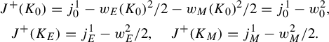 $$ \begin{gather*} J^+(K_0) = j_0^1 - w_E(K_0)^2/2 - w_M(K_0)^2/2 = j_0^1 - w_0^2, \cr J^+(K_E) = j_E^1 - w_E^2/2,\quad J^+(K_M) = j_M^1 - w_M^2/2. \end{gather*} $$
Using this and Corollary 6.15, we compute
 $$ \begin{align*} J^+(K) &= J^+(K_0)+J^+(K_E)+J^+(K_M)-2w_0\rho, \cr \mathcal{J}_0(K) &= J^+(K) + w_E(K)^2/2 + w_M(K)^2/2 \cr &= J^+(K_0) +J^+(K_E)+J^+(K_M)-2w_0\rho + (w_0+w_E)^2/2 + (w_0+w_M)^2/2 \cr &= j_0^1 + j_E^1 + j_M^1 + w_0(w_E+w_M-2\rho). \end{align*} $$
Let us denote by $L_E^{-1}(K)^1$
one component of the preimage of K under the partial regularization map at E, and similarly for
$L_E^{-1}(K)^1$
one component of the preimage of K under the partial regularization map at E, and similarly for $K_0,K_E,K_M$
. Since all winding numbers around E are even, we can choose the preimages such that
$K_0,K_E,K_M$
. Since all winding numbers around E are even, we can choose the preimages such that
 $$ \begin{align*}L_E^{-1}(K)^1 = L_E^{-1}(K_0)^1 \#_i L_E^{-1}(K_E)^1 \#_i L_E^{-1}(K_M)^1. \end{align*} $$
Let us write
 $$ \begin{align*}w_0 = 2\bar w_0. \end{align*} $$
Then $L_E^{-1}(K_0)^1$
winds around both preimages
$L_E^{-1}(K_0)^1$
winds around both preimages $M_1,M_2$
with winding number
$M_1,M_2$
with winding number $\bar w_0$
, while
$\bar w_0$
, while $L_E^{-1}(K_M)^1$
only winds with winding number
$L_E^{-1}(K_M)^1$
only winds with winding number $w_M$
around one of them, say
$w_M$
around one of them, say $M_1$
, so
$M_1$
, so
 $$ \begin{align*}w_{M_1}(L_E^{-1}(K)^1) = \bar w_0+w_M,\quad w_{M_2}(L_E^{-1}(K)^1) = \bar w_0. \end{align*} $$
Since $L_E^{-1}(K_0)^1$
is isotopic to the component
$L_E^{-1}(K_0)^1$
is isotopic to the component $\tilde K_0$
of the preimage of
$\tilde K_0$
of the preimage of $K_0$
under the map
$K_0$
under the map $z\mapsto z^2$
, using Corollary 6.15, we find
$z\mapsto z^2$
, using Corollary 6.15, we find
 $$ \begin{align*} J^+(L_E^{-1}(K)^1) &= J^+(L_E^{-1}(K_0)^1) + J^+(L_E^{-1}(K_E)^1) + J^+(L_E^{-1}(K_M)^1) - 2\bar w_0\rho, \cr &= j_0^2 + j_E^2 + J^+(K_M) - 2\bar w_0\rho, \cr \mathcal{J}_E(K) &= J^+(L_E^{-1}(K)^1) + w_{M_1}(L_E^{-1}(K)^1)^2/2 + w_{M_2}(L_E^{-1}(K)^1)^2/2 \cr &= j_0^2 + j_E^2 + J^+(K_M) - 2\bar w_0\rho + (\bar w_0+w_M)^2/2 + \bar w_0^2/2 \cr &= j_0^2 + j_E^2 + j_M^1 + \bar w_0(\bar w_0+w_M-2\rho). \end{align*} $$
Switching the roles of $E,M$
gives
$E,M$
gives
 $$ \begin{align*}\mathcal{J}_M(K) = j_0^2 + j_E^1 + j_M^2 + \bar w_0(\bar w_0+w_E-2\rho). \end{align*} $$
Finally, let $B^{-1}(K)^1$
be one component of the preimage of K under the Birkhoff regularization map, and similarly for
$B^{-1}(K)^1$
be one component of the preimage of K under the Birkhoff regularization map, and similarly for $K_0,K_E,K_M$
. Again we can choose the preimages such that
$K_0,K_E,K_M$
. Again we can choose the preimages such that
 $$ \begin{align*}B^{-1}(K)^1 = (B^{-1}(K_0)^1 \#_i B^{-1}(K_E)^1) \#_i B^{-1}(K_M)^1. \end{align*} $$
Since the preimages of $K_E,K_M$
do not wind around the origin, we have
$K_E,K_M$
do not wind around the origin, we have
 $$ \begin{align*}w_0(B^{-1}(K)^1) = w_0,\quad n(K)=|w_0|. \end{align*} $$
Since B looks like $L_E$
near E, the curve
$L_E$
near E, the curve $B^{-1}(K_E)^1$
is located near E and isotopic to
$B^{-1}(K_E)^1$
is located near E and isotopic to $L_E^{-1}(K_E)^1$
, thus
$L_E^{-1}(K_E)^1$
, thus $J^+(B^{-1}(K_E)^1) = j_E^2$
and similarly
$J^+(B^{-1}(K_E)^1) = j_E^2$
and similarly $J^+(B^{-1}(K_M)^1) = j_M^2$
. However, near infinity, B is a disconnected two-to-one covering, so
$J^+(B^{-1}(K_M)^1) = j_M^2$
. However, near infinity, B is a disconnected two-to-one covering, so $J^+(B^{-1}(K_0)^1) = J^+(K_0) = j_0^1-w_0^2$
. Using this and Corollary 6.15, we find
$J^+(B^{-1}(K_0)^1) = J^+(K_0) = j_0^1-w_0^2$
. Using this and Corollary 6.15, we find
 $$ \begin{align*} J^+(B^{-1}(K)^1) &= J^+(B^{-1}(K_0)^1) + J^+(B^{-1}(K_E)^1) + J^+(B^{-1}(K_M)^1) - 2w_0\rho \cr &= j_0^1 - w_0^2 + j_E^2 + j_M^2 - 2w_0\rho \cr &= j_0^1 + j_E^2 + j_M^2 - w_0(w_0+2\rho). \end{align*} $$
Let us now choose the rotation numbers $r_E,r_M$
such that
$r_E,r_M$
such that $\rho =0$
. With this simplification, the winding and rotation numbers of K are
$\rho =0$
. With this simplification, the winding and rotation numbers of K are
 $$ \begin{align*}(n(K),w_E(K),w_M(K),r(K)) = (|w_0|,w_0+w_E,w_0+w_M,r_0). \end{align*} $$
We see that by choosing $w_0,w_E,w_M,r_0$
, we can arrange arbitrary values in
$w_0,w_E,w_M,r_0$
, we can arrange arbitrary values in $2\mathbb {N}_0\times 2\mathbb {Z}\times 2\mathbb {Z}\times \mathbb {Z}$
for this quadruple of numbers. Fixing these choices, the four
$2\mathbb {N}_0\times 2\mathbb {Z}\times 2\mathbb {Z}\times \mathbb {Z}$
for this quadruple of numbers. Fixing these choices, the four $J^+$
-type invariants (still with
$J^+$
-type invariants (still with $\rho =0$
) were computed to be
$\rho =0$
) were computed to be
 $$ \begin{align*} \mathcal{J}_0(K) &= j_0^1 + j_E^1 + j_M^1 + w_0(w_E+w_M), \cr \mathcal{J}_E(K) &= j_0^2 + j_E^2 + j_M^1 + \bar w_0(\bar w_0+w_M), \cr \mathcal{J}_M(K) &= j_0^2 + j_E^1 + j_M^2 + \bar w_0(\bar w_0+w_E), \cr \mathcal{J}_{E,M}(K) &\equiv j_0^1 + j_E^2 + j_M^2 - w_0^2\ \mod 2n(K). \end{align*} $$
Not taking the last equation modulo $2n(K)$
, we view this as a system of four inhomogeneous linear equations in six variables
$2n(K)$
, we view this as a system of four inhomogeneous linear equations in six variables $j_0^i,j_E^i,j_M^i$
(
$j_0^i,j_E^i,j_M^i$
( $i=1,2$
) which we can choose freely in
$i=1,2$
) which we can choose freely in $2\mathbb {Z}$
. Taking the second and third equations mod
$2\mathbb {Z}$
. Taking the second and third equations mod $2$
yields
$2$
yields $\mathcal {J}_E(K)\equiv \mathcal {J}_M(K)\equiv n(K)^2/4\equiv n(K)/2$
mod
$\mathcal {J}_E(K)\equiv \mathcal {J}_M(K)\equiv n(K)^2/4\equiv n(K)/2$
mod $2$
, so relation (5) holds. Adding up the four equations yields
$2$
, so relation (5) holds. Adding up the four equations yields
 $$ \begin{align*}\mathcal{J}_0(K)+\mathcal{J}_E(K)+\mathcal{J}_M(K)+\mathcal{J}_{E,M}(K)\equiv \bar w_0(2\bar w_0+w_M+w_E) \equiv n(K)^2/2\equiv n(K)\end{align*} $$
modulo $4$
, so relation (9) holds as well. Inspection of the integer
$4$
, so relation (9) holds as well. Inspection of the integer $4\times 6$
matrix defining the equations shows that by choosing the six variables
$4\times 6$
matrix defining the equations shows that by choosing the six variables $j_0^i,j_E^i,j_M^i$
(
$j_0^i,j_E^i,j_M^i$
( $i=1,2$
), we can change
$i=1,2$
), we can change $(\mathcal {J}_0(K),\mathcal {J}_E(K),\mathcal {J}_M(K),\mathcal {J}_{E,M}(K))$
by any quadruple of even integers
$(\mathcal {J}_0(K),\mathcal {J}_E(K),\mathcal {J}_M(K),\mathcal {J}_{E,M}(K))$
by any quadruple of even integers $(a_0.a_E,a_M,a_{E,M})$
satisfying
$(a_0.a_E,a_M,a_{E,M})$
satisfying $a_0+a_E+a_M+a_{E,M}\equiv 0$
mod
$a_0+a_E+a_M+a_{E,M}\equiv 0$
mod $4$
, and therefore arrange any values compatible with relations (5) and (9).
$4$
, and therefore arrange any values compatible with relations (5) and (9).
The case with $w_E$
odd,
$w_E$
odd, $w_M$
even. We now discuss the case with
$w_M$
even. We now discuss the case with $w_{E}$
odd,
$w_{E}$
odd, $w_M$
even. The results carry over to the case with
$w_M$
even. The results carry over to the case with $w_E$
odd,
$w_E$
odd, $w_M$
even by switching the roles of E and M. By Lemmas 6.10 and 6.14, in this case,
$w_M$
even by switching the roles of E and M. By Lemmas 6.10 and 6.14, in this case, $n=0$
and the invariants take values
$n=0$
and the invariants take values $(\mathcal {J}_0,\mathcal {J}_E,\mathcal {J}_M,\mathcal {J}_{E,M})\in (2\mathbb {Z}+1/2)\times 2\mathbb {Z}\times (2\mathbb {Z}+1/2)\times 2\mathbb {Z}$
.
$(\mathcal {J}_0,\mathcal {J}_E,\mathcal {J}_M,\mathcal {J}_{E,M})\in (2\mathbb {Z}+1/2)\times 2\mathbb {Z}\times (2\mathbb {Z}+1/2)\times 2\mathbb {Z}$
.
We begin with the following refinement of [Reference Cieliebak, Frauenfelder and van Koert6, Proposition 6].
Proposition 6.19. For a generic immersed loop $K\subset \mathbb {C}\setminus \{E,M\}$
with
$K\subset \mathbb {C}\setminus \{E,M\}$
with $w_{E}(K)$
odd, we have
$w_{E}(K)$
odd, we have
 $$ \begin{align*}\mathcal{J}_{E} (K) =2 \mathcal{J}_{0}(K) -1.\end{align*} $$
If in addition $w_M(K)$
is even, then
$w_M(K)$
is even, then $\mathcal {J}_E(K)$
and
$\mathcal {J}_E(K)$
and $\mathcal {J}_{E,M}(K)$
are both divisible by four.
$\mathcal {J}_{E,M}(K)$
are both divisible by four.
Proof. Temporarily forgetting the singularity M and applying [Reference Cieliebak, Frauenfelder and van Koert6, Proposition 6] to the curve K with $w_E(K)$
odd, we get
$w_E(K)$
odd, we get
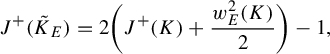 $$ \begin{align*}J^{+} (\tilde{K}_{E}) = 2 \bigg(J^{+} (K) + \dfrac{w_{E}^{2}(K)}{2}\bigg) -1,\end{align*} $$
where $\tilde K_E$
is one component of the preimage of
$\tilde K_E$
is one component of the preimage of $K_E$
under the Levi-Civita map at E. Thus,
$K_E$
under the Levi-Civita map at E. Thus,
 $$ \begin{align*}J^{+} (\tilde{K}_{E}) +w_{M}^{2} ({K}) = 2 \bigg(J^{+} (K) + \dfrac{w_{E}^{2}(K)}{2}+\dfrac{w_{M}^{2}(K)}{2}\bigg) -1.\end{align*} $$
The left-hand side is $\mathcal {J}_{E} (K)$
by Lemma 6.5, and the right-hand side is
$\mathcal {J}_{E} (K)$
by Lemma 6.5, and the right-hand side is $2 \mathcal {J}_{0}(K) -1$
by the definition of
$2 \mathcal {J}_{0}(K) -1$
by the definition of $\mathcal {J}_{0} (K)$
. This proves the first assertion.
$\mathcal {J}_{0} (K)$
. This proves the first assertion.
Suppose now that in addition, $w_M(K)$
is even. Then divisibility of
$w_M(K)$
is even. Then divisibility of $\mathcal {J}_E({K})$
by four follows from
$\mathcal {J}_E({K})$
by four follows from $\mathcal {J}_E(K)=2\mathcal {J}_0(K)-1$
and
$\mathcal {J}_E(K)=2\mathcal {J}_0(K)-1$
and $\mathcal {J}_0({K})\in 2\mathbb {Z}+1/2$
. For the last assertion, first note that a
$\mathcal {J}_0({K})\in 2\mathbb {Z}+1/2$
. For the last assertion, first note that a $(II^+)$
move on K corresponds to two
$(II^+)$
move on K corresponds to two $(II^+)$
moves on
$(II^+)$
moves on $B^{-1}(K)$
and therefore increases
$B^{-1}(K)$
and therefore increases $\mathcal {J}_{E,M}(K)$
by four. Hence, the equivalence class of
$\mathcal {J}_{E,M}(K)$
by four. Hence, the equivalence class of $\mathcal {J}_{E,M}(K)$
mod
$\mathcal {J}_{E,M}(K)$
mod $4$
does not change under arbitrary regular homotopies of K in
$4$
does not change under arbitrary regular homotopies of K in $\mathbb {C}\setminus \{E,M\}$
. It also does not change under the moves
$\mathbb {C}\setminus \{E,M\}$
. It also does not change under the moves $(I_E)$
and
$(I_E)$
and $(I_M)$
through collisions at E respectively M which change the winding numbers around E respectively M by
$(I_M)$
through collisions at E respectively M which change the winding numbers around E respectively M by $\pm 2$
. Now the free homotopy classes of loops in
$\pm 2$
. Now the free homotopy classes of loops in $\mathbb {C}\setminus \{E,M\}$
modulo the moves
$\mathbb {C}\setminus \{E,M\}$
modulo the moves $(I_E)$
and
$(I_E)$
and $(I_M)$
are in bijection to
$(I_M)$
are in bijection to $\mathbb {Z}_2\times \mathbb {Z}_2$
, classified by their winding numbers
$\mathbb {Z}_2\times \mathbb {Z}_2$
, classified by their winding numbers $w_E$
and
$w_E$
and $w_M$
mod
$w_M$
mod $2$
. Since
$2$
. Since $w_E(K)$
is odd and
$w_E(K)$
is odd and $w_M(K)$
is even, and a homotopy between immersed loops in the plane with the same rotation number can be
$w_M(K)$
is even, and a homotopy between immersed loops in the plane with the same rotation number can be $C^0$
-approximated by a regular homotopy, we can connect K by a regular homotopy in
$C^0$
-approximated by a regular homotopy, we can connect K by a regular homotopy in $\mathbb {C}\setminus \{E,M\}$
together with moves
$\mathbb {C}\setminus \{E,M\}$
together with moves $(I_E)$
and
$(I_E)$
and $(I_M)$
to a generic immersion
$(I_M)$
to a generic immersion $K_E$
located near E with
$K_E$
located near E with $w_E(K_E)=1$
and
$w_E(K_E)=1$
and $w_M(K_E)=0$
. By the preceding discussion, we have
$w_M(K_E)=0$
. By the preceding discussion, we have $\mathcal {J}_{E,M}(K_E)\equiv \mathcal {J}_{E,M}(K)$
mod
$\mathcal {J}_{E,M}(K_E)\equiv \mathcal {J}_{E,M}(K)$
mod $4$
, and
$4$
, and $\mathcal {J}_{E,M}(K_E) = \mathcal {J}_E(K_E)$
is divisible by four by the first assertion.
$\mathcal {J}_{E,M}(K_E) = \mathcal {J}_E(K_E)$
is divisible by four by the first assertion.
So $\mathcal {J}_E$
is determined by
$\mathcal {J}_E$
is determined by $\mathcal {J}_0$
and it remains to study the invariants
$\mathcal {J}_0$
and it remains to study the invariants $(\mathcal {J}_{0}, \mathcal {J}_{M}, \mathcal {J}_{E,M})\in (2\mathbb {Z}+1/2)\times (2\mathbb {Z}+1/2)\times 4\mathbb {Z}$
. We begin with the following (much simpler) analog of Lemma 6.16 for odd winding number.
$(\mathcal {J}_{0}, \mathcal {J}_{M}, \mathcal {J}_{E,M})\in (2\mathbb {Z}+1/2)\times (2\mathbb {Z}+1/2)\times 4\mathbb {Z}$
. We begin with the following (much simpler) analog of Lemma 6.16 for odd winding number.
Lemma 6.20. For any given $(j_E,w_E,r_E)\in (2\mathbb {Z}+1/2)\times (2\mathbb {Z}+1)\times \mathbb {Z}$
, there exists a generic immersed loop
$(j_E,w_E,r_E)\in (2\mathbb {Z}+1/2)\times (2\mathbb {Z}+1)\times \mathbb {Z}$
, there exists a generic immersed loop $K_E\subset \mathbb {C}\setminus \{E,M\}$
located in a small disk around E with
$K_E\subset \mathbb {C}\setminus \{E,M\}$
located in a small disk around E with
 $$ \begin{align*}(\mathcal{J}_0(K_E),w_E(K_E),r(K_E)) = (j_E,w_E,r_E). \end{align*} $$
Proof. Begin with a loop with the desired winding number $w_E$
, and take the connected sum with another loop with
$w_E$
, and take the connected sum with another loop with $w_E=0$
and prescribed
$w_E=0$
and prescribed $\mathcal {J}_0$
to arrange the desired
$\mathcal {J}_0$
to arrange the desired $\mathcal {J}_0$
. Finally, take a further connected sum with a loop with prescribed rotation number and
$\mathcal {J}_0$
. Finally, take a further connected sum with a loop with prescribed rotation number and $J^+=w_E=0$
to arrange the desired rotation number.
$J^+=w_E=0$
to arrange the desired rotation number.
We will also need the following easy lemma on rotation numbers.
Lemma 6.21. Let $K\subset \mathbb {C}^*$
be an immersed loop with winding number
$K\subset \mathbb {C}^*$
be an immersed loop with winding number $w_0(K)$
around the origin. If
$w_0(K)$
around the origin. If $w_0(K)$
is odd, the rotation numbers of K and its lift under the Levi-Civita map
$w_0(K)$
is odd, the rotation numbers of K and its lift under the Levi-Civita map $L(z)=z^2$
are related by
$L(z)=z^2$
are related by
 $$ \begin{align*}r(L^{-1}(K)) = 2r(K) - w_0(K). \end{align*} $$
If $w_0(K)$
is even, the rotation numbers of K and one component
$w_0(K)$
is even, the rotation numbers of K and one component $L^{-1}(K)^1$
of its lift under the Levi-Civita map are related by
$L^{-1}(K)^1$
of its lift under the Levi-Civita map are related by
 $$ \begin{align*}r(L^{-1}(K)^1) = r(K) - w_0(K)/2. \end{align*} $$
Proof. After a regular homotopy, we may assume that K consists of a $w_0(K)$
-fold covered circle around
$w_0(K)$
-fold covered circle around $0$
with
$0$
with $r':=r(K)-w_0(K)$
contractible circles in
$r':=r(K)-w_0(K)$
contractible circles in $\mathbb {C}^*$
attached. If
$\mathbb {C}^*$
attached. If $w_0(K)$
is odd, then
$w_0(K)$
is odd, then $L^{-1}(K)$
consists of a
$L^{-1}(K)$
consists of a $w_0(K)$
-fold covered circle around
$w_0(K)$
-fold covered circle around $0$
with
$0$
with $2r'$
contractible circles in
$2r'$
contractible circles in $\mathbb {C}^*$
attached, so its rotation number is
$\mathbb {C}^*$
attached, so its rotation number is $r(L^{-1}(K)) = w_0(K) + 2r' = 2r(K) - w_0(K)$
. If
$r(L^{-1}(K)) = w_0(K) + 2r' = 2r(K) - w_0(K)$
. If $w_0(K)$
is even, then
$w_0(K)$
is even, then $L^{-1}(K)^1$
consists of a
$L^{-1}(K)^1$
consists of a $w_0(K)/2$
-fold covered circle around
$w_0(K)/2$
-fold covered circle around $0$
with
$0$
with $r'$
contractible circles in
$r'$
contractible circles in $\mathbb {C}^*$
attached, so its rotation number is
$\mathbb {C}^*$
attached, so its rotation number is $r(L^{-1}(K)^1) = w_0(K)/2 + r' = r(K) - w_0(K)/2$
.
$r(L^{-1}(K)^1) = w_0(K)/2 + r' = r(K) - w_0(K)/2$
.
The following proposition shows that for $w_E$
odd and
$w_E$
odd and $w_M$
even, the invariants
$w_M$
even, the invariants $\mathcal {J}_0,\mathcal {J}_M,\mathcal {J}_{E,M}$
satisfy no further relations.
$\mathcal {J}_0,\mathcal {J}_M,\mathcal {J}_{E,M}$
satisfy no further relations.
Proposition 6.22. There exist generic immersed loops in $\mathbb {C}\setminus \{E,M\}$
with arbitrarily prescribed values of the invariants
$\mathbb {C}\setminus \{E,M\}$
with arbitrarily prescribed values of the invariants
 $$ \begin{align*}(\mathcal{J}_0,\mathcal{J}_M,\mathcal{J}_{E,M},w_E,w_M,r) \in (2\mathbb{Z}+1/2)\times (2\mathbb{Z}+1/2)\times 4\mathbb{Z}\times (2\mathbb{Z}+1)\times 2\mathbb{Z}\times \mathbb{Z}. \end{align*} $$
Proof. As in the proof of Proposition 6.18, we construct K as the iterated interior connected sum
 $$ \begin{align*}K := (K_0\#_iK_E)\#_iK_M\end{align*} $$
of a loop $K_E$
near E,
$K_E$
near E, $K_M$
near M, and
$K_M$
near M, and $K_0$
outside a large disk containing E and M. By Lemma 6.20, we can prescribe the invariants
$K_0$
outside a large disk containing E and M. By Lemma 6.20, we can prescribe the invariants
 $$ \begin{align*}(\mathcal{J}_{0} (K_{E}), w_{E}(K_{E}), r(K_{E}))=(j_{E}, w_{E}, r_{E}) \in (2\mathbb{Z}+1/2) \times (2 \mathbb{Z} +1) \times \mathbb{Z}\end{align*} $$
and by Lemma 6.16, we can prescribe the invariants
 $$ \begin{align*}(\mathcal{J}_{0} (K_{M}),\mathcal{J}_{M} (K_{M}), w_{M}(K_{E}), r(K_{M}))=(j^{1}_{M}, j^{2}_{M}, w_{M}, r_{M}) \in 2\mathbb{Z} \times 2\mathbb{Z} \times 2\mathbb{Z} \times \mathbb{Z},\end{align*} $$
 $$ \begin{align*}(\mathcal{J}_{0} (K_{0}),J^{+} (\tilde{K}_{0}), w_{0}(K_{0}), r(K_{0}))=(j^{1}_{0}, j^{2}_{0}, w_{0}, r_{0}) \in 2\mathbb{Z} \times 2\mathbb{Z} \times 2\mathbb{Z} \times \mathbb{Z},\end{align*} $$
where $\tilde K_0$
denotes one component of the preimage of
$\tilde K_0$
denotes one component of the preimage of $K_0$
under the Levi-Civita map
$K_0$
under the Levi-Civita map $L(z)=z^2$
. As in the proof of Proposition 6.18, we obtain
$L(z)=z^2$
. As in the proof of Proposition 6.18, we obtain
 $$ \begin{align*}w_E(K)=w_0+w_E,\quad w_M(K)=w_0+w_M,\quad r(K) = r_0+\rho,\quad \rho:= r_E+r_M+2 \end{align*} $$
and (since $w_0$
and
$w_0$
and $w_M$
are even)
$w_M$
are even)
 $$ \begin{gather*} J^{+} (K_{0})=j_{0}^{1}-w_{0}^{2},\quad J^{+}(K_{E})=j_{E}-w_{E}^{2}/2,\quad J^{+}(K_{M})=j_{M}^{1}-w_{M}^{2}/2, \cr \mathcal{J}_0(K) = j_0^1 + j_E + j_M^1 + w_0(w_E+w_M-2\rho),\cr \mathcal{J}_M(K) = j_0^2 + j_E + j_M^2 + w_0(w_0+w_E-2\rho). \end{gather*} $$
To compute $\mathcal {J}_{E.M}(K)$
, let
$\mathcal {J}_{E.M}(K)$
, let $B^{-1}(K_{0})^{1,2}$
and
$B^{-1}(K_{0})^{1,2}$
and $B^{-1}(K_{M})^{1,2}$
be the connected components of the preimages of
$B^{-1}(K_{M})^{1,2}$
be the connected components of the preimages of $K_0$
respectively
$K_0$
respectively $K_M$
under the Birkhoff map
$K_M$
under the Birkhoff map $B:\mathbb {C}^*\to \mathbb {C}$
. Here, we label
$B:\mathbb {C}^*\to \mathbb {C}$
. Here, we label $B^{-1}(K_{0})^{1}$
the component inside the unit disk and by
$B^{-1}(K_{0})^{1}$
the component inside the unit disk and by $B^{-1}(K_{0})^{2}$
the one outside. We choose
$B^{-1}(K_{0})^{2}$
the one outside. We choose $w_M\neq 0$
and arrange for
$w_M\neq 0$
and arrange for $K_{M}$
the additional property in Lemma 6.16 that the two components of
$K_{M}$
the additional property in Lemma 6.16 that the two components of $B^{-1}(K_{M})$
can be disjoined by a regular homotopy involving only inverse self-tangencies. We label
$B^{-1}(K_{M})$
can be disjoined by a regular homotopy involving only inverse self-tangencies. We label $B^{-1}(K_{M})^{1}$
the component that is connected to
$B^{-1}(K_{M})^{1}$
the component that is connected to $B^{-1}(K_{0})^{1}$
by the connected sum construction, and by
$B^{-1}(K_{0})^{1}$
by the connected sum construction, and by $B^{-1}(K_{M})^{2}$
the one connected to
$B^{-1}(K_{M})^{2}$
the one connected to $B^{-1}(K_{0})^{2}$
. Then, the preimage
$B^{-1}(K_{0})^{2}$
. Then, the preimage $B^{-1}(K)$
looks like in Figure 9. Disjoining the two components of
$B^{-1}(K)$
looks like in Figure 9. Disjoining the two components of $B^{-1}(K_{M})$
in
$B^{-1}(K_{M})$
in $B^{-1}(K)$
through inverse self-tangencies and pushing
$B^{-1}(K)$
through inverse self-tangencies and pushing $B^{-1}(K_0)^1$
away from
$B^{-1}(K_0)^1$
away from $0$
does not change
$0$
does not change $J^+$
, so it leads to a curve
$J^+$
, so it leads to a curve $K'$
with
$K'$
with $J^+(K')=\mathcal {J}_{E,M}(K)$
which can be written as an iterated connected/interior connected sum
$J^+(K')=\mathcal {J}_{E,M}(K)$
which can be written as an iterated connected/interior connected sum
 $$ \begin{align*}K'=K'_2\#_iK'_1\end{align*} $$
with
 $$ \begin{align*}K_2'=B^{-1}(K_{0})^{2} \#_i B^{-1}(K_{M})^{2},\quad K_1'=(B^{-1}(K_{E})\#B^{-1}(K_{0})^{1})\# B^{-1}(K_{M})^{1}.\end{align*} $$
Note that since the interior connected sums are formed by positive bases, the mirrored connected sums involved are also formed by positive bases, so their rotation numbers obey formula (6).
The case with $w_E$
odd,
$w_E$
odd, $w_M$
even.
$w_M$
even.

To compute $J^{+}(K')$
(and thus
$J^{+}(K')$
(and thus $\mathcal {J}_{E, M} (K)$
), recall that the Birkhoff map behaves like the map
$\mathcal {J}_{E, M} (K)$
), recall that the Birkhoff map behaves like the map $z\mapsto z/2$
near infinity and like the respective Levi-Civita maps near E and M. In particular,
$z\mapsto z/2$
near infinity and like the respective Levi-Civita maps near E and M. In particular, $B^{-1}(K_{0})^{2}$
is diffeomorphic to
$B^{-1}(K_{0})^{2}$
is diffeomorphic to $K_{0}$
and thus has the same invariants. Using this and Lemma 6.21, we compute the rotation numbers
$K_{0}$
and thus has the same invariants. Using this and Lemma 6.21, we compute the rotation numbers
 $$ \begin{align*}r(B^{-1}(K_0)^{2})=r_0,\quad r(B^{-1}(K_E))=2r_E-w_E,\quad r(B^{-1}(K_M)^{1,2})=r_M-w_M/2. \end{align*} $$
From Lemma 6.8, we infer
 $$ \begin{align*}r(B^{-1}(K_0)^1)=r_0-2w_0,\end{align*} $$
whence in view of formula (6),
 $$ \begin{align*} r(K_1') &= r(B^{-1} (K_{E}))+r(B^{-1}(K_{0})^{1}) + r(B^{-1}(K_{M})^{1})+2 \cr &= 2r_{E}-w_{E}+r_{0}-2w_0+r_M-w_M/2+2. \end{align*} $$
Using repeatedly equation (4), Corollary 6.15, and Proposition 6.19, we now compute the $J^+$
-invariants:
$J^+$
-invariants:
 $$ \begin{align*} J^+(B^{-1}(K_0)^2) &= J^{+}(K_{0}) = j_0^1-w_0^2, \\[2pt] J^+(B^{-1}(K_M)^{1,2}) &= j_M^2, \\[2pt] J^+(K_2') &= J^+(B^{-1}(K_0)^2) + J^+(B^{-1}(K_M)^2) \\[2pt] &\quad- 2w_0(B^{-1}(K_0)^2) (r(B^{-1}(K_M)^2)+1) \\[2pt] &= j_0^1-w_0^2+j_M^2-2w_0(r_M-w_M/2+1), \\[2pt] J^+(B^{-1}(K_E)) &= 2J^+(K_E)+w_E(K_E)^2-1 = 2j_E-w_E^2+w_E^2-1 \\[2pt] &= 2j_E-1, \\[2pt] J^+(B^{-1}(K_0)^1) &= J^+(B^{-1}(K_0)^2)+2w_0(r_0-w_0) \\[2pt] &= j_0^1-w_0^2+2w_0(r_0-w_0) = j_0^1-3w_0^2+2w_0r_0, \\[2pt] J^+(K_1') &= J^+(B^{-1}(K_E)) + J^+(B^{-1}(K_0)^1) + J^+(B^{-1}(K_M)^1) \\[2pt] &= 2j_E-1 + j_0^1-3w_0^2+2w_0r_0 + j_M^2, \\[2pt] \mathcal{J}_{E,M}(K) &= J^+(K') = J^+(K_2') + J^+(K_1') - 2w_0(K_2')(r(K_1')+1) \\[2pt] &= j_0^1-w_0^2+j_M^2-2w_0(r_M+1)+w_0w_M \\[2pt] &\quad + 2j_E-1+j_0^1-3w_0^2+2w_0r_0+j_M^2 \\[2pt] &\quad -2w_0(2r_{E}-w_{E}+r_{0}+r_M-2w_0-w_M/2+2+1) \\[2pt] &= 2j_0^1+2j_E+2j_M^2+2w_0(w_E+w_M)-4w_0\rho-1. \end{align*} $$
Let us now choose the rotation numbers $r_E,r_M$
such that
$r_E,r_M$
such that $\rho =0$
. With this simplification, the winding and rotation numbers of K are
$\rho =0$
. With this simplification, the winding and rotation numbers of K are
 $$ \begin{align*}(w_E(K),w_M(K),r(K)) = (w_0+w_E,w_0+w_M,r_0). \end{align*} $$
We see that by fixing some $w_M\neq 0$
(which was needed above to apply Lemma 6.16) and varying
$w_M\neq 0$
(which was needed above to apply Lemma 6.16) and varying $w_0,w_E,r_0$
, we can arrange arbitrary values in
$w_0,w_E,r_0$
, we can arrange arbitrary values in $\mathbb {Z}\times 2\mathbb {Z}\times \mathbb {Z}$
for this triple of numbers. Fixing these choices, the three
$\mathbb {Z}\times 2\mathbb {Z}\times \mathbb {Z}$
for this triple of numbers. Fixing these choices, the three $J^+$
-like invariants (still with
$J^+$
-like invariants (still with $\rho =0$
) were computed to be
$\rho =0$
) were computed to be
 $$ \begin{align*} \mathcal{J}_0(K) &= j_0^1 + j_E + j_M^1 + w_0(w_E+w_M) \in 2\mathbb{Z}+1/2, \\[3pt] \mathcal{J}_M(K) &= j_0^2 + j_E + j_M^2 + w_0(w_0+w_E)\in 2\mathbb{Z}+1/2, \\[3pt] \mathcal{J}_{E,M}(K) &= 2j_0^1+2j_E+2j_M^2+2w_0(w_E+w_M)-1\in 4\mathbb{Z}. \end{align*} $$
We view this as a system of three inhomogeneous linear equations in five variables $(j_E,j_M^1,j_M^2,j_0^1,j_0^2)\in (2\mathbb {Z}+1/2)\times 2\mathbb {Z}\times 2\mathbb {Z}\times 2\mathbb {Z}\times 2\mathbb {Z}$
, which we can choose freely. Inspection of the integer
$(j_E,j_M^1,j_M^2,j_0^1,j_0^2)\in (2\mathbb {Z}+1/2)\times 2\mathbb {Z}\times 2\mathbb {Z}\times 2\mathbb {Z}\times 2\mathbb {Z}$
, which we can choose freely. Inspection of the integer $3\times 5$
matrix defining the equations shows that by varying
$3\times 5$
matrix defining the equations shows that by varying $(j_E,j_M^1,j_M^2,j_0^1,j_0^2)$
, we can change
$(j_E,j_M^1,j_M^2,j_0^1,j_0^2)$
, we can change $(\mathcal {J}_0(K),\mathcal {J}_M(K),\mathcal {J}_{E,M}(K))$
by any triple in
$(\mathcal {J}_0(K),\mathcal {J}_M(K),\mathcal {J}_{E,M}(K))$
by any triple in $2\mathbb {Z}\times 2\mathbb {Z}\times 4\mathbb {Z}$
, and therefore arrange any values in
$2\mathbb {Z}\times 2\mathbb {Z}\times 4\mathbb {Z}$
, and therefore arrange any values in $(2\mathbb {Z}+1/2)\times (2\mathbb {Z}+1.2)\times 4\mathbb {Z}$
.
$(2\mathbb {Z}+1/2)\times (2\mathbb {Z}+1.2)\times 4\mathbb {Z}$
.
The case with $w_E,w_M$
odd. By Lemmas 6.10 and 6.14, in this case, n is odd and
$w_E,w_M$
odd. By Lemmas 6.10 and 6.14, in this case, n is odd and $(\mathcal {J}_0,\mathcal {J}_E,\mathcal {J}_M,\mathcal {J}_{E,M})\in (2\mathbb {Z}+1)\times (2\mathbb {Z}+1)\times (2\mathbb {Z}+1)\times 2\mathbb {Z}/2n\mathbb {Z}$
. Moreover, Proposition 6.19 immediately implies the following corollary.
$(\mathcal {J}_0,\mathcal {J}_E,\mathcal {J}_M,\mathcal {J}_{E,M})\in (2\mathbb {Z}+1)\times (2\mathbb {Z}+1)\times (2\mathbb {Z}+1)\times 2\mathbb {Z}/2n\mathbb {Z}$
. Moreover, Proposition 6.19 immediately implies the following corollary.
Corollary 6.23. If $w_{E} (K)$
and
$w_{E} (K)$
and $w_{M} (K)$
are both odd, then
$w_{M} (K)$
are both odd, then
 $$ \begin{align*}\mathcal{J}_{E}(K)=\mathcal{J}_{M}(K)=2 \mathcal{J}_{0}(K) -1.\end{align*} $$
So $\mathcal {J}_E,\mathcal {J}_M$
are determined by
$\mathcal {J}_E,\mathcal {J}_M$
are determined by $\mathcal {J}_0$
. The following proposition shows that
$\mathcal {J}_0$
. The following proposition shows that $\mathcal {J}_{0}$
and
$\mathcal {J}_{0}$
and $\mathcal {J}_{E, M}$
satisfy no further relations.
$\mathcal {J}_{E, M}$
satisfy no further relations.
Proposition 6.24. There exist generic immersed loops in $\mathbb {C}\setminus \{E,M\}$
with arbitrarily prescribed values of the invariants
$\mathbb {C}\setminus \{E,M\}$
with arbitrarily prescribed values of the invariants
 $$ \begin{align*}(\mathcal{J}_0,\mathcal{J}_{E,M},n,w_E,w_M,r) \in (2\mathbb{Z}+1)\times 2\mathbb{Z}/2n\mathbb{Z}\times (2N_0+1)\times (2\mathbb{Z}+1)\times (2\mathbb{Z}+1) \times \mathbb{Z}. \end{align*} $$
Proof. As in the proof of Proposition 6.18, we construct K as the iterated interior connected sum
 $$ \begin{align*}K := (K_0\#_iK_E)\#_iK_M\end{align*} $$
of a loop $K_E$
near E,
$K_E$
near E, $K_M$
near M, and
$K_M$
near M, and $K_0$
outside a large disk containing E and M. We choose the winding number
$K_0$
outside a large disk containing E and M. We choose the winding number $w_0(K_0)$
odd and the winding numbers
$w_0(K_0)$
odd and the winding numbers $w_E(K_E),w_M(K_M)$
even. Then by Lemma 6.20, we can prescribe the invariants
$w_E(K_E),w_M(K_M)$
even. Then by Lemma 6.20, we can prescribe the invariants
 $$ \begin{align*}(\mathcal{J}_0(K_0), w_0(K_0), r(K_0))=(j_0^1, w_0, r_0) \in (2\mathbb{Z}+1) \times (2\mathbb{Z} +1) \times \mathbb{Z}\end{align*} $$
and by Lemma 6.16, we can prescribe the invariants
 $$ \begin{align*}(\mathcal{J}_0(K_E),\mathcal{J}_E(K_E), w_E(K_E), r(K_E))=(j^1_E, j^2_E, w_E, r_E) \in 2\mathbb{Z} \times 2\mathbb{Z} \times 2\mathbb{Z} \times \mathbb{Z},\end{align*} $$
 $$ \begin{align*}(\mathcal{J}_0(K_M),\mathcal{J}_M(K_M), w_M(K_M), r(K_M))=(j^1_M, j^2_M, w_M, r_M) \in 2\mathbb{Z} \times 2\mathbb{Z} \times 2\mathbb{Z} \times \mathbb{Z}.\end{align*} $$
As in the proof of Proposition 6.18, we obtain
 $$ \begin{align*}w_E(K)=w_0+w_E,\quad w_M(K)=w_0+w_M,\quad r(K) = r_0+\rho,\quad \rho:= r_E+r_M+2 \end{align*} $$
and (since $w_E$
,
$w_E$
, $w_M$
are even and the parity of
$w_M$
are even and the parity of $w_0$
played no role in the computation of these two invariants)
$w_0$
played no role in the computation of these two invariants)
 $$ \begin{align*} \mathcal{J}_0(K) &= j_0^1 + j_E^1 + j_M^1 + w_0(w_E+w_M), \\[3pt] \mathcal{J}_{E,M}(K) &\equiv j_0^1 + j_E^2 + j_M^2 - w_0^2\ \mod 2n(K), \end{align*} $$
where $n(K)=|w_0|$
and we have again chosen
$n(K)=|w_0|$
and we have again chosen $r_E,r_M$
such that
$r_E,r_M$
such that $\rho =0$
. Hence, by varying
$\rho =0$
. Hence, by varying $(w_0,w_E,w_M,r_0)$
, we can arrange arbitrary values for
$(w_0,w_E,w_M,r_0)$
, we can arrange arbitrary values for
 $$ \begin{align*}(n(K),w_E(K),w_M(K),r(K)) \in (2N_0+1)\times (2\mathbb{Z}+1)\times (2\mathbb{Z}+1) \times \mathbb{Z},\end{align*} $$
and given these, by varying $(j_0^1,j_E^1,j_E^2,j_M^1,j_M^2)$
, we can arrange arbitrary values for
$(j_0^1,j_E^1,j_E^2,j_M^1,j_M^2)$
, we can arrange arbitrary values for $(\mathcal {J}_0,\mathcal {J}_{E,M})\in (2\mathbb {Z}+1)\times 2\mathbb {Z}/2n\mathbb {Z}$
.
$(\mathcal {J}_0,\mathcal {J}_{E,M})\in (2\mathbb {Z}+1)\times 2\mathbb {Z}/2n\mathbb {Z}$
.
7 Further discussions
7.1 Knot types and Legendrian knots
As in the one-center case discussed in [Reference Cieliebak, Frauenfelder and van Koert6], each periodic orbit of a two-center Stark–Zeeman system describes an oriented knot in the Moser-regularized energy hypersurface $\Sigma _c^M\cong \mathbb {R} P^3\#\mathbb {R} P^3$
, which has been shown in the planar circular restricted three-body problem for energy values slightly above the first critical value to be of contact type in [Reference Albers, Frauenfelder, van Koert and Paternain1], and each generic immersion
$\Sigma _c^M\cong \mathbb {R} P^3\#\mathbb {R} P^3$
, which has been shown in the planar circular restricted three-body problem for energy values slightly above the first critical value to be of contact type in [Reference Albers, Frauenfelder, van Koert and Paternain1], and each generic immersion $K\subset \mathbb {C}\setminus \{E,M\}$
lifts (by adding its tangent direction) to an oriented knot in
$K\subset \mathbb {C}\setminus \{E,M\}$
lifts (by adding its tangent direction) to an oriented knot in $\gamma \subset \mathbb {R} P^3\#\mathbb {R} P^3$
whose knot type is invariant under Stark–Zeeman homotopies. Note that according to Lemma 6.14, the free homotopy class of
$\gamma \subset \mathbb {R} P^3\#\mathbb {R} P^3$
whose knot type is invariant under Stark–Zeeman homotopies. Note that according to Lemma 6.14, the free homotopy class of $\gamma $
is captured by the invariants
$\gamma $
is captured by the invariants $\mathcal {J}_E(K)$
,
$\mathcal {J}_E(K)$
, $\mathcal {J}_M(K)$
, and
$\mathcal {J}_M(K)$
, and $n(K)$
. The proof of [Reference Cieliebak, Frauenfelder and van Koert6, Corollary 3] shows that every oriented knot type in
$n(K)$
. The proof of [Reference Cieliebak, Frauenfelder and van Koert6, Corollary 3] shows that every oriented knot type in $\mathbb {R} P^3\#\mathbb {R} P^3$
is realized by a Moser regularized periodic orbit in some two-center Stark–Zeeman system. A periodic orbit in
$\mathbb {R} P^3\#\mathbb {R} P^3$
is realized by a Moser regularized periodic orbit in some two-center Stark–Zeeman system. A periodic orbit in $\Sigma _c^M\cong \mathbb {R} P^3\#\mathbb {R} P^3$
can be further lifted to an oriented knot in the Birkhoff regularized energy hypersurface
$\Sigma _c^M\cong \mathbb {R} P^3\#\mathbb {R} P^3$
can be further lifted to an oriented knot in the Birkhoff regularized energy hypersurface $\Sigma _c^B\cong S^1\times S^2$
whose knot type is also invariant under Stark–Zeeman homotopies of its footpoint projection.
$\Sigma _c^B\cong S^1\times S^2$
whose knot type is also invariant under Stark–Zeeman homotopies of its footpoint projection.
As mentioned in [Reference Cieliebak, Frauenfelder and van Koert6], it would be interesting to search for more refined invariants under one- or two-center Stark–Zeeman homotopies using invariants of their Legendrian lifts (by adding the unit conormal vectors).
7.2 N-center Stark–Zeeman systems
The notions of planar one- and two-center Stark–Zeeman systems generalize in the obvious way to that of a planar N-center Stark–Zeeman system. On a given energy level, a partial Levi-Civita regularization at some subset of the N centers can be defined by going to a Riemann surface branched at these centers, see Klein and Knauf [Reference Klein and Knauf11]. This should give rise to $2^N$
different
$2^N$
different $J^+$
-like invariants for periodic orbits of a planar N-center Stark–Zeeman system, which would be interesting to be further explored.
$J^+$
-like invariants for periodic orbits of a planar N-center Stark–Zeeman system, which would be interesting to be further explored.
Acknowledgements
K.C. was partially supported by DFG grant CI 45/8-1. U.F. was partially supported by DFG grant FR 2637/2-2. L.Z. was partially supported by DFG grant ZH 605/1-1.


 Open access