



1. Introduction
The motivation of the model uncertainty/ambiguity topic stems from the fact that the presence of a family of probability measures, which are singular from each other, in studying super hedging price and risk measuring problems is inevitable. In fact, since a family of martingale probability measures leads to incompleteness, it is impossible to perfectly replicate hedges with certainty.
Faced with such circumstances, several recent efforts have been put into developing the theory of arbitrage-free pricing under ambiguity, where there is a lack of consensus among the probability assignments. The optimal super-replication price of a European contingent claim in the context of uncertainty with (non-dominated) martingale probability measures was acquired in [Reference Denis and Martini7]. By focusing on ambiguity about both drift and volatility in a continuous-time framework, [Reference Epstein and Ji8, Reference Epstein and Ji9] formulated a model of utility that captures the decision-maker’s concern under ambiguity. The reader can refer to [Reference Nutz. and Soner21, Reference Nutz and Van Handel22, Reference Soner, Touzi and Zhang25] and the references therein for more detailed discussions.
In order to study the problem of ambiguity, [Reference Peng23, Reference Peng24] developed the G-expectation theory and G-Itô stochastic calculus, which systematically established a framework of time-consistent sublinear expectation.
Since the stochastic differential equations driven by G-Brownian motion (G-SDEs for short) have a pivotal role in modeling financial processes, they have attracted a great deal of attention from researchers. For instance, [Reference Akhtari, Biagini, Mazzon and Oberpriller2] is devoted to studying the G-conditional expectation of a discounted payoff related to a sufficiently smooth G-SDE, which is obtained by a generalization of a Feynmac–Kac formula under volatility uncertainty. Also, the property of continuous dependence on the parameters of stochastic integrals and solutions of G-SDEs was studied in [Reference Lin16]. The pathwise properties and homeomorphic ones with respect to the initial values for such equations were established in [Reference Gao10]. The authors in [Reference Deng, Fei, Fei and Mao6] proved that the stochastic stability of stochastic delay differential equations driven by G-Brownian motion is equivalent to that of the Euler–Maruyama scheme. In [Reference Akhtari1], a split-step backward Euler–Maryuama scheme was employed to approximate the solution and the pathwise convergence of the scheme was proved.
Most of the results in the literature are concerned with G-SDEs under standard assumptions. However, recently, some research has been dedicated to the G-SDEs which possess more complex coefficients. Both the existence and uniqueness of the solution of G-SDEs under integral-Lipschitz conditions were investigated in [Reference Bai and Lin4]. In [Reference Akhtari and Li3], the existence and uniqueness of the solution of the Cox–Ingersoll–Ross process driven by G-Brownian motion was provided, and some of its properties, including the Markov property and its distribution, were indicated.
We might need to equip ourselves with more advanced instruments of G-stochastic calculus in order to study G-SDEs with less smoothness. For instance, the integrand space of the first definition of the G-Itô integral is restricted to stochastic processes that are continuous in $\omega$
, while it might be required to define the G-Itô integral for processes that are beyond the quasi-continuous space. In particular, this is relevant to the case of the G-Itô integral on
$\omega$
, while it might be required to define the G-Itô integral for processes that are beyond the quasi-continuous space. In particular, this is relevant to the case of the G-Itô integral on $[0, \tau]$
where
$[0, \tau]$
where $\tau$
is a stopping time; stopping time is a delicate issue in the G-framework and may no longer be quasi-continuous unless some strong conditions are imposed—see [Reference Liu17] to more details.
$\tau$
is a stopping time; stopping time is a delicate issue in the G-framework and may no longer be quasi-continuous unless some strong conditions are imposed—see [Reference Liu17] to more details.
To overcome this difficulty, [Reference Li and Peng15] extended the definition of the G-Itô integral to the larger spaces $M^2_{\star}([0, T])$
and
$M^2_{\star}([0, T])$
and $M^2_{\unicode{x03C9}}([0, T])$
that contain processes that are not necessarily quasi-continuous, and also we have
$M^2_{\unicode{x03C9}}([0, T])$
that contain processes that are not necessarily quasi-continuous, and also we have $M^2_G([0,T]) \subset M^2_{\star}([0,T]) \subset M^2_{\unicode{x03C9}}([0, T])$
.
$M^2_G([0,T]) \subset M^2_{\star}([0,T]) \subset M^2_{\unicode{x03C9}}([0, T])$
.
The existence and uniqueness of the solution of G-SDEs with local Lipschitz coefficients under a Lyapunov-type condition are dealt with in [Reference Li, Lin and Lin13], which also studies the stability of the equation under any arbitrarily small perturbation of the initial value of the solution. They benefited from [Reference Li and Peng15] to find the solution of the equation in the $M_{\unicode{x03C9}}([0, T])$
space by a localization technique. Motivated by the aforementioned paper studying G-SDEs under locally Lipschitz continuous coefficients, we develop a numerical scheme for the solution of the equation and then prove its convergence and asymptotic stability properties.
$M_{\unicode{x03C9}}([0, T])$
space by a localization technique. Motivated by the aforementioned paper studying G-SDEs under locally Lipschitz continuous coefficients, we develop a numerical scheme for the solution of the equation and then prove its convergence and asymptotic stability properties.
To this end, numerical solutions of stochastic differential equations driven by classical Brownian motion, in which the coefficients do not obey the global Lipschitz condition, can be an inspiration for the G-SDE case. For instance, a numerical solution for SDEs with non-linear and non-Lipschitz coefficients is presented in [Reference Mao and Szpruch20], and its strong convergence and almost sure stability are proved. In [Reference Higham, Mao and Stuart12], an SDE satisfying only a local Lipschitz property is considered. Then the strong convergence of the Euler–Maruyama scheme and also the boundedness of the pth moments of the exact and numerical solutions are investigated for some $p > 2$
. Moreover, an Euler–Maruyama-type method in [Reference Mao and Sabanis19] is applied to the numerical solutions for stochastic differential delay equations with variable delay under the local Lipschitz condition.
$p > 2$
. Moreover, an Euler–Maruyama-type method in [Reference Mao and Sabanis19] is applied to the numerical solutions for stochastic differential delay equations with variable delay under the local Lipschitz condition.
Besides Euler-type schemes, the so-called $\theta$
-schemes include both explicit and implicit methods governed by a parameter
$\theta$
-schemes include both explicit and implicit methods governed by a parameter $\theta \in [0, 1]$
. In [Reference Higham11], a stochastic variant of the theta method is employed to approximate a linear test SDE with multiplicative noise, and the mean-square and asymptotic stability properties are subsequently analyzed. Moreover, the authors in [Reference Chen, Cao and Chen5] apply stochastic theta methods to find random periodic solutions of stochastic differential equations under non-globally Lipschitz conditions. The split-step theta method, addressing a class of SDEs with piecewise continuous arguments and polynomial growth conditions, is investigated in [Reference Lu, Song and Liu18]. Additional relevant studies can be found in [Reference Wang, Wu and Dong26, Reference Wu and Gan27]. Inspired by these
$\theta \in [0, 1]$
. In [Reference Higham11], a stochastic variant of the theta method is employed to approximate a linear test SDE with multiplicative noise, and the mean-square and asymptotic stability properties are subsequently analyzed. Moreover, the authors in [Reference Chen, Cao and Chen5] apply stochastic theta methods to find random periodic solutions of stochastic differential equations under non-globally Lipschitz conditions. The split-step theta method, addressing a class of SDEs with piecewise continuous arguments and polynomial growth conditions, is investigated in [Reference Lu, Song and Liu18]. Additional relevant studies can be found in [Reference Wang, Wu and Dong26, Reference Wu and Gan27]. Inspired by these $\theta$
-schemes for SDEs, we adopt a similar approach to develop an approximation method for the G-SDE under study.
$\theta$
-schemes for SDEs, we adopt a similar approach to develop an approximation method for the G-SDE under study.
The rest of the paper is arranged as follows. Section 2 is devoted to the necessary preliminaries of G-expectation theory. In Section 3, we study the theoretical property of G-SDEs under the locally Lipschitz condition. In Section 4, we introduce an implicit continuous Euler–Maruyama scheme to approximate the solution of the associated equation and then the convergence and stability of the scheme are examined. Section 5 introduces two test problems to illustrate the theoretical findings.
2. Preliminaries
In this section we review some necessary preliminaries on G-Brownian motion calculus to be used throughout the paper. Let $\Omega \, :\!= \, C^d_0(\mathbb{R}^+)$
be the space of all
$\Omega \, :\!= \, C^d_0(\mathbb{R}^+)$
be the space of all $\mathbb{R}^d$
-valued continuous paths
$\mathbb{R}^d$
-valued continuous paths $(\omega_t)_{t \in \mathbb{R}^{+}}$
with
$(\omega_t)_{t \in \mathbb{R}^{+}}$
with $\omega_0 = 0$
equipped with the distance
$\omega_0 = 0$
equipped with the distance
 \begin{equation*}\rho(\omega^1\!, \omega^2) \, :\!= \, \sum_{i=1}^{\infty}2^{-i}\Big[\Big(\max_{t \in [0, i]} \rvert\omega^1_t - \omega^2_t\rvert \Big) \wedge 1\Big], \quad \omega^1\!, \omega^2 \in \Omega.\end{equation*}
Let $t \in [0, \infty)$
. Define
$t \in [0, \infty)$
. Define $\Omega_t\, :\!= \,\{\omega_{\cdot \wedge t}\colon \omega\in\Omega\}$
and consider the canonical process
$\Omega_t\, :\!= \,\{\omega_{\cdot \wedge t}\colon \omega\in\Omega\}$
and consider the canonical process $B_t(\omega) = \omega_t$
for
$B_t(\omega) = \omega_t$
for $\omega \in \Omega$
. Set
$\omega \in \Omega$
. Set
 $$\operatorname{Lip}\!(\Omega_t)\, :\!= \,\{\varphi(B_{t_1 \wedge t},\ldots,B_{t_n \wedge t})\colon \text{for all}\ n\in\mathbb{N},\ t_i \geq 0, \varphi \in C_\mathrm{l. Lip}(\mathbb{R}^n)\},$$
where $a \wedge b = \min \{a,b\}$
and we denote by
$a \wedge b = \min \{a,b\}$
and we denote by $C_\mathrm{l. Lip}(\mathbb{R}^n)$
the linear space of functions
$C_\mathrm{l. Lip}(\mathbb{R}^n)$
the linear space of functions $\varphi$
satisfying the local Lipschitz condition
$\varphi$
satisfying the local Lipschitz condition $|\varphi(x) - \varphi(y)| \leq C(1 + |x|^m + |y|^m)|x - y|$
for
$|\varphi(x) - \varphi(y)| \leq C(1 + |x|^m + |y|^m)|x - y|$
for $x, y \in \mathbb{R}^n$
, where the constant
$x, y \in \mathbb{R}^n$
, where the constant $C>0$
and the integer
$C>0$
and the integer $m \in \mathbb{N}$
depend on
$m \in \mathbb{N}$
depend on $\varphi$
. Set
$\varphi$
. Set $\mathrm{Lip}(\Omega) \, :\!= \, \bigcup_{n}{\mathrm{Lip}(\Omega_n)}$
, which reveals a linear space of real-valued functions defined on
$\mathrm{Lip}(\Omega) \, :\!= \, \bigcup_{n}{\mathrm{Lip}(\Omega_n)}$
, which reveals a linear space of real-valued functions defined on $\Omega$
and constructs a vector lattice. Let
$\Omega$
and constructs a vector lattice. Let $\hat{\mathbb E}$
be a functional defined on
$\hat{\mathbb E}$
be a functional defined on $\mathrm{Lip}(\Omega)$
satisfying the monotonicity, preservation of constants, sub-additivity, and positive homogenity properties. The functional
$\mathrm{Lip}(\Omega)$
satisfying the monotonicity, preservation of constants, sub-additivity, and positive homogenity properties. The functional $\hat{\mathbb E}$
is called a sublinear expectation and the triple
$\hat{\mathbb E}$
is called a sublinear expectation and the triple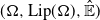 $(\Omega, \mathrm{Lip}(\Omega), \hat{\mathbb E})$
a sublinear expectation space. [Reference Peng24] constructs a sublinear expectation
$(\Omega, \mathrm{Lip}(\Omega), \hat{\mathbb E})$
a sublinear expectation space. [Reference Peng24] constructs a sublinear expectation $\hat{\mathbb E}$
on
$\hat{\mathbb E}$
on $(\Omega, \mathrm{Lip}(\Omega))$
called the G-expectation. Note that
$(\Omega, \mathrm{Lip}(\Omega))$
called the G-expectation. Note that $\mathrm{Lip}(\Omega)$
can be extended to
$\mathrm{Lip}(\Omega)$
can be extended to $L^p_G(\Omega)$
for
$L^p_G(\Omega)$
for $p \geq 1$
, which denotes the completion of
$p \geq 1$
, which denotes the completion of $\mathrm{Lip}(\Omega)$
under
$\mathrm{Lip}(\Omega)$
under $\|X\|_p \, :\!= \, (\hat{\mathbb E}[|X|^p])^{{1}/{p}}$
for
$\|X\|_p \, :\!= \, (\hat{\mathbb E}[|X|^p])^{{1}/{p}}$
for $X \in \mathrm{Lip}(\Omega)$
.
$X \in \mathrm{Lip}(\Omega)$
.
We denote by $\mathcal{P}$
a weakly compact but possibly non-dominated family of probability measures that represents
$\mathcal{P}$
a weakly compact but possibly non-dominated family of probability measures that represents $\hat{\mathbb E}$
as
$\hat{\mathbb E}$
as $\hat{\mathbb E}[X] = \sup\nolimits_{P \in \mathcal{P}} E_{P}[X]$
for
$\hat{\mathbb E}[X] = \sup\nolimits_{P \in \mathcal{P}} E_{P}[X]$
for $X \in \mathrm{Lip}(\Omega)$
, where
$X \in \mathrm{Lip}(\Omega)$
, where $\{E_P \colon P \in \mathcal{P}\}$
represents a subset of linear expectations. We denote by
$\{E_P \colon P \in \mathcal{P}\}$
represents a subset of linear expectations. We denote by $\mathcal{B}(\Omega)$
the Borel
$\mathcal{B}(\Omega)$
the Borel $\sigma$
-algebra of
$\sigma$
-algebra of $\Omega$
. The capacity associated with
$\Omega$
. The capacity associated with $\mathcal{P}$
is denoted by
$\mathcal{P}$
is denoted by ${c}(A) \, :\!= \, \sup\nolimits_{P \in \mathcal{P}} P(A)$
,
${c}(A) \, :\!= \, \sup\nolimits_{P \in \mathcal{P}} P(A)$
, $A \in \mathcal{B}(\Omega)$
. A set A is polar if
$A \in \mathcal{B}(\Omega)$
. A set A is polar if $c(A) = 0$
and a property holds ‘quasi-surely’ (q.s.) if it holds outside a polar set.
$c(A) = 0$
and a property holds ‘quasi-surely’ (q.s.) if it holds outside a polar set.
Let $(\Omega,{\mathcal H}, \hat{\mathbb E})$
be a sublinear expectation space, i.e.
$(\Omega,{\mathcal H}, \hat{\mathbb E})$
be a sublinear expectation space, i.e. ${\mathcal H}$
is a linear space of real-valued functions defined on
${\mathcal H}$
is a linear space of real-valued functions defined on $\Omega$
and constructs a vector lattice, and
$\Omega$
and constructs a vector lattice, and $\hat{\mathbb E}$
is a sublinear expectation on
$\hat{\mathbb E}$
is a sublinear expectation on ${\mathcal H}$
. The space
${\mathcal H}$
. The space ${\mathcal H}$
is considered as the space of ‘random variables’. Moreover, we denote by
${\mathcal H}$
is considered as the space of ‘random variables’. Moreover, we denote by $C_\mathrm{b,Lip}(\mathbb{R}^n)$
the space of bounded and Lipschitz continuous functions on
$C_\mathrm{b,Lip}(\mathbb{R}^n)$
the space of bounded and Lipschitz continuous functions on $\mathbb{R}^n$
.
$\mathbb{R}^n$
.
Definition 2.1. A random variable $Y \in {\mathcal H}$
is said to be independent of another random vector
$Y \in {\mathcal H}$
is said to be independent of another random vector $X \in {\mathcal H}$
under
$X \in {\mathcal H}$
under $\hat{\mathbb E}$
if, for each test function
$\hat{\mathbb E}$
if, for each test function $\varphi \in C_\mathrm{b,Lip}(\mathbb{R}^2)$
,
$\varphi \in C_\mathrm{b,Lip}(\mathbb{R}^2)$
, $\hat{\mathbb E}[\varphi(X, Y)] = \hat{\mathbb E}[\hat{\mathbb E}[\varphi(x, Y)]|_{\{x=X\}}]$
.
$\hat{\mathbb E}[\varphi(X, Y)] = \hat{\mathbb E}[\hat{\mathbb E}[\varphi(x, Y)]|_{\{x=X\}}]$
.
Definition 2.2. We say that a random variable X on the sublinear expectation space $(\Omega,{\mathcal H}, \hat{\mathbb E})$
is called (centered) G-normally distributed and denoted as
$(\Omega,{\mathcal H}, \hat{\mathbb E})$
is called (centered) G-normally distributed and denoted as $X \sim \mathcal{N}(0;\, [\underline{\sigma}^2,\overline{\sigma}^2])$
with
$X \sim \mathcal{N}(0;\, [\underline{\sigma}^2,\overline{\sigma}^2])$
with $\overline{\sigma}^2 = \hat{\mathbb E}[X^2]$
and
$\overline{\sigma}^2 = \hat{\mathbb E}[X^2]$
and $\underline{\sigma}^2=-\hat{\mathbb E}[-X^2]$
if
$\underline{\sigma}^2=-\hat{\mathbb E}[-X^2]$
if $\hat{\mathbb E}[\varphi(aX+b\overline{X})] = \hat{\mathbb E}[\varphi (\sqrt{a^2+b^2}X)]$
,
$\hat{\mathbb E}[\varphi(aX+b\overline{X})] = \hat{\mathbb E}[\varphi (\sqrt{a^2+b^2}X)]$
, $\varphi \in C_\mathrm{b,Lip}(\mathbb{R})$
, for any
$\varphi \in C_\mathrm{b,Lip}(\mathbb{R})$
, for any $a,b\geq 0$
and
$a,b\geq 0$
and $\overline{X}\in{\mathcal H}$
independent of X such that
$\overline{X}\in{\mathcal H}$
independent of X such that $\hat{\mathbb E}[\varphi(\overline{X})] = \hat{\mathbb E}[\varphi(X)]$
.
$\hat{\mathbb E}[\varphi(\overline{X})] = \hat{\mathbb E}[\varphi(X)]$
.
Remark 2.1. Let $X \sim \mathcal{N}(0;\, [\underline{\sigma}^2,\overline{\sigma}^2])$
. Then the distribution of X is characterized by the function
$X \sim \mathcal{N}(0;\, [\underline{\sigma}^2,\overline{\sigma}^2])$
. Then the distribution of X is characterized by the function $u(t,x) = \hat{\mathbb E}[\varphi(x + \sqrt{t}X)]$
,
$u(t,x) = \hat{\mathbb E}[\varphi(x + \sqrt{t}X)]$
, $(t,x) \in [0, \infty) \times \mathbb{R}$
,
$(t,x) \in [0, \infty) \times \mathbb{R}$
, $\varphi \in C_\mathrm{b,Lip}(\mathbb{R})$
, where u is the unique viscosity solution of the following non-linear parabolic partial differential equation (PDE), called G-heat equation:
$\varphi \in C_\mathrm{b,Lip}(\mathbb{R})$
, where u is the unique viscosity solution of the following non-linear parabolic partial differential equation (PDE), called G-heat equation:
 \begin{equation} \partial_t{u} - G(\partial_{xx}{u}) = 0, \quad u|_{t=0} = \varphi, \end{equation}
with the infinitesimal generator
 \begin{equation} G(a) = \frac{1}{2} (\overline{\sigma}^2 a^{+} - \underline{\sigma}^2 a^{-}). \end{equation}
Since $u(1,0) = \hat{\mathbb E}[\varphi(X)]$
, solving the PDE (2.1) simulates the G-normal distribution.
$u(1,0) = \hat{\mathbb E}[\varphi(X)]$
, solving the PDE (2.1) simulates the G-normal distribution.
Note that the space $C_\mathrm{b,Lip}(\mathbb{R})$
can be replaced by
$C_\mathrm{b,Lip}(\mathbb{R})$
can be replaced by $C_\mathrm{l. Lip}(\mathbb{R})$
due to the assumptions on
$C_\mathrm{l. Lip}(\mathbb{R})$
due to the assumptions on ${\mathcal H}$
.
${\mathcal H}$
.
Definition 2.3. A one-dimensional stochastic process $B = (B_t)_{t\geq 0}$
on
$B = (B_t)_{t\geq 0}$
on $(\Omega,{\mathcal H},\hat{\mathbb E})$
is called a G-Brownian motion if
$(\Omega,{\mathcal H},\hat{\mathbb E})$
is called a G-Brownian motion if $B_{t_1},\ldots, B_{t_n} \in {\mathcal H}$
for each
$B_{t_1},\ldots, B_{t_n} \in {\mathcal H}$
for each $n \in \mathbb{N}$
and
$n \in \mathbb{N}$
and $0 \leq t_1 < \cdots < t_n < \infty$
, and the following properties are satisfied:
$0 \leq t_1 < \cdots < t_n < \infty$
, and the following properties are satisfied:
-
(i) $B_{0}=0$
.
$B_{0}=0$
. -
(ii) For each
$t,s \geq 0$
, the increment
$B_{t+s}-B_t$
is
$\mathcal{N}(0;\,[\underline{\sigma}^2s, \overline{\sigma}^2s])$
-distributed and is independent from
$(B_{t_1},\ldots, B_{t_n})$
for each
$n \in \mathbb{N}$
and
$0\leq t_1 < \cdots < t_n\leq t$
.






Let $\pi^n_t\, :\!= \, \{0=t^n_0 < \cdots < t^n_{N_n} =t\}$
,
$\pi^n_t\, :\!= \, \{0=t^n_0 < \cdots < t^n_{N_n} =t\}$
, $n = 1,2,\ldots$
be a sequence of partitions of [0, t]. Then the quadratic variation process of G-Brownian motion
$n = 1,2,\ldots$
be a sequence of partitions of [0, t]. Then the quadratic variation process of G-Brownian motion $(B_t)_{t\geq 0}$
is defined by
$(B_t)_{t\geq 0}$
is defined by
 \begin{equation*} \langle B\rangle_t \, :\!= \, \lim_{\mu({\pi^n_t}) \rightarrow 0}\sum_{j=1}^{N_n-1}\big(B_{t_{j+1}} - B_{t_j}\big)^2,\end{equation*}
where $\mu(\pi^{n}_t) = \sup\nolimits_{0 \leq i \leq {N_n}-1} |t^n_{i+1} - t^n_{i}|$
and we assume that
$\mu(\pi^{n}_t) = \sup\nolimits_{0 \leq i \leq {N_n}-1} |t^n_{i+1} - t^n_{i}|$
and we assume that $\lim_{n \rightarrow \infty} \mu(\pi^{n}_T) = 0$
. We can show that
$\lim_{n \rightarrow \infty} \mu(\pi^{n}_T) = 0$
. We can show that $\langle B\rangle_t = B_t^2 - 2\int_{0}^{t}B_s\,{\mathrm{d}} B_s$
in
$\langle B\rangle_t = B_t^2 - 2\int_{0}^{t}B_s\,{\mathrm{d}} B_s$
in $L^2_G(\Omega)$
. The quadratic variation process
$L^2_G(\Omega)$
. The quadratic variation process $\langle B\rangle_t$
is an increasing process with
$\langle B\rangle_t$
is an increasing process with $\langle B\rangle_0= 0$
and increment
$\langle B\rangle_0= 0$
and increment $\langle B\rangle_{s+t} - \langle B\rangle_s$
, is identically distributed with
$\langle B\rangle_{s+t} - \langle B\rangle_s$
, is identically distributed with $\langle B\rangle_t$
, and is independent from
$\langle B\rangle_t$
, and is independent from $\Omega_s$
for
$\Omega_s$
for $s, t \geq 0$
.
$s, t \geq 0$
.
It is worth noting that the canonical process $B_t(\omega)$
defines a G-Brownian motion on
$B_t(\omega)$
defines a G-Brownian motion on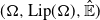 $(\Omega, \mathrm{Lip}(\Omega), \hat{\mathbb E})$
by remembering that
$(\Omega, \mathrm{Lip}(\Omega), \hat{\mathbb E})$
by remembering that $\hat{\mathbb E}$
is the G-expectation on
$\hat{\mathbb E}$
is the G-expectation on $\mathrm{Lip}(\Omega)$
. The reader can refer to [Reference Peng23, Reference Peng24] for more details of G-expectation theory, including the notation of conditional expectation
$\mathrm{Lip}(\Omega)$
. The reader can refer to [Reference Peng23, Reference Peng24] for more details of G-expectation theory, including the notation of conditional expectation $\hat{\mathbb E}[\cdot\mid\Omega_t]$
.
$\hat{\mathbb E}[\cdot\mid\Omega_t]$
.
Lemma 2.1. Let $\overline{\sigma}^2 = \hat{\mathbb E}[B^2_1]$
,
$\overline{\sigma}^2 = \hat{\mathbb E}[B^2_1]$
, $\underline{\sigma}^2 = -\hat{\mathbb E}[\!-B^2_1]$
,
$\underline{\sigma}^2 = -\hat{\mathbb E}[\!-B^2_1]$
, $0 \leq z \leq t <\infty$
, and
$0 \leq z \leq t <\infty$
, and $n \geq 1$
; then
$n \geq 1$
; then
 \begin{align*} \hat{\mathbb E}[(\langle B \rangle_t - \langle B \rangle_z)^n \rvert \Omega_z] & = \overline{\sigma}^{2n} (t-z)^n, \\[2mm] \hat{\mathbb E}[-(\langle B \rangle_t - \langle B \rangle _z)^n\rvert\Omega_z] & = -\underline{\sigma}^{2n} (t-z)^n, \\[2mm] \underline{\sigma}^2 (t-z) \leq \langle B \rangle _t - \langle B \rangle _z & \leq \overline{\sigma}^2 (t-z) \quad {q.s.} \end{align*}
Lemma 2.2. (Borel–Cantelli.) For a sequence of Borel sets $(A_n)_{n \in \mathbb{N}}$
with
$(A_n)_{n \in \mathbb{N}}$
with $\sum_{n=1}^{\infty} c(A_n) < \infty$
,
$\sum_{n=1}^{\infty} c(A_n) < \infty$
, $\limsup_{n \rightarrow \infty}A_n$
is polar.
$\limsup_{n \rightarrow \infty}A_n$
is polar.
We set up the following sets:
-
$L^0(\Omega)$
: the space of all
$\mathcal{B}(\Omega)$
-measurable real functions;
-
$L^0(\Omega_t)$
: the space of all
$\mathcal{B}(\Omega_t)$
-measurable real functions;
-
$B_\mathrm{b}(\Omega)$
: the space of all bounded elements in
$L^0(\Omega)$
;
-
$B_\mathrm{b}(\Omega_t)$
: the space of all bounded elements in
$L^0(\Omega_t)$
;
-
$C_\mathrm{b}(\Omega)$
: all continuous elements in
$B_\mathrm{b}(\Omega)$
;


and, for $p > 0$
,
$p > 0$
,
-
${\mathcal L}^p \, :\!= \, \{X \in L^0(\Omega) \colon \hat{\mathbb E}[|X|^p] = \sup\nolimits_{P \in \mathcal{P}} E_P[|X|^p] < \infty\}$
;
-
${\mathcal N} \, :\!= \, \{X \in L^0(\Omega) \colon X = 0,\ c\mathrm{-}q.s.\}$
.


Lemma 2.3 (Markov’s inequality.) Set ${\mathbb{L}}^p \, :\!= \, {\mathcal L}^p/{\mathcal N}$
. Let
${\mathbb{L}}^p \, :\!= \, {\mathcal L}^p/{\mathcal N}$
. Let $X \in {\mathbb{L}}^p$
for
$X \in {\mathbb{L}}^p$
for $p > 0$
. Then, for each
$p > 0$
. Then, for each $\alpha > 0$
,
$\alpha > 0$
, $c ({\{|X| > \alpha\}}) \leq {\hat{\mathbb E}[|X|^p]}/{\alpha^p}$
.
$c ({\{|X| > \alpha\}}) \leq {\hat{\mathbb E}[|X|^p]}/{\alpha^p}$
.
As indicated in the introduction, the G-Itô integral of a quasi-continuous process was first defined in [Reference Peng24] and the definition was extended to the larger spaces containing the stochastic process without assuming quasi-continuity in [Reference Li and Peng15]. In the following, based on [Reference Li and Peng14, Reference Li and Peng15], we briefly review this.
Let $p > 0$
. We denote by
$p > 0$
. We denote by $L^p_{\star}(\Omega)$
and
$L^p_{\star}(\Omega)$
and $L^p_{\star}(\Omega_t)$
the completion of
$L^p_{\star}(\Omega_t)$
the completion of $B_\mathrm{b}(\Omega)$
and
$B_\mathrm{b}(\Omega)$
and $B_\mathrm{b}(\Omega_t)$
under the norm
$B_\mathrm{b}(\Omega_t)$
under the norm $\|\cdot \|_p$
, respectively. We can prove that
$\|\cdot \|_p$
, respectively. We can prove that $L^p_G(\Omega)$
is the space of the completion of
$L^p_G(\Omega)$
is the space of the completion of $C_\mathrm{b}(\Omega)$
under the natural norm
$C_\mathrm{b}(\Omega)$
under the natural norm $\|\cdot\|_p$
, and
$\|\cdot\|_p$
, and
 \begin{equation*} L^p_{G}(\Omega) = \{X \in L^0(\Omega) \mid X\ \text{has a q.c. version with}\ \textstyle\lim_{n \rightarrow \infty} \hat{\mathbb E}[|X|^pI_{\{|X|>n\}}]=0\}.\end{equation*}
Also, $L^p_{\star}(\Omega) = \{X \in L^0(\Omega) \mid \lim_{n \rightarrow \infty} \hat{\mathbb E}[|X|^pI_{\{|X|>n\}}]=0\}$
. Clearly,
$L^p_{\star}(\Omega) = \{X \in L^0(\Omega) \mid \lim_{n \rightarrow \infty} \hat{\mathbb E}[|X|^pI_{\{|X|>n\}}]=0\}$
. Clearly,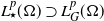 $L^p_{\star}(\Omega) \supset L^p_G(\Omega)$
.
$L^p_{\star}(\Omega) \supset L^p_G(\Omega)$
.
Let $T \in \mathbb{R}^{+}$
. We define the following type of simple process:
$T \in \mathbb{R}^{+}$
. We define the following type of simple process:
 \begin{multline*} M_\mathrm{b,0}(0,T) = \Bigg\{\eta \mid \eta_t(\omega) = \sum_{j=0}^{N-1}\xi_j(\omega)I_{[t_j,t_{j+1})}(t) \\[3pt] \text{for all}\ N \in \mathbb{N}, 0=t_0 < \cdots < t_N = T, \xi_j \in B_\mathrm{b}\big(\Omega_{t_j}\big), j =0,\ldots, N-1\Bigg\}.\end{multline*}
This allows us to define Itô’s integral with respect to G-Brownian motion and its quadratic variation process for functions belonging to $M_\mathrm{b,0}(0,T)$
. From now, we assume that
$M_\mathrm{b,0}(0,T)$
. From now, we assume that $d=1$
. Now, for
$d=1$
. Now, for $\eta \in M_\mathrm{b,0}(0,T)$
, we define
$\eta \in M_\mathrm{b,0}(0,T)$
, we define
 \begin{align*} I(\eta) = \int_0^T\eta_t(\omega)\,{\mathrm{d}} B_t & \, :\!= \, \sum_{j=0}^{N-1} \xi_j(\omega)\big(B_{t_{j+1}} - B_{t_j}\big), \\[3pt]J(\eta) = \int_0^T \eta_t(\omega)\,{\mathrm{d}}\langle B \rangle_t & \, :\!= \, \sum_{j=0}^{N-1} \xi_j(\omega) \big(\langle B \rangle_{t_{j+1}} - \langle B \rangle_{t_j}\big).\end{align*}
Let $p \geq 1$
. We denote by
$p \geq 1$
. We denote by $M^p_{*}(0,T)$
the completion of
$M^p_{*}(0,T)$
the completion of $M_\mathrm{b,0}(0,T)$
under the norm
$M_\mathrm{b,0}(0,T)$
under the norm
 \begin{equation} \|\eta\|_{M^p_{*}(0,T)} \, :\!= \, \bigg\{\hat{\mathbb E}\bigg[\!\int_{0}^{T}|\eta_t|^p\,{\mathrm{d}} t\bigg]\bigg\}^{{1}/{p}}.\end{equation}
The mapping $I \colon M^{b,0}(0,T) \rightarrow L^2_{\star}(\Omega_T)$
is a linear continuous mapping and thus can be continuously extended to
$I \colon M^{b,0}(0,T) \rightarrow L^2_{\star}(\Omega_T)$
is a linear continuous mapping and thus can be continuously extended to $I \colon M^2_{\star}(0,T) \rightarrow L^2_{\star}(\Omega_T)$
. Moreover, for
$I \colon M^2_{\star}(0,T) \rightarrow L^2_{\star}(\Omega_T)$
. Moreover, for $\eta \in M^2_{\star}(0,T)$
,
$\eta \in M^2_{\star}(0,T)$
,
 \begin{align} \hat{\mathbb E}\bigg[\!\int_0^T \eta_v\,{\mathrm{d}} B_v\bigg] =0.\end{align}
Similarly, J can be continuously extended to $J \colon M^1_{\star}(0,T) \rightarrow L^1_{\star}(\Omega_T)$
. Note that
$J \colon M^1_{\star}(0,T) \rightarrow L^1_{\star}(\Omega_T)$
. Note that $M^p_{\star}(0,T) \supset M^q_{\star}(0,T)$
for
$M^p_{\star}(0,T) \supset M^q_{\star}(0,T)$
for $p < q$
. We can show that
$p < q$
. We can show that $\int_0^t\eta_s\,{\mathrm{d}} B_s$
is continuous in t quasi-surely for
$\int_0^t\eta_s\,{\mathrm{d}} B_s$
is continuous in t quasi-surely for $0 \leq t \leq T$
, and also
$0 \leq t \leq T$
, and also $\int_0^.\eta_s\,{\mathrm{d}} B_s \in M^2_{\star}(0,T)$
for any
$\int_0^.\eta_s\,{\mathrm{d}} B_s \in M^2_{\star}(0,T)$
for any $\eta \in M^2_{\star}(0, T)$
.
$\eta \in M^2_{\star}(0, T)$
.
Proposition 2.1. Let $p\geq 1$
,
$p\geq 1$
, $X, \eta \in M_{\star}^p([0, T])$
with
$X, \eta \in M_{\star}^p([0, T])$
with $\eta$
bounded; then
$\eta$
bounded; then $X\eta \in M_{\star}^p([0, T])$
.
$X\eta \in M_{\star}^p([0, T])$
.
Analogously to $M_\mathrm{b,0}(0, T)$
, we define
$M_\mathrm{b,0}(0, T)$
, we define $\bar{M}_\mathrm{b,0}(0, T)$
as the collection of simple processes where
$\bar{M}_\mathrm{b,0}(0, T)$
as the collection of simple processes where $\xi_j \in L^p_G(\Omega_{t_j})$
for
$\xi_j \in L^p_G(\Omega_{t_j})$
for $p \geq 1$
and
$p \geq 1$
and ${M}^p_G(0, T)$
, as the completion of
${M}^p_G(0, T)$
, as the completion of $\bar{M}_\mathrm{b,0}(0, T)$
under the norm
$\bar{M}_\mathrm{b,0}(0, T)$
under the norm $\|\eta\|_{M^p_G(0,T)}$
, which is defined similarly to
$\|\eta\|_{M^p_G(0,T)}$
, which is defined similarly to $\|\cdot\|_{M^p_{*}(0,T)}$
in (2.3).
$\|\cdot\|_{M^p_{*}(0,T)}$
in (2.3).
Definition 2.4. Let $p>0$
be fixed. A stochastic process
$p>0$
be fixed. A stochastic process $(\eta_t)_{t\geq 0}$
is said to be in
$(\eta_t)_{t\geq 0}$
is said to be in $M^p_{\unicode{x03C9}}(0,T)$
if there exists a sequence of increasing stopping times
$M^p_{\unicode{x03C9}}(0,T)$
if there exists a sequence of increasing stopping times $\{\sigma_m\}_{m=1}^{\infty}$
with
$\{\sigma_m\}_{m=1}^{\infty}$
with $\sigma_m \uparrow T$
quasi-surely such that
$\sigma_m \uparrow T$
quasi-surely such that $\eta I_{[0,\sigma_m]} \in M^p_{\star}(0,T)$
and
$\eta I_{[0,\sigma_m]} \in M^p_{\star}(0,T)$
and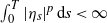 $\int_0^T|\eta_s|^p\,{\mathrm{d}} s < \infty$
, quasi-surely.
$\int_0^T|\eta_s|^p\,{\mathrm{d}} s < \infty$
, quasi-surely.
Let $\mathcal{F}_t \, :\!= \, \mathcal{B}(\Omega_t)$
for
$\mathcal{F}_t \, :\!= \, \mathcal{B}(\Omega_t)$
for $t \geq 0$
. A map
$t \geq 0$
. A map $\tau \colon \Omega \rightarrow [0,T]$
is said to be a stopping time if
$\tau \colon \Omega \rightarrow [0,T]$
is said to be a stopping time if $\{\tau \leq t\} \in \mathcal{F}_t$
. For each stopping time
$\{\tau \leq t\} \in \mathcal{F}_t$
. For each stopping time $\tau$
,
$\tau$
, $p \geq 1$
, and
$p \geq 1$
, and $\eta \in M^p_{\star}(0,T)$
, using Proposition 2.1 we can prove that
$\eta \in M^p_{\star}(0,T)$
, using Proposition 2.1 we can prove that $I_{[0,\tau]}(\! \cdot \!)\eta \in M^p_{\star}(0,T) \subseteq M^p_{\unicode{x03C9}}(0,T)$
. So, the integral
$I_{[0,\tau]}(\! \cdot \!)\eta \in M^p_{\star}(0,T) \subseteq M^p_{\unicode{x03C9}}(0,T)$
. So, the integral $\int_0^t\eta_s\,{\mathrm{d}} B_s$
is well-defined and we have
$\int_0^t\eta_s\,{\mathrm{d}} B_s$
is well-defined and we have
 \begin{equation} \int_0^tI_{[0,\tau]}(s)\eta_s\,{\mathrm{d}} B_s = \int_0^{t \wedge \tau} \eta_s\,{\mathrm{d}} B_s \quad q.s.\end{equation}
Lemma 2.4 ([Reference Li, Lin and Lin13].) Let $\eta \in M^p_{\unicode{x03C9}}([0, T])$
. Then, for
$\eta \in M^p_{\unicode{x03C9}}([0, T])$
. Then, for $p > 0$
, there exists
$p > 0$
, there exists $C_p>0$
depending only on p such that
$C_p>0$
depending only on p such that
 \begin{equation*} \hat{\mathbb E}\bigg[\!\sup\nolimits_{0 \leq s \leq t}\bigg|\int_0^s\eta_v\,{\mathrm{d}} B_v\bigg|^p\bigg] \leq C_p \overline{\sigma}^{p/2}\hat{\mathbb E}\bigg[\bigg(\!\int_0^t |\eta_v|^2\,{\mathrm{d}} v\bigg)^{p/2}\bigg], \end{equation*}
where $\hat{\mathbb E}[B^2_1] = \overline{\sigma}^2$
.
$\hat{\mathbb E}[B^2_1] = \overline{\sigma}^2$
.
3. The G-SDE under locally Lipschitz conditions
In this section we consider the following type of one-dimensional SDE driven by G-Brownian motion:
 \begin{equation} X_t = x_0 + \int_0^t f(X_s)\,{\mathrm{d}} s + \int_0^t g(X_s)\,{\mathrm{d}}\langle B\rangle_s + \int_0^t \sigma(X_s)\,{\mathrm{d}} B_s, \quad t \in [0, T],\end{equation}
where $x_0 \in \mathbb{R}$
and
$x_0 \in \mathbb{R}$
and $f(x), g(x), \sigma(x) \in M^p_{G} ([0,T]) \subset M^p_{\star} ([0,T])$
for any
$f(x), g(x), \sigma(x) \in M^p_{G} ([0,T]) \subset M^p_{\star} ([0,T])$
for any $x \in \mathbb{R}$
and some
$x \in \mathbb{R}$
and some $ p \geq 2$
. Also, for any
$ p \geq 2$
. Also, for any $R > 0$
, the coefficients
$R > 0$
, the coefficients $f, g, \sigma \colon \mathbb{R} \rightarrow \mathbb{R}$
satisfy the assumption
$f, g, \sigma \colon \mathbb{R} \rightarrow \mathbb{R}$
satisfy the assumption
 \begin{align} |b(x) - b(y)| \leq K_R|x-y|\end{align}
for any $x, y \in\mathbb{R}$
with
$x, y \in\mathbb{R}$
with $|x| \vee |y| \leq R$
and some positive constant
$|x| \vee |y| \leq R$
and some positive constant $K_R$
. Note that function b is taken from set
$K_R$
. Note that function b is taken from set $\{f, g, \sigma\}$
. Moreover,
$\{f, g, \sigma\}$
. Moreover,
 \begin{align} xf(x) + xg(x) + |\sigma(x)|^2 \leq K(1 + |x|^2)\end{align}
for any $x\in\mathbb{R}$
and some positive constant K.
$x\in\mathbb{R}$
and some positive constant K.
Definition 3.1. Let $p \geq 2$
. The process
$p \geq 2$
. The process $(X_t)_{t \in [0,T]} \in M^p_{\unicode{x03C9}}([0,T];\, \mathbb{R})$
is said to be the solution of G-SDE (3.1) if it satisfies the equation and has t-continuous paths on [0, T].
$(X_t)_{t \in [0,T]} \in M^p_{\unicode{x03C9}}([0,T];\, \mathbb{R})$
is said to be the solution of G-SDE (3.1) if it satisfies the equation and has t-continuous paths on [0, T].
It is well known that G-SDEs under globally Lipschitz coefficients possess a unique solution. Now, based on [Reference Li, Lin and Lin13, Theorem 4.5 and Example 4.7], we present following theorem which deals with the locally Lipschitz coefficients case.
In the next section we deal with the stability property of the trivial and approximation solutions.
3.1. Stability of the G-SDE
In this section we review the concept of stability of the trivial solution $X \equiv 0 $
of the G-SDE (3.1). To this end, we first assume that
$X \equiv 0 $
of the G-SDE (3.1). To this end, we first assume that
 \begin{align} f(0) = 0, \qquad g(0) = 0, \qquad \sigma(0) = 0.\end{align}
Definition 3.2. Let $X^{s,x}$
be the solution of G-SDE (3.1) starting at s and
$X^{s,x}$
be the solution of G-SDE (3.1) starting at s and $X(s) = x$
,
$X(s) = x$
, $x \in \mathbb{R}$
. Let
$x \in \mathbb{R}$
. Let $p>0$
. If there exist some positive constants C and
$p>0$
. If there exist some positive constants C and $\lambda$
such that
$\lambda$
such that $\hat{\mathbb E}[|X^{s,x}_t|^p] \leq C{|x_0|^p}{\mathrm{e}}^{-\lambda(t-s)}$
, then the trivial solution is called exponentially p-stable. In particular, when
$\hat{\mathbb E}[|X^{s,x}_t|^p] \leq C{|x_0|^p}{\mathrm{e}}^{-\lambda(t-s)}$
, then the trivial solution is called exponentially p-stable. In particular, when $p = 2$
, the trivial solution is said to be asymptotically exponentially stable in mean square. Moreover, the trivial solution of the G-SDE is said to be quasi-surely exponentially stable if there exists a positive
$p = 2$
, the trivial solution is said to be asymptotically exponentially stable in mean square. Moreover, the trivial solution of the G-SDE is said to be quasi-surely exponentially stable if there exists a positive $\eta > 0$
such that
$\eta > 0$
such that $\limsup_{t \rightarrow \infty} \{\log(|X^{s,x}_t|)/{t}\} < -\eta$
q.s.
$\limsup_{t \rightarrow \infty} \{\log(|X^{s,x}_t|)/{t}\} < -\eta$
q.s.
We now present [Reference Li, Lin and Lin13, Corollary 5.6] for the one-dimensional case.
Theorem 3.2. Let $p>0$
. Assume that conditions (3.2) and (3.4) hold, and there exist constants
$p>0$
. Assume that conditions (3.2) and (3.4) hold, and there exist constants $\alpha_1, \alpha_2, \alpha_3 \in \mathbb{R}$
with
$\alpha_1, \alpha_2, \alpha_3 \in \mathbb{R}$
with $0 \leq \alpha_2 < \alpha_3$
such that, for
$0 \leq \alpha_2 < \alpha_3$
such that, for $x \in \mathbb{R}$
,
$x \in \mathbb{R}$
,
 \begin{equation} xf(x)+ G( 2xg(x) + \sigma^2(x)) \leq \alpha_1 x^2, \end{equation}
where the function G is defined by (2.2) and
 \begin{equation} \alpha^2_2 \leq \overline{\sigma}^2 \sigma^2(x) \leq \alpha^2_3 \end{equation}
for any $x \in \mathbb{R}$
. Then, the trivial solution of the G-SDE (3.1) is exponentially p-stable if
$x \in \mathbb{R}$
. Then, the trivial solution of the G-SDE (3.1) is exponentially p-stable if $\alpha_1 <0$
and
$\alpha_1 <0$
and $p < 2+ 2|\alpha_1|/\alpha^2_3$
, or
$p < 2+ 2|\alpha_1|/\alpha^2_3$
, or $0 \leq \alpha_1 \leq \alpha^2_2$
and
$0 \leq \alpha_1 \leq \alpha^2_2$
and $p < 2-2\alpha_1/\alpha^2_2$
.
$p < 2-2\alpha_1/\alpha^2_2$
.
Remark 3.1. In addition to conditions (3.2) and (3.4), let the G-SDE (3.1) satisfy the condition $xf(x) \vee |xg(x)| \vee \sigma^2(x) \leq K|x|^2$
for some
$xf(x) \vee |xg(x)| \vee \sigma^2(x) \leq K|x|^2$
for some $K>0$
and any
$K>0$
and any $x \in \mathbb{R}$
. If the trivial solution of the equation is exponentially p-stable,
$x \in \mathbb{R}$
. If the trivial solution of the equation is exponentially p-stable, $p>0$
, then it is quasi-surely exponentially stable. See [Reference Li, Lin and Lin13, Theorem 5.8].
$p>0$
, then it is quasi-surely exponentially stable. See [Reference Li, Lin and Lin13, Theorem 5.8].
4. A time discretization scheme
In this section we set up a so-called $\theta$
-Euler–Maruyama method (
$\theta$
-Euler–Maruyama method ( $\theta$
-EM for short) to approximate the true solution of the G-SDE (3.1); we then prove that it converges to the exact solution.
$\theta$
-EM for short) to approximate the true solution of the G-SDE (3.1); we then prove that it converges to the exact solution.
Let $n \in \mathbb{N}$
. We consider a time discretization of the interval [0, T] as
$n \in \mathbb{N}$
. We consider a time discretization of the interval [0, T] as $0 = t^n_0 < \cdots < t^n_{N_n} = T$
, with the time steps
$0 = t^n_0 < \cdots < t^n_{N_n} = T$
, with the time steps $\Delta_i = t^n_{i+1} - t^n_i$
for
$\Delta_i = t^n_{i+1} - t^n_i$
for $i=0,\ldots,N_n-1$
. We denote by
$i=0,\ldots,N_n-1$
. We denote by $\widetilde{Y}$
the numerical solution
$\widetilde{Y}$
the numerical solution $\theta$
-EM obtained by the scheme
$\theta$
-EM obtained by the scheme
 \begin{equation}\widetilde{Y}_{i+1} = \widetilde{Y}_i + (1-\theta)f(\widetilde{Y}_i)\Delta_i + \theta f(\widetilde{Y}_{i+1})\Delta_i + g(\widetilde{Y}_i)\,\Delta\langle B\rangle_i + \sigma(\widetilde{Y}_i)\,\Delta B_i\end{equation}
for $i = 0,1,\ldots,{N_n}-1$
, where
$i = 0,1,\ldots,{N_n}-1$
, where $\theta \in [0,1]$
,
$\theta \in [0,1]$
, $\widetilde{Y}_{0} = x$
,
$\widetilde{Y}_{0} = x$
, $\Delta \langle B\rangle_i = \langle B \rangle_{t_{i+1}} - \langle B \rangle_{t_i}$
, and
$\Delta \langle B\rangle_i = \langle B \rangle_{t_{i+1}} - \langle B \rangle_{t_i}$
, and $\Delta B_i = B_{t_{i+1}} - B_{t_i}$
. Note that
$\Delta B_i = B_{t_{i+1}} - B_{t_i}$
. Note that $\theta \in [0, 1]$
controls the degree of implicitness of the scheme.
$\theta \in [0, 1]$
controls the degree of implicitness of the scheme.
Let $t \in [0, T]$
. Now, we define a continuous-time approximation of the scheme (4.1) as
$t \in [0, T]$
. Now, we define a continuous-time approximation of the scheme (4.1) as
 \begin{align} \widetilde{Y}^n(t) & = \widetilde{Y}_0 + (1-\theta)\int_{0}^{t}f(\widetilde{Y}_{{\lfloor s \rfloor}})\,{\mathrm{d}} s + \theta\int_{0}^{t}f(\widetilde{Y}_{{\lceil s \rceil}})\,{\mathrm{d}} s \nonumber \\[3pt] & \quad + \int_{0}^{t}g(\widetilde{Y}_{{\lfloor s \rfloor}})\,{\mathrm{d}}\langle B\rangle_s + \int_{0}^{t}\sigma(\widetilde{Y}_{{\lfloor s \rfloor}})\,{\mathrm{d}} B(s),\end{align}
where $\lfloor s \rfloor \, :\!= \, i$
and
$\lfloor s \rfloor \, :\!= \, i$
and $\lceil s \rceil \, :\!= \, i+1 $
for
$\lceil s \rceil \, :\!= \, i+1 $
for $ t_i \leq s < t_{i+1};$
we set
$ t_i \leq s < t_{i+1};$
we set $\lfloor N_n \rfloor \, :\!= \, N_n$
and
$\lfloor N_n \rfloor \, :\!= \, N_n$
and $\lceil N_n \rceil \, :\!= \, N_n$
as a convenience. Note that the process
$\lceil N_n \rceil \, :\!= \, N_n$
as a convenience. Note that the process $(\widetilde{Y}^n(t))_{\{t \in [0,T]\}} \in M^p_{\unicode{x03C9}}([0,T];\, \mathbb{R})$
.
$(\widetilde{Y}^n(t))_{\{t \in [0,T]\}} \in M^p_{\unicode{x03C9}}([0,T];\, \mathbb{R})$
.
In the following we investigate the convergence of the discretization scheme (4.2) in the pth mean for $p \geq 1$
. To this end, inspired by Lemma 2.1, we present following remark.
$p \geq 1$
. To this end, inspired by Lemma 2.1, we present following remark.
Remark 4.1. Let $p>0$
and
$p>0$
and $\eta \in M^p_{\unicode{x03C9}}([0, T];\, \mathbb{R})$
. Then
$\eta \in M^p_{\unicode{x03C9}}([0, T];\, \mathbb{R})$
. Then
 \begin{equation*} \hat{\mathbb E}\bigg[\!\sup\nolimits_{0 \leq s \leq t}\bigg|\int_0^s\eta_v\,{\mathrm{d}}\langle B\rangle_v\bigg|^p\bigg] \leq \overline{\sigma}^{2p}t^{p-1}\hat{\mathbb E}\bigg[\!\int_0^t|\eta_v|^p\,{\mathrm{d}} v\bigg] \end{equation*}
for any $t \in [0, T]$
.
$t \in [0, T]$
.
We assume that for $p \geq 2$
, there exists a constant A such that
$p \geq 2$
, there exists a constant A such that
 \begin{equation} \hat{\mathbb E}(\!\sup\nolimits_{0 \leq t \leq T} |X(t)|^p) \vee \hat{\mathbb E}(\!\sup\nolimits_{0 \leq t \leq T} |\widetilde{Y}^n(t)|^p) \leq A.\end{equation}
This assumption does not pose a limitation. For example, the relation (4.6) stated in Theorem 4.2 ensures that (4.3) holds true.
Now, we present Young’s inequality before investigating the convergence of the numerical scheme.
Lemma 4.1 (Young’s inequality.) For ${1}/{r}+{1}/{q}=1$
,
${1}/{r}+{1}/{q}=1$
,
 \begin{equation*} ab \leq \frac{\delta}{r} a^r + \frac{1}{q \delta^{{q}/{r}}}b^q \quad \text{for all}\ a, b, \delta > 0. \end{equation*}
Now let $R>0$
. Set
$R>0$
. Set $\tau_R \, :\!= \, \inf\{t \geq 0 \colon |\widetilde{Y}^n(t)|\geq R\}$
,
$\tau_R \, :\!= \, \inf\{t \geq 0 \colon |\widetilde{Y}^n(t)|\geq R\}$
, $\rho_R \, :\!= \, \inf\{t \geq 0 \colon |X(t)|\geq R\}$
, and
$\rho_R \, :\!= \, \inf\{t \geq 0 \colon |X(t)|\geq R\}$
, and $\gamma_R\, :\!= \,\tau_R \wedge \rho_R$
.
$\gamma_R\, :\!= \,\tau_R \wedge \rho_R$
.
Lemma 4.2. Assume that $R>0$
and
$R>0$
and $t \in [t_i, t_{i+1}] \subseteq [0, T \wedge \gamma_R]$
for some
$t \in [t_i, t_{i+1}] \subseteq [0, T \wedge \gamma_R]$
for some $i \in \{0,\ldots,N_n-1\}$
. Let assumption (3.2) hold. Then, there exists a positive constant
$i \in \{0,\ldots,N_n-1\}$
. Let assumption (3.2) hold. Then, there exists a positive constant $\bar{c}$
depending on
$\bar{c}$
depending on $K_R$
,
$K_R$
, $C_2$
,
$C_2$
, $\overline{\sigma}$
, T, A, f(0), g(0), and h(0) such that
$\overline{\sigma}$
, T, A, f(0), g(0), and h(0) such that
 \begin{align*} \hat{\mathbb E}[|\widetilde{Y}^n(t) - \widetilde{Y}_{i}|^2] & \leq \bar{c}(t - t_i), \\[1mm] \hat{\mathbb E}[|\widetilde{Y}^n(t) - \widetilde{Y}_{i+1}|^2] & \leq \bar{c}(t_{i+1} - t). \end{align*}
Proof. According to (4.2), we can write
 \begin{align*} \widetilde{Y}^n(t) & = \widetilde{Y}_i + \theta\int_{t_i}^{t}f(\widetilde{Y}_{{\lfloor s \rfloor}})\,{\mathrm{d}} s + (1-\theta)\int_{t_i}^{t}f(\widetilde{Y}_{{\lceil s \rceil}})\,{\mathrm{d}} s \\[3pt] & \quad + \int_{t_i}^{t}g(\widetilde{Y}_{{\lfloor s \rfloor}})\,{\mathrm{d}}\langle B\rangle_s + \int_{t_i}^{t}\sigma(\widetilde{Y}_{{\lfloor s \rfloor}})\,{\mathrm{d}} B(s). \end{align*}
Using Hölder’s inequality, Lemma 2.4, and Remark 4.1 results in
 \begin{align*} \hat{\mathbb E}[|\widetilde{Y}^n(t) - \widetilde{Y}_i|^2] & \leq 4\theta^2(t-t_i)\int_{t_i}^{t}\hat{\mathbb E}[|f(\widetilde{Y}_{{\lfloor s \rfloor}})|^2]\,{\mathrm{d}} s \\[3pt] & \quad + 4(1-\theta)^2(t-t_i)\int_{t_i}^{t}\hat{\mathbb E}[|f(\widetilde{Y}_{{\lceil s \rceil}})|^2]\,{\mathrm{d}} s \\[3pt] & \quad + 4\overline{\sigma}^4(t-t_i) \int_{t_i}^{t}\hat{\mathbb E}[|g(\widetilde{Y}_{{\lfloor s\rfloor}})|^2]\,{\mathrm{d}} s + 4C_2\overline{\sigma}\int_{t_i}^{t}\hat{\mathbb E}[|\sigma(\widetilde{Y}_{{\lfloor s \rfloor}})|^2]\,{\mathrm{d}} s. \end{align*}
Since $[t, t_{i+1}] \subseteq [0, T \wedge \gamma_R]$
, by the locally Lipschitz property (3.2) and assumption (4.3), we can see that
$[t, t_{i+1}] \subseteq [0, T \wedge \gamma_R]$
, by the locally Lipschitz property (3.2) and assumption (4.3), we can see that
 \begin{equation*} \hat{\mathbb E}[|b(\widetilde{Y}_{{\lfloor s \rfloor}})|^2] \leq 2|b(0)|^2 + 2K^2_R \hat{\mathbb E} (\!\sup\nolimits_{0 \leq s \leq T} |\widetilde{Y}^n(s)|^2) \leq 2|b(0)|^2 + 2K^2_R A \end{equation*}
for $b \in \{f,g,h\}$
. Then,
$b \in \{f,g,h\}$
. Then, $\hat{\mathbb E}[|\widetilde{Y}^n(t) - \widetilde{Y}_i|^2] \leq 8(K^2_R A + M_{f,g,h})(T(2 + \overline{\sigma}^4) + C_2\overline{\sigma})(t-t_i)$
, where
$\hat{\mathbb E}[|\widetilde{Y}^n(t) - \widetilde{Y}_i|^2] \leq 8(K^2_R A + M_{f,g,h})(T(2 + \overline{\sigma}^4) + C_2\overline{\sigma})(t-t_i)$
, where $M_{f,g,h} = \max\{|f(0)|^2, |g(0)|^2, |h(0)|^2\}$
and the second assertion follows.
$M_{f,g,h} = \max\{|f(0)|^2, |g(0)|^2, |h(0)|^2\}$
and the second assertion follows.
Theorem 4.1. Let $n \in \mathbb{N}$
and set
$n \in \mathbb{N}$
and set $e_n(t) \, :\!= \, X(t) - \widetilde{Y}^n(t)$
for
$e_n(t) \, :\!= \, X(t) - \widetilde{Y}^n(t)$
for $t \in [0, T]$
. Then the continuous scheme (4.2) converges to the true solution of (3.1) in the sense
$t \in [0, T]$
. Then the continuous scheme (4.2) converges to the true solution of (3.1) in the sense
 \begin{equation*} \lim_{h_n \rightarrow 0} \hat{\mathbb E}(\!\sup\nolimits_{0 \leq t \leq T} |e_n(t)|^2) = 0, \end{equation*}
where $h_n = \sup\nolimits_{0 \leq i \leq {N_n}-1} |t^n_{i+1}-t^n_i|$
.
$h_n = \sup\nolimits_{0 \leq i \leq {N_n}-1} |t^n_{i+1}-t^n_i|$
.
Proof. For any $t \in [0, T]$
, we have that
$t \in [0, T]$
, we have that
 \begin{equation*} \hat{\mathbb E}(\!\sup\nolimits_{0 \leq v \leq t} |e_n(v)|^2) \leq \hat{\mathbb E}(\!\sup\nolimits_{0 \leq v \leq t} |e_n(v)|^2\mathbf{1}_{\{\gamma_R > T\}}) + \hat{\mathbb E}(\!\sup\nolimits_{0 \leq v \leq t} |e_n(v)|^2\mathbf{1}_{\{\gamma_R \leq T\}}). \end{equation*}
Applying Lemma 4.1 for the second term by setting $r={p}/{2}$
and
$r={p}/{2}$
and $q={p}/({p-2})$
for
$q={p}/({p-2})$
for $p > 2$
, we arrive at
$p > 2$
, we arrive at
 \begin{align*} \hat{\mathbb E}(\!\sup\nolimits_{0 \leq v \leq t} |e_n(v)|^2) & \leq \hat{\mathbb E}(\!\sup\nolimits_{0 \leq v \leq t} |e_n(v)|^2\mathbf{1}_{\{\gamma_R > T\}}) + \frac{2\delta}{p}\hat{\mathbb E}(\!\sup\nolimits_{0 \leq v \leq t} |e_n(v)|^p) \\[3pt] & \quad + \frac{1-({2}/{p})}{\delta^{{2}/({p-2})}}\hat{\mathbb E}\big(\mathbf{1}_{\{\gamma_R \leq T\}}\big). \end{align*}
According to (4.3), we see that $\hat{\mathbb E}(\!\sup\nolimits_{0 \leq v \leq t} |e_n(v)|^p) \leq 2^pA$
and
$\hat{\mathbb E}(\!\sup\nolimits_{0 \leq v \leq t} |e_n(v)|^p) \leq 2^pA$
and
 \begin{align*} \hat{\mathbb E}\big(\mathbf{1}_{[\gamma_R \leq T]}\big) & \leq {c}(\tau_R \leq T) + {c}(\rho_R \leq T) \\[3pt] & = \hat{\mathbb E}\bigg(\mathbf{1}_{\{\tau_R \leq T\}}\frac{|\widetilde{Y}^n(\tau_R)|^p}{R^p}\bigg) + \hat{\mathbb E}\bigg(\mathbf{1}_{\{\rho_R \leq T\}}\frac{|X(\rho_R)|^p}{R^p}\bigg) \\[3pt] & \leq \frac{1}{R^p}\big(\hat{\mathbb E}(\!\sup\nolimits_{0 \leq t \leq T}|\widetilde{Y}^n(t)|^p) + \hat{\mathbb E}(\!\sup\nolimits_{0 \leq t \leq T}|X(t)|^p)\big) \leq \frac{2A}{R^p}. \end{align*}
Finally,
 \begin{equation} \hat{\mathbb E}(\!\sup\nolimits_{0 \leq v \leq t} |e_n(v)|^2) \leq \hat{\mathbb E}(\!\sup\nolimits_{0 \leq v \leq t} |e_n(v \wedge \gamma_R)|^2) + A\bigg(\frac{2^{p+1}\delta}{p} + \frac{2(1-({2}/{p}))}{R^p\delta^{{2}/({p-2})}}\bigg). \end{equation}
Note that by the time evolution of X and $\widetilde{Y}^n$
in (3.1) and (4.2),
$\widetilde{Y}^n$
in (3.1) and (4.2),
 \begin{align*} e_n(v \wedge \gamma_R) & = \theta\int_{0}^{v \wedge \gamma_R}f(X(s))\,{\mathrm{d}} s + (1-\theta)\int_{0}^{v \wedge \gamma_R}f(X(s))\,{\mathrm{d}} s \\[4pt] & \quad + \int_{0}^{v \wedge \gamma_R}g(X(s))\,{\mathrm{d}}\langle B\rangle_s + \int_{0}^{v \wedge \gamma_R}\sigma(X(s))\,{\mathrm{d}} B(s) \\[4pt] & \quad - \theta\int_{0}^{v \wedge \gamma_R}f(\widetilde{Y}_{{\lfloor s \rfloor}})\,{\mathrm{d}} s - (1-\theta)\int_{0}^{v \wedge \gamma_R}f(\widetilde{Y}_{{\lceil s \rceil}})\,{\mathrm{d}} s \\[4pt] & \quad - \int_{0}^{v \wedge \gamma_R}g(\widetilde{Y}_{{\lfloor s \rfloor}})\,{\mathrm{d}}\langle B\rangle_s - \int_{0}^{v \wedge \gamma_R}\sigma(\widetilde{Y}_{{\lfloor s \rfloor}})\,{\mathrm{d}} B(s) \end{align*}
for any $v \leq t$
. Due to
$v \leq t$
. Due to $(a+b+c+d)^2 \leq 4(a^2+b^2+c^2+d^2)$
and by remembering (2.5), we have
$(a+b+c+d)^2 \leq 4(a^2+b^2+c^2+d^2)$
and by remembering (2.5), we have
 \begin{align*} \hat{\mathbb E}(\!\sup\nolimits_{0 \leq v \leq t} |e_n(v \wedge \gamma_R)|^2) & \leq 4\theta^2\,\hat{\mathbb E}\bigg(\!\sup\nolimits_{0 \leq v \leq t}\bigg| \int_{0}^{v}(f(X(s)) - f(\widetilde{Y}_{{\lfloor s \rfloor}}))\mathbf{1}_{[0, v \wedge \gamma_R]}(s)\, {\mathrm{d}} s\bigg|^2\bigg) \\[3pt] & \quad + 4(1-\theta)^2\,\hat{\mathbb E}\bigg(\!\sup\nolimits_{0 \leq v \leq t}\bigg| \int_{0}^{v}(f(X(s)) - f(\widetilde{Y}_{{\lceil s \rceil}}))\mathbf{1}_{[0, v \wedge \gamma_R]}(s)\, {\mathrm{d}} s\bigg|^2\bigg) \\[1mm] & \quad + 4\hat{\mathbb E}\bigg(\!\sup\nolimits_{0 \leq v \leq t}\bigg| \int_{0}^{v}(g(X(s)) - g(\widetilde{Y}_{{\lfloor s \rfloor}}))\mathbf{1}_{[0, v \wedge \gamma_R]}(s)\, {\mathrm{d}}\langle B\rangle_s\bigg|^2\bigg) \\[1mm] & \quad + 4\hat{\mathbb E}\bigg(\!\sup\nolimits_{0 \leq v \leq t}\bigg| \int_{0}^{v}(\sigma(X(s)) - \sigma(\widetilde{Y}_{{\lfloor s \rfloor}}))\mathrm{1}_{[0, v \wedge \gamma_R]}(s)\, {\mathrm{d}} B(s)\bigg|^2\bigg). \end{align*}
Remebering that $\theta \in [0, 1]$
, the Hölder inequality, Lemma 2.4, and Remark 4.1 lead to
$\theta \in [0, 1]$
, the Hölder inequality, Lemma 2.4, and Remark 4.1 lead to
 \begin{align*} \hat{\mathbb E}(\!\sup\nolimits_{0 \leq v \leq t} |e_n(v \wedge \gamma_R)|^2) & \leq 4\bigg(t\int_{0}^{t}\hat{\mathbb E}(|(f(X(s)) - f(\widetilde{Y}_{{\lfloor s \rfloor}}))\mathbf{1}_{[0, t \wedge \gamma_R]}(s)|^2)\,{\mathrm{d}} s \\[1mm] & \quad + t\int_{0}^{t}\hat{\mathbb E}(|(f(X(s)) - f(\widetilde{Y}_{{\lceil s \rceil}}))\mathbf{1}_{[0, t \wedge \gamma_R]}(s)|^2)\,{\mathrm{d}} s \\[1mm] & \quad + t\overline{\sigma}^4\int_{0}^{t}\hat{\mathbb E}(|(g(X(s)) - g(\widetilde{Y}_{{\lfloor s \rfloor}}))\mathbf{1}_{[0, t \wedge \gamma_R]}(s)|^2)\,{\mathrm{d}} s \\[1mm] & \quad + C_2\overline{\sigma}\int_{0}^{t}\hat{\mathbb E}(|(\sigma(X(s)) - \sigma(\widetilde{Y}_{{\lfloor s \rfloor}}))\mathbf{1}_{[0, t \wedge \gamma_R]}(s)|^2)\,{\mathrm{d}} s\bigg). \end{align*}
Due to the local Lipschitz condition (3.2), we get
 \begin{align*} \hat{\mathbb E}(\!\sup\nolimits_{0 \leq v \leq t} |e_n(v \wedge \gamma_R)|^2) & \leq M_R\int_{0}^{t}\hat{\mathbb E}[|X(s) - \widetilde{Y}_{{\lfloor s \rfloor}}|^2\mathbf{1}_{[0, t \wedge \gamma_R]}(s)]\,{\mathrm{d}} s \\[3pt] & \quad + 4TK^2_R\int_{0}^{t}\hat{\mathbb E}[|X(s) - \widetilde{Y}_{{\lceil s \rceil}}|^2\mathbf{1}_{[0, t \wedge \gamma_R]}(s)]\,{\mathrm{d}} s \\[3pt] & \leq \big(2M_R+8TK^2_R\big)\int_{0}^{t}\hat{\mathbb E}[|X(s) - \widetilde{Y}^n(s)|^2\mathbf{1}_{[0, t \wedge \gamma_R]}(s)]\,{\mathrm{d}} s \\[3pt] & \quad + 2M_R\int_{0}^{t}\hat{\mathbb E}[|\widetilde{Y}^n(s) - \widetilde{Y}_{{\lfloor s \rfloor}}|^2\mathbf{1}_{[0, t \wedge \gamma_R]}(s)]\,{\mathrm{d}} s \\[3pt] & \quad + 8TK^2_R\int_{0}^{t}\hat{\mathbb E}[|\widetilde{Y}^n(s) - \widetilde{Y}_{{\lceil s \rceil}}|^2\mathbf{1}_{[0, t \wedge \gamma_R]}(s)]\,{\mathrm{d}} s \\[3pt] & \leq (2M_R+8TK^2_R)\int_{0}^{t}\hat{\mathbb E}[|e_n(s \wedge \gamma_R)|^2]\,{\mathrm{d}} s \\[3pt] & \quad + 2M_R\sum_{i=0}^{N_n-1}\int_{t_i}^{t_{i+1}}\hat{\mathbb E}[|\widetilde{Y}^n(s) - \widetilde{Y}_{i}|^2\mathbf{1}_{[0, t \wedge \gamma_R]}(s)]\,{\mathrm{d}} s \\[3pt] & \quad + 8TK^2_R\sum_{i=0}^{N_n-1}\int_{t_i}^{t_{i+1}}\hat{\mathbb E}[|\widetilde{Y}^n(s) - \widetilde{Y}_{i+1}|^2\mathbf{1}_{[0, t \wedge \gamma_R]}(s)]\,{\mathrm{d}} s, \end{align*}
where $M_R = 4K^2_R (T + T\overline{\sigma}^4 + C_2 \overline{\sigma} )$
. By Lemma 4.2, we get
$M_R = 4K^2_R (T + T\overline{\sigma}^4 + C_2 \overline{\sigma} )$
. By Lemma 4.2, we get
 \begin{align*} \hat{\mathbb E}(\!\sup\nolimits_{0 \leq v \leq t} |e_n(v \wedge \gamma_R)|^2) & \leq \big(2M_R+8TK^2_R\big)\int_{0}^{t}\hat{\mathbb E}(|e_n(s \wedge \gamma_R)|^2)\,{\mathrm{d}} s \\[3pt] & + 2M_R \bar{c}\sum_{i=0}^{N_n-1}\int_{t_i}^{t_{i+1}}(s-t_i)\,{\mathrm{d}} s + 8TK^2_R\bar{c}\sum_{i=0}^{N_n-1}\int_{t_i}^{t_{i+1}}(t_{i+1}-s)\,{\mathrm{d}} s \\[3pt] & \leq \big(2M_R+8TK^2_R\big)\int_{0}^{t}\hat{\mathbb E}(|e_n(s \wedge \gamma_R)|^2)\,{\mathrm{d}} s \\[3pt] & \quad + \bar{c}\big(M_R+4TK^2_R\big)\sum_{i=0}^{N_n-1} {\Delta t_i}^2. \end{align*}
Note that, for simplicity, the points $t^n_{i}$
have been replaced by
$t^n_{i}$
have been replaced by $t_{i}$
for
$t_{i}$
for $i=0,1,\ldots,{N_n}$
. Since
$i=0,1,\ldots,{N_n}$
. Since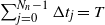 $\sum _ {j=0}^{N_n-1}{\Delta t_j}= T$
,
$\sum _ {j=0}^{N_n-1}{\Delta t_j}= T$
, $\sum_{j=0}^{N_n-1} {\Delta t_j}^2 \leq h_nT$
and, using Grönwall’s lemma, we get
$\sum_{j=0}^{N_n-1} {\Delta t_j}^2 \leq h_nT$
and, using Grönwall’s lemma, we get
 \begin{equation*} \hat{\mathbb E}(\!\sup\nolimits_{0 \leq v \leq t} |e_n(v \wedge \gamma_R)|^p) \leq \bar{c}m_R T{\mathrm{e}}^{2m_RT}h_n, \end{equation*}
where $m_R = M_R+4TK^2_R$
. Now, we return to (4.4). We have
$m_R = M_R+4TK^2_R$
. Now, we return to (4.4). We have
 \begin{equation} \hat{\mathbb E}(\!\sup\nolimits_{0 \leq v \leq t} |e_n(v)|^2) \leq \bar{c}m_RT{\mathrm{e}}^{2m_RT}h_n + A\bigg(\frac{2^{p+1}\delta}{p}+ \frac{2(1-({2}/{p}))}{R^p\delta^{{2}/({p-2})}}\bigg), \end{equation}
and we can choose the step sizes and the parameters $\delta$
and R such that
$\delta$
and R such that
 \begin{equation*} \bar{c}m_RT{\mathrm{e}}^{2m_RT}h_n < \frac{\varepsilon}{3}, \qquad \frac{2^{p+1}\delta A}{p} < \frac{\varepsilon}{3}, \qquad \frac{2(1-({2}/{p}))A}{R^p\delta^{{2}/({p-2})}} < \frac{\varepsilon}{3}; \end{equation*}
then the desired assertion follows.
Remark 4.2. In light of (4.5), taking $\delta = h_n$
and
$\delta = h_n$
and $R = h_n^{{-1}/({p-2})}$
yields the estimate
$R = h_n^{{-1}/({p-2})}$
yields the estimate
 \begin{equation*} \hat{\mathbb E}(\!\sup\nolimits_{0 \leq v \leq t} |e_n(v)|^2) \leq ch_n \end{equation*}
for some positive constant c. This implies that the proposed scheme achieves a global mean-square convergence order proportional to $h_n^{{1}/{2}}$
.
$h_n^{{1}/{2}}$
.
4.1. Numerical stability
In this section we aim to inspect the numerical stability characteristics of the scheme (4.1) in the exponentially mean-square and quasi-sure senses as the value of T approaches infinity. It is important to note that the approximation is not limited to a bounded interval. To this end, we start with the following definitions.
Definition 4.1. A numerical scheme $\{\widetilde{Y}_i\}_{i \in \mathbb{N}}$
applied for approximating G-SDE (3.1) with the initial value
$\{\widetilde{Y}_i\}_{i \in \mathbb{N}}$
applied for approximating G-SDE (3.1) with the initial value $x_0$
is called exponentially p-stable if there exist positive constants C,
$x_0$
is called exponentially p-stable if there exist positive constants C, $\lambda$
, and
$\lambda$
, and $\Delta_0$
such that, for any
$\Delta_0$
such that, for any $i \in \mathbb{N}$
,
$i \in \mathbb{N}$
, $\Delta_i \in (0, \Delta_0)$
and
$\Delta_i \in (0, \Delta_0)$
and $\hat{\mathbb E}[|\widetilde{Y}_i|^p] \leq C\hat{\mathbb E}[|x_0|^p]{\mathrm{e}}^{-\lambda i \Delta^{*}}$
for some
$\hat{\mathbb E}[|\widetilde{Y}_i|^p] \leq C\hat{\mathbb E}[|x_0|^p]{\mathrm{e}}^{-\lambda i \Delta^{*}}$
for some $\Delta^{*} \in (0,\Delta_0)$
.
$\Delta^{*} \in (0,\Delta_0)$
.
Definition 4.2. A numerical scheme $\{\widetilde{Y}_i\}_{i \in \mathbb{N}}$
applied for approximating G-SDE (3.1) with the initial value
$\{\widetilde{Y}_i\}_{i \in \mathbb{N}}$
applied for approximating G-SDE (3.1) with the initial value $x_0$
is called quasi-surely exponentially stable if there exist positive constants
$x_0$
is called quasi-surely exponentially stable if there exist positive constants $\lambda$
and
$\lambda$
and $\Delta_0$
such that, for any
$\Delta_0$
such that, for any $i \in \mathbb{N}$
,
$i \in \mathbb{N}$
, $\Delta_i \in (0, \Delta_0)$
and
$\Delta_i \in (0, \Delta_0)$
and $\limsup_{i \rightarrow \infty} \{\log(|\widetilde{Y}_i|)/i\Delta_i\} < -\lambda$
q.s.
$\limsup_{i \rightarrow \infty} \{\log(|\widetilde{Y}_i|)/i\Delta_i\} < -\lambda$
q.s.
Theorem 4.2. Let assumption (3.2) and the necessary assumptions in Theorem 3.2 hold. If
 \begin{equation} |f(x)| \vee |g(x)| \leq \hat{c}|x| \end{equation}
for any $x \in \mathbb{R}$
and some
$x \in \mathbb{R}$
and some $\hat{c}>0$
, and
$\hat{c}>0$
, and
 \begin{equation} 2\alpha_1 < -\bigg(k\frac{\alpha^2_3}{\overline{\sigma}} + {\overline{\sigma}} (1+\hat{c}^2)\bigg), \end{equation}
where k is a sufficiently large positive constant and
 \begin{equation} \begin{cases} \hphantom{-}16\hat{c}(\beta - 4\hat{c}(1+{\overline{\sigma}}^4)) < -c_1-c_2-c_3, \\[2pt] -16\hat{c}(\beta + 4\hat{c}(1+{\overline{\sigma}}^4)) < -c_1-c_2+c_3, \end{cases} \end{equation}
where $c_1=(1-2\alpha_1)^2$
,
$c_1=(1-2\alpha_1)^2$
, $c_2=64\hat{c}^2$
,
$c_2=64\hat{c}^2$
, $c_3=16\hat{c}(1-2\alpha_1)$
, and
$c_3=16\hat{c}(1-2\alpha_1)$
, and
 $$\beta = 4C_2\frac{\alpha^2_3}{\overline{\sigma}} + (1+\hat{c}^2)\overline{\sigma}^2+ 2\alpha_1.$$
Then the proposed scheme (4.1) is conditionally asymptotically mean-square stable.
Proof. Taking the square of both sides of (4.1) yields
 \begin{align} \widetilde{Y}_{i+1}^2 & \leq \widetilde{Y}_{i}^2 + 4\big((1-\theta)^2f^2(\widetilde{Y}_i)\Delta_i^2 + \theta^2f^2(\widetilde{Y}_{i+1})\Delta_i^2 + g^2(\widetilde{Y}_i)(\Delta\langle B\rangle_i)^2 + \sigma^2(\widetilde{Y}_i)(\Delta B_i)^2\big) \nonumber \\[2mm] & \quad + 2(1-\theta)\widetilde{Y}_if(\widetilde{Y}_i)\Delta_i + 2\theta\widetilde{Y}_if(\widetilde{Y}_{i+1})\Delta_i + 2\widetilde{Y}_ig(\widetilde{Y}_i)\Delta\langle B\rangle_i + 2\widetilde{Y}_i\sigma(\widetilde{Y}_i)\Delta B_i \end{align}
for $i=0,1,\ldots,N_n-1$
. By adding and subtracting
$i=0,1,\ldots,N_n-1$
. By adding and subtracting $2(1-\theta)G(2\widetilde{Y}_ig(\widetilde{Y}_i) + \sigma^2(\widetilde{Y}_i))\Delta_i$
on the right-hand side of (4.9), we have
$2(1-\theta)G(2\widetilde{Y}_ig(\widetilde{Y}_i) + \sigma^2(\widetilde{Y}_i))\Delta_i$
on the right-hand side of (4.9), we have
 \begin{align} \widetilde{Y}_{i+1}^2 & \leq \widetilde{Y}_{i}^2 + 4\big((1-\theta)^2g^2(\widetilde{Y}_i)\Delta_i^2 + \theta^2f^2(\widetilde{Y}_{i+1})\Delta_i^2 + g^2(\widetilde{Y}_i)(\Delta\langle B\rangle_i)^2 + \sigma^2(\widetilde{Y}_i)(\Delta B_i)^2\big) \nonumber \\[3pt] & \quad + I_1 + I_2 + 2\widetilde{Y}_i\sigma(\widetilde{Y}_i)\Delta B_i, \end{align}
where
 \begin{align*} I_1 & = 2(1-\theta)\big(\widetilde{Y}_i f(\widetilde{Y}_i) + G(2\widetilde{Y}_ig(\widetilde{Y}_i) + \sigma^2(\widetilde{Y}_i))\big)\Delta_i, \\[2mm] I_2 & = -2(1-\theta)G(2\widetilde{Y}_ig(\widetilde{Y}_i) + \sigma^2(\widetilde{Y}_i))\Delta_i + 2\theta\widetilde{Y}_if(\widetilde{Y}_{i+1})\Delta_i + 2\widetilde{Y}_ig(\widetilde{Y}_i)\Delta\langle B\rangle_i. \end{align*}
By (3.5) we get $I_1 \leq 2(1-\theta)\alpha_1 \widetilde{Y}^2_i \Delta_i$
. By considering the two cases
$I_1 \leq 2(1-\theta)\alpha_1 \widetilde{Y}^2_i \Delta_i$
. By considering the two cases $2\widetilde{Y}_ig(\widetilde{Y}_i) + \sigma^2(\widetilde{Y}_i)>0$
and
$2\widetilde{Y}_ig(\widetilde{Y}_i) + \sigma^2(\widetilde{Y}_i)>0$
and $2\widetilde{Y}_ig(\widetilde{Y}_i) + \sigma^2(\widetilde{Y}_i)<0$
and relation (4.6), and using the inequality
$2\widetilde{Y}_ig(\widetilde{Y}_i) + \sigma^2(\widetilde{Y}_i)<0$
and relation (4.6), and using the inequality $2ab \leq a^2+b^2$
, we get
$2ab \leq a^2+b^2$
, we get $I_2 \leq ((1+\hat{c}^2)\overline{\sigma}^2 + \theta)\widetilde{Y}^2_i\Delta_i + \theta\hat{c}^2\widetilde{Y}^2_{i+1}\Delta_i$
. By applying
$I_2 \leq ((1+\hat{c}^2)\overline{\sigma}^2 + \theta)\widetilde{Y}^2_i\Delta_i + \theta\hat{c}^2\widetilde{Y}^2_{i+1}\Delta_i$
. By applying $\hat{\mathbb E}$
on both sides of (4.10), we get
$\hat{\mathbb E}$
on both sides of (4.10), we get
 \begin{align*} & \hat{\mathbb E}\big[\widetilde{Y}_{i+1}^2\big] \\[3pt] & \leq \hat{\mathbb E}\big[\widetilde{Y}_{i}^2\big] \\[3pt] & \quad + 4\big((1-\theta)^2\hat{\mathbb E}[g^2(\widetilde{Y}_i)]\Delta_i^2 + \theta^2\hat{\mathbb E}[f^2(\widetilde{Y}_{i+1})]\Delta_i^2 + \hat{\mathbb E}[g^2(\widetilde{Y}_i)(\Delta\langle B\rangle_i)^2] + \hat{\mathbb E}[\sigma^2(\widetilde{Y}_i)(\Delta B_i)^2]\big) \\[3pt] & \quad + 2(1-\theta)\alpha_1\hat{\mathbb E}\big[\widetilde{Y}^2_i\big]\Delta_i + ((1+\hat{c}^2)\overline{\sigma}^2 + \theta)\hat{\mathbb E}\big[\widetilde{Y}^2_i\big]\Delta_i + \theta\hat{c}^2\hat{\mathbb E}\big[\widetilde{Y}^2_{i+1}\big]\Delta_i + 2\hat{\mathbb E}[\widetilde{Y}_{i}\sigma(\widetilde{Y}_{i})\,\Delta B_i]. \end{align*}
Applying Lemmas 2.1 and 2.4, the relations (2.4), (3.6), and (4.6) result in
 \begin{equation*} \hat{\mathbb E}\big[\widetilde{Y}_{i+1}^2\big] \leq (1+\gamma_i\Delta_i)\hat{\mathbb E}\big[\widetilde{Y}^2_i\big] + \xi_i\hat{\mathbb E}\big[\widetilde{Y}_{i+1}^2\big], \end{equation*}
where
 \begin{equation} \begin{cases} \gamma_i = 4{\hat{c}}^2((1-\theta)^2 + \overline{\sigma}^4)\Delta_i +(1-2\alpha_1)\theta + \beta, \\[2mm] \xi_i = \theta\hat{c}^2(4\theta \Delta_i + 1)\Delta_i. \end{cases} \end{equation}
We select the partition of [0, T] such that $\xi_i <1$
, which results in
$\xi_i <1$
, which results in $\Delta_i \leq \kappa_1$
, where
$\Delta_i \leq \kappa_1$
, where
 \begin{equation*} \kappa_1 = \frac{-\hat{c} + (\hat{c}^2 + 16)^{{1}/{2}}}{8\theta\hat{c}}. \end{equation*}
Thus, we have that
 \begin{equation} \hat{\mathbb E}\big[\widetilde{Y}_{i+1}^2\big] \leq \frac{1 + \gamma_i\Delta_i}{1-\xi_i}\hat{\mathbb E}\big[\widetilde{Y}^2_i\big] = \bigg(1+\frac{\xi_i + \gamma_i\Delta_i}{1-\xi_i}\bigg)\hat{\mathbb E}\big[\widetilde{Y}^2_i\big]. \end{equation}
We set
 \begin{equation*} -1 < \frac{\xi_i + \gamma_i \Delta_i}{1-\xi_i} < 0. \end{equation*}
The condition $\xi_i + \gamma_i \Delta_i < 0$
results in
$\xi_i + \gamma_i \Delta_i < 0$
results in $\Delta_i <\kappa_2$
, where
$\Delta_i <\kappa_2$
, where
 \begin{equation*} \kappa_2 = \frac{-(\beta+\theta(1+\hat{c}^2-2\alpha_1))}{4{\hat{c}}^2(\theta^2 +(1-\theta)^2 + \overline{\sigma}^4)}, \end{equation*}
and we need $\beta+\theta(1+\hat{c}^2-2\alpha_1) < 0$
, which leads to
$\beta+\theta(1+\hat{c}^2-2\alpha_1) < 0$
, which leads to
 \begin{equation} \theta < -\frac{\beta}{1+\hat{c}^2-2\alpha_1}. \end{equation}
Note that, by (4.7), $\beta<0$
. Furthermore, the condition
$\beta<0$
. Furthermore, the condition $\gamma_i\Delta_i > -1$
results in
$\gamma_i\Delta_i > -1$
results in
 \begin{equation*} 4\hat{c}^2((1-\theta)^2+\overline{\sigma}^4)\Delta_i^2 + ((1-2\alpha_1)\theta+\beta)\Delta_i + 1>0. \end{equation*}
So we should have $((1-2\alpha_1)\theta+\beta)^2 < 16 \hat{c}^2((1-\theta)^2+\overline{\sigma}^4)^2$
, and hence
$((1-2\alpha_1)\theta+\beta)^2 < 16 \hat{c}^2((1-\theta)^2+\overline{\sigma}^4)^2$
, and hence
 \begin{equation*} \begin{cases} -4\hat{c}\theta^2 + \theta(1-2\alpha_1+8\hat{c}) + \beta-4\hat{c}(1+\overline{\sigma}^4)<0, \\[2mm] \hphantom{-}4\hat{c}\theta^2 + \theta(1-2\alpha_1-8\hat{c}) + \beta+4\hat{c}(1+\overline{\sigma}^4)>0, \end{cases} \end{equation*}
which is ensured by (4.8). Finally, by considering conditions (4.13), we set $\Delta^{*} = \min\{\kappa_1, \kappa_2\}$
and impose
$\Delta^{*} = \min\{\kappa_1, \kappa_2\}$
and impose $\Delta_i \in (0, \Delta^{*})$
for each
$\Delta_i \in (0, \Delta^{*})$
for each $i \in \mathbb{N}$
. Now return to (4.12). In a recursive manner, we have that
$i \in \mathbb{N}$
. Now return to (4.12). In a recursive manner, we have that
 \begin{equation*} \hat{\mathbb E}\big[\widetilde{Y}_{m}^2\big] \leq \prod_{j=0}^{m-1}\bigg(\frac{1 + \gamma_j \Delta_j}{1-\xi_j}\bigg)\hat{\mathbb E}\big[\widetilde{Y}^2_0\big] \end{equation*}
for $m \geq 1$
, where
$m \geq 1$
, where
 $$0 < \frac{1 + \gamma_j \Delta_j}{1-\xi_j} < 1$$
for $j\in\{0,\ldots,m-1\}$
. Thus
$j\in\{0,\ldots,m-1\}$
. Thus
 \begin{equation} \hat{\mathbb E}\big[\widetilde{Y}_{m}^2\big] \leq \bigg(\!\sup\nolimits_{\Delta \in (0, \Delta^{*})}\frac{1 + \gamma(\Delta) \Delta}{1-\xi(\Delta)}\bigg)^m \hat{\mathbb E}\big[\widetilde{Y}^2_0\big]. \end{equation}
Note that $\xi(\Delta)$
and
$\xi(\Delta)$
and $\gamma(\Delta)$
are defined similarly to (4.11) with the slight difference that
$\gamma(\Delta)$
are defined similarly to (4.11) with the slight difference that $\Delta_i$
is replaced by
$\Delta_i$
is replaced by $\Delta$
. We set
$\Delta$
. We set
 \begin{equation*} 1 -\lambda_{\Delta^{*}}\hat{\Delta} \, :\!= \, \sup\nolimits_{\Delta \in (0, \Delta^{*})}\frac{1 + \gamma(\Delta) \Delta}{1-\xi(\Delta)}, \end{equation*}
where $\lambda_{\Delta^{*}}$
is a function of
$\lambda_{\Delta^{*}}$
is a function of $\theta$
,
$\theta$
, $\hat{c}$
,
$\hat{c}$
, $\overline{\sigma}$
,
$\overline{\sigma}$
, $\alpha_1$
,
$\alpha_1$
, $\alpha_3$
,
$\alpha_3$
, $C_2$
, and
$C_2$
, and $\hat{\Delta} \in (0, \Delta^{*})$
. It is clear that
$\hat{\Delta} \in (0, \Delta^{*})$
. It is clear that $\lambda_{\Delta^{*}}>0$
. By considering (4.14), we have that
$\lambda_{\Delta^{*}}>0$
. By considering (4.14), we have that $\hat{\mathbb E}[\widetilde{Y}_{m}^2] \leq (1 - \lambda_{\Delta^{*}}\hat{\Delta})^{m} \hat{\mathbb E}[\widetilde{Y}^2_0]$
, and for sufficiently large m,
$\hat{\mathbb E}[\widetilde{Y}_{m}^2] \leq (1 - \lambda_{\Delta^{*}}\hat{\Delta})^{m} \hat{\mathbb E}[\widetilde{Y}^2_0]$
, and for sufficiently large m,
 \begin{equation} \hat{\mathbb E}\big[\widetilde{Y}_{m}^2\big] \leq {\mathrm{e}}^{-\lambda_{\Delta^{*}}m\hat{\Delta}}\hat{\mathbb E}\big[\widetilde{Y}^2_0\big], \end{equation}
which completes the proof.
Corollary 4.1. Let the assumptions of Theorem 4.2 hold. Then the numerical scheme (4.1) is quasi-surely exponentially stable.
Proof. By Theorem 4.2 and relation (4.15), we have
 \begin{equation} \hat{\mathbb E}\big[\widetilde{Y}_{n}^2\big] \leq {\mathrm{e}}^{-\lambda_{\Delta^{*}}n\hat{\Delta}}\hat{\mathbb E}\big[\widetilde{Y}^2_0\big] \end{equation}
for sufficiently large $n \in \mathbb{N}$
, where
$n \in \mathbb{N}$
, where ${\Delta^{*}}$
,
${\Delta^{*}}$
, $\lambda_{\Delta^{*}}$
, and
$\lambda_{\Delta^{*}}$
, and $\hat{\Delta}$
are positive constants. Now, let
$\hat{\Delta}$
are positive constants. Now, let $\varepsilon > 0$
be such that
$\varepsilon > 0$
be such that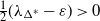 $\frac12({\lambda_{\Delta^{*}} - \varepsilon})>0$
. By Markov’s inequality and using (4.16), we have
$\frac12({\lambda_{\Delta^{*}} - \varepsilon})>0$
. By Markov’s inequality and using (4.16), we have
 \begin{equation*} C(|\widetilde{Y}_n| > {\mathrm{e}}^{-({\lambda_{\Delta^{*}} - \varepsilon})n\hat{\Delta}/2}) \leq \frac{\hat{\mathbb E}\big[\widetilde{Y}^2_n\big]}{{\mathrm{e}}^{-(\lambda_{\Delta^{*}}-\varepsilon)n\hat{\Delta}}} \leq {\mathrm{e}}^{-\varepsilon n\hat{\Delta}}\hat{\mathbb E}\big[\widetilde{Y}^2_0\big]. \end{equation*}
Since $\sum_{n=1}^{\infty}C(|\widetilde{Y}_n| > {\mathrm{e}}^{-(\lambda_{\Delta^{*}} - \varepsilon)n\hat{\Delta}/2}) < \infty$
, owing to the Borel–Cantelli lemma we get
$\sum_{n=1}^{\infty}C(|\widetilde{Y}_n| > {\mathrm{e}}^{-(\lambda_{\Delta^{*}} - \varepsilon)n\hat{\Delta}/2}) < \infty$
, owing to the Borel–Cantelli lemma we get
 \begin{equation*} \limsup_{n \rightarrow \infty} |\widetilde{Y}_n| \leq {\mathrm{e}}^{-(\lambda_{\Delta^{*}} - \varepsilon)n\hat{\Delta}/2} \end{equation*}
quasi-surely. So, there exists $\bar{\Omega} \subset \Omega$
with
$\bar{\Omega} \subset \Omega$
with $C(\bar{\Omega}) = 1$
such that, for all
$C(\bar{\Omega}) = 1$
such that, for all $\omega \in \bar{\Omega}$
and for any
$\omega \in \bar{\Omega}$
and for any $\epsilon>0$
, there exists
$\epsilon>0$
, there exists $n_0(\omega, \epsilon) \in \mathbb{N}$
and
$n_0(\omega, \epsilon) \in \mathbb{N}$
and $|\widetilde{Y}_n(\omega)| \leq {\mathrm{e}}^{-(\lambda_{\Delta^{*}} - \varepsilon)n\hat{\Delta}/2}$
for any
$|\widetilde{Y}_n(\omega)| \leq {\mathrm{e}}^{-(\lambda_{\Delta^{*}} - \varepsilon)n\hat{\Delta}/2}$
for any $n \geq n_0(\omega, \epsilon)$
, and then
$n \geq n_0(\omega, \epsilon)$
, and then
 \begin{equation*} \frac{\log(|\widetilde{Y}_n(\omega)|)}{n\hat{\Delta}} \leq -\bigg(\frac{\lambda_{\Delta^{*}} - \varepsilon}{2}\bigg). \end{equation*}
Ultimately, we have that
 \begin{equation*} \limsup_{n \rightarrow \infty }\frac{\log(|\widetilde{Y}_n|)}{n\hat{\Delta}} \leq -\bigg(\frac{\lambda_{\Delta^{*}} - \varepsilon}{2}\bigg) \quad q.s. \end{equation*}
5. Simulation experiments
In this section we implement the proposed scheme (4.1) for two test problems satisfying conditions (3.2) and (3.3). For this, we need to generate the sample paths of G-Brownian motion. The distribution of G-Brownian motion is defined as $\hat{\mathbb E}[\varphi(B.)]$
for a suitable function
$\hat{\mathbb E}[\varphi(B.)]$
for a suitable function $\varphi$
. As a result, the properties of the G-Brownian motion distribution depend on the selected
$\varphi$
. As a result, the properties of the G-Brownian motion distribution depend on the selected $\varphi$
, and this selection must be uniquely specified whenever we simulate sample paths of the process. In [Reference Yang and Zhao28], the authors focus on the test function
$\varphi$
, and this selection must be uniquely specified whenever we simulate sample paths of the process. In [Reference Yang and Zhao28], the authors focus on the test function $\varphi(x) \, :\!= \, I_{\{x \leq a\}}$
for some
$\varphi(x) \, :\!= \, I_{\{x \leq a\}}$
for some $a \in \mathbb{R}$
, which leads to
$a \in \mathbb{R}$
, which leads to
 \begin{align*} \hat{\mathbb E}[\varphi(B_t)] = \hat{\mathbb E}[I_{\{B_t \leq a\}}] & = \sup\nolimits_{P \in \mathcal{P}} E^P[I_{B_t \leq a}] \\[3pt] & = \sup\nolimits_{P \in \mathcal{P}} P(B_t \leq a) \\[3pt] & = \sup\nolimits_{P \in \mathcal{P}} F^{P}_{B_t}(a).\end{align*}
They initially generate a sample path of the G-Brownian motion at discrete points and subsequently the increments of G-Brownian motion are derived accordingly. Note that all probability measures $P \in \mathcal{P}$
are incorporated in the proposed technique, and that the obtained results correspond to the Heaviside function
$P \in \mathcal{P}$
are incorporated in the proposed technique, and that the obtained results correspond to the Heaviside function $\varphi$
.
$\varphi$
.
The average pathwise error at $T=2$
computed over 100 trajectories for Example 5.1 with the parameters
$T=2$
computed over 100 trajectories for Example 5.1 with the parameters $\underline{\sigma}^2 = 0.5$
and
$\underline{\sigma}^2 = 0.5$
and $\overline{\sigma}^2 = 1$
.
$\overline{\sigma}^2 = 1$
.

The sample paths of the $\theta$
-EM for equation (5.1) are presented with parameters
$\theta$
-EM for equation (5.1) are presented with parameters $\underline{\sigma}^2 = 0.5$
,
$\underline{\sigma}^2 = 0.5$
, $\overline{\sigma}^2 = 1$
, and a step size of
$\overline{\sigma}^2 = 1$
, and a step size of $h = 0.2$
over the interval [0, 2].
$h = 0.2$
over the interval [0, 2].

Example 5.1. The first example, which includes additive noise, is presented as follows:
 \begin{equation} {\mathrm{d}} X_t = -X_t\,{\mathrm{d}} t - \big(X_t + X^3_t\big)\,{\mathrm{d}}\langle B\rangle_t + 0.2\,{\mathrm{d}} B_t, \quad t \geq 0, \ X_0 = 1, \end{equation}
where $(B_t)_{t \geq 0}$
is a G-Brownian motion with
$(B_t)_{t \geq 0}$
is a G-Brownian motion with $\overline{\sigma}^2 = 1$
and
$\overline{\sigma}^2 = 1$
and $\underline{\sigma}^2 = 0.5$
. As we see, the example satiafies the conditions (3.2) for
$\underline{\sigma}^2 = 0.5$
. As we see, the example satiafies the conditions (3.2) for $K_R=1+3R^2$
for any
$K_R=1+3R^2$
for any $R \in \mathbb{R}$
such that
$R \in \mathbb{R}$
such that $|x| \vee |y| \leq R$
, and also the condition (3.3) holds for
$|x| \vee |y| \leq R$
, and also the condition (3.3) holds for $K = 0.04$
. Hence, the equation possesses a unique solution.
$K = 0.04$
. Hence, the equation possesses a unique solution.
Let $\{t_i\}_{i=0}^N$
be a uniform partition of the interval [0, T], where the step size is defined by
$\{t_i\}_{i=0}^N$
be a uniform partition of the interval [0, T], where the step size is defined by $h \, :\!= \, t_{i+1} - t_i$
for each
$h \, :\!= \, t_{i+1} - t_i$
for each $i=0,\ldots,N-1$
. By applying the discretization scheme (4.1) to equation (5.1), we obtain
$i=0,\ldots,N-1$
. By applying the discretization scheme (4.1) to equation (5.1), we obtain
 \begin{equation*} \widetilde{Y}_{i+1} = \frac{1}{1+\theta h}\big((1 - (1-\theta)h)\widetilde{Y}_i - \big(\widetilde{Y}_i + \widetilde{Y}^3_i\big)\Delta\langle B\rangle_i + 0.2\Delta B_i\big), \quad i > 0, \ \theta \in [0,1], \end{equation*}
with $\widetilde{Y}_0 = 0$
. Because an exact closed-form solution is unavailable, we apply the scheme with
$\widetilde{Y}_0 = 0$
. Because an exact closed-form solution is unavailable, we apply the scheme with $\theta = 1$
on a uniform fine discretization grid with a step size of
$\theta = 1$
on a uniform fine discretization grid with a step size of $2^{-10}$
. We calculate
$2^{-10}$
. We calculate
 $$e(t, \omega_j) \, :\!= \, \rvert X(T, \omega_j) - \widetilde{Y}(T, \omega_j)\rvert, \quad j=1,\ldots,100,$$
as an error estimate for the numerical method along each single trajectory. We denote by $\varepsilon$
the average pathwise error calculated over 100 trajectories. Table 1 displays the values of
$\varepsilon$
the average pathwise error calculated over 100 trajectories. Table 1 displays the values of $\varepsilon$
corresponding to
$\varepsilon$
corresponding to $\theta$
in the set
$\theta$
in the set $\{0, 0.5, 1\}$
. As observed, the implicit scheme with
$\{0, 0.5, 1\}$
. As observed, the implicit scheme with $\theta = 1$
outperforms the semi-implicit scheme with
$\theta = 1$
outperforms the semi-implicit scheme with $\theta = \frac{1}{2}$
, which in turn is better than the case with
$\theta = \frac{1}{2}$
, which in turn is better than the case with $\theta =0$
. As expected, reducing the stepsize leads to improved results. Figure 1 illustrates three sample paths of the
$\theta =0$
. As expected, reducing the stepsize leads to improved results. Figure 1 illustrates three sample paths of the $\theta$
-EM equation (5.1).
$\theta$
-EM equation (5.1).
The average pathwise error at $T=3$
computed over 100 trajectories for Example 5.2 with the parameters
$T=3$
computed over 100 trajectories for Example 5.2 with the parameters $\underline{\sigma}^2 = 0.5$
and
$\underline{\sigma}^2 = 0.5$
and $\overline{\sigma}^2 = 1$
.
$\overline{\sigma}^2 = 1$
.

The sample paths of the $\theta$
-EM for equation (5.2) are presented with the parameters
$\theta$
-EM for equation (5.2) are presented with the parameters $\underline{\sigma}^2 = 0.5$
,
$\underline{\sigma}^2 = 0.5$
, $\overline{\sigma}^2 = 1$
, and a step size of
$\overline{\sigma}^2 = 1$
, and a step size of $h = 0.2$
over the interval [0, 2].
$h = 0.2$
over the interval [0, 2].

Example 5.2. The second example, featuring multiplicative noise, is as follows:
 \begin{equation} {\mathrm{d}} X_t = -X_t^5\,{\mathrm{d}} t + {\mathrm{e}}^{-|X_t|/2}\,{\mathrm{d}} B_t, \quad t \geq 0, \ X_0 = 1. \end{equation}
As we can see, the example satisfies the conditions (3.2) and (3.3) with parameters $K_R=1+5R^4$
and
$K_R=1+5R^4$
and $K = 1$
. Similar to Example 5.1, considering the partition
$K = 1$
. Similar to Example 5.1, considering the partition $\{t_i\}_{i=0}^N$
of [0, T] and applying the scheme in (4.1) leads to
$\{t_i\}_{i=0}^N$
of [0, T] and applying the scheme in (4.1) leads to
 \begin{equation*} \widetilde{Y}_{i+1} + \theta h\widetilde{Y}^5_{i+1} = \widetilde{Y}_i - (1-\theta)h\widetilde{Y}^5_{i} + {\mathrm{e}}^{-{|\widetilde{Y}_i|}/{2}}\Delta B_i, \quad i \geq 0, \ \theta \in [0,1]. \end{equation*}
It is clear that $\widetilde{Y}_{t_{i+1}}$
is the root or zero of the real-valued function
$\widetilde{Y}_{t_{i+1}}$
is the root or zero of the real-valued function $f_i$
with
$f_i$
with
 \begin{equation} f_i(x) \, :\!= \, x + \theta hx^5 - c_i, \quad x \in \mathbb{R}, \end{equation}
where $c_i = \widetilde{Y}_i - (1-\theta)h \widetilde{Y}_{i} + {\mathrm{e}}^{-{|\widetilde{Y}_i|}/{2}}\Delta B_i$
. Using the root-finding technique called the Newton–Raphson method, we solve the non-linear equation (5.3) to compute the numerical solutions at the specified points. We need to be mindful of rounding errors when solving non-linear equations numerically. Analogous to Table 1, the smaller step size yields more accurate results, as shown in Table 2. Moreover, Table 2 shows that the semi-implicit method with
$c_i = \widetilde{Y}_i - (1-\theta)h \widetilde{Y}_{i} + {\mathrm{e}}^{-{|\widetilde{Y}_i|}/{2}}\Delta B_i$
. Using the root-finding technique called the Newton–Raphson method, we solve the non-linear equation (5.3) to compute the numerical solutions at the specified points. We need to be mindful of rounding errors when solving non-linear equations numerically. Analogous to Table 1, the smaller step size yields more accurate results, as shown in Table 2. Moreover, Table 2 shows that the semi-implicit method with $\theta=\frac{1}{2}$
and the fully implicit method with
$\theta=\frac{1}{2}$
and the fully implicit method with $\theta=1$
produce more satisfactory results than the explicit method with
$\theta=1$
produce more satisfactory results than the explicit method with $\theta=0$
. However, for step sizes of
$\theta=0$
. However, for step sizes of $2^{-5}$
and
$2^{-5}$
and $2^{-6}$
, the semi-implicit method performs slightly better than the fully implicit one, which could be attributed to the effects of rounding error. Figure 2 illustrates three sample paths of the
$2^{-6}$
, the semi-implicit method performs slightly better than the fully implicit one, which could be attributed to the effects of rounding error. Figure 2 illustrates three sample paths of the $\theta$
-EM equation (5.2).
$\theta$
-EM equation (5.2).
6. Conclusion
To the best of our knowledge, this is the first paper dedicated to numerical solution of the stochastic differential equations driven by G-Brownian motion under locally Lipschitz continuous coefficients. The research outlined designs an implicit continuous Euler–Maruyama scheme to discretize the G-SDE (3.1). Then, the convergence and exponential mean-square stability of the $\theta$
-EM scheme was investigated, which leads to quasi-sure exponential stability as well.
$\theta$
-EM scheme was investigated, which leads to quasi-sure exponential stability as well.
Funding information
This research was in part supported by a grant from IPM (no. 1404600316).
Competing interests
There were no competing interests to declare which arose during the preparation or publication process of this article.

 T=2
T=2 σ_2=0.5
 σ¯2=1
σ¯2=1
 θ
θ σ_2=0.5
 σ¯2=1
σ¯2=1 h=0.2
h=0.2
 T=3
T=3 σ_2=0.5
 σ¯2=1
σ¯2=1
 θ
θ σ_2=0.5
 σ¯2=1
σ¯2=1 h=0.2
h=0.2

