
I. INTRODUCTION
Real-world data often comprise a set of component features, such as images made of a set of pixels and speech comprising a set of frames. These data sets have a hierarchical structure, as illustrated in Fig. 1. We describe data such as images and speech as higher- and lower-level observations. For example, in speech data obtained from a multi-party conversation, higher-level observations correspond to each speaker's utterances, where their variation is caused by the differences in the speakers. Lower-level observations correspond to frame-wise observations comprising each utterance, where their variation is caused by the differences in the contents of speech. To cluster utterances by a speaker, we need to derive a suitable mathematical representation of an utterance for extracting each speaker's characteristics independently of the contents of the their speech [Reference Watanabe, Mochihashi, Hori and Nakamura1].
Hierarchical structure of multi-level data analysis. Segment-wise (higher-level) observations are composed of a set of frame-wise (lower-level) observations. Left figure illustrates the hierarchical structure in speech data composed of frame-wise observations (e.g. Mel-frequency cepstral coefficients).

An effective approach for representing higher-level observations is modeling as stochastic distributions. Thus assume, we that each higher-level observation follows a unique distribution, which represents each speaker's characteristics. Members of exponential families of distributions are employed widely to model higher-level observations due to their usefulness and analytical tractability. However, the underlying assumption of uni-modality for these distributions, is sometimes too restrictive. For example, frame-wise observations, short time fast Fourier transforms of acoustic signals, and filter responses in images are known to follow multi-modal distributions, which cannot be represented by unimodal distributions [Reference Rabiner and Juang2–Reference Spellman, Vemuri and Rao4]. Mixture models are reasonable approximations for representing these multi-modal distributions [Reference Bishop5,Reference McLachlan and Peel6] and various distributions have been used as components of mixture models such as the t-distribution [Reference Andrew, McNicholas and Sudebi7] and von Mises–Fisher distribution [Reference Banerjee, Dhillon, Ghosh and Sra8,Reference Tang, Chu and Huang9]. In particular, Gaussian distributions are used widely as a reasonable approximations for a wide class of probability distributions [Reference Marron and Wand10]. By using a mixture distribution to represent each cluster, the whole speaker space is modeled as a mixture of these mixture distributions. We refer to this as a mixture-of-mixture model. The optimal assignment of higher-level observations to clusters can be obtained by evaluating the posterior probability of assigning each observation to each cluster's mixture distribution. Thus, the clustering problem is reduced to the problem of estimating this mixture-of-mixture model.
The concept of mixture-of-mixture modeling was introduced to analyze multi-modal data sample observations comprising both continuous and categorical variables [Reference Lawrence and Krzanowski11,Reference Willse and Boik12] and data that composed of sets of observations such as data from students nested within schools or patients within hospitals [Reference Calo, Montanari and Viroli13–Reference Vermunt and Magidson15]. However, in these studies, the applications of mixture-of-mixture modeling were limited to simulated or low-dimensional data. In the present study, we focus on applying mixture-of-mixture modeling to speech data, which usually comprises high-dimensional continuous data. In [Reference Calo, Montanari and Viroli13–Reference Vermunt and Magidson15], an expectation–maximization (EM) approach [Reference Dempster, Laird and Rubin16] was used to estimate mixture-of-mixture models by augmenting observations with two-level (higher-level and lower-level) latent variables. However, this maximum-likelihood-based approach often suffers from an overfitting problem when applied to high-dimensional data [Reference Watanabe, Mochihashi, Hori and Nakamura1,Reference Tawara, Ogawa, Watanabe and Kobayashi17]. A Bayesian approach can make the estimation of mixture-of-mixtures models more robust. For example, maximum a posterior (MAP) and variational Bayes (VB)-based methods have been applied to estimate the mixture of Gaussian mixture models (MoGMMs) [Reference Watanabe, Mochihashi, Hori and Nakamura1,Reference Valente, Motlícek and Vijayasenan18,Reference Valente and Wellekens19]. However, the VB-based approach often still suffers from a large bias when the amount of data is limited [Reference Teh, Newman and Welling20]. Moreover, these methods are easily trapped by a local optimum due to the deterministic procedures in the EM-like algorithm.
To solve this problem, we propose a novel MoGMMs estimation method based on the Markov chain Monte Carlo (MCMC) method. In this approach, the optimal parameters for the MoGMMs are obtained stochastically by drawing values iteratively from their posterior distribution. These parameters can be estimated theoretically while avoiding a local optimal solution by evaluating a huge number of samples and combinations of higher-level latent variables (hLVs) Z and lower-level latent variables (lLVs) V from their joint posterior distribution P(Z, V). However, in practical implementations of MCMC, evaluating such a huge number of combinations is infeasible and some approximations are required.
Previously [Reference Watanabe, Mochihashi, Hori and Nakamura1,Reference Tawara, Ogawa, Watanabe and Kobayashi17], we introduced a Gibbs sampling-based MoGMMs estimation approach, which draws the values of lLVs and hLVs alternately by first sampling the lLVs after initializing hLVs Z, i.e., V ~ p(V|Z), and then sampling hLVs by using the fixed lLVs, i.e., Z ~ p(Z|V), sampled in the previous step. This sampling method is easy to implement and highly accurate, and the it actually outperforms the VB-based approach, especially when the data are limited, e.g., when each utterance is short and the spoken utterances are few [Reference Tawara, Ogawa, Watanabe and Kobayashi17]. However, this sampling method, has a severe restriction because the sampling of hLVs is strictly determined by the values of the lLVs obtained in the previous sampling step. This restriction can cause the local optima problem for the hLVs, because the hLVs estimated in each iteration can be highly correlated. To solve this problem, we propose a novel sampling method for the MoGMMs based on nested Gibbs sampling, which samples both the hLVs and lLVs at the same time. This sampling method allow an enormous number of combinations of lLVs and hLVs to be evaluated efficiently, so we can find a more appropriate solution than that obtained by alternating Gibbs sampling for lLVs and hLVs.
The reminder of this paper is organized as follows. In Section II, we formulate a MoGMMs by creating a mixture-of-mixture model where each component of the mixtures is represented by a GMM. In Section III, we explain how to estimate the MoGMMs using fully Bayesian approaches based on VB and MCMC methods. In Section IV, we describe the MCMC-based model estimation method in more detail as well as the proposed nested Gibbs sampling method for MoGMMs estimation. In Section V, we present the results of speaker clustering experiments conducted to demonstrate the effectiveness of the proposed method. In Section VI, we give conclusions and discuss some directions for future research.
II. FORMULATION
In this section, we define the MoGMMs models where each component of the model is represented by a GMM. In addition, we define the generative model for segment-oriented data.
A) MoGMMs
Let ${\bf o}_{ut}\in {\open R}^{D}$
be a D-dimensional observation vector, e.g., mel-frequency cepstral coefficients (MFCCs) at the t-th frame in the u-th segment,
${\bf o}_{ut}\in {\open R}^{D}$
be a D-dimensional observation vector, e.g., mel-frequency cepstral coefficients (MFCCs) at the t-th frame in the u-th segment, ${\bf O}_{u} {\mathop{=}\limits^{\Delta}} \{{\bf o}_{ut}\}_{t=1}^{T_{u}}$
is the u-th segment comprising the T
u
observation vectors, and
${\bf O}_{u} {\mathop{=}\limits^{\Delta}} \{{\bf o}_{ut}\}_{t=1}^{T_{u}}$
is the u-th segment comprising the T
u
observation vectors, and ${\cal O}{\mathop{=}\limits^{\Delta}}\{{\bf O}_{u}\}_{u=1}^{U}$
is a set of U segments. We call this “segment-oriented data.” Here, a MoGMMs is defined as follows:
${\cal O}{\mathop{=}\limits^{\Delta}}\{{\bf O}_{u}\}_{u=1}^{U}$
is a set of U segments. We call this “segment-oriented data.” Here, a MoGMMs is defined as follows:
 $$p({\cal O} \vert {\bf \Theta}) = \prod_{u=1}^{U} \sum_{i=1}^{S} h_{i} p({\bf O}_{u} \vert {\bf \Theta}_{i}),$$
where S denotes the number of clusters; h
i
represents how frequently the i-th cluster's segment appears; and $p({\bf O}_{u} \vert {\bf \Theta}_{i})$
is the likelihood of u-th segment
$p({\bf O}_{u} \vert {\bf \Theta}_{i})$
is the likelihood of u-th segment ${\bf O}_{u}$
being assigned to the i-th cluster. In this case,
${\bf O}_{u}$
being assigned to the i-th cluster. In this case, $p({\bf O}_{u} \vert {\bf \Theta}_{i})$
models the intra-cluster variability for each cluster, which can be represented as:
$p({\bf O}_{u} \vert {\bf \Theta}_{i})$
models the intra-cluster variability for each cluster, which can be represented as:
 $$p({\bf O}_{u} \vert {\bf \Theta}_{i}) = \prod_{t = 1}^{T_{u}} \sum_{j = 1}^{K} w_{ij} {\cal N}({\bf o}_{ut} \vert {\bf \mu}_{ij}, {\bf \Sigma}_{ij}),$$
where ${\cal N}$
denotes the j-th component in the i-th cluster, which is represented by a Gaussian distribution with a mean vector
${\cal N}$
denotes the j-th component in the i-th cluster, which is represented by a Gaussian distribution with a mean vector ${\bf \mu}_{ij}$
and a covariance matrix
${\bf \mu}_{ij}$
and a covariance matrix ${\bf \Sigma}_{ij}$
; w
ij
, the weight of the j-th component; and K is the number of components in each cluster's GMM. Equations (1) and (2) imply that the whole generative model for all segments
${\bf \Sigma}_{ij}$
; w
ij
, the weight of the j-th component; and K is the number of components in each cluster's GMM. Equations (1) and (2) imply that the whole generative model for all segments ${\cal O}$
can be represented by a hierarchically structured MoGMMs where a GMM represents a cluster's characteristics (i.e., intra-cluster variability), and that a mixture of these GMMs can represent the entire cluster space (i.e., inter-cluster variability).
${\cal O}$
can be represented by a hierarchically structured MoGMMs where a GMM represents a cluster's characteristics (i.e., intra-cluster variability), and that a mixture of these GMMs can represent the entire cluster space (i.e., inter-cluster variability).
To represent this hierarchical model, we introduce two types of latent variables: ${\cal Z} = \{z_{u}\}_{u = 1}^{U}$
represents segment-level latent variables (sLVs), each of which identifies a MoGMMs component (i.e., speaker GMM) to which the u-th segment is assigned, and
${\cal Z} = \{z_{u}\}_{u = 1}^{U}$
represents segment-level latent variables (sLVs), each of which identifies a MoGMMs component (i.e., speaker GMM) to which the u-th segment is assigned, and ${\cal V} = \{{\cal V}_{u} = \{v_{ut}\}_{t = 1}^{T_{u}}\}_{u = 1}^{U}$
, represents the frame-level latent variables (fLVs), each of which identifies an intra-cluster GMM component (the cluster distribution to which the u-th segment is assigned), to which the t-th frame-wise observation in the u-th segment is assigned. For instance, the sLVs and fLVs in MoGMMs correspond to the document-level and word-level latent variables in the latent Dirichlet allocation, where discrete data are used [Reference Blei, Ng and Jordan21]. By contrast, we focus on modeling a continuous data space with a MoGMMs in this study.
${\cal V} = \{{\cal V}_{u} = \{v_{ut}\}_{t = 1}^{T_{u}}\}_{u = 1}^{U}$
, represents the frame-level latent variables (fLVs), each of which identifies an intra-cluster GMM component (the cluster distribution to which the u-th segment is assigned), to which the t-th frame-wise observation in the u-th segment is assigned. For instance, the sLVs and fLVs in MoGMMs correspond to the document-level and word-level latent variables in the latent Dirichlet allocation, where discrete data are used [Reference Blei, Ng and Jordan21]. By contrast, we focus on modeling a continuous data space with a MoGMMs in this study.
By introducing these latent variables, we can describe the conditional distributions of the observed segments given the latent variables as followsFootnote 1 :
 $$p({\cal O}\vert {\cal Z},{\cal V}, {\bf \Theta}) = \prod_{u=1}^{U} h_{z_{u}} \prod_{t = 1}^{T_{u}} w_{z_{u}v_{ut}} {\cal N}({\bf o}_{ut} \vert {{\bf \mu}}_{z_{u}v_{ut}}, {\bf \Sigma}_{{z_{u}v_{ut}}}),$$
where ${\bf \Theta} {\mathop{=}\limits^{\Delta}} \{ \{h_{i}\}, \{w_{ij}\}, \{{{\bf \mu}}_{ij}\}, \{{\bf \Sigma}_{ij}\} \}$
denote the weight of the i-th intra-cluster GMM, weight, mean vector, and covariance matrix of the j-th component of the i-th intra-cluster GMM, respectively. Note that we have assumed
${\bf \Theta} {\mathop{=}\limits^{\Delta}} \{ \{h_{i}\}, \{w_{ij}\}, \{{{\bf \mu}}_{ij}\}, \{{\bf \Sigma}_{ij}\} \}$
denote the weight of the i-th intra-cluster GMM, weight, mean vector, and covariance matrix of the j-th component of the i-th intra-cluster GMM, respectively. Note that we have assumed ${\bf \Sigma}_{ij}$
is a diagonal covariance matrix where the (d, d)-th element is represented by σ
ij, d
.
${\bf \Sigma}_{ij}$
is a diagonal covariance matrix where the (d, d)-th element is represented by σ
ij, d
.
We describe the distribution of the latent variables as follows:
 $$P({\cal V} \vert {\cal Z}, {\bf w}) = \prod_{u=1}^{U} \prod_{t=1}^{T_{u}} \prod_{i=1}^{S} \prod_{j=1}^{K} w_{ij}^{\delta(v_{ut},j)\delta(z_{u},i)},$$
 $$P({\cal Z} \vert {\bf h}) = \prod_{u=1}^{U} \prod_{i=1}^{S} h_{i}^{\delta(z_{u},i)},$$
where δ(a, b) denotes Kronecker's delta, which takes a value of one if a=b, and zero otherwise.
B) Generative process and graphical model
Using a Bayesian approach, the conjugate prior distributions of the parameters are often introduced as follows:
 $$p({\bf \Theta} \vert {\bf \Theta}^{0}) = \left\{\matrix{{\bf h} \sim {\cal D}({\bf h}^{0}), \cr {\bf w}_{i} \sim {\cal D}({\bf w}^{0}), \cr \lcub \mu_{ij,d}, \Sigma_{ij,d}\rcub \sim {\cal NG}(\xi^{0}, \eta^{0}, \mu_{j,d}^{0}, \sigma_{j,d}^{0}),}\right.$$
where ${\cal D}({\bf h}^{0})$
and
${\cal D}({\bf h}^{0})$
and ${\cal D}({\bf w}^{0})$
denote Dirichlet distributions with hyper-parameters
${\cal D}({\bf w}^{0})$
denote Dirichlet distributions with hyper-parameters ${\bf h}^{0}$
and
${\bf h}^{0}$
and ${\bf w}^{0}$
, respectively.
${\bf w}^{0}$
, respectively. ${\cal NG}( \xi^{0}, \eta^{0}, \mu_{j,d}^{0}, \sigma_{j,d}^{0} )$
denotes the normal inverse gamma distribution with hyper-parameters ξ0, η0, μ
j,d
0, and σ
j,d
0.
${\cal NG}( \xi^{0}, \eta^{0}, \mu_{j,d}^{0}, \sigma_{j,d}^{0} )$
denotes the normal inverse gamma distribution with hyper-parameters ξ0, η0, μ
j,d
0, and σ
j,d
0.
Based on these likelihoods and prior distributions, the generative process for our model is described as follows:
-
(i) Initialize $\{{\bf h}^{0},{\bf \Theta}^{0}\},$
-
(ii) Draw
${\bf h}$
from
${\cal D}({\bf h}^{0}),$
-
(iii) For each segment-level mixture component (i.e., cluster) i=1, …, S,
-
(a) Draw
${\bf w}_{i}$
from
${\cal D}({\bf w}^{0}),$
-
(b) For each frame-level mixture component (i.e., inner-cluster GMM component) j=1, …, K,
-
(1) Draw
$\{\mu_{i,d},\sigma_{i,d}\}$
from
${\cal NG} (\xi_{j}^{0}, \eta_{j}^{0}, \mu_{j,d}^{0}, \sigma_{j,d}^{0})$
for each dimension d=1, …, D.
-
-
-
(iv) For each segment u=1, …, U,
-
(a) Draw z u from multinomial distribution
${\cal M}({\bf h}),$
-
(b) For each frame
$t=1,\ldots,T_{u}$
,
-
(1) Draw v ut from
${\cal M}({\bf w}_{z_{u}}),$
-
(2) Draw
${\bf o}_{ut}$
from
${\cal N} ({\bf \mu}_{z_{u}v_{ut}}, {\bf \Sigma}_{z_{u}v_{ut}}).$
-
-


Figure 2 shows a graphical representation of this model.
Graphical representation of mixture-of-mixture model. The white square denotes frame-wise observations, and dots denote the hyper-parameters of prior distributions.

III. MODEL INFERENCE BASED ON FULLY BAYESIAN APPROACH
When we use a Bayesian approach for estimating the MoGMMs, the main task is calculating posterior distributions for the latent variables $\{{\cal V}, {\cal Z} \}$
and model parameter
$\{{\cal V}, {\cal Z} \}$
and model parameter ${\bf \Theta}$
given observation
${\bf \Theta}$
given observation ${\cal O}$
:
${\cal O}$
:
 $$p({\cal V}, {\cal Z}, {\bf \Theta} \vert {\cal O}) = {1 \over H_{0}} p({\cal O}, {\cal V}, {\cal Z}, {\bf \Theta}).$$
H 0 is a normalization coefficient, which is defined as follows:
 $$H_{0}{\mathop{=}\limits^{\Delta}} p({\cal O}) = \sum_{{\cal V},{\cal Z}} \int p({\cal O}, {\cal V}, {\cal Z}, {\bf \Theta}) \hbox{d}{\bf \Theta}.$$
Note that the model-based clustering problem is reduced to the problem of estimating the optimal values of the fLVs and sLVs, $\{{\cal V},{\cal Z}\}$
, based on the posterior distribution defined in equation (7). Thus, the posterior probabilities of the latent variables
$\{{\cal V},{\cal Z}\}$
, based on the posterior distribution defined in equation (7). Thus, the posterior probabilities of the latent variables ${\cal V}$
and
${\cal V}$
and ${\cal Z}$
can be calculated as follows:
${\cal Z}$
can be calculated as follows:
 $$\gamma_{v_{ut} = j \vert z_{u} = i; {\bf \Theta}} {\mathop{=}\limits^{\Delta}} p(v_{ut} = j \vert {\bf O}, {\bf \Theta}, z_{u} = i),$$
 $$\gamma_{z_{u} = i; {\bf \Theta}} {\mathop{=}\limits^{\Delta}} p(z_{u} = i \vert {\bf O}, {\bf \Theta}).$$
Sufficient statistics of this model are computed using the aforementioned posterior probabilities as follows:
 $$\left\{\matrix{c_{i} = \sum \nolimits_{u} {\gamma}_{z_{u}=i}, \cr n_{ij} = \sum\nolimits_{u,t} {\gamma}_{v_{ut} = j \vert z_{u} = i} \cdot {\gamma}_{z_{u}=i}, \cr {\bf m}_{ij} = \sum\nolimits_{u,t} {\gamma}_{v_{ut} = j \vert z_{u} = i} \cdot {\gamma}_{z_{u} = i} \cdot {\bf o}_{ut}, \cr r_{ij,d} = \sum \nolimits_{u,t} {\gamma}_{v_{ut} = j \vert z_{u} = i} \cdot {\gamma}_{z_{u} = i} \cdot (o_{ut,d})^{2},} \right.$$
where c i denotes the number of segments assigned to the i-th component of the entire cluster MoGMMs; n ij is the number of frames assigned to the j-th component of the i-th intra-cluster GMM of the MoGMMs; and m ij and r ij are the first and second sufficient statistics, respectively.
However, it is generally infeasible to analytically estimate these posterior distributions, so we must introduce some approximations. In the rest of this section, we discuss how to approximate the posterior distributions using VB- and MCMC-based approaches.
A) Model estimation using a VB-based approach
When the VB-based model estimation method is used, the sLVs, fLVs, and model parameters are obtained deterministically by estimating their variational posterior distributions. To optimize a variational posterior distribution, we attempt to maximize the marginalized likelihood, which is described by equation (8). $ p({\cal V}, {\cal Z}, {\bf \Theta} \vert {\cal O}) = q({\cal V}, {\cal Z}) q({\bf \Theta})$
, where the optimal variational posterior distribution (i.e., the
$ p({\cal V}, {\cal Z}, {\bf \Theta} \vert {\cal O}) = q({\cal V}, {\cal Z}) q({\bf \Theta})$
, where the optimal variational posterior distribution (i.e., the $q({\cal V}, {\cal Z}, {\bf \Theta})$
that maximizes the free energy) can be determined as follows:
$q({\cal V}, {\cal Z}, {\bf \Theta})$
that maximizes the free energy) can be determined as follows:
 $$q({\cal V}, {\cal Z}) \propto \exp \lpar \langle\log p({\cal O}, {\cal V}, {\cal Z}, {\bf \Theta}) \rangle_{q({\bf \Theta})} \rpar ,$$
 $$q({\bf \Theta}) \propto \exp \lpar \langle\log p({\cal O}, {\cal V}, {\cal Z}, {\bf \Theta}) \rangle_{q({\cal V},{\cal Z})} \rpar .$$
where $\langle A \rangle_{B}$
denotes the expectation of A with respect to B. The optimal values of
$\langle A \rangle_{B}$
denotes the expectation of A with respect to B. The optimal values of $q({\cal V}, {\cal Z})$
, and q(Θ) from equations (12) and (13) are obtained according to Algorithm 1, as follows. The posterior probability of an fLV is estimated as follows:
$q({\cal V}, {\cal Z})$
, and q(Θ) from equations (12) and (13) are obtained according to Algorithm 1, as follows. The posterior probability of an fLV is estimated as follows:
 $$\eqalign{\gamma_{v_{ut}} &= j \vert z_{u} = i; \tilde{\bf \Theta}^{\ast} \cr &{\mathop{=}\limits^{\Delta}} \exp \left(\langle \log w_{ij} \rangle_{q(w_{ij})} + {1 \over 2}\sum\nolimits_{d} \langle \log\sigma_{ij,d} \rangle_{q(\sigma_{ij,d})}\right. \cr &\quad - \left. {D \over 2} \log 2\pi \!-\! {1 \over 2} \sum\nolimits_{d} \left\langle {(o_{ut,d}-\mu_{ij,d})^{2} \over \sigma_{ij,d}} \right\rangle_{q(\mu_{ij,d} \vert \sigma_{ij,d})} \right).}$$
We can determine the posterior distribution of an fLV by normalizing (14) as follows:
 $$q(v_{ut} = j \vert z_{u} = i) = {\gamma_{v_{ut}=j \vert z_{u}=i;\tilde{{\bf \Theta}}}^{\ast} \over \sum\nolimits_{j}\gamma_{v_{ut} = j \vert z_{u}=i;\tilde{\bf \Theta}}^{\ast}}.$$
In the same manner, we can compute an sLV $\gamma_{z_{u}=i;\tilde{{\bf \Theta}}}$
from the posterior probability
$\gamma_{z_{u}=i;\tilde{{\bf \Theta}}}$
from the posterior probability $\gamma_{z_{u}=i;\tilde{{\bf \Theta}}}^{\ast}$
as follows:
$\gamma_{z_{u}=i;\tilde{{\bf \Theta}}}^{\ast}$
as follows:
 $$\gamma_{z_{u}=i;\tilde{\bf \Theta}}^{\ast} {\mathop{=}\limits^{\Delta}} \exp \left(\!\langle \log h_{i} \rangle_{q(h_{i})} + \sum_{t}\log \sum_{j}\gamma_{v_{ut}=j \vert z_{u}=i;\tilde{{\bf \Theta}}}^{\ast} \!\right),$$
 $$q(z_{u} = i) = {\gamma_{z_{u} = i;\tilde{\bf \Theta}}^{\ast} \over \sum\nolimits_{i} \gamma_{z_{u} = i; \tilde{\bf \Theta}}^{\ast}}.$$
The expected values of the parameters described in (14)–(16) are computed as follows:
 $$\langle \log h_{i} \rangle_{q(h_{i})} = \psi(\tilde{h}_{i}) - \psi \left(\sum\nolimits_{i} \tilde{h}_{i}\right),$$
 $$\langle \log w_{ij} \rangle_{q(w_{ij})} = \psi (\tilde{w}_{ij}) - \psi \left(\sum\nolimits_{j}\tilde{w}_{ij}\right),$$
 $$\langle \log \sigma_{ij,d} \rangle_{q(\sigma_{ij,d})} = \psi (\tilde{\eta}_{ij}) - \log \tilde{\sigma}_{ij,d},$$
 $$\left\langle {(o_{ut,d} - \mu_{ij,d})^{2} \over \sigma_{ij,d}} \right\rangle_{q(\mu_{ij,d} \vert \sigma_{ij,d})} = {\tilde{\eta}_{ij} (o_{ut,d} \!-\! \tilde{\mu}_{ij,d})^{2} + \tilde{\xi}_{ij} \over \tilde{\sigma}_{ij,d}},$$
where ψ(·) denotes the digamma function and $\tilde{\bf \Theta} = \{ \tilde{h}_{i}, \tilde{w}_{ij}, \tilde{\xi}_{ij}, \tilde{\eta}_{ij}, \tilde{\bf \mu}_{ij} \}$
are the hyper-parameters of the posterior distributions for
$\tilde{\bf \Theta} = \{ \tilde{h}_{i}, \tilde{w}_{ij}, \tilde{\xi}_{ij}, \tilde{\eta}_{ij}, \tilde{\bf \mu}_{ij} \}$
are the hyper-parameters of the posterior distributions for $\tilde{\bf \Theta}$
, which are computed as follows:
$\tilde{\bf \Theta}$
, which are computed as follows:
 $$\tilde{{\bf \Theta}} = \left\{\matrix{\tilde{h}_{i} = h^{0} + c_{i}, \cr \tilde{w}_{ij} = w_{j}^{0} + n_{ij}, \cr \tilde{\xi}_{ij} = \xi^{0} + n_{ij}, \cr \tilde{\eta}_{ij} = \eta^{0} + n_{ij}, \cr \tilde{{\bf \mu}}_{ij} = \tilde{\xi}_{ij}^{-1} (\xi^{0}{{\bf \mu}}_{j}^{0} + {\bf m}_{ij}), \cr \tilde{\sigma}_{ij,d} = \sigma_{j,d}^{0} + r_{ij,d} + \xi^{0}(\mu_{j,d}^{0})^{2} - \tilde{\xi}_{ij}(\tilde{\mu}_{ij,d})^{2}.} \right.$$
Algorithm 1 shows the VB-based model estimation algorithm. The fLVs and sLVs that maximize (equations (15) and (17)) are the MAP values of their posterior distributions, where we assume that these MAP values are the optimal clustering results.
Model estimation algorithm using the VB method.

This VB-based procedure monotonically increases the free energy, as described in equation (8) under the variational posterior distribution $q({\cal V},{\cal Z},{\bf \Theta})$
, but this approach suffers from two problems, which are caused by the difference between true and variational posterior distributions, as well as the biased values. The first problem is that the true posterior distributions of fLVs, sLVs, and the model parameters in MoGMMs cannot be factorized (i.e.,
$q({\cal V},{\cal Z},{\bf \Theta})$
, but this approach suffers from two problems, which are caused by the difference between true and variational posterior distributions, as well as the biased values. The first problem is that the true posterior distributions of fLVs, sLVs, and the model parameters in MoGMMs cannot be factorized (i.e., $p({\bf \Theta}, {\cal V}, {\cal Z} \vert {\cal O}) \neq p({\cal V} \vert {\cal Z}, {\cal O}) p({\cal Z} \vert {\cal O})p({\bf \Theta} \vert {\cal O})$
), although the variational posterior distributions assume that they can. The second problem is that the posterior probability obtained is generally biased because the calculated statistics are strongly biased by the size of each segment. These problems are especially severe when the number of segments is limited. To solve these problems, we need to estimate the marginalized posterior distributions, into which model parameter
$p({\bf \Theta}, {\cal V}, {\cal Z} \vert {\cal O}) \neq p({\cal V} \vert {\cal Z}, {\cal O}) p({\cal Z} \vert {\cal O})p({\bf \Theta} \vert {\cal O})$
), although the variational posterior distributions assume that they can. The second problem is that the posterior probability obtained is generally biased because the calculated statistics are strongly biased by the size of each segment. These problems are especially severe when the number of segments is limited. To solve these problems, we need to estimate the marginalized posterior distributions, into which model parameter ${\bf \Theta}$
and fLVs
${\bf \Theta}$
and fLVs ${\cal V}$
are collapsedFootnote
2
. This is obtained by marginalizing equation (7) with respect to these parameters as follows:
${\cal V}$
are collapsedFootnote
2
. This is obtained by marginalizing equation (7) with respect to these parameters as follows:
 $$P({\cal V}, {\cal Z} \vert {\cal O}) = {1 \over H_0} \int p({\cal V}, {\cal Z}, {\bf \Theta}, {\cal O}). \hbox{d}{\bf \Theta}.$$
We can then estimate the posterior distribution of the latent variables directly and obtain an unbiased estimation.
Collapsed VB methods for estimating the marginalized posterior distribution have been proposed in several studies [Reference Sung, Ghahramani and Bang22,Reference Teh, Newman and Welling23], but these approaches are generally infeasible for our hierarchical model because we cannot apply the approximation of convexity to a hierarchical structure. Therefore, we introduce the MCMC method to estimate the marginalized posterior distribution from equation (23).
B) Model estimation based on the MCMC approach
Using an MCMC-based approach, we obtain samples of latent variables directly from their posterior distributions. We can derive the marginalized distribution with respect to the model parameters described in equation (23) because we do not need to evaluate the normalization term equation (8) when employing an MCMC approach.
1) Marginalized likelihood for complete data
First, we derive the logarithmic marginalized likelihood for the complete data, $\log p({\cal O}, {\cal V}, {\cal Z})$
. In the case of complete data, we can utilize all the alignments of observations
$\log p({\cal O}, {\cal V}, {\cal Z})$
. In the case of complete data, we can utilize all the alignments of observations ${\bf o}_{ut}$
to a specific Gaussian component distribution because all of the latent variables,
${\bf o}_{ut}$
to a specific Gaussian component distribution because all of the latent variables, $\{{\cal V},{\cal Z}\}$
, are treated as observations. Then, the posterior distributions for each of the latent variables,
$\{{\cal V},{\cal Z}\}$
, are treated as observations. Then, the posterior distributions for each of the latent variables, $P(z_{u} = i \vert \cdot)$
and
$P(z_{u} = i \vert \cdot)$
and $P(v_{ut} = j \vert \cdot)$
for all i, j, u, and t, return 0 or 1 based on the assigned information. Thus,
$P(v_{ut} = j \vert \cdot)$
for all i, j, u, and t, return 0 or 1 based on the assigned information. Thus, $\gamma_{v_{ut}=j \vert z_{u}=i}$
and
$\gamma_{v_{ut}=j \vert z_{u}=i}$
and $\gamma_{z_{u}=i}$
described by equations (9) and (10) are zero-or-one values depending on the assignment of the data. Then, the sufficient statistics of this model, then, can be represented as follows:
$\gamma_{z_{u}=i}$
described by equations (9) and (10) are zero-or-one values depending on the assignment of the data. Then, the sufficient statistics of this model, then, can be represented as follows:
 $$\left\{\matrix{c_{i} = \sum \nolimits_{u} \delta(z_{u},i), \cr n_{ij} = \sum \nolimits_{u,t} \delta(z_{u},i) \cdot \delta(v_{ut},j), \cr {\bf m}_{ij} = \sum \nolimits_{u,t} \delta(z_{u},i) \cdot \delta(v_{ut},j) \cdot {\bf o}_{ut}, \cr r_{ij,d} = \sum \nolimits_{u,t} \delta(z_{u},i) \cdot \delta(v_{ut},j) \cdot (o_{ut,d})^{2},}\right.$$
We can analytically derive the logarithmic marginalized likelihood for the complete data by substituting equations (3)–(5) into the following integration equation:
 $$\eqalign{&\log p({\cal V}, {\cal Z}, {\cal O}) \cr & \quad = \log \int p({\cal V}, {\cal Z},{\cal O} \vert {\bf \Theta}) p({\bf \Theta}) \hbox{d}{\bf \Theta} \cr & \quad= \log { \Gamma(h^{0}) \prod_{i} \Gamma(\tilde{h}_{i}) \over \Gamma (h^{0})^{S} \Gamma \left(\sum_{i} \tilde{h}_{i}\right)} + \log \prod_{i} {\Gamma \left(\sum_{j} w_{j}^{0} \right) \prod_{j} \Gamma (\tilde{w}_{ij}) \over \prod_{j} \Gamma (w_{j}^{0}) \Gamma \left(\sum_{j} \tilde{w}_{ij}\right)} \cr & \qquad + \beta \log \prod_{i,j} (2\pi)^{-{n_{ij}D \over 2}} {(\xi^{0})^{D \over2} \left(\Gamma \left({\eta_{j}^{0} \over 2} \right) \right)^{-D} \left(\prod_{d}\sigma_{j,dd}^{0} \right)^{\eta_{j}^{0} \over 2} \over (\tilde{\xi}_{ij})^{D \over 2} \left(\Gamma \left({\tilde{\eta}_{ij} \over 2} \right)\right)^{-D} \left(\prod_{d}\tilde{\sigma}_{ij,dd}\right)^{\tilde{\eta}_{ij} \over2}},}$$
where $\tilde{\bf \Theta}_{ij}{\mathop{=}\limits^{\Delta}} \{ \tilde{h}_{i}, \tilde{w}_{ij}, \tilde{\xi}_{ij}, \tilde{\eta}_{ij}, \tilde{\mu}_{ij,d}, \tilde{\sigma}_{ij,d} \} $
denotes the hyper-parameter of the marginalized likelihood defined in equation (22).
$\tilde{\bf \Theta}_{ij}{\mathop{=}\limits^{\Delta}} \{ \tilde{h}_{i}, \tilde{w}_{ij}, \tilde{\xi}_{ij}, \tilde{\eta}_{ij}, \tilde{\mu}_{ij,d}, \tilde{\sigma}_{ij,d} \} $
denotes the hyper-parameter of the marginalized likelihood defined in equation (22).
To construct the MCMC sampler, we define the following logarithmic likelihood function for the complete data using simulated annealing (SA) [Reference Kirkpatrick, Gelatt and Vecchi24]:
 $$\eqalign{H_{p}(\beta) &{\mathop{=}\limits^{\Delta}} \log p_{\beta}({\cal V},{\cal Z},{\cal O}) \cr &= \log p({\cal O}\vert {\cal V}, {\cal Z}) + {1 \over \beta} \log P({\cal V}, {\cal Z}),}$$
where β is an inverse temperature defined for SA, which controls the speed of convergence. We can now derive the posterior distribution as follows:
 $$\eqalign{P({\cal V},{\cal Z} \vert {\cal O}) &= {1 \over H_{p}(\beta)} p({\cal V}, {\cal Z}) p({\cal O} \vert {\cal V}, {\cal Z})^{\beta} \cr &= {1 \over H_{p}(\beta)} \exp \lcub -\beta H({\bf \Psi})\rcub ,}$$
where H
p
(β) is a normalization term introduced to normalize $\{{\cal V},{\cal Z}\}$
under the temperature β. The goal of the MCMC approach is to obtain samples from equation (27). In the next section, we discuss how to design the sampler in order to obtain samples from this posterior distribution.
$\{{\cal V},{\cal Z}\}$
under the temperature β. The goal of the MCMC approach is to obtain samples from equation (27). In the next section, we discuss how to design the sampler in order to obtain samples from this posterior distribution.
IV. IMPLEMENTATION OF MCMC-BASED MODEL ESTIMATION
We introduce a collapsed Gibbs sampler [Reference Liu25] to obtain samples of sLVs and fLVs from their posterior distributions. Previously, we introduced a Gibbs assumption that alternates the sampling of fLVs with some initializations of sLVs, before sampling the sLVs using the fixed fLVs sampled in the previous step [Reference Watanabe, Mochihashi, Hori and Nakamura1,Reference Tawara, Ogawa, Watanabe and Kobayashi17]. The drawback of this approach is that the sampling of sLVs is determined strictly by the values of the fLVs obtained in the previous sampling step and the sLVs estimated in each iteration can be highly correlated. To solve this problem, we propose a novel sampling method that samples both sLVs and fLVs at the same time. This sampling method allows an enormous number of combinations of fLVs and sLVs to be evaluated efficiently, so we can find a more appropriate solution than that obtained when alternating Gibbs sampling for fLVs and sLVs. We refer to this novel sampling technique as nested Gibbs sampling. This section describes its formulation and implementation.
A) Nested Gibbs sampling for MoGMMs
For Gibbs sampling, we draw the value of each variable iteratively from its posterior distributions and conditioning it with the sampled values of the other variables. This posterior distribution is called the “proposal distribution.” In the case of MoGMMs, the proposal distribution is the joint posterior distribution of the sLV and fLVs related to the u-th segment of $\{{\cal V}_{u}, z_{u}\}$
, which is conditioned on the sampled value of the latent variables related to the other segments
$\{{\cal V}_{u}, z_{u}\}$
, which is conditioned on the sampled value of the latent variables related to the other segments $\{{\cal V}_{\backslash u}^{\ast}, {\cal Z}_{\backslash u}^{\ast} \}$
. Therefore, the proposal distribution of MoGMMs is described as follows:
$\{{\cal V}_{\backslash u}^{\ast}, {\cal Z}_{\backslash u}^{\ast} \}$
. Therefore, the proposal distribution of MoGMMs is described as follows:
 $$P \lpar {\cal V}_{u}, z_{u} \vert \lcub {\cal V}_{\backslash u}^{\ast}, {\cal Z}_{\backslash u}^{\ast} \rcub , {\cal O} \rpar = {p\lpar {\cal V}_{u}, z_{u}, \lcub {\cal V}_{\backslash u}^{\ast}, {\cal Z}_{\backslash u}^{\ast} \rcub , {\cal O} \rpar \over p\lpar \lcub {\cal V}_{\backslash u}^{\ast}, {\cal Z}_{\backslash u}^{\ast}\rcub , {\cal O} \rpar },$$
where ${\cal V}_{\backslash u}^{\ast} = \{v_{u^{\prime} t}^{\ast} \vert \forall u^{\prime} \neq u,\forall t\}$
and
${\cal V}_{\backslash u}^{\ast} = \{v_{u^{\prime} t}^{\ast} \vert \forall u^{\prime} \neq u,\forall t\}$
and ${\cal Z}_{\backslash u}^{\ast} = \{z_{u^{\prime}}^{\ast} \vert \forall u^{\prime} \neq u\}$
denote the sets of samples for fLVs and sLVs, respectively, except for those related to the u-th segment. After some iterative sampling using equation (28), the samples obtained are approximately distributed according to their true posterior distributions. Direct sampling from a proposal distribution equation (28) is theoretically feasible because equation (28) takes the form of a multinomial distribution. However, it is impractical to evaluate an enormous number of possible combinations of solutions. We notice that it is enough to estimate the value of sLVs in order to estimate the optimal assignment of utterances to speaker clusters. Therefore, we try to marginalize out fLVs in equation (28) to make the computation simple. We propose an MCMC-based approach, which samples the value of z
u
directly from the following marginalized posterior instead of equation (28):
${\cal Z}_{\backslash u}^{\ast} = \{z_{u^{\prime}}^{\ast} \vert \forall u^{\prime} \neq u\}$
denote the sets of samples for fLVs and sLVs, respectively, except for those related to the u-th segment. After some iterative sampling using equation (28), the samples obtained are approximately distributed according to their true posterior distributions. Direct sampling from a proposal distribution equation (28) is theoretically feasible because equation (28) takes the form of a multinomial distribution. However, it is impractical to evaluate an enormous number of possible combinations of solutions. We notice that it is enough to estimate the value of sLVs in order to estimate the optimal assignment of utterances to speaker clusters. Therefore, we try to marginalize out fLVs in equation (28) to make the computation simple. We propose an MCMC-based approach, which samples the value of z
u
directly from the following marginalized posterior instead of equation (28):
 $$\eqalign{p\lpar z_{u} \vert \lcub {\cal V}_{\backslash u}^{\ast}, {\cal Z}_{\backslash u}^{\ast} \rcub , {\cal O} \rpar & = \int p \lpar z_{u} \vert {\cal V}_{u}^{\ast}, \lcub {\cal V}^{\ast}_{\backslash u},{\cal Z}^{\ast}_{\backslash u} \rcub , {\cal O} \rpar \cr & \quad \times p\lpar {\cal V}_{u}^{\ast} \vert \lcub {\cal V}_{\backslash u}^{\ast}, {\cal Z}_{\backslash u}^{\ast} \rcub , {\cal O} \rpar \hbox{d} {\cal V}_{u}.}$$
However, this integration is also infeasible because each v
ut
in ${\cal V}_{u}$
takes one of the number of K values (i.e., the number of GMM components) and their combination are exponentially large. Therefore, we introduce an approximated approach, which uses the sampled value of
${\cal V}_{u}$
takes one of the number of K values (i.e., the number of GMM components) and their combination are exponentially large. Therefore, we introduce an approximated approach, which uses the sampled value of ${\cal V}_{u}^{\ast \ast }$
obtained from its true posterior
${\cal V}_{u}^{\ast \ast }$
obtained from its true posterior $p({\cal V}^{\ast}_{u} \vert \{{\cal V}^{\ast}_{\backslash u}, {\cal Z}_{\backslash u}^{\ast}\}, {\cal O})$
. Then,
$p({\cal V}^{\ast}_{u} \vert \{{\cal V}^{\ast}_{\backslash u}, {\cal Z}_{\backslash u}^{\ast}\}, {\cal O})$
. Then, ${\cal V}_{u}^{\ast}$
is marginalized out from equation (28) using the sampled value
${\cal V}_{u}^{\ast}$
is marginalized out from equation (28) using the sampled value ${\cal V}_{u}^{\ast \ast }$
by the following approximation:
${\cal V}_{u}^{\ast \ast }$
by the following approximation:
 $$p \lpar z_{u} \vert \lcub {\cal V}_{\backslash u}^{\ast}, {\cal Z}_{\backslash u}^{\ast} \rcub , {\cal O} \rpar \simeq \sum_{{\cal V}_{u}^{\ast \ast}} P\lpar z_{u} \vert {\cal V}_{u}^{\ast \ast}, \lcub {\cal V}_{\backslash u}^{\ast}, {\cal Z}_{\backslash u}^{\ast} \rcub , {\cal O}\rpar .$$
We can easily sample the value of z
u
from equation (30) because this is a multinomial distribution over z
u
that takes the one of the C (i.e., number of clusters) values. With this approach, the Gibbs sampling chain for z
u
is followed by another Gibbs sampling chain in which we sample the values of ${{\cal V}_{u}}$
from its posterior distribution, conditioned on any potential value of z
u
. We refer to this Gibbs sampler for
${{\cal V}_{u}}$
from its posterior distribution, conditioned on any potential value of z
u
. We refer to this Gibbs sampler for ${\cal V}_{u}$
as a sub-Gibbs sampler and we refer to the obtained samples as
${\cal V}_{u}$
as a sub-Gibbs sampler and we refer to the obtained samples as ${\cal V}_{u \vert z_{u}=i}^{\ast \ast} = \{v_{ut \vert z_{u=i}}^{\ast \ast}\}_{t = 1}^{T_{u}}$
. In the sub-Gibbs sampler, each value of
${\cal V}_{u \vert z_{u}=i}^{\ast \ast} = \{v_{ut \vert z_{u=i}}^{\ast \ast}\}_{t = 1}^{T_{u}}$
. In the sub-Gibbs sampler, each value of $v_{ut \vert z_{u}=i}^{\ast \ast}$
is sampled for all i as follows:
$v_{ut \vert z_{u}=i}^{\ast \ast}$
is sampled for all i as follows:
 $$v_{ut \vert z_{u} = i}^{\ast \ast} \sim P\lpar v_{ut} \vert \lcub {\cal V}_{\backslash u}^{\ast}, {\cal Z}_{\backslash u}^{\ast} \rcub , {\cal V}_{u\backslash t}^{\ast \ast}, z_{u} = i, {\cal O}\rpar ,$$
where ${\cal V}_{u\backslash t \vert z_{u}=i}^{\ast \ast} = \{ v_{ut^{\prime} \vert z_{u} = i}^{\ast \ast} \vert \forall t^{\prime} \neq t\}$
denotes the samples of fLVs obtained from the sub-Gibbs sampler that are related to all of the frames, except to the t-th frame in the u-th segment. After several iterations of equation (31) for all t in the u-th segment, we obtain
${\cal V}_{u\backslash t \vert z_{u}=i}^{\ast \ast} = \{ v_{ut^{\prime} \vert z_{u} = i}^{\ast \ast} \vert \forall t^{\prime} \neq t\}$
denotes the samples of fLVs obtained from the sub-Gibbs sampler that are related to all of the frames, except to the t-th frame in the u-th segment. After several iterations of equation (31) for all t in the u-th segment, we obtain $N^{Gibbs}$
samples. We then draw a sample of sLV for the u-th segment from its posterior distribution conditioned on the samples
$N^{Gibbs}$
samples. We then draw a sample of sLV for the u-th segment from its posterior distribution conditioned on the samples $\{{{\cal V}_{u\vert z_{u} = i}^{\ast \ast}}^{(n)}\}_{n=1}^{N^{Gibbs}}$
. By aggregating the value of
$\{{{\cal V}_{u\vert z_{u} = i}^{\ast \ast}}^{(n)}\}_{n=1}^{N^{Gibbs}}$
. By aggregating the value of $\{{{\cal V}_{u\vert z_{u}=i}^{\ast \ast}}^{(n)} \}_{n = 1}^{N^{Gibbs}}$
over all possible values of i, the Gibbs sampler for z
u
is defined as follows:
$\{{{\cal V}_{u\vert z_{u}=i}^{\ast \ast}}^{(n)} \}_{n = 1}^{N^{Gibbs}}$
over all possible values of i, the Gibbs sampler for z
u
is defined as follows:
 $$\eqalign{z_{u} &\sim P(z_{u} \vert \lcub {\cal V}_{\backslash u}^{\ast}, {\cal Z}_{\backslash u}^{\ast} \rcub , {\cal O}) \cr &= \sum_{\forall {\cal V}_{u}} P \lpar {\cal V}_{u}, z_{u} \vert \lcub {\cal V}_{\backslash u}^{\ast}, {\cal Z}_{\backslash u}^{\ast} \rcub , {\cal O} \rpar \cr &= \sum_{\forall{\cal V}_{u}} P \lpar z_{u} \vert \lcub {\cal V}_{\backslash u}^{\ast}, {\cal Z}_{\backslash u}^{\ast} \rcub , {\cal V}_{u}, {\cal O} \rpar P \lpar {\cal V}_{u} \vert \lcub {\cal V}_{\backslash u}^{\ast}, {\cal Z}_{\backslash u}^{\ast} \rcub , {\cal O} \rpar .}$$
Model estimation algorithm based on the proposed nested Gibbs sampling method.

By aggregating $N^{Gibbs}$
samples of
$N^{Gibbs}$
samples of ${\cal V}_{u}$
from
${\cal V}_{u}$
from $p({\cal V}_{u} \vert z_{u} = i, \{{\cal V}_{\backslash u}^{\ast}, {\cal Z}_{\backslash u}^{\ast}\},{\cal O})$
for all possible values of i and then plugging them into
$p({\cal V}_{u} \vert z_{u} = i, \{{\cal V}_{\backslash u}^{\ast}, {\cal Z}_{\backslash u}^{\ast}\},{\cal O})$
for all possible values of i and then plugging them into $p(z_{u} \vert V_{u}, O)$
, we obtain the following Monte Carlo integration:
$p(z_{u} \vert V_{u}, O)$
, we obtain the following Monte Carlo integration:
 $$\eqalign{&\sum_{\forall{\cal V}_{u}} P\lpar z_{u} \vert \lcub {\cal V}_{\backslash u}^{\ast}, {\cal Z}_{\backslash u}^{\ast} \rcub , {\cal V}_{u}, {\cal O} \rpar P \lpar {\cal V}_{u} \vert \lcub {\cal V}_{\backslash u}^{\ast}, {\cal Z}_{\backslash u}^{\ast} \rcub , {\cal O} \rpar \cr & \quad \simeq {1 \over N^{Gibbs}} \sum_{n = 1}^{N^{Gibbs}} P\lpar z_{u} \vert {{\cal V}_{u}^{\ast \ast}}^{(n)}, \lcub {\cal V}_{\backslash u}^{\ast}, {\cal Z}_{\backslash u}^{\ast}\rcub , {\cal O}\rpar .}$$
We refer to these procedures as nested Gibbs sampling, because we sample z
u
from equation (33) using the value of ${\cal V}_{u}^{\ast \ast (n)}$
which can be obtained from the sub-Gibbs sampler defined by equation (31) in a nested manner. A large number of samples,
${\cal V}_{u}^{\ast \ast (n)}$
which can be obtained from the sub-Gibbs sampler defined by equation (31) in a nested manner. A large number of samples, $N^{Gibbs}$
, may be required to accurately represent of the marginal value for equation (33). To evaluate the effect of the number of samples on the overall sampling procedure, we applied the proposed nested Gibbs sampler to practical speech data. Figure 3 shows the logarithmic marginalized likelihoods (LMLs) obtained using the proposed nested Gibbs sampling method with different sampling sizes. The eight lines in each figure correspond to the results of eight trials with different random seeds. This figure shows that high accuracy may be achieved with a small number of samples, and that even one sample may be adequate to approximate the marginal value in equation (33). Algorithm 2 shows the algorithm of the nested Gibbs sampler for MoGMMs. The formulations of equations (31) and (33) are described in the Appendix.
$N^{Gibbs}$
, may be required to accurately represent of the marginal value for equation (33). To evaluate the effect of the number of samples on the overall sampling procedure, we applied the proposed nested Gibbs sampler to practical speech data. Figure 3 shows the logarithmic marginalized likelihoods (LMLs) obtained using the proposed nested Gibbs sampling method with different sampling sizes. The eight lines in each figure correspond to the results of eight trials with different random seeds. This figure shows that high accuracy may be achieved with a small number of samples, and that even one sample may be adequate to approximate the marginal value in equation (33). Algorithm 2 shows the algorithm of the nested Gibbs sampler for MoGMMs. The formulations of equations (31) and (33) are described in the Appendix.
LML obtained using proposed nested Gibbs sampler, applied to A1+station noise. Refer to Table 1 for the details of test set A1. Each figure shows results with a different sampling size N samp . Eight lines correspond to results of eight trials using different random seeds. (a) N Gibbs =1 & (b) N Gibbs =5

B) Computation of the marginalized likelihood
For the Gibbs sampler described in A, we can approximate the joint likelihood equation (26) using the sampled latent variables $\{{\cal V}^{\ast}_{u},{\cal Z}^{\ast}_{u}\}_{u=1}^{U}$
.
$\{{\cal V}^{\ast}_{u},{\cal Z}^{\ast}_{u}\}_{u=1}^{U}$
.
Figure 4 is a scatter diagram showing the marginalized likelihood and K values (which are used widely for the measurement of the clustering) calculated from the results obtained when the proposed nested Gibbs sampler was applied to B1 and B1 with four types of noise. The values of K are explained in the Experiment section. The differences in the plots indicate the distinct speakers. This figure shows that the value of K is strongly correlated with the marginalized likelihood. Therefore, we can use the marginalized likelihood as a measure of the appropriateness of the models.
LML as a function of K value. Each plot shows the results obtained by applying the proposed n-Gibbs sampler to five different datasets (id:000, 001, …, 004). Refer to Table 1 for the details of test set B1. (a) B1 (clean) & (b) B1+crowd (c) B1+street & (d) B2+party (e) B2+station

V. SPEAKER CLUSTERING EXPERIMENTS
We investigated the effectiveness of our model optimization methods at speaker clustering using the TIMIT [Reference Garofolo, Lamel, Fisher, Fiscus, Pallett and Dahlgren26] and CSJ [Reference Kawahara, Nanjo and Furui27] databases. We compared the following four model estimation methods:
-
• n-Gibbs: MCMC-based model estimation using the proposed nested Gibbs sampling method.
-
• Gibbs: MCMC-based model estimation using conventional Gibbs sampling where the fLVs and sLVs are sampled alternately [Reference Watanabe, Mochihashi, Hori and Nakamura1,Reference Tawara, Ogawa, Watanabe and Kobayashi17].
-
• VB: VB-based model estimation [Reference Valente and Wellekens19].
-
• HAC-GMM: hierarchical agglomerative clustering method. A GMM is estimated for each utterance in a maximum-likelihood manner. The similarity between utterances is defined as the cross likelihood ratio between corresponding GMMs. The pair of utterances with the greatest similarity is merged iteratively until the correct number of speakers is obtained [Reference Reynolds, Quatieri and Dunn3].
A) Experimental setup
1) Datasets
All of the experiments were conducted using 11 evaluation sets obtained from TIMIT and CSJ. Table 1 lists the number of speakers and utterances in the evaluation sets used. T1 and T2 were constructed using TIMIT. T1 corresponds to the core test set of TIMIT, which includes 192 utterances from 24 speakers. T2 is the complete test set, which includes 1152 utterances from 144 speakers. In this case, there were no overlaps between T1 and T2. The remaining nine evaluation sets were constructed using CSJ as follows: all lecture speech in CSJ was divided into utterance units based on the silence segments in their transcriptions, five speakers were then randomly selected, and five, 10, and 20 of their utterances were chosen for A1, A2, and A3, respectively. In the same manner, we randomly selected 10 and 15 different speakers and five, 10, and 20 of their utterances were used for B1 to B3 and C1 to C3, respectively. We evaluated five combinations of different speakers for each dataset. The resulting clustering performance for each dataset was the average of these five combinations.
Details of test set.

The speech data from TIMIT and CSJ are not corrupted by noise. In additional experiments, we used noisy speech data, which we created by overlapping each utterance with four types of non-stationary noise (crowd, street, party, and station) selected from the noise database of the Japan Electronic Industry Development Association [Reference Shuichi28]. These noises were overlapped with each utterance at a signal-to-noise ratio of about 10 dB. Speech data were sampled at 16 kHz and quantized into 16-bit data. We used 26-dimensional acoustic feature parameters, which comprised 12-dimensional MFCCs with log energy and their Δ parameters. The frame length and frame shift were 25 and 10 ms, respectively.
2) Measurement
We employed the average cluster purity (ACP), average speaker purity (ASP), and their geometric means (K value) as the speaker clustering evaluation criteria [Reference Solomonoff, Mielke, Schmidt and Gish29]. In this experiment, the correct speaker label was manually annotated for each utterance. Let S T be the correct number of speakers; S is the estimated number of speakers; n ij is the estimated number of utterances assigned to speaker cluster i in all utterances by speaker j; n j is the estimated number of utterances of speaker j; n i is the estimated number of utterances assigned to speaker cluster i; and U is the number of all utterances. The cluster purity p i and speaker purity q j were then calculated as follows.
 $$p_{i} = \sum_{j = 0}^{S_{T}} {n_{ij}^{2} \over n_{i}^{2}}, \quad q_{j} = \sum_{i = 0}^{S} {n_{ij}^{2} \over n_{j}^{2}}.$$
The cluster purity is the ratio of utterances derived from the same speaker relative to the utterances assigned to each cluster. The speaker purity is the ratio of utterances assigned to the same cluster relative to the utterances spoken by each speaker. Thus, ACP and ASP are calculated as follows.
 $$V_{\rm ACP} = {1 \over U} \sum_{i = 0}^{S} p_{i} n_{i}, \quad V_{\rm ASP} = {1 \over U} \sum_{j = 0}^{S_{T}} q_{j} n_{j}.$$
The K value is obtained as the geometric mean between ACP and ASP as follows:
 $$K = \sqrt{V_{ACP} \cdot V_{ASP}}.$$
3) Evaluation conditions
The number of iterations was set to 100 in the MCMC-based method, which was sufficient for convergence in both the conventional and proposed Gibbs sampling in all of the following experimental conditions. We conducted the same speaker clustering experiment eight times using different seeds each time. We evaluated the marginalized likelihood described in equation (26) for each result and selected the result with the highest likelihood from those obtained during the 100 iterations of eight experiments.
The hyper-parameters in equation (22) were set as follows: ${\bf w}^{(0)} = \{\rho, \ldots, \rho\}$
for all components; h
0=ρ and
${\bf w}^{(0)} = \{\rho, \ldots, \rho\}$
for all components; h
0=ρ and ${\bf h}^{(0)} = \{\rho, \ldots, \rho \}$
for all clusters; η(0)=1 and
${\bf h}^{(0)} = \{\rho, \ldots, \rho \}$
for all clusters; η(0)=1 and $\xi^{(0)} = \rho$
;
$\xi^{(0)} = \rho$
; ${\bf \mu}^{(0)} = {\bf \mu}({\cal O})$
and
${\bf \mu}^{(0)} = {\bf \mu}({\cal O})$
and ${\bf \Sigma}^{(0)} = \eta^{0}{\bf \Sigma}({\cal O})$
, where
${\bf \Sigma}^{(0)} = \eta^{0}{\bf \Sigma}({\cal O})$
, where ${{\bf \mu}}({\cal O})$
and
${{\bf \mu}}({\cal O})$
and ${\bf \Sigma}({\cal O})$
were the mean vectors and covariance matrices estimated from the whole dataset, respectively. The value range for ρ was {1, 10, 100, 1000}. These parameters were determined using the development data set obtained from the CSJ dataset. We initialized both the sLVs and fLVs randomly.
${\bf \Sigma}({\cal O})$
were the mean vectors and covariance matrices estimated from the whole dataset, respectively. The value range for ρ was {1, 10, 100, 1000}. These parameters were determined using the development data set obtained from the CSJ dataset. We initialized both the sLVs and fLVs randomly.
B) Experimental results
1) Comparison with the conventional Gibbs sampler
We evaluated conventional Gibbs sampling and the proposed nested Gibbs sampling method with different numbers of mixture components using both clean and noisy datasets. Figure 5 shows the K values obtained using the Gibbs and n-Gibbs samplers with different numbers of mixture components when they were applied to clean data (A1) and noisy data (A1 + crowd). We can see that the highest K value was obtained when one or two components were used for both the Gibbs and n-Gibbs samplers. This indicates that a small number of Gaussian distributions are sufficient to model each speaker's utterances in either sampling method when clean data are used. However, in the case of noisy data, the nested Gibbs sampler performed best with eight components of mixtures, but the conventional Gibbs sampler with eight components achieved worse results than the proposed method. This suggests that samples from noisy data follow a multi-modal distribution and that the proposed sampling method can represent this multi-modality. By contrast, the conventional Gibbs sampler could not model these complex data even with a large number of mixture components. Later, we will discuss the reason why the conventional Gibbs sampler degraded the K value for the noisy data set by using diagrams to show the convergence of the samplers.
K values obtained by existing Gibbs and proposed nested Gibbs sampler applied on (a) clean (A1) and (b) noisy (A1 + crowd) speech.

Figure 6 shows the logarithmic marginalized likelihoods of the samples obtained using the conventional Gibbs and proposed nested Gibbs sampling methods when applied to A1 with different SA temperatures [Reference Kirkpatrick, Gelatt and Vecchi24]. The eight lines in these figures represent the results obtained from eight trials with different seeds. We can see that no trial converged to a unique distribution without SA (i.e., $\beta^{init} = 1$
) when a conventional Gibbs sampler was used. Introducing a higher temperature (
$\beta^{init} = 1$
) when a conventional Gibbs sampler was used. Introducing a higher temperature ( $\beta^{init} = 30$
) offered some protection from divergence, but large variations still remained, as shown in Figs 6(c) and 6(e). These results indicate that the conventional Gibbs sampler was often trapped by a local optimum. However, in the case of the nested Gibbs sampler, the likelihoods converged after only 20 iterations at most, and all of the trials converged to almost the same result, even when we did not use the SA method (i.e.,
$\beta^{init} = 30$
) offered some protection from divergence, but large variations still remained, as shown in Figs 6(c) and 6(e). These results indicate that the conventional Gibbs sampler was often trapped by a local optimum. However, in the case of the nested Gibbs sampler, the likelihoods converged after only 20 iterations at most, and all of the trials converged to almost the same result, even when we did not use the SA method (i.e., $\beta^{init} = 1$
). These results indicate the greater effectiveness of the proposed sampling method.
$\beta^{init} = 1$
). These results indicate the greater effectiveness of the proposed sampling method.
LML obtained by Gibbs and nested Gibbs with SA applied on A1. Each figure shows result with different initial temperature β init . Eight lines correspond to the results of eight trials with different seeds. (a) Gibbs (β init =1 (w/o annealing)); (b) nested Gibbs (β init =1 (w/o annealing)); (c) Gibbs (β init =10); (d) nested Gibbs (β init =10 ); (e) Gibbs (β init =30); (f) nested Gibbs (β init =30).

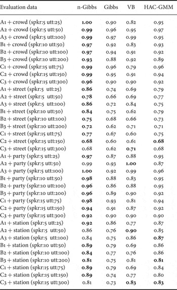
Tables 2 and 3 list the K values obtained using each method for clean and noisy speech data, respectively. These tables demonstrate that the nested Gibbs sampler outperformed the conventional Gibbs sampler irrespective of the evaluation sets, under clean and noisy conditions. These results imply that the proposed method can model data drawn from both single and multi-modal distributions, which the conventional Gibbs sampler was unable to calculate.
K-value for clean test sets.

K value for noisy test sets. Four types of noise (crowd, street, party, and station) are overlapped with speech of nine datasets.
2) Comparison with the VB-based method and agglomerative method
The K values determined using the VB-based and agglomerative methods are also listed in Tables 2 and 3. The results obtained by the proposed method were equal or superior to those with the conventional VB-based (VB) methods using both the clean and noisy datasets. In particular, the proposed method obtained substantially better performance when the data were very scarce (e.g. A1, B1, C1, T1, and T2). This implies that nested Gibbs sampling-based estimation can adequately estimate the cluster structure from limited data, which is generally difficult to achieve. In fact, the VB-based method cannot model such limited data. To evaluate the effectiveness of a fully Bayesian approach, we also compared the proposed method with the conventional hierarchical agglomerative method (HAC-GMM). The proposed method also outperformed the HAC-GMM in most conditions.
3) Computational cost
We now consider the computational cost based on two features: the number of iterations until convergence and the computation required for each epoch. The T-1 dataset (i.e., 24 speakers and 192 utterances; 9.7 min in total) was used for this experiment. The VB approach required about 14.8 s on average for one epoch and 12 iterations until it converged (i.e., real-time factor (RTF) of about 0.0031) when an Intel Xeon 3.00 GHz processor was used. However, the proposed nested Gibbs sampling method required about 41.4 s on average for one epoch and about 63 iterations until the maximum logarithmic marginalized likelihood was obtained (i.e., RTF of about 0.0450), whereas the conventional Gibbs sampling method only required about 1.58 s and about 17 iterations until the maximum logarithmic marginalized likelihood was obtained (i.e., RTF of about 0.0005). Figure 6(a) shows the logarithmic marginalized likelihood obtained when the nested Gibbs sampler was applied to dataset A1. We can see that the chain of samples obtained using the nested Gibbs sampler converged within 100 iterations at most. Compared with the conventional Gibbs sampler, the nested Gibbs sampler required more iterations and computations while it obtains substantially better performance. In fact, the computational cost of the nested Gibbs sampler will increase drastically as the number of utterances increases because many iterations are needed during the sampling process. However, the sampling of fLVs can be parallelized, because the posterior distribution of fLVs is calculated independently of the utterances. Thus, we can reduce the computational time by using multi-threading technology.
VI. CONCLUSION AND FUTURE WORK
In this study, we proposed a novel method for estimating a mixture-of-mixture model. The proposed nested Gibbs sampler can efficiently avoid local optimum solutions due to its nested sampling procedure, where the structure of its elemental mixture distributions are sampled jointly. We showed that the proposed method can estimate models accurately for speech utterances drawn from complex multi-modal distributions, whereas the results obtained by the conventional Gibbs sampler-based method were trapped in local optima. The proposed method also outperformed the conventional agglomerative approach in most conditions.
The proposed MoGMMs can build a hierarchical model from multi-level data that comprise frame-wise observations. Some types of real-world data also has the same kind of structure, such as images comprising a set of pixels. In future research, we plan to apply MoGMMs to the image-clustering problem.
Non-parametric Bayesian approaches have recently been attracting the attention as methods for selecting optimal model structures. For example, the nested Dirichlet process mixture model [Reference Rodriguez and Dunson30] provides a model selection solution for our MoGMMs. In a previous study, we proposed a non-parametric Bayesian version of a mixture-of-mixture model and showed that it was effective in estimating the number of speakers [Reference Tawara, Ogawa, Watanabe, Nakamura and Kobayashi31,Reference Tawara, Ogawa, Watanabe, Nakamura and Kobayashi32]. However, this model was based on the conventional Chinese restaurant process and we employed the conventional Gibbs sampling method, which is readily trapped by the local optima. In future research, we plan to develop a nested Gibbs sampling-based method for such non-parametric Bayesian models.
Appendix
In this appendix, we provide detailed descriptions of how to calculate the posterior probabilities for the fLVs and sLVs in equations (31) and (33), which are required for nested Gibbs sampling. [sLV]
 $$\eqalign{& p(z_{u} = i \vert {\cal O}, {\cal V}_{u}, \lcub {\cal V}_{\backslash u},{\cal Z}_{\backslash u}\rcub ) \cr & \quad = {p({\cal O},{\cal V},{\cal Z}_{\backslash u},z_{u}=i) \over p({\cal O},{\cal V},{\cal Z}_{\backslash u})} \cr & \quad \propto {p({\cal O},{\cal V},{\cal Z}_{\backslash u},z_{u}=i) \over p({\cal O}_{\backslash u}, {\cal V}_{\backslash u}, {\cal Z}_{\backslash u})} \cr & \quad \propto \exp \left\{\log {\Gamma\left(\sum_{j}\tilde{w}_{i\backslash u,j}\right) \over \Gamma \left(\sum_{j}\tilde{w}_{i,j} \right)} \right. \cr & \qquad - \left. \beta \sum_{j} \lpar H(\tilde{{\bf \Psi}}_{i,j}) - H(\tilde{{\bf \Psi}}_{i\backslash u,j})\rpar \right\}\cr & \quad {\mathop{=}\limits^{\Delta}} \gamma_{z_{u}=i \vert {\cal V}}^{\beta}.}$$
To derive the result using equation (37), we assume that the marginalized likelihood for each complete data $\{{\bf o}_{ut}, v_{ut}, z_{u}\}$
is independent from the others, and use the fact that
$\{{\bf o}_{ut}, v_{ut}, z_{u}\}$
is independent from the others, and use the fact that
 $$\eqalign{p({\cal O}, {\cal V}_{u}, \lcub {\cal V}_{\backslash u},{\cal Z}_{\backslash u}\rcub ) &= p({\cal O_{\backslash u}, {\cal V}_{\backslash u}, {\cal Z}_{\backslash u})} \sum_{z_u} p({\cal O}_{u},{\cal V}_{u}, z_{u}) \cr &\propto p({\cal O}_{\backslash u}, {\cal V}_{\backslash u}, {\cal Z}_{\backslash u}),}$$ $H(\tilde{\bf \Psi}_{i,j})$
in equation (37) denotes the logarithmic likelihood of the complete data
$H(\tilde{\bf \Psi}_{i,j})$
in equation (37) denotes the logarithmic likelihood of the complete data $\{{\cal O}, {\cal Z}, {\cal V}\}$
, which is defined as follows:
$\{{\cal O}, {\cal Z}, {\cal V}\}$
, which is defined as follows:
 $$\eqalign{H(\tilde{\bf \Psi}_{i,j}) &{\mathop{=}\limits^{\Delta}} \log p({\cal O}, {\cal V}_{u\backslash t} \lcub {\cal V}_{\backslash u},{\cal Z}_{\backslash u}\rcub , v_{ut} = j,z_{u} = i) \cr &\propto \log \Gamma(\tilde{w}_{ij}) - {D \over 2} \log \tilde{\xi}_{ij} \cr & \quad + D \log \Gamma \left({\tilde{\eta}_{ij} \over 2} \right) - {\tilde{\eta}_{ij} \over 2} \sum\nolimits_{d} \log \tilde{\sigma}_{ij,d,}}$$
where h̃
i
, w̃
ij
, $\tilde{\xi}_{ij}$
,
$\tilde{\xi}_{ij}$
, $\tilde{\eta}_{ij}$
,
$\tilde{\eta}_{ij}$
, $\tilde{\bf \mu}_{ij}$
, and
$\tilde{\bf \mu}_{ij}$
, and $\tilde{\sigma}_{ij,d}$
denote the hyper-parameters of the marginalized likelihood defined in equation (22). We can also obtain the samples of fLVs from these factorized distributions as follows:
[fLVs]
$\tilde{\sigma}_{ij,d}$
denote the hyper-parameters of the marginalized likelihood defined in equation (22). We can also obtain the samples of fLVs from these factorized distributions as follows:
[fLVs]
 $$\eqalign{& p(v_{ut} = j \vert {\cal O}, {\cal V}_{u\backslash t}, \lcub {\cal V}_{\backslash u}, {\cal Z}_{\backslash u}\rcub, z_{u} = i) \cr & \quad = {p({\cal O},{\cal V}_{u\backslash t}, \lcub {\cal V}_{\backslash u}, {\cal Z}_{\backslash u}\rcub , v_{ut} = j, z_{u}=i) \over p({\cal O},{\cal V}_{u\backslash t}, \lcub {\cal V}_{\backslash u}, {\cal Z}_{\backslash u}\rcub , z_{u} = i)} \cr & \quad \propto {p({\cal O},{\cal V}_{u\backslash t}, \lcub {\cal V}_{\backslash u}, {\cal Z}_{\backslash u}\rcub , v_{ut} = j, z_{u}=i) \over p({\cal O}_{\backslash \lcub ut \rcub }, {\cal V}_{\backslash \lcub ut \rcub }, {\cal Z}_{\backslash u},z_{u} = i)} \cr & \quad \propto \exp \lcub -\beta \lpar H(\tilde{\bf \Psi}_{i,j}) - H(\tilde{\bf \Psi}_{i,j\backslash t})\rpar \rcub \cr & \quad {\mathop{=}\limits^{\Delta}} \gamma_{v_{ut}=j \vert z_{u}=i,}^{\beta}}$$
where $H(\tilde{\bf \Psi}_{i{\backslash u},j}) H(\tilde{\bf \Psi}_{i,j{\backslash t}})$
in equations (37) and (40) denote the logarithmic likelihood of complete data with respect to
$H(\tilde{\bf \Psi}_{i{\backslash u},j}) H(\tilde{\bf \Psi}_{i,j{\backslash t}})$
in equations (37) and (40) denote the logarithmic likelihood of complete data with respect to $\{{\cal O}_{\backslash t}, {\cal Z}, {\cal V}_{\backslash t}\}$
and
$\{{\cal O}_{\backslash t}, {\cal Z}, {\cal V}_{\backslash t}\}$
and $\{{\cal O}_{\backslash u}, {\cal Z}_{\backslash u}, {\cal V}_{\backslash u}\}$
, respectively.
$\{{\cal O}_{\backslash u}, {\cal Z}_{\backslash u}, {\cal V}_{\backslash u}\}$
, respectively.
To derive the result equation (40), we assume that the marginalized likelihood for each complete data $\{{\bf o}_{ut}, v_{ut}, z_{u}\}$
is i.i.d. and we use the fact that
$\{{\bf o}_{ut}, v_{ut}, z_{u}\}$
is i.i.d. and we use the fact that
 $$\eqalign{& p({\cal O}, {\cal V}_{u\backslash t}, \lcub {\cal V}_{\backslash u}, {\cal Z}_{\backslash u}\rcub , z_{u}=i) \cr & \quad = p({\cal O}_{\backslash \lcub ut\rcub }, {\cal V}_{\backslash \lcub ut\rcub }, {\cal Z}_{\backslash u},z_{u}=i) \sum_{v_{ut}} p({\bf o}_{ut}, v_{ut}, z_{u}=i) \cr & \quad \propto p({\cal O}_{\backslash \lcub ut \rcub }, {\cal V}_{\backslash \lcub ut \rcub }, {\cal Z}_{\backslash u},z_{u} = i).}$$
Naohiro Tawara received his B.S. and M.S. degrees from Waseda University in Tokyo, Japan in 2010 and 2012. He is currently working as a Research Associate in Waseda University. He is a member of the Acoustical Society of Japan. His research interests include speaker recognition, image processing, and machine learning.
Tetsuji Ogawa received his B.S., M.S., and Ph.D. in electrical engineering from Waseda University in Tokyo, Japan, in 2000, 2002, and 2005. He was a Research Associate from 2004 to 2007 and a Visiting Lecturer in 2007 at Waseda University. He was an Assistant Professor at Waseda Institute for Advanced Study from 2007 to 2012. He has been an Associate Professor at Waseda University and Egypt-Japan University of Science and Technology (E-JUST) since 2012. He was a Visiting Scholar in the Center for Language and Speech Processing, Johns Hopkins University, Baltimore, MD, from June to September in 2012 and from June to August in 2013, and a Visiting Scholar in Speech Processing Group, Faculty of Information Technology, Brno University of Technology, Czech Republic from June to July in 2014 and May to August in 2015. His research interests include stochastic modeling for pattern recognition, speech enhancement, and speech and speaker recognition. He is a member of the Institute for of Electrical and Electronics Engineering (IEEE), Information Processing Society of Japan (IPSJ) and Acoustic Society of Japan (ASJ). He received the Awaya Prize Young Researcher Award from the ASJ in 2011 and Yamashita SIG Research Award from the IPSJ in 2013.
Shinji Watanabe is a Senior Principal Research Scientist at Mitsubishi Electric Research Laboratories (MERL), Cambridge, MA. He received his Ph.D. from Waseda University, Tokyo, Japan, in 2006. From 2001 to 2011, he was a research scientist at NTT Communication Science Laboratories, Kyoto, Japan. From January to March in 2009, he was a visiting scholar in Georgia institute of technology, Atlanta, GA. His research interests include Bayesian machine learning and speech and spoken language processing. He has been published more than 100 papers in journals and conferences, and received several awards including the Best paper award from the IEICE in 2003. He served an Associate Editor of the IEEE Transactions on Audio Speech and Language Processing, and he is a member of several committees including the IEEE Signal Processing Society Speech and Language Technical Committee and the APSIPA Speech, Language, and Audio Technical Committee.
Tetsunori Kobayashi received B.E., M.E., and Dr.E. degrees from Waseda University, Japan, in 1980, 1982, and 1985, respectively. In 1985, he joined Hosei University where he served as a lecturer and then as an associate professor. In 1991, he moved to Waseda University and has been a professor there since 1997. He was a visiting researcher in MIT's Laboratory for Computer Science, Advanced Telecommunication Laboratory, and NHK's Science and Technical Research Laboratory. His research interests include the basics of speech recognition and synthesis and of image processing and applying them to conversational robots.


 Open access