

Introduction
Bed elevation and ice-thickness measurements are routinely collected along flight lines by airborne ice-penetrating radars, which measure the signal travel time from the ice surface to the bed (e.g. Reference GogineniGogineni and others, 2001). These profile measurements are then used to map the ice thickness and bed topography over the entire ice sheet using various methods. Geostatistical techniques, such as kriging (Reference Deutsch and JournelDeutsch and Journel, 1998), are most commonly employed (e.g. Reference Bamber, Layberry and GogineniBamber and others, 2001, Reference Bamber2013; Reference FretwellFretwell and others, 2013). Other approaches based on mass conservation have also been developed (e.g. Reference RasmussenRasmussen, 1988). Contrary to geostatistical techniques, mass-conservation methods rely on additional datasets to interpolate ice-thickness data between flight lines.
Ice-thickness mapping remains challenging in ice-sheet coastal sectors, especially in South Greenland. The presence of englacial water produces volume scattering (Reference SmithSmith and Evans, 1972) and absorption, which greatly reduces the signal strength. Outlet glaciers are also generally located in steep, entrenched, valleys. The geometry of these glaciers creates off-nadir reflections along the side-walls, which makes the bed reflection ambiguous to detect (Reference Holt, Peters, Kempf, Morse and BlankenshipHolt and others, 2006; Reference Wu, Jezek, Rodriguez, Gogineni, Rodriguez-Morales and MoralesWu and others, 2011). Consequently, despite significant effort, including NASA's Operation IceBridge (OIB), ice-thickness data coverage in South Greenland remains suboptimal for conventional mapping methods based on geostatistics. Moreover, ice-thickness measurements are not always consistent between campaigns, and large crossover errors must be dealt with. It is not always clear what measurements must be filtered out, which complicates conventional mapping methods.
Here we present and compare two algorithms based on mass conservation to improve ice-thickness mapping in coastal southern Greenland. Compared to other regions of the ice sheet, South Greenland is also challenging for mass-conservation schemes, because the coverage of ice motion data has gaps that prevent conventional mass-conservation algorithms working, as they require full coverage. We focus here on two basins of South Greenland (Fig. 1): (1) Qooqqup Sermia and Kiattuut Sermiat, located near the southern tip of the Greenland ice sheet (61.28 N, 45.28 W), and (2) Ikertivaq, located on the southeastern coast of Greenland (65.6˚N, 40.0˚W) (Reference Weidick, Williams and FerrignoWeidick, 1995). These two regions represent two settings that are typical for South Greenland. Very few ice-thickness measurements are available in the vicinity of Qooqqup Sermia and Kiattuut Sermiat, but the coverage of ice motion data (Rignot and Mouginot, 2012) is complete, which makes a mass-conservation algorithm reliable. Ikertivaq, by contrast, has been relatively well surveyed, but many gaps remain in the ice motion data. For these two regions, we apply two types of mass-conservation algorithms that are based on the same principle, but apply mass conservation either as a hard constraint (Reference Morlighem, Rignot, Seroussi, Larour, Dhia and DhiaMorlighem and others, 2011) or as a soft constraint. We compare our results against the existing ice-thickness maps of Reference Bamber, Layberry and GogineniBamber and others, 2001, Reference Bamber2013, obtained using a conventional Ordinary-Kriging algorithm. We conclude with recommendations for ice-thickness mapping of glaciers in coastal southern Greenland.
(a, b) Observed surface velocities for (a) Qooqqup Sermia and Kiattuut Sermiat and (b) Ikertivaq (Rignot, 2012). (c, d) OIB thickness lines overlaid on a Moderate Resolution Imaging Spectroradiometer (MODIS) Mosaic of Greenland. The dashed line indicates the limit of the domain where mass conservation is applied. The ice edge and OIB flight lines are shown as solid white lines.

Method
We rely here on the principle of conservation of mass to derive ice-thickness maps, provided that ice motion data and surface accumulation data exist. Bed topography can be deduced by subtracting the calculated ice thickness from an independently gridded digital map of surface elevation.
The first algorithm of ice-thickness mapping based on mass conservation was applied to Columbia Glacier, Alaska (Reference RasmussenRasmussen, 1988). Reference Fastook, Brecher and HughesFastook and others (1995) and Reference Warner and BuddWarner and Budd (2000) employed a similar scheme, but used modeled velocities to map the bed topography of Jakobshavn Isbræ, West Greenland, and the Antarctic ice sheet, respectively. The algorithms that are used here, and described below, are based on the same principle, but account for all measurements of ice-thickness data by relying on optimization (Reference Morlighem, Rignot, Seroussi, Larour, Dhia and DhiaMorlighem and others, 2011, Reference Morlighem2013). We also employ exclusively the newly available observed high-resolution ice motion data, derived from radar interferometry (Rignot and Mouginot, 2012), in order to preserve velocity directions and avoid any problem of circularity, as modeled velocities require prior knowledge of bed topography and ice thickness (Reference MorlighemMorlighem and others, 2013). We therefore neglect vertical shear (i.e. plug flow) in the model domain, which is a reasonable assumption for fast-flowing glaciers but may not be reasonable for slow-moving ice. To validate this assumption, we use a higher-order ice-sheet model (Reference BlatterBlatter, 1995; Reference PattynPattyn, 2003) to calculate the amount of vertical shear. The results show that surface speeds are <4% higher than depth-averaged speeds over the entire domain, Ω, for both glaciers, which is consistent with other fast-flowing glaciers of the Greenland ice sheet (e.g. Reference SeroussiSeroussi and others, 2011; Reference MorlighemMorlighem and others, 2013).
Mass conservation
The equation of mass conservation is based on the depth-integrated continuity equation. The ice thickness, H, must satisfy
where ![]() is the depth-averaged ice velocity and a is the apparent mass balance, i.e. the sum of surface mass balance, basal melting and thinning rate (Reference Morlighem, Rignot, Seroussi, Larour, Dhia and DhiaMorlighem and others, 2011).
is the depth-averaged ice velocity and a is the apparent mass balance, i.e. the sum of surface mass balance, basal melting and thinning rate (Reference Morlighem, Rignot, Seroussi, Larour, Dhia and DhiaMorlighem and others, 2011).
If ![]() and a are provided, either from model outputs or from direct measurements, we can calculate the ice thickness over the entire domain by solving the following hyperbolic problem:
and a are provided, either from model outputs or from direct measurements, we can calculate the ice thickness over the entire domain by solving the following hyperbolic problem:
where Ω is the model domain and Γ_ the inflow boundary, along which ice-thickness measurements, H obs, are required and imposed.
This standard approach yields products that may deviate significantly from the measurements, due to errors in the input data (Reference Morlighem, Rignot, Seroussi, Larour, Dhia and DhiaMorlighem and others, 2011). The only ice-thickness data that constrain the computation of ice thickness in this method are along the inflow boundary, r_.
Here we wish to account for all measurements of ice thickness, H obs, along flight tracks, T, that lie within the model domain, . We therefore formulate an optimization problem, where the following cost function must be minimized:
This minimization is under constraint, as we want the ice thickness, H, to satisfy the mass-conservation equation (Eqn (1)). To do so, we either impose Eqn (2) as a hard constraint or we impose Eqn (1) as a soft constraint.
Hard constraint
When the mass-conservation equation is applied as a hard constraint, we have a PDE (partial differential equation-constrained optimization problem. We minimize J (Eqn (3)) under the constraint provided by Eqn (2). The minimization is achieved by changing the depth-averaged velocity, ![]() , and the apparent mass balance, a, within an interval centered around the observations (±50ma- 1 for ice velocity and ±1 m a-1 for apparent mass balance). The tolerance interval for speed is larger than the nominal error because we must account for differences between surface and depth-averaged velocities, and it gives more flexibility to the optimization process. For the optimization, we rely here on an adjoint-derived gradient descent. This method is described in more detail by Reference Morlighem, Rignot, Seroussi, Larour, Dhia and DhiaMorlighem and others (2011).
, and the apparent mass balance, a, within an interval centered around the observations (±50ma- 1 for ice velocity and ±1 m a-1 for apparent mass balance). The tolerance interval for speed is larger than the nominal error because we must account for differences between surface and depth-averaged velocities, and it gives more flexibility to the optimization process. For the optimization, we rely here on an adjoint-derived gradient descent. This method is described in more detail by Reference Morlighem, Rignot, Seroussi, Larour, Dhia and DhiaMorlighem and others (2011).
This approach is very efficient for fast-flowing regions, where ice motion data are most reliable. In the interior however, ice motion data are closer to the noise level and velocity directions are less accurate.
Soft constraint
For the interior, or for regions with gaps in velocity data, mass conservation can be imposed as a soft constraint. In this case, the mass-conservation equation (Eqn (1)) is added to the cost function, so ice thicknesses that deviate from mass conservation are penalized:
where is a scalar between 0 and 1. Here we do not change the depth-averaged velocity, ⊽, or the apparent mass balance, a. Instead, we optimize the ice thickness, H, directly. This second method is more robust, because errors in input data do not affect the entire domain downstream of these errors but remain localized. It can therefore cope with gaps in velocity data (e.g. by taking 7 = 1 for the regions where velocities are available and 7 = 0 for the locations where there are data gaps). It is also faster, as the mass-conservation equation is never solved and no adjoint state needs to be calculated in order to compute the gradient of the cost function, J, with respect to the ice thickness.
Nevertheless, this algorithm is less satisfactory, because the mass-conservation equation is not exactly fulfilled and fewer features are captured, as shown in the examples below.
Regularization
In order to avoid unrealistic spurious oscillation in ice thickness due to overfitting, it is critical to introduce some regularization to the cost function for both approaches. To do so, we add the following term to the cost function, J:
where n|| is a unit vector parallel to the ice velocity, n is a unit vector perpendicular to the ice velocity and ||, and are constant regularization parameters. The first term penalizes wiggles in ice thickness only in the along-flow direction, while the second term penalizes wiggles across flow. Ice thickness is indeed smoother in the along-flow direction, especially in fast-moving regions. We therefore use || = ± for regions where v < 15 m a-1 and γ|| = 10 7 ± for regions where v≥15ma-1.
Data
Surface mass balance is a product from the regional atmospheric climate model RACMO2 averaged over the time period 1979-2010 (Reference EttemaEttema and others, 2009) at a resolution of 11 km, with errors between 7% and 20% in the ablation zone. The surface mass balance ranges from +1.5 ma-1 in the interior to -1.5 ma-1 at the ice margin for Qooqqup Sermia and Kiattuut Sermiat, and from +1.5 to +4 m a-1 near the ice front of Ikertivaq.
Basal melting under grounded ice is neglected here, and the ice thinning rate is provided by satellite laser altimetry (Ice, Cloud and land Elevation Satellite (ICESat) and Airborne Topographic Mapper (ATM)), at a resolution of 0.10 (Reference Schenk and CsathoSchenk and Csatho, 2012). This dataset provides average thinning rates for the time period 2003-09. Qooqqup Sermia and Kiattuut Sermiat are thickening at a rate of 20 cma-1 in the interior and thinning at 50 cma-1 near the coast. Ikertivaq is experiencing significantly higher thinning rates, from 2 to 10 m a"1 at the margin.
The velocity data are a combination of Japanese Advanced Land Observing Satellite (ALOS) Phased Array-type L-band Synthetic Aperture Radar (PALSAR), RADAR-SAT-1 and Envisat Advanced SAR (ASAR) data (Rignot, 2012), at 150 m spacing, with TerraSAR-X data (Reference Joughin, Smith, Howat, Scambos and ScambosJoughin and others, 2010a,Reference Joughin, Smith, Howat, Scambos and Scambosb) available at 100 m spacing. This dataset covers the period 2008-09. The error associated with this dataset is ~10 m a~1. Bed measurements are from the Center for Remote Sensing of Ice Sheets (CReSIS) (Reference GogineniGogineni, 2012), primarily collected by OIB.
Error quantification
We evaluate the error of the hard constraint algorithm using the error propagation scheme presented by Reference Morlighem, Rignot, Seroussi, Larour, Dhia and DhiaMorlighem and others (2011). Errors between the calculated and measured thicknesses are advected upstream and downstream, and uncertainties in apparent mass-balance and velocity data make this error grow as we move away from flight lines. Here we use an uncertainty in apparent mass balance of δa = 0.5 m a~1, the uncertainty in ice velocity is 2 m a~1 and the uncertainty in strain rate is estimated as 3 x 10⁻⁴a-1, based on observation errors.
Here we adapt this scheme to the soft constraint algorithm by accounting for errors in the mass-conservation constraint, which makes the error grow faster between flight lines. The imbalance in mass conservation is added as a source term in the error propagation scheme, similarly to uncertainties in velocity data or apparent mass balance.
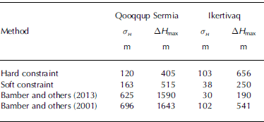
Finally, we quantify the ability of each method to fit ice-thickness measurements, in terms of standard error and maximum error. We compare these errors to those obtained with two other ice-thickness datasets that use Ordinary-Kriging (Reference Bamber, Layberry and GogineniBamber and others, 2001, Reference Bamber2013).
Results
We first focus on the region of Qooqqup Sermia and Kiattuut Sermiat, where the coverage of ice motion data is complete (Fig. 1a). An ice-thickness map was released prior to OIB (Reference Bamber, Layberry and GogineniBamber and others, 2001, Reference Bamber2013) at a horizontal resolution of 5 km (Fig. 2a). The algorithm used to construct this map is based on Ordinary-Kriging (Reference Deutsch and JournelDeutsch and Journel, 1998). The ice thickness is monotonically decreasing as the distance to the coast decreases, despite the presence of two fast ice streams.
Ice thickness of Qooqqup Sermia and Kiattuut Sermiat from (a) Reference Bamber, Layberry and GogineniBamber and others (2001), (b) Reference BamberBamber and others (2013), (c) mass conservation using a hard constraint and (d) mass conservation using a soft constraint. The ice edge and OIB flight lines are shown as solid white lines. The background ice thickness outside the model domain for (c) and (d) is calculated with an Ordinary-Kriging algorithm.

OIB collected ice-thickness data mainly upstream of our model domain (Fig. 1c). There is one crossover that shows inconsistent measurements along Qooqqup Sermia in the center of the model domain. For one line of measurements (TO-2008) the glacier center line shows a deep (1700 m) trough, whereas a second flight line that crosses the glacier (P3-2012) shows a very shallow ice thickness (<100m) and it is not clear from the echograms which measurement is correct.
Bamber and others (2013) used these data to construct an updated product, based again on the algorithm of Ordinary-Kriging (Fig. 2b), at a horizontal resolution of 1 km. More features are apparent in this map, but the ice thickness remains shallow (~50m) along the two ice streams. The data filtering that was applied most likely removed the first flight line (TO-2008). Kriging artifacts are visible along the flight lines, where the ice thickness changes rapidly over small distances.
We apply the two algorithms based on mass conservation to this region, using the same measurements as those used by Reference BamberBamber and others (2013), on an unstructured triangular mesh at a resolution of ~300 m. We first apply the mass-conservation equation as a hard constraint (Fig. 2c). Contrary to the map of Reference BamberBamber and others (2013), this approach yields two narrow and deep troughs (between 700 and 1100m deep).
The algorithm based on a soft constraint also creates a trough for Qooqqup Sermia (Fig. 2d), on the eastern side of the model domain, but the trough is less continuous, as the ice is very shallow (<400m) upstream of the fjord. The trough that coincides with Kiattuut Sermiat on the western side of the model domain is absent when mass conservation is applied as a soft constraint.
The estimated errors (Fig. 3) show that the soft constraint method is indeed less reliable than the hard constraint method, which is expected because the mass-conservation equation is not fully enforced in the soft constraint algorithm. The misfits between radar data and calculated thickness along the flight lines are similar for both methods (Table 1) and four times better than the maps of Reference Bamber, Layberry and GogineniBamber and others, 2001, Reference Bamber2013.
Comparison of errors in ice thicknesses found using the hard constraint and soft constraint mapping methods, taking ice thicknesses given by Bamber and others (2001, 2013) vs the original measurements over the entire domain. H is the standard error and AH max the maximum error
Estimated maximum potential error in ice thickness for the mass-conservation method using (a) a hard constraint and (b) a soft constraint.

In a second application, we focus on Ikertivaq (Fig. 1b). The coverage of ice motion data is not complete in this region, but the region is relatively well surveyed in terms of ice-thickness measurements (Fig. 1d), and crossover errors remain small (<30 m). Similarly to Qooqqup Sermia and Kiattuut Sermiat, prior to OIB the ice thickness is rather featureless, monotonically decreasing toward the ice margin (Fig. 4a; Reference Bamber, Layberry and GogineniBamber and others, 2001).
Ice thickness of Ikertivaq from (a) Reference Bamber, Layberry and GogineniBamber and others (2001), (b) Reference BamberBamber and others (2013), (c) mass conservation using a hard constraint and (d) mass conservation using a soft constraint. The ice edge and OIB flight lines are shown as solid white lines. The background ice thickness outside the model domain for (c) and (d) is calculated with an Ordinary-Kriging algorithm.

The updated dataset of Bamber and others (2013) exhibits a rougher and more complex ice-thickness pattern than the initial one (Fig. 4b), but kriging artifacts are still present along flight lines. When we apply our mass-conservation algorithm with a hard constraint, the algorithm does not converge well and many artifacts are introduced (Fig. 4c). These artifacts coincide exactly with gaps in ice motion data (Fig. 1b). The interpolation that was performed to fill these gaps prevents the algorithm from converging as it introduces erroneous flow directions. The soft constraint algorithm, however, achieves a good convergence with no noticeable artifact in the ice thickness (Fig. 4d).
The error maps (Fig. 5) are consistent with these results: the error associated with the hard constraint map is two to three times larger than that associated with the soft constraint method. The misfits between the soft constraint thickness and measurements along flight lines are similar to the ones obtained by Reference BamberBamber and others (2013) (Table 1), and three times smaller than the hard constraint map.
Estimated maximum potential error in ice thickness for the mass-conservation method using (a) a hard constraint and (b) a soft constraint.

Discussion
Overall, mass-conservation-based algorithms seem to behave better than traditional Ordinary-Kriging in South Greenland, as the coverage of ice-thickness data is sparser than in other regions of coastal Greenland. Important features, such as fjords, troughs, valleys and ridges, are difficult to detect in radar-sounding data, especially in coastal South Greenland. Most of these features are therefore absent from OIB data, and geostatistical techniques are not able to introduce such features, as they solely rely on ice-thickness measurements. Mass-conservation approaches, however, rely on additional information to infer ice thickness between flight lines, which makes them more reliable in regions where very few measurements are available.
The application to Qooqqup Sermia and Kiattuut Sermiat also shows that mass-conservation-based algorithms perform well, even if the number of flight lines along which ice-thickness measurements are collected is limited. It is also clear that, when mass conservation is applied as a strong constraint, more features are captured. The difference between results obtained with the two mass-conservation algorithms is due to the nature of the constraint. When mass conservation is applied as a soft constraint only, the algorithm will tend to gain or lose mass between flight lines, in order to minimize the other terms of the cost function. When mass conservation is applied as a hard constraint, mass is rigorously conserved and elongated features are conserved, even though regularizing terms tend to flatten the ice thickness.
More importantly, mass-conservation algorithms can be used as a validation/filtering tool for the regions where measurements are not reliable. For Qooqqup Sermia, the algorithm shows that, according to the conservation of mass, a deep trough is present. Flight line TO-2008 is therefore correct, and P3-2012 should be discarded. Reference BamberBamber and others (2013) do not keep the right track, which results in a flat bed. Mass-conservation products also provide a reliable first guess, which would greatly help during the processing of echograms, as it indicates where the bed should be, within an error margin of ~100 m, depending on the region.
The application to Ikertivaq demonstrates that full-coverage, high-resolution ice velocity maps are critical to obtain reliable results. As these algorithms are based on a transport equation, they are highly sensitive to velocity directions and to the boundary condition on the inflow boundary, _ (Eqn (2)). As the inflow boundary is located upstream, far from entrenched valleys, it is also the location where ice-thickness measurements are most reliable. Velocity interpolation in data gaps is, however, not a viable option, as it introduces model artifacts in the solution that are advected downstream.
The soft constraint method is able to deal with gaps in velocity data by ignoring the constraint of mass conservation in the locations where no ice velocity is available. In these regions, the algorithm relies solely on regularization constraints, which can prevent elongated features from being captured, as the algorithm will naturally tend to smooth out small-scale details. Soft constrained algorithms are more robust and can be applied when ice velocity coverage is not complete. The solution fit with input radar data along flight lines is similar to Ordinary-Kriging, but the mass-conservation constraint gives additional information between flight lines, whereas kriging relies solely on a weighted average. For bed mapping at the periphery of the Greenland ice sheet, we therefore recommend using hard constrained optimization where possible, and rely on a soft constraint when gaps are present in the velocity data.
Conclusion
Mass-conservation algorithms can be readily applied to South Greenland, despite the relatively low coverage of ice-thickness measurements. We have compared the performance of two algorithms for two regions of South Greenland and shown that algorithms that exactly satisfy the mass conservation better preserve elongated features of glacial origin. However, this approach is highly sensitive to velocity directions, and fails when the coverage of ice motion data is not complete. Soft constrained algorithms are more robust and can be used as an alternative for such regions. Mass-conservation products can be used as a validation tool for regions where ice-thickness measurements are not reliable, and should be used during the data processing, as they provide an initial guess that is based on ice dynamics.
Acknowledgements
This work was performed at the University of California– Irvine, under a contract with the National Aeronautics and Space Administration, Cryospheric Sciences Program, grant NNX12AB86G. We acknowledge the use of data and/or data products from CReSIS generated with support from US National Science Foundation (NSF) grant ANT-0424589 and NASA grant NNX10AT68G.


