


1. Introduction: Taylor–Prandtl controversy
In 1932, G. I. Taylor wrote a fascinating article suggesting that, in two-dimensional (2-D) turbulent flows at least, it is not the momentum of the eddies which is conserved from one step of their random walk to the other (the so-called Reynolds–Prandtl analogy), but their vorticity, and that therefore, the conservation equations (time averaged) for the velocity $u$
and the concentration of a passive scalar
$u$
and the concentration of a passive scalar $c$
must be different. Taylor’s ‘vorticity transport’ theory thus predicts that across a 2-D wake or jet (in the
$c$
must be different. Taylor’s ‘vorticity transport’ theory thus predicts that across a 2-D wake or jet (in the $y$
-direction), the
$y$
-direction), the $u(y)$
profile is exactly related to the
$u(y)$
profile is exactly related to the $c(y)$
profile (when scaled by their maximal value) by
$c(y)$
profile (when scaled by their maximal value) by
 \begin{equation} u=c^2. \end{equation}
The measurements Taylor attributed to Fage and Falkner on this issue (see the Appendix of Taylor Reference Taylor1932) back his audacious, but seemingly relevant proposal. These measurements on the same 2-D wake of a heated bar in air were later confirmed by von Reichardt (Reference von Reichardt1944), who also studied a heated turbulent plane jet to find that (1.1) applies. The same trend, although less pronounced than in (1.1), was observed for the dispersion of heat in a turbulent round air jet by Corrsin (Reference Corrsin1943), and later by So & Hwang (Reference So and Hwang1986) and Darisse, Lemay & Benaïssa (Reference Darisse, Lemay and Benaïssa2013) in the same geometry, as well as for turbulent round plumes (Papanicolaou & List Reference Papanicolaou and List1988; Wang & Law Reference Wang and Law2002), and a jet (Antoine, Lemoine & Lebouché Reference Antoine, Lemoine and Lebouché2001) seeded with rhodamine in water, or a helium jet in air (Salizzoni et al. Reference Salizzoni, Vaux, Creyssels, Amielh, Pietri and Anselmet2023).
All these observations converge towards the same conclusion: the (scaled) average scalar transverse profile $c$
is systematically broader than its axial velocity counterpart
$c$
is systematically broader than its axial velocity counterpart $u$
and we have
$u$
and we have $u\sim c^\beta$
with
$u\sim c^\beta$
with $1\lesssim \beta \lesssim 2$
, a configuration-dependent value.
$1\lesssim \beta \lesssim 2$
, a configuration-dependent value.
1.1. Taylor’s case study: the two-dimensional wake
Inspired by measurements and calculations by Schlichting, Taylor works out (opportunistically, as we will see) the example of the plane wake with velocity deficit $u$
in a uniform stream with velocity
$u$
in a uniform stream with velocity $U$
. To the mean (time-averaged) velocity field
$U$
. To the mean (time-averaged) velocity field $\boldsymbol{u}=\{U-u,v\}$
with vorticity
$\boldsymbol{u}=\{U-u,v\}$
with vorticity $\omega =\boldsymbol{\nabla} \times \boldsymbol{u}= \partial _xv-\partial _yu$
are superimposed zero-mean fluctuating quantities
$\omega =\boldsymbol{\nabla} \times \boldsymbol{u}= \partial _xv-\partial _yu$
are superimposed zero-mean fluctuating quantities $u^{\prime}$
,
$u^{\prime}$
, $v^{\prime}$
and
$v^{\prime}$
and $\omega ^{\prime}=\partial _xv^{\prime}-\partial _yu^{\prime}$
, according to the decomposition going back to Reynolds (Reference Reynolds1895). These random motions mediate the transport of extensities, by a diffusion-like process.
$\omega ^{\prime}=\partial _xv^{\prime}-\partial _yu^{\prime}$
, according to the decomposition going back to Reynolds (Reference Reynolds1895). These random motions mediate the transport of extensities, by a diffusion-like process.
Away from viscous scales, the large-scale equation of motion of a pressure-less flow is $\boldsymbol{u\cdot \nabla u}=\boldsymbol{\nabla} \underline {\sigma }$
with
$\boldsymbol{u\cdot \nabla u}=\boldsymbol{\nabla} \underline {\sigma }$
with $\underline {\sigma }$
a stress tensor (Landau & Lifshitz Reference Landau and Lifshitz1987). For flows with a shallow
$\underline {\sigma }$
a stress tensor (Landau & Lifshitz Reference Landau and Lifshitz1987). For flows with a shallow $x$
-evolution compared with a steeper variation in the
$x$
-evolution compared with a steeper variation in the $y$
-direction (like in jets, boundary layers and wakes), we have
$y$
-direction (like in jets, boundary layers and wakes), we have
 \begin{equation} - U\partial _x u=\partial _y\sigma \quad \textrm {with}\quad \sigma =-\overline {v^{\prime}u^{\prime}} \end{equation}
at the dominant order ( $u, v\ll U$
at large
$u, v\ll U$
at large $x$
), in an incompressible flow with
$x$
), in an incompressible flow with $\partial _xu^{\prime} + \partial _yv^{\prime} = 0$
and where
$\partial _xu^{\prime} + \partial _yv^{\prime} = 0$
and where $\overline {(\boldsymbol{\cdot})}=\lim \limits _{T \rightarrow +\infty }({1}/{T})\int _0^T(\boldsymbol{\cdot})\,\textrm {d}t$
.
$\overline {(\boldsymbol{\cdot})}=\lim \limits _{T \rightarrow +\infty }({1}/{T})\int _0^T(\boldsymbol{\cdot})\,\textrm {d}t$
.
Now comes the fundamental discussion: the existence of a mean free path, or correlation length $\ell$
in the displacement field, is assumed. Within this correlation length, Prandtl (Reference Prandtl1925) further assumes, in full analogy with the kinetics of gases, that the momentum
$\ell$
in the displacement field, is assumed. Within this correlation length, Prandtl (Reference Prandtl1925) further assumes, in full analogy with the kinetics of gases, that the momentum $\rho u^{\prime}$
of eddies is conserved. The transfer of momentum occurs from one fluid layer to the other, each with different mean velocities
$\rho u^{\prime}$
of eddies is conserved. The transfer of momentum occurs from one fluid layer to the other, each with different mean velocities $u(y)$
and a first-order expansion suggests that
$u(y)$
and a first-order expansion suggests that $u^{\prime}\sim \ell \partial _yu$
. Together with the ‘momentum formulation’ of (1.2), we have
$u^{\prime}\sim \ell \partial _yu$
. Together with the ‘momentum formulation’ of (1.2), we have
 \begin{equation} U\partial _x u=\partial _y (\overline {v^{\prime}\ell }\partial _yu )\quad \textrm {according to Prandtl}. \end{equation}
Taylor however emphasises that since vorticity is conserved by motions in a plane, eddies carry their vorticity $\omega ^{\prime}$
as they jump randomly from one layer to the next, where they ‘mix’ with the local ambient vorticity (the merging process is itself far from trivial regarding conservation principles as discussed by Meunier, Le Dizès & Leweke Reference Meunier, Le Dizès and Leweke2005). Equation (1.2) can be rearranged, noticing that
$\omega ^{\prime}$
as they jump randomly from one layer to the next, where they ‘mix’ with the local ambient vorticity (the merging process is itself far from trivial regarding conservation principles as discussed by Meunier, Le Dizès & Leweke Reference Meunier, Le Dizès and Leweke2005). Equation (1.2) can be rearranged, noticing that $u^{\prime}\sim v^{\prime}$
, into
$u^{\prime}\sim v^{\prime}$
, into
 \begin{equation} - U\partial _x u=-\overline {v^{\prime}\omega ^{\prime}}. \end{equation}
Writing again $\omega ^{\prime}=\ell \partial _y\omega$
with
$\omega ^{\prime}=\ell \partial _y\omega$
with $\omega \approx \partial _yu$
the mean background vorticity, we have from the ‘vorticity formulation’ of (1.4),
$\omega \approx \partial _yu$
the mean background vorticity, we have from the ‘vorticity formulation’ of (1.4),
 \begin{equation} U\partial _x u=\overline {v^{\prime}\ell }\partial _y^2u\quad \textrm {according to Taylor}, \end{equation}
which is different from Prandtl’s version. In both cases, the diffusivity ${\mathcal D}=\overline {v^{\prime}\ell }$
needs to be further interpreted, but that separate discussion for the choice of
${\mathcal D}=\overline {v^{\prime}\ell }$
needs to be further interpreted, but that separate discussion for the choice of $\mathcal D$
is distinct from the fundamental fact that depending on the microscopic quantity being conserved (i.e. momentum or vorticity), the macroscopic structure of laws is different. Although, in Taylor’s own words, (1.3) and (1.5)
$\mathcal D$
is distinct from the fundamental fact that depending on the microscopic quantity being conserved (i.e. momentum or vorticity), the macroscopic structure of laws is different. Although, in Taylor’s own words, (1.3) and (1.5)
‘appear at first glance to be very similar’,
the consequence of this difference (the position of the $y$
-derivative), may be significant. This can be particularly appreciated if one wants to apply these (conflicting) ideas to scalar transport: depending on the microscopic dynamics at play, the mean (two-dimensional) concentration field
$y$
-derivative), may be significant. This can be particularly appreciated if one wants to apply these (conflicting) ideas to scalar transport: depending on the microscopic dynamics at play, the mean (two-dimensional) concentration field $c(x,y)$
may be different from the mean velocity field
$c(x,y)$
may be different from the mean velocity field $u(x,y)$
.
$u(x,y)$
.
In this respect, one realises how convenient Taylor’s choice of the wake was, where disturbances are advected at a constant velocity $U$
, to discuss concomitantly the dispersion of scalars. Taking the
$U$
, to discuss concomitantly the dispersion of scalars. Taking the $y$
-derivative of (1.5) indeed leads to
$y$
-derivative of (1.5) indeed leads to
 \begin{equation} U\partial _x\omega =\partial _y ({\mathcal D}\partial _y\omega ), \end{equation}
which is nothing else than a Fourier type of conservation equation for vorticity (see § 5 and Appendix D). Precisely, Taylor also writes, without any explicit justification, an identical conservation equation for the concentration $c$
of a scalar
$c$
of a scalar
 \begin{equation} U\partial _xc=\partial _y ({\mathcal D}\partial _yc ), \end{equation}
fitted with the same dispersion coefficient $\mathcal D$
as for vorticity, expected to be valid whatever the dynamical equation for
$\mathcal D$
as for vorticity, expected to be valid whatever the dynamical equation for $u$
may be (see our critical discussion in § 1.2).
$u$
may be (see our critical discussion in § 1.2).
Let us examine how robust Taylor’s predictions are: in a two-dimensional, momentum-preserving wake (Taylor Reference Taylor1932; Schlichting Reference Schlichting1987), we have
 \begin{equation} u/U\sim x^{-\frac {1}{2}}{\mathcal F}(\xi)\quad \textrm {and}\quad c\sim x^{-\frac {1}{2}}{\mathcal G}(\xi),\end{equation}
which are both functions of the similarity variable $\xi =x^{-({1}/{2})}y$
. Thus,
$\xi =x^{-({1}/{2})}y$
. Thus, $\mathcal D$
writes as a function of the fields
$\mathcal D$
writes as a function of the fields $\mathcal F$
and
$\mathcal F$
and $\mathcal G$
as (
$\mathcal G$
as ( ${\mathcal F}^{\prime}=\textrm {d}{\mathcal F}/\textrm {d}\xi$
)
${\mathcal F}^{\prime}=\textrm {d}{\mathcal F}/\textrm {d}\xi$
)
 \begin{equation} \begin{aligned} {\mathcal D}&=\frac {\xi {\mathcal F}}{2{\mathcal F}^{\prime}}\quad \textrm {following Prandtl},\\ {\mathcal D}&=\frac {(\xi {\mathcal F})^{\prime}}{2{\mathcal F}^{\prime\prime}}\quad \textrm {following Taylor},\\ \textrm {and}\quad {\mathcal D}&=\frac {\xi {\mathcal G}}{2{\mathcal G}^{\prime}}\quad \textrm {from the equation for }c. \end{aligned} \end{equation}
Obviously, a Prandtl momentum transfer theory, with equations structurally identical for $u$
and
$u$
and $c$
, will lead to
$c$
, will lead to ${\mathcal F}= {\mathcal G}$
whatever
${\mathcal F}= {\mathcal G}$
whatever $\mathcal D$
may be, a feature which can be interpreted as being an avatar of the Reynolds analogy: since the objects carrying momentum and mass are identical (the eddies), so are the
$\mathcal D$
may be, a feature which can be interpreted as being an avatar of the Reynolds analogy: since the objects carrying momentum and mass are identical (the eddies), so are the $u$
- and
$u$
- and $c$
-fields.
$c$
-fields.
When the microscopic dynamics ruling $u$
and
$u$
and $c$
are different, which is Taylor’s point of view, we may expect non-trivial differences. We get from (1.9) in that case
$c$
are different, which is Taylor’s point of view, we may expect non-trivial differences. We get from (1.9) in that case
 \begin{equation} \frac {{\mathcal G}^{\prime}}{{\mathcal G}}=\frac {\xi {\mathcal F}^{\prime\prime}}{(\xi {\mathcal F})^{\prime}}, \end{equation}
meaning that the $c$
-field (namely
$c$
-field (namely $\mathcal G$
) is a function of the
$\mathcal G$
) is a function of the $u$
-field (given by
$u$
-field (given by $\mathcal F$
), but not necessarily identical to it. They are identical in the special case
$\mathcal F$
), but not necessarily identical to it. They are identical in the special case ${\mathcal F}\sim 1-k\xi ^2$
, which may not be compatible with the solution of the equation of motion, constraining
${\mathcal F}\sim 1-k\xi ^2$
, which may not be compatible with the solution of the equation of motion, constraining $\mathcal F$
for a given form of
$\mathcal F$
for a given form of $\mathcal D$
. For instance, Taylor uses a mixing length form
$\mathcal D$
. For instance, Taylor uses a mixing length form ${\mathcal D}=\ell ^2\partial _yu$
with
${\mathcal D}=\ell ^2\partial _yu$
with $\ell =ax^{1/2}$
for a wake, giving
$\ell =ax^{1/2}$
for a wake, giving ${\mathcal D}=- a^2{\mathcal F}^{\prime}$
and finds, from the expression of
${\mathcal D}=- a^2{\mathcal F}^{\prime}$
and finds, from the expression of $\mathcal D$
given by the equation of motion in (1.9),
$\mathcal D$
given by the equation of motion in (1.9),
 \begin{equation} \begin{aligned} {\mathcal F}&= \big(1-\xi ^{\frac {3}{2}} \big)^2,\quad \textrm {giving from (1.10)},\quad {\mathcal{G}}= 1-\xi ^{\frac {3}{2}},\\ \textrm {so that}\quad {\mathcal{F}}&= {\mathcal{G}}^2\quad \textrm {in that particular case}. \end{aligned} \end{equation}
More generally, if ${\mathcal F}\sim 1-k\xi ^\alpha$
, then (1.10) shows that
${\mathcal F}\sim 1-k\xi ^\alpha$
, then (1.10) shows that ${\mathcal F}= {\mathcal G}^{{1}/({\alpha -1})}$
.
${\mathcal F}= {\mathcal G}^{{1}/({\alpha -1})}$
.
If the dispersion coefficient is now given by a local Boussinesq form ${\mathcal D}=u\ell$
(see Appendix C and Villermaux Reference Villermaux2025), because
${\mathcal D}=u\ell$
(see Appendix C and Villermaux Reference Villermaux2025), because $U-(U-u)$
is the velocity contrast between the wake and the outside flow, giving
$U-(U-u)$
is the velocity contrast between the wake and the outside flow, giving ${\mathcal D}=a{\mathcal F}$
, then one finds that
${\mathcal D}=a{\mathcal F}$
, then one finds that
 \begin{equation} {\mathcal F}\sim 1-\frac {\xi ^2}{4a}, \end{equation}
holding for both the Prandtl and Taylor versions of the equation of motion, as before, but now leading to ${\mathcal F}={\mathcal G}$
, in this other particular case.
${\mathcal F}={\mathcal G}$
, in this other particular case.
1.2. Turbulent plane jet
Another way to test Taylor’s vision against experimental facts is to apply the same reasoning to a turbulent plane jet of momentum flux (per unit span-wise length and mass) $m$
and initial thickness
$m$
and initial thickness $h$
. In that case, the
$h$
. In that case, the $u$
- and
$u$
- and $c$
-fields are both Gaussians of the reduced variable
$c$
-fields are both Gaussians of the reduced variable $\xi =y/x$
, and (1.1) applies, whatever the nature of the scalar may be (see § 2). We envisage that the dispersion coefficients
$\xi =y/x$
, and (1.1) applies, whatever the nature of the scalar may be (see § 2). We envisage that the dispersion coefficients $\mathcal{D}_\omega$
and
$\mathcal{D}_\omega$
and $\mathcal{D }_\star$
for vorticity and concentration may be different. The mean equations for these quantities are given by (see also § 3.2)
$\mathcal{D }_\star$
for vorticity and concentration may be different. The mean equations for these quantities are given by (see also § 3.2)
 \begin{align} u\partial _x \omega + v\partial _y \omega &= \partial _y (\mathcal{D}_\omega \partial _y \omega),\end{align}
 \begin{align} u\partial _x c + v \partial _y c &= \partial _y (\mathcal{D }_\star \partial _y c), \end{align}
the question being to know whether the experimental profiles for $u$
and
$u$
and $c$
can be obtained for the same (possibly
$c$
can be obtained for the same (possibly $\xi$
-dependent) diffusivities i.e. for
$\xi$
-dependent) diffusivities i.e. for $\mathcal{D}_\omega =\mathcal{D }_\star$
((1.6) and (1.7), one of Taylor’s premisses), or not.
$\mathcal{D}_\omega =\mathcal{D }_\star$
((1.6) and (1.7), one of Taylor’s premisses), or not.
We seek for a self-similar solution (whose validity has been questioned by Cafiero & Vassilicos Reference Cafiero and Vassilicos2019, but this is a separate discussion) involving a stream function $\{u,v\}=\{\partial _y\psi,-\partial _x\psi \}$
with
$\{u,v\}=\{\partial _y\psi,-\partial _x\psi \}$
with $\psi (\xi)=(m\,x)^{1/2}\,{\mathcal F}(\xi)$
as (Schlichting Reference Schlichting1987)
$\psi (\xi)=(m\,x)^{1/2}\,{\mathcal F}(\xi)$
as (Schlichting Reference Schlichting1987)
 \begin{equation} u=(m/x)^{1/2}\,{\mathcal F}^{\prime} \quad \textrm {and}\quad v=(m/x)^{1/2} (\xi {\mathcal F}^{\prime}-{\mathcal F}/2 ), \end{equation}
with a mean vorticity given by
 \begin{equation} \omega =(m/x^3)^{1/2} \big({\mathcal F}/4-\xi {\mathcal F}^{\prime}-(1+\xi ^2){\mathcal F}^{\prime\prime} \big). \end{equation}
The vorticity equation (1.13) for a plane turbulent jet is thus
 \begin{equation} 3\xi ({\mathcal F} {\mathcal F}^{\prime})^{\prime} + (1+\xi ^2) (3{\mathcal F}^{\prime}{\mathcal F}^{\prime\prime}+{\mathcal F} {\mathcal F}^{\prime\prime\prime}) = \left [\frac {-2 \mathcal{D}_\omega }{(m\,x)^{1/2}} \left (\frac {3 {\mathcal F}^{\prime}}{4}+ 3\xi {\mathcal F}^{\prime\prime} +(1+\xi ^2) {\mathcal F}^{\prime\prime\prime}\right)\right]^{\prime}. \end{equation}
The mean concentration profile has a self-similar solution now involving ${\mathcal G}(\xi)$
as
${\mathcal G}(\xi)$
as
 \begin{equation} c= (h/x)^{1/2} \ {\mathcal G}. \end{equation}
Introducing (1.15) and (1.18) into (1.14) leads to a differential equation
 \begin{equation} - \frac {\sqrt {m h}}{2 x^2} ( \mathcal{F}^{\prime} \mathcal{G} + \mathcal{F} \mathcal{G}^{\prime} )= \frac {1}{x^2} \sqrt {\frac {h}{x}} (\mathcal{D}_\star G^{\prime} ) ^{\prime}, \end{equation}
which can be integrated on $\xi$
to give
$\xi$
to give
 \begin{equation} {\mathcal F} {\mathcal G} = - 2 \frac {\mathcal{D}_\star }{(m\,x)^{1/2}} \, {\mathcal G}^{\prime} \end{equation}
with a zero integration constant since $\mathcal G$
and
$\mathcal G$
and ${\mathcal G}^{\prime}$
vanish far from the jet. Although (1.13) and (1.14) have no simple analytic form (and have fairly, but not exactly, Gaussian solutions), it is possible to discuss the relative widths of the
${\mathcal G}^{\prime}$
vanish far from the jet. Although (1.13) and (1.14) have no simple analytic form (and have fairly, but not exactly, Gaussian solutions), it is possible to discuss the relative widths of the $u$
- and
$u$
- and $c$
-fields on hand of expansions of
$c$
-fields on hand of expansions of $\mathcal F$
and
$\mathcal F$
and $\mathcal G$
about
$\mathcal G$
about $\xi =0$
. Since
$\xi =0$
. Since $\mathcal G$
is even,
$\mathcal G$
is even, ${\mathcal G}^{\prime}$
can be approximated by
${\mathcal G}^{\prime}$
can be approximated by $\xi {\mathcal G}^{\prime\prime}\vert _{\xi =0}$
such that the diffusivity of the concentration is simply equal to (we approximate the odd function
$\xi {\mathcal G}^{\prime\prime}\vert _{\xi =0}$
such that the diffusivity of the concentration is simply equal to (we approximate the odd function ${\mathcal F}(\xi)$
, vanishing in
${\mathcal F}(\xi)$
, vanishing in $\xi =0$
, by
$\xi =0$
, by $\xi {\mathcal F}^{\prime}_0$
)
$\xi {\mathcal F}^{\prime}_0$
)
 \begin{equation} \mathcal{D}_\star \vert _{\xi =0} = (m\,x)^{1/2} \ {\mathcal F}^{\prime}_0\ a_\star, \end{equation}
where the width (in units of $\xi$
) of the concentration profile is
$\xi$
) of the concentration profile is $2a_\star =- {\mathcal G}/{\mathcal G}^{\prime\prime}\vert _{\xi =0}$
.
$2a_\star =- {\mathcal G}/{\mathcal G}^{\prime\prime}\vert _{\xi =0}$
.
For a Gaussian (see § 2) velocity profile such that ${\mathcal F}^{\prime}(\xi) = {\mathcal F}^{\prime}_0 \exp (- \xi ^2/4 a)$
, the same approximations about
${\mathcal F}^{\prime}(\xi) = {\mathcal F}^{\prime}_0 \exp (- \xi ^2/4 a)$
, the same approximations about $\xi =0$
lead, from (1.13), to
$\xi =0$
lead, from (1.13), to
 \begin{equation} \mathcal{D}_\omega \vert _{\xi =0} = (m\,x)^{1/2} \ {\mathcal F}^{\prime}_0\ a\ \frac { 8-12 a}{6+(2-3a)a/a_\omega - 35a},\end{equation}
with $\mathcal{D}_\omega$
an even function so that
$\mathcal{D}_\omega$
an even function so that $\mathcal{D}^{\prime}_\omega \vert _{\xi =0}$
is approximated by
$\mathcal{D}^{\prime}_\omega \vert _{\xi =0}$
is approximated by $\xi \mathcal{D}^{\prime\prime}_\omega \vert _{\xi =0}$
. The width of the vorticity diffusivity profile is such that
$\xi \mathcal{D}^{\prime\prime}_\omega \vert _{\xi =0}$
. The width of the vorticity diffusivity profile is such that $2a_\omega =- \mathcal{D}_\omega /\mathcal{D}^{\prime\prime}_\omega \vert _{\xi =0}$
.
$2a_\omega =- \mathcal{D}_\omega /\mathcal{D}^{\prime\prime}_\omega \vert _{\xi =0}$
.
Assuming, following Taylor, that the diffusivities $\mathcal{D}_\star$
and
$\mathcal{D}_\star$
and $\mathcal{D}_\omega$
are equal, (1.22) and (1.21) imply a relation between the variances
$\mathcal{D}_\omega$
are equal, (1.22) and (1.21) imply a relation between the variances $a$
,
$a$
, $a_\star$
and
$a_\star$
and $a_\omega$
. For
$a_\omega$
. For $a=0.007$
, which is suited to experiments in plane jets (see § 2 and figure 2
a), we have
$a=0.007$
, which is suited to experiments in plane jets (see § 2 and figure 2
a), we have $a_\star /a=1.024$
for
$a_\star /a=1.024$
for $a_\omega =a$
and
$a_\omega =a$
and $a_\star /a\to 1.37$
for
$a_\star /a\to 1.37$
for $a_\omega \to \infty$
(i.e. for a constant diffusivity
$a_\omega \to \infty$
(i.e. for a constant diffusivity $\mathcal{D}_\omega$
, independent of
$\mathcal{D}_\omega$
, independent of $\xi$
), in contradiction with experiments which all show that
$\xi$
), in contradiction with experiments which all show that $a_\star /a=2$
.
$a_\star /a=2$
.
The above mentioned simple example demonstrates that self-similar concentration and vorticity profiles cannot, in contrast to Taylor’s premise, be solutions of the same equations with the same turbulent diffusivity in a plane jet.
1.3. Summary and outstanding questions
We can, at this point, summarise:
-
(i) Taylor’s ‘vorticity transport theory’ is only markedly different from Prandtl’s ‘momentum transport’ model in very specific cases. The relation $u= c^2$
is no more a universal truth than
$u= c$
is, since each rely on a particular functional choice of the dispersion coefficient
$\mathcal D$
. The initial success of this theory is due to the opportunistic choice of the 2-D wake and particular modelling for
$\mathcal D$
;
$u= c^2$
is no more a universal truth than
$u= c$
is, since each rely on a particular functional choice of the dispersion coefficient
$\mathcal D$
. The initial success of this theory is due to the opportunistic choice of the 2-D wake and particular modelling for
$\mathcal D$
; -
(ii) there is, however, an empirical universal truth: in free shear flows (wakes, plane and round jets), the
$c$
-field is systematically either identical to or broader than the
$u$
-field. One could arguably claim that the difference between the
$u$
- and
$c$
-fields is precisely an opportunity to test the validity of one model of transport over the other (i.e. the model for
$\mathcal D$
). That would be true if the amplitude of the difference was not, also, dependent on the molecular diffusion of the scalar (
$Sc=\nu /D$
): in a turbulent round jet,
$u= c$
for
$Sc\gg 1$
, and
$u=c^{1.5}$
for
$Sc=1$
(§ 2); -
(iii) one criticism against the ‘vorticity transport theory’, first formulated by Taylor himself, is that it only applies in two dimensions, not to three-dimensional (3-D) flows, in general. Vorticity is not conserved in three dimensions (circulation is, as well as helicity, as emphasised by Moreau Reference Moreau1961). One could nevertheless argue that shear instabilities often present a large-scale 2-D coherence (this is, in particular, true for a plane jet) despite the more isotropic character of smaller scales. This thus appears as a mild criticism;
-
(iv) Taylor’s vision is, in two dimensions, at odds with the Reynolds momentum transport mechanism at the root of Prandtl’s mixing length theory. Because (1.5) and (1.7) are different, it is, also, at odds with Reynolds’ analogy stating that momentum and mass are carried by the same objects in a turbulent flow (Reynolds Reference Reynolds1874). The most concerning aspect of this theory is the use of the same dispersion coefficient
$\mathcal D$
for both
$\omega$
and
$c$
, and of a transport equation different for
$u$
, but with the same
$\mathcal D$
.


Taylor’s proposal invites to reconsider the form of transport laws in turbulence, the role of the nature of the extensity being transported and of the flow dimensionality. We reexamine these questions on hand of new dedicated experiments and perspective.
Jets seeded with either smoke in air ( $Sc=1$
) or fluorescein in water (
$Sc=1$
) or fluorescein in water ( $Sc=2000$
). First row: Plane jets, instantaneous cross-sections with (a) smoke, (
$Sc=2000$
). First row: Plane jets, instantaneous cross-sections with (a) smoke, ( $h=1\,\textrm{cm}$
,
$h=1\,\textrm{cm}$
, ${Re}=2500$
); (b) fluorescein (
${Re}=2500$
); (b) fluorescein ( $h=2\,\textrm{mm}$
,
$h=2\,\textrm{mm}$
, ${Re}=1400$
); (c) average fluorescein field of panel (b) and sketch of the average axial velocity
${Re}=1400$
); (c) average fluorescein field of panel (b) and sketch of the average axial velocity $u$
and concentration
$u$
and concentration $c$
profiles. Second row: Round jet with (d) smoke, (
$c$
profiles. Second row: Round jet with (d) smoke, ( $d=1\,\textrm{cm}$
,
$d=1\,\textrm{cm}$
, ${Re}=2100$
), (e) fluorescein (
${Re}=2100$
), (e) fluorescein ( $d=4\,\textrm{mm}$
,
$d=4\,\textrm{mm}$
, ${Re}=5000$
) and ( f) average fluorescein field of panel (e).
${Re}=5000$
) and ( f) average fluorescein field of panel (e).

2. Experiments with plane and round jets
The experiments are relatively simple and very classical. They consist in letting a round jet issue at velocity $u_0$
through a tube of diameter
$u_0$
through a tube of diameter $d$
into a large tank filled with the same fluid at rest, and follow the dilution process of a fluorescent dye (fluorescein), or smoke by shinning a plane laser sheet, containing its axis, through the jet (see e.g. van Dyke Reference van Dyke1982; Dimotakis, Miake-Lye & Papantoniou Reference Dimotakis, Miake-Lye and Papantoniou1983; Dimotakis & Catrakis Reference Dimotakis and Catrakis1999 for an early use of this method). The same method is used with plane jets, where the dyed fluid is injected through a slit of width
$d$
into a large tank filled with the same fluid at rest, and follow the dilution process of a fluorescent dye (fluorescein), or smoke by shinning a plane laser sheet, containing its axis, through the jet (see e.g. van Dyke Reference van Dyke1982; Dimotakis, Miake-Lye & Papantoniou Reference Dimotakis, Miake-Lye and Papantoniou1983; Dimotakis & Catrakis Reference Dimotakis and Catrakis1999 for an early use of this method). The same method is used with plane jets, where the dyed fluid is injected through a slit of width $h$
, and the laser sheet shines perpendicular to it.
$h$
, and the laser sheet shines perpendicular to it.
In all cases, the Reynold number ${Re}=u_0h/\nu$
or
${Re}=u_0h/\nu$
or $u_0d/\nu$
is large, of the order of
$u_0d/\nu$
is large, of the order of $10^3$
to
$10^3$
to $10^4$
. The Schmidt number is
$10^4$
. The Schmidt number is $Sc=\nu /D\approx 2000$
for fluorescein in water, meaning that the Péclet number
$Sc=\nu /D\approx 2000$
for fluorescein in water, meaning that the Péclet number $\textit{Pe}={Re}\, Sc$
is very large. The corresponding conditions are summarised in figure 1 and table 1.
$\textit{Pe}={Re}\, Sc$
is very large. The corresponding conditions are summarised in figure 1 and table 1.
The same experiments as with fluorescein in water were replicated with jets of fine mist diluted in air. The smoke particles, produced by an oil smoke generator, are small condensation nuclei for the water vapour contained in air, and the resulting aggregates have sizes ranging from approximately 10 microns down to molecular sizes (Flagan Reference Flagan1998), with particles being proportionally more numerous as their size is smaller. The smoke is an effective gas, with Schmidt number of order unity ( $Sc\approx 1$
); it is visualised through a plane laser sheet as well, by simple Mie scattering, the net reflected intensity being, when the smoke is dilute enough, proportional to the local volume concentration of the mist (van de Hulst Reference van de Hulst1981).
$Sc\approx 1$
); it is visualised through a plane laser sheet as well, by simple Mie scattering, the net reflected intensity being, when the smoke is dilute enough, proportional to the local volume concentration of the mist (van de Hulst Reference van de Hulst1981).
Summary of the different geometries (plane or round), flow conditions (Reynolds number ${Re}$
) and scalars (
${Re}$
) and scalars ( $Sc=\nu /D$
) explored in this study.
$Sc=\nu /D$
) explored in this study.

The fields are then recorded using a fast camera (allowing for particle image velocimetry (PIV) measurements) which, once properly calibrated in intensity, provides movies of instantaneous, time-resolved 2-D slices through the jets scalar fields (figure 1). Various local and global measurements are then made, the extraction of the mean transverse velocity field $u$
and mean concentration or scalar probability of presence field
$u$
and mean concentration or scalar probability of presence field $c$
in the first place (figure 2). The displacement fields are computed using the PIV algorithm of Meunier & Leweke (Reference Meunier and Leweke2003b
) either by using the high-
$c$
in the first place (figure 2). The displacement fields are computed using the PIV algorithm of Meunier & Leweke (Reference Meunier and Leweke2003b
) either by using the high- $Sc$
field as a tracer or using seeded tracer particles, the two methods providing identical results (see Appendix A). The
$Sc$
field as a tracer or using seeded tracer particles, the two methods providing identical results (see Appendix A). The $c$
-field is obtained by averaging the movie frames.
$c$
-field is obtained by averaging the movie frames.
Transverse (along $y$
or
$y$
or $r$
) concentration (black) profiles
$r$
) concentration (black) profiles $c$
and velocity (blue) profiles
$c$
and velocity (blue) profiles $u$
normalised by their maximal value. Both raw profiles (left, lin-lin units) and rescaled profiles according to
$u$
normalised by their maximal value. Both raw profiles (left, lin-lin units) and rescaled profiles according to $u=c^\beta$
(right, log-lin units) are shown. The red continuous lines are Gaussian fits
$u=c^\beta$
(right, log-lin units) are shown. The red continuous lines are Gaussian fits $e^{-\xi ^2/4a}$
(with
$e^{-\xi ^2/4a}$
(with $\xi =y/x=(y/h)/(x/h)$
). (a) Smoke plane jet in air (
$\xi =y/x=(y/h)/(x/h)$
). (a) Smoke plane jet in air ( $Sc= 1$
) at
$Sc= 1$
) at $x/h=60$
, rescaling
$x/h=60$
, rescaling $u=c^{2}$
. The red dotted line is Schlichting’s formula
$u=c^{2}$
. The red dotted line is Schlichting’s formula $1-\tanh ^2({\xi }/{2\sqrt {a}})$
with same variance as the Gaussian. (b) Fluorescein plane water jet (
$1-\tanh ^2({\xi }/{2\sqrt {a}})$
with same variance as the Gaussian. (b) Fluorescein plane water jet ( $Sc=2000$
) at
$Sc=2000$
) at $x/h=47$
, rescaling
$x/h=47$
, rescaling $u=c^{2}$
. (c) Smoke round jet in air (
$u=c^{2}$
. (c) Smoke round jet in air ( $Sc= 1$
) at
$Sc= 1$
) at $x/d=55$
, rescaling
$x/d=55$
, rescaling $u=c^{1.5}$
. The red dotted line is Schlichting’s formula
$u=c^{1.5}$
. The red dotted line is Schlichting’s formula $(1+{\xi ^2}/{8a})^{-2}$
with same variance as the Gaussian. (d) Fluorescein round water jet (
$(1+{\xi ^2}/{8a})^{-2}$
with same variance as the Gaussian. (d) Fluorescein round water jet ( $Sc=2000$
) at
$Sc=2000$
) at $x/d=90$
, rescaling
$x/d=90$
, rescaling $u=c^{1}$
.
$u=c^{1}$
.

Experiments display a curious, contrasted landscape: there is a qualitative difference between plane and round jets. The former are insensitive to the nature of the dye being transported, while the latter are not. In plane jets, the $c$
-field is systematically broader than the
$c$
-field is systematically broader than the $u$
-field, whatever
$u$
-field, whatever $Sc$
may be, while in round jets,
$Sc$
may be, while in round jets, $u$
- and
$u$
- and $c$
-fields are identical at
$c$
-fields are identical at $Sc=2000$
, but
$Sc=2000$
, but $c$
is broader than
$c$
is broader than $u$
when
$u$
when $Sc=1$
, a feature already noticed explicitly by Corrsin (Reference Corrsin1943) in a heated jet (where
$Sc=1$
, a feature already noticed explicitly by Corrsin (Reference Corrsin1943) in a heated jet (where $Sc\equiv \nu /\kappa ={\mathcal O}(1)$
, with
$Sc\equiv \nu /\kappa ={\mathcal O}(1)$
, with $\kappa$
the diffusivity of heat, see figure 3
a). Our observations are (
$\kappa$
the diffusivity of heat, see figure 3
a). Our observations are ( $\xi =y/x\,\,\textrm {and}\,\, r/x$
in plane and round jets, respectively)
$\xi =y/x\,\,\textrm {and}\,\, r/x$
in plane and round jets, respectively)
 \begin{equation} \begin{aligned} u\sim e^{-\frac {\xi ^2}{4a}}\,\,\textrm {and}\,\, c&\sim e^{-\frac {\xi ^2}{4a_\star }},\,\,\textrm {with}\\ a_\star &=2a=0.014\quad \textrm { for a plane jet at all } Sc,\\ a_\star &=a=0.004\quad \textrm { for a round jet at } Sc=2000\\ \textrm {and}\quad a_\star &\approx 1.5\,a=0.006\quad \textrm {for a round jet at } Sc=1. \end{aligned} \end{equation}
These trends are robust, independent of the axial location in the jets, as seen in figure 3(b). In all cases however, both the $u$
- and
$u$
- and $c$
-profiles are well fitted by a Gaussian, even on the more stringent log-scale compared with the lin-lin scaling routinely used in this context (see Appendix A).
$c$
-profiles are well fitted by a Gaussian, even on the more stringent log-scale compared with the lin-lin scaling routinely used in this context (see Appendix A).
A point of terminology: The flow behind a straight rod is called a 2-D wake, the jet issuing from a slit is a 2-D jet and the flow from a round orifice is a jet in three dimensions. However, the expansion of a wake or plane jet in 2-D is due to to a one-dimensional (1-D) entrainment process (along the direction $y$
in figure 1), and that of a 3-D jet due to a 2-D process (in the plane with radial coordinate
$y$
in figure 1), and that of a 3-D jet due to a 2-D process (in the plane with radial coordinate $r$
in figure 1). An impulsive puff expands in 3-D through a 3-D dispersion process (see § 4.1).
$r$
in figure 1). An impulsive puff expands in 3-D through a 3-D dispersion process (see § 4.1).
These observations indicate the existence of an intricate coupling between the geometry of the flow (plane or round), possibly related to the dimensionality of the entrainment process involved in each case (1-D in a plane jet, axi-symmetrical 2-D in a round jet), and the diffusive properties of the scalar being transported (Sc plays an intrinsic role in round jets). The problem is all the more interesting that the origin of these differences has to be sought for within a universal frame for dispersion where all the profiles, in any condition, are close to Gaussian.
We will, to untangle this web of constraints, proceed step by step, starting back to the basics of turbulent dispersion.
Transverse (versus r/d) concentration (c, black) and velocity (u, blue) profiles in round jets. Red lines are fits by a Gaussian as in (2.1). (a) Corrsin’s measurements in a heated round $d=1$
inch air jet (Corrsin Reference Corrsin1943) in (i)
$d=1$
inch air jet (Corrsin Reference Corrsin1943) in (i) $x/d=10$
and (ii)
$x/d=10$
and (ii) $x/d=20$
both rescaled by
$x/d=20$
both rescaled by $u=c^{1.5}$
. (b) Fluorescein round jet in water (
$u=c^{1.5}$
. (b) Fluorescein round jet in water ( $Sc=2000$
) at
$Sc=2000$
) at ${Re}=5000$
in (from bottom to top)
${Re}=5000$
in (from bottom to top) $x/d= 15,\, 30,\, 50$
, all rescaled according to u = c (velocity and concentration profiles are identical).
$x/d= 15,\, 30,\, 50$
, all rescaled according to u = c (velocity and concentration profiles are identical).

3. Conservation laws and useful relations in turbulent jets
We first recall conservation laws and axial dependences of averages in high Reynolds, momentum-driven jets, and then derive important relations between fluctuations and averages in shear flows.
3.1. Conservation laws
We call $u_0$
and
$u_0$
and $c_0$
the injection velocity and concentration of a stream injected through a slit of thickness
$c_0$
the injection velocity and concentration of a stream injected through a slit of thickness $h$
(plane jet) or nozzle with diameter
$h$
(plane jet) or nozzle with diameter $d$
(round jet), and
$d$
(round jet), and $R$
the transverse width or radius of the resulting stationary jet at a downstream location
$R$
the transverse width or radius of the resulting stationary jet at a downstream location $x$
, where the (cross-section averaged) axial velocity and concentration are
$x$
, where the (cross-section averaged) axial velocity and concentration are $\mathbb{u}$
and
$\mathbb{u}$
and $\mathbb{c}$
. Jets are injected in a quiescent environment of the same fluid at
$\mathbb{c}$
. Jets are injected in a quiescent environment of the same fluid at $u=c=0$
.
$u=c=0$
.
Far downstream from the injection region ( $x\gg h, d$
),
$x\gg h, d$
), $R$
and
$R$
and $\mathbb{u}$
are the only length and velocity scales. Self-similarity and axial momentum flux conservation provide the well-known relations for the means in turbulent jets (see Appendix B):
$\mathbb{u}$
are the only length and velocity scales. Self-similarity and axial momentum flux conservation provide the well-known relations for the means in turbulent jets (see Appendix B):
-
Plane jet. Axial momentum flux (per unit span-wise length and mass)
$m \sim {\mathbb{u}}^2R$
and scalar flux conservation
$u_0hc_0\sim {\mathbb{u}}R{\mathbb{c}}$
provide(3.1)Average velocity and concentration decay like
\begin{align} {\mathbb{u}}/u_0={\mathbb{c}}/c_0\sim (h/R)^{1/2}\quad \textrm {and}\quad R\sim x.\end{align}
$x^{-1/2}$
. The dispersion coefficient
${\mathcal D}={\mathbb{u}}R$
increases like the axial flow-rate as
$u_0(hx)^{1/2}$
.
-
Round jet. Axial momentum flux
$m \sim {\mathbb{u}}^2R^2$
and scalar flux conservation
$u_0d^2c_0\sim {\mathbb{u}}R^2{\mathbb{c}}$
provide(3.2)Average velocity and concentration decay like
\begin{align} {\mathbb{u}}/u_0={\mathbb{c}}/c_0\sim d/R\quad \textrm {and}\quad R= \alpha \, x\; \textrm {(with pre-factor } \alpha \approx 1/6, \textrm { see Appendix B)}.\end{align}
$x^{-1}$
as a consequence of the increase of the volume flow-rate carried by the jet
$Q\sim {\mathbb{u}}R^2\sim u_0\, \textrm{d} x$
. The dispersion coefficient
${\mathcal D}={\mathbb{u}}R$
is constant, independent of
$x$
.


3.2. Useful relations between fluctuations and averages in turbulent jets
We derive here important relations between the axial mean velocity field $u(x,y)$
(plane jet) or
$u(x,y)$
(plane jet) or $u(x,r)$
(round jet) and their counterparts for the concentration field
$u(x,r)$
(round jet) and their counterparts for the concentration field $c(x,y)$
and
$c(x,y)$
and $c(x,r)$
.
$c(x,r)$
.
For stationary-free (zero pressure gradient), plane or axi-symmetrical jets at large Reynolds number, $\textbf{u}=\{U,V\}=\{u(x,y)+u^{\prime}(x,y,t),v(x,y)+v^{\prime}(x,y,t)\}\,\,\textrm {or} \{u(x,r)+u^{\prime}(x,r,t),v(x,r)+v^{\prime}(x,r,t)\}$
obeys
$\textbf{u}=\{U,V\}=\{u(x,y)+u^{\prime}(x,y,t),v(x,y)+v^{\prime}(x,y,t)\}\,\,\textrm {or} \{u(x,r)+u^{\prime}(x,r,t),v(x,r)+v^{\prime}(x,r,t)\}$
obeys $\textbf{u}\boldsymbol{\cdot} \boldsymbol{\nabla} \textbf{u}=0$
away from viscous scales and
$\textbf{u}\boldsymbol{\cdot} \boldsymbol{\nabla} \textbf{u}=0$
away from viscous scales and $\boldsymbol{\nabla} \boldsymbol{\cdot} \textbf{u}=0$
by incompressibility. According to Reynolds’ decomposition,
$\boldsymbol{\nabla} \boldsymbol{\cdot} \textbf{u}=0$
by incompressibility. According to Reynolds’ decomposition, $u^{\prime}$
and
$u^{\prime}$
and $v^{\prime}$
are zero mean, rapidly varying quantities. In practice, jets are slender (the opening angle of a round jet is 10
$v^{\prime}$
are zero mean, rapidly varying quantities. In practice, jets are slender (the opening angle of a round jet is 10 $^\circ$
, see Appendix B) and the axial gradient of the stress
$^\circ$
, see Appendix B) and the axial gradient of the stress $\overline {u^{\prime}v^{\prime}}$
is negligible in front of a transverse one.
$\overline {u^{\prime}v^{\prime}}$
is negligible in front of a transverse one.
3.3. Plane jet
The above mentioned representation translates into $U\partial _x U\!+\!V\partial _yU\!=\!0$
and
$U\partial _x U\!+\!V\partial _yU\!=\!0$
and $\partial _x U\!+\!\partial _yV\!=\!0$
, that is,
$\partial _x U\!+\!\partial _yV\!=\!0$
, that is,
 \begin{align} &u\partial _x u+v\partial _yu=-\partial _y\overline {u^{\prime}v^{\prime}}, \end{align}
 \begin{align} &\partial _xu+\partial _yv=0, \end{align}
valid up to corrections of order ${\mathcal O} (\partial _x\overline {u^{\prime 2}})$
, which we neglect owing to slenderness. Introducing a stream function
${\mathcal O} (\partial _x\overline {u^{\prime 2}})$
, which we neglect owing to slenderness. Introducing a stream function $\psi (\xi)$
consistent with the incompressibility condition in (3.4), we have (we omit the dimensional factors, see § 3.1 and Appendix C)
$\psi (\xi)$
consistent with the incompressibility condition in (3.4), we have (we omit the dimensional factors, see § 3.1 and Appendix C)
 \begin{equation} \begin{aligned} &\psi = (m\, x)^{1/2}{\mathcal F}(\xi),\quad \textrm {with}\quad \xi =\frac {y}{x},\\ \textrm {providing}\quad &u=\partial _y\psi \sim x^{-1/2}{\mathcal F}^{\prime}\quad \textrm {and}\quad v=- \partial _x\psi \sim x^{-1/2}\left (\xi {\mathcal F}^{\prime}-\frac {1}{2}{\mathcal F}\right). \end{aligned} \end{equation}
A useful reformulation of Euler’s equation was introduced by von Reichardt (Reference von Reichardt1944). It amounts to extract a relationship between the Reynolds stress $\overline {u^{\prime}v^{\prime}}$
and the mean fields
$\overline {u^{\prime}v^{\prime}}$
and the mean fields $u$
and
$u$
and $v$
. From (3.3) and (3.5), we find
$v$
. From (3.3) and (3.5), we find
 \begin{equation} \begin{aligned} \overline {u^{\prime}v^{\prime}}&\sim \frac {1}{2x}{\mathcal F}{\mathcal F}^{\prime},\\ \textrm {leading to}\quad \overline {u^{\prime}v^{\prime}}&=u\left (\xi \, u-v\right). \end{aligned} \end{equation}
The interest of Reichardt’s remark appears more clearly when the same formulation is applied to a scalar concentration $C$
decomposed, as for the velocity components, into a mean
$C$
decomposed, as for the velocity components, into a mean $c$
and fluctuations
$c$
and fluctuations $c^{\prime}$
as
$c^{\prime}$
as $C=c+c^{\prime}$
. Again, away from dissipative scales and in the absence of a scalar source or sink, the equivalent version of (3.3) is
$C=c+c^{\prime}$
. Again, away from dissipative scales and in the absence of a scalar source or sink, the equivalent version of (3.3) is $U\partial _x C+V\partial _yC=0$
, namely
$U\partial _x C+V\partial _yC=0$
, namely
 \begin{equation} u\partial _x c+v\partial _yc=-\partial _y\overline {c^{\prime}v^{\prime}}, \end{equation}
and if a solution of the from $c\sim x^{-1/2}{\mathcal G}(\xi)$
is sought for, the same procedure for computing the flux
$c\sim x^{-1/2}{\mathcal G}(\xi)$
is sought for, the same procedure for computing the flux $\overline {c^{\prime}v^{\prime}}$
gives
$\overline {c^{\prime}v^{\prime}}$
gives
 \begin{equation} \begin{aligned} \overline {c^{\prime}v^{\prime}}&\sim \frac {1}{2x}{\mathcal F}{\mathcal G},\\ \textrm {which leads to}\quad \overline {c^{\prime}v^{\prime}}&= c\left (\xi \, u-v\right). \end{aligned} \end{equation}
We see that both $\overline {u^{\prime}v^{\prime}}$
and
$\overline {u^{\prime}v^{\prime}}$
and $\overline {c^{\prime}v^{\prime}}$
are proportional to the means
$\overline {c^{\prime}v^{\prime}}$
are proportional to the means $u$
and
$u$
and $c$
, times the same factor
$c$
, times the same factor $\xi \, u-v$
, and that therefore,
$\xi \, u-v$
, and that therefore,
 \begin{equation} \frac {\overline {u^{\prime}v^{\prime}}}{\overline {c^{\prime}v^{\prime}}}=\frac {u}{c}=\frac {{\mathcal F}^{\prime}}{{\mathcal G}}. \end{equation}
This relation is interesting because it is as general as the balance equations are (it is formulated here in the language of a self-similar solution, but fundamentally relies on incompressibility only) because it does not assume any particular kind of transport mechanism neither of $u$
nor for
$u$
nor for $c$
, and allows to make a prediction on the relative shapes the velocity and concentration profiles should have.
$c$
, and allows to make a prediction on the relative shapes the velocity and concentration profiles should have.
To progress, one needs, precisely, to make an assumption on the nature of the transport mechanisms. The hypothesis, whose validity will be checked afterwards, consists in writing that both fluxes $\overline {u^{\prime}v^{\prime}}$
and
$\overline {u^{\prime}v^{\prime}}$
and $\overline {c^{\prime}v^{\prime}}$
are of a diffusive type, namely that
$\overline {c^{\prime}v^{\prime}}$
are of a diffusive type, namely that
 \begin{equation} \overline {u^{\prime}v^{\prime}}=-{\mathcal D}\partial _yu\quad \textrm {and}\quad \overline {c^{\prime}v^{\prime}}=-{\mathcal D}_\star \partial _yc,\end{equation}
with $\mathcal D$
and
$\mathcal D$
and ${\mathcal D}_\star$
two dispersion coefficients, which may not be identical and which need to be discussed separately. Let these two coefficients differ by a factor
${\mathcal D}_\star$
two dispersion coefficients, which may not be identical and which need to be discussed separately. Let these two coefficients differ by a factor
 \begin{equation} {\mathcal S}=\frac {{\mathcal D}}{{\mathcal D}_\star },\quad \textrm {called the turbulent Schmidt number,} \end{equation}
then the variance of the concentration profile ${\mathcal G/G}^{\prime\prime}\vert _{\xi =0}$
differs by a factor
${\mathcal G/G}^{\prime\prime}\vert _{\xi =0}$
differs by a factor ${\mathcal S}^{-1}$
from the one of the velocity field. Additionally, if
${\mathcal S}^{-1}$
from the one of the velocity field. Additionally, if $\mathcal S$
is independent of
$\mathcal S$
is independent of $\xi$
, we find that
$\xi$
, we find that
 \begin{equation} \begin{aligned} \frac {\partial \ln c}{\partial \ln u}&={\mathcal S}\quad \textrm {or}\quad {\mathcal G}={\mathcal F}^{\prime\mathcal S}. \end{aligned} \end{equation}
This strong result due to von Reichardt (Reference von Reichardt1944), which only relies on a gradient type assumption for the turbulent transports, does not provide the detailed shapes for $u$
or
$u$
or $c$
, but relates them through the ratio of their – still unknown at this stage – dispersion coefficients.
$c$
, but relates them through the ratio of their – still unknown at this stage – dispersion coefficients.
3.4. Round jet
The above mentioned discussion and results are readily transposed to a round jet for which the balance equations are
 \begin{align} &u\partial _x u+v\partial _ru=-\partial _r (r\,\overline {u^{\prime}v^{\prime}} )/r, \end{align}
 \begin{align} &\partial _xu+\partial _r\left (r\,v\right)/r=0. \end{align}
The stream function $\psi (\xi)$
is now
$\psi (\xi)$
is now
 \begin{equation} \begin{aligned} &\psi \sim m^{1/2} x {\mathcal F}(\xi),\quad \textrm {with}\quad \xi =\frac {r}{x},\\ \textrm {which provides}\; &u=\partial _r\psi /r\sim \frac {{\mathcal F}^{\prime}}{x\xi }\quad \textrm {and}\quad v=-\partial _x\psi /r\sim \frac {-{\mathcal F}+\xi {\mathcal F}^{\prime}}{x\xi }. \end{aligned} \end{equation}
A similar von Reichardt’s type of calculation now provides
 \begin{equation} \begin{aligned} \overline {u^{\prime}v^{\prime}}&\sim \frac {1}{x^2}\frac {{\mathcal F}{\mathcal F}^{\prime}}{\xi ^2},\\ \textrm {giving}\; \overline {u^{\prime}v^{\prime}}&=u\left (\xi \, u-v\right) \end{aligned} \end{equation}
as for a plane jet. The concentration profile $c\sim x^{-1}{\mathcal G}(\xi)$
is now such that
$c\sim x^{-1}{\mathcal G}(\xi)$
is now such that
 \begin{equation} u\partial _x c+v\partial _rc=-\partial _r (r\,\overline {u^{\prime}c^{\prime}} )/r, \end{equation}
and for the same reason as before, the flux is $\overline {c^{\prime}v^{\prime}}= c (\xi \, u-v)$
so that the fundamental relationship in (3.9) holds as well:
$\overline {c^{\prime}v^{\prime}}= c (\xi \, u-v)$
so that the fundamental relationship in (3.9) holds as well:
 \begin{equation} \frac {\overline {u^{\prime}v^{\prime}}}{\overline {c^{\prime}v^{\prime}}}=\frac {u}{c}=\frac {{\mathcal F}^{\prime}/\xi }{{\mathcal G}}. \end{equation}
Upon making, as before, the assumption that the fluxes $\overline {u^{\prime}v^{\prime}}$
and
$\overline {u^{\prime}v^{\prime}}$
and $\overline {c^{\prime}v^{\prime}}$
are diffusive and related to the structure of the means fields by
$\overline {c^{\prime}v^{\prime}}$
are diffusive and related to the structure of the means fields by
 \begin{equation} \overline {u^{\prime}v^{\prime}}=-{\mathcal D}\partial _ru\quad \textrm {and}\quad \overline {c^{\prime}v^{\prime}}=-{\mathcal D}_\star \partial _rc, \end{equation}
we find that the shape of the $u$
and
$u$
and $c$
profiles transverse to a round jet are, under the assumption of a constant turbulent Schmidt number
$c$
profiles transverse to a round jet are, under the assumption of a constant turbulent Schmidt number $\mathcal S$
, linked by
$\mathcal S$
, linked by
 \begin{equation} {\mathcal G}=( {\mathcal F}^{\prime}/\xi)^{\mathcal S}, \end{equation}
similarly to the plane jet described in (3.12).
3.5. Gaussian transverse velocity profiles
It is an experimental fact that in both plane and round jets, the transverse axial velocity profiles $u$
are well fitted by the Gaussian in (2.1) with the appropriate
$u$
are well fitted by the Gaussian in (2.1) with the appropriate $x$
-dependent pre-factors (see e.g. figures 2 and 3). Reference to the empirical literature, alternate historical predictions and arguments based on a non-local closure for the Reynolds stress to understand this observation are given by Villermaux (Reference Villermaux2025). We will admit this result here, along with its predictions for the dispersion coefficient which are
$x$
-dependent pre-factors (see e.g. figures 2 and 3). Reference to the empirical literature, alternate historical predictions and arguments based on a non-local closure for the Reynolds stress to understand this observation are given by Villermaux (Reference Villermaux2025). We will admit this result here, along with its predictions for the dispersion coefficient which are
 \begin{equation} \begin{aligned} {\mathcal D}&\sim a\sqrt {m\pi x}\,\frac {{\textit{erf}}\left (\frac {\xi }{2\sqrt {a}}\right)}{\xi /\sqrt {a}}\quad \textrm {in plane jets,}\\ {\mathcal D}&\sim a\sqrt {m} \frac {1-e^{-\frac {\xi ^2}{4a}}}{(\xi /2\sqrt {a})^2}\quad \textrm {in round jets,} \end{aligned} \end{equation}
where $a$
is a constant, smaller than unity, linking the random motions mean free path
$a$
is a constant, smaller than unity, linking the random motions mean free path $\ell =ax$
with the downstream distance
$\ell =ax$
with the downstream distance $x$
. In both cases, the
$x$
. In both cases, the $\mathcal D$
-profile has a bell-shape, is non-zero and finite in
$\mathcal D$
-profile has a bell-shape, is non-zero and finite in $\xi =0$
, and decays slowly at large
$\xi =0$
, and decays slowly at large $\xi$
towards the edges of the jets, more slowly than the velocity
$\xi$
towards the edges of the jets, more slowly than the velocity $u$
itself, however. A gross approximation consists in using a local Boussinesq form
$u$
itself, however. A gross approximation consists in using a local Boussinesq form ${\mathcal D}\sim u\ell$
in a 1-D dispersion model, which we derive in Appendix C, and which predicts the Gaussian in (2.1). We come back on the precision of this approximation in § 7.
${\mathcal D}\sim u\ell$
in a 1-D dispersion model, which we derive in Appendix C, and which predicts the Gaussian in (2.1). We come back on the precision of this approximation in § 7.
Since the $u$
-profile is a Gaussian, so is the
$u$
-profile is a Gaussian, so is the $c$
-profile owing to the remark by von Reichardt (Reference von Reichardt1944) recalled in § 3.2. In other words,
$c$
-profile owing to the remark by von Reichardt (Reference von Reichardt1944) recalled in § 3.2. In other words,
 \begin{equation} u\sim e^{-\frac {\xi ^2}{4a}}\,\,\,\textrm {implies}\,\,\,c\sim e^{-\frac {\xi ^2}{4a}{\mathcal S}}. \end{equation}
The spatial variances of the profiles are in proportion of ${\mathcal S}={\mathcal D}/{\mathcal D}_\star$
, the turbulent Schmidt number. In particular, when
${\mathcal S}={\mathcal D}/{\mathcal D}_\star$
, the turbulent Schmidt number. In particular, when ${\mathcal S}\lt 1$
, the transverse width of the scalar is broader than that of the axial velocity, as numerous experiments, including the present ones, show (see figures 2 and 3). Within the local Boussinesq approximation, we may write
${\mathcal S}\lt 1$
, the transverse width of the scalar is broader than that of the axial velocity, as numerous experiments, including the present ones, show (see figures 2 and 3). Within the local Boussinesq approximation, we may write ${\mathcal D}_\star =u\ell _\star$
, where
${\mathcal D}_\star =u\ell _\star$
, where $\ell _\star =a_\star x$
is now a mean free path for the scalar with
$\ell _\star =a_\star x$
is now a mean free path for the scalar with $a_\star /a={\mathcal S}^{-1}\gt 1$
, independent of
$a_\star /a={\mathcal S}^{-1}\gt 1$
, independent of $\xi$
.
$\xi$
.
4. Role of dimensionality and the coarsening scale
4.1. Dimensionality of the dispersion process
Dispersion in turbulent jets is well represented by a 1-D (for the plane jet) and axi-symmetrical 2-D (for the round jet) dispersion process (Appendix C). Beyond the description of mean profiles, we examine now the consequence of this fact on the space-fillingness of the scalar field.
Terminology: The seminal work by G. I. Taylor ‘Diffusion by Continuous Movements’ (Taylor Reference Taylor1921) parallels that of P. Langevin in 1908 ‘Sur la Théorie du Mouvement Brownien’ (Langevin Reference Langevin1908, in French), where stochastic calculus (for discontinuous motions) was introduced for the first time. Both contributions, although they apply to a priori different worlds (turbulent flows for the former, colloids for the latter), incorporate identical results (but do not make reference to each other). The fundamental ingredient is the existence of a correlation length, or time of the motions, and turbulent dispersion shares with thermally activated diffusion the same phenomenology, including the Richardson (Reference Richardson1926) super-diffusive regime (Duplat et al. Reference Duplat, Kheifets, Li, Raizen and Villermaux2013). We thus use ‘random walk’ and ‘dispersion’ as synonyms.
The argument is well known for random walks (Redner Reference Redner2001). The trace length of a random walker after $N$
steps
$N$
steps $\ell$
is
$\ell$
is ${\mathcal L}\sim N\ell$
, while the walk is confined into a
${\mathcal L}\sim N\ell$
, while the walk is confined into a $d$
-dimensional ball of radius
$d$
-dimensional ball of radius $R\sim \ell N^{1/2}$
. The density of the walk
$R\sim \ell N^{1/2}$
. The density of the walk ${\mathcal L}/R^d\sim N^{1-d/2}$
thus increases like
${\mathcal L}/R^d\sim N^{1-d/2}$
thus increases like $N^{1/2}$
for
$N^{1/2}$
for $d=1$
(a ‘compact exploration’ de Gennes Reference de Gennes1982) and decays like
$d=1$
(a ‘compact exploration’ de Gennes Reference de Gennes1982) and decays like $1/N^{1/2}$
for
$1/N^{1/2}$
for $d=3$
, where the walk is ever more diluted. Similar conclusions are drawn by considering the probability of return to the origin of the walker (Redner Reference Redner2001), which may be generalised to situations where the substrate is stirred according to simple protocols (Koplik, Redner & Hinch Reference Koplik, Redner and Hinch1994).
$d=3$
, where the walk is ever more diluted. Similar conclusions are drawn by considering the probability of return to the origin of the walker (Redner Reference Redner2001), which may be generalised to situations where the substrate is stirred according to simple protocols (Koplik, Redner & Hinch Reference Koplik, Redner and Hinch1994).
We can be more precise and construct a proper dimensionless probability of presence of the scalar in space as its support is both distorted by the random motions of the underlying flow and spreads by molecular diffusion (see the examples reviewed by Villermaux Reference Villermaux2019). A $d$
-dimensional blob will deform into an elongated ribbon of length
$d$
-dimensional blob will deform into an elongated ribbon of length $\mathcal L$
(increasing linearly or exponentially in time depending on the structure of the stirring field) and transverse width
$\mathcal L$
(increasing linearly or exponentially in time depending on the structure of the stirring field) and transverse width $\eta _b$
. The objects are sometimes called ‘diffuselets’, or ‘quanta’ because they are the elementary bricks of mixtures (Meunier & Villermaux Reference Meunier and Villermaux2022). The length scale
$\eta _b$
. The objects are sometimes called ‘diffuselets’, or ‘quanta’ because they are the elementary bricks of mixtures (Meunier & Villermaux Reference Meunier and Villermaux2022). The length scale $\eta _b$
increases like
$\eta _b$
increases like $(D t)^{1/2}$
in sub-exponential stretching flows and remains fixed in exponential flows, where it is called the Batchelor scale (Batchelor Reference Batchelor1959a
).
$(D t)^{1/2}$
in sub-exponential stretching flows and remains fixed in exponential flows, where it is called the Batchelor scale (Batchelor Reference Batchelor1959a
).
In 2-D flows, we thus have a ribbon of surface area $\eta _b\mathcal L$
. In 3-D turbulence, there is one direction of stretching (setting
$\eta _b\mathcal L$
. In 3-D turbulence, there is one direction of stretching (setting $\mathcal L$
), one of compression (setting
$\mathcal L$
), one of compression (setting $\eta _b$
) and a close to neutral, weakly expanding direction so that the volume occupied by the scalar is approximately
$\eta _b$
) and a close to neutral, weakly expanding direction so that the volume occupied by the scalar is approximately $\eta _b^2\mathcal L$
(Girimaji & Pope Reference Girimaji and Pope1990). The spatial density of a stretched, diffusing material line of length
$\eta _b^2\mathcal L$
(Girimaji & Pope Reference Girimaji and Pope1990). The spatial density of a stretched, diffusing material line of length $\mathcal L$
and end-to-end distance
$\mathcal L$
and end-to-end distance $R$
is thus (figure 4)
$R$
is thus (figure 4)
 \begin{align} &\frac {\mathcal L}{R}\sim N^{1/2}\gg 1\quad \textrm { in 1-D}, \textrm { whatever } \eta _b \textrm { may be (plane jet)}, \end{align}
 \begin{align} &\frac {\eta _b{\mathcal L}}{R^2}\sim \frac {\eta _b}{\ell }\quad \textrm { in 2-D}, \textrm { independent of } N \textrm { (round jet)}, \end{align}
 \begin{align} &\frac {\eta _b^2\mathcal L}{R^3}\sim \frac {(\eta _b/\ell)^2}{N^{1/2}} \xrightarrow [N\gg 1]{} 0\quad \textrm {in 3-D} \textrm { (puff)}. \end{align}
Trace of a random walk in (a) 1-D, where overlaps are enforced like in a plane jet, (b) 2-D, where a finite number (larger for larger $\eta$
) of overlaps do occur like in a round jet, and (c) 3-D, where the trace never loops back on itself, as in a puff expanding in three dimensions.
$\eta$
) of overlaps do occur like in a round jet, and (c) 3-D, where the trace never loops back on itself, as in a puff expanding in three dimensions.

A fluid particle thus necessarily overlaps with its past trajectory and with one of the others in 1-D, independently of its diffusing ability. The scalar field is compact when stirred by 1-D random motions (i.e. in a plane turbulent jet) whatever the nature of the dye being mixed. At the opposite, a 3-D turbulent puff is composed of convoluted ribbons or sheets essentially disjoined from each other, expanding while being separated by increasingly big voids. The case of a 2-D random stirring protocol is intermediate, as overlaps do occur, but all the more frequently the ribbons are ‘thick’ with respect to the mean free path of the motion, independently of the ribbon length, that is, independently of the age of the mixture (i.e. of $N$
, see (4.2)). The scalar has in 2-D a vanishing spatial density when
$N$
, see (4.2)). The scalar has in 2-D a vanishing spatial density when $\eta _b\to 0$
, and is space-filling as soon as
$\eta _b\to 0$
, and is space-filling as soon as $\eta _b/\ell ={\mathcal O}(1)$
.
$\eta _b/\ell ={\mathcal O}(1)$
.
This simple argument explains why, in a plane jet, the mean concentration field is independent of the diffusivity $D$
of the scalar, and appreciably smoother (because space-filling, see qualitatively figure 1 and the next section) than in a round jet where, in contrast, space-fillingness is diffusivity dependent. Consequently, the transverse width of the mean concentration profile is also scalar diffusivity dependent in a round jet, in a way which remains to be understood.
$D$
of the scalar, and appreciably smoother (because space-filling, see qualitatively figure 1 and the next section) than in a round jet where, in contrast, space-fillingness is diffusivity dependent. Consequently, the transverse width of the mean concentration profile is also scalar diffusivity dependent in a round jet, in a way which remains to be understood.
The simplified above mentioned argument must be altered to apply to turbulent flows, where the ribbon folds and overlaps with itself, giving rise to a new, larger length scale, called the coarsening scale that we discuss next.
4.2. The coarsening scale
$\eta$

Consider a mixture stirred within a region of size $R$
, with a typical stretching rate
$R$
, with a typical stretching rate $\gamma$
. The coarsening scale (Villermaux & Duplat Reference Villermaux and Duplat2006) is intermediate between the size of the smallest modulation of the scalar field, namely
$\gamma$
. The coarsening scale (Villermaux & Duplat Reference Villermaux and Duplat2006) is intermediate between the size of the smallest modulation of the scalar field, namely $\eta _b=(D/\gamma)^{1/2}$
, and the size of the stirring domain
$\eta _b=(D/\gamma)^{1/2}$
, and the size of the stirring domain $R$
. It reflects the existence of overlaps between the lamellae, or ribbons of scalar stretched by the flow and enforced to aggregate (when the dimensionality of the dispersion process permits, i.e. when the dispersion process is 2-D, see the previous discussion). In an
$R$
. It reflects the existence of overlaps between the lamellae, or ribbons of scalar stretched by the flow and enforced to aggregate (when the dimensionality of the dispersion process permits, i.e. when the dispersion process is 2-D, see the previous discussion). In an $R$
wide domain dense in elementary lamellae each of width
$R$
wide domain dense in elementary lamellae each of width $(D/\gamma)^{1/2}$
and separated by the distance
$(D/\gamma)^{1/2}$
and separated by the distance $s_0$
, the construction of the coarsening scale
$s_0$
, the construction of the coarsening scale $\eta$
is the following. Under stretching at a rate
$\eta$
is the following. Under stretching at a rate $\gamma$
, the time it takes to erase the concentration difference between two adjacent lamellae is
$\gamma$
, the time it takes to erase the concentration difference between two adjacent lamellae is $t_s=(2\gamma)^{-1}\ln (\gamma s_0^2/D)$
and the resulting size of the lamellae bundle is
$t_s=(2\gamma)^{-1}\ln (\gamma s_0^2/D)$
and the resulting size of the lamellae bundle is
 \begin{equation} \eta ={Re}^{-\gamma t_s}\sim \frac {R}{s_0}\left (\frac {D}{\gamma }\right)^{1/2}. \end{equation}
With a typical inter-lamellae distance given by the Taylor scale in the flow (the scale of the velocity gradients) $s_0\sim (\nu /\gamma)^{1/2}$
, we find that
$s_0\sim (\nu /\gamma)^{1/2}$
, we find that
 \begin{equation} \eta \sim R \,Sc^{-1/2},\quad \textrm {with}\quad Sc=\frac {\nu }{D}. \end{equation}
Since aggregation and stretching both occur at the same rate, $\eta$
is independent of
$\eta$
is independent of $\gamma$
, and relates only to the largest scale of the flow attainable by the aggregation process constructing the bundles (in the present case, the jets radius
$\gamma$
, and relates only to the largest scale of the flow attainable by the aggregation process constructing the bundles (in the present case, the jets radius $R$
) and to the ability of the lamellae to confuse their boundaries by diffusion, namely
$R$
) and to the ability of the lamellae to confuse their boundaries by diffusion, namely $D$
, through the Schmidt number
$D$
, through the Schmidt number $Sc$
. There is plenty of evidence that, in a given flow, scalar gradients are steeper (Schumacher & Sreenivasan Reference Schumacher and Sreenivasan2003; Buaria et al. Reference Buaria, Clay, Sreenivasan and Yeung2021) and that, consequently, material surfaces distorted by the flow are more wrinkled for larger
$Sc$
. There is plenty of evidence that, in a given flow, scalar gradients are steeper (Schumacher & Sreenivasan Reference Schumacher and Sreenivasan2003; Buaria et al. Reference Buaria, Clay, Sreenivasan and Yeung2021) and that, consequently, material surfaces distorted by the flow are more wrinkled for larger $Sc$
(Shete & de Bruyn Kops Reference Shete and de Bruyn Kops2020). Wrinkles eventually aggregate, on a support of size
$Sc$
(Shete & de Bruyn Kops Reference Shete and de Bruyn Kops2020). Wrinkles eventually aggregate, on a support of size $\eta$
, which is also
$\eta$
, which is also $Sc$
-dependent.
$Sc$
-dependent.
The coarsening scale is precisely defined from the evolution of the variance $\langle c^2\rangle _r$
as the scalar field is ‘degraded’, coarse-grained at increasing scales
$\langle c^2\rangle _r$
as the scalar field is ‘degraded’, coarse-grained at increasing scales $r$
(with
$r$
(with $\langle c^2\rangle _r\xrightarrow [r\to 0]{}\langle c^2\rangle$
, the total field variance)
$\langle c^2\rangle _r\xrightarrow [r\to 0]{}\langle c^2\rangle$
, the total field variance)
 \begin{equation} \frac {\langle c^2\rangle _r}{\langle c^2\rangle }={\mathcal V}\left (\frac {r}{\eta }\right) \end{equation}
with ${\mathcal V}(r)$
a cross-over function going from 1 for
${\mathcal V}(r)$
a cross-over function going from 1 for $r/\eta \ll 1$
to 0 for
$r/\eta \ll 1$
to 0 for $r/\eta \gg 1$
(Villermaux & Duplat Reference Villermaux and Duplat2006). The coarse-grained variance remains roughly constant as long as the structures carrying the field total variance are not smoothed-out by the coarsening operation. That scale is different from the correlation length of the field, which would be obtained from the decay of the mean-subtracted field
$r/\eta \gg 1$
(Villermaux & Duplat Reference Villermaux and Duplat2006). The coarse-grained variance remains roughly constant as long as the structures carrying the field total variance are not smoothed-out by the coarsening operation. That scale is different from the correlation length of the field, which would be obtained from the decay of the mean-subtracted field $c^{\prime}=c-\langle c\rangle$
correlation function
$c^{\prime}=c-\langle c\rangle$
correlation function
 \begin{equation} {\mathcal C}(\Delta r)=\langle c^{\prime}(r)c^{\prime}(r+\Delta r)\rangle /\langle c^{\prime2}\rangle \end{equation}
as a function of $\Delta r$
, singling-out the smallest structures in the flow rather that the variance-carrying objects, although both lengths have a similar dependence on
$\Delta r$
, singling-out the smallest structures in the flow rather that the variance-carrying objects, although both lengths have a similar dependence on $Sc$
(see their comparison in figure 6).
$Sc$
(see their comparison in figure 6).
When ribbons are enforced to overlap in a 1-D dispersion protocol, the field is smooth up to the stirring scale $R$
, as in a plane jet. In that case, the coarse-grained variance
$R$
, as in a plane jet. In that case, the coarse-grained variance $\langle c^2\rangle _r$
decays in
$\langle c^2\rangle _r$
decays in $r=R$
, which defines
$r=R$
, which defines $\eta$
, as seen in figure 5, irrespective of
$\eta$
, as seen in figure 5, irrespective of $Sc$
, as mentioned in § 4.1. In a round jet, however,
$Sc$
, as mentioned in § 4.1. In a round jet, however, $\eta \approx ({1}/{2})R$
for
$\eta \approx ({1}/{2})R$
for $Sc=1$
, but the variance decays much earlier in the coarsening process for
$Sc=1$
, but the variance decays much earlier in the coarsening process for $Sc=2000$
. The field is more intermittent, composed of bundles with size of the order of
$Sc=2000$
. The field is more intermittent, composed of bundles with size of the order of $\eta \approx 0.022 R$
expected from (4.5).
$\eta \approx 0.022 R$
expected from (4.5).
Snapshots in the far fields of plane and round jets seeded with both smoke ( $Sc=1$
, solid line) and fluorescein (
$Sc=1$
, solid line) and fluorescein ( $Sc=2000$
, dashed). (a) Plane-smoke, (c) plane-fluorescein. (b) Coarse-grained variance
$Sc=2000$
, dashed). (a) Plane-smoke, (c) plane-fluorescein. (b) Coarse-grained variance ${\mathcal V}(r)$
in (4.6) as a function of
${\mathcal V}(r)$
in (4.6) as a function of $r$
showing that
$r$
showing that $\eta =R$
irrespective of
$\eta =R$
irrespective of $Sc$
in plane jets, where transverse explorations are made through a 1-D process (4.1). (d) Round-smoke, (f) round-fluorescein. (e) In round jets, where the dispersion process is 2-D,
$Sc$
in plane jets, where transverse explorations are made through a 1-D process (4.1). (d) Round-smoke, (f) round-fluorescein. (e) In round jets, where the dispersion process is 2-D, $\eta \approx {1}/{2}R$
for
$\eta \approx {1}/{2}R$
for $Sc=1$
(solid), but
$Sc=1$
(solid), but $\eta /R\approx 0.022$
when
$\eta /R\approx 0.022$
when $Sc=2000$
(dashed).
$Sc=2000$
(dashed).

5. Diffusion-dependent dispersion coefficients
5.1. Diffusion-enhanced dispersion
The singular role of molecular diffusion and its coupling with substrate motions are familiar, particularly in the context of dispersion. There, the existence of diffusion, even by a tiny amount ( $D\to 0$
but
$D\to 0$
but $\neq 0$
), changes paradigm (Villermaux Reference Villermaux2019). For instance, it is known that without diffusion, the second moment of the residence time distribution of a tracer dispersing along a laminar pipe (radius
$\neq 0$
), changes paradigm (Villermaux Reference Villermaux2019). For instance, it is known that without diffusion, the second moment of the residence time distribution of a tracer dispersing along a laminar pipe (radius $h$
, mean velocity
$h$
, mean velocity $U$
), diverges. For
$U$
), diverges. For $Pe=Uh/D\lt \infty$
, it is finite, with an effective longitudinal dispersion coefficient (this is called ‘Taylor dispersion’ Taylor Reference Taylor1953)
$Pe=Uh/D\lt \infty$
, it is finite, with an effective longitudinal dispersion coefficient (this is called ‘Taylor dispersion’ Taylor Reference Taylor1953)
 \begin{equation} {\mathcal D}_\star \sim DPe^2\xrightarrow [D\to 0]{}\infty. \end{equation}
Molecular diffusion both prevents particles to remain stuck at the tube wall, by bringing them back to streamlines with non-zero velocity, and moves fast particles at the tube centre towards slower streamlines.
In cellular flows, like along an array of stationary convection cells, the only way a dye can jump from one cell to the other is by crossing their separatrices by molecular diffusion, and in that case (Shraiman Reference Shraiman1987; Solomon & Gollub Reference Solomon and Gollub1988),
 \begin{equation} {\mathcal D}_\star \sim D\,Pe^{1/2}\xrightarrow [D\to 0]{} 0, \end{equation}
a conclusion which holds also for reactive mixtures (Audoly, Berestycki & Pomeau Reference Audoly, Berestycki and Pomeau2000). In the previous two examples, the effective dispersion law is of a diffusion type, but the dispersion coefficient ${\mathcal D}_\star$
either diverges to infinity or goes to zero as the intensity of molecular diffusion goes to zero.
${\mathcal D}_\star$
either diverges to infinity or goes to zero as the intensity of molecular diffusion goes to zero.
We will see how incorporating molecular diffusion, even by a tiny bit, alters substantially the dispersion coefficient $\mathcal D$
in the present problem and resolves the paradoxes mentioned in § 1.
$\mathcal D$
in the present problem and resolves the paradoxes mentioned in § 1.
5.2. Random walk with traps
The exercise in Appendix D is meant to show that, depending on the way microscopic detailed balances of a random walk are formulated, macroscopic laws are different (that was the argument of Taylor), but that the Fourier formulation
 \begin{equation} \partial _tc=\partial _y ({\mathcal D}\partial _yc ) \end{equation}
is attractive. However, we know from § 1 that in this case, the $u$
- and
$u$
- and $c$
-fields are identical. We must thus resort to a new argument to understand the empirical fact that
$c$
-fields are identical. We must thus resort to a new argument to understand the empirical fact that $u$
and
$u$
and $c$
may be different. As announced at the beginning of this section, this new ingredient is molecular diffusion.
$c$
may be different. As announced at the beginning of this section, this new ingredient is molecular diffusion.
The transport equation for $c(y,t)$
in (5.3) may be written as
$c(y,t)$
in (5.3) may be written as
 \begin{equation} \quad \partial _tc+v\partial _yc={\mathcal D}\partial _y^2c,\quad \textrm {with}\quad v=-\partial _y{\mathcal D}\gt 0, \end{equation}
describing a random walk biased by a positive drift with velocity $v$
pushing the scalar towards larger
$v$
pushing the scalar towards larger $y$
as it disperses, and whose impulse response with
$y$
as it disperses, and whose impulse response with $c(y,t=0)=\delta (y)$
is (we take
$c(y,t=0)=\delta (y)$
is (we take $v$
as a constant, for simplicity)
$v$
as a constant, for simplicity)
 \begin{equation} c(y,t)=\frac {1}{2\sqrt {\pi {\mathcal D}t}}e^{-\frac {(y-vt)^2}{4{\mathcal D}t}}. \end{equation}
It is well known since Danckwerts (Reference Danckwerts1953) and Aris & Amundson (Reference Aris and Amundson1957) that this problem can be mapped onto the problem of a walker drifting with mean velocity $v$
along a series of cells (sometimes called compartments, or tanks (Wen & Fan Reference Wen and Fan1975)), hopping from one cell to the next with mean waiting time
$v$
along a series of cells (sometimes called compartments, or tanks (Wen & Fan Reference Wen and Fan1975)), hopping from one cell to the next with mean waiting time $\tau =\ell /v$
. We have, between cells
$\tau =\ell /v$
. We have, between cells $n-1$
and
$n-1$
and $n$
, using Laplace transforms
$n$
, using Laplace transforms $\tilde {c}=\int _0^\infty c e^{-st}\,\textrm {d}t$
,
$\tilde {c}=\int _0^\infty c e^{-st}\,\textrm {d}t$
,
 \begin{equation} \begin{aligned} \ell \dot {c}_n=v\left (c_{n-1}-c_n\right),\quad \textrm {giving}\quad \frac {\tilde {c}_{n}}{\tilde {c}_{n-1}}&=\frac {1}{1+\tau s},\\ \textrm {so that, after } n \textrm { steps and } c(t=0,n)=\delta (n),\quad c(t,n)&=\frac {(t/\tau)^{n-1}}{\tau \Gamma (n)}e^{-t/\tau },\\ \textrm { which is soon } (n\gg 1) \textrm { approximated by }\quad c(t,n)&=\frac {1}{\sqrt {2\pi n\tau ^2}}e^{-\frac {(t-n\tau)^2}{2n\tau ^2}}, \end{aligned} \end{equation}
where $c(t,n)\,\textrm {d}t$
is the probability the walker visits the cell
$c(t,n)\,\textrm {d}t$
is the probability the walker visits the cell $n$
within
$n$
within $t$
and
$t$
and $t+\textrm {d}t$
. It is related to the probability
$t+\textrm {d}t$
. It is related to the probability $c(y,t)\,\textrm {d}y$
the walker is within
$c(y,t)\,\textrm {d}y$
the walker is within $y$
and
$y$
and $y+\textrm {d}y$
at
$y+\textrm {d}y$
at $t$
given in (5.5) by making
$t$
given in (5.5) by making $t=y/v$
,
$t=y/v$
, $n\tau =t$
and
$n\tau =t$
and
 \begin{equation} {\mathcal D}=\frac {1}{2}v\ell,\end{equation}
as is, again, well known (Bear Reference Bear1972). We see that upon making $v\sim u$
, this simple biased random walk model has a dispersion coefficient
$v\sim u$
, this simple biased random walk model has a dispersion coefficient $\mathcal D$
with a local Boussinesq structure as in Appendix C.
$\mathcal D$
with a local Boussinesq structure as in Appendix C.
The reason why we have chosen this cellular representation is that it is readily generalised to the case when each cell is fitted with a trap zone where the walker has a probability $f$
to penetrate (and a probability
$f$
to penetrate (and a probability $1-f$
to remain in the drifting stream), and where its residence time is now
$1-f$
to remain in the drifting stream), and where its residence time is now $\tau _\star$
, possibly (very) different from
$\tau _\star$
, possibly (very) different from $\tau$
. This modified version of (5.6) is a popular model of dispersion in porous media (Deans Reference Deans1963; Coats & Smith Reference Coats and Smith1964), which has enjoyed several reformulations and extensions (de Gennes Reference de Gennes1983; Bouchaud & Georges Reference Bouchaud and Georges1988). The idea of solving a diffusion problem on a periodically moving substrate to model turbulent dispersion was also formalised by Zeldovich (Reference Zeldovich1982). Making
$\tau$
. This modified version of (5.6) is a popular model of dispersion in porous media (Deans Reference Deans1963; Coats & Smith Reference Coats and Smith1964), which has enjoyed several reformulations and extensions (de Gennes Reference de Gennes1983; Bouchaud & Georges Reference Bouchaud and Georges1988). The idea of solving a diffusion problem on a periodically moving substrate to model turbulent dispersion was also formalised by Zeldovich (Reference Zeldovich1982). Making $t\equiv t/\tau$
, we have (see figure 10
b)
$t\equiv t/\tau$
, we have (see figure 10
b)
 \begin{equation} \begin{aligned} (1-f)\dot {c}_{n}+f\dot {c}_\star &=c_{n-1}-c_{n},\\ f\dot {c}_\star &=\varepsilon ({c}_{n}-{c}_\star)\quad \textrm {where}\quad \varepsilon =\frac {\tau }{\tau _\star },\\ \textrm {giving}\quad g_1(s)=\frac {\tilde {c}_{n}}{\tilde {c}_{n-1}}&=\frac {1}{1+(1-f)s+\frac {fs}{1+\frac {fs}{\varepsilon }}}. \end{aligned} \end{equation}
When the exchange between the trap and the main stream is fast (i.e. $\tau _\star \ll \tau$
or
$\tau _\star \ll \tau$
or $\varepsilon \gg 1$
), their concentrations equilibrate rapidly, and
$\varepsilon \gg 1$
), their concentrations equilibrate rapidly, and $c_\star \approx c_n$
, which is another way to say that there is no distinction between the two zones, as in the limit case in (5.6). The other limit
$c_\star \approx c_n$
, which is another way to say that there is no distinction between the two zones, as in the limit case in (5.6). The other limit $\varepsilon \lt 1$
is more interesting.
$\varepsilon \lt 1$
is more interesting.
After $n$
steps, we have
$n$
steps, we have $g_n(s)=g_1(s)^n$
. Mass conservation is ensured by
$g_n(s)=g_1(s)^n$
. Mass conservation is ensured by $g_n(0)=1$
, the mean residence time is still
$g_n(0)=1$
, the mean residence time is still $\tau (-1)g_n^{\prime}(s)\vert _{s=0}=n\tau$
, but the (temporal) variance is now
$\tau (-1)g_n^{\prime}(s)\vert _{s=0}=n\tau$
, but the (temporal) variance is now $\sigma _t^2=\tau ^2g_n^{\prime\prime}(s)\vert _{s=0}-(n\tau)^2=n\tau ^2 (1+2f^2/\varepsilon)$
. The spatial variance is such that
$\sigma _t^2=\tau ^2g_n^{\prime\prime}(s)\vert _{s=0}-(n\tau)^2=n\tau ^2 (1+2f^2/\varepsilon)$
. The spatial variance is such that $\sigma _y^2=v^2\sigma _t^2=2{\mathcal D}_\star t$
so that the dispersion coefficient now reads (remember that
$\sigma _y^2=v^2\sigma _t^2=2{\mathcal D}_\star t$
so that the dispersion coefficient now reads (remember that $\tau =\ell /v$
and
$\tau =\ell /v$
and $n\tau =t$
)
$n\tau =t$
)
 \begin{equation} {\mathcal D}_\star ={\mathcal D}\left (1+\frac {2f^2}{\varepsilon }\right). \end{equation}
Because the walker may be stored in a sub-region of space (fraction $f$
) where it remains for a possibly long time (
$f$
) where it remains for a possibly long time ( $\varepsilon =\tau /\tau _\star \lt 1$
) before being released in the main drifting stream, the dispersion of the walk is enhanced. Anecdotally, we see that this model incorporates the ingredients of the so-called ‘Taylor dispersion’ in laminar tubes. A walker visits the whole tube cross-section (
$\varepsilon =\tau /\tau _\star \lt 1$
) before being released in the main drifting stream, the dispersion of the walk is enhanced. Anecdotally, we see that this model incorporates the ingredients of the so-called ‘Taylor dispersion’ in laminar tubes. A walker visits the whole tube cross-section ( $f=1$
) during
$f=1$
) during $\tau _\star =h^2/D$
, while the deformation time of the substrate is
$\tau _\star =h^2/D$
, while the deformation time of the substrate is $\tau =h/U$
, so that
$\tau =h/U$
, so that $\varepsilon =D/(Uh)=Pe^{-1}$
. Thus, when
$\varepsilon =D/(Uh)=Pe^{-1}$
. Thus, when $Pe\gg 1$
, we have
$Pe\gg 1$
, we have ${\mathcal D}_\star \sim Uh Pe=DPe^2$
, as in (5.1).
${\mathcal D}_\star \sim Uh Pe=DPe^2$
, as in (5.1).
6. Scalar versus momentum dispersion coefficient
The main interest of the formulation in (5.9) is that it allows to revisit the fundamental premises of turbulent dispersion, notably the only assumption we are left with (after showing that the Fourier formulation of the equation of transport in (D8) is likely to be the appropriate one), namely O. Reynolds’ pivotal assumption that the objects carrying momentum and mass are identical. They are close to be, especially at large Péclet number, but are not strictly identical in general because, as the objects disperse, mass, in addition to momentum, can be exchanged in the environment in which the object move.
We are interested in mixtures whose state is the result of quanta overlaps (§ 4.1). Similarly, the exchange between a kinematically dispersing phase and its environment is ultimately ensured by molecular diffusion, but is not limited by it. It is limited by the probability $f$
to penetrate a trap. Correlatively,
$f$
to penetrate a trap. Correlatively, $\tau _\star$
may be interpreted as the search (or ‘hitting’) time for a particle, under kinematic exploration with clock
$\tau _\star$
may be interpreted as the search (or ‘hitting’) time for a particle, under kinematic exploration with clock $\tau$
, to end-up in a trap (in which it ultimately agglomerates by diffusion within a time step comparatively smaller than
$\tau$
, to end-up in a trap (in which it ultimately agglomerates by diffusion within a time step comparatively smaller than $\tau _\star$
). The exchange time
$\tau _\star$
). The exchange time $\tau _\star$
should thus be inversely proportional to the volume fraction of the trap
$\tau _\star$
should thus be inversely proportional to the volume fraction of the trap $f$
, or
$f$
, or
This formulation makes the dynamics of $c_\star$
(its time derivative in (5.8)) independent of
$c_\star$
(its time derivative in (5.8)) independent of $f$
, and solely prescribed by the stirring rate (measured by
$f$
, and solely prescribed by the stirring rate (measured by $\tau$
), as it should. The trapping correction to
$\tau$
), as it should. The trapping correction to ${\mathcal D}_\star$
is in these conditions linear in
${\mathcal D}_\star$
is in these conditions linear in $f$
(as opposed to the
$f$
(as opposed to the $f^2$
dependence when the volume of the traps is fixed, and not the result of the agitation itself, see Deans Reference Deans1963; Bouchaud & Georges Reference Bouchaud and Georges1988) since we now have
$f^2$
dependence when the volume of the traps is fixed, and not the result of the agitation itself, see Deans Reference Deans1963; Bouchaud & Georges Reference Bouchaud and Georges1988) since we now have ${\mathcal D}_\star /{\mathcal D}-1\sim f$
.
${\mathcal D}_\star /{\mathcal D}-1\sim f$
.
We are left with the computation of $f$
, in mixtures constructed by overlapping quanta, which do so on a spatial support of width
$f$
, in mixtures constructed by overlapping quanta, which do so on a spatial support of width $\eta$
, the coarsening scale. Within
$\eta$
, the coarsening scale. Within $\eta$
, quanta are compressed in a region with close to uniform concentration (what we called a ‘trap’), and exchange with the rest of the flow by agglomerating/releasing other quanta from the environment. Naturally,
$\eta$
, quanta are compressed in a region with close to uniform concentration (what we called a ‘trap’), and exchange with the rest of the flow by agglomerating/releasing other quanta from the environment. Naturally, $f$
identifies with this fraction of space and we have
$f$
identifies with this fraction of space and we have
 \begin{equation} \begin{aligned} {\mathcal D}_\star &={\mathcal D}\left (1+\frac {\eta }{R}\right). \end{aligned} \end{equation}
As explained in § 4.2, we need to distinguish between a limit where overlaps are enforced by confinement (in 1-D dispersion) and another where they are not (in 2-D dispersion), but rather involve an intrinsic equilibrium in the stirring field.
6.1. Plane jets
We have explained in § 4.1 how the growth of a plane jet is driven by a 1-D dispersion process and why, in that case, overlaps are enforced by geometry. We thus have (with $u\sim {\mathcal F}^{\prime}$
, see 3.5)
$u\sim {\mathcal F}^{\prime}$
, see 3.5)
 \begin{equation} \begin{aligned} \eta &=R,\,\,\textrm {giving}\,\,{\mathcal D}_\star =2{\mathcal D},\\ \textrm {and therefore}\,\,{\mathcal F}^{\prime}&={\mathcal G}^2\,\,\textrm {or},\,\, u\sim c^{2} \end{aligned} \end{equation}
trivially, independent of $Sc$
, consistent with observations. The coarsening scale is equal to the jet radius in plane jets, irrespective of
$Sc$
, consistent with observations. The coarsening scale is equal to the jet radius in plane jets, irrespective of $Sc$
(figure 5) and the variance of the transverse profiles of
$Sc$
(figure 5) and the variance of the transverse profiles of $u$
and
$u$
and $c$
differ by a factor
$c$
differ by a factor ${\mathcal S}^{-1}={\mathcal D}_\star /{\mathcal D}$
equal to 2 as seen in figure 2. Both profiles are, owing to (3.12), Gaussian.
${\mathcal S}^{-1}={\mathcal D}_\star /{\mathcal D}$
equal to 2 as seen in figure 2. Both profiles are, owing to (3.12), Gaussian.
6.2. Round jets
Round jets are the only geometry where overlaps occur while being sensitive to molecular diffusion, as recalled in § 4.1. The overlapping process, not enforced by confinement, builds uniform scalar structures up to $\eta /R\sim Sc^{-1/2}$
and we now expect that
$\eta /R\sim Sc^{-1/2}$
and we now expect that
 \begin{equation} {\mathcal D}_\star /{\mathcal D}-1\sim Sc^{-1/2}. \end{equation}
The inter-lamellae aggregation smoothes the scalar field. This process is a low-pass filter operation which makes, dispersion-wise, motions at small scale ineffective at transporting mass since stirring a uniform mixture does not alter its concentration distribution. In that sense, we may expect the mean free path for the scalar $\ell _\star$
to be coarser than its kinematic counterpart
$\ell _\star$
to be coarser than its kinematic counterpart $\ell$
, and hence,
$\ell$
, and hence, ${\mathcal D}_\star /{\mathcal D}$
be larger than unity. One may also visualise the scaling law in (6.4) on hand of simple kinematics. Consider an element of fluid moving relative to its environment for a time
${\mathcal D}_\star /{\mathcal D}$
be larger than unity. One may also visualise the scaling law in (6.4) on hand of simple kinematics. Consider an element of fluid moving relative to its environment for a time $\tau$
. It is ‘dressed’ by a boundary layer with thickness
$\tau$
. It is ‘dressed’ by a boundary layer with thickness $(\nu \tau)^{1/2}$
. If this element is concentrated with diffusive species, these diffuse over a similar mass boundary layer of thickness
$(\nu \tau)^{1/2}$
. If this element is concentrated with diffusive species, these diffuse over a similar mass boundary layer of thickness $(D \tau)^{1/2}$
which is smaller, when
$(D \tau)^{1/2}$
which is smaller, when $Sc=\nu /D\gt 1$
, by a ratio
$Sc=\nu /D\gt 1$
, by a ratio $Sc^{-1/2}$
(this result is valid for a stagnation point flow, in a simple shear, the dependence is
$Sc^{-1/2}$
(this result is valid for a stagnation point flow, in a simple shear, the dependence is $Sc^{-1/3}$
, somewhat weaker, see Levèque Reference Levèque1928; Landau & Lifshitz Reference Landau and Lifshitz1987).
$Sc^{-1/3}$
, somewhat weaker, see Levèque Reference Levèque1928; Landau & Lifshitz Reference Landau and Lifshitz1987).


Mean velocity and concentration fields are different. It remains to estimate the pre-factor in (6.4). The axial development of a turbulent jet is a paradigm of a self-similar process. The volume of outside fluid engulfed per unit time inside the jet core over a portion $\Delta x$
is
$\Delta x$
is $\Delta Q=\partial _xQ\,\Delta x=u_0d\partial _xR\,\Delta x$
and we have (an ‘entrainment velocity’
$\Delta Q=\partial _xQ\,\Delta x=u_0d\partial _xR\,\Delta x$
and we have (an ‘entrainment velocity’ $u^{\prime}$
is traditionally invoked (Morton, Taylor & Turner Reference Morton, Taylor and Turner1955; Turner Reference Turner1973; Lee & Chu Reference Lee and Chu2003) such that
$u^{\prime}$
is traditionally invoked (Morton, Taylor & Turner Reference Morton, Taylor and Turner1955; Turner Reference Turner1973; Lee & Chu Reference Lee and Chu2003) such that $\partial _xQ\sim u^{\prime}R$
, so that
$\partial _xQ\sim u^{\prime}R$
, so that $u^{\prime}/u=\partial _xR=\alpha$
, but its use is here superfluous)
$u^{\prime}/u=\partial _xR=\alpha$
, but its use is here superfluous)
 \begin{align} \frac {\Delta Q}{Q}&=\frac {\partial _x R}{R}\Delta x \end{align}
 \begin{align} &=\frac {\Delta x}{x}={\mathcal O}(1)\quad \textrm {for}\quad \Delta x\sim x. \end{align}
Over successive locations $x_1, x_2, \ldots, x_n$
, the mixture carried by the jet will thus experience successive identical dilutions by the factor
$x_1, x_2, \ldots, x_n$
, the mixture carried by the jet will thus experience successive identical dilutions by the factor $\Delta Q/Q$
from one step
$\Delta Q/Q$
from one step $i$
to the next provided
$i$
to the next provided $\Delta x_i\sim x_i$
. The definition of a source size (of order
$\Delta x_i\sim x_i$
. The definition of a source size (of order $R$
) corresponds to the portion of the jet through which the engulfed flow-rate
$R$
) corresponds to the portion of the jet through which the engulfed flow-rate $\Delta Q$
equals the jet flow-rate
$\Delta Q$
equals the jet flow-rate $Q$
that is
$Q$
that is $\Delta Q/Q={\mathcal O}(1)$
, as sketched in figure 6(a) featuring the self-similar entrainment structure along the jet. In this Apollonian packing (Mandelbrot Reference Mandelbrot1983), the number of independent sources having contributed to
$\Delta Q/Q={\mathcal O}(1)$
, as sketched in figure 6(a) featuring the self-similar entrainment structure along the jet. In this Apollonian packing (Mandelbrot Reference Mandelbrot1983), the number of independent sources having contributed to $Q$
at distance
$Q$
at distance $x$
is
$x$
is ${\sim} \ln (x/d)$
. The scalar concentration field transported by the jet at flow-rate
${\sim} \ln (x/d)$
. The scalar concentration field transported by the jet at flow-rate $Q$
at scale
$Q$
at scale $R$
, blended with a diluting flow-rate
$R$
, blended with a diluting flow-rate $\Delta Q$
, may thus be correlated, once coarse grained, over at most (i.e. when
$\Delta Q$
, may thus be correlated, once coarse grained, over at most (i.e. when $Sc=1$
) a distance given by the blending ratio
$Sc=1$
) a distance given by the blending ratio
 \begin{align} \frac {\eta }{R}&=\frac {Q}{Q+\Delta Q} \end{align}
 \begin{align} &=\frac {1}{2}\,\,\textrm {with}\,\,\frac {\Delta Q}{Q}=1\,\,\textrm {and}\,\, Sc=1, \end{align}
and over a smaller distance $\eta /R\sim Sc^{-1/2}$
when
$\eta /R\sim Sc^{-1/2}$
when $Sc\gt 1$
. In round jets, we thus expect that
$Sc\gt 1$
. In round jets, we thus expect that
 \begin{equation} \begin{aligned} {\mathcal D}_\star ={\mathcal D}\left (1+\frac {1}{2}Sc^{-1/2}\right)\quad \textrm {for}\ Sc\geq 1. \end{aligned} \end{equation}
The above mentioned result is the culmination of our reasoning. It shows that even at large Schmidt (Péclet) number, the scalar dispersion coefficient ${\mathcal D}_\star$
is intrinsically a function of molecular diffusion, a fact known in other instances, as recalled in § 5.1. It is strictly independent of diffusion only in the limit of absence of it (i.e.
${\mathcal D}_\star$
is intrinsically a function of molecular diffusion, a fact known in other instances, as recalled in § 5.1. It is strictly independent of diffusion only in the limit of absence of it (i.e. $D\to 0$
or
$D\to 0$
or $Sc\to \infty$
). In that special limit, the Reynolds analogy is recovered (
$Sc\to \infty$
). In that special limit, the Reynolds analogy is recovered ( ${\mathcal D}_\star ={\mathcal D}$
) and a fair caricature of it is a weakly diffusing dye in a liquid, like fluorescein in water (
${\mathcal D}_\star ={\mathcal D}$
) and a fair caricature of it is a weakly diffusing dye in a liquid, like fluorescein in water ( $Sc\approx 10^3$
). In that case,
$Sc\approx 10^3$
). In that case, ${\mathcal D}_\star /{\mathcal D}=a_\star /a=1$
and we have (with
${\mathcal D}_\star /{\mathcal D}=a_\star /a=1$
and we have (with $u\sim {\mathcal F}^{\prime}/\xi$
, see 3.15)
$u\sim {\mathcal F}^{\prime}/\xi$
, see 3.15)
 \begin{equation} {\mathcal F}^{\prime}/\xi ={\mathcal G}^1\,\,\textrm {or}\,\, u\sim c. \end{equation}
The transverse velocity and concentration profiles are identical, consistent with our observations with round jets seeded with fluorescein (figures 2 and 3 b).
The other limit is for mass or heat transport in gases for which $Sc\approx 1$
and in that case,
$Sc\approx 1$
and in that case, ${\mathcal S}={\mathcal D}/{\mathcal D}_\star =a/a_\star ={2}/{3}$
for which we expect
${\mathcal S}={\mathcal D}/{\mathcal D}_\star =a/a_\star ={2}/{3}$
for which we expect
 \begin{equation} {\mathcal F}^{\prime}/\xi ={\mathcal G}^{3/2} \,\,\textrm {or}\,\, u\sim c^{3/2}, \end{equation}
consistent with the data of Corrsin (Reference Corrsin1943) in a round heated jet (figure 3
a), as well as ours with smoke jets (figure 2). The scalar profile radial variance $a_\star$
is one and a half times larger than that of the velocity
$a_\star$
is one and a half times larger than that of the velocity $a$
, corresponding to a ‘turbulent Schmidt number’ of
$a$
, corresponding to a ‘turbulent Schmidt number’ of ${\mathcal S}=2/3$
, consistent with the commonly admitted value of the order of
${\mathcal S}=2/3$
, consistent with the commonly admitted value of the order of $0.6{-}0.7$
in gas jets (see the compilations of Goldman & Marcehello Reference Goldman and Marcehello1969; Craske, Salizzoni & van Reeuwijk Reference Craske, Salizzoni and van Reeuwijk2017). The formula in (6.9) is quantitatively consistent with all the observations we have on hand to date.
$0.6{-}0.7$
in gas jets (see the compilations of Goldman & Marcehello Reference Goldman and Marcehello1969; Craske, Salizzoni & van Reeuwijk Reference Craske, Salizzoni and van Reeuwijk2017). The formula in (6.9) is quantitatively consistent with all the observations we have on hand to date.
7. Conclusion and discussion
Let us recapitulate the interconnected questions we have addressed:
-
(i) what is (are) the appropriate equation(s) ruling turbulent transfers of momentum and scalars (our starting point was Prandtl versus Taylor’s visions)?;
-
(ii) what are the objects mediating transport and are the diffusivities for momentum and scalars identical (Reynolds analogy)?
We have found that the axial velocity $u$
and concentration
$u$
and concentration $c$
transverse profiles in turbulent jets are both Gaussians, a fact that is compatible with a Prandtl–Fourier representation of momentum transfer (question (i)) with a local Boussinesq dispersion coefficient
$c$
transverse profiles in turbulent jets are both Gaussians, a fact that is compatible with a Prandtl–Fourier representation of momentum transfer (question (i)) with a local Boussinesq dispersion coefficient ${\mathcal D}\sim u\ell$
, an approximation of a more elaborate theory (Villermaux Reference Villermaux2025). However, we have also found that the internal structure of the mixture is quite different in plane and round jets. Scalar transport is always augmented with respect to momentum since
${\mathcal D}\sim u\ell$
, an approximation of a more elaborate theory (Villermaux Reference Villermaux2025). However, we have also found that the internal structure of the mixture is quite different in plane and round jets. Scalar transport is always augmented with respect to momentum since ${\mathcal D}_\star ={\mathcal D}(1+\eta /R)$
with the coarsening scale
${\mathcal D}_\star ={\mathcal D}(1+\eta /R)$
with the coarsening scale $\eta$
depending in the flow geometry and on the scalar diffusivity (question (ii)). In plane jets (1-D dispersion process),
$\eta$
depending in the flow geometry and on the scalar diffusivity (question (ii)). In plane jets (1-D dispersion process), $\eta =R$
and
$\eta =R$
and ${\mathcal D}_\star =2{\mathcal D}$
. In round jets (2-D dispersion process),
${\mathcal D}_\star =2{\mathcal D}$
. In round jets (2-D dispersion process), $\eta$
is sensitive to
$\eta$
is sensitive to $Sc$
, and
$Sc$
, and ${\mathcal D}_\star ={\mathcal D}(1+{1}/{2}Sc^{-1/2})$
giving a turbulent Schmidt number
${\mathcal D}_\star ={\mathcal D}(1+{1}/{2}Sc^{-1/2})$
giving a turbulent Schmidt number ${\mathcal S}={\mathcal D}/{\mathcal D}_\star =2/3$
in gas jets (
${\mathcal S}={\mathcal D}/{\mathcal D}_\star =2/3$
in gas jets ( $Sc\approx 1$
). Scalar profiles are broader than those for velocity, but the landscape is richer than expected by the founders of turbulent dispersion.
$Sc\approx 1$
). Scalar profiles are broader than those for velocity, but the landscape is richer than expected by the founders of turbulent dispersion.
7.1. Reasons for Taylor’s ‘vorticity transport’ success
The $u$
- and
$u$
- and $c$
-fields are, in general, different (except in a round jet at large
$c$
-fields are, in general, different (except in a round jet at large $Sc$
). We have explained in § 1 why Taylor’s ‘vorticity transport’ has no reason to be generic. It was nevertheless, at the time, seemingly confirmed by the measurements of Fage and Falkner (see the Appendix of Taylor Reference Taylor1932) and later by those of von Reichardt (Reference von Reichardt1944) in 2-D wake and jet, and by Corrsin (Reference Corrsin1943) in a round jet, who all make reference to it, explaining its initial success (see e.g. Schlichting Reference Schlichting1987 on p. 753). However, we understand now why the apparent agreement was only coincidental. There are two independent but cooperating reasons for this.
$Sc$
). We have explained in § 1 why Taylor’s ‘vorticity transport’ has no reason to be generic. It was nevertheless, at the time, seemingly confirmed by the measurements of Fage and Falkner (see the Appendix of Taylor Reference Taylor1932) and later by those of von Reichardt (Reference von Reichardt1944) in 2-D wake and jet, and by Corrsin (Reference Corrsin1943) in a round jet, who all make reference to it, explaining its initial success (see e.g. Schlichting Reference Schlichting1987 on p. 753). However, we understand now why the apparent agreement was only coincidental. There are two independent but cooperating reasons for this.
First, the measurements by Fage and Falkner, and von Reichardt were done in a 2-D wake or a plane jet, whose growth is driven by a 1-D dispersion process and in that case, we know (§ 4 and 6.3) that $u=c^2$
by geometry, independent of
$u=c^2$
by geometry, independent of $Sc$
.
$Sc$
.
Second, all of these measurements were made with heat transport in air with $Sc\approx 1$
, for which we now understand that there is, in round jets, a coupling by molecular diffusion between the eddies and the bath in which they move. The observations of Corrsin (Reference Corrsin1943) fall in this category and can by no way be considered as a support for Taylor’s theory (who had himself limited its applicability to two dimensions).
$Sc\approx 1$
, for which we now understand that there is, in round jets, a coupling by molecular diffusion between the eddies and the bath in which they move. The observations of Corrsin (Reference Corrsin1943) fall in this category and can by no way be considered as a support for Taylor’s theory (who had himself limited its applicability to two dimensions).
The most convincing observation supporting the present ‘mixing’ interpretation, de facto at odds with Taylor’s one, is certainly that in the same stirring flow of a round turbulent jet, $u= c^{1.5}$
at
$u= c^{1.5}$
at $Sc\approx 1$
(where the exponent
$Sc\approx 1$
(where the exponent $1.5$
actually means
$1.5$
actually means $3/2$
) and
$3/2$
) and $u=c^{1}$
for
$u=c^{1}$
for $Sc\gg 1$
.
$Sc\gg 1$
.
At the ground of our alternative vision is the empirical fact that the scalar field is correlated over much larger distances for $Sc=1$
than for
$Sc=1$
than for $Sc\gg 1$
since
$Sc\gg 1$
since $\eta /R\sim Sc^{-1/2}$
. This observation, and the consequence we have drawn of it, is in addition at odds with Reynolds’ analogy (question (ii) above mentioned), although essentially, an adaptation of it to eddies transporting momentum and mass, but liable to exchange mass with a smooth reservoir (within the coarsening scale
$\eta /R\sim Sc^{-1/2}$
. This observation, and the consequence we have drawn of it, is in addition at odds with Reynolds’ analogy (question (ii) above mentioned), although essentially, an adaptation of it to eddies transporting momentum and mass, but liable to exchange mass with a smooth reservoir (within the coarsening scale $\eta$
) as they move along their Brownian path. Reynolds’ analogy is strictly valid in the limit
$\eta$
) as they move along their Brownian path. Reynolds’ analogy is strictly valid in the limit $Sc\to \infty$
only.
$Sc\to \infty$
only.
The paradoxes seem, thanks to this mixing representation, to be all resolved.
7.2. Return to the microscopic correlations
To close, it is useful to examine the nature of the correlations involved in the discussion of § 1. The results presented in figure 7 for a particular case are qualitatively representative of all the four cases we have studied (type of jet, $x/h$
or
$x/h$
or $x/d$
and
$x/d$
and $Sc$
), shown in figure 1.
$Sc$
), shown in figure 1.
Plane water turbulent jet ( ${ {Re}}=Uh/\nu \approx 1400$
,
${ {Re}}=Uh/\nu \approx 1400$
, $h=2\,\textrm{mm}$
) seeded with fluorescein (
$h=2\,\textrm{mm}$
) seeded with fluorescein ( $Sc=2000$
). (a) Transverse mean velocity profiles
$Sc=2000$
). (a) Transverse mean velocity profiles $\{u,v\}$
along
$\{u,v\}$
along $\xi =y/h$
at
$\xi =y/h$
at $x/h=26.5$
. Velocities are in cm s
$x/h=26.5$
. Velocities are in cm s $^{-1}$
. (b) Velocity profile
$^{-1}$
. (b) Velocity profile $u$
scaled by its maximum and the square of the concentration profile
$u$
scaled by its maximum and the square of the concentration profile $c^2$
fitted by a Gaussian with
$c^2$
fitted by a Gaussian with $a=0.007$
(dotted line). Profiles of the transverse Reynolds stress (c)
$a=0.007$
(dotted line). Profiles of the transverse Reynolds stress (c) $\overline {u^{\prime}v^{\prime}}$
and (d) of
$\overline {u^{\prime}v^{\prime}}$
and (d) of $\overline {c^{\prime}v^{\prime}}$
divided by
$\overline {c^{\prime}v^{\prime}}$
divided by $\partial _yu$
and
$\partial _yu$
and $\partial _yc$
, respectively. Profiles in panels (c) and (d) rescaled by
$\partial _yc$
, respectively. Profiles in panels (c) and (d) rescaled by ${\mathcal K}(\xi)$
of (7.1) in panel (e), and by
${\mathcal K}(\xi)$
of (7.1) in panel (e), and by $u x$
in panel (f), showing that
$u x$
in panel (f), showing that $a_\star =2a$
(horizontal dotted lines).
$a_\star =2a$
(horizontal dotted lines).

Figure 7(a) displays the transverse mean velocity profiles $\{u,v\}$
along
$\{u,v\}$
along $\xi =y/h$
at
$\xi =y/h$
at $x/h=26.5$
in a plane turbulent jet at
$x/h=26.5$
in a plane turbulent jet at $Sc=2000$
, whose instantaneous scalar field is imaged in figure 1(b). The
$Sc=2000$
, whose instantaneous scalar field is imaged in figure 1(b). The $c$
-profile raised to the power 2 is superimposed with the
$c$
-profile raised to the power 2 is superimposed with the $u$
-profile, consistent with (3.22) when
$u$
-profile, consistent with (3.22) when ${\mathcal D}_\star /{\mathcal D}=2$
, as seen in figure 7(b), and well fitted by a Gaussian with
${\mathcal D}_\star /{\mathcal D}=2$
, as seen in figure 7(b), and well fitted by a Gaussian with $a=0.007$
.
$a=0.007$
.
The profiles of $- \overline {u^{\prime}v^{\prime}}/\partial _yu$
in figure 7(c) and
$- \overline {u^{\prime}v^{\prime}}/\partial _yu$
in figure 7(c) and $-\overline {c^{\prime}v^{\prime}}/\partial _yc$
in figure 7(d) reflect the profiles of
$-\overline {c^{\prime}v^{\prime}}/\partial _yc$
in figure 7(d) reflect the profiles of $\mathcal D$
and
$\mathcal D$
and ${\mathcal D}_\star$
, respectively. They display a bell-shape, with maximum in
${\mathcal D}_\star$
, respectively. They display a bell-shape, with maximum in $\xi =0$
. When these profiles are rescaled by the expectation in (3.21), namely by the function
$\xi =0$
. When these profiles are rescaled by the expectation in (3.21), namely by the function
 \begin{equation} {\mathcal K}(\xi)=\frac {erf\left (\frac {\xi }{2\sqrt {a}}\right)}{\xi /\sqrt {a}}, \end{equation}
one sees in figure 7(e) a simili-plateau for $\vert \xi \vert \approx 0.25$
and then a decay, suggesting that the
$\vert \xi \vert \approx 0.25$
and then a decay, suggesting that the $\xi$
-dependence of
$\xi$
-dependence of $\mathcal D$
in (3.21) is too shallow, thus overestimating the value of
$\mathcal D$
in (3.21) is too shallow, thus overestimating the value of $\mathcal D$
at larger
$\mathcal D$
at larger $\xi$
. However, and more importantly regarding the present discussion, the rescaled values of
$\xi$
. However, and more importantly regarding the present discussion, the rescaled values of $\mathcal D$
and
$\mathcal D$
and ${\mathcal D}_\star$
are duly shifted by a factor 2, as expected from (6.3).
${\mathcal D}_\star$
are duly shifted by a factor 2, as expected from (6.3).
When rescaled according to the local Boussinesq approximation ${\mathcal D}\sim u x$
(remember that
${\mathcal D}\sim u x$
(remember that $\ell =ax$
and
$\ell =ax$
and $\ell _\star =a_\star x$
), the width of the plateau is even more modest, but the behaviour at larger
$\ell _\star =a_\star x$
), the width of the plateau is even more modest, but the behaviour at larger $\xi$
is opposite, the Gaussian fall-off of the velocity underestimating the value of
$\xi$
is opposite, the Gaussian fall-off of the velocity underestimating the value of $\mathcal D$
there, as seen in figure 7( f). The factor 2 shift is, nevertheless, duly apparent in this representation as well.
$\mathcal D$
there, as seen in figure 7( f). The factor 2 shift is, nevertheless, duly apparent in this representation as well.
Finally, to do justice to Taylor’s proposal, we may mention that $\vert \overline {\omega ^{\prime}v^{\prime}}\vert /\vert \partial _y\overline {u^{\prime}v^{\prime}}\vert$
is smaller than unity everywhere in the jet. Translation motions and rotations at the scale of the mean free path
$\vert \overline {\omega ^{\prime}v^{\prime}}\vert /\vert \partial _y\overline {u^{\prime}v^{\prime}}\vert$
is smaller than unity everywhere in the jet. Translation motions and rotations at the scale of the mean free path $\ell$
are independent, despite the clearly 2-D arrangement of the vorticity at the largest scale of the flow in the jet near field (figure 1
b). Indeed, a plane jet features the typical sinusoidal mode of instability familiar in two dimensions (Rayleigh Reference Rayleigh1880; Squire Reference Squire1953); but its spreading is, definitely, caused by a Reynolds–Prandtl momentum transfer mechanism, with distinct dispersion coefficients for momentum and for the scalar
$\ell$
are independent, despite the clearly 2-D arrangement of the vorticity at the largest scale of the flow in the jet near field (figure 1
b). Indeed, a plane jet features the typical sinusoidal mode of instability familiar in two dimensions (Rayleigh Reference Rayleigh1880; Squire Reference Squire1953); but its spreading is, definitely, caused by a Reynolds–Prandtl momentum transfer mechanism, with distinct dispersion coefficients for momentum and for the scalar $\mathcal D$
and
$\mathcal D$
and ${\mathcal D}_\star$
, which we have rationalised here.
${\mathcal D}_\star$
, which we have rationalised here.
In sum, a simple factor of two, as insignificant as it may seem, turns out to be revealing a fascinating discussion on the fundamentals of turbulence.
Funding
This project has received funding from the European Unionõs Horizon 2020 research and innovation program under the Marie SklodowskaCurie grant agreement no. 956457.
Declaration of interests
The authors report no conflict of interest.
Appendix A. Methods and fitting choices
A.1. PIV measurements
The displacement fields are computed using the PIV algorithm of Meunier & Leweke (Reference Meunier and Leweke2003b
) either by using the $Sc=2000$
field as a tracer, or using seeded tracer particles. In both cases, the time delay between two successive images is smaller than the Taylor microscale turnover time. As seen in figure 8, the transverse profiles of the axial velocity
$Sc=2000$
field as a tracer, or using seeded tracer particles. In both cases, the time delay between two successive images is smaller than the Taylor microscale turnover time. As seen in figure 8, the transverse profiles of the axial velocity $u(r)$
provided by both methods are consistently identical, even with a logarithmic scaling: PIV tracers are constituants of a passive (when particles are small enough) scalar field with
$u(r)$
provided by both methods are consistently identical, even with a logarithmic scaling: PIV tracers are constituants of a passive (when particles are small enough) scalar field with $Sc\to \infty$
, which is, not surprisingly, well approximated by a scalar field at very large
$Sc\to \infty$
, which is, not surprisingly, well approximated by a scalar field at very large $Sc$
.
$Sc$
.
Transverse velocity profiles $u(r)$
in around jet at
$u(r)$
in around jet at $x/d=30$
recorded by PIV using either small particles seeded in the flow (red dots) or the advected concentration field of a high-Schmidt-number dye (Fluorescein, green dots) as passive tracers.
$x/d=30$
recorded by PIV using either small particles seeded in the flow (red dots) or the advected concentration field of a high-Schmidt-number dye (Fluorescein, green dots) as passive tracers.

A.2. Fits for transverse profiles
We have used a Gaussian fit for both the $u$
and
$u$
and $c$
profiles. It has indeed been found to be appropriate, when profiles are observed on a lin-lin scale, in many previous related works as we note in § 2. The quality of the fit is also especially good when contemplated on a log-lin scaling, where both
$c$
profiles. It has indeed been found to be appropriate, when profiles are observed on a lin-lin scale, in many previous related works as we note in § 2. The quality of the fit is also especially good when contemplated on a log-lin scaling, where both $u$
and
$u$
and $c$
profiles appear as parabolae. The
$c$
profiles appear as parabolae. The $u$
-profile, however, is not exactly Gaussian close to its maximum, but is somewhat more pointed, narrower, a feature more pronounced in round than in plane jets (see figure 2). Figure 9 shows that, at
$u$
-profile, however, is not exactly Gaussian close to its maximum, but is somewhat more pointed, narrower, a feature more pronounced in round than in plane jets (see figure 2). Figure 9 shows that, at $Sc=2000$
in a round jet, if a Gaussian fit is applied to the
$Sc=2000$
in a round jet, if a Gaussian fit is applied to the $c$
-field, then it is superimposed to an identical fit of the
$c$
-field, then it is superimposed to an identical fit of the $u$
-profile with the same width when the adjustment is made on a logarithmic scale, while if the adjustment is made close to the profile’s maxima on a linear scale, then the width of the
$u$
-profile with the same width when the adjustment is made on a logarithmic scale, while if the adjustment is made close to the profile’s maxima on a linear scale, then the width of the $u$
-field is somewhat smaller. In the extreme example of figure 9, where the adjustment is made for values of
$u$
-field is somewhat smaller. In the extreme example of figure 9, where the adjustment is made for values of $u$
larger than 75 % of the maximum, the
$u$
larger than 75 % of the maximum, the $c$
to
$c$
to $u$
widths ratio can be as large as 1.2. Although there is a large discrepancy in the literature, this value coincides with the one consistently reported since Papanicolaou & List (Reference Papanicolaou and List1988) (see e.g. Lee & Chu Reference Lee and Chu2003).
$u$
widths ratio can be as large as 1.2. Although there is a large discrepancy in the literature, this value coincides with the one consistently reported since Papanicolaou & List (Reference Papanicolaou and List1988) (see e.g. Lee & Chu Reference Lee and Chu2003).
There are fundamental reasons explaining why the $c$
- and
$c$
- and $u$
-fields differ in some specific situations, discussed here. While the reason why the
$u$
-fields differ in some specific situations, discussed here. While the reason why the $u$
-profile slightly departs from Gaussianity in round jets remains elusive, it remains however that the representation choice (lin or log) can bias the measurement of the profile widths. In the present survey, which includes round and plane jets each seeded with passive scalars with two Schmidt numbers and observed with the same tools (for both the PIV and concentration measurements), all the profile adjustments have been made on a logarithmic scale. That scaling emphasises the tails of the profiles rather than their detailed shape close their maximum.
$u$
-profile slightly departs from Gaussianity in round jets remains elusive, it remains however that the representation choice (lin or log) can bias the measurement of the profile widths. In the present survey, which includes round and plane jets each seeded with passive scalars with two Schmidt numbers and observed with the same tools (for both the PIV and concentration measurements), all the profile adjustments have been made on a logarithmic scale. That scaling emphasises the tails of the profiles rather than their detailed shape close their maximum.
The $u$
and
$u$
and $c$
profiles in a round jet at
$c$
profiles in a round jet at $Sc=2000$
, displayed in figure 2(d), with Gaussian fits. (a) Lin-lin representation with the
$Sc=2000$
, displayed in figure 2(d), with Gaussian fits. (a) Lin-lin representation with the $u$
-profile fit adjusted for values of
$u$
-profile fit adjusted for values of $u$
larger than 75 % of the maximum, and (b) corresponding log-lin representation. The lin-lin representation suggests
$u$
larger than 75 % of the maximum, and (b) corresponding log-lin representation. The lin-lin representation suggests $u=c^{1.54}$
giving a
$u=c^{1.54}$
giving a $c$
to
$c$
to $u$
profile widths ratio equal to 1.24, while on a log-lin scale,
$u$
profile widths ratio equal to 1.24, while on a log-lin scale, $u=c^{1}$
.
$u=c^{1}$
.

Appendix B. The factor
$\textbf{1}/{6}$

The scalings for the velocity and width of turbulent round jets are readily obtained from the conservation of axial momentum and a hypothesis of self-similarity (Landau & Lifshitz Reference Landau and Lifshitz1987; Pope Reference Pope2000). The velocity decays like $x^{-1}$
, while the jet radius increases like
$x^{-1}$
, while the jet radius increases like $x$
. Computing the pre-factor requires additional information, which can be a conjecture about the way the turbulent kinetic energy is dissipated within the jet (Townsend Reference Townsend1976). We reproduce here a standard Kolmogorov type of derivation for the temporal decay of the kinetic energy per unit mass
$x$
. Computing the pre-factor requires additional information, which can be a conjecture about the way the turbulent kinetic energy is dissipated within the jet (Townsend Reference Townsend1976). We reproduce here a standard Kolmogorov type of derivation for the temporal decay of the kinetic energy per unit mass $({1}/{2}){\mathbb{u}}^2$
(where
$({1}/{2}){\mathbb{u}}^2$
(where $\mathbb{u}$
is representative velocity in the jet, say its cross-section averaged axial velocity) and associated increase of the injection scale
$\mathbb{u}$
is representative velocity in the jet, say its cross-section averaged axial velocity) and associated increase of the injection scale $\mathbb{L}$
(representative of the jet width). It is rooted in the constancy of the kinetic energy transfer across the scales, from
$\mathbb{L}$
(representative of the jet width). It is rooted in the constancy of the kinetic energy transfer across the scales, from $\mathbb{L}$
to the dissipative range of scales (the so-called ‘equilibrium range’ Batchelor Reference Batchelor1959b
), and in the conservation of the jet axial momentum per unit mass
$\mathbb{L}$
to the dissipative range of scales (the so-called ‘equilibrium range’ Batchelor Reference Batchelor1959b
), and in the conservation of the jet axial momentum per unit mass ${\mathbb{u}}^2{\mathbb{L}}^2={\mathcal D}^2$
inducing the constancy of the turbulent diffusion coefficient
${\mathbb{u}}^2{\mathbb{L}}^2={\mathcal D}^2$
inducing the constancy of the turbulent diffusion coefficient $\mathcal D$
in around jets. We write, for the axial component
$\mathcal D$
in around jets. We write, for the axial component $\mathbb{u}$
(hence, the factor
$\mathbb{u}$
(hence, the factor $1/3$
in (B1), the pre-factors matter)
$1/3$
in (B1), the pre-factors matter)
 \begin{align} \frac{\textrm {d}}{{\textrm {d}t}}\left(\frac {1}{2}{\mathbb{u}}^2\right)&=-\frac {\epsilon }{3},\quad \textrm {with}\quad \epsilon =\frac {{\mathbb{u}}^3}{{\mathbb{L}}},\end{align}
 \begin{align} {\mathbb{u}}{\mathbb{L}}&={\mathcal D}, \end{align}
where $t$
is a Lagrangian marker. The whole mystery of turbulence (see Eyink Reference Eyink2024 for a review) is hidden in (B1), where the decay of kinetic energy, due to viscosity, is made at a rate which is nevertheless independent of it. This is rationalised in the sequential cascade picture of the energy transfer which ‘accelerates’ so rapidly towards the dissipation scale that the overall time to reach it is dominated by the first step, of duration
$t$
is a Lagrangian marker. The whole mystery of turbulence (see Eyink Reference Eyink2024 for a review) is hidden in (B1), where the decay of kinetic energy, due to viscosity, is made at a rate which is nevertheless independent of it. This is rationalised in the sequential cascade picture of the energy transfer which ‘accelerates’ so rapidly towards the dissipation scale that the overall time to reach it is dominated by the first step, of duration ${\mathbb{L}}/{\mathbb{u}}$
. Equation (B2) reflects the more standard conservation of momentum known since Newton. The above mentioned system solves into
${\mathbb{L}}/{\mathbb{u}}$
. Equation (B2) reflects the more standard conservation of momentum known since Newton. The above mentioned system solves into
 \begin{equation} {\mathbb{u}}=\sqrt {\frac {3}{2}\frac {{\mathcal D}}{t}}\quad \textrm {and}\quad {\mathbb{L}}=\sqrt {\frac {2}{3}{\mathcal D}t}. \end{equation}
With ${\mathbb{u}}=\dot {x}$
, we have
${\mathbb{u}}=\dot {x}$
, we have $x=\sqrt {6{\mathcal D}t}$
, giving, with
$x=\sqrt {6{\mathcal D}t}$
, giving, with $R={\mathbb{L}}/2=({1}/{6})\,x$
the jet radius, a jet half-angle equal to
$R={\mathbb{L}}/2=({1}/{6})\,x$
the jet radius, a jet half-angle equal to
 \begin{equation} \arctan {\left (\frac {1}{6}\right)}\approx 10 ^\circ, \end{equation}
as is well known (Horn & Thring Reference Horn and Thring1956; Schlichting Reference Schlichting1987). We use this relation in (3.2). A similar reasoning provides the scaling laws in plane jets. In this respect, it is worth noting that a different scaling for $\epsilon$
than that above mentioned holds in the near field of turbulent plane jets (Cafiero & Vassilicos Reference Cafiero and Vassilicos2019). Also, the opening angle of plane jets carrying elastic polymers is reduced, the energy transfer time being limited in that case by the polymer relaxation time (Hinch Reference Hinch1977; Yamani et al. Reference Yamani, Raj, Zaki, McKinley and Bischofberger2023), and not by the eddy turnover time
$\epsilon$
than that above mentioned holds in the near field of turbulent plane jets (Cafiero & Vassilicos Reference Cafiero and Vassilicos2019). Also, the opening angle of plane jets carrying elastic polymers is reduced, the energy transfer time being limited in that case by the polymer relaxation time (Hinch Reference Hinch1977; Yamani et al. Reference Yamani, Raj, Zaki, McKinley and Bischofberger2023), and not by the eddy turnover time ${\mathbb{L}}/{\mathbb{u}}$
as in (B1).
${\mathbb{L}}/{\mathbb{u}}$
as in (B1).
Appendix C. A simple one-velocity component dispersion model
It is always pleasant to manipulate a one-velocity component model. We derive here the dispersion profiles in jets on hand of a 1-D theory which is tangent to the (more) rigorous one in § 3.2. Also, and as opposed to the virtuous procedure explained by Villermaux (Reference Villermaux2025), we use the traditional method and first conjecture a particular form of $\mathcal D$
, to derive the velocity profile. We use, heuristically without any further justification, the local Boussinesq form
$\mathcal D$
, to derive the velocity profile. We use, heuristically without any further justification, the local Boussinesq form ${\mathcal D}=u\ell$
with
${\mathcal D}=u\ell$
with $\ell =ax$
a mean free path, taken as proportional to (but smaller than) the jets radius
$\ell =ax$
a mean free path, taken as proportional to (but smaller than) the jets radius $R$
and independent of the transverse coordinates
$R$
and independent of the transverse coordinates $y$
or
$y$
or $r$
.
$r$
.
Jets are slender, therefore, $\vert v\vert \ll \vert u\vert$
(see figure 7) and
$\vert v\vert \ll \vert u\vert$
(see figure 7) and $\vert v\partial _yu\vert \ll \vert u\partial _xu\vert$
close to the jets centreline (see the computed profiles of Villermaux Reference Villermaux2025). Within these approximations, we obtain the minimalistic representations
$\vert v\partial _yu\vert \ll \vert u\partial _xu\vert$
close to the jets centreline (see the computed profiles of Villermaux Reference Villermaux2025). Within these approximations, we obtain the minimalistic representations
 \begin{align} \ u\partial _x u&=\partial _y ({\mathcal D}\partial _yu )\quad \textrm {for a plane jet}, \end{align}
 \begin{align} \ u\partial _x u&=\partial _r\left (r {\mathcal D}\partial _ru\right)/r\quad \textrm {for a round jet}, \end{align}
where the order of the derivatives in the right-hand side of these equations merits a discussion in itself (see §§ 1 and 5). Introducing $V=u^2$
and
$V=u^2$
and $T=\int _0^{x}\ell (x^{\prime})\,\textrm {d}x^{\prime}={1}/{2}ax^2$
, the above mentioned equations map onto pure diffusion equations
$T=\int _0^{x}\ell (x^{\prime})\,\textrm {d}x^{\prime}={1}/{2}ax^2$
, the above mentioned equations map onto pure diffusion equations
 \begin{align} &\partial _T V=\partial ^2_yV\quad \textrm {for a plane jet}, \end{align}
 \begin{align} &\partial _TV=\partial _r\left (r\partial _r V\right)/r\quad \textrm {for a round jet}, \end{align}
whose solutions are in the from $V={\mathcal H}(T){\mathcal F}(\xi)$
where
$V={\mathcal H}(T){\mathcal F}(\xi)$
where $\xi =y/\sqrt {T}$
(plane) or
$\xi =y/\sqrt {T}$
(plane) or $\xi =r/\sqrt {T}$
(round) is the similarity variable of diffusion. Solutions are sought for under the constraint that the jet axial momentum flux
$\xi =r/\sqrt {T}$
(round) is the similarity variable of diffusion. Solutions are sought for under the constraint that the jet axial momentum flux $\rho m$
is conserved (see § 3.1), that is,
$\rho m$
is conserved (see § 3.1), that is,
 \begin{align} &\int _{-\infty }^\infty u^2\,\textrm {d}y=\int _{-\infty }^\infty V\,\textrm {d}y=m\quad \textrm {(per unit span-wise length) for a plane jet}, \end{align}
 \begin{align} &\int _0^\infty 2\pi r u^2\,\textrm {d}r=\int _0^\infty 2\pi rV\,\textrm {d}r=m\quad \textrm {for a round jet}. \end{align}
The above mentioned constraints imply that
 \begin{align} {\mathcal H}\sqrt {T}\int _{-\infty }^\infty V\,\textrm {d}\xi &=m,\quad \textrm { so that}\quad {\mathcal H}\sim \frac {m}{\sqrt {T}}\quad \textrm {for a plane jet}, \end{align}
 \begin{align} {\mathcal H}\,T\int _{0}^\infty 2\pi \xi V\,\textrm {d}\xi &=m,\quad \textrm { so that}\quad {\mathcal H}\sim \frac {m}{T}\quad \textrm {for a round jet}, \end{align}
and it follows from (C3) and (C4) that ( ${\mathcal F}^{\prime}=\textrm {d}{\mathcal F}/\textrm {d}\xi$
)
${\mathcal F}^{\prime}=\textrm {d}{\mathcal F}/\textrm {d}\xi$
)
 \begin{align} & \qquad\qquad\qquad-\frac {1}{2}{\mathcal F}-\frac {1}{2}\xi {\mathcal F}^{\prime}={\mathcal F}^{\prime\prime}\quad \textrm {for a plane jet}, \end{align}
 \begin{align}& \qquad \qquad -{\mathcal F}-\frac {1}{2}\xi {\mathcal F}^{\prime}=\frac {1}{\xi }{\mathcal F}^{\prime}+{\mathcal F}^{\prime\prime}\quad \textrm {for a round jet}, \end{align}
 \begin{align} & \textrm {giving in both cases}\quad -\frac {1}{2}\xi {\mathcal F}={\mathcal F}^{\prime},\quad \textrm {that is},\quad {\mathcal F}=e^{-\frac {\xi ^2}{4}}. \end{align}
The velocity profiles are Gaussians identical to those found by a more detailed derivation (Villermaux Reference Villermaux2025); they can finally be expressed in the original variables, we have the following.
-
In a plane jet where
$\sqrt {m}=U\sqrt {d}$
per unit span-wise length,(C12)
\begin{align} \frac {u(x,y)}{U}\sim \sqrt {\frac {d}{x}}\,e^{-\frac {y^2}{4a x^2}}. \end{align}
-
In a round jet where
$\sqrt {m}=Ud$
,(C13)
\begin{align} &\qquad\qquad\qquad\frac {u(x,r)}{U}\sim \frac {d}{x}\,e^{-\frac {r^2}{4a x^2}}, \end{align}
(C14)
\begin{align}& \textrm {or, in terms of the jet radius},\ R=\alpha x, \frac {u}{U}\sim \frac {\alpha d}{R} e^{-\frac {r^2}{\frac {4a}{\alpha ^2} R^2}}. \end{align}


Appendix D. Detailed balances of a random walk
Let $w$
be the transition rate (unit = time
$w$
be the transition rate (unit = time $^{-1}$
) of a random walker occupying the site
$^{-1}$
) of a random walker occupying the site $n$
with concentration
$n$
with concentration $c_n$
(a probability of presence), jumping to either site
$c_n$
(a probability of presence), jumping to either site $n+1$
or
$n+1$
or $n-1$
. To make contact with the previous notation, sites are separated by a distance
$n-1$
. To make contact with the previous notation, sites are separated by a distance $\ell$
so that the walker’s jumping velocity is
$\ell$
so that the walker’s jumping velocity is $v=\ell w$
and the dispersion coefficient is
$v=\ell w$
and the dispersion coefficient is ${\mathcal D}=v\ell =w\ell ^2$
(see Berkowicz & Prahm (Reference Berkowicz and Prahm1980) for an adaptation to a multi-scale random walk). We envisage that
${\mathcal D}=v\ell =w\ell ^2$
(see Berkowicz & Prahm (Reference Berkowicz and Prahm1980) for an adaptation to a multi-scale random walk). We envisage that $w$
can vary along the
$w$
can vary along the $n$
-axis (i.e.
$n$
-axis (i.e. $\partial _nw\neq 0$
) and also that the transition rate from site
$\partial _nw\neq 0$
) and also that the transition rate from site $n$
to
$n$
to $n+1$
may not be given by the value of
$n+1$
may not be given by the value of $w$
at
$w$
at $n$
, but at an intermediate position
$n$
, but at an intermediate position $\alpha$
away from it, with
$\alpha$
away from it, with $0\leq \alpha \leq 1$
. The net flux
$0\leq \alpha \leq 1$
. The net flux $j_\alpha$
between sites
$j_\alpha$
between sites $n$
and
$n$
and $n+1$
is thus (figure 10
a)
$n+1$
is thus (figure 10
a)
 \begin{equation} j_\alpha =w_{n+\alpha }c_n-w_{n+1-\alpha }c_{n+1}. \end{equation}
Expanding $w$
along the
$w$
along the $n$
-axis, up to first order,
$n$
-axis, up to first order,
 \begin{equation} w_{n+\alpha }=w_{n}+\alpha \partial _nw_n \quad \textrm {and} \quad w_{n+1-\alpha }=w_{n}+(1-\alpha)\partial _nw_n, \end{equation}
we get after some rearrangements
 \begin{equation} j_\alpha =(2\alpha -1)c_n\partial _nw_n-w_n\partial _nc_n. \end{equation}
The obvious limits are:
-
(i)
$\alpha =0$
, the jump rate is determined at the stating point (also called the Itô rule, see van Kampen Reference van Kampen1981; Gardiner Reference Gardiner2003), and in that case,(D4)
\begin{equation} j_0=-\partial _n(w_nc_n); \end{equation}
-
(ii)
$\alpha ={1}/{2}$
, the jump rate is determined at the midpoint
$n+({1}/{2})$
between the starting and destination sites (Stratonovich rule van Kampen Reference van Kampen1981; Gardiner Reference Gardiner2003), and then(D5)which is the familiar Fourier (Reference Fourier1822) form of the flux;
\begin{equation} j_{\frac {1}{2}}=-w_n\partial _nc_n, \end{equation}
-
(iii)
$\alpha =1$
, the jump rate is determined by the destination point, giving(D6)
\begin{equation} j_1=c_n\partial _nw_n-w_n\partial _nc_n. \end{equation}


Mass conservation requires (we now drop the indices) that $\partial _tc=-\partial _nj_\alpha$
, providing
$\partial _tc=-\partial _nj_\alpha$
, providing
 \begin{equation} \partial _tc=(2\alpha -1)w\partial _n^2c+2(1-\alpha)\partial _n\left (w\partial _nc\right). \end{equation}
For a given $\alpha$
, the above mentioned dispersion law is thus a weighted blend of a ‘Fourier’ term
$\alpha$
, the above mentioned dispersion law is thus a weighted blend of a ‘Fourier’ term $\partial _n (w\partial _nc)$
with a ‘Final destination’ term
$\partial _n (w\partial _nc)$
with a ‘Final destination’ term $w\partial _n^2c$
. For
$w\partial _n^2c$
. For $\alpha =0$
, we have the Itô formulation
$\alpha =0$
, we have the Itô formulation $\partial _tc=\partial _n^2(wc)$
, for
$\partial _tc=\partial _n^2(wc)$
, for $\alpha ={1}/{2}$
the usual Fourier–Stratonovich formulation
$\alpha ={1}/{2}$
the usual Fourier–Stratonovich formulation $\partial _tc=\partial _n(w\partial _nc)$
and for
$\partial _tc=\partial _n(w\partial _nc)$
and for $\alpha =1$
, the Final destination formulation
$\alpha =1$
, the Final destination formulation $\partial _tc=w\partial _n^2c$
.
$\partial _tc=w\partial _n^2c$
.
Each formalism is thus rigidly associated with a particular value of $\alpha$
. There is no reason to think that one should prevail over the other in nature. For instance, one could argue that between two steps (i.e. between sites
$\alpha$
. There is no reason to think that one should prevail over the other in nature. For instance, one could argue that between two steps (i.e. between sites $n$
and
$n$
and $n+1$
, separated by
$n+1$
, separated by $\ell$
), an ‘eddy’ motion is ballistic, with velocity
$\ell$
), an ‘eddy’ motion is ballistic, with velocity $v$
determined by its starting location, thus privileging an Itô formulation, or by its destination if it gradually slows down to reach it, then supporting the corresponding alternate formulation. One could equally argue that motion in a flow is triggered by pressure differences so that the eddy motion is associated with a mean quantity between the starting and destination points, thus suggesting a Stratonovich formulation.
$v$
determined by its starting location, thus privileging an Itô formulation, or by its destination if it gradually slows down to reach it, then supporting the corresponding alternate formulation. One could equally argue that motion in a flow is triggered by pressure differences so that the eddy motion is associated with a mean quantity between the starting and destination points, thus suggesting a Stratonovich formulation.
(a) Random walk on an axis, with the transition probabilities $w$
defined at an intermediate position between the starting and destination sites. (b) A directed random walk of clock
$w$
defined at an intermediate position between the starting and destination sites. (b) A directed random walk of clock $\tau$
interacting with a trapping zone of relative volume
$\tau$
interacting with a trapping zone of relative volume $f$
, concentration
$f$
, concentration $c_\star$
and residence time
$c_\star$
and residence time $\tau _\star$
.
$\tau _\star$
.

It is likely that all the abovementioned scenarios occur concomitantly in turbulence, one being privileged over the other, and vice versa depending on the changing local topology of the flow, with roughly equal probability. The effective mean flux is thus an average over the (broadly distributed) values of $\alpha$
giving
$\alpha$
giving
 \begin{equation} \begin{aligned} j&=\int _0^1j_\alpha \textrm {d}\alpha =-w\partial _nc,\\ \textrm {leading to}\quad \partial _tc&=\partial _n\left (w\partial _nc\right)\\ \textrm {or}\quad \partial _tc&=\partial _y ({\mathcal D}\partial _yc )\quad \textrm {with}\quad y=n\ell. \end{aligned} \end{equation}
The usual Fourier formulation is attractive.
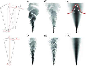


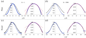


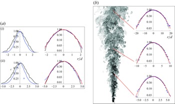


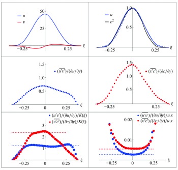


 Open access