





1. Introduction
The transfer of energy from large to small scales is a defining feature of three-dimensional turbulent flows, e.g. Alexakis & Biferale (Reference Alexakis and Biferale2018). However, geometric constraints or strongly anisotropic forcings can result in some of the injected energy being transferred to scales that are larger than the forcing scale, leading to the emergence of coherent structures in coexistence with small-scale turbulence, also known as turbulent superstructures. Examples of these structures can be found in wall-bounded turbulence (Kim & Adrian Reference Kim and Adrian1999; Guala, Hommema & Adrian Reference Guala, Hommema and Adrian2006; Hutchins & Marusic Reference Hutchins and Marusic2007), Rayleigh–Bénard convection (Hartlep, Tilgner & Busse Reference Hartlep, Tilgner and Busse2003; Parodi et al. Reference Parodi, von Hardenberg, Passoni, Provenzale and Spiegel2004; Emran & Schumacher Reference Emran and Schumacher2015; Pandey, Scheel & Schumacher Reference Pandey, Scheel and Schumacher2018; Stevens et al. Reference Stevens, Blass, Zhu, Verzicco and Lohse2018; Green et al. Reference Green, Vlaykov, Mellado and Wilczek2020; Krug, Lohse & Stevens Reference Krug, Lohse and Stevens2020), turbulent Taylor–Couette flow (Huisman et al. Reference Huisman, Van Der Veen, Sun and Lohse2014; van der Veen et al. Reference van der Veen, Huisman, Dung, Tang, Sun and Lohse2016) and turbulent Kolmogorov flow (Sarris et al. Reference Sarris, Jeanmart, Carati and Winckelmans2007; Lalescu & Wilczek Reference Lalescu and Wilczek2021) to mention a few. In some of these examples, the observed superstructures seem to be reminiscent of the structures arising from instabilities at low Reynolds numbers but persist far away from the onset of turbulence. Turbulent Kolmogorov flow is a prototypical example of a flow featuring the emergence of large-scale flow structures. The investigation of Kolmogorov flow has a long tradition in the field. Kolmogorov proposed the original problem as a two-dimensional flow to study the transition to turbulence in an analytically accessible setting (Arnold & Meshalkin Reference Arnold and Meshalkin1960). The stability of the two-dimensional Kolmogorov flow was investigated by Meshalkin & Sinai (Reference Meshalkin and Sinai1961), Thess (Reference Thess1992), Okamoto & Shōji (Reference Okamoto and Shōji1993), Iudovich (Reference Iudovich1965), Okamoto (Reference Okamoto1998) and more recently by Chatterjee & Verma (Reference Chatterjee and Verma2020) among others. The authors of these works discuss how a laminar solution parallel to the shear force loses stability, leading to the formation of vortex pairs whose size is comparable to the size of the bounding domain. Studies of this flow have not been restricted to addressing the stability of its laminar solution; they have also been concerned with the complex spatio-temporal dynamics it may exhibit. Chandler & Kerswell (Reference Chandler and Kerswell2013), for instance, demonstrated that the evolution of a specific Kolmogorov flow can be interpreted as the system transiently visiting a sequence of unstable invariant solutions of the Navier–Stokes equations. This approach has been extended to describe localised chaotic attractors in spatially extended Kolmogorov flows (Lucas & Kerswell Reference Lucas and Kerswell2014). Dallas, Seshasayanan & Fauve (Reference Dallas, Seshasayanan and Fauve2020) reported non-periodic switching of different turbulent states in the form of flow reversals by measuring the amplitude of the largest Fourier mode available. These recent examples demonstrate that the study of these flows retains its relevance and remains a reliable testing ground for investigating the complexity of turbulence through a dynamical systems framework. In recent years, interest has grown in the study of the three-dimensional flow, which exhibits further complexity. Subcritical transition into turbulence, large-scale intermittency, as well as large-scale vortices, have been observed (Borue & Orszag Reference Borue and Orszag1996; Sarris et al. Reference Sarris, Jeanmart, Carati and Winckelmans2007; van Veen & Goto Reference van Veen and Goto2016; Lalescu & Wilczek Reference Lalescu and Wilczek2021).
Here, we study the three-dimensional flow with aspect ratio $\alpha = L_y/L_x = 1/3$
in the turbulent regime far beyond the onset of instability of the laminar solution (
$\alpha = L_y/L_x = 1/3$
in the turbulent regime far beyond the onset of instability of the laminar solution ( ${\textit{Re}}\sim 10^2 {\textit{Re}}_c$
, where
${\textit{Re}}\sim 10^2 {\textit{Re}}_c$
, where $ {\textit{Re}}_c$
is the Reynolds number at which instability occurs). A numerical study of this Kolmogorov flow has been conducted by Lalescu & Wilczek (Reference Lalescu and Wilczek2021), where the authors reported different turbulent states with different numbers of large-scale vortex pairs. Moreover, the authors reported a permanent dynamics in the form of switching between the number of large-scale vortex pairs. Even though a comprehensive characterisation of a turbulent flow involves a vast number of degrees of freedom, in this work, we conjecture that the turbulent superstructures in the Kolmogorov flow can be fairly described by a comparably lower number of degrees of freedom. Araki, Bos & Goto (Reference Araki, Bos and Goto2023) recently developed a phenomenological reduced-order model to relate periodic behaviour at low
$ {\textit{Re}}_c$
is the Reynolds number at which instability occurs). A numerical study of this Kolmogorov flow has been conducted by Lalescu & Wilczek (Reference Lalescu and Wilczek2021), where the authors reported different turbulent states with different numbers of large-scale vortex pairs. Moreover, the authors reported a permanent dynamics in the form of switching between the number of large-scale vortex pairs. Even though a comprehensive characterisation of a turbulent flow involves a vast number of degrees of freedom, in this work, we conjecture that the turbulent superstructures in the Kolmogorov flow can be fairly described by a comparably lower number of degrees of freedom. Araki, Bos & Goto (Reference Araki, Bos and Goto2023) recently developed a phenomenological reduced-order model to relate periodic behaviour at low $ Re$
with quasiperiodic orbits at high
$ Re$
with quasiperiodic orbits at high $ Re$
in a Taylor–Green flow, closely related to Kolmogorov flow. In this manuscript, we will benefit from the fact that, in Kolmogorov flow, instabilities that give rise to large-scale structures at low
$ Re$
in a Taylor–Green flow, closely related to Kolmogorov flow. In this manuscript, we will benefit from the fact that, in Kolmogorov flow, instabilities that give rise to large-scale structures at low $ Re$
are captured by a discrete set of degrees of freedom. More generally speaking, when a stable fixed point in a multi-dimensional dynamical system loses stability, the asymptotic evolution of perturbations of this equilibrium evolves on a lower-dimensional manifold, known as the centre manifold (Carr Reference Carr1981; Elphick et al. Reference Elphick, Tirapegui, Brachet, Coullet and Iooss1987). A change of variables relates the original variables to the lower-dimensional ones. However, far away from the onset of these structures, particularly in the turbulent regime, the validity of this analytical description is lost. Despite this, the striking similarity between the structures observed close to the onset of instability and the ones observed in coexistence with the small-scale turbulent motions suggests that a similar set of equations may still describe the dynamics of these structures. A typical approach to isolate the large-scale dynamics from the turbulent fluctuations is to introduce an averaging procedure in the Navier–Stokes equation (Germano Reference Germano1992; Pope Reference Pope2000). However, the resulting equation for the averaged velocity field contains an additional unclosed stress term that depends on the statistics of the velocity fluctuations. This extra term encodes the interaction between the large-scale structures and the small-scale fluctuations, representing a significant modelling challenge. Motivated by the dynamical behaviour of the large scales in the three-dimensional Kolmogorov flow, we characterise the meandering of the system through different numbers of vortex pairs by a set of two complex amplitudes. By spatially averaging the Navier–Stokes equation of the Kolmogorov flow over the direction orthogonal to the forcing plane, we argue how the resulting equation for the averaged velocity field can be regarded as a stochastic equation for the large scales. By characterising the statistics of these two complex amplitudes, we construct a set of stochastic amplitude equations for the complex amplitudes. The statistical properties of this set of equations reproduce, up to a fair agreement, the dynamics of the data of the amplitudes gathered from the three-dimensional Kolmogorov flow.
$ Re$
are captured by a discrete set of degrees of freedom. More generally speaking, when a stable fixed point in a multi-dimensional dynamical system loses stability, the asymptotic evolution of perturbations of this equilibrium evolves on a lower-dimensional manifold, known as the centre manifold (Carr Reference Carr1981; Elphick et al. Reference Elphick, Tirapegui, Brachet, Coullet and Iooss1987). A change of variables relates the original variables to the lower-dimensional ones. However, far away from the onset of these structures, particularly in the turbulent regime, the validity of this analytical description is lost. Despite this, the striking similarity between the structures observed close to the onset of instability and the ones observed in coexistence with the small-scale turbulent motions suggests that a similar set of equations may still describe the dynamics of these structures. A typical approach to isolate the large-scale dynamics from the turbulent fluctuations is to introduce an averaging procedure in the Navier–Stokes equation (Germano Reference Germano1992; Pope Reference Pope2000). However, the resulting equation for the averaged velocity field contains an additional unclosed stress term that depends on the statistics of the velocity fluctuations. This extra term encodes the interaction between the large-scale structures and the small-scale fluctuations, representing a significant modelling challenge. Motivated by the dynamical behaviour of the large scales in the three-dimensional Kolmogorov flow, we characterise the meandering of the system through different numbers of vortex pairs by a set of two complex amplitudes. By spatially averaging the Navier–Stokes equation of the Kolmogorov flow over the direction orthogonal to the forcing plane, we argue how the resulting equation for the averaged velocity field can be regarded as a stochastic equation for the large scales. By characterising the statistics of these two complex amplitudes, we construct a set of stochastic amplitude equations for the complex amplitudes. The statistical properties of this set of equations reproduce, up to a fair agreement, the dynamics of the data of the amplitudes gathered from the three-dimensional Kolmogorov flow.
2. Three-dimensional Kolmogorov flow at low Reynolds number
We consider a Kolmogorov flow on a periodic domain of dimensions $6\pi \times 2\pi \times 2\pi$
. The governing equation is the incompressible Navier–Stokes equation
$6\pi \times 2\pi \times 2\pi$
. The governing equation is the incompressible Navier–Stokes equation
 \begin{align} \partial _t \boldsymbol u + \boldsymbol{u} {\cdot }\boldsymbol{\nabla }\boldsymbol{u} &= - \boldsymbol{\nabla }p + \nu {\nabla} ^2 \boldsymbol u - \bar {\mu } \bar {\boldsymbol u}+ f \sin \left ( k_f y \right )\boldsymbol e_x ,\end{align}
 \begin{align} \boldsymbol{\nabla \boldsymbol{\cdot }u} &= 0. \end{align}
Here, $\boldsymbol u$
is the three-dimensional velocity field,
$\boldsymbol u$
is the three-dimensional velocity field, $p$
is the (kinematic) pressure and
$p$
is the (kinematic) pressure and $\nu$
is the kinematic viscosity. The flow is damped by a large-scale drag with damping parameter
$\nu$
is the kinematic viscosity. The flow is damped by a large-scale drag with damping parameter $\bar {\mu }$
where (Lalescu & Wilczek Reference Lalescu and Wilczek2021)
$\bar {\mu }$
where (Lalescu & Wilczek Reference Lalescu and Wilczek2021)
 \begin{equation} \bar {\boldsymbol u} = \sum _{k \lt k_f} \hat {\boldsymbol u }(\boldsymbol k) \mathrm{e}^{\mathrm{i}\boldsymbol k \boldsymbol{\cdot }\boldsymbol x} \end{equation}
only contains modes with wavenumbers smaller than the forcing wavenumber $k_f$
. Lalescu & Wilczek (Reference Lalescu and Wilczek2021) showed that the introduction of a drag term that only acts on the large scales could modify the number of vortex pairs. The Kolmogorov flow is driven by forcing with amplitude
$k_f$
. Lalescu & Wilczek (Reference Lalescu and Wilczek2021) showed that the introduction of a drag term that only acts on the large scales could modify the number of vortex pairs. The Kolmogorov flow is driven by forcing with amplitude $f$
, which is constant in time and varies sinusoidally in a spanwise direction with wavenumber
$f$
, which is constant in time and varies sinusoidally in a spanwise direction with wavenumber $k_f$
. We non-dimensionalise the equations using
$k_f$
. We non-dimensionalise the equations using $L = 2\pi / k_f$
and
$L = 2\pi / k_f$
and $T = (L/f)^{1/2}$
as spatial and temporal scales, respectively. We define the forcing-based Reynolds number
$T = (L/f)^{1/2}$
as spatial and temporal scales, respectively. We define the forcing-based Reynolds number ${\textit{Re}}= UL / \nu = (2 \pi / k_f)^{3/2} f^{1/2}/ \nu$
, the non-dimensional large-scale drag coefficient
${\textit{Re}}= UL / \nu = (2 \pi / k_f)^{3/2} f^{1/2}/ \nu$
, the non-dimensional large-scale drag coefficient $\mu = T \bar {\mu }$
and the aspect ratio
$\mu = T \bar {\mu }$
and the aspect ratio $L_x/L_y = \alpha = 1/3$
. We keep the forcing amplitude fixed at
$L_x/L_y = \alpha = 1/3$
. We keep the forcing amplitude fixed at $f = 1/2$
and the forcing wavenumber at
$f = 1/2$
and the forcing wavenumber at $k_f = 1$
. By rescaling space as
$k_f = 1$
. By rescaling space as $\boldsymbol x = L \boldsymbol x^\prime$
, time as
$\boldsymbol x = L \boldsymbol x^\prime$
, time as $t = T t^\prime$
and dropping the primes we obtain
$t = T t^\prime$
and dropping the primes we obtain
 \begin{equation} \partial _t \boldsymbol u + \boldsymbol{u \boldsymbol{\cdot }\boldsymbol{\nabla }u} = - \boldsymbol{\nabla } p + \frac {1}{\textit{Re}} {\nabla} ^2 \boldsymbol u - \mu \bar {\boldsymbol u}+ \sin \left ( 2 \pi y\right ) \, \boldsymbol e_x . \end{equation}
For every value of $ Re$
and
$ Re$
and $\mu$
there exists a laminar solution given by
$\mu$
there exists a laminar solution given by $\boldsymbol u_{\mathrm{L}} = ({\textit{Re}}/{4\pi ^2}) \sin (2\pi y) \boldsymbol e_x,$
and homogeneous pressure
$\boldsymbol u_{\mathrm{L}} = ({\textit{Re}}/{4\pi ^2}) \sin (2\pi y) \boldsymbol e_x,$
and homogeneous pressure $p = p_0$
. The stability of this laminar solution has been characterised several times, e.g. by Meshalkin & Sinai (Reference Meshalkin and Sinai1961), Thess (Reference Thess1992) and Chatterjee & Verma (Reference Chatterjee and Verma2020), to mention a few. We extend the aforementioned linear stability analysis to include the large-scale drag. The Kolmogorov flow with a drag acting on all scales has already been considered by Thess (Reference Thess1992), who showed that the drag shifts the critical Reynolds number at which the laminar solution becomes unstable. To study perturbations to the laminar solution it is convenient to note that, since the laminar solution of (2.3) only depends on the
$p = p_0$
. The stability of this laminar solution has been characterised several times, e.g. by Meshalkin & Sinai (Reference Meshalkin and Sinai1961), Thess (Reference Thess1992) and Chatterjee & Verma (Reference Chatterjee and Verma2020), to mention a few. We extend the aforementioned linear stability analysis to include the large-scale drag. The Kolmogorov flow with a drag acting on all scales has already been considered by Thess (Reference Thess1992), who showed that the drag shifts the critical Reynolds number at which the laminar solution becomes unstable. To study perturbations to the laminar solution it is convenient to note that, since the laminar solution of (2.3) only depends on the $y$
-coordinate, the most unstable perturbations to such a flows are independent of the
$y$
-coordinate, the most unstable perturbations to such a flows are independent of the $z$
-coordinate, a result known as Squire’s theorem (Squire Reference Squire1933). We determine the stability of the laminar solution by studying the linear evolution of a streamfunction
$z$
-coordinate, a result known as Squire’s theorem (Squire Reference Squire1933). We determine the stability of the laminar solution by studying the linear evolution of a streamfunction $\psi (x,y,t)$
, from which the velocity is determined via
$\psi (x,y,t)$
, from which the velocity is determined via $\boldsymbol u(x,y,t) = \boldsymbol u_{\mathrm{L}}(y) + \boldsymbol{\nabla }\times (\psi (x,y,t) \boldsymbol e_z)$
. By taking the curl of (2.3), we obtain the following equation for the streamfunction:
$\boldsymbol u(x,y,t) = \boldsymbol u_{\mathrm{L}}(y) + \boldsymbol{\nabla }\times (\psi (x,y,t) \boldsymbol e_z)$
. By taking the curl of (2.3), we obtain the following equation for the streamfunction:
 \begin{align} \partial _t {\nabla} ^2 \psi &= \underbrace {\left (\frac {1}{\textit{Re}} {\nabla} ^4 -{\textit{Re}}\sin {( 2\pi y )} \left (1 + \frac {1}{4\pi ^2}{\nabla} ^2 \right )\partial _x \right ) \psi - \mu {\nabla} ^2 \bar {\psi }}_{\mathcal{L}\left (\mu , \boldsymbol{Re}; \psi \right )}\notag\\&\quad -\underbrace { \left ( \partial _y \psi \partial _x - \partial _x \psi \partial _y \right ) {\nabla} ^2 \psi }_{\mathcal{N}(\psi )} ,\end{align}
where we have used $\omega _z = (\boldsymbol{\nabla }\times \boldsymbol{u}) \boldsymbol{\cdot }\boldsymbol{e}_z = -(Re/2 \pi) \cos({2 \pi y})- {\nabla} ^2 \psi$
. We study perturbations of the form
$\omega _z = (\boldsymbol{\nabla }\times \boldsymbol{u}) \boldsymbol{\cdot }\boldsymbol{e}_z = -(Re/2 \pi) \cos({2 \pi y})- {\nabla} ^2 \psi$
. We study perturbations of the form
 \begin{equation} \psi _n(x,y,t) = \hat {\psi }_n(y) \mathrm{e}^{2\pi \mathrm{i} \alpha x + \lambda _n(\boldsymbol{Re} , \mu ) t} \text{,} \end{equation}
with $n \in \mathbb{Z}$
. Each
$n \in \mathbb{Z}$
. Each $ \psi _n(x,y,t)$
corresponds to an eigenvector of the operator
$ \psi _n(x,y,t)$
corresponds to an eigenvector of the operator $\mathcal{L}(\mu , {\textit{Re}}; \psi )$
. A mode
$\mathcal{L}(\mu , {\textit{Re}}; \psi )$
. A mode $\psi _n$
becomes unstable when the real part of
$\psi _n$
becomes unstable when the real part of $\lambda _n( Re, \mu )$
crosses
$\lambda _n( Re, \mu )$
crosses $0$
from below. For the aspect ratio (
$0$
from below. For the aspect ratio ( $\alpha = 1/3$
) we are considering, only the modes
$\alpha = 1/3$
) we are considering, only the modes $\psi _1$
and
$\psi _1$
and $\psi _2$
can become unstable, namely, for every value of
$\psi _2$
can become unstable, namely, for every value of $\mu$
there exist
$\mu$
there exist $ {\textit{Re}}_1(\mu )$
and
$ {\textit{Re}}_1(\mu )$
and $ {\textit{Re}}_2(\mu )$
such that
$ {\textit{Re}}_2(\mu )$
such that $\mathrm{\textit{Re}} \left \{\lambda _1( {\textit{Re}}_1(\mu ), \mu )\right \} =\mathrm{\textit{Re}} \left \{\lambda _1( {\textit{Re}}_2(\mu ), \mu )\right \}=0$
. When
$\mathrm{\textit{Re}} \left \{\lambda _1( {\textit{Re}}_1(\mu ), \mu )\right \} =\mathrm{\textit{Re}} \left \{\lambda _1( {\textit{Re}}_2(\mu ), \mu )\right \}=0$
. When $\psi _1$
becomes unstable for sufficiently high
$\psi _1$
becomes unstable for sufficiently high $ Re$
, a new state with a single vortex pair emerges as a secondary flow. On the other hand, when
$ Re$
, a new state with a single vortex pair emerges as a secondary flow. On the other hand, when $\psi _2$
becomes unstable, a state with two vortex pairs emerges instead. The linear stability analysis does not tell us whether these new states are stable solutions of the Navier–Stokes equations (2.3), we will determine the stability of these states using direct numerical simulations (DNS) and a weakly nonlinear analysis. In the frictionless case, perturbations with the smallest streamwise wavenumber are the most unstable ones (Meshalkin & Sinai Reference Meshalkin and Sinai1961), namely
$\psi _2$
becomes unstable, a state with two vortex pairs emerges instead. The linear stability analysis does not tell us whether these new states are stable solutions of the Navier–Stokes equations (2.3), we will determine the stability of these states using direct numerical simulations (DNS) and a weakly nonlinear analysis. In the frictionless case, perturbations with the smallest streamwise wavenumber are the most unstable ones (Meshalkin & Sinai Reference Meshalkin and Sinai1961), namely $ {\textit{Re}}_1(0)\lt {\textit{Re}}_2(0)$
, therefore the one-vortex-pair configuration is preferred at low
$ {\textit{Re}}_1(0)\lt {\textit{Re}}_2(0)$
, therefore the one-vortex-pair configuration is preferred at low $ Re$
. However, for
$ Re$
. However, for $\mu \gt \mu _c \approx 0.90$
, we have
$\mu \gt \mu _c \approx 0.90$
, we have $ {\textit{Re}}_2(\mu )\lt {\textit{Re}}_1(\mu )$
, and the two-vortex-pair configuration is preferred. At
$ {\textit{Re}}_2(\mu )\lt {\textit{Re}}_1(\mu )$
, and the two-vortex-pair configuration is preferred. At $\mu =\mu _c$
we have
$\mu =\mu _c$
we have
 \begin{align} {\textit{Re}}_2(\mu _c) = {\textit{Re}}_1(\mu _c) = {\textit{Re}}_c ,\end{align}
which means that both states can emerge when ${\textit{Re}}\gt {\textit{Re}}_c$
. Analytical expressions for
${\textit{Re}}\gt {\textit{Re}}_c$
. Analytical expressions for $\psi _1(x,y;\mu )$
and
$\psi _1(x,y;\mu )$
and $\psi _2(x,y;\mu )$
are approximately given by
$\psi _2(x,y;\mu )$
are approximately given by
 \begin{align} \psi _1(x,y;\mu ) &\approx \left ( 2 \mathrm{i}\sin {(2\pi y)} + \frac {16 \pi ^3\left (1 + \alpha ^2 \right )^2}{\alpha {\textit{Re}}_{1}^2(\mu )\left ( 1 - \alpha ^2 \right )} \right ) \mathrm{e}^{2 \pi \mathrm{i}\alpha (x -x_1) } , \end{align}
 \begin{align} \psi _2(x,y;\mu ) &\approx \left ( 2 \mathrm{i}\sin {(2\pi y)} + \frac {8 \pi ^3\left (1 + 4\alpha ^2 \right )^2}{\alpha {\textit{Re}}_{2}^2(\mu )\left ( 1 - 4\alpha ^2 \right )} \right ) \mathrm{e}^{4 \pi \mathrm{i}\alpha (x -x_2)} , \end{align}
(a) Regime map of the three-dimensional Kolmogorov flow at low Reynolds numbers, along with visualisations of the possible states. The blue curve with squares ( $ {\textit{Re}}_1^*(\mu )$
) corresponds to the lower stability threshold of the solution with one vortex pair, while the orange curve with squares (
$ {\textit{Re}}_1^*(\mu )$
) corresponds to the lower stability threshold of the solution with one vortex pair, while the orange curve with squares ( $ {\textit{Re}}_2^*(\mu )$
) corresponds to the lower stability threshold of the solution with two vortex pairs. Note that for
$ {\textit{Re}}_2^*(\mu )$
) corresponds to the lower stability threshold of the solution with two vortex pairs. Note that for $\mu \lt \mu _c \approx 0.90$
,
$\mu \lt \mu _c \approx 0.90$
, $ {\textit{Re}}_1^*(\mu )$
coincides with
$ {\textit{Re}}_1^*(\mu )$
coincides with $ {\textit{Re}}_1(\mu )$
plotted in a dotted blue curve corresponding to the
$ {\textit{Re}}_1(\mu )$
plotted in a dotted blue curve corresponding to the $ Re$
value where the state with one-vortex-pair emerges in a supercritical bifurcation, while for
$ Re$
value where the state with one-vortex-pair emerges in a supercritical bifurcation, while for $\mu \gt \mu _c$
,
$\mu \gt \mu _c$
, $ {\textit{Re}}_2^*(\mu )$
coincides with
$ {\textit{Re}}_2^*(\mu )$
coincides with $ {\textit{Re}}_2(\mu )$
, plotted in a dotted orange curve. Vertical black lines correspond to the section where we show the corresponding bifurcation diagrams in figure 2. (b) Visual representation of the possible flow configuration. The vertical component of the vorticity
$ {\textit{Re}}_2(\mu )$
, plotted in a dotted orange curve. Vertical black lines correspond to the section where we show the corresponding bifurcation diagrams in figure 2. (b) Visual representation of the possible flow configuration. The vertical component of the vorticity $\omega _z$
is coded in the colour map superimposed by a visualisation of the velocity field.
$\omega _z$
is coded in the colour map superimposed by a visualisation of the velocity field.

Figure 1. Long description
The image contains two main sections. The left section features a line graph showing the regime map of the three-dimensional Kolmogorov flow at low Reynolds numbers. The x-axis represents the parameter mu, ranging from 0 to 2, and the y-axis represents the Reynolds number, ranging from 20 to 45. The graph includes two curves: a blue curve with squares indicating the lower stability threshold of the solution with one vortex pair, and an orange curve with squares indicating the lower stability threshold of the solution with two vortex pairs. The graph also highlights a bistable zone and regions of stable laminar flow and one vortex pair. The right section features visual representations of the possible flow configurations. The top image shows no vortex pairs, the middle image shows one vortex pair, and the bottom image shows two vortex pairs. Each image depicts the vertical component of the vorticity with a color map and a visualization of the velocity field. The visualizations illustrate the flow patterns and the emergence of coherent structures in the Kolmogorov flow.
where $x_1$
and
$x_1$
and $x_2$
characterise the position along the
$x_2$
characterise the position along the $x$
-axis of the emerging unstable solutions. The expressions are approximated in the sense that the number of Fourier modes in the
$x$
-axis of the emerging unstable solutions. The expressions are approximated in the sense that the number of Fourier modes in the $y$
-direction has been truncated, see Appendix B for a detailed derivation of these expressions along with the computation of
$y$
-direction has been truncated, see Appendix B for a detailed derivation of these expressions along with the computation of $\mu _c$
and
$\mu _c$
and $ {\textit{Re}}_c$
. Combining these results with DNS allows us to obtain a regime map of this system at a low Reynolds number, which we display in figure 1 along with snapshots of the possible flow configurations in this region of the parameter space
$ {\textit{Re}}_c$
. Combining these results with DNS allows us to obtain a regime map of this system at a low Reynolds number, which we display in figure 1 along with snapshots of the possible flow configurations in this region of the parameter space $( \mu ,{\textit{Re}})$
. We construct this regime map in the following way: we run two sets of simulations with different initial conditions, one starting in the one-vortex-pair configuration, and the other in the two-vortex-pair configuration. We determine the streamfunction
$( \mu ,{\textit{Re}})$
. We construct this regime map in the following way: we run two sets of simulations with different initial conditions, one starting in the one-vortex-pair configuration, and the other in the two-vortex-pair configuration. We determine the streamfunction $\psi (x,y)$
, project it onto
$\psi (x,y)$
, project it onto $\psi _1(x,y)$
and
$\psi _1(x,y)$
and $\psi _2(x,y)$
and define the following amplitudes:
$\psi _2(x,y)$
and define the following amplitudes:
 \begin{align} a_1 &= \frac {\int _{0}^{1} \int _{0}^{3} \psi _1(x,y)^* \psi (x,y) \mathrm{d}x \mathrm{d}y}{\int _{0}^{1} \int _{0}^{3}|\psi _1(x,y)|^2 \mathrm{d}x \mathrm{d}y} , \end{align}
 \begin{align} a_2 &= \frac {\int _{0}^{1} \int _{0}^{3} \psi _2(x,y)^* \psi (x,y) \mathrm{d}x \mathrm{d}y}{\int _{0}^{1} \int _{0}^{3}|\psi _2(x,y)|^2 \mathrm{d}x \mathrm{d}y} . \end{align}
(a) Bifurcation diagram of the flow at $\mu = 0.25$
. Solid lines represent stable states while dashed lines represent unstable states. At
$\mu = 0.25$
. Solid lines represent stable states while dashed lines represent unstable states. At $ {\textit{Re}}_1$
the flow undergoes a pitchfork bifurcation which gives rise to a configuration with one vortex pair. At
$ {\textit{Re}}_1$
the flow undergoes a pitchfork bifurcation which gives rise to a configuration with one vortex pair. At $ {\textit{Re}}_2$
the flow undergoes another pitchfork bifurcation which leads to a configuration with two vortex pairs, however, this state is unstable. At
$ {\textit{Re}}_2$
the flow undergoes another pitchfork bifurcation which leads to a configuration with two vortex pairs, however, this state is unstable. At $ {\textit{Re}}_2^*$
, there is a saddle-node bifurcation that gives rise to a mixed state where
$ {\textit{Re}}_2^*$
, there is a saddle-node bifurcation that gives rise to a mixed state where $a_1 \neq 0$
and
$a_1 \neq 0$
and $a_2 \neq 0$
. After this bifurcation, the two-vortex-pair configuration becomes stable while the mixed state remains unstable. For
$a_2 \neq 0$
. After this bifurcation, the two-vortex-pair configuration becomes stable while the mixed state remains unstable. For $ Re\gt {\textit{Re}}_2^*$
the flow exhibits either one or two vortex pairs depending on the initial condition. (b) Bifurcation diagram of the flow at
$ Re\gt {\textit{Re}}_2^*$
the flow exhibits either one or two vortex pairs depending on the initial condition. (b) Bifurcation diagram of the flow at $\mu = 1.5$
, the situation is analogous to the plot on the left-hand side, but now for
$\mu = 1.5$
, the situation is analogous to the plot on the left-hand side, but now for $ {\textit{Re}}_1 \lt{\textit{Re}}\lt {\textit{Re}}_1^*$
the one-vortex-pair configuration is unstable and a saddle-node bifurcation gives rise to an unstable mixed state at
$ {\textit{Re}}_1 \lt{\textit{Re}}\lt {\textit{Re}}_1^*$
the one-vortex-pair configuration is unstable and a saddle-node bifurcation gives rise to an unstable mixed state at $ {\textit{Re}}_1^*$
.
$ {\textit{Re}}_1^*$
.

Figure 2. Long description
The image contains two bifurcation diagrams side by side. The left diagram shows the flow at a specific condition, with solid lines representing stable states and dashed lines representing unstable states. At a Reynolds number of approximately 25, the flow undergoes a pitchfork bifurcation, leading to a configuration with one vortex pair. At a Reynolds number slightly below 30, another pitchfork bifurcation occurs, resulting in a configuration with two vortex pairs, which is unstable. At a Reynolds number of approximately 32, a saddle-node bifurcation gives rise to a mixed state where both configurations coexist, with the two-vortex-pair configuration becoming stable. The right diagram shows the flow at a different condition, where the one-vortex-pair configuration is unstable, and a saddle-node bifurcation gives rise to an unstable mixed state at a Reynolds number of approximately 40. The diagrams illustrate how different flow states emerge and stabilize at and values of the large-scale drag.
Since the modes $\psi _1(x,y)$
and
$\psi _1(x,y)$
and $\psi _2(x,y)$
are made from different Fourier modes, they are orthogonal to each other under this inner product, namely
$\psi _2(x,y)$
are made from different Fourier modes, they are orthogonal to each other under this inner product, namely $\int _{0}^{1} \int _{0}^{3} \psi _1(x,y)^* \psi _2(x,y) \mathrm{d}x \mathrm{d}y = 0$
. If
$\int _{0}^{1} \int _{0}^{3} \psi _1(x,y)^* \psi _2(x,y) \mathrm{d}x \mathrm{d}y = 0$
. If $|a_1|\neq 0$
and
$|a_1|\neq 0$
and $|a_2| = 0$
, we say that the flow is in the one-vortex-pair configuration, while if
$|a_2| = 0$
, we say that the flow is in the one-vortex-pair configuration, while if $|a_2|\neq 0$
and
$|a_2|\neq 0$
and $|a_1| = 0$
, the flow is in the two-vortex-pair configuration. In principle, mixed states where
$|a_1| = 0$
, the flow is in the two-vortex-pair configuration. In principle, mixed states where $|a_2|\neq 0$
and
$|a_2|\neq 0$
and $|a_1| \neq 0$
would also be possible; however, numerical simulations reveal that there are no such states that are stable. We then start each set of simulation at fixed value of
$|a_1| \neq 0$
would also be possible; however, numerical simulations reveal that there are no such states that are stable. We then start each set of simulation at fixed value of $\mu$
in a state with
$\mu$
in a state with $|a_1|\neq 0$
and
$|a_1|\neq 0$
and $|a_2| = 0$
(
$|a_2| = 0$
( $|a_2|\neq 0$
and
$|a_2|\neq 0$
and $|a_1| = 0$
), decrease
$|a_1| = 0$
), decrease $ Re$
and determine
$ Re$
and determine $ {\textit{Re}}_1^*(\mu )$
(
$ {\textit{Re}}_1^*(\mu )$
( $ {\textit{Re}}_2^*(\mu )$
) when
$ {\textit{Re}}_2^*(\mu )$
) when $|a_1| = 0$
(
$|a_1| = 0$
( $|a_2|\neq 0$
). We present these results in figure 1. We note that when
$|a_2|\neq 0$
). We present these results in figure 1. We note that when $\mu \lt \mu _c$
, the two-vortex-pair configuration becomes unstable at
$\mu \lt \mu _c$
, the two-vortex-pair configuration becomes unstable at $ {\textit{Re}}_2^*(\mu ) \gt {\textit{Re}}_2(\mu )$
, namely, at a higher Reynolds number than the one predicted by the linear theory, while for
$ {\textit{Re}}_2^*(\mu ) \gt {\textit{Re}}_2(\mu )$
, namely, at a higher Reynolds number than the one predicted by the linear theory, while for $\mu \gt \mu _c$
, the two curves coincide, namely
$\mu \gt \mu _c$
, the two curves coincide, namely $ {\textit{Re}}_2^*(\mu ) = {\textit{Re}}_2(\mu )$
. Analogously, for
$ {\textit{Re}}_2^*(\mu ) = {\textit{Re}}_2(\mu )$
. Analogously, for $\mu \gt \mu _c$
, we have
$\mu \gt \mu _c$
, we have $ {\textit{Re}}_1^*(\mu ) \gt {\textit{Re}}_1(\mu )$
instead, while
$ {\textit{Re}}_1^*(\mu ) \gt {\textit{Re}}_1(\mu )$
instead, while $ {\textit{Re}}_1^*(\mu ) = {\textit{Re}}_1(\mu )$
for
$ {\textit{Re}}_1^*(\mu ) = {\textit{Re}}_1(\mu )$
for $\mu \lt \mu _c$
. For
$\mu \lt \mu _c$
. For $ Re\gt {\textit{Re}}_1^*(\mu ), {\textit{Re}}_2^*(\mu )$
both states are equilibrium states of the flow. Whether the flow displays one or two vortex pairs depends on the initial conditions, and thus we label this region the bistable zone in figure 1. To clarify the type of bifurcations the flow undergoes when changing
$ Re\gt {\textit{Re}}_1^*(\mu ), {\textit{Re}}_2^*(\mu )$
both states are equilibrium states of the flow. Whether the flow displays one or two vortex pairs depends on the initial conditions, and thus we label this region the bistable zone in figure 1. To clarify the type of bifurcations the flow undergoes when changing $ Re$
, in figure 2 we show the bifurcation diagram at two values of
$ Re$
, in figure 2 we show the bifurcation diagram at two values of $\mu$
. On the left plot, we consider
$\mu$
. On the left plot, we consider $\mu = 0.25 \lt \mu _c$
. Solid lines represent stable equilibrium values of
$\mu = 0.25 \lt \mu _c$
. Solid lines represent stable equilibrium values of $|a_1|$
and
$|a_1|$
and $|a_2|$
, while the dashed ones represent unstable ones. In this region of the parameter space, we have
$|a_2|$
, while the dashed ones represent unstable ones. In this region of the parameter space, we have
 \begin{align} {\textit{Re}}_1 \lt {\textit{Re}}_2 \lt {\textit{Re}}_2^* . \end{align}
When ${\textit{Re}}\gt {\textit{Re}}_1$
, the configuration with one vortex pair is always a stable equilibrium; for
${\textit{Re}}\gt {\textit{Re}}_1$
, the configuration with one vortex pair is always a stable equilibrium; for $ {\textit{Re}} \in ( {\textit{Re}}_2, {\textit{Re}}_2^*)$
, the two-vortex-pair solution exists but is only an unstable equilibrium; At
$ {\textit{Re}} \in ( {\textit{Re}}_2, {\textit{Re}}_2^*)$
, the two-vortex-pair solution exists but is only an unstable equilibrium; At ${\textit{Re}}= {\textit{Re}}_2^*$
, the two-vortex-pair configuration becomes stable and an unstable mixed state, namely a state where
${\textit{Re}}= {\textit{Re}}_2^*$
, the two-vortex-pair configuration becomes stable and an unstable mixed state, namely a state where $|a_1|, |a_2| \neq 0$
emerges. In the right plot we consider
$|a_1|, |a_2| \neq 0$
emerges. In the right plot we consider $\mu = 1.5 \gt \mu _c$
, where we have
$\mu = 1.5 \gt \mu _c$
, where we have
 \begin{align} {\textit{Re}}_2 \lt {\textit{Re}}_1 \lt {\textit{Re}}_1^* . \end{align}
The situation is analogous to one we just described: For ${\textit{Re}}\gt {\textit{Re}}_2$
, the two-vortex-pair configuration is always a stable equilibrium; for
${\textit{Re}}\gt {\textit{Re}}_2$
, the two-vortex-pair configuration is always a stable equilibrium; for ${\textit{Re}}\in ( {\textit{Re}}_1, {\textit{Re}}_1^*)$
, the one-vortex-pair configuration is an unstable equilibrium; at
${\textit{Re}}\in ( {\textit{Re}}_1, {\textit{Re}}_1^*)$
, the one-vortex-pair configuration is an unstable equilibrium; at ${\textit{Re}}= {\textit{Re}}_1^*$
, the one-vortex-pair configuration becomes stable, and again, an unstable mixed state emerges.
${\textit{Re}}= {\textit{Re}}_1^*$
, the one-vortex-pair configuration becomes stable, and again, an unstable mixed state emerges.
The bifurcation diagrams were obtained in the following way: we start by finding the vorticity of the two equilibrium configurations for a given $ Re\gt {\textit{Re}}_1^*, Re^*_2$
. Let
$ Re\gt {\textit{Re}}_1^*, Re^*_2$
. Let $\omega _1( Re)$
and
$\omega _1( Re)$
and $\omega _2( Re)$
be these vorticity configurations. To find the unstable saddle point, namely the unstable mixed state, we conduct multiple simulations using
$\omega _2( Re)$
be these vorticity configurations. To find the unstable saddle point, namely the unstable mixed state, we conduct multiple simulations using
 \begin{align} \omega _z(x,y) = \alpha \omega _1( Re) + (1 -\alpha )\omega _2( Re) \quad \text{with}\quad \alpha \in [0,1] \end{align}
as an initial condition for the vorticity. We then solve the Navier–Stokes equation in the vorticity formulation and keep track of whether the flow converges back to $\omega _1( Re)$
or to
$\omega _1( Re)$
or to $\omega _2( Re)$
for each value of
$\omega _2( Re)$
for each value of $\alpha$
. This way, we identify a point in the separatrix between the two configurations in the
$\alpha$
. This way, we identify a point in the separatrix between the two configurations in the $(|a_1|, |a_2|)$
plane. We finally set an initial condition lying in the vicinity of the separatrix and track the trajectory
$(|a_1|, |a_2|)$
plane. We finally set an initial condition lying in the vicinity of the separatrix and track the trajectory $(a_1(t), a_2(t))$
. We identify the saddle point as the slowest point of this trajectory, i.e. the point where
$(a_1(t), a_2(t))$
. We identify the saddle point as the slowest point of this trajectory, i.e. the point where $\sqrt {(\mathrm{d}a_1/\mathrm{d}t )^2 + (\mathrm{d}a_2/\mathrm{d}t )^2}$
is minimised. We call this mixed state a saddle point because the trajectory
$\sqrt {(\mathrm{d}a_1/\mathrm{d}t )^2 + (\mathrm{d}a_2/\mathrm{d}t )^2}$
is minimised. We call this mixed state a saddle point because the trajectory $(a_1(t),a_2(t))$
approaches it, slows down and then is repelled so that
$(a_1(t),a_2(t))$
approaches it, slows down and then is repelled so that $(a_1(t),a_2(t))$
ends up in one of the stable vortex configurations.
$(a_1(t),a_2(t))$
ends up in one of the stable vortex configurations.
At $\mu = \mu _c$
the curves
$\mu = \mu _c$
the curves $ Re(\mu )$
and
$ Re(\mu )$
and $ {\textit{Re}}_2(\mu )$
intersect. At this point, both stable solutions emerge in supercritical bifurcations. We call the point
$ {\textit{Re}}_2(\mu )$
intersect. At this point, both stable solutions emerge in supercritical bifurcations. We call the point $(\mu _c, {\textit{Re}}_c)$
the onset of bistability, because the laminar solution becomes unstable simultaneously to
$(\mu _c, {\textit{Re}}_c)$
the onset of bistability, because the laminar solution becomes unstable simultaneously to $\psi _1$
and
$\psi _1$
and $\psi _2$
in a supercritical bifurcation. At this point we can study how the modes
$\psi _2$
in a supercritical bifurcation. At this point we can study how the modes $\psi _1$
and
$\psi _1$
and $\psi _2$
interact with each other by choosing
$\psi _2$
interact with each other by choosing $\mu = \mu _c + \varepsilon \mu _0$
and
$\mu = \mu _c + \varepsilon \mu _0$
and ${\textit{Re}}= {\textit{Re}}_{c}( 1 +\varepsilon r )$
, where
${\textit{Re}}= {\textit{Re}}_{c}( 1 +\varepsilon r )$
, where $\varepsilon \ll 1$
is a scaling parameter and
$\varepsilon \ll 1$
is a scaling parameter and $\mu _0$
and
$\mu _0$
and $r$
are arbitrary values of order
$r$
are arbitrary values of order $1$
. Under these conditions, we introduce the following ansatz into (2.4):
$1$
. Under these conditions, we introduce the following ansatz into (2.4):
 \begin{equation} \psi = \varepsilon ^{1/2} \left ( a_1(t)\psi _1 + a_2(t)\psi _2 + \mathrm{c.c.} \right ) + w(a_1, a_2) ,\end{equation}
where $a_1(t),a_2(t)$
are complex amplitudes of the two modes, c.c. stands for complex conjugate, and
$a_1(t),a_2(t)$
are complex amplitudes of the two modes, c.c. stands for complex conjugate, and $w(a_1, a_2)\sim \mathcal{O}(\varepsilon )$
is a nonlinear function of the amplitudes. In Appendix C, we employ normal form theory (Carr Reference Carr1981; Elphick et al. Reference Elphick, Tirapegui, Brachet, Coullet and Iooss1987; Haragus & Iooss Reference Haragus and Iooss2011) to derive a set of gradient equations describing the evolution of amplitudes
$w(a_1, a_2)\sim \mathcal{O}(\varepsilon )$
is a nonlinear function of the amplitudes. In Appendix C, we employ normal form theory (Carr Reference Carr1981; Elphick et al. Reference Elphick, Tirapegui, Brachet, Coullet and Iooss1987; Haragus & Iooss Reference Haragus and Iooss2011) to derive a set of gradient equations describing the evolution of amplitudes
 \begin{align} \frac {\mathrm{d} a_1}{\mathrm{d}t^*} &= \delta _1 a_1 - \gamma _1 |a_1|^ 2a_1 - \eta _1 |a_2|^ 2a_1 = - \eta _1 \frac {\partial \mathcal{F}}{\partial a_1^*} ,\end{align}
 \begin{align} \frac {\mathrm{d} a_2}{\mathrm{d}t^*} &= \delta _2 a_2 - \gamma _2 |a_2|^ 2a_2 - \eta _2 |a_1|^ 2a_2 = - \eta _2 \frac {\partial \mathcal{F}}{\partial a_2^*}\mathrm{.} \end{align}
Here, $t^* = \varepsilon t$
is a slow time. All the coefficients are real numbers implying that these two equations minimise a functional
$t^* = \varepsilon t$
is a slow time. All the coefficients are real numbers implying that these two equations minimise a functional $\mathcal{F}$
given by
$\mathcal{F}$
given by
 \begin{equation} \mathcal{F} = - \delta _1 |a_1|^2/\eta _1 - \delta _2 |a_2|^2/\eta _2 + \gamma _1 |a_1|^4/2\eta _1 + \gamma _2 |a_2|^4/2\eta _2 + |a_1|^2 |a_2|^2/2 ,\end{equation}
where $\delta _1 = \delta _1(\mu _0, r)$
and
$\delta _1 = \delta _1(\mu _0, r)$
and $\delta _2 = \delta _2(\mu _0, r)$
. Expressions for both functions, as well as expressions for
$\delta _2 = \delta _2(\mu _0, r)$
. Expressions for both functions, as well as expressions for $\gamma _1, \gamma _2,\eta _1$
and
$\gamma _1, \gamma _2,\eta _1$
and $\eta _2$
, as functions of
$\eta _2$
, as functions of $\mu _c$
and
$\mu _c$
and $ {\textit{Re}}_c$
can be found in Appendix C. Such amplitude equations can also be obtained purely by symmetry arguments. The Navier–Stokes equation (2.1a
) remains invariant under translations along the
$ {\textit{Re}}_c$
can be found in Appendix C. Such amplitude equations can also be obtained purely by symmetry arguments. The Navier–Stokes equation (2.1a
) remains invariant under translations along the $x$
-axis. This means that vortex pairs can arise at any position along this axis. By looking at the unstable modes in (2.7), it becomes clear that displacing the vortex pairs along the
$x$
-axis. This means that vortex pairs can arise at any position along this axis. By looking at the unstable modes in (2.7), it becomes clear that displacing the vortex pairs along the $x$
-axis is equivalent to a phase shift of the complex exponential. These additional phases can then be absorbed into
$x$
-axis is equivalent to a phase shift of the complex exponential. These additional phases can then be absorbed into $a_1$
and
$a_1$
and $a_2$
. This implies that their respective evolution equations must be phase invariant so that all positions along the
$a_2$
. This implies that their respective evolution equations must be phase invariant so that all positions along the $x$
-axis are equally accessible. The phase invariance demands that only terms like
$x$
-axis are equally accessible. The phase invariance demands that only terms like $|a_1|^n a_1$
,
$|a_1|^n a_1$
, $|a_2|^n a_2$
,
$|a_2|^n a_2$
, $|a_1|^m |a_2|^n a_1$
and
$|a_1|^m |a_2|^n a_1$
and $|a_1|^n |a_2|^m a_1$
can appear in the amplitude equations, which is consistent with our result. The symmetry approach provides a basic structure for the amplitude equation, but gives no information about the values of the coefficients. We find that all the coefficients in (2.13) are real and positive, which restricts the range of behaviours that such an equation can exhibit. To summarise the implications of (2.13):
$|a_1|^n |a_2|^m a_1$
can appear in the amplitude equations, which is consistent with our result. The symmetry approach provides a basic structure for the amplitude equation, but gives no information about the values of the coefficients. We find that all the coefficients in (2.13) are real and positive, which restricts the range of behaviours that such an equation can exhibit. To summarise the implications of (2.13):
-
(i) When $\delta _1 \lt 0$
and
$\delta _2 \lt 0$
, (2.13) have only a one stable equilibrium point: the origin
$(|a_1|, |a_2|) = (0,0)$
representing the laminar state with no vortex pairs.
$\delta _1 \lt 0$
and
$\delta _2 \lt 0$
, (2.13) have only a one stable equilibrium point: the origin
$(|a_1|, |a_2|) = (0,0)$
representing the laminar state with no vortex pairs. -
(ii) When
$\delta _1$
becomes positive, the equilibrium lying on the
$|a_1|$
-axis emerges in a supercritical bifurcation, namely at
$(|a_1|,|a_2|) =(\sqrt {({\delta _1}/{\gamma _1})}, 0)$
representing the one-vortex-pair configuration. This emerging equilibrium is stable if
$( {\gamma _1}/{\eta _2}) \lt ( {\delta _1}/{\delta _2})$
or if
$\delta _2 \lt 0$
, and unstable otherwise. -
(iii) When
$\delta _2$
becomes positive, the equilibrium lying on the
$|a_2|$
-axis emerges in a supercritical bifurcation, namely at
$(|a_1|,|a_2|) = (0 ,\sqrt {( {\delta _2}/{\gamma _2})})$
representing the two-vortex-pair configuration. This emerging equilibrium is stable if
$({\delta _1}/{\delta _2}) \lt ( {\eta _1}/{\gamma _2})$
or if
$\delta _1 \lt 0$
, and unstable otherwise. -
(iv) When
$( {\gamma _1}/{\eta _2}) \lt ({\delta _1}/{\delta _2}) \lt ({\eta _1}/{\gamma _2})$
, there is an additional equilibrium point at
$( {\delta _2 \eta _1 - \delta _1 \eta _2})/({\eta _1 \eta _2 - \gamma _1 \gamma _2}), ({\delta _1 \eta _2 - \delta _2 \eta _1})/({\eta _1 \eta _2 - \gamma _1 \gamma _2})$
. This equilibrium corresponds to the mixed state and is a saddle point, i.e. it is an unstable equilibrium.


These analytical results are in agreement with the results we present in the regime map in figure 1 and the bifurcation diagrams in figure 2. The system evolves until reaching a stationary state corresponding to a minimum of the functional. Even though amplitude equations are, in principle, valid only around the point $(\mu _c, {\textit{Re}}_c)$
, our numerical study suggests that the structure of the equation remains valid further from this point and even when turbulence develops.
$(\mu _c, {\textit{Re}}_c)$
, our numerical study suggests that the structure of the equation remains valid further from this point and even when turbulence develops.
3. Connecting turbulent superstructures with the dynamics at low Reynolds number
For large Reynolds numbers, the flow is fully three-dimensional, and the results of the linear stability analysis are no longer valid. However, we observe persistent large-scale vortex pairs (Sarris et al. Reference Sarris, Jeanmart, Carati and Winckelmans2007; Lalescu & Wilczek Reference Lalescu and Wilczek2021). The large-scale vortices can be isolated using a spatial averaging procedure. Following Lalescu & Wilczek (Reference Lalescu and Wilczek2021), we define the vertically averaged velocity field as $\tilde {\boldsymbol u} = \int _0^{1} \boldsymbol u(x,y,z)\,\mathrm{d} z$
. We generate numerical data using the code TurTLE (Lalescu et al. Reference Lalescu, Bramas, Rampp and Wilczek2022) for two values of the Reynolds number (
$\tilde {\boldsymbol u} = \int _0^{1} \boldsymbol u(x,y,z)\,\mathrm{d} z$
. We generate numerical data using the code TurTLE (Lalescu et al. Reference Lalescu, Bramas, Rampp and Wilczek2022) for two values of the Reynolds number ( ${\textit{Re}}= 2851, 7184$
) and for a range of values of the non-dimensional friction coefficient (
${\textit{Re}}= 2851, 7184$
) and for a range of values of the non-dimensional friction coefficient ( $\mu \in [0.0, 1.24]$
), see Appendix A for details. To illustrate the different large-scale structures and how they coexist with a fully three-dimensional flow, we show snapshots of two different instants of a simulation of the three-dimensional Kolmogorov flow at
$\mu \in [0.0, 1.24]$
), see Appendix A for details. To illustrate the different large-scale structures and how they coexist with a fully three-dimensional flow, we show snapshots of two different instants of a simulation of the three-dimensional Kolmogorov flow at $\mu = 0.89$
and
$\mu = 0.89$
and ${\textit{Re}}= 2851$
in figure 3. In figure 3 (a), we show a volume rendering of the squared vorticity
${\textit{Re}}= 2851$
in figure 3. In figure 3 (a), we show a volume rendering of the squared vorticity $ \omega ^2 = (\boldsymbol {\nabla }\times \boldsymbol u)^2$
to illustrate the complexity of the three-dimensional flow. In figure 3 (b), we display the streamlines of the averaged horizontal velocity
$ \omega ^2 = (\boldsymbol {\nabla }\times \boldsymbol u)^2$
to illustrate the complexity of the three-dimensional flow. In figure 3 (b), we display the streamlines of the averaged horizontal velocity $\tilde {\boldsymbol u }_\bot = \tilde {u}_x \boldsymbol e_x + \tilde {u}_y \boldsymbol e_y$
superimposed with a colour map of the averaged
$\tilde {\boldsymbol u }_\bot = \tilde {u}_x \boldsymbol e_x + \tilde {u}_y \boldsymbol e_y$
superimposed with a colour map of the averaged $z$
-component of the vorticity
$z$
-component of the vorticity $\tilde {\omega }_z = \partial _x \tilde {u}_y - \partial _y \tilde {u}_x$
which makes large-scale vortex pairs readily visible. We observe two types of large-scale structures, one with a single pair of vortices and another displaying two vortex pairs. These states show a strong resemblance with the attractors that emerge after the laminar solution loses stability at a low Reynolds number, as discussed in § 2 (see figure 1). Such structures have also been reported in higher-resolution simulations with a Reynolds number up to
$\tilde {\omega }_z = \partial _x \tilde {u}_y - \partial _y \tilde {u}_x$
which makes large-scale vortex pairs readily visible. We observe two types of large-scale structures, one with a single pair of vortices and another displaying two vortex pairs. These states show a strong resemblance with the attractors that emerge after the laminar solution loses stability at a low Reynolds number, as discussed in § 2 (see figure 1). Such structures have also been reported in higher-resolution simulations with a Reynolds number up to ${\textit{Re}}= 18\,100$
(Lalescu & Wilczek Reference Lalescu and Wilczek2021). To quantify the resemblance between the dynamics at high and low Reynolds number we define the following velocity fields:
${\textit{Re}}= 18\,100$
(Lalescu & Wilczek Reference Lalescu and Wilczek2021). To quantify the resemblance between the dynamics at high and low Reynolds number we define the following velocity fields: $\boldsymbol u_0 = \sin (2 \pi y) \boldsymbol e_x$
,
$\boldsymbol u_0 = \sin (2 \pi y) \boldsymbol e_x$
, $\boldsymbol u_{1} = \boldsymbol{\nabla }\times (\psi _1 \boldsymbol e_z)$
and
$\boldsymbol u_{1} = \boldsymbol{\nabla }\times (\psi _1 \boldsymbol e_z)$
and $\boldsymbol u_{2} = \boldsymbol{\nabla }\times (\psi _2 \boldsymbol e_z)$
which correspond to velocity fields parallel to the forcing, the complex velocity generated by the streamfunction
$\boldsymbol u_{2} = \boldsymbol{\nabla }\times (\psi _2 \boldsymbol e_z)$
which correspond to velocity fields parallel to the forcing, the complex velocity generated by the streamfunction $\psi _1$
and the complex velocity field generated by
$\psi _1$
and the complex velocity field generated by $\psi _2$
, respectively. In addition, we introduce an inner product for two-component vector fields
$\psi _2$
, respectively. In addition, we introduce an inner product for two-component vector fields $\langle \boldsymbol F, \boldsymbol G\rangle = 1/3\int _0^{1} \int _0^{3} (F_x G_x^* + F_y G_y^* )\mathrm{d}x \, \mathrm{d}y$
. The velocity fields
$\langle \boldsymbol F, \boldsymbol G\rangle = 1/3\int _0^{1} \int _0^{3} (F_x G_x^* + F_y G_y^* )\mathrm{d}x \, \mathrm{d}y$
. The velocity fields $\boldsymbol u_0, \boldsymbol u_1$
, and
$\boldsymbol u_0, \boldsymbol u_1$
, and $\boldsymbol u_2$
are orthogonal to each other with respect to this inner product. We use these large-scale velocity fields to decompose the average velocity
$\boldsymbol u_2$
are orthogonal to each other with respect to this inner product. We use these large-scale velocity fields to decompose the average velocity
 \begin{align} \tilde {\boldsymbol u} = \underbrace {A_0(t)\boldsymbol u_0 + \left [A_1(t)\boldsymbol u_1+ A_2(t)\boldsymbol u_2 + \mathrm{c.c.}\right ]}_{\boldsymbol u_{\textit{TS}}(t,x,y)}\,+\,{\boldsymbol u}_{{R}}(t,x,y) + \tilde {u}_z(t,x,y) \boldsymbol e_z ,\end{align}
where $A_i(t) = \langle \boldsymbol u_i, \boldsymbol u \rangle / \langle \boldsymbol u_i, \boldsymbol u_i \rangle$
for
$A_i(t) = \langle \boldsymbol u_i, \boldsymbol u \rangle / \langle \boldsymbol u_i, \boldsymbol u_i \rangle$
for $i=0,1,2$
. We name
$i=0,1,2$
. We name $\boldsymbol u_{\textit{TS}}$
the component of the average velocity field that belongs to the subspace generated by
$\boldsymbol u_{\textit{TS}}$
the component of the average velocity field that belongs to the subspace generated by $\boldsymbol u_0, \boldsymbol u_1$
and
$\boldsymbol u_0, \boldsymbol u_1$
and $\boldsymbol u_2$
, where TS stands for turbulent superstructures. That means we effectively identify the vortices at low Reynolds numbers with the turbulent superstructures at high Reynolds numbers. By construction, we have that the remainder velocity field
$\boldsymbol u_2$
, where TS stands for turbulent superstructures. That means we effectively identify the vortices at low Reynolds numbers with the turbulent superstructures at high Reynolds numbers. By construction, we have that the remainder velocity field $\boldsymbol u_{{R}}$
is orthogonal to both
$\boldsymbol u_{{R}}$
is orthogonal to both $\boldsymbol u_{\textit{TS}}$
and
$\boldsymbol u_{\textit{TS}}$
and $\tilde {u}_z \boldsymbol e_z$
. We use the decomposition (3.1) to study the instantaneous two-dimensional energy decomposition, which is given by
$\tilde {u}_z \boldsymbol e_z$
. We use the decomposition (3.1) to study the instantaneous two-dimensional energy decomposition, which is given by
 \begin{equation} E_{2{D}}(t) = \frac {1}{3}\int _{0}^{1} \int _{0}^{3} \frac {1}{2}\left ( \boldsymbol u_{\textit{TS}}^2 + \boldsymbol u_{{R}}^2 + \tilde {u}_z^2\right ) \mathrm{d}x \, \mathrm{d}y = E_{\textit{TS}}(t) + E_{{R}}(t) + E_z(t) . \end{equation}
In figure 4 we display the time evolution of the instantaneous ratio between $E_{\textit{TS}}, E_{{R}}, E_z$
and
$E_{\textit{TS}}, E_{{R}}, E_z$
and $E_{{2D}}$
for the same simulation shown in figure 3. We observe that, on average, around
$E_{{2D}}$
for the same simulation shown in figure 3. We observe that, on average, around $76\,\%$
of the two-dimensional energy is contained within the large-scale velocity modes. We consider the total energy decomposition as well
$76\,\%$
of the two-dimensional energy is contained within the large-scale velocity modes. We consider the total energy decomposition as well
 \begin{equation} E_{3{D}}(t) = \frac {1}{3}\int _{0}^{1} \int _{0}^{1} \int _{0}^{3} \frac {1}{2}\left ( \tilde {\boldsymbol u}^2 + \boldsymbol u^{\prime 2}\right ) \mathrm{d}x\, \mathrm{d}y\,\mathrm{d}z = E_{2{D}}(t) + E^\prime (t), \end{equation}
where $\boldsymbol{u}^\prime = \boldsymbol{u} - \tilde{\boldsymbol{u}}$
. We find that energy in the turbulent superstructures makes up most of the two-dimensional energy for a wide range of
$\boldsymbol{u}^\prime = \boldsymbol{u} - \tilde{\boldsymbol{u}}$
. We find that energy in the turbulent superstructures makes up most of the two-dimensional energy for a wide range of $\mu$
and, therefore, a significant fraction of the total energy; we present these results in figure 5.
$\mu$
and, therefore, a significant fraction of the total energy; we present these results in figure 5.
(a) Volume rendering of the squared vorticity $\omega ^2$
at two different instants for the simulation at
$\omega ^2$
at two different instants for the simulation at ${\textit{Re}}= 2851$
and
${\textit{Re}}= 2851$
and $\mu = 0.89$
(see Appendix A). (b) Corresponding streamlines of the averaged horizontal velocity
$\mu = 0.89$
(see Appendix A). (b) Corresponding streamlines of the averaged horizontal velocity $\tilde {\boldsymbol u}_\bot (x,y)$
superimposed on the averaged
$\tilde {\boldsymbol u}_\bot (x,y)$
superimposed on the averaged $z$
-component of the vorticity to the volume renderings above.
$z$
-component of the vorticity to the volume renderings above.

Figure 3. Long description
The image contains two sets of visualizations related to turbulent Kolmogorov flow. The top row features volume renderings of the squared vorticity at two different time instants for a specific simulation. The color scale on the right indicates the intensity of the squared vorticity, ranging from 0 to 1. The bottom row displays the corresponding streamlines of the averaged horizontal velocity superimposed on the averaged z-component of the vorticity. The color scale on the right of the bottom row indicates the intensity of the z-component of the vorticity, ranging from −2.5 to 2.5. The streamlines illustrate the flow patterns and the vorticity component provides insights into the turbulent structures within the flow. The visualizations highlight the complex spatio-temporal dynamics and the emergence of large-scale flow structures in turbulent Kolmogorov flow.
Time evolution of the energy decomposition of the averaged two-dimensional flow for a simulation at ${\textit{Re}}= 2851$
and
${\textit{Re}}= 2851$
and $\mu = 0.89$
. Each time series represents the share of each term in (3.2) of the total two-dimensional energy
$\mu = 0.89$
. Each time series represents the share of each term in (3.2) of the total two-dimensional energy $E_{2{D}}$
. Here,
$E_{2{D}}$
. Here, $E_{\textit{TS}}$
is the energy contained in the turbulent superstructures,
$E_{\textit{TS}}$
is the energy contained in the turbulent superstructures, $E_{{R}}$
is the energy contained in the remaining modes of the averaged horizontal velocity
$E_{{R}}$
is the energy contained in the remaining modes of the averaged horizontal velocity $\tilde {\boldsymbol u}_\bot$
which are orthogonal to
$\tilde {\boldsymbol u}_\bot$
which are orthogonal to $\boldsymbol{u}_{\textit{TS}}$
and
$\boldsymbol{u}_{\textit{TS}}$
and $E_z$
is the energy contained in the averaged vertical velocity
$E_z$
is the energy contained in the averaged vertical velocity $u_z$
. The horizontal lines correspond to the time averages of the different fractions.
$u_z$
. The horizontal lines correspond to the time averages of the different fractions.

Figure 4. Long description
The line graph displays the time evolution of energy decomposition in a flow simulation. The x-axis represents time normalized by a time scale T, ranging from 0 to 1500. The y-axis represents the energy fractions normalized by the total two-dimensional energy E2D. Three data lines are present: a blue line representing the energy contained in turbulent superstructures (ETS/E2D), an orange line representing the energy contained in the remaining modes of the averaged horizontal velocity (ER/E2D), and a green line representing the energy contained in the averaged vertical velocity (Ez/E2D). The blue line fluctuates around a time average of 0.76, the orange line fluctuates around a time average of 0.19, and the green line fluctuates around a time average of 0.05.
Time-averaged energy ratios of turbulent superstructures. Shown are the fractions of energy contained in the large-scale modes relative to the total energy $E_{3D}$
and to the two-dimensional average
$E_{3D}$
and to the two-dimensional average $E_{2D}$
.
$E_{2D}$
.

Figure 5. Long description
The image contains two line graphs side by side, each representing the time-averaged energy ratios of turbulent superstructures at different Reynolds numbers. The left graph corresponds to a Reynolds number of 2851, while the right graph corresponds to a Reynolds number of 7184. Both graphs plot the fractions of energy contained in the large-scale modes relative to the total energy and to the two-dimensional average. The x-axis in both graphs represents the variable mu, ranging from 0 to 1.25. The y-axis represents the energy ratios, ranging from 0 to 1. In each graph, two data series are plotted: one with blue stars and another with orange circles. The blue stars represent the ratio of energy in turbulent superstructures to the three-dimensional total energy, while the orange circles represent the ratio of energy in turbulent superstructures to the two-dimensional average energy. In the left graph, the orange circles show an increasing trend as mu increases, starting around 0.6 and reaching approximately 0.8. The blue stars show a relatively stable trend around 0.4. In the right graph, the orange circles also show an increasing trend, starting around 0.6 and reaching approximately 0.85. The blue stars again show a relatively stable trend around 0.4. The graphs illustrate how the energy ratios vary with different values of mu and Reynolds numbers, highlighting the presence of turbulent superstructures in the flow.
(a) Time evolution of the amplitude $A_0(t)$
, with the best-fit linear regression from (3.4) superimposed for a simulation at
$A_0(t)$
, with the best-fit linear regression from (3.4) superimposed for a simulation at ${\textit{Re}}= 2851$
and
${\textit{Re}}= 2851$
and $\mu = 0.89$
. (b) The
$\mu = 0.89$
. (b) The $10T$
-averaged signal
$10T$
-averaged signal $\langle A_0(t) \rangle _{10T}$
compared with the averaged regression.
$\langle A_0(t) \rangle _{10T}$
compared with the averaged regression.

Figure 6. Long description
Two line graphs. The top graph shows the time evolution of the amplitude with the best-fit linear regression superimposed. The x-axis represents time normalized by T, ranging from 0 to 1500, and the y-axis represents the amplitude A0(t), ranging from 0.5 to 2.5. The orange line represents the best-fit linear regression equation 1.74 minus 6.74 times the square of the absolute value of A 1 minus 10.79 times the square of the absolute value of A2. The blue line represents the actual data points. The bottom graph shows the signal averaged over a time window of length 10T with the averaged regression. The x-axis represents time normalized by T, ranging from 0 to 1500, and the y-axis represents the T-averaged amplitude A0(t), ranging from 0.5 to 2.5. The orange line represents the averaged regression equation 1.74 minus the average of 6.74 times the square of the absolute value of A1 averaged over a time window of 10T plus 10.79 times the square of the absolute value of averaged over a time window of 10T. The blue line represents the actual averaged data points.
Time series of the evolution of the moduli of the complex amplitude $A_1(t)$
and
$A_1(t)$
and $A_2(t)$
for a simulation at
$A_2(t)$
for a simulation at ${\textit{Re}}= 2851$
and
${\textit{Re}}= 2851$
and $\mu = 0.89$
. The vertical lines correspond to the time stamps at where we extracted the visualisations in figure 3.
$\mu = 0.89$
. The vertical lines correspond to the time stamps at where we extracted the visualisations in figure 3.

Figure 7. Long description
The two line graph displays the evolution of the moduli of the complex amplitudes over time in a simulation. The x-axis represents time normalized by T, ranging from 0 to 750. The y-axis represents the moduli values, ranging from 0 to 0.4. Two data series are plotted: one in blue representing the modulus of the complex amplitude A1(t), and the other in orange representing the modulus of the complex amplitude A2(t). The graph shows fluctuations in both data series over time, with notable interactions and variations. Vertical dashed lines at specific time stamps indicate where visualizations were extracted for further analysis.
To simplify the problem even further, we conjecture that $A_0(t)$
is not an independent degree of freedom but instead is a function of the instantaneous values
$A_0(t)$
is not an independent degree of freedom but instead is a function of the instantaneous values $A_1(t)$
and
$A_1(t)$
and $A_2(t)$
. We base this assumption on the fact that, at low
$A_2(t)$
. We base this assumption on the fact that, at low $ Re$
, disturbances to the laminar solution are proportional to
$ Re$
, disturbances to the laminar solution are proportional to $|a_1|^2$
and
$|a_1|^2$
and $|a_2|^2$
, as shown in Appendix C. We propose an analogous decomposition
$|a_2|^2$
, as shown in Appendix C. We propose an analogous decomposition
 \begin{equation} A_0(t) = c_0 + c_1 |A_1(t)|^2 + c_2 |A_2(t)|^2 + \mathrm{h.o.t.} \end{equation}
Here, the set of coefficients $\{ c_i \}$
is determined using a linear regression. In figure 6, we keep track of the time evolution of the amplitude
$\{ c_i \}$
is determined using a linear regression. In figure 6, we keep track of the time evolution of the amplitude $A_0(t)$
, superimposed with the best linear regression. We find a good agreement between the linear regression and the instantaneous value of
$A_0(t)$
, superimposed with the best linear regression. We find a good agreement between the linear regression and the instantaneous value of $A_0(t)$
up to short-term fluctuations. This agreement becomes clearer after eliminating the fluctuations by averaging the data over a time window of length
$A_0(t)$
up to short-term fluctuations. This agreement becomes clearer after eliminating the fluctuations by averaging the data over a time window of length $10T$
$10T$
 \begin{equation} \langle A_0(t)\rangle _{10T} = \frac {1}{10T} \int _{-5T}^{5T} A_0(t - t^\prime )\mathrm{d}t^\prime .\end{equation}
The time-averaged data and linear regression results are displayed in figure 6(b). From these results, we conclude that the amplitude $A_0$
is not the independent degree of freedom but instead enslaved to the evolution of
$A_0$
is not the independent degree of freedom but instead enslaved to the evolution of $A_1$
and
$A_1$
and $A_2$
. We focus on the time evolution of these amplitudes; in figure 7, we show the temporal evolution of the moduli
$A_2$
. We focus on the time evolution of these amplitudes; in figure 7, we show the temporal evolution of the moduli $|A_1|$
and
$|A_1|$
and $|A_2|$
, which exhibit two distinct time scales. On the slowest time scale of the order of
$|A_2|$
, which exhibit two distinct time scales. On the slowest time scale of the order of $100T$
, there are time intervals where
$100T$
, there are time intervals where $|A_1| \gt |A_2| \sim 0$
and vice versa. The times
$|A_1| \gt |A_2| \sim 0$
and vice versa. The times $t_1$
and
$t_1$
and $t_2$
are the time stamps corresponding to the snapshots of the flow we display in figure 3. There is a correspondence between the number of large-scale vortices and the dominating amplitude. The system spends a finite time around one state before switching into the other, a phenomenon referred to as dynamical switching, which has already been observed by Lalescu & Wilczek (Reference Lalescu and Wilczek2021). We observe fast fluctuations around the equilibrium states on a shorter time scale than the switching scale. We proceed to characterise the different regions of the
$t_2$
are the time stamps corresponding to the snapshots of the flow we display in figure 3. There is a correspondence between the number of large-scale vortices and the dominating amplitude. The system spends a finite time around one state before switching into the other, a phenomenon referred to as dynamical switching, which has already been observed by Lalescu & Wilczek (Reference Lalescu and Wilczek2021). We observe fast fluctuations around the equilibrium states on a shorter time scale than the switching scale. We proceed to characterise the different regions of the $(A_1, A_2)$
space according to the number of large-scale vortices; for this, we take a sample of long time series of
$(A_1, A_2)$
space according to the number of large-scale vortices; for this, we take a sample of long time series of $A_1(t)$
and
$A_1(t)$
and $A_2(t)$
and use the classification algorithm KMeans (MacQueen Reference MacQueen1967) to partition the space into two disjoint regions
$A_2(t)$
and use the classification algorithm KMeans (MacQueen Reference MacQueen1967) to partition the space into two disjoint regions $\varOmega _1$
and
$\varOmega _1$
and $\varOmega _2$
. The result of the partition is displayed in figure 8: the upper row shows scatter plots of the real and imaginary parts of
$\varOmega _2$
. The result of the partition is displayed in figure 8: the upper row shows scatter plots of the real and imaginary parts of $A_1$
and
$A_1$
and $A_2$
, respectively. The blue points correspond to the sample points belonging to
$A_2$
, respectively. The blue points correspond to the sample points belonging to $\varOmega _1$
, which we identify as the instants where the flow is in a one-vortex-pair configuration, while the orange stars correspond to the samples belonging to
$\varOmega _1$
, which we identify as the instants where the flow is in a one-vortex-pair configuration, while the orange stars correspond to the samples belonging to $\varOmega _2$
, which we associate with the two-vortex-pair configuration. In the lower row of figure 8, we present histograms of the moduli
$\varOmega _2$
, which we associate with the two-vortex-pair configuration. In the lower row of figure 8, we present histograms of the moduli $|A_1|$
and
$|A_1|$
and $|A_2|$
, the blue bars correspond to the samples in
$|A_2|$
, the blue bars correspond to the samples in $\varOmega _1$
, while the orange ones to samples in
$\varOmega _1$
, while the orange ones to samples in $\varOmega _2$
. These histograms emphasise the switching between the dominant mode. Using conditional averages over these two sets, we can extract the modulus of equilibria around which the amplitudes oscillate, for
$\varOmega _2$
. These histograms emphasise the switching between the dominant mode. Using conditional averages over these two sets, we can extract the modulus of equilibria around which the amplitudes oscillate, for $\varOmega _1$
we find that
$\varOmega _1$
we find that $A_1^{\textit{mean}} = 0.31 \pm 0.04$
and for
$A_1^{\textit{mean}} = 0.31 \pm 0.04$
and for $\varOmega _2$
we find
$\varOmega _2$
we find $A_2^{\textit{mean}} = 0.14 \pm 0.05$
.
$A_2^{\textit{mean}} = 0.14 \pm 0.05$
.
(a) Partition of $(A_1,A_2)$
using the KMeans algorithm from the data of the simulation at
$(A_1,A_2)$
using the KMeans algorithm from the data of the simulation at ${\textit{Re}}= 2851$
and
${\textit{Re}}= 2851$
and $\mu = 0.89$
, we observe that the region
$\mu = 0.89$
, we observe that the region $\varOmega _1$
is characterised by
$\varOmega _1$
is characterised by $A_1$
oscillating around a ring of radius
$A_1$
oscillating around a ring of radius $A_1^{\textit{mean}}$
while
$A_1^{\textit{mean}}$
while $A_2$
oscillates around the origin of the complex plane. In the region
$A_2$
oscillates around the origin of the complex plane. In the region $\varOmega _2$
, we observe that
$\varOmega _2$
, we observe that $A_2$
oscillates around a ring of radius
$A_2$
oscillates around a ring of radius $A_2^{\textit{mean}}$
and it is
$A_2^{\textit{mean}}$
and it is $A_1$
that remains close to the origin. (b) Histograms of
$A_1$
that remains close to the origin. (b) Histograms of $|A_1|$
and
$|A_1|$
and $|A_2|$
conditioned on
$|A_2|$
conditioned on $\varOmega _1$
and
$\varOmega _1$
and $\varOmega _2$
.
$\varOmega _2$
.

Figure 8. Long description
The image contains two scatter plots and two histograms. The top row features two scatter plots. The left scatter plot shows data in blue points and orange stars. The x position of each data point corresponds the value of the real part of A1, while the y position corresponds to imaginary part of A1. Blue points correspond to instants where the flow is in the one-vortex configuration while the orange stars correspond to the instants when the flow is in the two-vortex configuration. The dashed circle marks A1mean, the average distance of the blue dots to the origin. The right scatter plot also displays data in blue points and orange stars. The x position of each data point corresponds now to the value of the real part of A2, while y position to its imaginary part. The dashed circle marks A2mean, the average distance of the orange stars to the origin. The bottom row contains two histograms. The left histogram shows the counts of the values of |A_1|, while the right one counts of |A_2|. The blue bars correspond to the data from the region \Sigma_1, meaning the flow is the one-vortex configuration, while the orange bars correspond to the data from the region \Sigma_2, namely, when the flow is in two-vortex configuration. The scatter plots and histograms illustrate the partitioning of data using the KMeans algorithm, highlighting regions where variables scatter around specific values.
The switching between states and the fluctuations resemble the dynamics of a stochastic process governed by a Langevin equation whose deterministic part corresponds to a double-well potential, such as that found in (2.14). Such analogies are not a novelty; for example, Benzi (Reference Benzi2005) argues how a background of turbulence can be regarded as a noise term on an effective equation for the large scales and uses this as a model to understand spontaneous flow reversals as a result of a noise-induced transition. An analogy with a low-dimensional stochastic model is also presented in Bouchet & Simonnet (Reference Bouchet and Simonnet2009) to model transitions between large-scale jets and box-size vortices on a stochastically forced two-dimensional Navier–Stokes equation. In the next section, we use this observation to construct a model for the amplitudes $A_1$
and
$A_1$
and $A_2$
.
$A_2$
.
4. Reduced-order model
4.1. Effective amplitude equations
We have shown that only two complex degrees of freedom can describe the turbulent superstructures fairly well. We observe three main qualitative features in the fully three-dimensional flow: first, the dynamics of $A_1(t)$
and
$A_1(t)$
and $A_2(t)$
exhibits two time scales. Second, on average, a significant fraction of the total two-dimensional energy is contained within the large-scale modes. Third, the dynamics of
$A_2(t)$
exhibits two time scales. Second, on average, a significant fraction of the total two-dimensional energy is contained within the large-scale modes. Third, the dynamics of $A_1(t)$
and
$A_1(t)$
and $A_2(t)$
resembles that of a bistable system. The bistable structure we characterised at a low Reynolds number remains in this regime. Considering the translation symmetry in the
$A_2(t)$
resembles that of a bistable system. The bistable structure we characterised at a low Reynolds number remains in this regime. Considering the translation symmetry in the $x$
-direction of the original Navier–Stokes equation (2.1a
), we conclude that the evolution equations for
$x$
-direction of the original Navier–Stokes equation (2.1a
), we conclude that the evolution equations for $A_1$
and
$A_1$
and $A_2$
must be phase invariant. Therefore, if they were the only relevant degrees of freedom, then their equations must be of the form
$A_2$
must be phase invariant. Therefore, if they were the only relevant degrees of freedom, then their equations must be of the form
 \begin{align} \frac {\mathrm{d} A_1}{\mathrm{d}t} &= \sum _{j,k=0}^{\infty } C_{j,k} |A_1|^{2j} |A_2|^{2k} A_1 ,\end{align}
 \begin{align} \frac {\mathrm{d} A_2}{\mathrm{d}t} &= \sum _{j, k =0}^{\infty } D_{j,k} |A_1|^{2j} |A_2|^{2k} A_2. \end{align}
Even allowing $C_{j,k}$
and
$C_{j,k}$
and $D_{j,k}$
to be complex, a system of equations like this cannot exhibit a complex dynamics like the one we observe when measuring these amplitudes on the numerical simulations. By separating these equations into modulus and phase, we find that the moduli evolve independently from the phases, rendering the system effectively a two-component system. Such a system can, at most, allow periodic orbits in the
$D_{j,k}$
to be complex, a system of equations like this cannot exhibit a complex dynamics like the one we observe when measuring these amplitudes on the numerical simulations. By separating these equations into modulus and phase, we find that the moduli evolve independently from the phases, rendering the system effectively a two-component system. Such a system can, at most, allow periodic orbits in the $(|A_1|, |A_2|)$
space. One way of inducing a complex permanent dynamics is to couple the evolution of the amplitudes with the small scales of the three-dimensional flow. Instead of introducing these degrees of freedom as additional amplitudes, we model the effect of the small scales in the form of explicit time-dependent functions in the reduced model. The following Langevin equations give the simplest of these models that can exhibit bistability:
$(|A_1|, |A_2|)$
space. One way of inducing a complex permanent dynamics is to couple the evolution of the amplitudes with the small scales of the three-dimensional flow. Instead of introducing these degrees of freedom as additional amplitudes, we model the effect of the small scales in the form of explicit time-dependent functions in the reduced model. The following Langevin equations give the simplest of these models that can exhibit bistability:
 \begin{align} \frac {\mathrm{d}A_1}{\mathrm{d}t} &= -\eta ^\prime _1 \frac {\partial F}{\partial A_{1}^*} + \sigma _1^\prime (t) ,\end{align}
 \begin{align} \frac {\mathrm{d}A_2}{\mathrm{d}t} &= -\eta ^\prime _2\frac {\partial F}{\partial A_{2}^*} + \sigma ^\prime _2(t) ,\end{align}
where $F$
is a functional analogous to
$F$
is a functional analogous to $\mathcal{F}$
in § 2
$\mathcal{F}$
in § 2
 \begin{equation} F = - \delta _1^\prime |A_1|^2/\eta _1^\prime - \delta _2^\prime |A_2|^2/\eta _2^\prime + \gamma ^\prime _1 |A_1|^4/2\eta _1^\prime + \gamma ^\prime _2 |A_2|^4/2\eta _2^\prime + |A_1|^2 |A_2|^2/2 \, . \end{equation}
We assume $\sigma _1^\prime (t)$
and
$\sigma _1^\prime (t)$
and $\sigma _2^\prime (t)$
in (4.2) to be stochastic processes. When the parameters of the deterministic part of this model are all positive, the system has two two-dimensional attractors in the
$\sigma _2^\prime (t)$
in (4.2) to be stochastic processes. When the parameters of the deterministic part of this model are all positive, the system has two two-dimensional attractors in the $(A_1, A_2)$
space: the set of complex pairs
$(A_1, A_2)$
space: the set of complex pairs $(|A_1^{\textit{eq}}|\mathrm{e}^{\mathrm{i}\varphi _1}, 0)$
and the set of pairs
$(|A_1^{\textit{eq}}|\mathrm{e}^{\mathrm{i}\varphi _1}, 0)$
and the set of pairs $(0, |A_2^{\textit{eq}}|\mathrm{e}^{\mathrm{i}\varphi _2})$
, with
$(0, |A_2^{\textit{eq}}|\mathrm{e}^{\mathrm{i}\varphi _2})$
, with $|A_1^{\textit{eq}}| = \sqrt {\delta _1^\prime /\gamma _1^\prime }$
,
$|A_1^{\textit{eq}}| = \sqrt {\delta _1^\prime /\gamma _1^\prime }$
, $|A_2^{\textit{eq}}| =\sqrt {\delta _2^\prime /\gamma _2^\prime }$
and
$|A_2^{\textit{eq}}| =\sqrt {\delta _2^\prime /\gamma _2^\prime }$
and $\varphi _1, \varphi _2 \in [0, 2\pi )$
. Regarding the stochastic processes in the model, for simplicity we restrict our model to just additive Gaussian noise
$\varphi _1, \varphi _2 \in [0, 2\pi )$
. Regarding the stochastic processes in the model, for simplicity we restrict our model to just additive Gaussian noise
 \begin{align} &\sigma ^\prime _j(t) = \sigma _j \left ( X_j(t) +\mathrm{i}Y_j(t)\right ), \quad j = 1,2 ,\end{align}
 \begin{align} &\langle X_j(t) X_k(t^\prime ) \rangle = \langle Y_j(t) Y_k(t^\prime ) \rangle = \delta _{jk} \delta (t - t^\prime ) ,\end{align}
 \begin{align} &\langle X_j(t) Y_k(t^\prime ) \rangle = 0 , \end{align}
where $\sigma _1$
and
$\sigma _1$
and $\sigma _2$
are positive real quantities. This system of equations minimises the functional
$\sigma _2$
are positive real quantities. This system of equations minimises the functional $F$
. At the same time, the rapidly varying fluctuations may induce noise-induced transitions and, therefore, account for the switching between the two states with different numbers of vortex pairs. The set of Langevin equations (4.2) along with the noise terms (4.4) allow us to derive a Fokker–Planck equation for the probability density function (PDF)
$F$
. At the same time, the rapidly varying fluctuations may induce noise-induced transitions and, therefore, account for the switching between the two states with different numbers of vortex pairs. The set of Langevin equations (4.2) along with the noise terms (4.4) allow us to derive a Fokker–Planck equation for the probability density function (PDF) $P_{\textit{RM}}$
of finding the system at
$P_{\textit{RM}}$
of finding the system at $(A_1, A_2)$
 \begin{equation} \partial _t P_{\textit{RM}} =\frac {\partial }{\partial A_1}\left (\eta _1^\prime P_{\textit{RM}} \frac {\partial F}{\partial A_1^*} + \sigma _1^2 \frac {\partial P_{\textit{RM}}}{\partial A_1^*} \right ) + \frac {\partial }{\partial A_2}\left ( \eta _2^\prime P_{\textit{RM}} \frac {\partial F}{\partial A_2^*} + \sigma _2^2 \frac {\partial P_{\textit{RM}}}{\partial A_2^*} \right ) + \mathrm{c.c.} \end{equation}
This PDF allows us to compare the single-time statistics of the amplitudes measured from the three-dimensional Kolmogorov flow with the ones of the model (4.2).
We can rationalise how we can obtain such a model as (4.2) by studying the evolution equation for the averaged velocity. After taking the spatial average of the Navier–Stokes equation (2.1a )–(2.1b ) we obtain
 \begin{align} \partial _t\tilde {\boldsymbol u} + \boldsymbol{\tilde {u} \boldsymbol{\cdot }\boldsymbol{\nabla }\tilde {u}} &= -\boldsymbol{\nabla }\tilde {p} + \frac {1}{\textit{Re}} {\nabla} ^2 \boldsymbol{\tilde {u}} - \mu \boldsymbol{\bar {u}} + \sin {2\pi y} \boldsymbol e_x - \boldsymbol{\nabla \boldsymbol{\cdot }} \underbrace {\left (\widetilde {\boldsymbol u \boldsymbol u} - \tilde {\boldsymbol u} \tilde {\boldsymbol u}\right )}_{ \unicode{x1D64F}} , \end{align}
 \begin{align} \partial _x \tilde {u}_x + \partial _y \tilde {u}_y &= 0 . \end{align}
Here, $ \unicode{x1D64F}$
defines the symmetric stress tensor due to the unresolved fluid motion. This tensor depends on the statistical moments of the fluctuating velocity field
$ \unicode{x1D64F}$
defines the symmetric stress tensor due to the unresolved fluid motion. This tensor depends on the statistical moments of the fluctuating velocity field $\boldsymbol u^\prime = \boldsymbol u - \tilde {\boldsymbol u}$
and, in general, cannot be expressed as a closed function of
$\boldsymbol u^\prime = \boldsymbol u - \tilde {\boldsymbol u}$
and, in general, cannot be expressed as a closed function of $\tilde {\boldsymbol u}$
. In the turbulent regime, energy is transported from the large scales, i.e. the scales of the turbulent superstructures, into the smaller scales where the energy is dissipated. The stress tensor
$\tilde {\boldsymbol u}$
. In the turbulent regime, energy is transported from the large scales, i.e. the scales of the turbulent superstructures, into the smaller scales where the energy is dissipated. The stress tensor $ \unicode{x1D64F}$
is responsible for this process in (4.6a
) and couples the modes of the superstructures to all other small-scale modes. The small scales are chaotic and fast evolving. For this reason, we hypothesise that (4.6a
) can be effectively regarded as a stochastic two-dimensional Kolmogorov flow.
$ \unicode{x1D64F}$
is responsible for this process in (4.6a
) and couples the modes of the superstructures to all other small-scale modes. The small scales are chaotic and fast evolving. For this reason, we hypothesise that (4.6a
) can be effectively regarded as a stochastic two-dimensional Kolmogorov flow.
4.2. Optimising the parameters of the reduced-order model
To complete our model, we must determine the values of the parameters $\boldsymbol \varPi = (\delta '_1, \delta '_2, \gamma '_1, \gamma '_2, \eta '_1, \eta '_2, \sigma _1, \sigma _2)$
. We present the detailed estimation procedure in as a separate subsection in Appendix D; a summary of our approach goes as follows:
$\boldsymbol \varPi = (\delta '_1, \delta '_2, \gamma '_1, \gamma '_2, \eta '_1, \eta '_2, \sigma _1, \sigma _2)$
. We present the detailed estimation procedure in as a separate subsection in Appendix D; a summary of our approach goes as follows:
-
(i) We employ a kernel density estimation from the DNS data (Rosenblatt Reference Rosenblatt1956; Parzen Reference Parzen1962) to obtain an estimation of
$P_{{3D}}(A_1, A_2)$
, the PDF of finding the system at a given point of the
$(A_1, A_2)$
space. -
(ii) We approximate the stationary solution of the Fokker–Planck equation (4.5),
$P_{\textit{RM}}(A_1, A_2)$
, near the equilibrium points of (4.2). These approximations are expressed as functions of the parameters
$\boldsymbol \varPi$
. -
(iii) We characterise the time scale at which the amplitudes evolve by computing the correlation times when the flow is in each state from DNS. We match these times with the ones predicted by the reduced model giving us additional relations between the parameters
$\boldsymbol \varPi$
. -
(iv) Finally, we use
$P_{{3D}}(A_1, A_2)$
and the correlation times to fit the parameters
$\boldsymbol \varPi$
.


(a) The estimated PDF of the amplitude moduli of the three-dimensional Kolmogorov flow obtained using a kernel density estimation at $\mu = 0.89$
and
$\mu = 0.89$
and ${\textit{Re}}= 2851$
and histogram of the reduced model (4.2) obtained with a simulation using the optimised parameters. Contour lines in both plots are located at the same values. (b) Time series of
${\textit{Re}}= 2851$
and histogram of the reduced model (4.2) obtained with a simulation using the optimised parameters. Contour lines in both plots are located at the same values. (b) Time series of $|A_1|$
(blue line) and
$|A_1|$
(blue line) and $|A_2|$
(orange line) from the three-dimensional data and a simulation of the reduced model.
$|A_2|$
(orange line) from the three-dimensional data and a simulation of the reduced model.

Figure 9. Long description
The image contains two contour plots and two line graphs. The top row features two contour plots side by side. The left contour plot, labeled ‘PDF from DNS,’ shows the estimated PDF of the amplitude moduli of the three-dimensional Kolmogorov flow. The right contour plot, labeled ‘PDF from reduced model,’ displays a histogram of the reduced model obtained with a simulation using optimized parameters. Both plots use the same contour lines, indicating identical values. The bottom row presents two line graphs side by side. The left line graph shows the time series of the three-dimensional data, with a blue line representing one variable and an orange line representing another. The right line graph depicts the time series from a simulation of the reduced model, again with a blue line for the modulus of A1 and an orange line for the modulus of A2. The x-axis for both line graphs is labeled 't/T,' and the y-axis is labeled with the respective variables. The contour plots and line graphs together illustrate the comparison between the PDFs and time series data of the three-dimensional Kolmogorov flow and the reduced model simulation.
In figure 9 (top), we display a comparison of the PDF from the DNS data with the one of the reduced model obtained with the optimised parameters. Our constructed model can reproduce, up to a fair agreement, the single-time statistics of the three-dimensional system. A comparison of the time series of $|A_1|$
and
$|A_1|$
and $|A_2|$
obtained in the three-dimensional simulation and the reduced model is shown in figure 9 (b). We also observe a qualitative agreement of the time scales on which the DNS amplitudes and the reduced model evolve. More quantitatively, in figure 10 we display the following time correlation functions:
$|A_2|$
obtained in the three-dimensional simulation and the reduced model is shown in figure 9 (b). We also observe a qualitative agreement of the time scales on which the DNS amplitudes and the reduced model evolve. More quantitatively, in figure 10 we display the following time correlation functions:
 \begin{align} C_{1}^{3D}(t) = \frac {\langle A_1(t + \tau ), A_1^*(\tau ) \rangle _{\varOmega _2}}{\langle |A_1|^2(\tau ) \rangle _{\varOmega _2}} ,\end{align}
 \begin{align} C_{2}^{3D}(t) = \frac {\langle A_2(t + \tau ), A_2^*(\tau ) \rangle _{\varOmega _1}}{\langle |A_2|^2(\tau ) \rangle _{\varOmega _1}} \text{,} \end{align}
where $\langle \boldsymbol{\cdot }\rangle _{\varOmega _2}$
and
$\langle \boldsymbol{\cdot }\rangle _{\varOmega _2}$
and $\langle \boldsymbol{\cdot }\rangle _{\varOmega _1}$
correspond to averages when the flow is the two-vortex-pair or one-vortex-pair configuration, respectively, computed from the DNS data, along with their respective counterparts
$\langle \boldsymbol{\cdot }\rangle _{\varOmega _1}$
correspond to averages when the flow is the two-vortex-pair or one-vortex-pair configuration, respectively, computed from the DNS data, along with their respective counterparts $C_{1}^{RM}(t)$
and
$C_{1}^{RM}(t)$
and $C_{2}^{RM}(t)$
computed from the reduced model. We observe a good agreement between the model and DNS. Even though we have ignored nonlinear terms and assumed that the noise is simply additive, these results show that this type of modelling is a good candidate for describing the dynamics of turbulent superstructures. In table 1, we display the values of the optimised parameters.
$C_{2}^{RM}(t)$
computed from the reduced model. We observe a good agreement between the model and DNS. Even though we have ignored nonlinear terms and assumed that the noise is simply additive, these results show that this type of modelling is a good candidate for describing the dynamics of turbulent superstructures. In table 1, we display the values of the optimised parameters.
Adjusted valued for the parameters of the reduced model (4.2).

Real parts of the correlation functions $C_1^{3D}(t)$
and
$C_1^{3D}(t)$
and $C_2^{3D}(t)$
obtained from DNS data from the Kolmogorov flow at
$C_2^{3D}(t)$
obtained from DNS data from the Kolmogorov flow at ${\textit{Re}}= 2851$
and
${\textit{Re}}= 2851$
and $\mu = 0.89$
, superimposed with the real parts of the correlation functions
$\mu = 0.89$
, superimposed with the real parts of the correlation functions $C_1^{RM}(t)$
and
$C_1^{RM}(t)$
and $C_2^{RM}(t)$
obtained from a realisation of the reduced model (4.2).
$C_2^{RM}(t)$
obtained from a realisation of the reduced model (4.2).

Figure 10. Long description
Two line graphs compare correlation functions from DNS data and a reduced model in Kolmogorov flow. The left graph shows the real part of the correlation functions C1RM(t) and C13D(t) with an exponential fit exp(−t/tau1). The right graph shows the real part of correlation functions C2RM(t) and C23D(t) with an exponential fit exp(−t/tau2). Both graphs plot t/T on the x-axis and correlation values on the y-axis. The blue lines represent the reduced model, the orange lines represent DNS data, and the black dashed lines represent the exponential fits. The graphs illustrate the decay of correlation functions over time.
4.3. Comparison with additional simulations at higher Reynolds numbers
Lalescu & Wilczek (Reference Lalescu and Wilczek2021) conducted an extensive numerical study of flows with Reynolds numbers up to ${\textit{Re}}= 18\,100$
. They showed that these structures and the dynamical switching between different numbers of large-scale states remain persistent. To test whether our modelling remains plausible at higher Reynolds numbers, we conduct an ensemble of simulations at
${\textit{Re}}= 18\,100$
. They showed that these structures and the dynamical switching between different numbers of large-scale states remain persistent. To test whether our modelling remains plausible at higher Reynolds numbers, we conduct an ensemble of simulations at $\mu = 0.89$
and
$\mu = 0.89$
and $\mathrm{\textit{Re}}=7184$
. Similar to the results we already presented, we observe dynamical switching between the two large-scale states. We repeat the same analysis on the data and fitted the coefficients of the reduced-order model. We find that the coefficients at this higher
$\mathrm{\textit{Re}}=7184$
. Similar to the results we already presented, we observe dynamical switching between the two large-scale states. We repeat the same analysis on the data and fitted the coefficients of the reduced-order model. We find that the coefficients at this higher $ Re$
remain fairly close to the ones we computed at a lower
$ Re$
remain fairly close to the ones we computed at a lower $ Re$
, reflecting that the superstructures evolve on a similar time scale and spend a similar time in each state at both values of
$ Re$
, reflecting that the superstructures evolve on a similar time scale and spend a similar time in each state at both values of $\mathrm{\textit{Re}}$
. In figure 11(a), we show the comparisons between the resulting estimated stationary PDF from the three-dimensional Kolmogorov flow data and the one obtained after fitting the model. In the lower row, we show the correlation functions obtained from the DNS and those computed from the reduced-order model. Despite the simplicity of the model, the agreement is fair. Gathering enough data to fit the coefficients at even higher
$\mathrm{\textit{Re}}$
. In figure 11(a), we show the comparisons between the resulting estimated stationary PDF from the three-dimensional Kolmogorov flow data and the one obtained after fitting the model. In the lower row, we show the correlation functions obtained from the DNS and those computed from the reduced-order model. Despite the simplicity of the model, the agreement is fair. Gathering enough data to fit the coefficients at even higher $ Re$
becomes computationally expensive as the flow remains in each state for several dozen integral times. The duration of each simulation from the ensemble at
$ Re$
becomes computationally expensive as the flow remains in each state for several dozen integral times. The duration of each simulation from the ensemble at ${\textit{Re}}= 7184$
was roughly two hundred integral times, which amounted to roughly
${\textit{Re}}= 7184$
was roughly two hundred integral times, which amounted to roughly $2 \times 10^5$
CPU-hours, totalling roughly
$2 \times 10^5$
CPU-hours, totalling roughly $2 \times 10^6$
CPU-hours for the entire ensemble.
$2 \times 10^6$
CPU-hours for the entire ensemble.
(a) The estimated PDF of the amplitude moduli of the three-dimensional Kolmogorov flow obtained using a kernel density estimation at $\mu = 0.89$
and
$\mu = 0.89$
and ${\textit{Re}}= 7184$
and histogram of the reduced model (4.2) obtained with a simulation using the optimised parameters. Contour lines in both plots are located at the same values. (b) Real parts of the correlation functions
${\textit{Re}}= 7184$
and histogram of the reduced model (4.2) obtained with a simulation using the optimised parameters. Contour lines in both plots are located at the same values. (b) Real parts of the correlation functions $C_1^{3D}(t)$
and
$C_1^{3D}(t)$
and $C_2^{3D}(t)$
obtained from DNS data from the Kolmogorov flow at
$C_2^{3D}(t)$
obtained from DNS data from the Kolmogorov flow at ${\textit{Re}}= 7184$
and
${\textit{Re}}= 7184$
and $\mu = 0.89$
, superimposed by the real parts of the correlation functions
$\mu = 0.89$
, superimposed by the real parts of the correlation functions $C_1^{RM}(t)$
and
$C_1^{RM}(t)$
and $C_2^{RM}(t)$
obtained from a realisation of the reduced model (4.2).
$C_2^{RM}(t)$
obtained from a realisation of the reduced model (4.2).

Figure 11. Long description
The image contains two contour plots and two line graphs. The top contour plots compare the estimated PDF of the amplitude moduli of the three-dimensional Kolmogorov flow obtained using a kernel density estimation and a histogram of the reduced model. The contour lines in both plots are located at the same values. The bottom line graphs show correlation functions obtained from DNS data from the Kolmogorov flow, superimposed by the correlation functions obtained from a realization of the reduced model. The x-axis represents normalized time, and the y-axis represents correlation values. The orange lines represent the reduced model, the blue lines represent the three-dimensional data, and the dashed black lines represent exponential decay. The left panel shows the real parts of C1Rm(t) and C13D(t) and the right one shows the real parts of C2Rm(t) and C23D(t).
5. Conclusions
This work discusses the modelling of turbulent superstructures in three-dimensional Kolmogorov flow with large-scale drag. We identify the arrangements of the superstructures in large-scale vortices as remainders of supercritical instabilities of the laminar flow that occur at a low Reynolds number, where the flow is effectively two-dimensional. Due to the geometric constraints given by the aspect ratio, we find that the laminar solution can lose stability through only two supercritical bifurcations. Each of them leads to the formation of one or two vortex pairs. The large-scale drag determines which bifurcation occurs first. By characterising these bifurcations, we find that two complex amplitudes can describe the temporal evolution of the flow. The evolution of these amplitude follows a gradient dynamics, minimising a functional with two equilibrium states.
These structures remain present in three-dimensional turbulent Kolmogorov flow at higher Reynolds numbers. In contrast to the two-dimensional flow, there is a dynamic switching between these two different states. The three-dimensional dynamics enables the emergence of a direct energy cascade, drawing energy from the large-scale modes into the turbulent small scales. We hypothesise that turbulent fluctuations in these scales drive the switching between large-scale states, similar to noise-induced transitions between multiple equilibrium points in a dynamical system. A statistical analysis of the amplitudes of the large-scale modes from DNS data reveals that the bistable structure we characterised at low Reynolds numbers prevails at high Reynolds numbers. Therefore, we conjecture that an energy functional partially governs the evolution of these amplitudes while fast-varying fluctuations drive transitions between its minima, resulting in intermittent large-scale behaviour. By eliminating one dimension from the three-dimensional Navier–Stokes equation through spatial averaging, we constructed a stochastic low-dimensional model that can reproduce, up to a fair agreement, the single-time statistics of the switching large-scale vortices and the characteristic time scale of these transitions.
Overall, our work suggests that tools for describing the first instabilities of a laminar Kolmogorov flow can be adapted to explain and model the dynamics of superstructures in turbulent Kolmogorov flow. Structural properties of such instabilities seem to be preserved by the superstructures, and new dynamical behaviours can be explained by perturbing that basic structure. It will be interesting to see whether such approaches can be generalised to broader classes of turbulent flows featuring turbulent superstructures. Despite Kolmogorov flow being a rather idealised set-up, the type of amplitude equations that appear in describing the flow are generic. For example, analogous equations capture the emergence of coherent structures in flows such as Rayleigh–Bénard convection and Taylor–Couette flows. In these examples, superstructures are closely related to patterns emerging from a linear stability, and thus we envision that our approach may be adapted to these problems.
Acknowledgements
We gratefully acknowledge C.C. Lalescu for providing the initial post-processing code. GitHub Copilot was used during code development. Mathematica was used to conduct the derivation of the amplitude equations.
Funding
This work is supported by the Priority Programme SPP 1881 Turbulent Superstructures of the Deutsche Forschungsgemeinschaft. The authors gratefully acknowledge the scientific support and HPC resources provided by the Erlangen National High Performance Computing Center (NHR@FAU) of the Friedrich-Alexander-Universität Erlangen-Nürnberg (FAU) under the NHR project b159cb EnSimTurb. NHR funding is provided by federal and Bavarian state authorities. NHR@FAU hardware is partially funded by the German Research Foundation (DFG) – 440719683.
Declaration of interests
The authors report no conflict of interest.
Appendix A. Numerical simulations
We conducted a set of simulations at ${\textit{Re}}= 2851$
and
${\textit{Re}}= 2851$
and ${\textit{Re}}= 7184$
for a range of values of the large-scale friction
${\textit{Re}}= 7184$
for a range of values of the large-scale friction $\mu \in [0.0, 1.24]$
(in non-dimensional units). All simulations were conducted at a fixed forcing amplitude
$\mu \in [0.0, 1.24]$
(in non-dimensional units). All simulations were conducted at a fixed forcing amplitude $f=1/2$
, and the viscosity was varied to change
$f=1/2$
, and the viscosity was varied to change $ Re$
. For the simulations at
$ Re$
. For the simulations at ${\textit{Re}}= 2851$
, the time step was given by
${\textit{Re}}= 2851$
, the time step was given by $\Delta t = 5.9 \times 10^{4}$
such that
$\Delta t = 5.9 \times 10^{4}$
such that $T/\Delta t \approx 6050$
, while for
$T/\Delta t \approx 6050$
, while for ${\textit{Re}}= 7184$
, the time step was given by
${\textit{Re}}= 7184$
, the time step was given by $\Delta t = 2.9 \times 10^{-4}$
such that
$\Delta t = 2.9 \times 10^{-4}$
such that $T/\Delta t \approx 12\,100$
, with
$T/\Delta t \approx 12\,100$
, with $T = \sqrt {L_x/f} = \sqrt {4 \pi }$
. To adjust the parameters of the reduced model at
$T = \sqrt {L_x/f} = \sqrt {4 \pi }$
. To adjust the parameters of the reduced model at ${\textit{Re}}= 2851$
and
${\textit{Re}}= 2851$
and $\mu = 0.89$
, we performed
$\mu = 0.89$
, we performed $1.1 \times 10^7$
iterations. To adjust the reduced-order model at
$1.1 \times 10^7$
iterations. To adjust the reduced-order model at ${\textit{Re}}= 7184$
and
${\textit{Re}}= 7184$
and $\mu = 0.89$
, we conducted an ensemble of 10 simulations with different initial conditions and computed
$\mu = 0.89$
, we conducted an ensemble of 10 simulations with different initial conditions and computed $1.4 \times 10^6$
iterations in each simulation. In table 2, we display technical information about the simulations.
$1.4 \times 10^6$
iterations in each simulation. In table 2, we display technical information about the simulations.
Details of simulations used in this manuscript. The lower numbers of iterations in the table correspond to the simulations used to compute the energy ratios in figure 5 for different values of $\mu$
, whereas the larger numbers of iterations correspond to the simulations used to adjust the parameters of the reduced-order model.
$\mu$
, whereas the larger numbers of iterations correspond to the simulations used to adjust the parameters of the reduced-order model.

Table 2. Long description
The table presents technical details of simulations conducted for different values of large-scale friction. It includes two rows of data corresponding to Reynolds numbers 2851 and 7184. For each Reynolds number, the table lists the range of viscosity values, grid dimensions in terms of Nx, Ny, and Nx, the number of iterations performed, the Courant-Friedrichs-Lewy (CFL) number, and the wave number range. The first row shows a viscosity range of 0.0 to 1.24, a grid dimension of 768 × 256 × 256, iterations ranging from 1.3 × 10^6 to 1.1 × 10^7, a CFL number of 0.17, and the product between highest wavenumber and the Kolmogorov length scale ranging from 2.0 to 2.7. The second row shows a viscosity range of 0.0 to 1.24, a grid dimension of 1536 × 512 × 512, iterations ranging from 5.2 × 10^5 to 1.4 × 10^6, a CFL number of 0.19, and the product between the highest wavenumber and the Kolmogorov length scale ranging from ranging from 2.0 to 2.7. The table provides a comprehensive overview of the simulation parameters used in the study.
Appendix B. Linear stability analysis
We consider only the linear part of (2.4)
 \begin{align} \partial _t {\nabla} ^2 \psi &= \mathcal{L}(\mu , {\textit{Re}}; \psi ) \notag\\ &= \frac {1}{\textit{Re}}{\nabla} ^4 \psi -{\textit{Re}}\sin {2 \pi y}\left ( 1 + \frac {1}{4 \pi ^2} {\nabla} ^2\right )\partial _x\psi - \mu {\nabla} ^2 \bar {\psi } . \end{align}
To perform a linear stability analysis of the laminar solution, we look for the eigenvalues and eigenvectors of $\mathcal{L}(\mu , {\textit{Re}}; \psi )$
. Taking advantage of the periodic domain, we seek a solution of (B1) of the form
$\mathcal{L}(\mu , {\textit{Re}}; \psi )$
. Taking advantage of the periodic domain, we seek a solution of (B1) of the form
 \begin{align} \psi _n(x,y,t) &= \hat {\psi }_n(y) \mathrm{e}^{2\pi \mathrm{i} \alpha x + \lambda _n(\boldsymbol{Re} , \mu ) t} , \end{align}
 \begin{align} \hat {\psi }_n(y) &= \sum _{m =-\infty }^\infty \psi _{n,m} \mathrm{e}^{2\pi \mathrm{i} m y} . \end{align}
The linear operator does not couple the modes in the $x$
-direction with each other, so for each streamwise wavenumber
$x$
-direction with each other, so for each streamwise wavenumber $k_x = 2 \pi \alpha n$
there is an independent eigenfunction. If
$k_x = 2 \pi \alpha n$
there is an independent eigenfunction. If $\psi _n$
is an eigenfunction of the operator, then
$\psi _n$
is an eigenfunction of the operator, then $\psi _{-n} = \psi _n^{*}$
also is with eigenvalue
$\psi _{-n} = \psi _n^{*}$
also is with eigenvalue $\lambda _{-n} = \lambda _n^*$
. Since the streamfunction must be real valued, we must have
$\lambda _{-n} = \lambda _n^*$
. Since the streamfunction must be real valued, we must have $\hat {\psi }^*_{n,m} = \hat {\psi }_{-n,-m}$
. The linear operator
$\hat {\psi }^*_{n,m} = \hat {\psi }_{-n,-m}$
. The linear operator $\mathcal{L}(\mu , {\textit{Re}}; \psi )$
is invariant under the transformation
$\mathcal{L}(\mu , {\textit{Re}}; \psi )$
is invariant under the transformation $(x,y) \rightarrow (-x,-y)$
, which means that there exists a basis of even and odd eigenvectors. We consider the following linear combination:
$(x,y) \rightarrow (-x,-y)$
, which means that there exists a basis of even and odd eigenvectors. We consider the following linear combination:
 \begin{equation} \tilde {\psi }_n(x,y,t) = A_n \psi _n(x,y,t) + A_n^* \psi _n^*(x,y,t) . \end{equation}
By demanding that $\tilde {\psi }_n$
to be either an even or odd function we obtain
$\tilde {\psi }_n$
to be either an even or odd function we obtain
 \begin{align} \tilde {\psi }_n(x,y,t) = \pm \tilde {\psi }_n(-x,-y,t) \Rightarrow \psi _{n,m} = \pm \psi _{-n,-m} = \pm \psi _{n,m}^*. \end{align}
The only way the last equality holds is by having that all $\psi _{n,m}$
are either purely real or imaginary. By inserting (B2a
) into (2.4) and neglecting the nonlinear terms we get an infinite set of coupled equations that determine
$\psi _{n,m}$
are either purely real or imaginary. By inserting (B2a
) into (2.4) and neglecting the nonlinear terms we get an infinite set of coupled equations that determine $\left \{{\psi }_{n,m}\right \}$
 \begin{align} &-4\pi ^2(n^2 \alpha ^2 + m^2)\lambda _n \psi _{n,m} = \frac {16\pi ^4(n^2 \alpha ^2 + m^2)^2}{\textit{Re}} \psi _{n,m} + 4 \pi ^2 \mu n^2\alpha ^2 \, G(n^2 \alpha ^2)\delta _{0m} \psi _{n,m} \notag\\ &- \pi n \alpha Re\left [ \left (1 - (n^2 \alpha ^2 + (m-1)^2) \right ) \psi _{n, m-1} - \left (1 - (n^2 \alpha ^2 + (m+1)^2) \right ) \psi _{n, m + 1} \right ]\!, \end{align}
where the function $G$
is given by
$G$
is given by
 \begin{equation} G(x) = \begin{cases} 1 \quad \mathrm{for} \, |x| \lt 1 ,\\ 0 \quad \mathrm{for} \, |x| \ge 1 . \end{cases} \end{equation}
Since $\psi _{n,m}, \psi _{n,m-1}$
and
$\psi _{n,m}, \psi _{n,m-1}$
and $\psi _{n,m+1}$
are either all purely real or imaginary and all the prefactors in front of the unknown terms are real, we must have that the eigenvalues
$\psi _{n,m+1}$
are either all purely real or imaginary and all the prefactors in front of the unknown terms are real, we must have that the eigenvalues $\lambda _n$
are real for every
$\lambda _n$
are real for every $n$
. As
$n$
. As $ Re\rightarrow 0$
, all these eigenvalues are negative. By increasing
$ Re\rightarrow 0$
, all these eigenvalues are negative. By increasing $ Re$
at fixed
$ Re$
at fixed $\mu$
, one or more of these eigenvalues may become positive, rendering the laminar solution unstable. We look for a value of
$\mu$
, one or more of these eigenvalues may become positive, rendering the laminar solution unstable. We look for a value of $ Re$
at fixed
$ Re$
at fixed $\mu$
that makes this possible by setting
$\mu$
that makes this possible by setting $\lambda _n = 0$
. To solve the system (B5) for
$\lambda _n = 0$
. To solve the system (B5) for $\lambda _n = 0$
in practice, we require to truncate the number of modes to be considered in the
$\lambda _n = 0$
in practice, we require to truncate the number of modes to be considered in the $y$
-direction
$y$
-direction
 \begin{align} \hat {\psi} _n(y) = \sum _{m =-M}^M \psi _{n,m} \mathrm{e}^{2\pi \mathrm{i}m y}. \end{align}
This truncation turns (B5) into a finite linear system of equations. By demanding that the determinant of this system be equal to $0$
, it is possible to compute
$0$
, it is possible to compute $ {\textit{Re}}_n(\mu )$
by finding the root of the determinant. This determinant can only become zero for
$ {\textit{Re}}_n(\mu )$
by finding the root of the determinant. This determinant can only become zero for $n \alpha \lt 1$
, which means that for
$n \alpha \lt 1$
, which means that for $\alpha =1/3$
, only the modes
$\alpha =1/3$
, only the modes $\psi _1$
and
$\psi _1$
and $\psi _2$
can become unstable. We compute
$\psi _2$
can become unstable. We compute $ {\textit{Re}}_1(\mu )$
and
$ {\textit{Re}}_1(\mu )$
and $ {\textit{Re}}_2(\mu )$
using
$ {\textit{Re}}_2(\mu )$
using $M = 10$
. In order to determine simple expressions for the critical modes, we set
$M = 10$
. In order to determine simple expressions for the critical modes, we set $M = 1$
, obtaining
$M = 1$
, obtaining
 \begin{align} &\psi _{n,1} = -\psi _{n,-1} = 1 ,\end{align}
 \begin{align} &\psi _{n,0} = \frac {16 \pi ^3 \big(1 + n^2 \alpha ^2\big)^2 }{n \alpha {\textit{Re}}_n(\mu ) \big(1 - n^2 \alpha ^2\big)} . \end{align}
Thus, for aspect ratio $\alpha = 1/3$
, the most unstable perturbations to the laminar solutions at fixed
$\alpha = 1/3$
, the most unstable perturbations to the laminar solutions at fixed $\mu$
are given by
$\mu$
are given by
 \begin{align} \psi _1(x,y;\mu) &= \left ( 2 \mathrm{i}\sin {2\pi y} + \frac {16 \pi ^3 \big(1 + \alpha ^2\big)^2 }{ \alpha {\textit{Re}}_1(\mu ) (1 - \alpha ^2)} \right )\mathrm{e}^{2 \mathrm{i}\pi \alpha x} , \end{align}
 \begin{align} \psi _2(x,y;\mu) &= \left ( 2 \mathrm{i}\sin {2\pi y} + \frac {16 \pi ^3 \big(1 + 4 \alpha ^2\big)^2 }{2 \alpha {\textit{Re}}_2(\mu ) \big(1 - 4 \alpha ^2\big)} \right )\mathrm{e}^{4 \mathrm{i}\pi \alpha x} . \end{align}
We look for the values $\mu _c$
and
$\mu _c$
and $ {\textit{Re}}_c$
such that
$ {\textit{Re}}_c$
such that $ {\textit{Re}}_1(\mu _c) = {\textit{Re}}_2(\mu _c) = {\textit{Re}}_c$
, we find that
$ {\textit{Re}}_1(\mu _c) = {\textit{Re}}_2(\mu _c) = {\textit{Re}}_c$
, we find that $\mu _c \approx 0.90$
and
$\mu _c \approx 0.90$
and $ {\textit{Re}}_c \approx 34.16$
.
$ {\textit{Re}}_c \approx 34.16$
.
Appendix C. Amplitude equation derivation
We here derive the amplitude equations (2.13) that appear in § 2. We study the dynamics of the Kolmogorov flow in the vicinity of $( {\textit{Re}}_c, \mu _c)$
by setting
$( {\textit{Re}}_c, \mu _c)$
by setting
 \begin{align}{\textit{Re}}&= {\textit{Re}}_c\left ( 1 + \varepsilon r\right )\! ,\end{align}
 \begin{align} \mu &= \mu _c + \varepsilon \mu _0 ,\end{align}
where $\varepsilon \ll 1$
. Before starting we define the following quantities to simplify the notation:
$\varepsilon \ll 1$
. Before starting we define the following quantities to simplify the notation:
 \begin{align} H_c &= \frac { {\textit{Re}}_c^2}{8\pi ^3} ,\end{align}
 \begin{align} H_1 &= 2\frac {\big(1 + \alpha ^2\big)^2}{(1-\alpha ^2)} ,\end{align}
 \begin{align} H_2 &= 2\frac {\big(1 + 4\alpha ^2\big)^2}{\big(1-4\alpha ^2\big)}. \end{align}
This way the unstable modes can be expressed in the following way:
 \begin{align} \psi _1 &= \left ( \frac {H_1}{\alpha H_c} + 2 \mathrm{i}\sin {2 \pi y}\right )\mathrm{e}^{2\pi \mathrm{i}\alpha x} , \end{align}
 \begin{align} \psi _2 &= \left ( \frac {H_2}{2\alpha H_c} + 2 \mathrm{i}\sin {2 \pi y}\right )\mathrm{e}^{4\pi \mathrm{i}\alpha x}. \\[10pt] \nonumber \end{align}
Now, we introduce the following ansatz into (2.4):
 \begin{equation} \psi = \varepsilon ^{1/2}\left (a_1(t) \psi _1 + a_2(t) \psi _2 + \mathrm{c.c.} \right )+ w(a_1, a_2) ,\end{equation}
where
 \begin{align} w &= \varepsilon w^{[2]}(a_1, a_2) + \varepsilon ^{3/2}w^{[3]}(a_1, a_2) + \, \ldots \, = \sum _{k = 2} \varepsilon ^{k/2} w^{[k]}(a_1, a_2) ,\end{align}
 \begin{align} \frac {\mathrm{d} A_1}{\mathrm{d}t}&= \varepsilon ^{1/2} f_1^{[2]}(a_1, a_2) + \varepsilon f_1^{[3]}(a_1, a_2) + \, \ldots \, = \sum _{k = 1} \varepsilon ^{k/2} f_1^{[k+1]}(a_1, a_2) ,\end{align}
 \begin{align} \frac {\mathrm{d} A_2}{\mathrm{d}t} &= \varepsilon ^{1/2} f_2^{[2]}(a_1, a_2) + \varepsilon f_2^{[3]}(a_1, a_2) + \, \ldots \, = \sum _{k = 1} \varepsilon ^{k/2} f_2^{[k+1]}(a_1, a_2). \end{align}
We insert this ansatz into (2.4) and collect all the terms of order $\varepsilon$
 \begin{align} &\mathcal{L}(\mu _c, {\textit{Re}}_c; w^{[2]}) = \left ( f_1^{[2]} {\nabla} ^2 \psi _1 + f_2^{[2]} {\nabla} ^2 \psi _2 + \mathrm{c.c.}\right ) \notag\\ &\quad - \frac {32\pi ^4 H_1}{H_c}\left ( a_1^2 \, \mathrm{e}^{4 \pi \mathrm{i}\alpha x} + \mathrm{c.c.} \right )\cos {2\pi y} + \frac {64\pi ^4 H_1}{H_c} |a_1|^2 \cos {2\pi y} \notag\\ &\quad - \frac {32\pi ^4 H_2}{H_c}\left ( a_2^2 \, \mathrm{e}^{8 \pi \mathrm{i}\alpha x} + \mathrm{c.c.} \right )\cos {2\pi y} + \frac {64\pi ^4 H_2}{H_c} |a_2|^2 \cos {2\pi y} \notag\\ &\quad -\frac {32 \pi ^4}{H_c}\underbrace {\left ((1+ 3\alpha ^2) H_1 + (1- 3\alpha ^2)H_2 \right )}_{K_0} \left ( a_1 a_2 \mathrm{e}^{6 \pi \mathrm{i}\alpha x} - a_1^* a_2 \mathrm{e}^{2 \pi \mathrm{i}\alpha x} + \mathrm{c.c.} \right )\cos {2\pi y} \notag\\ &\quad - 96 \mathrm{i}\pi ^4 \alpha ^3 \left ( a_1 a_2 \mathrm{e}^{6 \pi \mathrm{i}\alpha x}+ 3a_1^* a_2 \mathrm{e}^{2 \pi \mathrm{i}\alpha x}\right ) \sin {4 \pi y} = \phi ^{[2]}. \end{align}
This is a linear equation with $w^{[2]}$
as an unknown. For this equation to have a solution it must fulfil a solvability condition. This means that the right-hand side
$w^{[2]}$
as an unknown. For this equation to have a solution it must fulfil a solvability condition. This means that the right-hand side $\phi ^{[2]}$
must be orthogonal to the null space of
$\phi ^{[2]}$
must be orthogonal to the null space of $\mathcal{L}^\dagger (\mu _c, {\textit{Re}}_c, ; \psi )$
. By taking the transpose of the linear system (B5) and truncating the number of modes in the
$\mathcal{L}^\dagger (\mu _c, {\textit{Re}}_c, ; \psi )$
. By taking the transpose of the linear system (B5) and truncating the number of modes in the $y$
-direction to be considered we obtain the elements of the kernel of
$y$
-direction to be considered we obtain the elements of the kernel of $\mathcal{L}^\dagger (\mu _c, {\textit{Re}}_c; \psi )$
 \begin{align} \psi _1^\dagger &= \left ( \frac {H_1\left (1 - \alpha ^2\right )}{\alpha ^3 H_c} + 2 \mathrm{i}\sin {2 \pi y}\right )\mathrm{e}^{2\pi \mathrm{i}\alpha x} , \end{align}
 \begin{align} \psi _2^\dagger &= \left ( \frac {H_2\left (1 - 4\alpha ^2\right )}{8\alpha ^3 H_c} + 2 \mathrm{i}\sin {2 \pi y}\right )\mathrm{e}^{4\pi \mathrm{i}\alpha x}. \end{align}
By choosing $f^{[2]}_1 = f^{[2]}_2 = 0$
the solvability condition is met and therefore we can solve (C6). For
$f^{[2]}_1 = f^{[2]}_2 = 0$
the solvability condition is met and therefore we can solve (C6). For $\alpha = 1/3$
we have that
$\alpha = 1/3$
we have that $K_0/H_c \approx 1.83 \gg \alpha ^3$
so we neglect the last term when solving (C6)
$K_0/H_c \approx 1.83 \gg \alpha ^3$
so we neglect the last term when solving (C6)
 \begin{align} w^{[2]} &= {\textit{Re}}_c\left (\frac {4|a_1|^2 H_1}{H_c} + \frac {4|a_2|^2 H_2}{H_c} \right ) \cos {2 \pi y} \notag\\ &\quad - {\textit{Re}}_c\left (\frac {2 a_1^2 H_1}{\big(1 + 4\alpha ^2\big)^2H_c} \mathrm{e}^{4 \pi \mathrm{i}\alpha x} + \frac {2 a_2^2 H_2}{ \big(1 + 16\alpha ^2\big)^2H_c} \mathrm{e}^{8 \pi \mathrm{i}\alpha x} + \mathrm{c.c.} \right )\cos {2 \pi y} \notag\\ &\quad - {\textit{Re}}_c K_0 \left ( \frac {2 a_1 a_2 }{\big(1 + 9 \alpha ^2\big)^2H_c} \mathrm{e}^{6 \pi \mathrm{i}\alpha x} - \frac {2 a_1^*1 a_2 }{\big(1 + \alpha ^2\big)^2H_c} \mathrm{e}^{2 \pi \mathrm{i}\alpha x} + \mathrm{c.c.} \right ) \cos {2 \pi y}. \end{align}
Using this solution we proceed to group all the terms of order $\varepsilon ^{3/2}$
in (2.4)
$\varepsilon ^{3/2}$
in (2.4)
 \begin{align} &\mathcal{L}(\mu _c, {\textit{Re}}_c;w^{[3]} ) = f_1^{[3]} {\nabla} ^2 \psi _1^\dagger + f_2^{[3]} {\nabla} ^2 \psi _2^\dagger \notag\\ &\quad - \frac {64 \pi ^4 H^2_1 {\textit{Re}}_c \left (1 + 17 \alpha ^2 - 16 \alpha ^4 \right )|a_1|^2 a_1}{H_c^2\left (1 + 4 \alpha ^2\right )^2 \big\langle \psi _1^\dagger , \psi _1^\dagger \big\rangle }\psi _1^\dagger \notag\\ &\quad - \frac {64 \pi ^4 H_2^2 {\textit{Re}}_c\left (1 + 68 \alpha ^2 + 256 \alpha ^4 + 2048 \alpha ^6 \right )|a_2|^2 a_2}{H_c^2\left (1 + 16 \alpha ^2\right )^2 \big\langle \psi _2^\dagger , \psi _2^\dagger \big\rangle }\psi _2^\dagger \notag\\ &\quad - \frac {64 \pi ^4 {\textit{Re}}_c \left ( 2 H_1 H_2 (1 - \alpha ^2) (1 + 10\alpha ^2 + 9\alpha ^4)^2 + K_1 \right ) |a_2|^2 a_1}{H_c^2 \left (1 + 10 \alpha ^2 + 9 \alpha ^4\right )^2 \big\langle \psi _1^\dagger , \psi _1^\dagger \big\rangle } \psi _1^\dagger \notag\\ &\quad -\frac {64 \pi ^4 {\textit{Re}}_c \left (2 H_1 H_2\big(1 - 4 \alpha ^2\big) \left (1 + 10 \alpha ^2 + 9 \alpha ^4\right )^2 + K_2 \right ) |a_2|^2 a_2}{H_c^2\left (1 + 10 \alpha ^2 + 9 \alpha ^4\right )^2 \big\langle \psi _2^\dagger , \psi _2^\dagger \big\rangle }\psi _2^\dagger \notag\\ &\quad + r \frac {\left (16 \pi ^4 \left (1 - \alpha ^2\right ) H_1^2 + \left (1 - \alpha ^2\right ) H_1 H_c {\textit{Re}}_c^2+32 \pi ^4 \left (1 + \alpha ^2\right )^2 H_c^2\right )}{H_c^2 {\textit{Re}}_c^2 \big\langle \psi _1^\dagger , \psi _1^\dagger \big\rangle } \psi _1^\dagger \notag\\ &\quad + r \frac {\left (16 \pi ^4 \left (1 - 4\alpha ^2\right ) H_2^2 + \left (1 - 4\alpha ^2\right ) H_2 H_c {\textit{Re}}_c^2+32 \pi ^4 \left (1 + 4\alpha ^2\right )^2 H_c^2\right )}{H_c^2 {\textit{Re}}_c^2 \big\langle \psi _1^\dagger , \psi _1^\dagger \big\rangle } \psi _2^\dagger \notag\\ &\quad - \mu _0 \frac {4 \pi ^2 H_1^2\left (1 - \alpha ^2\right ) a_1}{\alpha ^2 H_c^2\big\langle \psi _1^\dagger , \psi _1^\dagger \big\rangle }\psi _1^\dagger - \mu _0 \frac {4 \pi ^2 H_2^2 \left (1 - 4 \alpha ^2 \right ) a_2}{\alpha ^2 H_c^2\big\langle \psi _2^\dagger , \psi _2^\dagger \big\rangle }\psi _2^\dagger \notag\\ &\quad +\mathrm{c.c.} +\phi ^{[3]}_\bot . \end{align}
Here, we grouped all the terms that are orthogonal to $\{\psi _1, \psi _2, \psi _1^*, \psi _2^*\}$
into
$\{\psi _1, \psi _2, \psi _1^*, \psi _2^*\}$
into $\phi ^{[3]}_\bot$
and
$\phi ^{[3]}_\bot$
and $K_1$
and
$K_1$
and $K_2$
are given by
$K_2$
are given by
 \begin{align} K_1 &= K_0 \left (H_2 \big(1 + 11 \alpha ^2 + 19 \alpha ^4 - 119 \alpha ^6\big) + H_1 \big(1 - \alpha ^2\big)\big(-1 + 22 \alpha ^2 + 119 \alpha ^4\big) \right )\! ,\end{align}
 \begin{align} K_2 &= K_0 \left ( H_1\big(1 + 14 \alpha ^2 + 49 \alpha ^4\big) - 4 H_2 \big(1 + \alpha ^2\big)^2\big(1 - 4 \alpha ^2\big) \right )\!. \end{align}
We choose $f_1^{[3]}$
and
$f_1^{[3]}$
and $f_2^{[3]}$
so that the right-hand side of (C9) fulfils the solvability condition
$f_2^{[3]}$
so that the right-hand side of (C9) fulfils the solvability condition
 \begin{align} f_1^{[3]} &= \left (r 4 \pi ^2 \alpha ^2 \frac {\left (\left (1 - \alpha ^2\right ) H_1^2 + \frac {\left (1 - \alpha ^2\right ) H_1 H_c {\textit{Re}}_c^2}{16 \pi ^2}+ 2 \left (1 + \alpha ^2\right )^2 H_c^2\right )}{\left (\big(1 - \alpha ^2 \big)H_1^2- 2 \alpha ^2 \left (1 + \alpha ^2\right ) Hc^2\right ) {\textit{Re}}_c^2 }\right . \notag\\ &\quad -\left . \mu _0 \frac {H_1^2\left (1 - \alpha ^2\right )}{\big(1 - \alpha ^2 \big)H_1^2- 2 \alpha ^2 \left (1 + \alpha ^2\right ) Hc^2} \vphantom {\frac {\left (\left (1 - \alpha ^2\right ) H_1^2 + \frac {\left (1 - \alpha ^2\right ) H_1 H_c {\textit{Re}}_c^2}{16 \pi ^2}+ 2 \left (1 + \alpha ^2\right )^2 H_c^2\right )}{\left (\big(1 - \alpha ^2 \big)H_1^2- 2 \alpha ^2 \left (1 + \alpha ^2\right ) Hc^2\right ) {\textit{Re}}_c^2 }} \right ) a_1 \notag\\ &\quad - \left (\frac {16 \pi ^2 \alpha ^2 H^2_1 {\textit{Re}}_c \left (1 + 17 \alpha ^2 - 16 \alpha ^4 \right )|a_1|^2 a_1}{\left (1 + 4 \alpha ^2\right )\left (\big(1 - \alpha ^2 \big)^2H_1^2- 2 \alpha ^2 \left (1 + \alpha ^2\right ) Hc^2\right ) }\right )|a_1|^2 a_1 \notag\\ &\quad -\left (\frac {16 \pi ^2 \alpha ^2 {\textit{Re}}_c \left ( 2 H_1 H_2 (1 - \alpha ^2) (1 + 10\alpha ^2 + 9\alpha ^4)^2 + K_1 \right ) |a_2|^2 a_1}{ \left (1 + 10 \alpha ^2 + 9 \alpha ^4\right )^2 \left (\big(1 - \alpha ^2 \big)H_1^2- 2 \alpha ^2 \left (1 + \alpha ^2\right ) Hc^2\right )} \right ) |a_2|^2 a_1 \notag\\ &= \delta _1(\mu _0, r)a_1 -\gamma _1 |a_1|^2a_1 - \eta _1 |a_2|^2 a_1 \end{align}
 \begin{align} f_2^{[3]} &= \left ( r 16 \pi ^2 \alpha ^2 \frac {\left (\left (1 - 4\alpha ^2\right ) H_2^2 + \frac {\left (1 - 4\alpha ^2\right ) H_2 H_c {\textit{Re}}_c^2}{16\pi ^4}+ 2 \left (1 + 4\alpha ^2\right )^2 H_c^2\right )}{\left ((1 - 4\alpha ^2 )H_2^2- 8 \alpha ^2 \left (1 + 4\alpha ^2\right ) Hc^2\right ) {\textit{Re}}_c^2 } \right . \notag\\ &\quad -\left . \mu _0 \frac {4 H_2^2 \left (1 - 4 \alpha ^2 \right ) a_2}{(1 - 4\alpha ^2 )H_2^2- 8 \alpha ^2 \left (1 + 4\alpha ^2\right ) Hc^2 } \vphantom {\frac {\left (\left (1 - \alpha ^2\right ) H_1^2 + \frac {\left (1 - \alpha ^2\right ) H_1 H_c {\textit{Re}}_c^2}{16 \pi ^2}+ 2 \left (1 + \alpha ^2\right )^2 H_c^2\right )}{\left (\big(1 - \alpha ^2 \big)H_1^2- 2 \alpha ^2 \left (1 + \alpha ^2\right ) Hc^2\right ) {\textit{Re}}_c^2 }}\right )a_2 \notag\\ &\quad -\left (\frac {64 \pi ^2 \alpha ^2 H_2^2 {\textit{Re}}_c\left (1 + 68 \alpha ^2 + 256 \alpha ^4 + 2048 \alpha ^6 \right )|a_2|^2 a_2}{\left (1 + 16 \alpha ^2\right )^2 \left ((1 - 4\alpha ^2 )H_2^2- 8 \alpha ^2 \left (1 + 4\alpha ^2\right ) Hc^2\right )}\right )|a_2|^2 a_2 \notag\\ &\quad -\left (\frac {64 \pi ^2 \alpha ^2 {\textit{Re}}_c \left (2 H_1 H_2\big(1 - 4 \alpha ^2\big) \left (1 + 10 \alpha ^2 + 9 \alpha ^4\right )^2 + K_2 \right ) |a_2|^2 a_2}{\left (1 + 10 \alpha ^2 + 9 \alpha ^4\right )^2 \left ((1 - 4\alpha ^2 )H_2^2- 8 \alpha ^2 \left (1 + 4\alpha ^2\right ) Hc^2\right ) } \right )|a_1|^2 a_2 \notag\\ &= \delta _2(\mu _0, r)a_2 -\gamma _2 |a_2|^2 a_2 - \eta _2 |a_1|^2 a_2 .\end{align}
By defining the slow time $t^* = \varepsilon t$
, we obtain (2.13) which can be formulated in terms of the potential
$t^* = \varepsilon t$
, we obtain (2.13) which can be formulated in terms of the potential $\mathcal{F}$
in (2.14).
$\mathcal{F}$
in (2.14).
Appendix D. Optimising the reduced model
Here, we present in detail how to fit the coefficients of the reduced model. Each following subsection corresponds to each step we outlined in outlined in 4.
D.1. Estimation of
$P_{{3D}}$

Since we assume that the evolution of $A_1$
and
$A_1$
and $A_2$
is phase invariant, we suppose that
$A_2$
is phase invariant, we suppose that $P_{3{D}}$
is only a function of the moduli
$P_{3{D}}$
is only a function of the moduli $|A_1|$
and
$|A_1|$
and $|A_2|$
. We take advantage of this property to estimate the PDF following the method for estimating axisymmetric PDFs presented by Pierce & Kim (Reference Pierce and Kim2023)
$|A_2|$
. We take advantage of this property to estimate the PDF following the method for estimating axisymmetric PDFs presented by Pierce & Kim (Reference Pierce and Kim2023)
 \begin{align} &P_{{3D}}(A_1,A_2) = P_{{3D}}\left (|A_1|,|A_2|\right ) \nonumber \\& \approx Q_0 \sum _{i=1}^{M_{{s}}} \exp \left (-\frac {|A_1|^2 + |A_{1,i}|^2}{2 h_1^2} - \frac {|A_2|^2 + |A_{2,i}|^2}{2 h_2^2} \right )I_0\left (\frac {|A_1 A_{1,i}|}{h_1^2}\right )I_0\left (\frac {|A_2 A_{2,i}|}{h_1^2}\right ). \end{align}
Here, $M_{{s}}$
is the number of sample points,
$M_{{s}}$
is the number of sample points, $(h_1, h_2)$
correspond to the bandwidths that characterise the kernel, which was chosen according to Scott’s rule (Scott Reference Scott1979),
$(h_1, h_2)$
correspond to the bandwidths that characterise the kernel, which was chosen according to Scott’s rule (Scott Reference Scott1979), $ Q_0 = (4 \pi ^2 h_1^2 h_2^2)^{-1}$
is a normalising factor and
$ Q_0 = (4 \pi ^2 h_1^2 h_2^2)^{-1}$
is a normalising factor and $I_0$
is the zeroth-order modified Bessel function of the first kind.
$I_0$
is the zeroth-order modified Bessel function of the first kind.
D.2. Stationary solution of the Fokker–Planck equation
It is not straightforward to find a stationary solution to the Fokker–Planck equation (4.5), for this reason we resort to approximate this solution around the equilibrium points of the reduced model (4.2). Let $\varOmega _1$
be the basin of attraction of the attractor where
$\varOmega _1$
be the basin of attraction of the attractor where $|A_1| = A_1^{\textit{eq}}$
and
$|A_1| = A_1^{\textit{eq}}$
and $A_2 = 0$
, and
$A_2 = 0$
, and $\varOmega _2$
be the one of second attractor. For
$\varOmega _2$
be the one of second attractor. For $(A_1, A_2) \in \varOmega _1$
we introduce the following ansatz into (4.5):
$(A_1, A_2) \in \varOmega _1$
we introduce the following ansatz into (4.5):
 \begin{align} P_{\textit{RM}}(A_1, A_2) &= P_1 \exp \left ( \varPhi _1\left (|A_1|^2, |A_2|^2\right ) \right )\! ,\end{align}
 \begin{align} \varPhi _1\left (|A_1|^2, |A_2|^2\right ) &= \left (\delta _1^\prime - \frac {\gamma _1^\prime }{2}\right )\frac {|A_1|^2}{2 \sigma _1^2} + \left (\delta _2^\prime - \eta _2^\prime |A_1|^2\right )\frac {|A_2|^2}{ \sigma _2^2} \nonumber \\ &\quad+\left (F_2\left (|A_1|^2\right ) -\frac {\gamma _2^\prime }{2 \sigma _2^2}\right )|A_2|^4 + F_3\left (|A_1|^2\right )|A_2|^6 + \ldots \end{align}
By inserting this ansatz into the Fokker–Planck equation and grouping terms proportional to powers of $|A_2|^2$
, it is possible to compute every
$|A_2|^2$
, it is possible to compute every $F_{n}(|A_1|^2)$
iteratively. However, by expanding these functions around
$F_{n}(|A_1|^2)$
iteratively. However, by expanding these functions around $|A_1| = A_1^{\textit{eq}}, |A_2| = 0$
and keeping only the lower-order terms we obtain
$|A_1| = A_1^{\textit{eq}}, |A_2| = 0$
and keeping only the lower-order terms we obtain
 \begin{align} P_{\textit{RM}}(A_1, A_2) &\approx P_1 \exp \left (\frac {-2\delta _1^\prime \left (|A_1| - A_1^{\textit{eq}} \right )^2}{\sigma _1^2} -\frac { \left (\eta _2^\prime \left (A_1^{\textit{eq}}\right )^2 - \delta _2^\prime \right )|A_2|^2}{\sigma _2^2}\right ) \nonumber \\ &= P_1 \exp \left (-\frac {\left (|A_1| -A_1^{\textit{eq}} \right )^2}{\varSigma _{1,1}^2} -\frac {|A_2|^2}{\varSigma _{1,2}^2}\right ) \quad \textrm {for}\,(A_1, A_2)\in \varOmega _1 . \end{align}
Analogously, for $(A_1, A_2) \in \varOmega _2$
we insert a similar ansatz into (4.5)
$(A_1, A_2) \in \varOmega _2$
we insert a similar ansatz into (4.5)
 \begin{align} P_{\textit{RM}}(A_1, A_2) &= P_2 \exp \left ( \varPhi _2\left (|A_1|^2, |A_2|^2\right ) \right )\! ,\end{align}
 \begin{align} \varPhi _2\left (|A_1|^2, |A_2|^2\right ) &= \left (\delta _2^\prime - \frac {\gamma _2^\prime }{2}\right )\frac {|A_2|^2}{2 \sigma _2^2} + \left (\delta _1^\prime - \eta _1^\prime |A_2|^2\right )\frac {|A_1|^2}{ \sigma _1^2} \nonumber \\ &\quad+\left (G_2\left (|A_2|^2\right ) -\frac {\gamma _1^\prime }{2 \sigma _1^2}\right )|A_2|^4 + G_3\left (|A_2|^2\right )|A_1|^6 + \ldots, \end{align}
from where we obtain
 \begin{align} P_{\textit{RM}}(A_1, A_2) &\approx P_2 \exp \left (-\frac {2\delta _2^\prime \left (|A_2| - A_2^{\textit{eq}} \right )^2}{\sigma _2^2} -\frac { \left (\eta _1^\prime \left (A_2^{\textit{eq}}\right )^2 - \delta _1^\prime \right )|A_2|^2}{\sigma _1^2}\right ) \nonumber \\ &= P_2 \exp \left (-\frac {\left (|A_2| -A_2^{\textit{eq}} \right )^2}{\varSigma _{2,2}^2} -\frac {|A_2|^2}{\varSigma _{2,1}^2}\right ) \quad \textrm {for}\,(A_1, A_2)\in \varOmega _2 . \end{align}
The following corrections $F_2(|A_1|^2)$
and
$F_2(|A_1|^2)$
and $G_2(|A_1|^2)$
are given by:
$G_2(|A_1|^2)$
are given by:
 \begin{align} F_2\big(|A_1|^2\big) &= \frac {\left (\sigma _1^2 + 2 \delta _1^\prime |A_1|^2 - \gamma _1^\prime |A_1|^2\right )}{6\sigma _2^4}\left (\frac {\eta _2^\prime }{\sigma _2^2} - \frac {\eta _1^\prime }{\sigma _1^2}\right )\! ,\end{align}
 \begin{align} G_2\big(|A_2|^2\big) &= \frac {\left (\sigma _2^2 + 2 \delta _2^\prime |A_2|^2 - \gamma _2^\prime |A_2|^2\right )}{6\sigma _1^4}\left (\frac {\eta _2^\prime }{\sigma _2^2} - \frac {\eta _1^\prime }{\sigma _1^2}\right ) \text{.} \end{align}
All subsequent terms, namely $F_n(|A_1|^2)$
and
$F_n(|A_1|^2)$
and $G_n(|A_1|^2)$
for
$G_n(|A_1|^2)$
for $n\gt 2$
, will be proportional to
$n\gt 2$
, will be proportional to $ (( {\eta _2^\prime }/{\sigma _2^2}) - ({\eta _1^\prime }/{\sigma _1^2}) )$
. We are going to make use of this property when fitting the parameters of the model.
$ (( {\eta _2^\prime }/{\sigma _2^2}) - ({\eta _1^\prime }/{\sigma _1^2}) )$
. We are going to make use of this property when fitting the parameters of the model.
D.3. Matching correlation times
To characterise the time scales at which the system evolves, we use as a reference the correlation functions of $A_1$
and
$A_1$
and $A_2$
in
$A_2$
in $\varOmega _2$
and
$\varOmega _2$
and $\varOmega _1$
, respectively. We use a mean-field approach to find relations for the correlation times with the parameters of (4.2). For
$\varOmega _1$
, respectively. We use a mean-field approach to find relations for the correlation times with the parameters of (4.2). For $A_1 \in \varOmega _2$
and
$A_1 \in \varOmega _2$
and $A_2 \in \varOmega _1$
we can make the following mean-field approximation:
$A_2 \in \varOmega _1$
we can make the following mean-field approximation:
 \begin{align} \frac {\mathrm{d} A_1}{\mathrm{d}t}&= \left ( \delta _1^\prime - \eta _1^\prime |A_2|^2 -\gamma _1^\prime |A_1|^2\right ) A_1 + \sigma _1^\prime (t) \nonumber \\ &\approx \left (\delta _1^\prime - \eta _1^\prime \left \langle |A_2|^2\right \rangle _{\varOmega _2} -\gamma _1^\prime \left \langle |A_1|^2\right \rangle _{\varOmega _2}\right ) A_1 + \sigma _1(t)^\prime \quad \textrm {for}\,(A_1, A_2)\in \varOmega _2 ,\end{align}
 \begin{align} \frac {\mathrm{d} A_2}{\mathrm{d}t} &= \left ( \delta _2^\prime - \eta _2^\prime |A_1|^2 -\gamma _2^\prime |A_2|^2\right ) A_2 + \sigma _1^\prime (t) \nonumber \\ &\approx \left (\delta _2^\prime - \eta _2^\prime \left \langle |A_1|^2\right \rangle _{\varOmega _1} -\gamma _2^\prime \left \langle |A_2|^2\right \rangle _{\varOmega _1}\right ) A_2 + \sigma _2(t)^\prime \quad \textrm {for}\,(A_1, A_2)\in \varOmega _{1} ,\end{align}
where $\langle \, \boldsymbol{\cdot }\,\rangle _{\varOmega _1}$
and
$\langle \, \boldsymbol{\cdot }\,\rangle _{\varOmega _1}$
and $\langle \, \boldsymbol{\cdot }\,\rangle _{\varOmega _2}$
correspond to ensemble averages in the respective basins of attraction. Equations (D8) correspond to Ornstein–Uhlenbeck processes, whose correlation functions are given by
$\langle \, \boldsymbol{\cdot }\,\rangle _{\varOmega _2}$
correspond to ensemble averages in the respective basins of attraction. Equations (D8) correspond to Ornstein–Uhlenbeck processes, whose correlation functions are given by
 \begin{align} C_{1}^{RM}(t) = \frac {\langle A_1(t + \tau ), A_1^*(\tau ) \rangle _{\varOmega _2}}{\langle |A_1|^2(\tau ) \rangle _{\varOmega _2}} \approx \text{exp}\left (- \left (\delta _1^\prime - \eta _1^\prime \left \langle |A_2|^2\right \rangle _{\varOmega _2} -\gamma _1^\prime \left \langle |A_1|^2\right \rangle _{\varOmega _2}\right )t \right )\! ,\end{align}
 \begin{align} C_{2}^{RM}(t) = \frac {\langle A_2(t + \tau ), A_2^*(\tau ) \rangle _{\varOmega _1}}{\langle |A_2|^2(\tau ) \rangle _{\varOmega _1}} \approx \text{exp}\left (- \left (\delta _2^\prime - \eta _2^\prime \left \langle |A_1|^2\right \rangle _{\varOmega _1} -\gamma _2^\prime \left \langle |A_2|^2\right \rangle _{\varOmega _1}\right )t\right )\! ,\end{align}
from which we define the correlation times
 \begin{align} \tau _1 &= \left (\delta _1^\prime - \eta _1^\prime \left \langle |A_2|^2\right \rangle _{\varOmega _2} -\gamma _1^\prime \left \langle |A_1|^2\right \rangle _{\varOmega _2}\right )^{-1} ,\end{align}
 \begin{align} \tau _2 &= \left (\delta _2^\prime - \eta _2^\prime \left \langle |A_1|^2\right \rangle _{\varOmega _1} -\gamma _2^\prime \left \langle |A_1|^2\right \rangle _{\varOmega _1}\right )^{-1} \, . \end{align}
By fitting an exponential decay to the correlation functions $C_1^{3D}(t)$
and
$C_1^{3D}(t)$
and $C_2^{3D}(t)$
from (4.7), we obtain a numerical estimate of the correlation times.
$C_2^{3D}(t)$
from (4.7), we obtain a numerical estimate of the correlation times.
The conditional averages $\langle |A_1|^2\rangle _{\varOmega _1}$
,
$\langle |A_1|^2\rangle _{\varOmega _1}$
, $\langle |A_1|^2\rangle _{\varOmega _2}$
,
$\langle |A_1|^2\rangle _{\varOmega _2}$
, $\langle |A_2|^2\rangle _{\varOmega _1}$
and
$\langle |A_2|^2\rangle _{\varOmega _1}$
and $\langle |A_2|^2\rangle _{\varOmega _2}$
can be obtained using (D3) and (D5). We start by to computing
$\langle |A_2|^2\rangle _{\varOmega _2}$
can be obtained using (D3) and (D5). We start by to computing $\langle |A_1|^2 \rangle _{\varOmega _1}$
. We make use the polar form of
$\langle |A_1|^2 \rangle _{\varOmega _1}$
. We make use the polar form of $A_1$
,
$A_1$
, $A_1 = r \exp {\mathrm{i}\varphi }$
 \begin{align} \big\langle |A_1|^2 \big\rangle _{\varOmega _1} &\approx \frac {\displaystyle\int |A_1|^2 \exp \left (-\frac {\left (|A_1| -A_1^{\textit{eq}} \right )^2}{\varSigma _{1,1}^2}\right ) \mathrm{d} A_2}{\displaystyle\int \exp \left (-\frac {\left (|A_1| -A_1^{\textit{eq}} \right )^2}{\varSigma _{1,1}^2}\right ) \mathrm{d} A_1} \nonumber \\ &\approx \frac {\displaystyle\int _0^{\infty } r^3 \exp \left (-\frac {\left (r -A_1^{\textit{eq}} \right )^2}{\varSigma _{1,1}^2}\right ) \mathrm{d} r}{\displaystyle\int _0^{\infty }r \exp \left (-\frac {\left (r -A_1^{\textit{eq}} \right )^2}{\varSigma _{1,1}^2}\right ) \mathrm{d} r} \, . \end{align}
By a change of variables $u = (r -A_1^{\textit{eq}})$
we get
$u = (r -A_1^{\textit{eq}})$
we get
 \begin{align} &\frac {\int _0^{\infty } r^3 \exp \left (-\frac {\left (r -A_1^{\textit{eq}} \right )^2}{\varSigma _{1,1}^2}\right ) \mathrm{d} r}{\int _0^{\infty }r \exp \left (-\frac {\left (r -A_1^{\textit{eq}} \right )^2}{\varSigma _{1,1}^2}\right ) \mathrm{d} r}\nonumber\\ &\quad= \frac {\int _{-A_1^{\textit{eq}}}^{\infty } \left (u^3 + 3 u^2 A_1^{\textit{eq}} + 3 u \left (A_1^{\textit{eq}} \right )^2 + \left (A_1^{\textit{eq}} \right )^3\right ) \exp \left (-\frac {u^2}{\varSigma _{1,1}^2}\right ) \mathrm{d} r}{\int _{-A_1^{\textit{eq}}}^{\infty }\left (u + A_1^{\textit{eq}} \right ) \exp \left (-\frac {u^2}{\varSigma _{1,1}^2}\right ) \mathrm{d} r} \nonumber \\ &\quad\approx \frac {\int _{-\infty }^{\infty } \left (u^3 + 3 u^2 A_1^{\textit{eq}} + 3 u \left (A_1^{\textit{eq}} \right )^2 + \left (A_1^{\textit{eq}} \right )^3\right ) \exp \left (-\frac {u^2}{\varSigma _{1,1}^2}\right ) \mathrm{d} r}{\int _{-\infty }^{\infty }\left (u + A_1^{\textit{eq}} \right ) \exp \left (-\frac {u^2}{\varSigma _{1,1}^2}\right ) \mathrm{d} r} \nonumber \\ &\quad=\left (A_1^{\textit{eq}} \right )^2 + \frac {3}{2} \displaystyle\varSigma _{1,1}^2 \, . \end{align}
Now for $\langle |A_2|^2 \rangle _{\varOmega _1}$
we have
$\langle |A_2|^2 \rangle _{\varOmega _1}$
we have
 \begin{align} \langle |A_2|^2 \rangle _{\varOmega _1} \approx \frac {\int _0^{\infty } r^3 \exp \left (-\frac {r^2}{\varSigma _{1,2}^2}\right ) \mathrm{d} r}{\int _0^{\infty }r \exp \left (-\frac {r^2}{\varSigma _{1,2}^2}\right ) \mathrm{d} r} = \displaystyle\varSigma _{1,2}^2 \, . \end{align}
Analogously we have for $\langle |A_2|^2 \rangle _{\varOmega _2}$
and
$\langle |A_2|^2 \rangle _{\varOmega _2}$
and $\langle |A_1|^2 \rangle _{\varOmega _2}$
 \begin{align} \left\langle |A_2|^2 \right\rangle _{\varOmega _2} &\approx \left (A_2^{\textit{eq}} \right )^2 + \frac {3}{2} \displaystyle\varSigma _{2,2}^2 , \end{align}
 \begin{align} \left\langle |A_1|^2 \right\rangle _{\varOmega _2} &\approx \displaystyle\varSigma _{2,1}^2 . \end{align}
D.4. Optimising the parameters
Using the information collected in the previous three subsections, we can simultaneously adjust all the parameters $\boldsymbol \varPi$
. We first locate the position of the peaks of
$\boldsymbol \varPi$
. We first locate the position of the peaks of $P_{{3D}}(|A_1|,|A_2|)$
and identify them with
$P_{{3D}}(|A_1|,|A_2|)$
and identify them with $A_{1}^{\textit{eq}}$
and
$A_{1}^{\textit{eq}}$
and $A_{2}^{\textit{eq}}$
 \begin{align} A_{1}^{\textit{eq}} &= \sqrt {\frac {\delta _1^\prime }{\gamma _1^\prime }} , \end{align}
 \begin{align} A_{2}^{\textit{eq}}&= \sqrt {\frac {\delta _2^\prime }{\gamma _2^\prime }} . \end{align}
We use $P_{3D}$
to adjust the values of
$P_{3D}$
to adjust the values of $(\varSigma _{1,1}, \varSigma _{1,2}, \varSigma _{2,1}, \varSigma _{2,2} )$
. We obtain four additional equations for the parameters
$(\varSigma _{1,1}, \varSigma _{1,2}, \varSigma _{2,1}, \varSigma _{2,2} )$
. We obtain four additional equations for the parameters
 \begin{equation} \begin{pmatrix} 2 & 0 & 0 & 0 \\[5pt] 0 & 2 & 0 & 0 \\[5pt] -1 & 0 & \left (A_{2}^{\textit{eq}}\right )^2 & 0 \\[5pt] 0 & -1 & 0 & \left (A_{1}^{\textit{eq}}\right )^2 \end{pmatrix} \underbrace {\begin{pmatrix} \delta _1^\prime / \sigma _1^2 \\[7pt] \delta _2^\prime / \sigma _2^2 \\[7pt] \eta _1^\prime / \sigma _1^2 \\[7pt] \eta _2^\prime /\sigma _2^2 \end{pmatrix}}_{\boldsymbol X} = \begin{pmatrix} 1/\varSigma _{1,1}^2 \\[7pt] 1/\varSigma _{1,1}^2 \\[7pt] 1/\varSigma _{1,2}^2 \\[7pt] 1/\varSigma _{2,1}^2 \end{pmatrix} \! . \end{equation}
However, these local approximations do not provide any information about the ratio $P_1/P_2$
, which measures the relative size of the peaks. In general, obtaining a simple relation between these quantities is impossible. As a consequence of this, by directly solving these equations for given values
$P_1/P_2$
, which measures the relative size of the peaks. In general, obtaining a simple relation between these quantities is impossible. As a consequence of this, by directly solving these equations for given values $\sigma _1$
and
$\sigma _1$
and $\sigma _2$
one obtains a
$\sigma _2$
one obtains a $P_{\textit{RM}}$
that reproduces the shape of the peaks of the distribution
$P_{\textit{RM}}$
that reproduces the shape of the peaks of the distribution $P_{{3D}}$
but does not guarantee that the size of the peaks is the correct one. To reproduce the ratio between the peaks, we demand that (D16) are fulfilled and explore the parameter space around the solution of (D17) to find the combination that makes
$P_{{3D}}$
but does not guarantee that the size of the peaks is the correct one. To reproduce the ratio between the peaks, we demand that (D16) are fulfilled and explore the parameter space around the solution of (D17) to find the combination that makes $P_{\textit{RM}}$
to resemble
$P_{\textit{RM}}$
to resemble $P_{3D}$
the best. We mentioned that higher-order corrections for our Gaussian approximation (D3) and (D5) scale with
$P_{3D}$
the best. We mentioned that higher-order corrections for our Gaussian approximation (D3) and (D5) scale with $(( {\eta _2^{\prime}}/{\sigma _2^2}) - ( {\eta _1^{\prime}}/{\sigma _1^2}))$
. By evaluating both expressions at
$(( {\eta _2^{\prime}}/{\sigma _2^2}) - ( {\eta _1^{\prime}}/{\sigma _1^2}))$
. By evaluating both expressions at $(|A_1|, |A_2|) = (|A^{\textit{eq}}_1|,|A^{\textit{eq}}_2|)$
and demanding that both expressions match, we find that this ratio depends exponentially on a quantity proportional to
$(|A_1|, |A_2|) = (|A^{\textit{eq}}_1|,|A^{\textit{eq}}_2|)$
and demanding that both expressions match, we find that this ratio depends exponentially on a quantity proportional to $(( {\eta _2^{\prime}}/{\sigma _2^2}) - ( {\eta _1^{\prime}}/{\sigma _1^2}))$
. To simplify the analysis, instead of exploring all the parameter space, we explore how the
$(( {\eta _2^{\prime}}/{\sigma _2^2}) - ( {\eta _1^{\prime}}/{\sigma _1^2}))$
. To simplify the analysis, instead of exploring all the parameter space, we explore how the $P_{\textit{RM}}$
changes for different values of
$P_{\textit{RM}}$
changes for different values of $(( {\eta _2^{\prime}}/{\sigma _2^2}) - ( {\eta _1^{\prime}}/{\sigma _1^2}))$
only. This additional constraint makes the system overdetermined. We use least squares to look for
$(( {\eta _2^{\prime}}/{\sigma _2^2}) - ( {\eta _1^{\prime}}/{\sigma _1^2}))$
only. This additional constraint makes the system overdetermined. We use least squares to look for $X^\prime = (\delta _1^\prime / \sigma _1^2, \delta _2^\prime / \sigma _2^2, \eta _1^\prime / \sigma _1^2, \eta _2^\prime / \sigma _2^2 )$
which is the closest to the exact solution of (D17). Finally, we demand that the reduced model display the same correlation times as in the amplitude obtained through the three-dimensional DNS, i.e. we impose that the parameters fulfil (D10) with the values of
$X^\prime = (\delta _1^\prime / \sigma _1^2, \delta _2^\prime / \sigma _2^2, \eta _1^\prime / \sigma _1^2, \eta _2^\prime / \sigma _2^2 )$
which is the closest to the exact solution of (D17). Finally, we demand that the reduced model display the same correlation times as in the amplitude obtained through the three-dimensional DNS, i.e. we impose that the parameters fulfil (D10) with the values of $\tau _1$
and
$\tau _1$
and $\tau _2$
obtained from the DNS. These two relations allow us to adjust the values of the noise intensities and complete our
$\tau _2$
obtained from the DNS. These two relations allow us to adjust the values of the noise intensities and complete our $\sigma _1$
and
$\sigma _1$
and $\sigma _2$
. We fix a value of
$\sigma _2$
. We fix a value of $(( {\eta _2^{\prime}}/{\sigma _2^2}) - ({\eta _1^{\prime}}/{\sigma _1^2}))$
, find the parameters that fulfil all the restrictions, run an ensemble of simulations of the reduced model to obtain
$(( {\eta _2^{\prime}}/{\sigma _2^2}) - ({\eta _1^{\prime}}/{\sigma _1^2}))$
, find the parameters that fulfil all the restrictions, run an ensemble of simulations of the reduced model to obtain $P_{\textit{RM}}$
and then compare this PDF with
$P_{\textit{RM}}$
and then compare this PDF with $P_{{3D}}$
using the
$P_{{3D}}$
using the $L^1$
distance. We iterate this process until finding the
$L^1$
distance. We iterate this process until finding the $P_{\textit{RM}}$
that minimises this norm.
$P_{\textit{RM}}$
that minimises this norm.

 Re1∗(μ)
 Re2∗(μ)
 μ<μc≈0.90
 Re1∗(μ)
 Re1(μ)
 Re
Re μ>μc
μ>μc Re2∗(μ)
 Re2(μ)
 ωz
ωz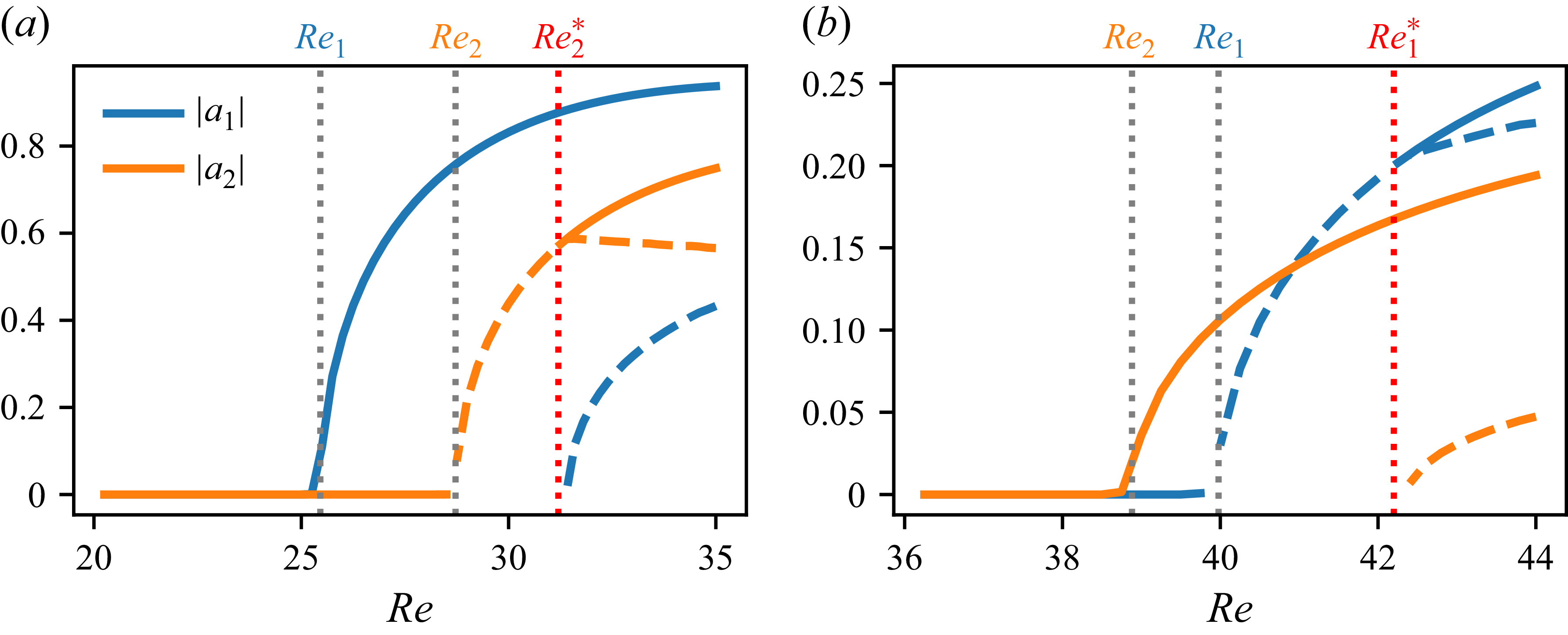
 μ=0.25
 Re1
Re1 Re2
Re2 Re2∗
Re2∗ a1≠0
a1≠0 a2≠0
a2≠0 Re>Re2∗
 μ=1.5
μ=1.5 Re1
Re1 Re1∗
Re1∗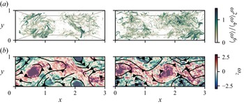
 ω2
ω2 Re=2851
 μ=0.89
 u~⊥(x,y)
 z
z
 Re=2851
 μ=0.89
 E2D
E2D ETS
ETS ER
ER u~⊥
u~⊥ uTS
uTS Ez
Ez uz
uz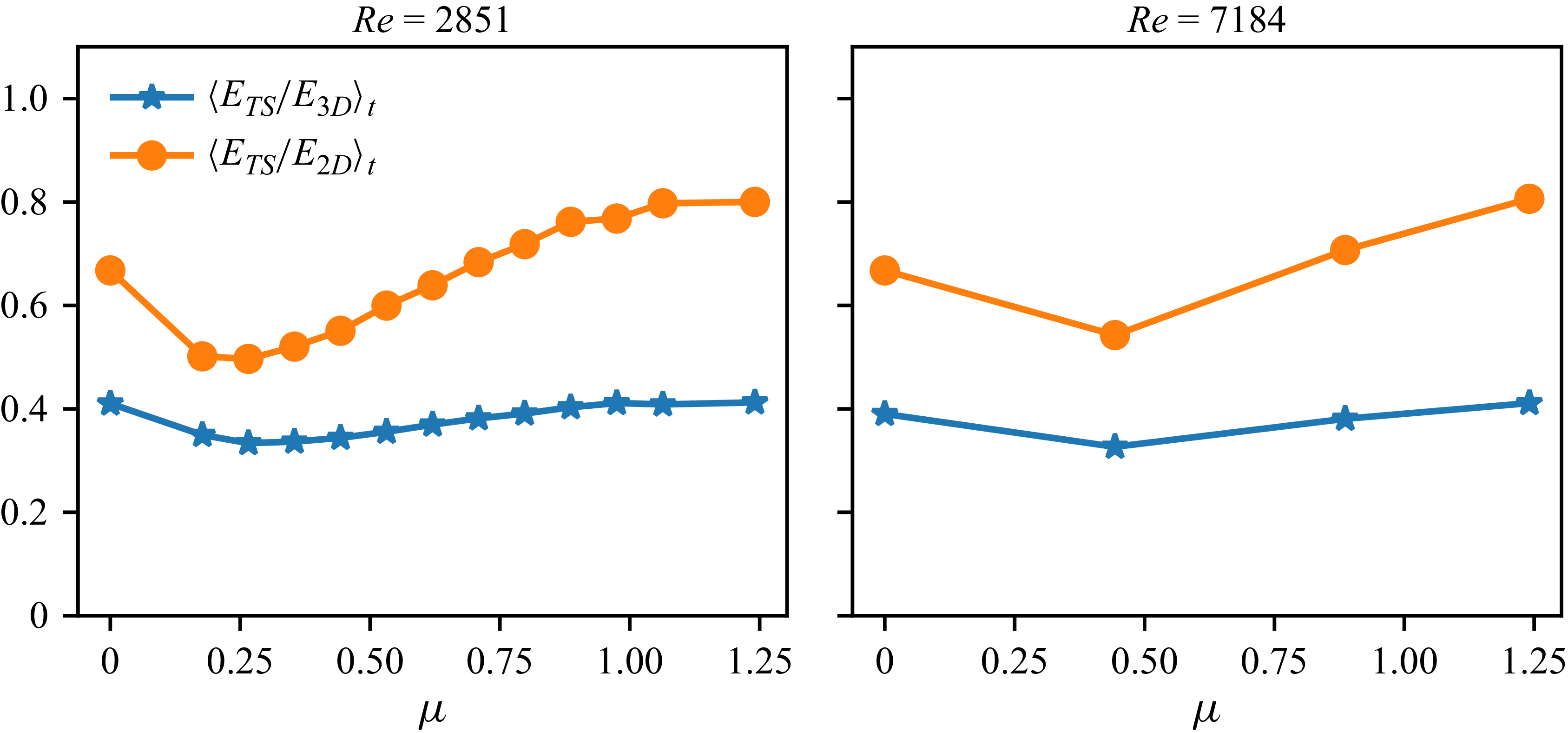
 E3D
E3D E2D
E2D
 A0(t)
A0(t) Re=2851
 μ=0.89
 10T
10T ⟨A0(t)⟩10T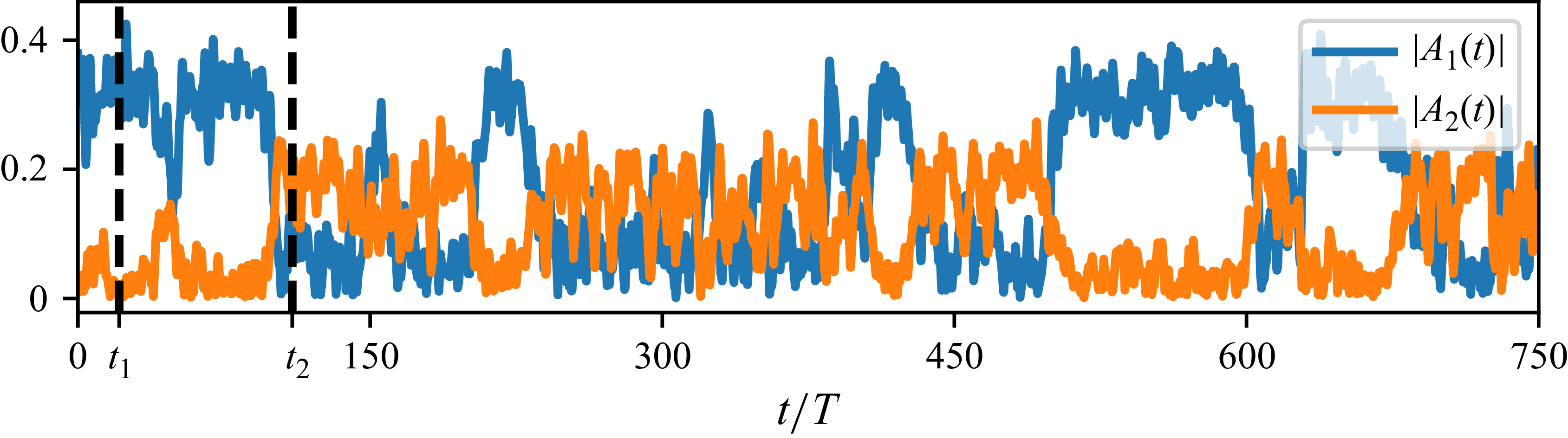
 A1(t)
A1(t) A2(t)
A2(t) Re=2851
 μ=0.89
 (A1,A2)
 Re=2851
 μ=0.89
 Ω1
Ω1 A1
A1 A1mean
 A2
A2 Ω2
Ω2 A2
A2 A2mean
 A1
A1 |A1|
|A1| |A2|
|A2| Ω1
Ω1 Ω2
Ω2
 μ=0.89
 Re=2851
 |A1|
|A1| |A2|
|A2|
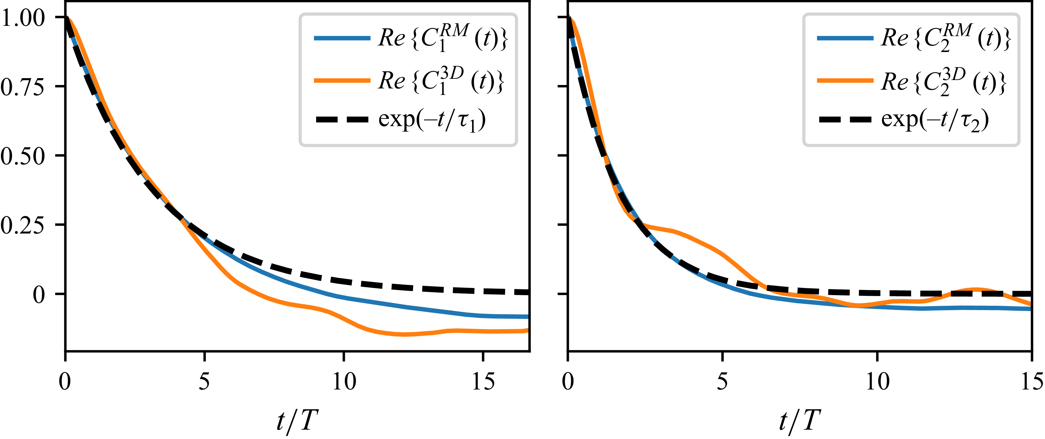
 C13D(t)
 C23D(t)
 Re=2851
 μ=0.89
 C1RM(t)
 C2RM(t)
 μ=0.89
 Re=7184
 C13D(t)
 C23D(t)
 Re=7184
 μ=0.89
 C1RM(t)
 C2RM(t)
 μ
μ
 Open access

