
 α
α α
α





1. Introduction
The Lagrangian-averaged Navier–Stokes- $\alpha$
(LANS
$\alpha$
(LANS $\hbox{-}\alpha$
) equations constitute a turbulence closure model, based on the theory of Lagrangian averaging (Soward Reference Soward1972; Andrews & McIntyre Reference Andrews and McIntyre1978), that has achieved at lower resolution what other more commonly used closure schemes require higher resolution to accomplish in a number of contexts (Chen et al. Reference Chen, Holm, Margolin and Zhang1999; Holm et al. Reference Holm, Jeffery, Kurien, Livescu, Taylor and Wingate2005; Zhao & Mohseni Reference Zhao and Mohseni2005; Geurts & Holm Reference Geurts and Holm2006; Hecht et al. Reference Hecht, Holm, Petersen and Wingate2008a
,
Reference Hecht, Holm, Petersen and Wingateb
). Fundamentally different from classical closure schemes, the LANS-
$\hbox{-}\alpha$
) equations constitute a turbulence closure model, based on the theory of Lagrangian averaging (Soward Reference Soward1972; Andrews & McIntyre Reference Andrews and McIntyre1978), that has achieved at lower resolution what other more commonly used closure schemes require higher resolution to accomplish in a number of contexts (Chen et al. Reference Chen, Holm, Margolin and Zhang1999; Holm et al. Reference Holm, Jeffery, Kurien, Livescu, Taylor and Wingate2005; Zhao & Mohseni Reference Zhao and Mohseni2005; Geurts & Holm Reference Geurts and Holm2006; Hecht et al. Reference Hecht, Holm, Petersen and Wingate2008a
,
Reference Hecht, Holm, Petersen and Wingateb
). Fundamentally different from classical closure schemes, the LANS- $\alpha$
model regularises nonlinear advection rather than introducing an eddy diffusivity. This filters the nonlinear dynamics at length scales smaller than the namesake parameter
$\alpha$
model regularises nonlinear advection rather than introducing an eddy diffusivity. This filters the nonlinear dynamics at length scales smaller than the namesake parameter $\alpha$
. Notably, LANS-
$\alpha$
. Notably, LANS- $\alpha$
produces more energetic simulations over time compared with standard closure schemes (given the same initial energy levels) (Holm & Nadiga Reference Holm and Nadiga2003; Petersen, Hecht & Wingate Reference Petersen, Hecht and Wingate2008), improving the resolution of heat transport, salinity, turbulence statistics and eddy momentum flux in atmosphere and ocean models (Hecht et al. Reference Hecht, Holm, Petersen and Wingate2008b
; Aizinger et al. Reference Aizinger, Korn, Giorgetta and Reich2015; Bennis et al. Reference Bennis, Adong, Boutet and Dumas2021). The characteristic energetic enhancement observed in these applications leads to the central question of this work: can the model’s energetic enhancement be understood through the role of the parameter
$\alpha$
produces more energetic simulations over time compared with standard closure schemes (given the same initial energy levels) (Holm & Nadiga Reference Holm and Nadiga2003; Petersen, Hecht & Wingate Reference Petersen, Hecht and Wingate2008), improving the resolution of heat transport, salinity, turbulence statistics and eddy momentum flux in atmosphere and ocean models (Hecht et al. Reference Hecht, Holm, Petersen and Wingate2008b
; Aizinger et al. Reference Aizinger, Korn, Giorgetta and Reich2015; Bennis et al. Reference Bennis, Adong, Boutet and Dumas2021). The characteristic energetic enhancement observed in these applications leads to the central question of this work: can the model’s energetic enhancement be understood through the role of the parameter $\alpha$
in modifying the underlying wave dynamics and energy transfers?
$\alpha$
in modifying the underlying wave dynamics and energy transfers?
Although this energetic enhancement is a consistent feature of LANS- $\alpha$
across a range of settings, identifying the mechanisms by which it is produced – especially those tied to wave dynamics – is difficult in realistic, large-scale geophysical models. There are partial explanations for why the LANS-
$\alpha$
across a range of settings, identifying the mechanisms by which it is produced – especially those tied to wave dynamics – is difficult in realistic, large-scale geophysical models. There are partial explanations for why the LANS- $\alpha$
model is more energetic; for instance, varying
$\alpha$
model is more energetic; for instance, varying $\alpha$
modifies the dissipation range (Chen et al. Reference Chen, Holm, Margolin and Zhang1999), a property shared by related
$\alpha$
modifies the dissipation range (Chen et al. Reference Chen, Holm, Margolin and Zhang1999), a property shared by related $\alpha$
-regularisation models (Ilyin, Lunasin & Titi Reference Ilyin, Lunasin and Titi2006; Lunasin, Kurien & Titi Reference Lunasin, Kurien and Titi2008). Another contributing mechanism is that LANS-
$\alpha$
-regularisation models (Ilyin, Lunasin & Titi Reference Ilyin, Lunasin and Titi2006; Lunasin, Kurien & Titi Reference Lunasin, Kurien and Titi2008). Another contributing mechanism is that LANS- $\alpha$
introduces an effective Rossby deformation radius that allows baroclinic instability to be resolved at coarser resolution and thereby mimics the conversion of available potential energy to kinetic energy (Holm & Wingate Reference Holm and Wingate2005). However, further insight into the processes driving this increased energy would benefit both the theoretical understanding of the model and its implementation. We thus investigate the energetics of the LANS-
$\alpha$
introduces an effective Rossby deformation radius that allows baroclinic instability to be resolved at coarser resolution and thereby mimics the conversion of available potential energy to kinetic energy (Holm & Wingate Reference Holm and Wingate2005). However, further insight into the processes driving this increased energy would benefit both the theoretical understanding of the model and its implementation. We thus investigate the energetics of the LANS- $\alpha$
model within an idealised setting widely used in studies of rotating stratified turbulence, which is quasi-geostrophic (QG) but retains effects of inertia–gravity waves (e.g. Smith & Waleffe Reference Smith and Waleffe2002). In this way, we can obtain a detailed view of how
$\alpha$
model within an idealised setting widely used in studies of rotating stratified turbulence, which is quasi-geostrophic (QG) but retains effects of inertia–gravity waves (e.g. Smith & Waleffe Reference Smith and Waleffe2002). In this way, we can obtain a detailed view of how $\alpha$
modifies the underlying dynamics.
$\alpha$
modifies the underlying dynamics.
A schematic diagram of the slow and fast dynamics within the fast QG- $\alpha$
limit, for different values of the regularisation parameter
$\alpha$
limit, for different values of the regularisation parameter $\alpha$
. The slow dynamics are illustrated by grey streamlines (over a grey background) and are which become smoother as
$\alpha$
. The slow dynamics are illustrated by grey streamlines (over a grey background) and are which become smoother as $\alpha$
increases, reflecting the role
$\alpha$
increases, reflecting the role $\alpha$
is found to have in the three-dimensional QG-
$\alpha$
is found to have in the three-dimensional QG- $\alpha$
equations (3.10). The fast waves are shown as the dashed black lines distinct from the slow dynamics, and their interaction is symbolised by a star. Although there are fast waves in the
$\alpha$
equations (3.10). The fast waves are shown as the dashed black lines distinct from the slow dynamics, and their interaction is symbolised by a star. Although there are fast waves in the $\alpha =0$
case, for many Burger numbers, there are no interactions between fast waves that contribute to the dynamics until
$\alpha =0$
case, for many Burger numbers, there are no interactions between fast waves that contribute to the dynamics until $\alpha \gt 0$
. The number of interactions increases with
$\alpha \gt 0$
. The number of interactions increases with $\alpha$
, as shown in § 3.4. This modification of the energetic landscape by
$\alpha$
, as shown in § 3.4. This modification of the energetic landscape by $\alpha$
may help to explain why the LANS-
$\alpha$
may help to explain why the LANS- $\alpha$
model is more energetic than other models.
$\alpha$
model is more energetic than other models.

Figure 1. Long description
Figure 1 is a three-panel schematic labelled α = 0, α > 0 small, and α > 0 large. In each panel, the slow dynamics are drawn as a grey curved hypersurface with grey streamlines. The fast dynamics are drawn as dashed oscillating black lines, and wave-wave interactions are marked with black star symbols. From left to right, the slow-dynamics surface appears smoother and the number of star symbols increases. The figure visually indicates that increasing α regularizes the slow dynamics while increasing interactions among fast waves.
The QG equations, originally derived by Charney (Reference Charney1948), describe the large-scale, balanced dynamics primarily driven by planetary rotation. The three-dimensional, continuously stratified system considered here is further constrained by strong background stratification. Specifically, we consider the QG limit $Ro\to 0$
,
$Ro\to 0$
, ${\textit{Fr}}\to 0$
with
${\textit{Fr}}\to 0$
with $F={\textit{Fr}/\textit{Ro}}=f/N$
fixed, following Embid & Majda (Reference Embid and Majda1998), without assuming a small aspect ratio. By design, the QG equations effectively filter out fast, small-scale motions like inertia–gravity waves, isolating the dominant ‘balanced’ flow. The first derivation of the QG limiting dynamics for the Boussinesq-
$F={\textit{Fr}/\textit{Ro}}=f/N$
fixed, following Embid & Majda (Reference Embid and Majda1998), without assuming a small aspect ratio. By design, the QG equations effectively filter out fast, small-scale motions like inertia–gravity waves, isolating the dominant ‘balanced’ flow. The first derivation of the QG limiting dynamics for the Boussinesq- $\alpha$
equations appears in Holm et al. (Reference Holm, Marsden and Ratiu2002), which we extend by presenting the first fast singular limit derivation of QG-
$\alpha$
equations appears in Holm et al. (Reference Holm, Marsden and Ratiu2002), which we extend by presenting the first fast singular limit derivation of QG- $\alpha$
. In our work, the leading-order asymptotic solution is the conservation of PV-
$\alpha$
. In our work, the leading-order asymptotic solution is the conservation of PV- $\alpha$
modulated by the leading-order fast dynamics, which is found by deriving an operator to project the full dynamics onto the null space of the fast operator. Using this framework, we show that the regularisation reshapes the landscape of resonant interactions, both creating a rich structure of interactions purely among fast waves (fast–fast–fast dynamics) that is absent in the unregularised (
$\alpha$
modulated by the leading-order fast dynamics, which is found by deriving an operator to project the full dynamics onto the null space of the fast operator. Using this framework, we show that the regularisation reshapes the landscape of resonant interactions, both creating a rich structure of interactions purely among fast waves (fast–fast–fast dynamics) that is absent in the unregularised ( $\alpha = 0$
) case and substantially altering the number of slow–fast–fast interactions (figure 1). Further, the prognostic variable PV-
$\alpha = 0$
) case and substantially altering the number of slow–fast–fast interactions (figure 1). Further, the prognostic variable PV- $\alpha$
derived in this limit is intrinsically useful for future studies of LANS-
$\alpha$
derived in this limit is intrinsically useful for future studies of LANS- $\alpha$
; it is the central dynamical variable of the balanced system and a quantity fundamental to understanding large-scale geophysical flows (e.g. Charney Reference Charney1948; Rhines & Young Reference Rhines and Young1982; Hoskins, McIntyre & Robertson Reference Hoskins, McIntyre and Robertson1985; Vallis Reference Vallis1996; Holm Reference Holm1999; Julien et al. Reference Julien, Knobloch, Milliff and Werne2006).
$\alpha$
; it is the central dynamical variable of the balanced system and a quantity fundamental to understanding large-scale geophysical flows (e.g. Charney Reference Charney1948; Rhines & Young Reference Rhines and Young1982; Hoskins, McIntyre & Robertson Reference Hoskins, McIntyre and Robertson1985; Vallis Reference Vallis1996; Holm Reference Holm1999; Julien et al. Reference Julien, Knobloch, Milliff and Werne2006).
Charney’s intended elimination of fast dynamics would imply the existence of a ‘slow manifold’, a concept furthered by Leith (Reference Leith1980) and Lorenz (Reference Lorenz1980). Ideally, a reduced system would define this invariant, attracting, lower-dimensional balanced subspace. In practice, this ideal is rarely achieved, and the obtained ‘slow manifolds’ have been instead described as ‘fuzzy’ slow manifolds (Warn & Menard Reference Warn and Menard1986). Even if an original set of equations permits a slow manifold in the mathematical sense, it may not serve as the desired physical slow manifold, e.g. one where gravity wave activity is entirely absent (Lorenz & Krishnamurthy Reference Lorenz and Krishnamurthy1987; Jacobs Reference Jacobs1991; Lorenz Reference Lorenz1992). The QG equations are not strictly invariant: even perfectly balanced initial conditions can spontaneously generate inertia–gravity waves (Vanneste & Yavneh Reference Vanneste and Yavneh2004). While these can be exponentially small given sufficiently smooth flows (Vanneste & Yavneh Reference Vanneste and Yavneh2004; Vanneste Reference Vanneste2013), in fully turbulent rotating stratified flow, imbalance is finite and energetically relevant (see Sutherland et al. (Reference Sutherland, Achatz, Caulfield and Klymak2019) for a review). An unbalanced (ageostrophic) range can emerge spontaneously, eventually dominating the small-scale energy (Kafiabad & Bartello Reference Kafiabad and Bartello2016), with transfer from balanced to unbalanced motions at scales where $Ro$
and
$Ro$
and ${\textit{Fr}}$
are still small (Kafiabad & Bartello Reference Kafiabad and Bartello2018). Fast waves can also emerge even when forcing is applied only to geostrophic modes (Waite Reference Waite2017). Related simulations show divergent (unbalanced) energy far exceeding QG diagnostic estimates (Deusebio, Vallgren & Lindborg Reference Deusebio, Vallgren and Lindborg2013). Furthermore, fast and slow dynamics remain linked through resonant interactions (Ward & Dewar Reference Ward and Dewar2010), even when they are decoupled at leading order. When forcing is not restricted to the slow dynamics, fast motions can strongly affect the system’s energy pathways (Smith & Waleffe Reference Smith and Waleffe2002; Smith & Lee Reference Smith and Lee2005; Whitehead & Wingate Reference Whitehead and Wingate2014). This motivates the general need for reduced models that incorporate the effects of waves and indicates that a robust analysis of the energetics of LANS-
${\textit{Fr}}$
are still small (Kafiabad & Bartello Reference Kafiabad and Bartello2018). Fast waves can also emerge even when forcing is applied only to geostrophic modes (Waite Reference Waite2017). Related simulations show divergent (unbalanced) energy far exceeding QG diagnostic estimates (Deusebio, Vallgren & Lindborg Reference Deusebio, Vallgren and Lindborg2013). Furthermore, fast and slow dynamics remain linked through resonant interactions (Ward & Dewar Reference Ward and Dewar2010), even when they are decoupled at leading order. When forcing is not restricted to the slow dynamics, fast motions can strongly affect the system’s energy pathways (Smith & Waleffe Reference Smith and Waleffe2002; Smith & Lee Reference Smith and Lee2005; Whitehead & Wingate Reference Whitehead and Wingate2014). This motivates the general need for reduced models that incorporate the effects of waves and indicates that a robust analysis of the energetics of LANS- $\alpha$
requires accounting for the fast dynamics.
$\alpha$
requires accounting for the fast dynamics.
To do so, we depart from methods that strictly isolate a slow manifold and instead take a fast singular limit (Klainerman & Majda Reference Klainerman and Majda1981; Majda Reference Majda1984; Babin et al. Reference Babin, Mahalov and Nicolaenko1995; Embid & Majda Reference Embid and Majda1996, Reference Embid and Majda1998; Majda & Embid Reference Majda and Embid1998). By taking the same parameter limit as traditional QG – low Rossby number ( $Ro\to 0$
, geostrophic balance) and low Froude number (
$Ro\to 0$
, geostrophic balance) and low Froude number ( ${\textit{Fr}}\to 0$
, hydrostatic balance), while the ratio between them (
${\textit{Fr}}\to 0$
, hydrostatic balance), while the ratio between them ( $F= {\textit{Fr}/\textit{Ro}}=f/N$
) remains fixed – this approach recovers the standard QG equations for the slow dynamics while retaining fast dynamics at leading order. Applying this process to the LANS-
$F= {\textit{Fr}/\textit{Ro}}=f/N$
) remains fixed – this approach recovers the standard QG equations for the slow dynamics while retaining fast dynamics at leading order. Applying this process to the LANS- $\alpha$
equations yields a system we term the ‘fast QG-
$\alpha$
equations yields a system we term the ‘fast QG- $\alpha$
dynamics’ (or fast QG-
$\alpha$
dynamics’ (or fast QG- $\alpha$
limit). The fast QG-
$\alpha$
limit). The fast QG- $\alpha$
dynamics decompose into the slow dynamics, the balanced geostrophic flow corresponding to the traditional QG equations (but with
$\alpha$
dynamics decompose into the slow dynamics, the balanced geostrophic flow corresponding to the traditional QG equations (but with $\alpha$
regularisation), and the fast dynamics, the inertia–gravity waves filtered out in the traditional limit. The fast dynamics are decoupled from the usual slow dynamics in the sense that the leading-order fast dynamics cannot influence the slow dynamics because these fast, oscillatory effects cancel out when averaged across many wave periods. In this context, the fluctuations about the balanced QG-
$\alpha$
regularisation), and the fast dynamics, the inertia–gravity waves filtered out in the traditional limit. The fast dynamics are decoupled from the usual slow dynamics in the sense that the leading-order fast dynamics cannot influence the slow dynamics because these fast, oscillatory effects cancel out when averaged across many wave periods. In this context, the fluctuations about the balanced QG- $\alpha$
state are the
$\alpha$
state are the $O(1)$
fast dynamics together with all
$O(1)$
fast dynamics together with all $O(\epsilon )$
dynamics, where the small parameter
$O(\epsilon )$
dynamics, where the small parameter $\epsilon$
is taken to be the Rossby number. Physically, the frequency of the fast-wave oscillations is inversely proportional to
$\epsilon$
is taken to be the Rossby number. Physically, the frequency of the fast-wave oscillations is inversely proportional to $\epsilon$
. This approach (Embid & Majda Reference Embid and Majda1996, Reference Embid and Majda1998) is rigorously justified by Schochet’s (1994) method of cancellation of oscillations and may be thought of as averaging over fast waves in geophysical flows. The three-dimensional Boussinesq (or in this work, Boussinesq-
$\epsilon$
. This approach (Embid & Majda Reference Embid and Majda1996, Reference Embid and Majda1998) is rigorously justified by Schochet’s (1994) method of cancellation of oscillations and may be thought of as averaging over fast waves in geophysical flows. The three-dimensional Boussinesq (or in this work, Boussinesq- $\alpha$
) equations admit two kinds of eigenfrequencies: slow (geostrophic) modes (vortical modes) which have zero frequency for all wavenumbers
$\alpha$
) equations admit two kinds of eigenfrequencies: slow (geostrophic) modes (vortical modes) which have zero frequency for all wavenumbers $\boldsymbol{k}$
and fast (ageostrophic) modes (dispersive waves).
$\boldsymbol{k}$
and fast (ageostrophic) modes (dispersive waves).
To understand what drives the LANS- $\alpha$
model’s distinctive energetics, we analyse three-wave resonant and near-resonant interactions. Resonant interactions between slow and fast modes, i.e. interactions between geostrophic turbulence and waves, are a primary mechanism for geostrophic adjustment via a direct cascade of wave energy (Bartello Reference Bartello1995). These resonant interactions are highly dependent on the Burger number (
$\alpha$
model’s distinctive energetics, we analyse three-wave resonant and near-resonant interactions. Resonant interactions between slow and fast modes, i.e. interactions between geostrophic turbulence and waves, are a primary mechanism for geostrophic adjustment via a direct cascade of wave energy (Bartello Reference Bartello1995). These resonant interactions are highly dependent on the Burger number ( ${\textit{Bu}}=Ro^2/{\textit{Fr}}^2$
), which is related to the ratio
${\textit{Bu}}=Ro^2/{\textit{Fr}}^2$
), which is related to the ratio $F=f/N$
via
$F=f/N$
via ${\textit{Bu}}=1/F^2$
. For example, Babin et al. (Reference Babin, Mahalov, Nicolaenko and Zhou1997b
) show analytically that as stratification increases compared with rotation, ageostrophic energy cascades are ‘unfrozen’, allowing nonlinear geostrophic adjustment to occur. With small-scale forcing, geostrophic dynamics dominates at large scales for
${\textit{Bu}}=1/F^2$
. For example, Babin et al. (Reference Babin, Mahalov, Nicolaenko and Zhou1997b
) show analytically that as stratification increases compared with rotation, ageostrophic energy cascades are ‘unfrozen’, allowing nonlinear geostrophic adjustment to occur. With small-scale forcing, geostrophic dynamics dominates at large scales for $1/2\leq F\leq 2$
(or equivalently,
$1/2\leq F\leq 2$
(or equivalently, $1/4\leq Bu\leq 4$
), a range with no triad interactions exclusively involving fast waves (Smith & Waleffe Reference Smith and Waleffe2002). With large-scale forcing, the system transitions from being vortical-energy-dominated for
$1/4\leq Bu\leq 4$
), a range with no triad interactions exclusively involving fast waves (Smith & Waleffe Reference Smith and Waleffe2002). With large-scale forcing, the system transitions from being vortical-energy-dominated for $F\leq 1$
(
$F\leq 1$
( ${\textit{Bu}}\geq 1$
) to being wave-energy-dominated for
${\textit{Bu}}\geq 1$
) to being wave-energy-dominated for $F\gt 1$
(
$F\gt 1$
( ${\textit{Bu}}\lt 1$
) (Sukhatme & Smith Reference Sukhatme and Smith2008). Near-resonant interactions, while more challenging to analyse (Babin, Mahalov & Nicolaenko Reference Babin, Mahalov and Nicolaenko1999) and weak for
${\textit{Bu}}\lt 1$
) (Sukhatme & Smith Reference Sukhatme and Smith2008). Near-resonant interactions, while more challenging to analyse (Babin, Mahalov & Nicolaenko Reference Babin, Mahalov and Nicolaenko1999) and weak for $F\sim O(1)$
(Babin, Mahalov & Nicolaenko Reference Babin, Mahalov and Nicolaenko2002), also play an important role in the transfer of energy to slow modes (Smith & Lee Reference Smith and Lee2005). Many geophysical flows have
$F\sim O(1)$
(Babin, Mahalov & Nicolaenko Reference Babin, Mahalov and Nicolaenko2002), also play an important role in the transfer of energy to slow modes (Smith & Lee Reference Smith and Lee2005). Many geophysical flows have $N/f\gg 1$
(
$N/f\gg 1$
( $F\ll 1$
); for example,
$F\ll 1$
); for example, $f/N$
is typically
$f/N$
is typically $O(10^{-2})$
in the mid-latitude atmosphere and
$O(10^{-2})$
in the mid-latitude atmosphere and $O(10^{-1})$
in the deep ocean. Our focus on
$O(10^{-1})$
in the deep ocean. Our focus on $F=O(1)$
isolates a regime in which exact fast-wave-only resonances are absent for
$F=O(1)$
isolates a regime in which exact fast-wave-only resonances are absent for $\alpha =0$
, making
$\alpha =0$
, making $\alpha$
-induced changes to wave–wave pathways especially transparent. Outside this range, the resonant and near-resonant interaction landscape is far less constrained (see also Smith & Waleffe (Reference Smith and Waleffe2002), for
$\alpha$
-induced changes to wave–wave pathways especially transparent. Outside this range, the resonant and near-resonant interaction landscape is far less constrained (see also Smith & Waleffe (Reference Smith and Waleffe2002), for $N/f=10$
and
$N/f=10$
and $100$
).
$100$
).
Our numerical simulations reveal that the smoothing parameter $\alpha$
plays a role analogous to that of the rotation-to-stratification ratio
$\alpha$
plays a role analogous to that of the rotation-to-stratification ratio $F$
and affects wave–vortex energy ratios in a similar manner. However, a key difference emerges when varying
$F$
and affects wave–vortex energy ratios in a similar manner. However, a key difference emerges when varying $\alpha$
as opposed to
$\alpha$
as opposed to $F$
(or
$F$
(or ${\textit{Bu}}$
): increasing
${\textit{Bu}}$
): increasing $\alpha$
markedly extends the persistence of wave energy, thereby slowing the typical transition to vortical energy dominance. A likely mechanism for this is found in how
$\alpha$
markedly extends the persistence of wave energy, thereby slowing the typical transition to vortical energy dominance. A likely mechanism for this is found in how $\alpha$
reshapes three-wave resonant interactions. In the standard fast QG limit, resonant interactions in which two fast waves produce another fast wave are non-existent for many Burger numbers and sparse otherwise. In contrast, by numerically tabulating how often our analytically derived eigenfrequencies satisfy the condition for resonance interactions, we find that
$\alpha$
reshapes three-wave resonant interactions. In the standard fast QG limit, resonant interactions in which two fast waves produce another fast wave are non-existent for many Burger numbers and sparse otherwise. In contrast, by numerically tabulating how often our analytically derived eigenfrequencies satisfy the condition for resonance interactions, we find that $\alpha$
-regularisation drastically increases the number of these interactions (as illustrated in figure 1). While
$\alpha$
-regularisation drastically increases the number of these interactions (as illustrated in figure 1). While $\alpha$
was previously known to modify the dissipation range, these alterations to the triad interactions reveal that the introduction of
$\alpha$
was previously known to modify the dissipation range, these alterations to the triad interactions reveal that the introduction of $\alpha$
can both cause energy to accumulate within the waves and decrease resonant interactions generally responsible for cross-scale energy transfer, providing a mechanism by which energy may be prevented from reaching dissipative scales and thus accumulate within the system. Collectively, our results indicate that LANS-
$\alpha$
can both cause energy to accumulate within the waves and decrease resonant interactions generally responsible for cross-scale energy transfer, providing a mechanism by which energy may be prevented from reaching dissipative scales and thus accumulate within the system. Collectively, our results indicate that LANS- $\alpha$
is likely more energetic than other models because of the way
$\alpha$
is likely more energetic than other models because of the way $\alpha$
-regularisation modulates fast waves, affecting their persistence and ability to satisfy resonance conditions that drive energy transfer among the slow and fast components of the flow.
$\alpha$
-regularisation modulates fast waves, affecting their persistence and ability to satisfy resonance conditions that drive energy transfer among the slow and fast components of the flow.
The remainder of this paper is organised as follows. In § 2, we introduce the LANS- $\alpha$
equations, including their non-dimensional, non-local form, and interpretation as Lagrangian-averaged Navier–Stokes. The derivation of the fast QG limit for LANS-
$\alpha$
equations, including their non-dimensional, non-local form, and interpretation as Lagrangian-averaged Navier–Stokes. The derivation of the fast QG limit for LANS- $\alpha$
is presented in § 3; this section includes energy conservation laws, the slow dynamics (conservation of PV-
$\alpha$
is presented in § 3; this section includes energy conservation laws, the slow dynamics (conservation of PV- $\alpha$
), the fast limiting dynamics (
$\alpha$
), the fast limiting dynamics ( $O(1)$
wave dynamics) and an analysis of how the parameter
$O(1)$
wave dynamics) and an analysis of how the parameter $\alpha$
modifies three-wave resonance interactions. In § 4, we present numerical simulations focusing on the evolution of slow and wave energies in the QG limit and how it depends on
$\alpha$
modifies three-wave resonance interactions. In § 4, we present numerical simulations focusing on the evolution of slow and wave energies in the QG limit and how it depends on $\alpha$
. Finally, in § 5, we discuss the main findings and their broader implications.
$\alpha$
. Finally, in § 5, we discuss the main findings and their broader implications.
2. The LANS- $\alpha$
equations
$\alpha$
equations

2.1. Non-local form of the LANS-
$\alpha$
equations

The LANS- $\alpha$
equations with the Boussinesq approximation (the Boussinesq-
$\alpha$
equations with the Boussinesq approximation (the Boussinesq- $\alpha$
equations) are given by (Holm Reference Holm1999; Holm & Titi Reference Holm and Titi2005)
$\alpha$
equations) are given by (Holm Reference Holm1999; Holm & Titi Reference Holm and Titi2005)
 \begin{align} \frac {\partial \boldsymbol{v}}{\partial t} + \boldsymbol{u} \boldsymbol{\cdot }\boldsymbol{\nabla }\boldsymbol{v} + \boldsymbol{v}\boldsymbol{\cdot }\boldsymbol{\nabla }\boldsymbol{u}^T + f\hat {\boldsymbol{z}}\times \boldsymbol{u} + \boldsymbol{\nabla }\phi +\frac {\rho }{\rho _0}g\hat {\boldsymbol{z}} &= \mathscr{D}_{\nu }\boldsymbol{v} + \mathcal{F}, \end{align}
 \begin{align} \frac {\partial \rho }{\partial t} + \boldsymbol{u} \boldsymbol{\cdot }\boldsymbol{\nabla }\rho -\boldsymbol{u}\boldsymbol{\cdot }b\hat {\boldsymbol{z}} &=\mathscr{D}_\kappa \rho , \end{align}
 \begin{align} \boldsymbol{\nabla }\boldsymbol{\cdot }\boldsymbol{u} &= 0, \end{align}
 \begin{align} \boldsymbol{v} &= \boldsymbol{u} - \alpha ^2 \Delta \boldsymbol{u}, \end{align}
where $\boldsymbol{v}=(v_1,v_2,v_3)$
is the three-dimensional velocity,
$\boldsymbol{v}=(v_1,v_2,v_3)$
is the three-dimensional velocity, $f$
is the Coriolis parameter,
$f$
is the Coriolis parameter, $\phi$
is a modified pressure,
$\phi$
is a modified pressure, $\rho$
is the buoyancy variable (density),
$\rho$
is the buoyancy variable (density), $\rho _0$
is a reference density,
$\rho _0$
is a reference density, $g$
is the gravitational constant,
$g$
is the gravitational constant, $b$
is the strength of the underlying density stratification,
$b$
is the strength of the underlying density stratification, $\alpha \in \mathbb{R}$
is a parameter with units of length,
$\alpha \in \mathbb{R}$
is a parameter with units of length, $\mathcal{F}$
is a forcing term and
$\mathcal{F}$
is a forcing term and $\mathscr{D}_\nu$
and
$\mathscr{D}_\nu$
and $\mathscr{D}_\kappa$
are diffusive operators. For the theoretical developments of this work, we will set these to the usual
$\mathscr{D}_\kappa$
are diffusive operators. For the theoretical developments of this work, we will set these to the usual $\mathscr{D}_\nu \boldsymbol{v} =\nu \Delta \boldsymbol{v}$
and
$\mathscr{D}_\nu \boldsymbol{v} =\nu \Delta \boldsymbol{v}$
and $\mathscr{D}_\kappa \rho = \kappa \Delta \rho$
, where
$\mathscr{D}_\kappa \rho = \kappa \Delta \rho$
, where $\nu$
is the viscosity coefficient and
$\nu$
is the viscosity coefficient and $\kappa$
is buoyancy diffusivity, but will use hyperviscosity in the simulations done in § 4, as this is a standard method to increase the inertial range (see e.g. Smith & Waleffe Reference Smith and Waleffe2002).
$\kappa$
is buoyancy diffusivity, but will use hyperviscosity in the simulations done in § 4, as this is a standard method to increase the inertial range (see e.g. Smith & Waleffe Reference Smith and Waleffe2002).
While the length scale $\alpha$
can be interpreted in many ways – such as the typical deviation of a particle trajectory from its time-averaged path (Holm et al. Reference Holm, Jeffery, Kurien, Livescu, Taylor and Wingate2005) or a filter width (Lunasin et al. Reference Lunasin, Kurien, Taylor and Titi2007) – we adopt the interpretation that it is the length scale below which the dynamics is regularised. This regularisation is accomplished through the introduction of a new velocity field,
$\alpha$
can be interpreted in many ways – such as the typical deviation of a particle trajectory from its time-averaged path (Holm et al. Reference Holm, Jeffery, Kurien, Livescu, Taylor and Wingate2005) or a filter width (Lunasin et al. Reference Lunasin, Kurien, Taylor and Titi2007) – we adopt the interpretation that it is the length scale below which the dynamics is regularised. This regularisation is accomplished through the introduction of a new velocity field, $\boldsymbol{u}=(u_1, u_2, u_3)$
, as defined in (2.1d
) (note that
$\boldsymbol{u}=(u_1, u_2, u_3)$
, as defined in (2.1d
) (note that $\alpha ^2\geq 0$
). Since the advecting velocity is regularised, the development of sharp gradients at scales smaller than
$\alpha ^2\geq 0$
). Since the advecting velocity is regularised, the development of sharp gradients at scales smaller than $\alpha$
is mitigated. The field
$\alpha$
is mitigated. The field $\boldsymbol{v}$
is referred to as the associated circulation velocity, i.e. the quantity whose line integral appears in the Kelvin circulation theorem along loops transported by
$\boldsymbol{v}$
is referred to as the associated circulation velocity, i.e. the quantity whose line integral appears in the Kelvin circulation theorem along loops transported by $\boldsymbol{u}$
(see e.g. Holm & Titi Reference Holm and Titi2005). The relationship between
$\boldsymbol{u}$
(see e.g. Holm & Titi Reference Holm and Titi2005). The relationship between $\boldsymbol{u}$
and
$\boldsymbol{u}$
and $\boldsymbol{v}$
in (2.1d
) can be otherwise interpreted within the Lagrangian-averaging closure; we summarise this interpretation below.
$\boldsymbol{v}$
in (2.1d
) can be otherwise interpreted within the Lagrangian-averaging closure; we summarise this interpretation below.
The difference between the Boussinesq- $\alpha$
equations and the usual Boussinesq equations is essentially due to the use of
$\alpha$
equations and the usual Boussinesq equations is essentially due to the use of $\boldsymbol{u}$
as the transport velocity. Denoting the Helmholtz operator as
$\boldsymbol{u}$
as the transport velocity. Denoting the Helmholtz operator as
 \begin{equation} \mathcal{S}\overset {{\text{def}}}{=} \big(1-\alpha ^2\varDelta \big), \end{equation} $\boldsymbol{u}$
is constructed via
$\boldsymbol{u}$
is constructed via $\mathcal{S}^{-1}\boldsymbol{v}$
(2.1d
). This results in an additional advective term,
$\mathcal{S}^{-1}\boldsymbol{v}$
(2.1d
). This results in an additional advective term, $\boldsymbol{v} \boldsymbol{\cdot }\boldsymbol{\nabla }\boldsymbol{u}^T$
(also written as
$\boldsymbol{v} \boldsymbol{\cdot }\boldsymbol{\nabla }\boldsymbol{u}^T$
(also written as $(\boldsymbol{\nabla }\boldsymbol{u})^T \boldsymbol{v}$
or
$(\boldsymbol{\nabla }\boldsymbol{u})^T \boldsymbol{v}$
or $v_j\partial _i u_j$
), in (2.1a
) and necessitates a modification to the pressure. The usual pressure
$v_j\partial _i u_j$
), in (2.1a
) and necessitates a modification to the pressure. The usual pressure $p$
has been replaced with the modified pressure
$p$
has been replaced with the modified pressure $\phi$
in (2.1a
), where
$\phi$
in (2.1a
), where
 \begin{equation} \phi \overset {{\text{def}}}{=} \frac {p}{\rho _0} - \frac {1}{2}|\boldsymbol{u}|^2-\frac {\alpha ^2}{2}|\boldsymbol{\nabla }\boldsymbol{u}|^2. \end{equation}
From the definition of $\mathcal{S}$
(2.2), the incompressibility of
$\mathcal{S}$
(2.2), the incompressibility of $\boldsymbol{u}$
implies that of
$\boldsymbol{u}$
implies that of $\boldsymbol{v}$
, and vice versa, since the order of the divergence and the Laplacian can be interchanged. Note also that
$\boldsymbol{v}$
, and vice versa, since the order of the divergence and the Laplacian can be interchanged. Note also that $\mathcal{S}$
can be applied to scalar functions, with the interpretation that
$\mathcal{S}$
can be applied to scalar functions, with the interpretation that $\varDelta$
is the scalar Laplacian rather than the vector Laplacian. Using the Helmholtz operator to modify the advecting velocity does not introduce dissipative effects, since (2.1a
) and (2.1b
) are time-reversible when
$\varDelta$
is the scalar Laplacian rather than the vector Laplacian. Using the Helmholtz operator to modify the advecting velocity does not introduce dissipative effects, since (2.1a
) and (2.1b
) are time-reversible when $\nu =\kappa =0$
.
$\nu =\kappa =0$
.
In (2.1a – d ), the density has been decomposed as
 \begin{equation} \rho _{\textit{full}} = \overline {\rho }+\rho , \quad \overline {\rho } = \rho _0 - bz, \quad b\gt 0. \end{equation}
The domain is $[0,L]^3$
, for a length scale
$[0,L]^3$
, for a length scale $L$
, with triply periodic boundary conditions, to facilitate the comparison of the results presented here with those of previous turbulence studies and the classical fast singular QG limit (Embid & Majda Reference Embid and Majda1998).
$L$
, with triply periodic boundary conditions, to facilitate the comparison of the results presented here with those of previous turbulence studies and the classical fast singular QG limit (Embid & Majda Reference Embid and Majda1998).
We non-dimensionalise the Boussinesq- $\alpha$
equations by considering a characteristic length scale
$\alpha$
equations by considering a characteristic length scale $L$
(e.g. the domain length) and velocity scale
$L$
(e.g. the domain length) and velocity scale $U$
, which correspond to the advective time scale
$U$
, which correspond to the advective time scale $L/U$
. Using the Brunt–Väisälä frequency
$L/U$
. Using the Brunt–Väisälä frequency $N=(gb/\rho _0)^{1/2}$
, we define the buoyancy fluctuation scale
$N=(gb/\rho _0)^{1/2}$
, we define the buoyancy fluctuation scale $B=NU/g$
in order to non-dimensionalise the density fluctuations. Note that throughout this work,
$B=NU/g$
in order to non-dimensionalise the density fluctuations. Note that throughout this work, $N$
is considered constant. We non-dimensionalise
$N$
is considered constant. We non-dimensionalise $\boldsymbol{x}'=\boldsymbol{x}/L$
,
$\boldsymbol{x}'=\boldsymbol{x}/L$
, $t'=t/T$
,
$t'=t/T$
, $\boldsymbol{v'}=\boldsymbol{v}/U$
,
$\boldsymbol{v'}=\boldsymbol{v}/U$
, $\rho '=\rho /(\rho _0 B)$
and the pressure via
$\rho '=\rho /(\rho _0 B)$
and the pressure via $p'=p/\overline {p}$
, where
$p'=p/\overline {p}$
, where $\overline {p}$
is a reference pressure (cf. Majda Reference Majda2003). Using these scalings, the Rossby, Froude, Reynolds, Prandtl and Euler numbers arise naturally:
$\overline {p}$
is a reference pressure (cf. Majda Reference Majda2003). Using these scalings, the Rossby, Froude, Reynolds, Prandtl and Euler numbers arise naturally:
 \begin{equation} {\textit{Ro}} \overset {{\text{def}}}{=} \frac {U}{\textit{fL}}, \quad {\textit{Fr}} \overset {{\text{def}}}{=} \frac {U}{NL}, \quad Re \overset {{\text{def}}}{=} \frac {\rho _0UL}{\nu }, \quad Pr \overset {{\text{def}}}{=} \frac {\nu }{\rho _0\kappa }, \quad Eu \overset {{\text{def}}}{=} \frac {\overline {p}}{\rho _0 U^2}. \end{equation}
The parameter $F$
, which measures the relative strength of rotation versus stratification,
$F$
, which measures the relative strength of rotation versus stratification,
 \begin{equation} F\overset {{\text{def}}}{=} \frac {\textit{Fr}}{\textit{Ro}}=\frac {f}{N}, \end{equation}
also arises in the system and must be assumed fixed when taking the QG limit. This parameter is closely related to the Burger number
 \begin{equation} Bu\overset {{\text{def}}}{=} \frac {Ro^2}{{\textit{Fr}}^2}=\frac {1}{F^2}, \end{equation}
and plays an important role in the dynamics.
Omitting the primes, the non-dimensionalised version of (2.1) is given by
 \begin{align} \frac {\partial \boldsymbol{v}}{\partial t} + \boldsymbol{u}\boldsymbol{\cdot }\boldsymbol{\nabla }\boldsymbol{v} +\boldsymbol{v} \boldsymbol{\cdot }\boldsymbol{\nabla }\boldsymbol{u}^T+ \frac {1}{\textit{Ro}} \hat {\boldsymbol{z}} \times \boldsymbol{u} + \boldsymbol{\nabla }\phi + \frac {1}{\textit{Fr}}\rho \hat {\boldsymbol{z}} &= \frac {1}{\textit{Re}}\Delta \boldsymbol{v}+\mathcal{F}, \end{align}
 \begin{align} \frac {\partial \rho }{\partial t} + \boldsymbol{u}\boldsymbol{\cdot }\boldsymbol{\nabla }\rho - \frac {1}{\textit{Fr}}\boldsymbol{u}\boldsymbol{\cdot }\hat {\boldsymbol{z}} &= \frac {1}{\textit{RePr}}\Delta \rho , \end{align}
 \begin{align} \boldsymbol{\nabla }\boldsymbol{\cdot }\boldsymbol{u} &= 0, \end{align}
 \begin{align} \boldsymbol{u}&=\mathcal{S}^{-1}\boldsymbol{v}, \end{align}
 \begin{align} \boldsymbol{\nabla }\varDelta ^{-1}\left (\frac {1}{\textit{Ro}}\hat {\boldsymbol{z}}\boldsymbol{\cdot }\mathcal{S}^{-1} \boldsymbol{\omega } -\boldsymbol{\nabla }\boldsymbol{\cdot }(\mathcal{S}^{-1}\boldsymbol{v}\boldsymbol{\cdot }\boldsymbol{\nabla }\boldsymbol{v} + \boldsymbol{v} \boldsymbol{\cdot }\boldsymbol{\nabla }(\mathcal{S}^{-1}\boldsymbol{v})^T)-\frac {1}{\textit{Fr}}\frac {\partial \rho }{\partial z}\right )&=\boldsymbol{\nabla }\phi . \end{align}
Here, the vorticity $\boldsymbol{\omega }\overset {{\text{def}}}{=} \boldsymbol{\nabla }\times \boldsymbol{v}$
and
$\boldsymbol{\omega }\overset {{\text{def}}}{=} \boldsymbol{\nabla }\times \boldsymbol{v}$
and $\mathcal{S}$
is actually the non-dimensionalised Helmholtz operator,
$\mathcal{S}$
is actually the non-dimensionalised Helmholtz operator, $(1-L_\alpha \Delta )$
, where
$(1-L_\alpha \Delta )$
, where $L_\alpha \overset {{\text{def}}}{=} \alpha ^2/L^2$
. Since
$L_\alpha \overset {{\text{def}}}{=} \alpha ^2/L^2$
. Since $\alpha$
is a fraction of the domain length, and we use the domain size as the characteristic length scale,
$\alpha$
is a fraction of the domain length, and we use the domain size as the characteristic length scale, $L_\alpha \in [0,1]$
. The modified pressure
$L_\alpha \in [0,1]$
. The modified pressure $\phi$
and forcing
$\phi$
and forcing $\mathcal{F}$
are also the non-dimensional versions. The scalings
$\mathcal{F}$
are also the non-dimensional versions. The scalings $BgLU^{-2} = (Fr)^{-1}$
and
$BgLU^{-2} = (Fr)^{-1}$
and $Eu=(Ro)^{-1}$
have been used in (2.8) (Majda Reference Majda2003, § 7.4). The non-local form of the momentum equations is found by solving the elliptic equation for the modified pressure, i.e. replacing
$Eu=(Ro)^{-1}$
have been used in (2.8) (Majda Reference Majda2003, § 7.4). The non-local form of the momentum equations is found by solving the elliptic equation for the modified pressure, i.e. replacing $\boldsymbol{\nabla }\phi$
in (2.8a
) with (2.8e
). The modified pressure thus does not further differentiate the Boussinesq-
$\boldsymbol{\nabla }\phi$
in (2.8a
) with (2.8e
). The modified pressure thus does not further differentiate the Boussinesq- $\alpha$
equations from the unregularised Boussinesq equations;
$\alpha$
equations from the unregularised Boussinesq equations; $\phi$
is a free variable in exactly the same sense that
$\phi$
is a free variable in exactly the same sense that $p$
is.
$p$
is.
This system reduces to the usual Boussinesq equations in the case of $\alpha =0$
, so we expect the slow and fast dynamics derived for the LANS-
$\alpha =0$
, so we expect the slow and fast dynamics derived for the LANS- $\alpha$
model to reduce to those found in Embid & Majda (Reference Embid and Majda1998), Babin et al. (Reference Babin, Mahalov, Nicolaenko and Zhou1997b
) and Wingate et al. (Reference Wingate, Embid, Holmes-Cerfon and Taylor2011) when
$\alpha$
model to reduce to those found in Embid & Majda (Reference Embid and Majda1998), Babin et al. (Reference Babin, Mahalov, Nicolaenko and Zhou1997b
) and Wingate et al. (Reference Wingate, Embid, Holmes-Cerfon and Taylor2011) when $\alpha =0$
.
$\alpha =0$
.
The LANS- $\alpha$
equations may be viewed as a Lagrangian-averaged closure formulated within the Euler–Poincaré variational framework (Holm, Marsden & Ratiu Reference Holm, Marsden and Ratiu1998; Holm Reference Holm1999). In common with generalised Lagrangian mean (GLM) theory (Andrews & McIntyre Reference Andrews and McIntyre1978), the circulation velocity
$\alpha$
equations may be viewed as a Lagrangian-averaged closure formulated within the Euler–Poincaré variational framework (Holm, Marsden & Ratiu Reference Holm, Marsden and Ratiu1998; Holm Reference Holm1999). In common with generalised Lagrangian mean (GLM) theory (Andrews & McIntyre Reference Andrews and McIntyre1978), the circulation velocity $\boldsymbol{v}$
is advected by the transport velocity
$\boldsymbol{v}$
is advected by the transport velocity $\boldsymbol{u}$
, which is identified with the Lagrangian-mean velocity. Closure of the Lagrangian-averaged system requires independently prescribing the covariance of particle displacement fluctuations
$\boldsymbol{u}$
, which is identified with the Lagrangian-mean velocity. Closure of the Lagrangian-averaged system requires independently prescribing the covariance of particle displacement fluctuations $\langle \boldsymbol{\xi }\boldsymbol{\xi }\rangle$
, where
$\langle \boldsymbol{\xi }\boldsymbol{\xi }\rangle$
, where $\boldsymbol{\xi }$
denotes a rapid fluctuation of a fluid parcel trajectory; this covariance enters through a general operator
$\boldsymbol{\xi }$
denotes a rapid fluctuation of a fluid parcel trajectory; this covariance enters through a general operator $\tilde {\Delta } = \boldsymbol{\nabla }\boldsymbol{\cdot }\langle \boldsymbol{\xi }\boldsymbol{\xi }\rangle \boldsymbol{\cdot }\boldsymbol{\nabla}$
that governs the relationship between
$\tilde {\Delta } = \boldsymbol{\nabla }\boldsymbol{\cdot }\langle \boldsymbol{\xi }\boldsymbol{\xi }\rangle \boldsymbol{\cdot }\boldsymbol{\nabla}$
that governs the relationship between $\boldsymbol{u}$
and
$\boldsymbol{u}$
and $\boldsymbol{v}$
in the full Lagrangian-averaged system (Holm Reference Holm1999). The Helmholtz operator
$\boldsymbol{v}$
in the full Lagrangian-averaged system (Holm Reference Holm1999). The Helmholtz operator $\mathcal{S}$
is an isotropic approximation of this operator. Specifically, the isotropy condition
$\mathcal{S}$
is an isotropic approximation of this operator. Specifically, the isotropy condition $\langle \xi ^k \xi ^l\rangle = \alpha ^2 \delta ^{kl}$
, where
$\langle \xi ^k \xi ^l\rangle = \alpha ^2 \delta ^{kl}$
, where $\alpha$
is constant if the statistics are homogeneous, reduces
$\alpha$
is constant if the statistics are homogeneous, reduces $\tilde {\Delta }$
to
$\tilde {\Delta }$
to $\alpha ^2 \Delta$
and yields (2.1d
). In GLM theory, the standard interpretation identifies the circulation velocity with the difference between the Lagrangian-mean velocity and the pseudo-momentum (Andrews & McIntyre Reference Andrews and McIntyre1978; Gilbert & Vanneste Reference Gilbert and Vanneste2018).
$\alpha ^2 \Delta$
and yields (2.1d
). In GLM theory, the standard interpretation identifies the circulation velocity with the difference between the Lagrangian-mean velocity and the pseudo-momentum (Andrews & McIntyre Reference Andrews and McIntyre1978; Gilbert & Vanneste Reference Gilbert and Vanneste2018).
Interpreting the LANS- $\alpha$
system as Lagrangian-averaged Navier–Stokes in this way, this closure allows the Helmholtz operator
$\alpha$
system as Lagrangian-averaged Navier–Stokes in this way, this closure allows the Helmholtz operator $\mathcal{S}$
to be commuted with the advective operator, a key property used in the derivation of the slow dynamics. While it is by now standard to regularise Navier–Stokes by applying a number of different filters, this particular filter, with the given meaning of
$\mathcal{S}$
to be commuted with the advective operator, a key property used in the derivation of the slow dynamics. While it is by now standard to regularise Navier–Stokes by applying a number of different filters, this particular filter, with the given meaning of $\alpha$
, is especially advantageous due to its commutative properties with space and time derivatives and advection.
$\alpha$
, is especially advantageous due to its commutative properties with space and time derivatives and advection.
3. The fast QG limit of the LANS-
$\alpha$
equations

3.1. Abstract framework
As in Embid & Majda (Reference Embid and Majda1996, Reference Embid and Majda1998), Babin et al. (Reference Babin, Mahalov, Nicolaenko and Zhou1997b ), Wingate et al. (Reference Wingate, Embid, Holmes-Cerfon and Taylor2011) and Whitehead & Wingate (Reference Whitehead and Wingate2014), we write the dependent variables as a vector:
 \begin{equation} \boldsymbol{w} \overset {{\text{def}}}{=} \begin{pmatrix} \boldsymbol{v} \\ \rho \end{pmatrix}. \end{equation}
The non-dimensionalised LANS- $\alpha$
equations (2.8) may then be rewritten in the abstract operator form:
$\alpha$
equations (2.8) may then be rewritten in the abstract operator form:
 \begin{equation} \frac {\partial \boldsymbol{w}}{\partial t} + \frac {1}{\textit{Ro}}\mathcal{L}_{\textit{Ro}}\boldsymbol{w} + \frac {1}{\textit{Fr}}\mathcal{L}_{\textit{Fr}}\boldsymbol{w} + \mathcal{B}(\boldsymbol{w},\boldsymbol{w}) = \mathcal{D}\boldsymbol{w} \end{equation}
(omitting any forcing, as in Embid & Majda (Reference Embid and Majda1998)). In (3.2), the operators are defined:
 \begin{align} \mathcal{L}_{\textit{Ro}} \boldsymbol{w} &= \begin{pmatrix}\mathcal{S}^{-1}\Big (\boldsymbol{v}_H^\perp + \boldsymbol{\nabla} _H \varDelta ^{-1} \left (\hat {\boldsymbol{z}}\boldsymbol{\cdot }(\boldsymbol{\nabla }\times \boldsymbol{v})\right )\Big ) \\[8pt] \mathcal{S}^{-1}\Big (\dfrac {\partial }{\partial z}\varDelta ^{-1}(\hat {\boldsymbol{z}}\boldsymbol{\cdot }(\boldsymbol{\nabla }\times \boldsymbol{v}))\Big ) \\[5pt] 0 \end{pmatrix}, \notag\\ \mathcal{L}_{\textit{Fr}}\boldsymbol{w} &= \begin{pmatrix} - \boldsymbol{\nabla} _H \varDelta ^{-1}\left (\dfrac {\partial \rho }{\partial z}\right ) \notag\\[12pt] -\varDelta ^{-1}\left (\dfrac {\partial ^2\rho }{\partial z^2} \right )+ \rho \\[12pt] -\mathcal{S}^{-1}v_3 \end{pmatrix},\notag\\ \mathcal{B}(\boldsymbol{w}, \boldsymbol{w}) &= \begin{pmatrix} \big(\mathcal{S}^{-1} \boldsymbol{v} \boldsymbol{\cdot }\boldsymbol{\nabla }\big) \boldsymbol{v} - \boldsymbol{\nabla }\varDelta ^{-1}\Big (\boldsymbol{\nabla }\boldsymbol{\cdot }\Big(\big(\mathcal{S}^{-1} \boldsymbol{v} \boldsymbol{\cdot }\boldsymbol{\nabla }\big) \boldsymbol{v}+ \boldsymbol{v} \boldsymbol{\cdot }\boldsymbol{\nabla }(\mathcal{S}^{-1}\boldsymbol{v})^T\Big)\Big ) \\[6pt] (\mathcal{S}^{-1}\boldsymbol{v}\boldsymbol{\cdot }\boldsymbol{\nabla }) \rho \end{pmatrix},\notag \\ \mathcal{D}\boldsymbol{w} &= \frac {1}{\textit{Re}}\begin{pmatrix} \Delta \boldsymbol{v} \\[5pt] \dfrac {1}{Pr}\Delta \rho \end{pmatrix}. \end{align}
To write the operators in this form, we made use of the commutative properties of $\mathcal{S}$
. Each of these operators reduces to those in Embid & Majda (Reference Embid and Majda1998), Babin et al. (Reference Babin, Mahalov, Nicolaenko and Zhou1997b
) and Wingate et al. (Reference Wingate, Embid, Holmes-Cerfon and Taylor2011) in the case of
$\mathcal{S}$
. Each of these operators reduces to those in Embid & Majda (Reference Embid and Majda1998), Babin et al. (Reference Babin, Mahalov, Nicolaenko and Zhou1997b
) and Wingate et al. (Reference Wingate, Embid, Holmes-Cerfon and Taylor2011) in the case of $\alpha =0$
.
$\alpha =0$
.
We decompose the full solution to (3.2), $\boldsymbol{w}$
, as
$\boldsymbol{w}$
, as
 \begin{equation} \boldsymbol{w} = \boldsymbol{w}_F+\boldsymbol{w}_S, \end{equation}
where the subscript $F$
is for ‘fast’ and the subscript
$F$
is for ‘fast’ and the subscript $S$
is for ‘slow’. This decomposition is possible because there exists a projection operator
$S$
is for ‘slow’. This decomposition is possible because there exists a projection operator $P$
onto the null space of the fast operator (see Appendix A.2), in a triply periodic domain, such that
$P$
onto the null space of the fast operator (see Appendix A.2), in a triply periodic domain, such that
 \begin{equation} P\boldsymbol{w}_S = \boldsymbol{w}_S, \quad P\boldsymbol{w}_F = 0. \end{equation}
In the fast QG- $\alpha$
limit, the fast operator is given by
$\alpha$
limit, the fast operator is given by $F\mathcal{L}_{\textit{Ro}}+\mathcal{L}_{\textit{Fr}}$
. We will use the decomposition (3.5) to find evolution equations for the components of the flow and energy on and off the slow manifold in the subsequent sections.
$F\mathcal{L}_{\textit{Ro}}+\mathcal{L}_{\textit{Fr}}$
. We will use the decomposition (3.5) to find evolution equations for the components of the flow and energy on and off the slow manifold in the subsequent sections.
The derivation of both the slow dynamics and the fast dynamics involves a spectral analysis of the fast operator; for simplicity, we consider (3.2) with triply periodic boundary conditions.
3.2. Energy conservation laws
The equation for the global integrated total energy is given by (see Appendix C)
 \begin{align} \frac {1}{2}\frac {\rm d}{{\rm d}t} \int _\varOmega \Big (\boldsymbol{u}\boldsymbol{\cdot }\boldsymbol{v} + \rho ^2\Big ) \,\text{d}\boldsymbol{x}&= -\frac {1}{\textit{Re}}\int _\varOmega (\boldsymbol{\nabla }\times \boldsymbol{u})\boldsymbol{\cdot }(\boldsymbol{\nabla }\times \boldsymbol{v})\, \text{d}\boldsymbol{x}- \frac {1}{\textit{RePr}}\int _\varOmega |\boldsymbol{\nabla }\rho |^2 \,\text{d}\boldsymbol{x}\notag\\&\quad +\int _{\varOmega }\boldsymbol{u}\boldsymbol{\cdot }\mathcal{F}\,\text{d}\boldsymbol{x}. \end{align}
Since the LANS- $\alpha$
equations can be written in the abstract operator form (3.2) and the fast operator is skew-Hermitian, the results of Babin et al. (Reference Babin, Mahalov and Nicolaenko1995, Reference Babin, Mahalov and Nicolaenko1996a
,
Reference Babin, Mahalov and Nicolaenkob
, Reference Babin, Mahalov and Nicolaenko1997a
,
Reference Babin, Mahalov, Nicolaenko and Zhoub
) and Embid & Majda (Reference Embid and Majda1998), together with the energy conservation equation (3.6) (when there is no dissipation or forcing) yield that
$\alpha$
equations can be written in the abstract operator form (3.2) and the fast operator is skew-Hermitian, the results of Babin et al. (Reference Babin, Mahalov and Nicolaenko1995, Reference Babin, Mahalov and Nicolaenko1996a
,
Reference Babin, Mahalov and Nicolaenkob
, Reference Babin, Mahalov and Nicolaenko1997a
,
Reference Babin, Mahalov, Nicolaenko and Zhoub
) and Embid & Majda (Reference Embid and Majda1998), together with the energy conservation equation (3.6) (when there is no dissipation or forcing) yield that
 \begin{equation} \boldsymbol{u}(0)\boldsymbol{\cdot }\boldsymbol{v}(0) + (\rho (0))^2 = \boldsymbol{v}_F(t)\boldsymbol{\cdot }\boldsymbol{u}_F(t) + (\rho _F(t))^2 + \boldsymbol{v}_S(t)\boldsymbol{\cdot }\boldsymbol{u}_S(t)+(\rho _S(t))^2, \end{equation}
where, in the notation of (3.4), $\boldsymbol{w}_F=(\boldsymbol{v}_F,\rho _F)^T$
,
$\boldsymbol{w}_F=(\boldsymbol{v}_F,\rho _F)^T$
, $\boldsymbol{w}_S=(\boldsymbol{v}_S,\rho _S)^T$
and an analogous decomposition for
$\boldsymbol{w}_S=(\boldsymbol{v}_S,\rho _S)^T$
and an analogous decomposition for $\mathcal{S}^{-1}\boldsymbol{w}$
defines
$\mathcal{S}^{-1}\boldsymbol{w}$
defines $\boldsymbol{u}_F$
and
$\boldsymbol{u}_F$
and $\boldsymbol{u}_S$
. The limiting slow dynamics also conserves energy in the absence of dissipation and forcing, i.e.
$\boldsymbol{u}_S$
. The limiting slow dynamics also conserves energy in the absence of dissipation and forcing, i.e. $\boldsymbol{v}_S(t)\boldsymbol{\cdot }\boldsymbol{u}_S(t)+(\rho _S(t))^2 = \boldsymbol{v}_S(0)\boldsymbol{\cdot }\boldsymbol{u}_S(0)+(\rho _S(0))^2$
. Thus there is a constant ratio of total (as in kinetic plus potential) fast energy (
$\boldsymbol{v}_S(t)\boldsymbol{\cdot }\boldsymbol{u}_S(t)+(\rho _S(t))^2 = \boldsymbol{v}_S(0)\boldsymbol{\cdot }\boldsymbol{u}_S(0)+(\rho _S(0))^2$
. Thus there is a constant ratio of total (as in kinetic plus potential) fast energy ( $\boldsymbol{v}_F\boldsymbol{\cdot }\boldsymbol{u}_F+\rho _F^2$
) to total slow energy (
$\boldsymbol{v}_F\boldsymbol{\cdot }\boldsymbol{u}_F+\rho _F^2$
) to total slow energy ( $\boldsymbol{v}_S\boldsymbol{\cdot }\boldsymbol{u}_S+\rho _S^2$
) in time, in the limit as
$\boldsymbol{v}_S\boldsymbol{\cdot }\boldsymbol{u}_S+\rho _S^2$
) in time, in the limit as $\epsilon \to 0$
(
$\epsilon \to 0$
( $\epsilon =Ro$
) (in the inviscid, unforced case).
$\epsilon =Ro$
) (in the inviscid, unforced case).
This allows the energy of the slow balanced flow and that of the fast waves to be treated as distinct quantities. The energy partition is necessary to investigate the mechanism by which the Lagrangian-averaging parameter $\alpha$
alters the interplay between slow vortical and fast wave modes.
$\alpha$
alters the interplay between slow vortical and fast wave modes.
3.3. Slow dynamics, PV-
$\alpha$

To find the slow dynamics, we formulate a projection operator onto the null space of the fast linear operator, as in (3.5). A projection is given by (see Appendix A.1)
 \begin{equation} P_{{\textit{QG}}_\alpha }\boldsymbol{w} = \begin{pmatrix} \boldsymbol{v}_H - F^2\mathcal{S}^{-2} \varDelta _{{\textit{QG}}_\alpha }^{-1}\dfrac {\partial ^2 \boldsymbol{v}_H}{\partial z^2} - \varDelta _{{\textit{QG}}_\alpha }^{-1}\left (\boldsymbol{\nabla} _H(\boldsymbol{\nabla} _H\boldsymbol{\cdot }\boldsymbol{v}_H) + F\mathcal{S}^{-1} \boldsymbol{\nabla} _H^\perp \left (\dfrac {\partial \rho }{\partial z}\right )\right )\\[8pt] 0 \\[3pt] \rho -F \mathcal{S}^{-1}\varDelta _{{\textit{QG}}_\alpha }^{-1}\left (\dfrac {\partial }{\partial z}(\boldsymbol{\nabla} _H\times \boldsymbol{v}_H)\right ) - \varDelta ^{-1}_{{\textit{QG}}_\alpha }\varDelta _H\rho \end{pmatrix}, \end{equation}
where $\varDelta _{{\textit{QG}}_\alpha } = \varDelta _H + F^2\mathcal{S}^{-2}( {\partial ^2}/{\partial z^2})$
, and
$\varDelta _{{\textit{QG}}_\alpha } = \varDelta _H + F^2\mathcal{S}^{-2}( {\partial ^2}/{\partial z^2})$
, and $\mathcal{S}^{-2}$
denotes
$\mathcal{S}^{-2}$
denotes $\mathcal{S}^{-1}$
applied twice. The subscript ‘H’ in (3.8) refers to the horizontal portion of a vector, i.e.
$\mathcal{S}^{-1}$
applied twice. The subscript ‘H’ in (3.8) refers to the horizontal portion of a vector, i.e. $\boldsymbol{v}_H\overset {{\text{def}}}{=} (v_1,v_2)$
. Additionally,
$\boldsymbol{v}_H\overset {{\text{def}}}{=} (v_1,v_2)$
. Additionally,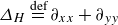 $\varDelta _H\overset {{\text{def}}}{=} \partial _{xx}+\partial _{yy}$
and
$\varDelta _H\overset {{\text{def}}}{=} \partial _{xx}+\partial _{yy}$
and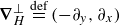 $\boldsymbol{\nabla} _H^\perp \overset {{\text{def}}}{=} (-\partial _y, \partial _x )$
. When
$\boldsymbol{\nabla} _H^\perp \overset {{\text{def}}}{=} (-\partial _y, \partial _x )$
. When $\alpha =0$
, since
$\alpha =0$
, since $\mathcal{S}=\mathcal{S}^{-1}=I$
, this correctly reduces to the projection operator in the QG,
$\mathcal{S}=\mathcal{S}^{-1}=I$
, this correctly reduces to the projection operator in the QG, $\alpha =0$
case in Whitehead & Wingate (Reference Whitehead and Wingate2014).
$\alpha =0$
case in Whitehead & Wingate (Reference Whitehead and Wingate2014).
The (slow) QG- $\alpha$
dynamics are (see Appendix A.3)
$\alpha$
dynamics are (see Appendix A.3)
 \begin{equation} \frac {D^{H,\alpha }}{Dt}\left (\varDelta _H\mathcal{S} \phi + F^2 \mathcal{S}^{-1}\frac {\partial ^2}{\partial z^2}\phi \right )=0, \end{equation}
where $( {D^{H,\alpha }}/{Dt}\overset {{\text{def}}}){=} ( {\partial }/{\partial t} )+ \boldsymbol{u}_H\boldsymbol{\cdot }\boldsymbol{\nabla} _H$
and
$( {D^{H,\alpha }}/{Dt}\overset {{\text{def}}}){=} ( {\partial }/{\partial t} )+ \boldsymbol{u}_H\boldsymbol{\cdot }\boldsymbol{\nabla} _H$
and $\phi$
denotes the potential (here, the modified pressure), so that the vertical vorticity
$\phi$
denotes the potential (here, the modified pressure), so that the vertical vorticity $\omega _3= \mathcal{S} \varDelta _H \phi$
. By using the commutative properties of
$\omega _3= \mathcal{S} \varDelta _H \phi$
. By using the commutative properties of $\mathcal{S}$
, we can see that analogously to the
$\mathcal{S}$
, we can see that analogously to the $\alpha =0$
case, the potential vorticity is simply the
$\alpha =0$
case, the potential vorticity is simply the $\Delta _{{\textit{QG}}_\alpha }$
operator applied to the potential
$\Delta _{{\textit{QG}}_\alpha }$
operator applied to the potential $\phi$
. We can also rewrite (3.9) as
$\phi$
. We can also rewrite (3.9) as
 \begin{equation} \frac {D^{H,\alpha }}{Dt}\left (\omega _3 - F \mathcal{S}^{-1}\frac {\partial }{\partial z}\rho \right )=0, \end{equation}
which is very similar to the PV conservation equation in the $\alpha =0$
case:
$\alpha =0$
case:
 \begin{equation} \frac {D^H}{Dt}\left (\omega _3 - F \frac {\partial }{\partial z}\rho \right )=0, \end{equation}
where the vertical vorticity reduces to $\omega _3 =\varDelta _H p$
as usual, since
$\omega _3 =\varDelta _H p$
as usual, since $\mathcal{S}=I$
in the
$\mathcal{S}=I$
in the $\alpha =0$
case. The key differences between (the slow portion of) QG-
$\alpha =0$
case. The key differences between (the slow portion of) QG- $\alpha$
, (3.10), and the usual QG, (3.11), are that in QG-
$\alpha$
, (3.10), and the usual QG, (3.11), are that in QG- $\alpha$
, the density is now filtered, the vorticity has a different relationship to the (modified) pressure, now involving the Helmholtz operator, and the material derivative is with respect to the transport velocity. Thus, the dominant, slow QG-
$\alpha$
, the density is now filtered, the vorticity has a different relationship to the (modified) pressure, now involving the Helmholtz operator, and the material derivative is with respect to the transport velocity. Thus, the dominant, slow QG- $\alpha$
dynamics are regularised compared with the dominant, slow QG
$\alpha$
dynamics are regularised compared with the dominant, slow QG $(\alpha =0)$
dynamics (figure 1): an expected outcome given that LANS-
$(\alpha =0)$
dynamics (figure 1): an expected outcome given that LANS- $\alpha$
is a regularised model.
$\alpha$
is a regularised model.
3.4. Fast limiting dynamics and modifications of triad interactions by
$\alpha$

While $\alpha$
regularises the dynamics, we find that it alters the balance between the slow and fast dynamics, amplifying the role of the fast dynamics. To show this, we analyse the triad interactions within the LANS-
$\alpha$
regularises the dynamics, we find that it alters the balance between the slow and fast dynamics, amplifying the role of the fast dynamics. To show this, we analyse the triad interactions within the LANS- $\alpha$
equations and compare with those of the unregularised equations. Although LANS-
$\alpha$
equations and compare with those of the unregularised equations. Although LANS- $\alpha$
is motivated by Lagrangian averaging, in this paper we interpret
$\alpha$
is motivated by Lagrangian averaging, in this paper we interpret $\alpha$
primarily as a scale-selective regularisation: it modifies dynamics at wavelengths comparable to, or smaller than,
$\alpha$
primarily as a scale-selective regularisation: it modifies dynamics at wavelengths comparable to, or smaller than, $\alpha$
, while leaving longer-wave motions essentially unchanged in the resolved fields. A useful parallel is Bretherton’s (Reference Bretherton1969) calculation of the mean flow induced by a short internal-gravity wave packet, where averaging over the fast oscillatory wave phase removes the short-wave oscillations but, in the two-dimensional case, leaves a quasi-hydrostatic radiation field of long internal waves; to leading order, the packet propagates with the group velocity while the total horizontal pseudo-momentum associated with the packet is conserved. Hence, averaging over fast wave scales need not remove all wave motion; in the
$\alpha$
, while leaving longer-wave motions essentially unchanged in the resolved fields. A useful parallel is Bretherton’s (Reference Bretherton1969) calculation of the mean flow induced by a short internal-gravity wave packet, where averaging over the fast oscillatory wave phase removes the short-wave oscillations but, in the two-dimensional case, leaves a quasi-hydrostatic radiation field of long internal waves; to leading order, the packet propagates with the group velocity while the total horizontal pseudo-momentum associated with the packet is conserved. Hence, averaging over fast wave scales need not remove all wave motion; in the $\alpha$
-regularised equations, long-wave inertia–gravity modes likewise remain, so it is natural to consider how
$\alpha$
-regularised equations, long-wave inertia–gravity modes likewise remain, so it is natural to consider how $\alpha$
shifts their dispersion relations and the associated resonance conditions.
$\alpha$
shifts their dispersion relations and the associated resonance conditions.
The dispersion relations for the modes associated with the fast QG- $\alpha$
limit are found by seeking eigenfunctions of the fast operator
$\alpha$
limit are found by seeking eigenfunctions of the fast operator $\mathcal{L}_F$
of the form
$\mathcal{L}_F$
of the form
 \begin{equation} \boldsymbol{w} = \exp (i\boldsymbol{k}\boldsymbol{\cdot }\boldsymbol{x} - i\omega (\boldsymbol{k})t)\boldsymbol{r}, \end{equation}
where $\boldsymbol{r}$
is an associated eigenvector,
$\boldsymbol{r}$
is an associated eigenvector, $\omega (\boldsymbol{k})$
is an associated eigenfrequency and
$\omega (\boldsymbol{k})$
is an associated eigenfrequency and $\boldsymbol{k}=(k_1,k_2,k_3)$
is a wavenumber. In this context,
$\boldsymbol{k}=(k_1,k_2,k_3)$
is a wavenumber. In this context, $\omega (\boldsymbol{k})$
will be either zero or the classic inertia–gravity wave dispersion relation. We also denote
$\omega (\boldsymbol{k})$
will be either zero or the classic inertia–gravity wave dispersion relation. We also denote
 \begin{equation} |\boldsymbol{k}|\overset {{\text{def}}}{=} \left(k_1^2+k_2^2+k_3^2\right)^{{1}/{2}} \quad \text{and} \quad |\boldsymbol{k}_H|\overset {{\text{def}}}{=}\left(k_1^2+k_2^2\right)^{ {1}/{2}}. \end{equation}
Analytic formulas for the eigenfrequencies are required to characterise all possible three-wave resonances. In the usual fast QG limit, the eigenfrequencies are given by (Embid & Majda Reference Embid and Majda1998)
 \begin{equation} \omega ^{(0)}(\boldsymbol{k})=0 \quad \text{(double root)} \quad \text{ and } \quad \omega ^{(\pm 1)}(\boldsymbol{k}) = \pm \frac {\left(|\boldsymbol{k}_H|^2+F^2k_3^2\right)^{ {1}/{2}}}{|\boldsymbol{k}|}. \end{equation}
Physically, the zero-frequency (slow) modes are zero-frequency Rossby waves, while the modes with frequency $\omega ^{(\pm 1)}$
are (dispersive) inertia–gravity waves. The parameter
$\omega ^{(\pm 1)}$
are (dispersive) inertia–gravity waves. The parameter $F=f/N$
appears in the dispersion relation (3.14) and sets the relative importance of vertical versus horizontal structure. For instance, when stratification is stronger than rotation (
$F=f/N$
appears in the dispersion relation (3.14) and sets the relative importance of vertical versus horizontal structure. For instance, when stratification is stronger than rotation ( $N\gt f)$
, the impact of vertical variations on the inertia–gravity wave frequency is reduced.
$N\gt f)$
, the impact of vertical variations on the inertia–gravity wave frequency is reduced.
Summary of the four types of relevant resonant and near-resonant interactions. Note that Fourier coefficients for fast–fast–slow interactions are zero (Embid & Majda Reference Embid and Majda1998), which does not change when $\alpha \neq 0$
. For wavenumbers
$\alpha \neq 0$
. For wavenumbers $\boldsymbol{k}+\boldsymbol{p}=\boldsymbol{q}$
, the eigenfrequency condition for (all but slow–slow–slow) resonances to occur changes with the parameter
$\boldsymbol{k}+\boldsymbol{p}=\boldsymbol{q}$
, the eigenfrequency condition for (all but slow–slow–slow) resonances to occur changes with the parameter $\alpha$
. The resonance types are listed in order of their frequency and importance for energy transfer in the case
$\alpha$
. The resonance types are listed in order of their frequency and importance for energy transfer in the case $\alpha =0$
. Slow–slow–slow interactions are the most numerous but are unaffected by
$\alpha =0$
. Slow–slow–slow interactions are the most numerous but are unaffected by $\alpha$
. Fast–fast–fast interactions have been less considered because they occur only sparsely, though this changes when
$\alpha$
. Fast–fast–fast interactions have been less considered because they occur only sparsely, though this changes when $\alpha \neq 0$
. For more details, see Appendix B.2.
$\alpha \neq 0$
. For more details, see Appendix B.2.

Table 1. Long description
Table 1 has four columns: resonance type, α = 0 condition, α ≠ 0 condition, and role in energy evolution. The four rows list slow-slow-slow, slow-fast-fast, fast-fast-fast, and slow-slow-fast interactions. The table shows that slow-slow-slow interactions occur for all wavenumbers and are unaffected by α. Slow-fast-fast and fast-fast-fast resonance conditions change when α is nonzero, because the dispersion relation is modified. Exact slow-slow-fast resonances remain absent, although near-resonance locations may be distorted.
In the fast QG- $\alpha$
limit, the eigenfrequencies are modified by the non-dimensional Helmholtz operator in spectral space,
$\alpha$
limit, the eigenfrequencies are modified by the non-dimensional Helmholtz operator in spectral space, $(1+L_\alpha |\boldsymbol{k}|^2)$
, where
$(1+L_\alpha |\boldsymbol{k}|^2)$
, where $L_\alpha =\alpha ^2/L^2$
is the non-dimensionalised version of
$L_\alpha =\alpha ^2/L^2$
is the non-dimensionalised version of $\alpha ^2$
. The eigenfrequencies when
$\alpha ^2$
. The eigenfrequencies when $\alpha \neq 0$
(
$\alpha \neq 0$
( $L_\alpha \neq 0$
) are given by
$L_\alpha \neq 0$
) are given by
 \begin{align} \omega ^{(0)}(\boldsymbol{k})=0 \quad \text{(double root)} \quad \text{ and } \quad \omega ^{(\pm 1)}(\boldsymbol{k}) = \pm \frac {\left(\left(1+L_\alpha |\boldsymbol{k}|^2\right)|\boldsymbol{k}_H|^2+F^2k_3^2\right)^{ {1}/{2}}}{\left(1+L_\alpha |\boldsymbol{k}|^2\right)|\boldsymbol{k}|}. \end{align}
Smaller $L_\alpha$
corresponds to
$L_\alpha$
corresponds to $\alpha$
-regularised dynamics that is closer to the unregularised dynamics. In the limit
$\alpha$
-regularised dynamics that is closer to the unregularised dynamics. In the limit $L_\alpha =0$
, the regularisation vanishes; (3.15) then reduces to (3.14).
$L_\alpha =0$
, the regularisation vanishes; (3.15) then reduces to (3.14).
The set of resonant triads is described by
 \begin{equation} R_{\beta , \boldsymbol{q}}^\alpha \overset {{\text{def}}}{=} \left\{\big(\boldsymbol{k}, \boldsymbol{p}, \beta ', \beta ''\big)\;|\; \boldsymbol{k}+\boldsymbol{p}=\boldsymbol{q}, \; \omega ^{(\beta ')}(\boldsymbol{k})+\omega ^{(\beta '')}(\boldsymbol{p}) = \omega ^{(\beta )}(\boldsymbol{q})\right\}\!, \end{equation}
where the superscript $\alpha$
emphasises that the set of possible interactions now depends on
$\alpha$
emphasises that the set of possible interactions now depends on $\alpha$
due to (3.15). The relevant classes of triads are described in table 1. Of these, we consider the slow–fast–fast and fast–fast–fast triads, as the set of possible slow–slow–slow resonances does not change with
$\alpha$
due to (3.15). The relevant classes of triads are described in table 1. Of these, we consider the slow–fast–fast and fast–fast–fast triads, as the set of possible slow–slow–slow resonances does not change with $\alpha$
and there are no slow–slow–fast resonances or near-resonances when both
$\alpha$
and there are no slow–slow–fast resonances or near-resonances when both $\alpha =0$
and
$\alpha =0$
and $\alpha \neq 0$
(for conservative tolerance levels, see supplementary material, figures S1–S3 and S7, available at https://doi.org/10.1017/jfm.2026.11720.).
$\alpha \neq 0$
(for conservative tolerance levels, see supplementary material, figures S1–S3 and S7, available at https://doi.org/10.1017/jfm.2026.11720.).
Slow–fast–fast interactions, when $F\approx 1$
(
$F\approx 1$
( ${\textit{Bu}}\approx 1$
), have been seen to result in a rapid downscale energy transfer, and have been described as catalytic interactions responsible for the emergence of a geostrophically adjusted state (Bartello Reference Bartello1995). When the eigenfrequencies are given by (3.14), the condition for the pair of wavenumbers
${\textit{Bu}}\approx 1$
), have been seen to result in a rapid downscale energy transfer, and have been described as catalytic interactions responsible for the emergence of a geostrophically adjusted state (Bartello Reference Bartello1995). When the eigenfrequencies are given by (3.14), the condition for the pair of wavenumbers $\boldsymbol{k}$
and
$\boldsymbol{k}$
and $\boldsymbol{p}$
, with
$\boldsymbol{p}$
, with $\boldsymbol{k}+\boldsymbol{p}=\boldsymbol{q}$
, to be an element of
$\boldsymbol{k}+\boldsymbol{p}=\boldsymbol{q}$
, to be an element of $R_{\beta ,\boldsymbol{q}}^0$
(with
$R_{\beta ,\boldsymbol{q}}^0$
(with $\beta '=\pm 1, \beta ''=0, \beta =\pm 1$
), as defined in (3.16), is
$\beta '=\pm 1, \beta ''=0, \beta =\pm 1$
), as defined in (3.16), is
 \begin{equation} \pm \frac {\left(|\boldsymbol{k}_H|^2+F^2k_3^2\right)^{{1}/{2}}}{|\boldsymbol{k}|} = \pm \frac {\left(|\boldsymbol{q}_H|^2+F^2q_3^2\right)^{{1}/{2}}}{|\boldsymbol{q}|}, \end{equation}
or similarly with $\boldsymbol{p}$
in place of
$\boldsymbol{p}$
in place of $\boldsymbol{k}$
, interchanging the roles of
$\boldsymbol{k}$
, interchanging the roles of $\beta '$
and
$\beta '$
and $\beta ''$
. The condition (3.17) produces a resonance for any
$\beta ''$
. The condition (3.17) produces a resonance for any $\boldsymbol{k}, \boldsymbol{p}, \boldsymbol{q}$
when
$\boldsymbol{k}, \boldsymbol{p}, \boldsymbol{q}$
when $F=1$
or a near-resonance when
$F=1$
or a near-resonance when $F=O(1)$
. When the eigenfrequencies are instead given by (3.15), the condition is
$F=O(1)$
. When the eigenfrequencies are instead given by (3.15), the condition is
 \begin{equation} \pm \frac {\left(\left(1+L_\alpha |\boldsymbol{k}|^2\right)|\boldsymbol{k}_H|^2+F^2 k_3^2\right)^{{1}/{2}}}{\left(1+L_\alpha |\boldsymbol{k}|^2\right)|\boldsymbol{k}|} = \pm \frac {\left(\left(1+L_\alpha |\boldsymbol{q}|^2\right)|\boldsymbol{q}_H|^2+F^2 q_3^2\right)^{{1}/{2}}}{\left(1+L_\alpha |\boldsymbol{q}|^2\right)|\boldsymbol{q}|}, \end{equation}
or similarly with $\boldsymbol{p}$
upon interchanging the roles of
$\boldsymbol{p}$
upon interchanging the roles of $\beta '$
and
$\beta '$
and $\beta ''$
.
$\beta ''$
.
Due to the additional nonlinearity of (3.18) as compared with (3.17), it is challenging to reason analytically exactly how the number and distribution of the elements of $R_{\beta ,\boldsymbol{q}}^\alpha$
change with
$R_{\beta ,\boldsymbol{q}}^\alpha$
change with $\alpha$
(or
$\alpha$
(or $L_\alpha$
), but it is possible to do so numerically. Our results show that for
$L_\alpha$
), but it is possible to do so numerically. Our results show that for $F=1$
(
$F=1$
( ${\textit{Bu}}=1$
), the introduction of a non-zero
${\textit{Bu}}=1$
), the introduction of a non-zero $\alpha$
drastically curtails the number of slow–fast–fast resonant triads, including the cross-scale interactions responsible for transferring energy between large-scale and small-scale dynamics (figure 2). This reduction disrupts the primary channel for downscale energy transfer. Further increasing
$\alpha$
drastically curtails the number of slow–fast–fast resonant triads, including the cross-scale interactions responsible for transferring energy between large-scale and small-scale dynamics (figure 2). This reduction disrupts the primary channel for downscale energy transfer. Further increasing $L_\alpha$
leads to an increase in the number of resonances, though it does not return to the number when
$L_\alpha$
leads to an increase in the number of resonances, though it does not return to the number when $L_\alpha =0$
for reasonable values of
$L_\alpha =0$
for reasonable values of $L_\alpha$
(given that in modelling studies, typically
$L_\alpha$
(given that in modelling studies, typically $\alpha$
is only a few grid points in length, i.e.
$\alpha$
is only a few grid points in length, i.e. $\alpha = 2\Delta x$
). For the regimes in which this energy pathway is already less active,
$\alpha = 2\Delta x$
). For the regimes in which this energy pathway is already less active, $F=1/2$
(
$F=1/2$
( ${\textit{Bu}}=4$
) and
${\textit{Bu}}=4$
) and $F=2$
(
$F=2$
( ${\textit{Bu}}=1/4$
), the introduction of non-zero
${\textit{Bu}}=1/4$
), the introduction of non-zero $\alpha$
has a different effect, only increasing the number of resonances and thus altering rather than shutting down energy exchange via slow–fast–fast resonances.
$\alpha$
has a different effect, only increasing the number of resonances and thus altering rather than shutting down energy exchange via slow–fast–fast resonances.
Regularisation by $\alpha$
(
$\alpha$
( $L_\alpha =\alpha ^2/L^2$
) reshapes the landscape of resonant interactions, superseding the ratio
$L_\alpha =\alpha ^2/L^2$
) reshapes the landscape of resonant interactions, superseding the ratio $F=f/N$
(thus also the Burger number,
$F=f/N$
(thus also the Burger number, ${\textit{Bu}}=N^2/f^2$
) as the dominant parameter determining the relative amounts of different resonances, once
${\textit{Bu}}=N^2/f^2$
) as the dominant parameter determining the relative amounts of different resonances, once $L_\alpha$
is sufficiently large. As
$L_\alpha$
is sufficiently large. As $L_\alpha$
increases, the counts of both slow–fast–fast and fast–fast–fast resonant and near-resonant interactions converge to values largely independent of
$L_\alpha$
increases, the counts of both slow–fast–fast and fast–fast–fast resonant and near-resonant interactions converge to values largely independent of $F$
. All counts were computed on a grid of
$F$
. All counts were computed on a grid of $256^3$
using a tolerance of
$256^3$
using a tolerance of $10^{-5}$
for numerically checking the resonance conditions (see supplementary materials for the robustness across different tolerance levels). For each line style (fixed
$10^{-5}$
for numerically checking the resonance conditions (see supplementary materials for the robustness across different tolerance levels). For each line style (fixed $F$
), both slow–fast–fast (black) and fast–fast–fast (grey) triad counts are computed using that same
$F$
), both slow–fast–fast (black) and fast–fast–fast (grey) triad counts are computed using that same $F$
in the dispersion relation for all three modes. The slow–fast–fast curves for different
$F$
in the dispersion relation for all three modes. The slow–fast–fast curves for different $F$
are indistinguishable, given sufficiently large
$F$
are indistinguishable, given sufficiently large $L_\alpha$
, on the logarithmic
$L_\alpha$
, on the logarithmic $y$
axis and appear as a single curve. The fast–fast–fast curves are similarly close, for all
$y$
axis and appear as a single curve. The fast–fast–fast curves are similarly close, for all $L_\alpha$
, and appear as a single (overlapping) curve. Given the large number of wavenumbers associated with the
$L_\alpha$
, and appear as a single (overlapping) curve. Given the large number of wavenumbers associated with the $256^3$
grid, it was possible for the resonance conditions to be satisfied a large number of times (up to trillions, as shown here). To focus on general three-dimensional interactions, triads involving purely horizontal or purely vertical wavenumbers were excluded from the count.
$256^3$
grid, it was possible for the resonance conditions to be satisfied a large number of times (up to trillions, as shown here). To focus on general three-dimensional interactions, triads involving purely horizontal or purely vertical wavenumbers were excluded from the count.

Figure 2. Long description
Figure 2 is a line plot with L_α on the horizontal axis and number of interactions on the logarithmic vertical axis. Black markers and curves represent slow-fast-fast triads, while grey markers and curves represent fast-fast-fast triads. Different line styles represent F = 1/2, F = 1, and F = 2. At L_α = 0, the slow-fast-fast counts depend strongly on F, while fast-fast-fast counts are absent or much smaller. As L_α increases, the fast-fast-fast counts rise sharply, and the counts for both interaction classes become much less dependent on F.
A detailed view of the change in the number of resonant interactions for small values of $L_\alpha$
, for three values of the rotation-to-stratification ratio
$L_\alpha$
, for three values of the rotation-to-stratification ratio $F=f/N$
(
$F=f/N$
( $F=1/2,1,2$
), shows that the number of fast–fast–fast triads appears to grow continuously with
$F=1/2,1,2$
), shows that the number of fast–fast–fast triads appears to grow continuously with $L_\alpha$
, rather than emerging in a discontinuous jump. Concurrently, the count of slow–fast–fast interactions exhibits an inflection point with
$L_\alpha$
, rather than emerging in a discontinuous jump. Concurrently, the count of slow–fast–fast interactions exhibits an inflection point with $L_\alpha$
. These counts are computed in the same manner as those in figure 2, but with respect to a range of smaller
$L_\alpha$
. These counts are computed in the same manner as those in figure 2, but with respect to a range of smaller $L_\alpha$
values.
$L_\alpha$
values.

Figure 3. Long description
Figure 3 contains three narrow plots arranged horizontally and labelled F = 1/2, F = 1, and F = 2. Each panel has L_α on the horizontal axis and number of interactions on the logarithmic vertical axis. Black curves show slow-fast-fast counts, and grey curves show fast-fast-fast counts. The grey fast-fast-fast curves rise from zero or near zero as L_α increases. The black slow-fast-fast curves bend downward and then upward, showing an inflection in the count at small L_α values.
Fast–fast–fast exact resonant interactions do not occur when $1/2\leq F\leq 2$
in the
$1/2\leq F\leq 2$
in the $\alpha =0$
case, and resonant and near-resonant interactions occur only rarely otherwise. The condition is
$\alpha =0$
case, and resonant and near-resonant interactions occur only rarely otherwise. The condition is
 \begin{equation} \pm \frac {\left(|\boldsymbol{k}_H|^2+F^2k_3^2\right)^{ {1}/{2}}}{|\boldsymbol{k}|} \pm \frac {\left(|\boldsymbol{p}_H|^2+F^2p_3^2\right)^{ {1}/{2}}}{|\boldsymbol{p}|}= \pm \frac {\left(|\boldsymbol{q}_H|^2+F^2q_3^2\right)^{ {1}/{2}}}{|\boldsymbol{q}|}. \end{equation}
When $\alpha \neq 0$
, (3.19) becomes instead
$\alpha \neq 0$
, (3.19) becomes instead
 \begin{align} \pm \frac {\left(\left(1+L_\alpha |\boldsymbol{k}|^2\right)|\boldsymbol{k}_H|^2+F^2 k_3^2\right)^{ {1}/{2}}}{\left(1+L_\alpha |\boldsymbol{k}|^2\right)|\boldsymbol{k}|} &\pm \frac {\left(\left(1+L_\alpha |\boldsymbol{p}|^2\right)|\boldsymbol{p}_H|^2+F^2 p_3^2\right)^{ {1}/{2}}}{\left(1+L_\alpha |\boldsymbol{p}|^2\right)|\boldsymbol{p}|} \notag\\&= \pm \frac {\left(\left(1+L_\alpha |\boldsymbol{q}|^2\right)|\boldsymbol{q}_H|^2+F^2 q_3^2\right)^{ {1}/{2}}}{\left(1+L_\alpha |\boldsymbol{q}|^2\right)|\boldsymbol{q}|}. \end{align}
The new nonlinearity and dependence on wavenumber in (3.20) allows the number of fast–fast–fast resonances to significantly increase, even in cases where it is usually zero without $\alpha$
-regularisation. When
$\alpha$
-regularisation. When $\alpha \neq 0$
, the number of fast–fast–fast resonant interactions becomes comparable to the number of slow–fast–fast resonant interactions (figure 2) for every value of
$\alpha \neq 0$
, the number of fast–fast–fast resonant interactions becomes comparable to the number of slow–fast–fast resonant interactions (figure 2) for every value of $F$
(
$F$
( $F={1}/{2},1,2$
). This stands in stark contrast to the usual fast QG limit, where fast–fast–fast triads are typically sparse or non-existent. The emergence of a large number of fast–fast–fast resonances allows energy to be efficiently exchanged and redistributed purely among the fast modes, independent of the slow vortical flow. A detailed view of this emergence (figure 3) confirms that the number of fast–fast–fast triads appears to grow continuously from
$F={1}/{2},1,2$
). This stands in stark contrast to the usual fast QG limit, where fast–fast–fast triads are typically sparse or non-existent. The emergence of a large number of fast–fast–fast resonances allows energy to be efficiently exchanged and redistributed purely among the fast modes, independent of the slow vortical flow. A detailed view of this emergence (figure 3) confirms that the number of fast–fast–fast triads appears to grow continuously from $L_\alpha =0$
rather than spiking discontinuously; this is especially evident in the
$L_\alpha =0$
rather than spiking discontinuously; this is especially evident in the $F=1/2$
(
$F=1/2$
( ${\textit{Bu}}=4$
) and
${\textit{Bu}}=4$
) and $F=2$
(
$F=2$
( ${\textit{Bu}}=1/4$
) plots.
${\textit{Bu}}=1/4$
) plots.
Perhaps most significantly, as $\alpha$
becomes sufficiently large, the numbers of both slow–fast–fast triads and fast–fast–fast triads converge to values largely independent of the rotation-to-stratification ratio
$\alpha$
becomes sufficiently large, the numbers of both slow–fast–fast triads and fast–fast–fast triads converge to values largely independent of the rotation-to-stratification ratio $F$
, indicating that
$F$
, indicating that $\alpha$
supersedes
$\alpha$
supersedes $F$
as the dominant parameter shaping the potential for resonant interactions. The overall effect of
$F$
as the dominant parameter shaping the potential for resonant interactions. The overall effect of $\alpha$
on the fast dynamics is not to simply regularise but to restructure the energy pathways.
$\alpha$
on the fast dynamics is not to simply regularise but to restructure the energy pathways.
4. Numerical simulations
4.1. Description of the numerical method
For all numerical experiments, we use Dedalus, a pseudo-spectral solver in Python (Burns et al. Reference Burns, Vasil, Oishi, Lecoanet and Brown2020). The non-dimensional LANS- $\alpha$
equations (2.8a
–
c
) are solved within the triply periodic domain
$\alpha$
equations (2.8a
–
c
) are solved within the triply periodic domain $[0,1]^3$
, discretised on a uniform grid of
$[0,1]^3$
, discretised on a uniform grid of $N^3=256^3$
points with a
$N^3=256^3$
points with a $3/2$
dealiasing rule. The system is initialised from a state of rest. For time stepping, we employ an explicit second-order, two-stage Runge–Kutta scheme (RK222). This scheme was selected for computational efficiency and validation runs confirmed its results were comparable to those from the third-order, four-stage scheme (RK443). The time step is adjusted dynamically by a Courant–Friedrichs–Lewy condition determined by the maximum total frequency corresponding to the unregularised velocity
$3/2$
dealiasing rule. The system is initialised from a state of rest. For time stepping, we employ an explicit second-order, two-stage Runge–Kutta scheme (RK222). This scheme was selected for computational efficiency and validation runs confirmed its results were comparable to those from the third-order, four-stage scheme (RK443). The time step is adjusted dynamically by a Courant–Friedrichs–Lewy condition determined by the maximum total frequency corresponding to the unregularised velocity $\boldsymbol{v}$
, across the grid (see Burns et al. (Reference Burns, Vasil, Oishi, Lecoanet and Brown2020) for more details).
$\boldsymbol{v}$
, across the grid (see Burns et al. (Reference Burns, Vasil, Oishi, Lecoanet and Brown2020) for more details).
The physical set-up of our experiments is similar to that of Smith & Waleffe (Reference Smith and Waleffe2002). Energy is injected by selecting a divergence-free forcing $\mathcal{F}$
in the momentum equation whose spectral shape is inspired by Smith & Waleffe (Reference Smith and Waleffe2002), but which is constant in time (as in Wingate et al. Reference Wingate, Embid, Holmes-Cerfon and Taylor2011). An isotropic amplitude distribution is prescribed via the scalar spectrum
$\mathcal{F}$
in the momentum equation whose spectral shape is inspired by Smith & Waleffe (Reference Smith and Waleffe2002), but which is constant in time (as in Wingate et al. Reference Wingate, Embid, Holmes-Cerfon and Taylor2011). An isotropic amplitude distribution is prescribed via the scalar spectrum $f(|\boldsymbol{k}|)$
, which is a Gaussian in wavenumber space, centred at the forcing wavenumber
$f(|\boldsymbol{k}|)$
, which is a Gaussian in wavenumber space, centred at the forcing wavenumber $k_f$
:
$k_f$
:
 \begin{equation} f(|\boldsymbol{k}|) = \frac {\epsilon _f}{(2\pi )^{{1}/{2}}s}\exp \left (\frac {-(|\boldsymbol{k}| -k_f)^2}{2s^2}\right )\!. \end{equation}
Specifically, the coefficients are normalised so that the shell-wise mean-square amplitude follows $f(|\boldsymbol{k}|)$
, so
$f(|\boldsymbol{k}|)$
, so $\epsilon _f$
is referred to as the forcing-amplitude parameter (it is not generally a realised energy injection rate, except under specific scaling choices). The forcing-amplitude parameter is
$\epsilon _f$
is referred to as the forcing-amplitude parameter (it is not generally a realised energy injection rate, except under specific scaling choices). The forcing-amplitude parameter is $\epsilon _f=1$
and the standard deviation is
$\epsilon _f=1$
and the standard deviation is $s=1$
for all simulations. Since we are interested in the QG limit, we use low wavenumber forcing,
$s=1$
for all simulations. Since we are interested in the QG limit, we use low wavenumber forcing, $k_f=3(2\pi )$
. The choice of a time-independent forcing is motivated primarily by the need for grid-scale convergence studies. One issue is that the LANS-
$k_f=3(2\pi )$
. The choice of a time-independent forcing is motivated primarily by the need for grid-scale convergence studies. One issue is that the LANS- $\alpha$
model presents known stability challenges, and verifying grid-scale convergence at each value of
$\alpha$
model presents known stability challenges, and verifying grid-scale convergence at each value of $L_\alpha$
is essential. Another issue is that
$L_\alpha$
is essential. Another issue is that $\alpha$
itself modifies the effective dissipation range (Chen et al. Reference Chen, Holm, Margolin and Zhang1999), so that the resolution requirements change with
$\alpha$
itself modifies the effective dissipation range (Chen et al. Reference Chen, Holm, Margolin and Zhang1999), so that the resolution requirements change with $L_\alpha$
. Together, these make convergence verification both essential and non-trivial. A stochastic-in-time forcing as in Smith & Waleffe (Reference Smith and Waleffe2002) and Sukhatme & Smith (Reference Sukhatme and Smith2008) compounds both difficulties, as random realisations can push the model outside its region of stability unpredictably. These considerations lead us to choose forcing and viscosity for the study in this paper that are fixed in time. This forcing defines a characteristic time scale:
$L_\alpha$
. Together, these make convergence verification both essential and non-trivial. A stochastic-in-time forcing as in Smith & Waleffe (Reference Smith and Waleffe2002) and Sukhatme & Smith (Reference Sukhatme and Smith2008) compounds both difficulties, as random realisations can push the model outside its region of stability unpredictably. These considerations lead us to choose forcing and viscosity for the study in this paper that are fixed in time. This forcing defines a characteristic time scale:
 \begin{equation} \tau = \left(\epsilon _f k_f^2\right)^{-{1}/{3}}. \end{equation}
All simulations are integrated to a final non-dimensional time of $t_f=1$
, corresponding to approximately
$t_f=1$
, corresponding to approximately $7\tau$
. In the simulations, we are particularly interested in whether
$7\tau$
. In the simulations, we are particularly interested in whether $\alpha$
modifies the first crossover time (as in Sukhatme & Smith Reference Sukhatme and Smith2008), which is the first time at which the energy in the geostrophic (or vortical) modes exceeds that in the wave modes. Comparing the crossover times for different values of
$\alpha$
modifies the first crossover time (as in Sukhatme & Smith Reference Sukhatme and Smith2008), which is the first time at which the energy in the geostrophic (or vortical) modes exceeds that in the wave modes. Comparing the crossover times for different values of $\alpha$
, all else equal, provides a measure of how rapidly the partition of energy reorganises and thus how
$\alpha$
, all else equal, provides a measure of how rapidly the partition of energy reorganises and thus how $\alpha$
modifies the relative effectiveness of wave-sustaining pathways. This will also show how the
$\alpha$
modifies the relative effectiveness of wave-sustaining pathways. This will also show how the $\alpha$
-modification of the triad interactions (§ 3.4) manifests in the energy evolution. We choose the final time of
$\alpha$
-modification of the triad interactions (§ 3.4) manifests in the energy evolution. We choose the final time of $t_f=1$
for the simulations in accordance with this goal of observing the initial development of the turbulent flow involving the transfer of energy between vortical and wave modes.
$t_f=1$
for the simulations in accordance with this goal of observing the initial development of the turbulent flow involving the transfer of energy between vortical and wave modes.
In (2.8a
), we use a hyperviscosity and set $\mathcal{D}_\nu \boldsymbol{v} = \nu (-1)^{n+1}\boldsymbol{\nabla} ^{2n} \boldsymbol{v}$
and
$\mathcal{D}_\nu \boldsymbol{v} = \nu (-1)^{n+1}\boldsymbol{\nabla} ^{2n} \boldsymbol{v}$
and $\mathcal{D}_\kappa \rho = \kappa (-1)^{n+1} \boldsymbol{\nabla} ^{2n} \rho$
with
$\mathcal{D}_\kappa \rho = \kappa (-1)^{n+1} \boldsymbol{\nabla} ^{2n} \rho$
with $n=8$
, as in Smith & Waleffe (Reference Smith and Waleffe2002), except the coefficients
$n=8$
, as in Smith & Waleffe (Reference Smith and Waleffe2002), except the coefficients $\nu$
and
$\nu$
and $\kappa$
are constant in time and defined based on the dealiased grid cutoff wavenumber, to allow for more direct comparisons across simulations of different grid sizes.
$\kappa$
are constant in time and defined based on the dealiased grid cutoff wavenumber, to allow for more direct comparisons across simulations of different grid sizes.
We investigate the system’s behaviour for three values of $F$
: 1 (equally strong rotation and stratification), 2 (stronger rotation) and 1/2 (stronger stratification), achieved by setting
$F$
: 1 (equally strong rotation and stratification), 2 (stronger rotation) and 1/2 (stronger stratification), achieved by setting $(Ro, Fr) = (0.1, 0.1)$
,
$(Ro, Fr) = (0.1, 0.1)$
, $(0.1, 0.2)$
and
$(0.1, 0.2)$
and $(0.2, 0.1)$
, respectively. In all cases, both
$(0.2, 0.1)$
, respectively. In all cases, both $Ro$
and
$Ro$
and ${\textit{Fr}}$
are small in order to reflect the QG limit. For each
${\textit{Fr}}$
are small in order to reflect the QG limit. For each $F$
, we systematically vary the non-dimensional regularisation parameter across five values:
$F$
, we systematically vary the non-dimensional regularisation parameter across five values: $L_\alpha = 0, 0.01, 0.1, 0.15, 0.2$
.
$L_\alpha = 0, 0.01, 0.1, 0.15, 0.2$
.
A representative snapshot from the simulations is shown in figure 4, which also illustrates how the distinction between the velocities $\boldsymbol{v}$
and
$\boldsymbol{v}$
and $\boldsymbol{u}$
manifests under LANS-
$\boldsymbol{u}$
manifests under LANS- $\alpha$
regularisation.
$\alpha$
regularisation.
Representative snapshots of horizontal velocity fields from the LANS- $\alpha$
simulations. Panels show the first horizontal component over a horizontal plane at
$\alpha$
simulations. Panels show the first horizontal component over a horizontal plane at $z=0.5$
and
$z=0.5$
and $t=0.5$
: (a) the unregularised
$t=0.5$
: (a) the unregularised $x$
-velocity
$x$
-velocity $v_1$
for
$v_1$
for $L_\alpha =0$
, (b) the unregularised
$L_\alpha =0$
, (b) the unregularised $x$
-velocity
$x$
-velocity $v_1$
for
$v_1$
for $L_\alpha =0.1$
and (c) the associated regularised
$L_\alpha =0.1$
and (c) the associated regularised $x$
-velocity
$x$
-velocity $u_1$
for
$u_1$
for $L_\alpha =0.1$
. In these snapshots, the
$L_\alpha =0.1$
. In these snapshots, the $L_\alpha =0.1$
field exhibits less pronounced fine-scale structure in
$L_\alpha =0.1$
field exhibits less pronounced fine-scale structure in $v_1$
than the
$v_1$
than the $L_\alpha =0$
case, and
$L_\alpha =0$
case, and $u_1$
shows reduced small-scale contrast and smaller spatial variability in magnitude. The colourbar indicates the value of the plotted velocity component (m s
$u_1$
shows reduced small-scale contrast and smaller spatial variability in magnitude. The colourbar indicates the value of the plotted velocity component (m s $^{-1}$
), and a common colour scale is used across all panels.
$^{-1}$
), and a common colour scale is used across all panels.

Figure 4. Long description
Figure 4 has three square greyscale heat-map panels with x and y axes from 0 to 1 and a shared horizontal colorbar. Panels (a) and (b) are on the top row, and panel (c) is centered below them. Panel (a) shows v1 for L_α = 0, panel (b) shows v1 for L_α = 0.1, and panel (c) shows u1 for L_α = 0.1. Dark and light regions indicate negative and positive values of the velocity component. Compared with panel (a), panel (b) has less fine-scale texture, and panel (c) is smoother and lower-contrast than panel (b).
The regularisation parameter $L_\alpha$
extends the persistence of wave energy by delaying the dominance of vortical modes, as shown here for runs with
$L_\alpha$
extends the persistence of wave energy by delaying the dominance of vortical modes, as shown here for runs with $F=1$
(
$F=1$
( ${\textit{Bu}}=1$
). (a) panel shows the decomposition of domain-integrated total energy (kinetic plus potential) into slow vortical energy (dashed) and wave energy (solid) for increasing
${\textit{Bu}}=1$
). (a) panel shows the decomposition of domain-integrated total energy (kinetic plus potential) into slow vortical energy (dashed) and wave energy (solid) for increasing $L_\alpha$
. (b) panel quantifies this delay, showing that the crossover time (when vortical energy surpasses wave energy) is a monotonically increasing function of
$L_\alpha$
. (b) panel quantifies this delay, showing that the crossover time (when vortical energy surpasses wave energy) is a monotonically increasing function of $L_\alpha$
.
$L_\alpha$
.

Figure 5. Long description
Figure 5 has two panels for the F = 1 simulations. The larger left panel plots total energy versus time, with solid curves for wave energy and dashed curves for vortical energy; markers distinguish L_α values from 0 to 0.2. The narrow right panel plots crossover time versus L_α, where crossover means the first time vortical energy exceeds wave energy. The right-panel curve rises with L_α, showing that increasing L_α delays the crossover.
Energy decomposition for $F=1$
(
$F=1$
( ${\textit{Bu}}=1$
) showing the proportions of the domain-integrated total energy lying in slow vortical modes (dashed) and fast wave modes (solid) over time, corresponding to the magnitudes in figure 5. The crossover time is delayed with increasing
${\textit{Bu}}=1$
) showing the proportions of the domain-integrated total energy lying in slow vortical modes (dashed) and fast wave modes (solid) over time, corresponding to the magnitudes in figure 5. The crossover time is delayed with increasing $L_\alpha$
.
$L_\alpha$
.

Figure 6. Long description
Figure 6 is a single panel line plot for the F = 1 simulations. The horizontal axis is time, and the vertical axis is proportion of total energy. Solid curves show wave-energy fractions, and dashed curves show vortical-energy fractions. The outermost dashed and solid lines form a shape akin to an hourglass open on both sides, with the leftmost half of the hourglass narrow compared to the rightmost half. Marker styles distinguish L_α values from 0 to 0.2. For small L_α, the wave fraction decreases quickly while the vortical fraction increases quickly. For larger L_α, both changes are slower, so wave energy remains a larger share for longer.
4.2. Evolution of slow vortical and fast wave energy
The numerical simulations illustrate how the modifications to the set of resonant triads analysed in § 3.4 manifest in the flow’s energy evolution. To see this, we track the partition of total energy between the vortical modes of the slow dynamics and the fast wave modes. Note that the total energy for the $L_\alpha \neq 0$
cases is given by
$L_\alpha \neq 0$
cases is given by $( {1}/{2})\int _\varOmega (\boldsymbol{u}\boldsymbol{\cdot }\boldsymbol{v} + \rho ^2) \,\text{d}\boldsymbol{x}$
as opposed to
$( {1}/{2})\int _\varOmega (\boldsymbol{u}\boldsymbol{\cdot }\boldsymbol{v} + \rho ^2) \,\text{d}\boldsymbol{x}$
as opposed to $({1}/{2})\int _\varOmega (\boldsymbol{v}\boldsymbol{\cdot }\boldsymbol{v} + \rho ^2) \,\text{d}\boldsymbol{x}$
, as the former is the conserved quantity in (3.6) when there is no dissipation or forcing. The former is smaller in magnitude than the latter (figure 4), especially for large
$({1}/{2})\int _\varOmega (\boldsymbol{v}\boldsymbol{\cdot }\boldsymbol{v} + \rho ^2) \,\text{d}\boldsymbol{x}$
, as the former is the conserved quantity in (3.6) when there is no dissipation or forcing. The former is smaller in magnitude than the latter (figure 4), especially for large $L_\alpha$
, because
$L_\alpha$
, because $\boldsymbol{u}$
is modified according to
$\boldsymbol{u}$
is modified according to $\boldsymbol{v} = (1-L_\alpha \Delta )\boldsymbol{u}$
(the energy
$\boldsymbol{v} = (1-L_\alpha \Delta )\boldsymbol{u}$
(the energy $\boldsymbol{v}\boldsymbol{\cdot }\boldsymbol{v}$
for the
$\boldsymbol{v}\boldsymbol{\cdot }\boldsymbol{v}$
for the $L_\alpha \neq 0$
cases better illustrates how the LANS-
$L_\alpha \neq 0$
cases better illustrates how the LANS- $\alpha$
simulations are indeed more energetic overall).
$\alpha$
simulations are indeed more energetic overall).
The decomposition of domain-integrated total (kinetic plus potential) energy into slow vortical energy (dashed) and fast wave energy (solid) for increasing $L_\alpha$
, for
$L_\alpha$
, for $F=1/2$
(
$F=1/2$
( ${\textit{Bu}}=4$
). The right-hand panel quantifies this delay, showing that the first crossover time (when vortical energy first surpasses wave energy) is a monotonically increasing function of
${\textit{Bu}}=4$
). The right-hand panel quantifies this delay, showing that the first crossover time (when vortical energy first surpasses wave energy) is a monotonically increasing function of $L_\alpha$
.
$L_\alpha$
.

Figure 7. Long description
Figure 7 has two panels for the F = 1/2 simulations. The larger left panel plots total energy versus time, with solid curves for fast wave energy and dashed curves for slow vortical energy; markers distinguish increasing L_α values. The narrow right panel plots first crossover time versus L_α. The crossover-time curve increases with L_α, indicating that regularization delays the transition to vortical dominance.
Energy decomposition for $F=1/2$
(
$F=1/2$
( ${\textit{Bu}}=4$
) showing the proportions of the domain-integrated total energy lying in slow vortical modes (dashed) and fast wave modes (solid) over time, corresponding to the magnitudes in figure 7.
${\textit{Bu}}=4$
) showing the proportions of the domain-integrated total energy lying in slow vortical modes (dashed) and fast wave modes (solid) over time, corresponding to the magnitudes in figure 7.

Figure 8. Long description
Figure 8 is a single panel line plot for the F = 1/2 simulations. The horizontal axis is time, and the vertical axis is proportion of total energy. Solid curves show wave-mode fractions, and dashed curves show vortical-mode fractions. The outermost dashed and solid lines form a shape akin to an hourglass open on both sides, with the leftmost half of the hourglass narrow compared to the rightmost half, similarly to that in Figure 6 except that both halves of the hourglass are narrower than those of Figure 6. Marker styles distinguish L_α values from 0 to 0.2. As L_α increases, the decrease in wave-energy fraction and increase in vortical-energy fraction occur more slowly.
The decomposition is computed by performing an eigenvalue decomposition of the fields outputted by the simulations, as in Smith & Waleffe (Reference Smith and Waleffe2002), according to the eigenvalues in § 3.4. This method is equivalent to applying the projection operator described in § 3.3.
The most immediate effect of the changes in the fast dynamics, as shown in the total energy plots for each value of $F$
(figures 5, 7 and 9), is a consistent delay in the evolution towards a state dominated by slow vortical modes. For all values of
$F$
(figures 5, 7 and 9), is a consistent delay in the evolution towards a state dominated by slow vortical modes. For all values of $F$
considered, increasing
$F$
considered, increasing $L_\alpha$
systematically extends the crossover time at which the energy in vortical modes surpasses that in the wave modes (right-hand panels of figures 5, 7 and 9). This directly corresponds to a delay of geostrophic adjustment, and by hindering the flow’s relaxation towards the balanced state, more energy is retained in the wave modes for a longer duration.
$L_\alpha$
systematically extends the crossover time at which the energy in vortical modes surpasses that in the wave modes (right-hand panels of figures 5, 7 and 9). This directly corresponds to a delay of geostrophic adjustment, and by hindering the flow’s relaxation towards the balanced state, more energy is retained in the wave modes for a longer duration.
The decomposition of domain-integrated total (kinetic plus potential) energy into slow vortical energy (dashed) and fast wave energy (solid) for increasing $L_\alpha$
, for
$L_\alpha$
, for $F=2$
(
$F=2$
( ${\textit{Bu}}=1/4$
). The right-hand panel shows that in this case, the crossover time (when vortical energy surpasses wave energy) is no longer a monotonically increasing function of
${\textit{Bu}}=1/4$
). The right-hand panel shows that in this case, the crossover time (when vortical energy surpasses wave energy) is no longer a monotonically increasing function of $L_\alpha$
and instead has an inflection point. Simulations for additional values of
$L_\alpha$
and instead has an inflection point. Simulations for additional values of $L_\alpha$
(
$L_\alpha$
( $0.025,\ 0.05,\ 0.075$
) were performed for the
$0.025,\ 0.05,\ 0.075$
) were performed for the $F=2$
case to more clearly illustrate this unique behaviour. When
$F=2$
case to more clearly illustrate this unique behaviour. When $L_\alpha$
exceeds 0.05, there is no crossover within the simulation period (non-dimensional time
$L_\alpha$
exceeds 0.05, there is no crossover within the simulation period (non-dimensional time $t_f=1$
), which is why the crossover times for those
$t_f=1$
), which is why the crossover times for those $L_\alpha$
values exceed the bounds of the plot. In all other simulations, the crossover time was achieved well within the simulation time, and there was no inflection point.
$L_\alpha$
values exceed the bounds of the plot. In all other simulations, the crossover time was achieved well within the simulation time, and there was no inflection point.

Figure 9. Long description
Figure 9 has two panels for the F = 2 simulations. The larger left panel plots total energy versus time, with solid curves for fast wave energy and dashed curves for slow vortical energy; markers distinguish L_α values from 0 to 0.2, including additional small L_α values. The narrow right panel plots crossover time versus L_α. Unlike Figures 5 and 7, the right-panel curve first decreases and then increases. For L_α values above about 0.05, the figure indicates that crossover occurs after the final simulated time.
The emergence of fast–fast–fast resonant triads offers a potential mechanism to explain this delay. As shown in § 3.4, the introduction of a non-zero $L_\alpha$
creates a dense network of these interactions, which are sparse or non-existent in the
$L_\alpha$
creates a dense network of these interactions, which are sparse or non-existent in the $L_\alpha =0$
case. This new resonant pathway allows for the efficient exchange and redistribution of energy purely among the wave modes. Such a self-sustaining wave field, where energy is actively transferred among fast modes rather than being propagated away, is consistent with the observed delay in the system’s relaxation to a geostrophic mode-dominated state. The creation of this fast–fast–fast pathway is a universal outcome of the regularisation across all values of
$L_\alpha =0$
case. This new resonant pathway allows for the efficient exchange and redistribution of energy purely among the wave modes. Such a self-sustaining wave field, where energy is actively transferred among fast modes rather than being propagated away, is consistent with the observed delay in the system’s relaxation to a geostrophic mode-dominated state. The creation of this fast–fast–fast pathway is a universal outcome of the regularisation across all values of $F$
, accompanied by a reorganisation of slow–fast–fast triads whose number is sharply reduced for
$F$
, accompanied by a reorganisation of slow–fast–fast triads whose number is sharply reduced for $F=1$
(
$F=1$
( ${\textit{Bu}}=1$
) but increased for
${\textit{Bu}}=1$
) but increased for $F \neq 1$
. For the
$F \neq 1$
. For the ${\textit{Bu}}=1$
case, where geostrophic adjustment is extremely efficient in the absence of regularisation, the disruption of this slow–fast–fast pathway likely plays an important, complementary role in producing the observed delay (figures 5 and 6).
${\textit{Bu}}=1$
case, where geostrophic adjustment is extremely efficient in the absence of regularisation, the disruption of this slow–fast–fast pathway likely plays an important, complementary role in producing the observed delay (figures 5 and 6).
Energy decomposition for $F=2$
(
$F=2$
( ${\textit{Bu}}=1/4$
) showing the proportions of domain-integrated total energy lying in slow vortical modes (dashed) and fast wave modes (solid) over time, corresponding to the magnitudes in figure 9.
${\textit{Bu}}=1/4$
) showing the proportions of domain-integrated total energy lying in slow vortical modes (dashed) and fast wave modes (solid) over time, corresponding to the magnitudes in figure 9.

Figure 10. Long description
Figure 10 is a single panel line plot for the F = 2 simulations. The horizontal axis is time, and the vertical axis is proportion of total energy. Solid curves show wave-mode fractions, and dashed curves show vortical-mode fractions. Marker styles distinguish several L_α values from 0 to 0.2. The curves show a more complicated response than in Figures 6 and 8: some wave fractions decrease and then level off or rise, while the corresponding vortical fractions increase more slowly or non-monotonically.
Although the regularisation parameter $L_\alpha$
becomes the dominant factor (as opposed to
$L_\alpha$
becomes the dominant factor (as opposed to $F$
) shaping the fast dynamics (e.g. figure 2), the system’s energy evolution still exhibits clear dependencies on the relative strengths of rotation and stratification. In the unregularised case, the dynamics varies considerably, as expected: the
$F$
) shaping the fast dynamics (e.g. figure 2), the system’s energy evolution still exhibits clear dependencies on the relative strengths of rotation and stratification. In the unregularised case, the dynamics varies considerably, as expected: the $F=2$
flow (figure 10) is most persistently wave-dominated, while the
$F=2$
flow (figure 10) is most persistently wave-dominated, while the $F=1/2$
case (figure 8) becomes dominated by the slow modes most rapidly. Yet, the response to the regularisation is also not uniform. For
$F=1/2$
case (figure 8) becomes dominated by the slow modes most rapidly. Yet, the response to the regularisation is also not uniform. For $F=1/2$
and
$F=1/2$
and $F=1$
, the crossover time is a monotonically increasing function of
$F=1$
, the crossover time is a monotonically increasing function of $L_\alpha$
(figures 7 and 5). The
$L_\alpha$
(figures 7 and 5). The $F=2$
case, however, exhibits a non-monotonic response, where a small amount of regularisation (
$F=2$
case, however, exhibits a non-monotonic response, where a small amount of regularisation ( $L_\alpha =0.01$
) actually accelerates the onset of vortical dominance before larger values delay it.
$L_\alpha =0.01$
) actually accelerates the onset of vortical dominance before larger values delay it.
The regularisation parameter $L_\alpha$
acts as a second control on the system’s energetics, in the sense that it governs the evolution of the partition of energy in a manner analogous to
$L_\alpha$
acts as a second control on the system’s energetics, in the sense that it governs the evolution of the partition of energy in a manner analogous to $F$
(and
$F$
(and ${\textit{Bu}}$
). While higher values of both parameters ultimately limit the maximum proportion of vortical energy (see Sukhatme & Smith (Reference Sukhatme and Smith2008) for a comparison of the impact of many different values of
${\textit{Bu}}$
). While higher values of both parameters ultimately limit the maximum proportion of vortical energy (see Sukhatme & Smith (Reference Sukhatme and Smith2008) for a comparison of the impact of many different values of $F$
in the
$F$
in the $\alpha =0$
case), their effects on the initial distribution of wave and vortical energy are opposite. As shown in figures 6, 8 and 10, higher values of
$\alpha =0$
case), their effects on the initial distribution of wave and vortical energy are opposite. As shown in figures 6, 8 and 10, higher values of $L_\alpha$
lead to a smaller initial portion of wave energy – the opposite effect from that of
$L_\alpha$
lead to a smaller initial portion of wave energy – the opposite effect from that of $F$
.
$F$
.
Over longer time scales, the growth in total energy is primarily driven by the slow vortical modes. This is evident from the steeper slope of the vortical energy curves after the initial adjustment period. However, the wave energy does not simply saturate or decay after the crossover. While in some cases it does appear to stagnate for brief periods, it generally continues to increase throughout the simulations, albeit at a slower rate than its vortical counterpart.
These results show that $\alpha$
acts as a second control parameter for the system’s energetic pathways, with effects that complement and sometimes oppose those of the rotation-to-stratification ratio, delaying geostrophic adjustment and sustaining energy growth in both wave and vortical components.
$\alpha$
acts as a second control parameter for the system’s energetic pathways, with effects that complement and sometimes oppose those of the rotation-to-stratification ratio, delaying geostrophic adjustment and sustaining energy growth in both wave and vortical components.
5. Conclusions
In this paper, we derive the fast QG limit for the LANS- $\alpha$
model to analyse its energy evolution. In the absence of forcing and dissipation, the slow dynamics amount to the conservation of PV-
$\alpha$
model to analyse its energy evolution. In the absence of forcing and dissipation, the slow dynamics amount to the conservation of PV- $\alpha$
. We find that
$\alpha$
. We find that $\alpha$
has the expected regularising effect on the dominant, slow dynamics, but also that it amplifies the role of the fast wave dynamics. The regularisation parameter
$\alpha$
has the expected regularising effect on the dominant, slow dynamics, but also that it amplifies the role of the fast wave dynamics. The regularisation parameter $\alpha$
alters the frequencies of the waves and, in turn, the conditions for three-wave resonances, which play a key role in the distribution and transfer of energy in the system. By numerically testing integer wavenumbers, we find that introducing
$\alpha$
alters the frequencies of the waves and, in turn, the conditions for three-wave resonances, which play a key role in the distribution and transfer of energy in the system. By numerically testing integer wavenumbers, we find that introducing $\alpha$
allows for a rapid increase in the number of resonant triads where two fast waves produce a third fast wave. We also find that the number of slow–fast–fast resonant interactions greatly decreases in the
$\alpha$
allows for a rapid increase in the number of resonant triads where two fast waves produce a third fast wave. We also find that the number of slow–fast–fast resonant interactions greatly decreases in the $F=1$
case, unlike the creation of a large number of fast–fast–fast resonant interactions, which is universal across different values of
$F=1$
case, unlike the creation of a large number of fast–fast–fast resonant interactions, which is universal across different values of $F$
(figures 2 and 3). Since the fast and slow dynamics are decoupled, we derive an energy conservation equation partitioned into slow and fast energies. Numerical simulations of the LANS-
$F$
(figures 2 and 3). Since the fast and slow dynamics are decoupled, we derive an energy conservation equation partitioned into slow and fast energies. Numerical simulations of the LANS- $\alpha$
system for three values of the rotation-to-stratification ratio
$\alpha$
system for three values of the rotation-to-stratification ratio $F$
and a range of
$F$
and a range of $\alpha$
(
$\alpha$
( $L_\alpha$
) values produce fields that, once decomposed into slow and fast portions, exhibit energy dynamics consistent with this modification to the resonances.
$L_\alpha$
) values produce fields that, once decomposed into slow and fast portions, exhibit energy dynamics consistent with this modification to the resonances.
Perhaps most significantly, as $\alpha$
becomes sufficiently large, the numbers of both slow–fast–fast triads and fast–fast–fast triads converge to values largely independent of
$\alpha$
becomes sufficiently large, the numbers of both slow–fast–fast triads and fast–fast–fast triads converge to values largely independent of $F$
, indicating that
$F$
, indicating that $\alpha$
supersedes
$\alpha$
supersedes $F$
(and the Burger number) as the dominant parameter shaping the potential for resonant interactions. This reshaping both fundamentally alters the pathway for geostrophic adjustment and creates a rich wave–wave interaction regime. Indeed, the inflection point seen in the slow–fast–fast triad count (figure 3) (and in the crossover time in figure 9) may hint at a critical threshold for this behaviour; exploring whether this value of
$F$
(and the Burger number) as the dominant parameter shaping the potential for resonant interactions. This reshaping both fundamentally alters the pathway for geostrophic adjustment and creates a rich wave–wave interaction regime. Indeed, the inflection point seen in the slow–fast–fast triad count (figure 3) (and in the crossover time in figure 9) may hint at a critical threshold for this behaviour; exploring whether this value of $L_\alpha$
separates a stable regime from an unstable one, and its dependence on
$L_\alpha$
separates a stable regime from an unstable one, and its dependence on $F$
, merits further investigation.
$F$
, merits further investigation.
Beyond its implications for the physics of the LANS- $\alpha$
model, this surge of fast wave interactions points to a potential physical origin for the model’s numerical instabilities. We propose that such a dense field of interacting waves poses a challenge to numerical schemes because, for example, numerical discretisations can cause dispersion relations to produce both physical modes and computational modes, and the latter can lead to numerical instabilities (Dukowicz & Smith Reference Dukowicz and Smith1994). A model whose physics permits many more interactions between the physical modes may, in its numerical implementation, also provide more opportunities for the computational modes to interact with each other and the physical modes to trigger numerical instability. This supports the hypothesis that the origin for the known numerical instabilities of the LANS-
$\alpha$
model, this surge of fast wave interactions points to a potential physical origin for the model’s numerical instabilities. We propose that such a dense field of interacting waves poses a challenge to numerical schemes because, for example, numerical discretisations can cause dispersion relations to produce both physical modes and computational modes, and the latter can lead to numerical instabilities (Dukowicz & Smith Reference Dukowicz and Smith1994). A model whose physics permits many more interactions between the physical modes may, in its numerical implementation, also provide more opportunities for the computational modes to interact with each other and the physical modes to trigger numerical instability. This supports the hypothesis that the origin for the known numerical instabilities of the LANS- $\alpha$
and related models is nonlinear, consistent with linear analyses indicating the model is stable (e.g. Hecht et al. Reference Hecht, Holm, Petersen and Wingate2008a
). In fact, a (linear) stability analysis of the shallow-water LANS-
$\alpha$
and related models is nonlinear, consistent with linear analyses indicating the model is stable (e.g. Hecht et al. Reference Hecht, Holm, Petersen and Wingate2008a
). In fact, a (linear) stability analysis of the shallow-water LANS- $\alpha$
model indicates that its numerical implementation should be more stable than that of its unregularised counterpart in the sense that it permits a larger maximum allowable time step as
$\alpha$
model indicates that its numerical implementation should be more stable than that of its unregularised counterpart in the sense that it permits a larger maximum allowable time step as $\alpha$
increases (Wingate Reference Wingate2004). However, such linear analyses do not account for how numerical errors in individual waves can combine via triad interactions to further compromise the accuracy of the nonlinear dynamics, which can be a significant source of error depending on the choice of time-stepping scheme (Andrews, Shipton & Wingate Reference Andrews, Shipton and Wingate2023). Our results on enhanced wave–wave interactions indicate that future work could consider not only the inherent stability of the computational modes in LANS-
$\alpha$
increases (Wingate Reference Wingate2004). However, such linear analyses do not account for how numerical errors in individual waves can combine via triad interactions to further compromise the accuracy of the nonlinear dynamics, which can be a significant source of error depending on the choice of time-stepping scheme (Andrews, Shipton & Wingate Reference Andrews, Shipton and Wingate2023). Our results on enhanced wave–wave interactions indicate that future work could consider not only the inherent stability of the computational modes in LANS- $\alpha$
implementations (e.g. the thorough analysis in Shchepetkin & McWilliams (Reference Shchepetkin and McWilliams2005)), but also how they interact with other computational or physical modes in the context of fast–fast–fast interactions. Furthermore, these considerations are relevant to a broader class of models, given that LANS-
$\alpha$
implementations (e.g. the thorough analysis in Shchepetkin & McWilliams (Reference Shchepetkin and McWilliams2005)), but also how they interact with other computational or physical modes in the context of fast–fast–fast interactions. Furthermore, these considerations are relevant to a broader class of models, given that LANS- $\alpha$
shares mathematical connections with closure schemes that parametrise eddy stress based on deformation (Mana & Zanna Reference Mana and Zanna2014; Anstey & Zanna Reference Anstey and Zanna2017; Bachman, Anstey & Zanna Reference Bachman, Anstey and Zanna2018).
$\alpha$
shares mathematical connections with closure schemes that parametrise eddy stress based on deformation (Mana & Zanna Reference Mana and Zanna2014; Anstey & Zanna Reference Anstey and Zanna2017; Bachman, Anstey & Zanna Reference Bachman, Anstey and Zanna2018).
With the effect of $\alpha$
on the resonant interaction structure and the transient energy partition established, disentangling the relative contributions of nonlinear transfers, forcing work and dissipation as functions of
$\alpha$
on the resonant interaction structure and the transient energy partition established, disentangling the relative contributions of nonlinear transfers, forcing work and dissipation as functions of $\alpha$
is a further direction for analysis. Additional diagnostics of cumulative forcing work at crossover, not included here, show that both the fast-mode and total accumulated forcing work decrease with
$\alpha$
is a further direction for analysis. Additional diagnostics of cumulative forcing work at crossover, not included here, show that both the fast-mode and total accumulated forcing work decrease with $L_\alpha$
in the
$L_\alpha$
in the $F=1$
runs, indicating that the delayed crossover is not mirrored by a corresponding increase in accumulated forcing input. Extending these investigations to a stochastic-in-time forcing as in Smith & Waleffe (Reference Smith and Waleffe2002) and Sukhatme & Smith (Reference Sukhatme and Smith2008) is also a natural direction, though such an extension would need to address the grid-scale convergence challenges described above, since the stability and resolution requirements of the LANS-
$F=1$
runs, indicating that the delayed crossover is not mirrored by a corresponding increase in accumulated forcing input. Extending these investigations to a stochastic-in-time forcing as in Smith & Waleffe (Reference Smith and Waleffe2002) and Sukhatme & Smith (Reference Sukhatme and Smith2008) is also a natural direction, though such an extension would need to address the grid-scale convergence challenges described above, since the stability and resolution requirements of the LANS- $\alpha$
model depend on
$\alpha$
model depend on $\alpha$
regardless of the forcing protocol. Additionally, a time-independent forcing ensures that all
$\alpha$
regardless of the forcing protocol. Additionally, a time-independent forcing ensures that all $L_\alpha$
cases evolve under identical external conditions, enabling unambiguous transient comparisons; a stochastic-in-time forcing would introduce realisation-to-realisation variability across
$L_\alpha$
cases evolve under identical external conditions, enabling unambiguous transient comparisons; a stochastic-in-time forcing would introduce realisation-to-realisation variability across $L_\alpha$
cases, complicating this attribution.
$L_\alpha$
cases, complicating this attribution.
Ultimately, our analysis demonstrates that by reshaping the conditions for resonance, the LANS- $\alpha$
model permits a previously inaccessible regime of fast wave interactions which in turn affect the model’s energy evolution, though the full implications of these dynamics and how they change in other relevant parameter regimes merit further study.
$\alpha$
model permits a previously inaccessible regime of fast wave interactions which in turn affect the model’s energy evolution, though the full implications of these dynamics and how they change in other relevant parameter regimes merit further study.
Supplementary material
Supplementary material is available at https://doi.org/10.1017/jfm.2026.11720.
Acknowledgements
We thank B. Sutherland for valuable feedback on an earlier version of the manuscript. We also thank K. Burns for his help with using Dedalus to perform the simulations in this paper. We are grateful to the three anonymous reviewers for insightful comments that improved the manuscript.
Funding
For the purpose of open access, the author has applied a ‘Creative Commons Attribution’ (CC BY) licence to any Author Accepted Manuscript version arising from this submission. This work was funded by the Geophysical Fluid Dynamics Fellowship at Woods Hole Oceanographic Institution. L.R.S. was also supported by the Department of Defense (DoD) through the National Defense Science and Engineering Graduate (NDSEG) Fellowship Program. B.A.W.’s research was also supported by the UK Engineering Physical Science Research Council (EPSRC) grant number EP/R029628/1, Leverhulme Trust Research Fellowship RF-2022-013.
Declaration of interests
The authors report no conflict of interest.
Data availability statement
The code used to produce all simulations and analysis for this study is available on GitHub at https://github.com/lulabels/lans-alpha and has been archived at https://doi.org/10.5281/zenodo.17188052.
Appendix A. Derivation of the slow dynamics
A.1. Derivation of the projection operator
In this section, we derive the formula for the projection onto the null space of the fast operator as in Whitehead & Wingate (Reference Whitehead and Wingate2014). In the QG limit, the fast operator is given by the linear combination $\mathcal{L}_{\textit{Fr}}+F\mathcal{L}_{\textit{Ro}}$
, with these component operators defined in (3.3). We take the Fourier transform and find the matrix for this fast operator:
$\mathcal{L}_{\textit{Fr}}+F\mathcal{L}_{\textit{Ro}}$
, with these component operators defined in (3.3). We take the Fourier transform and find the matrix for this fast operator:
 \begin{align} A(\boldsymbol{k}) = \dfrac {1}{|\boldsymbol{k}|^2} \begin{bmatrix} -\dfrac {k_1k_2}{Ro\big(1+L_\alpha |\boldsymbol{k}|^2\big)} & -\dfrac {k_2^2+k_3^2}{Ro\big(1+L_\alpha |\boldsymbol{k}|^2\big)} & 0 & -\dfrac {k_1k_3}{\textit{Fr}} \\[12pt] \dfrac {k_1^2+k_3^2}{\textit{Ro} \big(1+L_\alpha |\boldsymbol{k}|^2\big)} & \dfrac {k_1k_2}{\textit{Ro}\big(1+L_\alpha |\boldsymbol{k}|^2\big)} & 0 & -\dfrac {k_2k_3}{\textit{Fr}} \\[10pt] -\dfrac {k_2k_3}{Ro\big(1+L_\alpha |\boldsymbol{k}|^2\big)} & \dfrac {k_1k_3}{Ro\big(1+L_\alpha |\boldsymbol{k}|^2\big)} & 0 & \dfrac {k_1^2+k_2^2}{\textit{Fr}} \\[10pt] 0 & 0 & -\dfrac {|\boldsymbol{k}|^2}{Fr\big(1+L_\alpha |\boldsymbol{k}|^2\big)} & 0 \end{bmatrix}\!. \end{align}
The null space is spanned by the unit vector
 \begin{equation} \left ({k_1^2+k_2^2+\left (\frac {F}{1+L_\alpha |\boldsymbol{k}|^2}\right ) ^2 k_3^2}\right )^{- {1}/{2}}\begin{bmatrix} k_2 \\[3pt] -k_1 \\[3pt] 0 \\[3pt] \dfrac {F}{1+L_\alpha |\boldsymbol{k}|^2} k_3\end{bmatrix}. \end{equation}
Then we can construct, where $\hat {\boldsymbol{w}}_k=(\hat {u}_k, \hat {v}_k, \hat {w}_k, \hat {\rho }_k)$
,
$\hat {\boldsymbol{w}}_k=(\hat {u}_k, \hat {v}_k, \hat {w}_k, \hat {\rho }_k)$
,
 \begin{align} P\hat {\boldsymbol{w}}_k = \dfrac {1}{k_1^2+k_2^2+\!\left (\!\dfrac {F}{1+L_\alpha |\boldsymbol{k}|^2}\!\right )^2\!k_3^2}\begin{bmatrix}k_2^2\hat {u}_k-k_1k_2\hat {v}_k+\dfrac {F}{1+L_\alpha |\boldsymbol{k}|^2}k_2k_3\hat {\rho }_k \\[10pt] k_1^2\hat {v}_k-k_1k_2\hat {u}_k-\dfrac {F}{1+L_\alpha |\boldsymbol{k}|^2}k_1k_3\hat {\rho }_k \\[10pt] 0 \\[5pt] \dfrac {F}{1+L_\alpha |\boldsymbol{k}|^2} k_3\left (\!k_2\hat {u}_k-k_1\hat {v}_k+\dfrac {F}{1+L_\alpha |\boldsymbol{k}|^2}k_3\hat {\rho }_k\!\right ) \end{bmatrix}\!. \end{align}
To transform back into physical space, one simply adds and subtracts $(k_1^2+F^2(1+L_\alpha |\boldsymbol{k}|^2)^{-2}k_3^2)\hat {u}_k$
from the first component of (A3) and
$(k_1^2+F^2(1+L_\alpha |\boldsymbol{k}|^2)^{-2}k_3^2)\hat {u}_k$
from the first component of (A3) and $(k_2^2+F^2(1+L_\alpha |\boldsymbol{k}|^2)^{-2}k_3^2)\hat {v}_k$
from the second. This produces a cancellation with the denominator that yields the
$(k_2^2+F^2(1+L_\alpha |\boldsymbol{k}|^2)^{-2}k_3^2)\hat {v}_k$
from the second. This produces a cancellation with the denominator that yields the $\boldsymbol{v}_H$
term in (3.8) (notice that this does not have any
$\boldsymbol{v}_H$
term in (3.8) (notice that this does not have any $\mathcal{S}^{-1}$
). Next notice that in Fourier space,
$\mathcal{S}^{-1}$
). Next notice that in Fourier space, $\boldsymbol{\nabla} _H(\boldsymbol{\nabla} _H\boldsymbol{\cdot }\boldsymbol{v}_H)$
is
$\boldsymbol{\nabla} _H(\boldsymbol{\nabla} _H\boldsymbol{\cdot }\boldsymbol{v}_H)$
is $(k_1^2\hat {u}_k+k_1k_2\hat {v}_k, k_2k_1\hat {u}_k+k_2^2\hat {v}_k, 0)^T$
. This then covers what we added and what is left except for the terms involving
$(k_1^2\hat {u}_k+k_1k_2\hat {v}_k, k_2k_1\hat {u}_k+k_2^2\hat {v}_k, 0)^T$
. This then covers what we added and what is left except for the terms involving $F$
:
$F$
: $F(1+L_\alpha |\boldsymbol{k}|^2)^{-1} k_2k_3 \hat {\rho }_k$
and
$F(1+L_\alpha |\boldsymbol{k}|^2)^{-1} k_2k_3 \hat {\rho }_k$
and $F^2(1+L_\alpha |\boldsymbol{k}|^2)^{-2}k_3^2\hat {u}_k$
, and similarly in the other component. These terms are already simple to identify in physical space; the terms with
$F^2(1+L_\alpha |\boldsymbol{k}|^2)^{-2}k_3^2\hat {u}_k$
, and similarly in the other component. These terms are already simple to identify in physical space; the terms with $\rho _k$
assemble as
$\rho _k$
assemble as $F\mathcal{S}^{-1}\boldsymbol{\nabla} _H^\perp ( {\partial \rho }/{\partial z} )$
and those with the horizontal velocity assemble as
$F\mathcal{S}^{-1}\boldsymbol{\nabla} _H^\perp ( {\partial \rho }/{\partial z} )$
and those with the horizontal velocity assemble as $F^2\mathcal{S}^{-2}( {\partial ^2}/{\partial z^2})\boldsymbol{v}_H$
. The leading coefficient of (A3) comes in as
$F^2\mathcal{S}^{-2}( {\partial ^2}/{\partial z^2})\boldsymbol{v}_H$
. The leading coefficient of (A3) comes in as $\Delta _{QG_\alpha }^{-1}$
, which may be commuted with the other operators applied to the horizontal velocity. Thus, transforming all terms back into physical space yields (3.8).
$\Delta _{QG_\alpha }^{-1}$
, which may be commuted with the other operators applied to the horizontal velocity. Thus, transforming all terms back into physical space yields (3.8).
A.2. Fast–slow decomposition
In this section, we present additional details of the fast–slow decomposition (3.4) that will inform how to use the projection to derive the slow dynamics (completed in Appendix A.3). In (3.2), we can identify the fast operator as $\mathcal{L}_F = F\mathcal{L}_{ Ro} + \mathcal{L}_{\textit{Fr}}$
, which is multiplied by
$\mathcal{L}_F = F\mathcal{L}_{ Ro} + \mathcal{L}_{\textit{Fr}}$
, which is multiplied by $ {1}/{\epsilon }$
, where
$ {1}/{\epsilon }$
, where $\epsilon$
is the Rossby number. The solution to (3.2), which is based on the method of multiple scales, will be denoted
$\epsilon$
is the Rossby number. The solution to (3.2), which is based on the method of multiple scales, will be denoted $\boldsymbol{w}^\epsilon$
and depends on both the fast time scale
$\boldsymbol{w}^\epsilon$
and depends on both the fast time scale $\tau = {t}/{\epsilon }$
and the slow time scale
$\tau = {t}/{\epsilon }$
and the slow time scale $t$
. The solution can be expanded as
$t$
. The solution can be expanded as
 \begin{equation} \boldsymbol{w}^\epsilon (\boldsymbol{x},t,\tau ) = \boldsymbol{w}^0(\boldsymbol{x},t,\tau ) + \epsilon \boldsymbol{w}^1(\boldsymbol{x},t,\tau ). \end{equation}
Substituting (A4) into the abstract operator form (3.2), we obtain the $O(\epsilon ^{-1})$
equation
$O(\epsilon ^{-1})$
equation
 \begin{equation} \frac {\partial \boldsymbol{w}^0}{\partial \tau } + \mathcal{L}_F\big(\boldsymbol{w}^0\big)=0. \end{equation}
By separation of variables, (A5) has a solution of the form
 \begin{equation} \boldsymbol{w}^0(\boldsymbol{x},t,\tau )={\rm e}^{-\tau \mathcal{L}_F}\overline {\boldsymbol{w}}(\boldsymbol{x},t). \end{equation}
At next order, we obtain the $O(\epsilon ^0)$
equation
$O(\epsilon ^0)$
equation
 \begin{equation} \frac {\partial \boldsymbol{w}^1}{\partial \tau }+\mathcal{L}_F\big(\boldsymbol{w}^1\big) = -\left (\frac {\partial \boldsymbol{w}^0}{\partial \tau } + \mathcal{L}_S\big(\boldsymbol{w}^0\big)+\mathcal{B}\big(\boldsymbol{w}^0,\boldsymbol{w}^0\big)-\mathcal{D}\big(\boldsymbol{w}^0\big)\right )\!. \end{equation}
Using Duhamel’s principle and (A6), (A7) has a solution of the form
 \begin{align} {\rm e}^{\tau \mathcal{L}_F}\boldsymbol{w}^1 &= \boldsymbol{w}^1\Big |_{\tau = 0} - \tau \frac {\partial \overline {\boldsymbol{w}}}{\partial t}(\boldsymbol{x},t) - \int _0^\tau {\rm e}^{s\mathcal{L}_F}\big(\mathcal{L}_S\big({\rm e}^{-s\mathcal{L}_F}\overline {\boldsymbol{w}}\big)+\mathcal{B}\big({\rm e}^{-s\mathcal{L}_F}\overline {\boldsymbol{w}},{\rm e}^{-s\mathcal{L}_F}\overline {\boldsymbol{w}}\big)\notag\\&\quad - \mathcal{D}\big({\rm e}^{-s\mathcal{L}_F}\overline {\boldsymbol{w}}\big)\big)\,\text{d}s. \end{align}
The integral in (A8) is zero due to Schochet (Reference Schochet1994). Then due to the identification (A6), the principal term $\overline {w}(\boldsymbol{x},t)$
has no fast oscillations. Overall, to order
$\overline {w}(\boldsymbol{x},t)$
has no fast oscillations. Overall, to order $\epsilon$
,
$\epsilon$
,
 \begin{equation} \boldsymbol{w}^\epsilon (\boldsymbol{x},t) = {\rm e}^{-( {t}/{\epsilon })\mathcal{L}_F}\overline {\boldsymbol{w}}(\boldsymbol{x},t) + o(1), \end{equation}
valid as $\epsilon \to 0$
. While
$\epsilon \to 0$
. While $\overline {\boldsymbol{w}}$
has no oscillations,
$\overline {\boldsymbol{w}}$
has no oscillations, ${\rm e}^{-( {t}/{\epsilon })\mathcal{L}_F}\overline {\boldsymbol{w}}(\boldsymbol{x},t)$
does. This motivates the fast–slow decomposition. Since
${\rm e}^{-( {t}/{\epsilon })\mathcal{L}_F}\overline {\boldsymbol{w}}(\boldsymbol{x},t)$
does. This motivates the fast–slow decomposition. Since $\mathcal{L}_F$
is required to be skew-Hermitian, by the spectral theorem, we can decompose
$\mathcal{L}_F$
is required to be skew-Hermitian, by the spectral theorem, we can decompose $\overline {\boldsymbol{w}}$
into a portion outside of the null space of
$\overline {\boldsymbol{w}}$
into a portion outside of the null space of $\mathcal{L}_F$
and a portion lying within the null space of
$\mathcal{L}_F$
and a portion lying within the null space of $\mathcal{L}_F$
. This decomposition can be interpreted as
$\mathcal{L}_F$
. This decomposition can be interpreted as
 \begin{equation} \overline {\boldsymbol{w}}(\boldsymbol{x},t) = \overline {\boldsymbol{w}}_F(\boldsymbol{x}, t) + \overline {\boldsymbol{w}}_S(\boldsymbol{x},t), \end{equation}
where $\overline {\boldsymbol{w}}_F\in \text{Range }\mathcal{L}_F$
is the fast portion and
$\overline {\boldsymbol{w}}_F\in \text{Range }\mathcal{L}_F$
is the fast portion and $\overline {\boldsymbol{w}}_S\in \text{Kernel }\mathcal{L}_F$
is the slow portion. We have thus derived (3.4) in detail. Substituting (A10) into (A9):
$\overline {\boldsymbol{w}}_S\in \text{Kernel }\mathcal{L}_F$
is the slow portion. We have thus derived (3.4) in detail. Substituting (A10) into (A9):
 \begin{equation} \boldsymbol{w}^\epsilon (\boldsymbol{x},t) = {\rm e}^{-( {t}/{\epsilon })\mathcal{L}_F}\overline {\boldsymbol{w}}_F(\boldsymbol{x},t) + \overline {\boldsymbol{w}}_S(\boldsymbol{x},t)+o(1). \end{equation}
Then $\overline {\boldsymbol{w}}_S$
has no fast oscillations. Now we can find equations whose solutions are
$\overline {\boldsymbol{w}}_S$
has no fast oscillations. Now we can find equations whose solutions are $\overline {\boldsymbol{w}}_F$
and
$\overline {\boldsymbol{w}}_F$
and $\overline {\boldsymbol{w}}_S$
, respectively. We can find an equation for the slow operator by projecting (3.2) onto the null space of the fast operator. However, we can simplify this by projecting only the
$\overline {\boldsymbol{w}}_S$
, respectively. We can find an equation for the slow operator by projecting (3.2) onto the null space of the fast operator. However, we can simplify this by projecting only the $O(\epsilon ^0)$
version of (3.2), which we have found so far to be
$O(\epsilon ^0)$
version of (3.2), which we have found so far to be
 \begin{equation} \frac {\partial \boldsymbol{w}^0}{\partial t} + \mathcal{L}_F\big(\boldsymbol{w}^1\big)+\mathcal{L}_S\big(\boldsymbol{w}^0\big)+\mathcal{B}\big(\boldsymbol{w}^0,\boldsymbol{w}^0\big)-\mathcal{D}\big(\boldsymbol{w}^0\big)=0. \end{equation}
Letting $P$
denote such a projection operator, then
$P$
denote such a projection operator, then $\boldsymbol{w}_S$
may be alternatively represented as the solution to (i.e. identified with
$\boldsymbol{w}_S$
may be alternatively represented as the solution to (i.e. identified with $\boldsymbol{w}^0$
in)
$\boldsymbol{w}^0$
in)
 \begin{equation} \frac {\partial \boldsymbol{w}^0}{\partial t} + P\big(\mathcal{L}_S\big(\boldsymbol{w}^0\big)+\mathcal{B}\big(\boldsymbol{w}^0,\boldsymbol{w}^0\big)-\mathcal{D}\big(\boldsymbol{w}^0\big)\big)=0. \end{equation}
A.3. Derivation of the conservation of three-dimensional QG PV-
$\alpha$

We use the projection derived in Appendix A.1 to derive the slow dynamic equations, in the absence of viscosity. Before doing so, we establish a necessary vorticity identity. From Holm (Reference Holm1999), the vorticity equation for the LANS- $\alpha$
equations is
$\alpha$
equations is
 \begin{equation} \frac {\partial \boldsymbol{\omega }}{\partial t} + \mathcal{S}^{-1}\boldsymbol{v}\boldsymbol{\cdot }\boldsymbol{\nabla }\boldsymbol{\omega } = \boldsymbol{\omega } \boldsymbol{\cdot }\boldsymbol{\nabla }\mathcal{S}^{-1}\boldsymbol{v}. \end{equation}
Here, the notation $\mathcal{S}^{-1}\boldsymbol{v}\boldsymbol{\cdot }\boldsymbol{\nabla }\boldsymbol{\omega }$
means multiplying a row vector
$\mathcal{S}^{-1}\boldsymbol{v}\boldsymbol{\cdot }\boldsymbol{\nabla }\boldsymbol{\omega }$
means multiplying a row vector $\mathcal{S}^{-1}\boldsymbol{v}$
with the gradient (matrix) of
$\mathcal{S}^{-1}\boldsymbol{v}$
with the gradient (matrix) of $\boldsymbol{\omega }$
. We require an analogous identity for the horizontal vorticity, i.e. the curl of the total advective operator (including the
$\boldsymbol{\omega }$
. We require an analogous identity for the horizontal vorticity, i.e. the curl of the total advective operator (including the $\boldsymbol{v}\boldsymbol{\cdot }\boldsymbol{\nabla }\boldsymbol{u}^T$
term) but in two dimensions. An explicit calculation yields that, upon considering incompressibility,
$\boldsymbol{v}\boldsymbol{\cdot }\boldsymbol{\nabla }\boldsymbol{u}^T$
term) but in two dimensions. An explicit calculation yields that, upon considering incompressibility,
 \begin{equation} \boldsymbol{\nabla} _H \times ((\boldsymbol{\nabla} _H \boldsymbol{v}_H)\boldsymbol{u}_H+\boldsymbol{v}_H(\boldsymbol{\nabla} _H \boldsymbol{u}_H)) = \big(\mathcal{S}^{-1}\boldsymbol{v}_H \boldsymbol{\cdot }\boldsymbol{\nabla} _H\big)\omega _3. \end{equation}
Reducing the projected equations to the conservation of potential vorticity crucially requires the application of hydrostatic and geostrophic balance, which can be seen to be formally valid even in the case of a fast singular limit (e.g. Majda Reference Majda2003). The key equation to see that this generalises in the $\alpha \neq 0$
case is the vorticity identity (A15). From this, a generalised Ertel’s potential vorticity theorem can be proven, which is the theorem required to formally show leading-order hydrostatic and geostrophic balance.
$\alpha \neq 0$
case is the vorticity identity (A15). From this, a generalised Ertel’s potential vorticity theorem can be proven, which is the theorem required to formally show leading-order hydrostatic and geostrophic balance.
Now, to compute the slow dynamics equations from the projection, we use (A13). Since the slow operator is zero in this limit and we are finding the slow dynamics in the absence of dissipation, we compute $P_{{QG}_{\alpha}}\mathcal{B}(\boldsymbol{w}, \boldsymbol{w})$
, where, as before,
$P_{{QG}_{\alpha}}\mathcal{B}(\boldsymbol{w}, \boldsymbol{w})$
, where, as before, $\boldsymbol{w} = (\boldsymbol{v}_H, w, \rho )^T$
. We need to substitute in for
$\boldsymbol{w} = (\boldsymbol{v}_H, w, \rho )^T$
. We need to substitute in for $\mathcal{B}(\boldsymbol{v}_H, \boldsymbol{v}_H)$
(where this is the appropriately truncated operator):
$\mathcal{B}(\boldsymbol{v}_H, \boldsymbol{v}_H)$
(where this is the appropriately truncated operator):
 \begin{equation} \big(\mathcal{S}^{-1}\boldsymbol{v}_H\boldsymbol{\cdot }\boldsymbol{\nabla} _H\big)\boldsymbol{v}_H-\boldsymbol{\nabla} _H \varDelta _H^{-1}\Big (\boldsymbol{\nabla} _H \boldsymbol{\cdot }\big(\big(\mathcal{S}^{-1}\boldsymbol{v}_H\boldsymbol{\cdot }\boldsymbol{\nabla} _H\big) \boldsymbol{v}_H\big)\Big ). \end{equation}
Here, $\mathcal{S}^{-1}$
indicates the two-dimensional version of the operator, and there is an
$\mathcal{S}^{-1}$
indicates the two-dimensional version of the operator, and there is an $H$
on the inverse Laplacian because it is actually a vector Laplacian. For
$H$
on the inverse Laplacian because it is actually a vector Laplacian. For $\mathcal{B}(\rho , \rho )$
(this is only the fourth component of the operator), we will substitute in
$\mathcal{B}(\rho , \rho )$
(this is only the fourth component of the operator), we will substitute in
 \begin{equation} \big(\mathcal{S}^{-1}\boldsymbol{v}_H\boldsymbol{\cdot }\boldsymbol{\nabla} _H\big)\rho . \end{equation}
Upon applying the projection, the contribution from the second term in (A16) will be zero. Then
 \begin{align} P_{{\textit{QG}}_\alpha }\mathcal{B}(\boldsymbol{v}, \boldsymbol{v}) &=\Delta _{{\textit{QG}}_\alpha }^{-1}\left (\boldsymbol{\nabla} _H^\perp \big( \boldsymbol{\nabla} _H \times \big(\big(\mathcal{S}^{-1}\boldsymbol{v}_H\boldsymbol{\cdot }\boldsymbol{\nabla} _H\big)\boldsymbol{v}_H\big)\big)\right. \nonumber \\ &\quad\left.-\,F\mathcal{S}^{-1}\boldsymbol{\nabla} _H^\perp \left (\frac {\partial }{\partial z}\big( \big(\mathcal{S}^{-1}\boldsymbol{v}_H\boldsymbol{\cdot }\boldsymbol{\nabla} _H\big)\rho \big)\right )\right ) \nonumber \\ &= \Delta _{{\textit{QG}}_\alpha }^{-1}\left (\boldsymbol{\nabla} _H^\perp \big( \big(\mathcal{S}^{-1}\boldsymbol{v}_H\boldsymbol{\cdot }\boldsymbol{\nabla} _H\big)\omega _3\big) -F\mathcal{S}^{-1}\boldsymbol{\nabla} _H^\perp \left (\frac {\partial }{\partial z}\big( \big(\mathcal{S}^{-1}\boldsymbol{v}_H\boldsymbol{\cdot }\boldsymbol{\nabla} _H\big)\rho \big)\right )\right ) . \end{align}
Using the commutativity of $\mathcal{S}^{-1}$
with the advection operator (under the interpretation of Lagrangian averaging, i.e. that this is a valid approximation to the dynamic Helmholtz operator), from which it follows due to the lack of time dependence that there is commutativity with just the
$\mathcal{S}^{-1}$
with the advection operator (under the interpretation of Lagrangian averaging, i.e. that this is a valid approximation to the dynamic Helmholtz operator), from which it follows due to the lack of time dependence that there is commutativity with just the $\mathcal{S}^{-1}\boldsymbol{v}_H\boldsymbol{\cdot }\boldsymbol{\nabla} _H$
portion, we obtain
$\mathcal{S}^{-1}\boldsymbol{v}_H\boldsymbol{\cdot }\boldsymbol{\nabla} _H$
portion, we obtain
 \begin{align} P_{{\textit{QG}}_\alpha }\mathcal{B}(\boldsymbol{v}, \boldsymbol{v})= \Delta _{{\textit{QG}}_\alpha }^{-1}\left (\boldsymbol{\nabla} _H^\perp \big( \big(\mathcal{S}^{-1}\boldsymbol{v}_H\boldsymbol{\cdot }\boldsymbol{\nabla} _H\big)\omega _3\big) -F\boldsymbol{\nabla} _H^\perp \left (\frac {\partial }{\partial z} \big(\big(\mathcal{S}^{-1}\boldsymbol{v}_H\boldsymbol{\cdot }\boldsymbol{\nabla} _H\big)\mathcal{S}^{-1}\rho \big)\right )\right )\!. \end{align}
We apply hydrostatic balance, which in this case yields that $\omega _3 = \mathcal{S}\varDelta _H\phi$
and
$\omega _3 = \mathcal{S}\varDelta _H\phi$
and $\rho = -F( {\partial \phi }/{\partial z})$
. We can commute the partial derivative with respect to
$\rho = -F( {\partial \phi }/{\partial z})$
. We can commute the partial derivative with respect to $z$
with the advective term due to the relationships with
$z$
with the advective term due to the relationships with $\phi$
. We obtain
$\phi$
. We obtain
 \begin{align} P_{{\textit{QG}}_\alpha }\mathcal{B}(\boldsymbol{v}, \boldsymbol{v}) &= \varDelta _{{\textit{QG}}_\alpha }^{-1}\left (\boldsymbol{\nabla} _H^\perp \big( \big(\mathcal{S}^{-1}\boldsymbol{v}_H\boldsymbol{\cdot }\boldsymbol{\nabla} _H\big)\mathcal{S}\varDelta _H\phi \big)\right.\nonumber\\&\quad\left. +F^2\boldsymbol{\nabla} _H^\perp \left ( \big(\mathcal{S}^{-1}\boldsymbol{v}_H\boldsymbol{\cdot }\boldsymbol{\nabla} _H\big)\mathcal{S}^{-1}\frac {\partial ^2}{\partial z^2}\phi \right )\right )\!. \end{align}
Now assembling the first row (velocity portion) of the slow equation (A13), we have
 \begin{align} \frac {\partial \boldsymbol{v}_H}{\partial t} + \varDelta _{{\textit{QG}}_\alpha }^{-1}\left (\boldsymbol{\nabla} _H^\perp ( \big(\mathcal{S}^{-1}\boldsymbol{v}_H\boldsymbol{\cdot }\boldsymbol{\nabla} _H\big)\mathcal{S}\varDelta _H\phi ) +F^2\boldsymbol{\nabla} _H^\perp \left ( \big(\mathcal{S}^{-1}\boldsymbol{v}_H\boldsymbol{\cdot }\boldsymbol{\nabla} _H\big)\mathcal{S}^{-1}\frac {\partial ^2}{\partial z^2}\phi \right )\right ) =0. \end{align}
After applying $\varDelta _{{\textit{QG}}_\alpha }$
to both sides, and substituting in
$\varDelta _{{\textit{QG}}_\alpha }$
to both sides, and substituting in $\boldsymbol{v}_H = \mathcal{S} \boldsymbol{\nabla} _H^\perp \phi$
, we obtain
$\boldsymbol{v}_H = \mathcal{S} \boldsymbol{\nabla} _H^\perp \phi$
, we obtain
 \begin{align} &\frac {\partial }{\partial t}\left (\varDelta _H\boldsymbol{\nabla} _H^\perp \mathcal{S} \phi + F^2 \mathcal{S}^{-2}\frac {\partial ^2}{\partial z^2}\mathcal{S}\boldsymbol{\nabla} _H^\perp \phi \right )+ \boldsymbol{\nabla} _H^\perp \left( \left(\boldsymbol{\nabla} _H^\perp \phi \boldsymbol{\cdot }\boldsymbol{\nabla} _H\right)\mathcal{S}\varDelta _H\phi \right)\nonumber\\&\quad +F^2\boldsymbol{\nabla} _H^\perp \left ( \left(\boldsymbol{\nabla} _H^\perp \phi \boldsymbol{\cdot }\boldsymbol{\nabla} _H\right)\mathcal{S}^{-1}\frac {\partial ^2}{\partial z^2}\phi \right ) =0. \end{align}
After pulling out the $\boldsymbol{\nabla} _H^\perp$
and either taking the horizontal curl of both sides in order to get a horizontal Laplacian and then applying the inverse horizontal Laplacian to both sides, or integrating each row and then putting together the results to see that the constant of integration must be zero, we obtain exactly (3.9).
$\boldsymbol{\nabla} _H^\perp$
and either taking the horizontal curl of both sides in order to get a horizontal Laplacian and then applying the inverse horizontal Laplacian to both sides, or integrating each row and then putting together the results to see that the constant of integration must be zero, we obtain exactly (3.9).
Appendix B. Derivation of the fast dynamics
B.1. Eigenvectors
In this section, we write the formulas for the eigenvectors corresponding to (3.15), for the various cases of the wavenumber $\boldsymbol{k}$
. Both the eigenvalues and eigenvectors are similar to those in Smith & Waleffe (Reference Smith and Waleffe2002) and the eigendecomposition that can be used to decompose the dynamics into fast and slow portions (after appropriately orthonormalising the basis) is given by (2.16) therein.
$\boldsymbol{k}$
. Both the eigenvalues and eigenvectors are similar to those in Smith & Waleffe (Reference Smith and Waleffe2002) and the eigendecomposition that can be used to decompose the dynamics into fast and slow portions (after appropriately orthonormalising the basis) is given by (2.16) therein.
The most general case is when $\boldsymbol{k}\neq 0, \boldsymbol{k}_H\neq 0$
:
$\boldsymbol{k}\neq 0, \boldsymbol{k}_H\neq 0$
:
 \begin{align} \boldsymbol{r}^{(1)}(\boldsymbol{k}) &= \dfrac {1}{\sqrt {2}|\boldsymbol{k}_H||\boldsymbol{k}|\big(1+L_\alpha |\boldsymbol{k}|^2\big)}\begin{bmatrix} i\big(1+L_\alpha |\boldsymbol{k}|^2\big)k_1k_3 - \dfrac {Fk_2k_3}{\omega ^{(1)}(\boldsymbol{k})} \\[12pt] i\big(1+L_\alpha |\boldsymbol{k}|^2\big)k_2k_3 + \dfrac {Fk_1k_3}{\omega ^{(1)}(\boldsymbol{k})} \\[12pt] -i\big(1+L_\alpha |\boldsymbol{k}|^2\big)|\boldsymbol{k}_H|^2 \\[12pt] \dfrac {|\boldsymbol{k}_H|^2} {\omega ^{(1)}(\boldsymbol{k})} \end{bmatrix}, \end{align}
 \begin{align} \boldsymbol{r}^{(-1)}(\boldsymbol{k}) &= \dfrac {1}{\sqrt {2}|\boldsymbol{k}_H||\boldsymbol{k}|\big(1+L_\alpha |\boldsymbol{k}|^2\big)}\begin{bmatrix} -i\big(1+L_\alpha |\boldsymbol{k}|^2\big)k_1k_3 - \dfrac {Fk_2k_3}{\omega ^{(1)}({\boldsymbol{k}})} \\[12pt] -i\big(1+L_\alpha |\boldsymbol{k}|^2\big)k_2k_3+ \dfrac {Fk_1k_3}{\omega ^{(1)}(\boldsymbol{k})} \\[12pt] i\big(1+L_\alpha |\boldsymbol{k}|^2\big)|\boldsymbol{k}_H|^2 \\[12pt] \dfrac {|\boldsymbol{k}_H|^2} {\omega ^{(1)}(\boldsymbol{k})} \end{bmatrix}, \end{align}
 \begin{align} \boldsymbol{r}^{(0)}(\boldsymbol{k}) &= \dfrac {1}{|\boldsymbol{k}|}\begin{bmatrix}-\dfrac {i\big(1+L_\alpha |\boldsymbol{k}|^2\big)k_2}{\omega ^{(1)}(\boldsymbol{k})} \\[12pt] \dfrac {i\big(1+L_\alpha |\boldsymbol{k}|^2\big)k_1}{\omega ^{(1)}(\boldsymbol{k})} \\[12pt] 0 \\[5pt] -\dfrac {iFk_3}{\omega ^{(1)}(\boldsymbol{k})}\end{bmatrix}. \end{align}
Even though $\omega _{\boldsymbol{k}}^{(0)}$
is a double eigenvalue, there are only three eigenvectors because the last does not respect incompressibility.
$\omega _{\boldsymbol{k}}^{(0)}$
is a double eigenvalue, there are only three eigenvectors because the last does not respect incompressibility.
The second case is when $\boldsymbol{k}_H=0$
but
$\boldsymbol{k}_H=0$
but $\boldsymbol{k}\neq 0$
:
$\boldsymbol{k}\neq 0$
:
 \begin{equation} \boldsymbol{r}_{\boldsymbol{k}}^{(1)} = \begin{bmatrix} \dfrac {i}{\sqrt {2}} \\[10pt] \dfrac {1}{\sqrt {2}} \\[10pt] 0 \\[3pt] 0 \end{bmatrix}, \quad \boldsymbol{r}_{\boldsymbol{k}}^{(-1)} = \begin{bmatrix} -\dfrac {i}{\sqrt {2}} \\[10pt] \dfrac {1}{\sqrt {2}} \\[10pt] 0 \\[3pt] 0 \end{bmatrix}, \quad \boldsymbol{r}_{\boldsymbol{k}}^{(0)} = \begin{bmatrix} 0 \\[3pt] 0\\[3pt] 0 \\[3pt] 1 \end{bmatrix}. \end{equation}
The last case is when $\boldsymbol{k}=0$
. In this case the four eigenfunctions all correspond to wave modes, and have frequencies
$\boldsymbol{k}=0$
. In this case the four eigenfunctions all correspond to wave modes, and have frequencies $\omega ^{(\pm 1)}(\boldsymbol{0}) = \pm 1, \tilde {\omega }^{(\pm 1)}(\boldsymbol{0}) = \pm F$
. The eigenfunctions are
$\omega ^{(\pm 1)}(\boldsymbol{0}) = \pm 1, \tilde {\omega }^{(\pm 1)}(\boldsymbol{0}) = \pm F$
. The eigenfunctions are
 \begin{equation} \boldsymbol{r}_{\boldsymbol{0}}^{(1)} = \begin{bmatrix} \dfrac {i}{\sqrt {2}} \\[10pt] \dfrac {1}{\sqrt {2}} \\[10pt] 0 \\[3pt] 0 \end{bmatrix}, \quad \boldsymbol{r}_{\boldsymbol{0}}^{(-1)} = \begin{bmatrix} -\dfrac {i}{\sqrt {2}} \\[10pt] \dfrac {1}{\sqrt {2}} \\[10pt] 0 \\[3pt] 0 \end{bmatrix}, \quad \tilde {\boldsymbol{r}}_{\boldsymbol{0}}^{(1)} = \begin{bmatrix} 0 \\[3pt] 0\\[3pt] \dfrac {1}{\sqrt {2}}\\[10pt] \dfrac {i}{\sqrt {2}} \end{bmatrix}, \quad \tilde {\boldsymbol{r}}_{\boldsymbol{0}}^{(-1)} = \begin{bmatrix} 0 \\[3pt] 0\\[3pt] \dfrac {1}{\sqrt {2}}\\[10pt] -\dfrac {i}{\sqrt {2}} \end{bmatrix}. \end{equation}
B.2. Range of purely fast interactions
In § 3.4, table 1, a criterion is given for when there are no fast–fast–fast interactions. When $\alpha =0$
, there are none when
$\alpha =0$
, there are none when ${1}/{2}\leq F\leq 2$
(cf. Smith & Waleffe Reference Smith and Waleffe2002). Considering the non-zero eigenvalues (3.15), if
${1}/{2}\leq F\leq 2$
(cf. Smith & Waleffe Reference Smith and Waleffe2002). Considering the non-zero eigenvalues (3.15), if $k_3=0$
, then
$k_3=0$
, then
 \begin{equation} \omega ^{(\pm 1)}(\boldsymbol{k})=\pm \big(1+L_\alpha |\boldsymbol{k}_H|^2\big)^{-{1}/{2}}. \end{equation}
If instead $|\boldsymbol{k}_H|^2=0$
then
$|\boldsymbol{k}_H|^2=0$
then
 \begin{equation} \omega ^{(\pm 1)}(\boldsymbol{k})=\pm \frac {F}{1+L_\alpha k_3^2}. \end{equation}
Accordingly,
 \begin{align} \min |\omega (\boldsymbol{k})| &= \min \left (\big(1+L_\alpha |\boldsymbol{k}_H|^2\big)^{-{1}/{2}}, \frac {F}{1+L_\alpha k_3^2}\right ) \text{ and }\nonumber\\ \max |\omega (\boldsymbol{k})| &= \max \left (\big(1+L_\alpha |\boldsymbol{k}_H|^2\big)^{-{1}/{2}}, \frac {F}{1+L_\alpha k_3^2}\right )\!. \end{align}
For $\omega (\boldsymbol{k}) + \omega (\boldsymbol{p}) = \omega (\boldsymbol{q})$
(without loss of generality,
$\omega (\boldsymbol{k}) + \omega (\boldsymbol{p}) = \omega (\boldsymbol{q})$
(without loss of generality, $\omega (\boldsymbol{k}), \omega (\boldsymbol{p}), \omega (\boldsymbol{q})\geq 0$
), it must be the case that
$\omega (\boldsymbol{k}), \omega (\boldsymbol{p}), \omega (\boldsymbol{q})\geq 0$
), it must be the case that $2\min |\omega | \lt \max |\omega |$
. Thus, whenever
$2\min |\omega | \lt \max |\omega |$
. Thus, whenever
 \begin{equation} \frac {1}{2} \leq \frac {1+L_\alpha k_3^2}{F\big(1+L_\alpha |\boldsymbol{k}_H|^2\big)^{{1}/{2}}}\leq 2, \end{equation}
there are no resonant triad interactions purely among inertia–gravity waves.
Appendix C. Derivation of energy conservation
The quadratic invariants of the LANS- $\alpha$
equations appeared elsewhere (e.g. Foias, Holm & Titi Reference Foias, Holm and Titi2001), but for completeness we provide the derivation of (3.6) here. To derive the energy conservation law (3.6), we dot (2.8a
) with
$\alpha$
equations appeared elsewhere (e.g. Foias, Holm & Titi Reference Foias, Holm and Titi2001), but for completeness we provide the derivation of (3.6) here. To derive the energy conservation law (3.6), we dot (2.8a
) with $\boldsymbol{u}$
and multiply (2.8b
) by
$\boldsymbol{u}$
and multiply (2.8b
) by $\rho$
(with
$\rho$
(with $n=1$
in the viscous operator). We obtain the kinetic energy equation, which we integrate over the domain:
$n=1$
in the viscous operator). We obtain the kinetic energy equation, which we integrate over the domain:
 \begin{align} &\int _\varOmega \boldsymbol{u} \boldsymbol{\cdot }\frac {\partial \boldsymbol{v}}{\partial t} \,\text{d}\boldsymbol{x} + \int _\varOmega \boldsymbol{u}\boldsymbol{\cdot }(\boldsymbol{u}\boldsymbol{\cdot }\boldsymbol{\nabla }\boldsymbol{v} + \boldsymbol{v}\boldsymbol{\cdot }\boldsymbol{\nabla }\boldsymbol{u}^T) \,\text{d}\boldsymbol{x} + \int _\varOmega \boldsymbol{\nabla }\boldsymbol{\cdot }(\phi \boldsymbol{u}) + \frac {1}{\textit{Fr}}\rho \hat {\boldsymbol{z}}\boldsymbol{\cdot }\boldsymbol{u} \,\text{d}\boldsymbol{x}\nonumber\\&\quad = \frac {1}{\textit{Re}}\int _\varOmega \boldsymbol{u}\boldsymbol{\cdot }\Delta \boldsymbol{v} \,\text{d}\boldsymbol{x} + \int _\varOmega \boldsymbol{u}\boldsymbol{\cdot }\mathcal{F}\,\text{d}\boldsymbol{x}. \end{align}
Note that the rotation term vanished upon taking the dot product with $\boldsymbol{u}$
. For the potential energy equation, we obtain
$\boldsymbol{u}$
. For the potential energy equation, we obtain
 \begin{equation} \int _\varOmega \rho \frac {\partial \rho }{\partial t} \,\text{d}\boldsymbol{x}+ \int _\varOmega \rho (\boldsymbol{u}\boldsymbol{\cdot }\boldsymbol{\nabla }\rho ) \,\text{d}\boldsymbol{x}- \int _\varOmega \frac {1}{\textit{Fr}} \rho (\boldsymbol{u}\boldsymbol{\cdot }\hat {\boldsymbol{z}})\,\text{d}\boldsymbol{x} = \frac {1}{\textit{RePr}}\int _\varOmega \rho \Delta \rho \,\text{d}\boldsymbol{x}. \end{equation}
We are considering triply periodic functions (which are sufficiently regular, on a sufficiently regular, bounded domain). Consequently, the inverse Helmholtz operator is self-adjoint because the Helmholtz operator is, which is easily seen via the application of integration by parts twice. Using this property,
 \begin{equation} \frac {\rm d}{{\rm d}t}\int _\varOmega \frac {1}{2}(\boldsymbol{u}\boldsymbol{\cdot }\boldsymbol{v})\,\text{d}\boldsymbol{x} = \frac {1}{2}\int _\varOmega \boldsymbol{u}\boldsymbol{\cdot }\frac {\partial \boldsymbol{v}}{\partial t} + \boldsymbol{v}\boldsymbol{\cdot }\frac {\partial \boldsymbol{u}}{\partial t} \,\text{d}\boldsymbol{x}= \int _\varOmega \boldsymbol{u}\boldsymbol{\cdot }\frac {\partial \boldsymbol{v}}{\partial t} \,\text{d}\boldsymbol{x}. \end{equation}
To evaluate the advective term, we write it in index notation:
 \begin{align} \int _\varOmega \boldsymbol{u}\boldsymbol{\cdot }(\boldsymbol{u}\boldsymbol{\cdot }\boldsymbol{\nabla }\boldsymbol{v} + \boldsymbol{v}\boldsymbol{\cdot }\boldsymbol{\nabla }\boldsymbol{u}^T) \,\text{d}\boldsymbol{x} &= \int _\varOmega u_i(u_j\partial _jv_i+v_j\partial _iu_j) \,\text{d}\boldsymbol{x}\nonumber\\&= \int _\varOmega u_iv_j\partial _iu_j - v_i((\partial _ju_i)u_j+u_i(\partial _ju_j)) \,\text{d}\boldsymbol{x}. \end{align}
Hence,
 \begin{equation} \int _\varOmega \boldsymbol{u}\boldsymbol{\cdot }(\boldsymbol{u}\boldsymbol{\cdot }\boldsymbol{\nabla }\boldsymbol{v} + \boldsymbol{v}\boldsymbol{\cdot }\boldsymbol{\nabla }\boldsymbol{u}^T) =\int _\varOmega u_iv_j\partial _iu_j -\int _\varOmega v_iu_j\partial _ju_i =0. \end{equation}
Here we used the divergence theorem twice and evaluated the difference to be zero by relabelling the dummy indices. The pressure term in (C1) is zero due to the divergence theorem. For the advection term in (C2):
 \begin{align} \int _\varOmega \rho (\boldsymbol{u}\boldsymbol{\cdot }\boldsymbol{\nabla }\rho ) \,\text{d}\boldsymbol{x}= \int _\varOmega \boldsymbol{u}\boldsymbol{\cdot }\boldsymbol{\nabla }\!\left (\!\frac {1}{2}\rho ^2\!\right ) \text{d}\boldsymbol{x}= \int _\varOmega \boldsymbol{\nabla }\boldsymbol{\cdot }\left (\!\frac {1}{2}\rho ^2\boldsymbol{u}\!\right ) \text{d}\boldsymbol{x}- \int _\varOmega (\boldsymbol{\nabla }\boldsymbol{\cdot }\boldsymbol{u})\!\left (\!\frac {1}{2}\rho ^2\!\right ) \text{d}\boldsymbol{x}=0, \end{align}
where we used the product rule to split the integral and divergence theorem and incompressibility to conclude that the penultimate expression equals zero. For the diffusive term:
 \begin{equation} \frac {1}{\textit{Re}}\int _\varOmega \boldsymbol{u}\boldsymbol{\cdot }\Delta \boldsymbol{v}\,\text{d}\boldsymbol{x} = -\frac {1}{\textit{Re}}\int _\varOmega (\boldsymbol{\nabla }\times \boldsymbol{u})\boldsymbol{\cdot }(\boldsymbol{\nabla }\times \boldsymbol{v})\,\text{d}\boldsymbol{x}, \end{equation}
given $\boldsymbol{\nabla }\boldsymbol{\cdot }\boldsymbol{u}=0$
. Similarly, in (C2),
$\boldsymbol{\nabla }\boldsymbol{\cdot }\boldsymbol{u}=0$
. Similarly, in (C2),
 \begin{equation} \frac {1}{\textit{RePr}} \int _\varOmega \rho \Delta \rho \,\text{d}\boldsymbol{x} = -\frac {1}{\textit{RePr}}\int _\varOmega \boldsymbol{\nabla }\rho \boldsymbol{\cdot }\boldsymbol{\nabla }\rho \,\text{d}\boldsymbol{x}. \end{equation}
Substituting (C3), (C5) and (C7) into (C1), kinetic energy conservation becomes
 \begin{equation} \frac {1}{2}\frac {\rm d}{{\rm d}t} \int _\varOmega \boldsymbol{u} \boldsymbol{\cdot }\boldsymbol{v} + \frac {1}{\textit{Fr}}\rho \hat {\boldsymbol{z}}\boldsymbol{\cdot }\boldsymbol{u}\,\text{d}\boldsymbol{x} = -\frac {1}{\textit{Re}} \int _\varOmega (\boldsymbol{\nabla }\times \boldsymbol{u})\boldsymbol{\cdot }(\boldsymbol{\nabla }\times \boldsymbol{v})\,\text{d}\boldsymbol{x}+\int _\varOmega \boldsymbol{u}\boldsymbol{\cdot }\mathcal{F}\,\text{d}\boldsymbol{x}. \end{equation}
Substituting (C5) and (C8) into (C2), the potential energy equation becomes
 \begin{equation} \frac {1}{2}\frac {\rm d}{{\rm d}t}\int _\varOmega \rho \boldsymbol{\cdot }\rho - \frac {1}{\textit{Fr}}\rho \hat {\boldsymbol{z}}\boldsymbol{\cdot }\boldsymbol{u} \,\text{d}\boldsymbol{x}= -\frac {1}{\textit{RePr}} \int _\varOmega (\boldsymbol{\nabla }\rho \boldsymbol{\cdot }\boldsymbol{\nabla }\rho )\,\text{d}\boldsymbol{x}. \end{equation}


 α
α α
α α
α α
α α
α α=0
α=0 α>0
α>0 α
α α
α α
α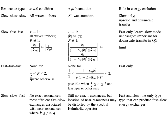
 α≠0
α≠0 k+p=q
k+p=q α
α α=0
α=0 α
α α≠0
α≠0
 α
α Lα=α2/L2
 F=f/N
F=f/N Bu=N2/f2
 Lα
Lα Lα
Lα F
F 2563
2563 10−5
10−5 F
F F
F F
F Lα
Lα y
y Lα
Lα 2563
2563
 Lα
Lα F=f/N
F=f/N F=1/2,1,2
 Lα
Lα Lα
Lα Lα
Lα
 α
α z=0.5
z=0.5 t=0.5
t=0.5 x
x v1
v1 Lα=0
Lα=0 x
x v1
v1 Lα=0.1
 x
x u1
u1 Lα=0.1
 Lα=0.1
 v1
v1 Lα=0
Lα=0 u1
u1 −1
−1
 Lα
Lα F=1
F=1 Bu=1
Bu=1 Lα
Lα Lα
Lα
 F=1
F=1 Bu=1
Bu=1 Lα
Lα
 Lα
Lα F=1/2
F=1/2 Bu=4
Bu=4 Lα
Lα
 F=1/2
F=1/2 Bu=4
Bu=4
 Lα
Lα F=2
F=2 Bu=1/4
 Lα
Lα Lα
Lα 0.025, 0.05, 0.075
 F=2
F=2 Lα
Lα tf=1
tf=1 Lα
Lα
 F=2
F=2 Bu=1/4


 Open access

