





1. Introduction
Steady streaming induced by an oscillating object is a classical phenomenon that has been studied analytically and experimentally (Riley Reference Riley2001). The experimental study of steady streaming around a circular cylinder began with Carrière (Reference Carrière1929) and Andrade (Reference Andrade1931), who examined periodically oscillating air around a cylinder, and reported the now familiar quadrupole-like flow. Schlichting (Reference Schlichting1932) carried out the first asymptotic analysis of steady streaming around a cylinder, and he compared the solution with his experiments on a vibrating cylinder in water. In the small-amplitude limit, he matched the inner boundary layer with the outer potential flow, and his solution became the basis for future analysis. For example, Wang (Reference Wang1968) adapted the layer analysis to include the curvature of the boundary, which is relevant at higher order. Riley (Reference Riley1965) and Stuart (Reference Stuart1966) analysed the problem at high Reynolds number where a second boundary layer exists, and their results agreed well with Schlichting’s experiments. Finally, Holtsmark et al. (Reference Holtsmark, Johnsen, Sikkeland and Skavlem1954) analysed and solved the flow everywhere as a regular perturbation problem.
Though the problem of steady streaming has been studied extensively, past works have primarily focused on single-frequency oscillations, with comparatively less attention to multi-frequency oscillations (Davidson & Riley Reference Davidson and Riley1972; Kotas, Yoda & Rogers Reference Kotas, Yoda and Rogers2008). Davidson & Riley (Reference Davidson and Riley1972) analysed steady streaming of multi-frequency oscillation around a cylinder, and found that the resultant flow is the superposition of steady streaming flows induced by each single-frequency oscillation. Similarly, Kotas et al. (Reference Kotas, Yoda and Rogers2008) experimentally examined the steady flow around a sphere made to oscillate with two frequencies, and they found that the observed flows were the sum of the streaming flows from the respective single-frequency oscillations. The experiments in both of these works were carried out for small-amplitude motion in which the streaming velocity is small, and the asymptotic analysis was only performed up to second order in amplitude. There are reasons to believe that the imposition of multiple oscillatory frequencies might break the spatial symmetry and induce net flow in one direction at higher order in amplitude.
This work is inspired by recent experiments on a different physical system: an object sliding on a surface, undergoing two-frequency lateral oscillation (Hashemi et al. Reference Hashemi, Tahernia, Hui, Ristenpart and Miller2022). Specifically, the surface displacement was $(\ell /2)[\sin (\omega t) + \sin (\alpha \omega t)]$
, where
$(\ell /2)[\sin (\omega t) + \sin (\alpha \omega t)]$
, where $\ell$
is the amplitude,
$\ell$
is the amplitude, $\omega$
is the frequency, and
$\omega$
is the frequency, and $\alpha$
is a ratio of the two frequencies. For particular
$\alpha$
is a ratio of the two frequencies. For particular $\alpha$
values, the object exhibited a net translation. To help to understand the experimental observations, they analysed a model in which the only force considered is the surface contact described by Coulomb’s friction law. Representing the frequency ratio
$\alpha$
values, the object exhibited a net translation. To help to understand the experimental observations, they analysed a model in which the only force considered is the surface contact described by Coulomb’s friction law. Representing the frequency ratio $\alpha$
as
$\alpha$
as $p/q$
, they derived a necessary condition for net motion – one of
$p/q$
, they derived a necessary condition for net motion – one of $p$
or
$p$
or $q$
is odd, and the other is even – and validated this prediction with experiments. For example,
$q$
is odd, and the other is even – and validated this prediction with experiments. For example, $\alpha = 2$
,
$\alpha = 2$
, $3/2$
and
$3/2$
and $1/2$
showed net motion, while
$1/2$
showed net motion, while $\alpha = 1$
,
$\alpha = 1$
, $3$
and
$3$
and $5/3$
did not. We note that the same necessary conditions for directed motion were derived earlier by Reznik & Canny (Reference Reznik and Canny2001) using a simpler friction model (Reznik, Canny & Goldberg Reference Reznik, Canny and Goldberg1997). Additional analysis and experiments for oscillations with different phase and amplitude were carried out in Zhang et al. (Reference Zhang, Hui, Ristenpart and Miller2024a
), and Hui et al. (Reference Hui, Zhang, Adiga, Miller and Ristenpart2024) further corroborated the theory with experiments with granular media.
$5/3$
did not. We note that the same necessary conditions for directed motion were derived earlier by Reznik & Canny (Reference Reznik and Canny2001) using a simpler friction model (Reznik, Canny & Goldberg Reference Reznik, Canny and Goldberg1997). Additional analysis and experiments for oscillations with different phase and amplitude were carried out in Zhang et al. (Reference Zhang, Hui, Ristenpart and Miller2024a
), and Hui et al. (Reference Hui, Zhang, Adiga, Miller and Ristenpart2024) further corroborated the theory with experiments with granular media.
In this work, we use computations and analysis to examine steady streaming around a cylinder, whose oscillation is the sum of two sinusoids of different frequencies. We show that a cylinder vibrating with two-frequency oscillation leads to pumping, i.e. a streaming flow with net directed motion of the surrounding fluid. We apply a small-amplitude analysis to study steady streaming for two-frequency oscillation at low Reynolds numbers. Indeed, at second order in amplitude, steady streaming is a superposition of streaming due to individual frequencies, consistent with prior observations; however, pumping is a higher-order effect and occurs only for certain frequency pairs. Obtaining expressions for higher-order terms is analytically intractable, but the form of the regular perturbation analysis allows us to deduce the structure of the solution and obtain necessary conditions for pumping.
The paper is organised as follows. In § 2, we introduce the motion of the cylinder and the non-dimensionalisation of the fluid equations. In § 3, we present numerical simulations for frequency ratio 2, and compare the flows with those of the single-frequency case. We measure the flux for varying amplitude, and we observe that pumping is a third-order effect. In § 4, we examine the asymptotic analysis of the problem at low amplitude. Even though we cannot solve the equations at third order, we show that a steady solution exists at third order and involves a net force responsible for pumping. Then, in § 5, we expand the analysis to general frequency ratios, and give necessary conditions for pumping, and we predict the order in amplitude at which pumping occurs. Finally, we confirm the theoretical results with computational simulations for select frequency ratios.
2. Problem statement
2.1. Cylinder motion
We use two related formulations of the problem: one in which the cylinder moves, and the other in which the cylinder is stationary and the far-field flow oscillates. For the moving cylinder formulation, a cylinder of radius $R$
and centre
$R$
and centre $(X(t),0)$
moves in a two-dimensional viscous fluid. The horizontal position of the cylinder’s centre is prescribed as
$(X(t),0)$
moves in a two-dimensional viscous fluid. The horizontal position of the cylinder’s centre is prescribed as
 \begin{equation} X(t) = \frac {A}{2}[\sin (\varOmega t) + \sin (\alpha \varOmega t)], \end{equation}
where $A$
is the amplitude of oscillation,
$A$
is the amplitude of oscillation, $\varOmega$
is the angular frequency of the base oscillation, and
$\varOmega$
is the angular frequency of the base oscillation, and $\alpha \geq 1$
, the ratio of the two frequencies. The frequency ratio is assumed rational so that the flow is time-periodic, and if we choose
$\alpha \geq 1$
, the ratio of the two frequencies. The frequency ratio is assumed rational so that the flow is time-periodic, and if we choose $\alpha = 1$
, then we obtain the single-frequency case.
$\alpha = 1$
, then we obtain the single-frequency case.
For analysis, it is convenient to consider the cylinder fixed at the origin, and impose a horizontal flow at infinity of strength
 \begin{equation} U(t) = -\frac {A\varOmega }{2}[\cos (\varOmega t) + \alpha \cos (\alpha \varOmega t)]. \end{equation}
Furthermore, no-slip and no-penetration will be imposed, and the boundary conditions in two-dimensional cylindrical coordinates are
 \begin{equation} u_r(r = R) = 0, \quad u_\theta (r = R) = 0. \end{equation}
The two formulations are related by a change in reference frame. Switching our frame of reference from the inertial frame where the cylinder is oscillating to the non-inertial frame in which the cylinder is fixed results in a fictitious body force (Batchelor Reference Batchelor2000)
 \begin{equation} F = -\rho\, U'(t)\, \boldsymbol{e}_x, \end{equation}
where $\rho$
is the mass density, and
$\rho$
is the mass density, and $\boldsymbol{e}_x$
is the direction vector in the horizontal direction. In the non-inertial frame, we incorporate the fictitious body force (2.4) in the modified pressure defined as
$\boldsymbol{e}_x$
is the direction vector in the horizontal direction. In the non-inertial frame, we incorporate the fictitious body force (2.4) in the modified pressure defined as
 \begin{equation} \tilde {p} = p + \rho x\,U'(t). \end{equation}
For simplicity, we denote the modified pressure as $p$
below.
$p$
below.
2.2. Non-dimensionalisation
The equations are non-dimensionalised using characteristic length scale $R$
, time scale
$R$
, time scale $\varOmega ^{-1}$
, and velocity scale
$\varOmega ^{-1}$
, and velocity scale $R\varOmega$
. The flow around the cylinder is governed by the incompressible Navier Stokes equations:
$R\varOmega$
. The flow around the cylinder is governed by the incompressible Navier Stokes equations:
 \begin{align} {\textit{Re}}\left (\boldsymbol{u_t} + \boldsymbol{u} \boldsymbol{\cdot } \boldsymbol{\nabla }\boldsymbol{u}\right ) &= -\boldsymbol {\nabla }p + \varDelta \boldsymbol{u}, \end{align}
 \begin{align} \boldsymbol {\nabla } \boldsymbol{\cdot }\boldsymbol{u} &= 0, \\[10pt] \nonumber \end{align}
where the Reynolds number is
 \begin{equation} {\textit{Re}} = \frac {R^2\varOmega }{\nu }, \end{equation}
and $\nu$
is the kinematic viscosity. The boundary conditions (2.2) and (2.3) become
$\nu$
is the kinematic viscosity. The boundary conditions (2.2) and (2.3) become
 \begin{equation} u_r(r = 1) = 0, \quad u_\theta (r = 1) = 0, \end{equation}
and the horizontal flow at infinity is
 \begin{equation} U(t) = -\frac {\epsilon }{2}\left [\cos ( t) + \alpha \cos (\alpha t)\right ], \end{equation}
where
 \begin{equation} \epsilon = \frac {A}{R} \end{equation}
is the dimensionless amplitude of oscillation.
The Reynolds number $Re= R^2\varOmega /\nu$
is based on the length scale of the cylinder’s radius, and corresponds to the boundary layer in which viscous forces remain relevant. The streaming Reynolds number
$Re= R^2\varOmega /\nu$
is based on the length scale of the cylinder’s radius, and corresponds to the boundary layer in which viscous forces remain relevant. The streaming Reynolds number ${\textit{Re}}_s$
is based on the length scale of the oscillation amplitude, and it characterises the Reynolds number associated with the streaming flow. The two Reynolds numbers are related by
${\textit{Re}}_s$
is based on the length scale of the oscillation amplitude, and it characterises the Reynolds number associated with the streaming flow. The two Reynolds numbers are related by
 \begin{equation}{\textit{Re}}_s = \frac {A^2\varOmega }{\nu } = \epsilon ^2\, {\textit{Re}}. \end{equation}
The flow structure depends on both ${\textit{Re}}$
and
${\textit{Re}}$
and ${\textit{Re}}_s$
. We refer to figure 1 of Chong et al. (Reference Chong, Kelly, Smith and Eldredge2013) (which is adapted from figure 1 of Wang Reference Wang1968) to illustrate the different flow regimes and associated analyses. Briefly, for high Reynolds numbers, the flow exhibits a boundary layer (Schlichting Reference Schlichting1932; Wang Reference Wang1968), and at high streaming Reynolds numbers, the streaming flow itself develops a second boundary layer (Riley Reference Riley1965; Stuart Reference Stuart1966). At low Reynolds number, the problem can be analysed as a regular perturbation (Holtsmark et al. Reference Holtsmark, Johnsen, Sikkeland and Skavlem1954) – though as noted in Chong et al. (Reference Chong, Kelly, Smith and Eldredge2013), the regular perturbation solution from Holtsmark et al. (Reference Holtsmark, Johnsen, Sikkeland and Skavlem1954) contains the solution from the matched asymptotic analysis of Schlichting (Reference Schlichting1932) and Wang (Reference Wang1968), and is thus appropriate provided that the streaming Reynolds number is small. In this paper, we focus on the low streaming Reynolds number regime
${\textit{Re}}_s$
. We refer to figure 1 of Chong et al. (Reference Chong, Kelly, Smith and Eldredge2013) (which is adapted from figure 1 of Wang Reference Wang1968) to illustrate the different flow regimes and associated analyses. Briefly, for high Reynolds numbers, the flow exhibits a boundary layer (Schlichting Reference Schlichting1932; Wang Reference Wang1968), and at high streaming Reynolds numbers, the streaming flow itself develops a second boundary layer (Riley Reference Riley1965; Stuart Reference Stuart1966). At low Reynolds number, the problem can be analysed as a regular perturbation (Holtsmark et al. Reference Holtsmark, Johnsen, Sikkeland and Skavlem1954) – though as noted in Chong et al. (Reference Chong, Kelly, Smith and Eldredge2013), the regular perturbation solution from Holtsmark et al. (Reference Holtsmark, Johnsen, Sikkeland and Skavlem1954) contains the solution from the matched asymptotic analysis of Schlichting (Reference Schlichting1932) and Wang (Reference Wang1968), and is thus appropriate provided that the streaming Reynolds number is small. In this paper, we focus on the low streaming Reynolds number regime $({\textit{Re}}_s \ll 1)$
so that the problem can be analysed as a regular perturbation, which allows us to compute the structure of solutions beyond second order needed to understand pumping from two-frequency oscillations.
$({\textit{Re}}_s \ll 1)$
so that the problem can be analysed as a regular perturbation, which allows us to compute the structure of solutions beyond second order needed to understand pumping from two-frequency oscillations.
3. Computational studies of frequency ratio 2
We begin by examining the flow patterns of streaming for frequency ratio $\alpha = 2$
using numerical simulations. The numerical methods are described in Appendix C. We consider other frequency ratios in § 5, where we show that
$\alpha = 2$
using numerical simulations. The numerical methods are described in Appendix C. We consider other frequency ratios in § 5, where we show that $\alpha = 2$
yields the strongest pumping, and the difference of the flow pattern from the single-frequency case is subtle for other frequency ratios.
$\alpha = 2$
yields the strongest pumping, and the difference of the flow pattern from the single-frequency case is subtle for other frequency ratios.
3.1. Comparing flow patterns
We place the cylinder in a square $8\times8$
domain with periodic boundary conditions, and solve for the flow at
$8\times8$
domain with periodic boundary conditions, and solve for the flow at $Re= 10$
. We solve for 250 periods, which is sufficiently long to allow the initial transient to decay, and the resulting flows are visualised by the positions of passive marker particles from the previous 10 periods of time. As expected for the single-frequency case in figure 1(a), the flow resembles the classical, four vortices associated with steady streaming. However, for two-frequency motion, shown in figures 1(b,c), the vortices are no longer symmetric and there is a net horizontal flow. The bottom plots show the cylinder’s horizontal position for each case. In figure 1(b), the net flow is left to right – away from the cylinder, the green particles (most current period) are to the right of the blue particles (past period), indicating a net rightward flow. See supplementary movie 1 to compare the flow patterns of single-frequency, two-frequency and reverse two-frequency oscillations. We note that because of the periodic boundary conditions, these simulations correspond to a lattice of oscillating cylinders.
$Re= 10$
. We solve for 250 periods, which is sufficiently long to allow the initial transient to decay, and the resulting flows are visualised by the positions of passive marker particles from the previous 10 periods of time. As expected for the single-frequency case in figure 1(a), the flow resembles the classical, four vortices associated with steady streaming. However, for two-frequency motion, shown in figures 1(b,c), the vortices are no longer symmetric and there is a net horizontal flow. The bottom plots show the cylinder’s horizontal position for each case. In figure 1(b), the net flow is left to right – away from the cylinder, the green particles (most current period) are to the right of the blue particles (past period), indicating a net rightward flow. See supplementary movie 1 to compare the flow patterns of single-frequency, two-frequency and reverse two-frequency oscillations. We note that because of the periodic boundary conditions, these simulations correspond to a lattice of oscillating cylinders.
Streaming flows at time $T = 250$
for amplitude
$T = 250$
for amplitude $0.5$
and Reynolds number
$0.5$
and Reynolds number $10$
for (a) single-frequency motion, (b) two-frequency motion, and (c) two-frequency motion with time reversal. Shown are the positions of passive tracer particles over
$10$
for (a) single-frequency motion, (b) two-frequency motion, and (c) two-frequency motion with time reversal. Shown are the positions of passive tracer particles over $10$
periods, where the current location is coloured green, and the location
$10$
periods, where the current location is coloured green, and the location $10$
periods prior is coloured blue. The domain is
$10$
periods prior is coloured blue. The domain is $8\times8$
with periodic boundary conditions. The bottom plots show the horizontal position of the cylinder’s centre over one period.
$8\times8$
with periodic boundary conditions. The bottom plots show the horizontal position of the cylinder’s centre over one period.

Figure 1(c) shows the flow resulting from the time-reversed, two-frequency motion of the cylinder. In this case, the flow is moving right to left, and the flow pattern appears to be the reflection about the vertical axis of the flow pattern from figure 1(b). The waveforms of the cylinders’ positions for all three cases are depicted in the bottom row of figure 1. Note that the time-reversed waveform of the two-frequency oscillation is not a phase shift of the original, as in the single-frequency case. For the time-reversed oscillation, the flow is moving right to left, and the flow pattern appears to be the reflection about the vertical axis of the flow pattern from figure 1(b). This result demonstrates that the direction of the net flow is determined by the time asymmetry of the cylinder’s motion. In the discussion, we elaborate on how the time symmetry of the cylinder motion for different frequency ratios is related to pumping. We note that a similar result was observed in the experiments of Hashemi et al. (Reference Hashemi, Tahernia, Hui, Ristenpart and Miller2022) and Hui et al. (Reference Hui, Zhang, Adiga, Miller and Ristenpart2024). When they reversed the polarity of the motion, the object translated in the opposite direction.
3.2. Pumping in a channel
The results in figure 1(b) suggest that cylinders oscillating with two frequencies can be used to pump fluids. To test that idea more directly, we repeated the computational experiments in a channel of height 8 and length 32, with no-slip boundary conditions on the top and bottom, and periodic conditions in the horizontal direction. Figure 2 is a picture of supplementary movie 2 at time $T = 250$
, showing the contrast of single- and two-frequency motions inside a channel. Again, for the single-frequency case, the four vortices align symmetrically around the cylinder, and particles away from the cylinder remain stationary. However, when the cylinder oscillates with two frequencies, the vortices lose their symmetry, and fluid is pumped to the right. Applying the negative waveform again reversed the direction of motion (results not shown).
$T = 250$
, showing the contrast of single- and two-frequency motions inside a channel. Again, for the single-frequency case, the four vortices align symmetrically around the cylinder, and particles away from the cylinder remain stationary. However, when the cylinder oscillates with two frequencies, the vortices lose their symmetry, and fluid is pumped to the right. Applying the negative waveform again reversed the direction of motion (results not shown).
Streaming flows in a $32\times8$
channel for (a) single-frequency (
$32\times8$
channel for (a) single-frequency ( $\alpha = 1$
) and (b) two-frequency (
$\alpha = 1$
) and (b) two-frequency ( $\alpha = 2$
) oscillations at time
$\alpha = 2$
) oscillations at time $T = 250$
visualised with amplitude
$T = 250$
visualised with amplitude $\epsilon = 0.7$
and Reynolds number
$\epsilon = 0.7$
and Reynolds number $10$
. Passive tracer particles highlight the positions of the flow from the last
$10$
. Passive tracer particles highlight the positions of the flow from the last $10$
periods. Shown are the positions of passive tracer particles over
$10$
periods. Shown are the positions of passive tracer particles over $10$
periods, where the current location is coloured green, and the location
$10$
periods, where the current location is coloured green, and the location $10$
periods prior is coloured blue.
$10$
periods prior is coloured blue.

Figure 3(a) shows the flux through a channel of height $H$
,
$H$
,
 \begin{equation} Q(t) = \int _{0}^{H} u(x, y, t)\,{\rm d}y, \end{equation}
over $5$
periods for both the single- and two-frequency cases for amplitude
$5$
periods for both the single- and two-frequency cases for amplitude $\epsilon =0.9$
. The flux for the two-frequency case shows a non-zero average flux on the scale of approximately 10 % of the amplitude of the oscillation. We quantify pumping by the time average of the flux over the period
$\epsilon =0.9$
. The flux for the two-frequency case shows a non-zero average flux on the scale of approximately 10 % of the amplitude of the oscillation. We quantify pumping by the time average of the flux over the period $T$
:
$T$
:
 \begin{equation} \langle Q(t)\rangle \;= \frac {1}{T}\int _{t - T}^{t} Q(\tau )\, {\rm d}\tau . \end{equation}
Figure 3(b) shows the period-averaged flux as a function of time for different amplitudes. For each amplitude, the period-averaged flux approaches a steady value that depends on the amplitude. The time-reversed oscillation results in the negative of the flux for the non-reversed oscillation of the same amplitude.
(a) Flux versus time is presented for both the single- and two-frequency cases for amplitude 0.9 and Reynolds number 10. (b) Time-averaged fluxes are shown for varying amplitudes $\epsilon$
. (c) The steady time-averaged flux is third order in amplitude for two-frequency oscillations. (d) The size of the oscillatory component,
$\epsilon$
. (c) The steady time-averaged flux is third order in amplitude for two-frequency oscillations. (d) The size of the oscillatory component, $\langle \|u\|_2\rangle$
, is first order in amplitude, and the size of the steady streaming flow,
$\langle \|u\|_2\rangle$
, is first order in amplitude, and the size of the steady streaming flow, $\|\langle u\rangle \|_2$
, is second order in amplitude for the two-frequency oscillation.
$\|\langle u\rangle \|_2$
, is second order in amplitude for the two-frequency oscillation.

Figure 3(c) shows that the steady flux grows like amplitude cubed. For single-frequency oscillations, the magnitude of the steady flow is second order in amplitude, and the oscillatory component is first order (Holtsmark et al. Reference Holtsmark, Johnsen, Sikkeland and Skavlem1954; Wang Reference Wang1968; Chong et al. Reference Chong, Kelly, Smith and Eldredge2013). In figure 3(d), we show that for the two-frequency case, these same scalings for the sizes of the steady and oscillatory flows result as measured by the $2$
-norm of the period-averaged flow and the time average of the
$2$
-norm of the period-averaged flow and the time average of the $2$
-norm of the velocity, respectively. Previously, analysis on steady streaming has only been carried out to second order in amplitude, so to derive the terms responsible for pumping, we need to extend the analysis to third order.
$2$
-norm of the velocity, respectively. Previously, analysis on steady streaming has only been carried out to second order in amplitude, so to derive the terms responsible for pumping, we need to extend the analysis to third order.
3.3. Effect of Reynolds number on pumping
We repeat the computational studies from the previous section at amplitude $\epsilon = 0.5$
and time
$\epsilon = 0.5$
and time ${T} = 300$
to examine how the flux and flow structure change with Reynolds number. We note that at
${T} = 300$
to examine how the flux and flow structure change with Reynolds number. We note that at ${\textit{Re}} = 0$
, the time-averaged flow is zero because of the dynamic reversibility of Stokes flow, and thus, there is no pumping at zero Reynolds number. Figure 4 shows the time-averaged flux for
${\textit{Re}} = 0$
, the time-averaged flow is zero because of the dynamic reversibility of Stokes flow, and thus, there is no pumping at zero Reynolds number. Figure 4 shows the time-averaged flux for $10\leq {\textit{Re}}\leq 100$
at amplitude
$10\leq {\textit{Re}}\leq 100$
at amplitude $\epsilon = 0.5$
, frequency ratio
$\epsilon = 0.5$
, frequency ratio $\alpha = 2$
, and time
$\alpha = 2$
, and time ${T} = 300$
. The flux grows with Reynolds number at a rate slightly larger than
${T} = 300$
. The flux grows with Reynolds number at a rate slightly larger than $\sqrt {{\textit{Re}}}$
.
$\sqrt {{\textit{Re}}}$
.
At amplitude $\epsilon = 0.5$
, frequency ratio
$\epsilon = 0.5$
, frequency ratio $\alpha = 2$
, and time
$\alpha = 2$
, and time ${T} = 300$
, the time-averaged fluxes for a
${T} = 300$
, the time-averaged fluxes for a $32\times8$
channel are measured for various Reynolds numbers. In general, the time-averaged fluxes appear to scale at a rate slightly larger than
$32\times8$
channel are measured for various Reynolds numbers. In general, the time-averaged fluxes appear to scale at a rate slightly larger than $\sqrt {{\textit{Re}}}$
.
$\sqrt {{\textit{Re}}}$
.

In figure 5, we show the streamlines and normalised velocity vectors of the time-averaged flow for both single- and two-frequency cases at $\textit{Re}=10$
and
$\textit{Re}=10$
and $\textit{Re}=50$
, which are above and below the critical Reynolds number (Chong et al. Reference Chong, Kelly, Smith and Eldredge2013) at which a boundary layer forms. At
$\textit{Re}=50$
, which are above and below the critical Reynolds number (Chong et al. Reference Chong, Kelly, Smith and Eldredge2013) at which a boundary layer forms. At $\textit{Re}=10$
for the single-frequency case, we see the classical quadrupole-like structure, where the red streamlines indicate anticlockwise flow, and the blue streamlines indicate clockwise flow (figure 5
a). For frequency ratio
$\textit{Re}=10$
for the single-frequency case, we see the classical quadrupole-like structure, where the red streamlines indicate anticlockwise flow, and the blue streamlines indicate clockwise flow (figure 5
a). For frequency ratio $\alpha = 2$
, there is a clear flow to the right, and vortices are no longer left–right symmetric. At
$\alpha = 2$
, there is a clear flow to the right, and vortices are no longer left–right symmetric. At $\textit{Re}=50$
, for both the single- and two-frequency cases, there is a region near the cylinder consisting of four rotating vortices with counter-rotating vortices outside this area (figures 5
c,d). For two-frequency oscillations, the net flow passes between the inner and outer vortices downstream from the cylinder. It should be noted that the near-cylinder region containing the inner vortices in figures 5(b,d) is sometimes referred to as the DC boundary layer to distinguish it from the thinner boundary layer associated with the oscillatory flow (Raney, Corelli & Westervelt Reference Raney, Corelli and Westervelt1954; Bertelsen, Svardal & Tjøtta Reference Bertelsen, Svardal and Tjøtta1973; Lutz, Chen & Schwartz Reference Lutz, Chen and Schwartz2005; Chong et al. Reference Chong, Kelly, Smith and Eldredge2013).
$\textit{Re}=50$
, for both the single- and two-frequency cases, there is a region near the cylinder consisting of four rotating vortices with counter-rotating vortices outside this area (figures 5
c,d). For two-frequency oscillations, the net flow passes between the inner and outer vortices downstream from the cylinder. It should be noted that the near-cylinder region containing the inner vortices in figures 5(b,d) is sometimes referred to as the DC boundary layer to distinguish it from the thinner boundary layer associated with the oscillatory flow (Raney, Corelli & Westervelt Reference Raney, Corelli and Westervelt1954; Bertelsen, Svardal & Tjøtta Reference Bertelsen, Svardal and Tjøtta1973; Lutz, Chen & Schwartz Reference Lutz, Chen and Schwartz2005; Chong et al. Reference Chong, Kelly, Smith and Eldredge2013).
For a $32\times8$
channel at amplitude
$32\times8$
channel at amplitude $\epsilon = 0.5$
and time
$\epsilon = 0.5$
and time ${T} = 300$
, the streamlines and the flow directions (normalised velocity field) of the time-averaged flow are shown at frequency ratios (a,c)
${T} = 300$
, the streamlines and the flow directions (normalised velocity field) of the time-averaged flow are shown at frequency ratios (a,c) $\alpha = 1$
and (b,d)
$\alpha = 1$
and (b,d) $\alpha = 2$
, for (a,b)
$\alpha = 2$
, for (a,b) ${\textit{Re}} = 10$
and (c,d)
${\textit{Re}} = 10$
and (c,d) ${\textit{Re}} = 50$
.
${\textit{Re}} = 50$
.

4. Low-amplitude analysis
We now analyse the problem in the limit of small amplitude $(\epsilon \ll 1)$
, and we restrict our analysis to small streaming Reynolds numbers
$(\epsilon \ll 1)$
, and we restrict our analysis to small streaming Reynolds numbers $({\textit{Re}}_s \ll 1)$
to apply a regular perturbation. The single-frequency solution has been previously computed through second order in amplitude (Holtsmark et al. Reference Holtsmark, Johnsen, Sikkeland and Skavlem1954; Chong et al. Reference Chong, Kelly, Smith and Eldredge2013), but extending the analysis to third order is not analytically tractable. However, we derive the structure of the higher-order solutions, and from the structure alone, we can understand why pumping is a third-order effect for the two-frequency case.
$({\textit{Re}}_s \ll 1)$
to apply a regular perturbation. The single-frequency solution has been previously computed through second order in amplitude (Holtsmark et al. Reference Holtsmark, Johnsen, Sikkeland and Skavlem1954; Chong et al. Reference Chong, Kelly, Smith and Eldredge2013), but extending the analysis to third order is not analytically tractable. However, we derive the structure of the higher-order solutions, and from the structure alone, we can understand why pumping is a third-order effect for the two-frequency case.
4.1. Governing equations
We analyse the problem in terms of the stream function $\psi$
, which is related to the velocity by
$\psi$
, which is related to the velocity by
 \begin{equation} u_r = \frac {1}{r}\frac {\partial \psi }{\partial \theta }, \quad u_\theta = -\frac {\partial \psi }{\partial r}, \end{equation}
and
 \begin{equation} \boldsymbol{\nabla }\times \boldsymbol{u} = -\varDelta \psi . \end{equation}
We take the curl of the momentum (2.6) to obtain
 \begin{equation} \left (\varDelta - {\textit{Re}}\frac {\partial }{\partial t}\right )\varDelta \psi = {\textit{Re}}\,\boldsymbol{u} \boldsymbol{\cdot } \boldsymbol{\nabla }\left (\varDelta \psi \right )\!. \end{equation}
We solve the problem in the reference frame in which the cylinder is stationary with an oscillatory flow at infinity. The boundary conditions in terms of the stream function are
 \begin{align}&\qquad\,\, \psi (r = 1) = 0, \quad \frac {\partial \psi }{\partial r}(r = 1) = 0, \end{align}
 \begin{align}& \psi \sim -\frac {\epsilon r}{2}\left (\cos (t) + 2\cos (2t)\right )\sin (\theta ), \quad r \rightarrow \infty . \end{align}
We consider the low-amplitude limit, and expand the solution in terms of $\epsilon = A/R$
:
$\epsilon = A/R$
:
 \begin{align} \psi = \epsilon \psi _1 + \epsilon ^2\psi _2 + \epsilon ^3\psi _3 + O\big (\epsilon ^4\big ). \end{align}
Substituting the expansion into (4.3), (4.4) and (4.5), we obtain the successive equations at each order:
 \begin{align}&\quad\qquad\qquad\qquad\qquad\textbf{First Order}\nonumber\\[-3pt] &\qquad\qquad\qquad \left (\varDelta - {\textit{Re}}\frac {\partial }{\partial t}\right )\varDelta \psi _1 = 0, \end{align}
 \begin{align}&\qquad\qquad \psi _1(r = 1) = 0, \quad \frac {\partial \psi _1}{\partial r}(r = 1) = 0, \end{align}
 \begin{align}&\qquad \psi _1 \sim -\frac {r}{2}\left (\cos (t) + 2\cos (2t)\right )\sin (\theta ), \quad r \rightarrow \infty. \end{align}
 \begin{align}&\quad\qquad\qquad\qquad\qquad\textbf{Second Order}\nonumber\\[0pt] &\quad\qquad\quad \left (\varDelta - {\textit{Re}}\frac {\partial }{\partial t}\right )\varDelta \psi _2 = {\textit{Re}}\, \boldsymbol{u_1}\boldsymbol{\cdot }\boldsymbol{\nabla }\left (\varDelta \psi _1\right )\!, \end{align}
 \begin{align}&\qquad\qquad\quad \psi _2(r = 1) = 0, \quad \frac {\partial \psi _2}{\partial r}(r = 1) = 0, \end{align}
 \begin{align}&\qquad\qquad\qquad\qquad\,\, \psi _2 \sim 0, \quad r \rightarrow \infty. \end{align}
 \begin{align}&\nonumber\\[-9pt]&\quad\qquad\qquad\qquad\qquad\textbf{Third Order}\nonumber\\[0pt]& \left (\varDelta - {\textit{Re}}\frac {\partial }{\partial t}\right )\varDelta \psi _3 = {\textit{Re}}\, \boldsymbol{u_1} \boldsymbol{\cdot }\boldsymbol {\nabla }\left (\varDelta \psi _2\right ) + {\textit{Re}}\, \boldsymbol{u_2} \boldsymbol{\cdot } \boldsymbol{\nabla }\left (\varDelta \psi _1\right )\!, \end{align}
 \begin{align}&\qquad\qquad\qquad \psi _3(r = 1) = 0, \quad \frac {\partial \psi _3}{\partial r}(r = 1) = 0, \end{align}
 \begin{align}&\qquad\qquad\qquad\qquad\quad \psi _3 \sim 0, \quad r \rightarrow \infty . \end{align}
4.2. Solution structure
4.2.1. Single-frequency oscillation
Before we consider the two-frequency case, we first examine the solution structure for single-frequency oscillation. The only difference in the equations for the single-frequency and two-frequency cases is the boundary condition at infinity at first order. For the single-frequency case, (4.9) is replaced by
 \begin{equation} \psi _1 \sim -r\cos (t)\sin (\theta ). \end{equation}
This boundary condition determines the form of the solution at first order as
 \begin{equation} \psi _1 = \textrm{Re} \big (a_1(r)\,\textrm{e}^{-\textrm{i}\textit{t}}\big )\sin (\theta ), \end{equation}
where $\textrm{Re} (z )$
denotes the real part of
$\textrm{Re} (z )$
denotes the real part of $z$
. Analytically,
$z$
. Analytically, $a_1(r)$
is a solution composed of Hankel functions (Watson Reference Watson1922). We substitute (4.17) into the quadratic nonlinearity on the right-hand side of (4.10) to determine the form of the solution at second order. This computation involves all products of
$a_1(r)$
is a solution composed of Hankel functions (Watson Reference Watson1922). We substitute (4.17) into the quadratic nonlinearity on the right-hand side of (4.10) to determine the form of the solution at second order. This computation involves all products of $\textrm{e}^{-\textrm{i}\textit{t}}$
and
$\textrm{e}^{-\textrm{i}\textit{t}}$
and $\textrm{e}^{\textrm{i}\textit{t}}$
, which results in a steady term and terms proportional to
$\textrm{e}^{\textrm{i}\textit{t}}$
, which results in a steady term and terms proportional to $\textrm{e}^{\pm \textrm{i}2t}$
. Therefore, at second order, we obtain
$\textrm{e}^{\pm \textrm{i}2t}$
. Therefore, at second order, we obtain
 \begin{equation} \psi _2 = \textrm{Re} \big (b_2(r)\,\textrm{e}^{-2\textrm{i}t}\big )\sin (2\theta ) + b_0(r)\sin (2\theta ). \end{equation}
Equation (4.13) at third order involves products of (4.17) and (4.18) on its right-hand side. This computation involves products of $\textrm{e}^{\pm \textrm{i}t}$
with 1 and with
$\textrm{e}^{\pm \textrm{i}t}$
with 1 and with $\textrm{e}^{\pm 2\textrm{i}t}$
, which results in terms proportional to
$\textrm{e}^{\pm 2\textrm{i}t}$
, which results in terms proportional to $\textrm{e}^{\pm \textrm{i}3t}$
and
$\textrm{e}^{\pm \textrm{i}3t}$
and $\textrm{e}^{\pm \textrm{i}t}$
. The third-order solution is of the form
$\textrm{e}^{\pm \textrm{i}t}$
. The third-order solution is of the form
 \begin{equation} \psi _3 = \textrm{Re} \big (c_3(r)\,\textrm{e}^{-\textrm{i}3t} + c_1(r)\,\textrm{e}^{-\textit{\textrm{i}t}}\big )\sin (3\theta ) + \textrm{Re} \big (d_3(r)\,\textrm{e}^{-\textrm{i}3t} + d_1(r)\,\textrm{e}^{-\textrm{i}\textit{t}}\big )\sin (\theta ). \end{equation}
Therefore, for the single-frequency case, there is no steady term at third order.
4.2.2. Two-frequency oscillation
For the two-frequency case, we obtain
 \begin{equation} \psi _1 = \textrm{Re} \big (a_1(r)\,\textrm{e}^{-\textrm{i}\textit{t}} + a_2(r)\,\textrm{e}^{-2\textrm{i}t}\big )\sin (\theta ) \end{equation}
as the solution to (4.7)–(4.9). As before, we substitute the solution at first order into the right-hand side of (4.10) to deduce the structure of the second-order solution as
 \begin{eqnarray} \psi _2 & = & \textrm{Re} \left (\sum _{k=1}^{4}b_k(r)\,\textrm{e}^{-\textrm{i}kt}\right )\sin (2\theta ) + b_0^{(1)}(r)\sin (2\theta ) + b_0^{(2)}(r)\sin (2\theta ) \nonumber \\&=& \textrm{Re} \big (\big (b_{2}(r)\,\textrm{e}^{-2\textrm{i}t}+ b_0^{(1)}(r)\big ) + \big (b_{4}(r)\,\textrm{e}^{-4\textrm{i}t}+ b_0^{(2)}(r)\big ) \nonumber \\&& \mbox{} + \big (b_{1}(r)\,\textrm{e}^{-\textrm{i}\textit{t}}+ b_{3}(r)\,\textrm{e}^{-3\textrm{i}t}\big )\big )\sin (2\theta ). \end{eqnarray}
We express the solution in this second form with three pairs of terms grouped together to highlight the origins of the different terms in the sum. The first two pairs involving a steady term and unsteady term correspond to the single-frequency solutions from each of the two driving frequencies, and the last pair of unsteady terms arises from the interaction between the driving frequencies. Thus as has been reported previously, the steady flow at second order is the superposition of two streaming fields caused by the individual, single-frequency oscillations (Davidson & Riley Reference Davidson and Riley1972; Kotas et al. Reference Kotas, Yoda and Rogers2008).
The nonlinear interaction between the two frequencies only affects the unsteady terms at second order, but these interactions produce a steady flow at third order. The solution at third order has the form
 \begin{eqnarray} \psi _3 & = & \textrm{Re} \left (\sum _{k=1}^6 c_k(r)\,\textrm{e}^{-\textrm{i}kt}\right )\sin (3\theta ) + c_0(r)\sin (3\theta ) \nonumber \\ && \mbox{} + \textrm{Re} \left (\sum _{k=1}^6 d_k(r)\,\textrm{e}^{-\textrm{i}kt}\right )\sin (\theta ) + d_0(r)\sin (\theta ). \end{eqnarray}
Unlike the single-frequency solution (4.19), there are steady terms at third order in amplitude. In the following subsections, we explain how the third-order, steady terms produce the observed left–right asymmetry and are responsible for producing a net force that pumps the fluid.
4.3. Symmetry of steady flow
To illustrate how the steady flows at third order create asymmetry, consider the steady solution
 \begin{equation} \psi ^s = \epsilon ^2\, b(r)\sin (2\theta ) + \epsilon ^3\, c(r)\sin (3\theta ) + \epsilon ^3\, d(r)\sin (\theta ) + O\big (\epsilon ^4\big ). \end{equation}
We show that the familiar second-order flow has a spatial symmetry different from that of the third-order flow that arises from the interactions of the flows generated by the two different driving frequencies. Specifically, the spatial symmetry arises from the $\theta$
-dependence of the stream functions. To illustrate these symmetries, we examine the streamlines of the three stream functions
$\theta$
-dependence of the stream functions. To illustrate these symmetries, we examine the streamlines of the three stream functions
 \begin{equation} \psi _2 = f(r)\sin (2\theta ),\quad \psi _3^{(1)} = f(r)\sin (\theta ),\quad \psi _3^{(3)} = f(r)\sin (3\theta ), \end{equation}
where
 \begin{equation} f(r) = \frac {(r-1)^2}{1 + r^4}. \end{equation}
This choice of $f(r)$
satisfies the boundary conditions on the cylinder and decays to zero at infinity, but it is not related to the solution of the equations.
$f(r)$
satisfies the boundary conditions on the cylinder and decays to zero at infinity, but it is not related to the solution of the equations.
The streamlines of $\psi _2, \psi _3^{(1)}, \psi _3^{(3)}$
are shown in figures 6(a–c), while the streamlines of the weighted sum are presented in figure 6(d). All the terms share a common up–down symmetry where the values at the points reflected across the horizontal axis are opposite in sign. Specifically, the stream functions are odd in
$\psi _2, \psi _3^{(1)}, \psi _3^{(3)}$
are shown in figures 6(a–c), while the streamlines of the weighted sum are presented in figure 6(d). All the terms share a common up–down symmetry where the values at the points reflected across the horizontal axis are opposite in sign. Specifically, the stream functions are odd in $y$
, i.e.
$y$
, i.e.
 \begin{equation} \psi _2(x, -y) =-\psi _2(x,y), \quad \psi _3^{(1)}(x, -y) = -\psi _3^{(1)}(x, y), \quad \psi _3^{(3)}(x, -y) = -\psi _3^{(3)}(x, y), \end{equation}
and the sum of the stream functions maintains this up–down symmetry. However, $\psi _2$
has a different left–right symmetry from the symmetry shared by the
$\psi _2$
has a different left–right symmetry from the symmetry shared by the $\psi _3$
terms. Specifically,
$\psi _3$
terms. Specifically, $\psi _2$
is odd in
$\psi _2$
is odd in $x$
, while the
$x$
, while the $\psi _3$
terms are even in
$\psi _3$
terms are even in $x$
:
$x$
:
 \begin{equation} \psi _2(-x, y) =-\psi _2(x,y), \quad \psi _3^{(1)}(-x, y) = \psi _3^{(1)}(x, y), \quad \psi _3^{(3)}(-x, y) = \psi _3^{(3)}(x, y). \end{equation}
Therefore, the sum of the stream functions, illustrated in figure 6(d), retains the up–down symmetry, but lacks the left–right symmetry.
The contours of the stream functions are shown for (a) $\psi _2 = f(r)\sin (2\theta )$
, (b)
$\psi _2 = f(r)\sin (2\theta )$
, (b) $\psi _3^{(1)} = f(r)\sin (\theta )$
, and (c)
$\psi _3^{(1)} = f(r)\sin (\theta )$
, and (c) $\psi _3^{(3)} = f(r)\sin (3\theta )$
, where
$\psi _3^{(3)} = f(r)\sin (3\theta )$
, where $f(r)$
is defined by (4.25). (d) Streamlines of the sum
$f(r)$
is defined by (4.25). (d) Streamlines of the sum $\psi = \epsilon ^2 f(r)\sin (2\theta ) + \epsilon ^3 f(r)\sin (3\theta ) + \epsilon ^3 f(r)\sin (\theta )$
for
$\psi = \epsilon ^2 f(r)\sin (2\theta ) + \epsilon ^3 f(r)\sin (3\theta ) + \epsilon ^3 f(r)\sin (\theta )$
for $\epsilon = 0.45$
exhibit a left–right asymmetry.
$\epsilon = 0.45$
exhibit a left–right asymmetry.

4.4. Net force
We compute the net force on the cylinder, and show that the steady term proportional to $\sin (\theta )$
that appears at third order for two-frequency oscillations indicates that there is a net force on the cylinder. Assume a steady solution of the form
$\sin (\theta )$
that appears at third order for two-frequency oscillations indicates that there is a net force on the cylinder. Assume a steady solution of the form
 \begin{equation} \psi ^s = \sum _{k = 1}^\infty f_k(r)\sin (k\theta ). \end{equation}
The pressure can be computed using the momentum (2.6) to obtain
 \begin{equation} p^s = p_\infty + \sum _{k=1}^\infty g_k(r)\cos (k\theta ). \end{equation}
The traction force in the horizontal direction is
 \begin{equation} \left (\sigma \boldsymbol{\cdot }\hat {e}_r\right )\boldsymbol{\cdot }\hat {e}_x = \sigma _{rr}\cos (\theta ) - \sigma _{r\theta }\sin (\theta ), \end{equation}
where $\hat {e}_{r}$
and
$\hat {e}_{r}$
and $\hat {e}_x$
are the direction vectors for the
$\hat {e}_x$
are the direction vectors for the $r$
- and
$r$
- and $x$
-directions, respectively, and
$x$
-directions, respectively, and $\sigma$
is the stress tensor. Using the boundary conditions on the cylinder from (2.9), the components of the stress on the cylinder are
$\sigma$
is the stress tensor. Using the boundary conditions on the cylinder from (2.9), the components of the stress on the cylinder are
 \begin{equation} \sigma _{rr} = -p_{\infty } - \sum _{k=1}^{\infty }g_k(1)\cos (k\theta ), \quad \sigma _{r\theta } = -\sum _{k=1}^{\infty }f_k^{\prime\prime}(1)\sin (k\theta ). \end{equation}
Integrating the surface stress (4.30) over the cylinder, all the terms corresponding to $k \geq 2$
vanish due to symmetry, and the net horizontal force is
$k \geq 2$
vanish due to symmetry, and the net horizontal force is
 \begin{equation} \text{net force} = \int _0^{2\pi } \bigl(\sigma _{rr}\cos (\theta ) - \sigma _{r\theta }\sin (\theta )\bigr)\,{\rm d}\theta = \pi \left (-g_1(1) + f_1^{\prime\prime}(1)\right )\!. \end{equation}
Therefore the term proportional to $\sin (\theta )$
that appears at third order in (4.23) contributes a net force that is responsible for the observed pumping.
$\sin (\theta )$
that appears at third order in (4.23) contributes a net force that is responsible for the observed pumping.
This force calculation gives insight as to why pumping does not occur for the single-frequency case. From § 4.2.1, the only steady term through third order in amplitude is proportional to $\sin (2\theta )$
, and the only non-zero term in the pressure expansion, (4.29), is proportional to
$\sin (2\theta )$
, and the only non-zero term in the pressure expansion, (4.29), is proportional to $\cos (2\theta )$
. Therefore there is no net force for single-frequency oscillations through third order in amplitude, though we have not yet considered the possibility of a net force resulting at higher order for the single-frequency case. In the next section, we analyse the form of the solution at higher orders, and we extend the analysis to general frequency ratio to derive necessary conditions on the frequency ratio for pumping.
$\cos (2\theta )$
. Therefore there is no net force for single-frequency oscillations through third order in amplitude, though we have not yet considered the possibility of a net force resulting at higher order for the single-frequency case. In the next section, we analyse the form of the solution at higher orders, and we extend the analysis to general frequency ratio to derive necessary conditions on the frequency ratio for pumping.
5. Analysis of general frequency ratios
In the previous section, we showed that the steady stream function for frequency ratio $\alpha =2$
contained a term at third order proportional to
$\alpha =2$
contained a term at third order proportional to $\sin (\theta )$
. In this section, we examine the solution structure of
$\sin (\theta )$
. In this section, we examine the solution structure of $\psi _n$
, the solution to the
$\psi _n$
, the solution to the $n$
th-order perturbative equation (5.6), to determine whether there is potentially a net force on the fluid due to the presence of a
$n$
th-order perturbative equation (5.6), to determine whether there is potentially a net force on the fluid due to the presence of a $\sin (\theta )$
term in the expansion, and if so, what order.
$\sin (\theta )$
term in the expansion, and if so, what order.
For this analysis, it is convenient to express the motion of the cylinder as
 \begin{equation} X(t) = \frac {\epsilon }{2}\left (\sin (a t) + \sin (b t)\right )\!, \end{equation}
where $\text{gcd}(a, b) = 1$
. This expression is a slight modification from (2.1), and it amounts to a different definition of the Reynolds number from the one used in the previous sections. We again change reference frames by fixing the cylinder, and the governing equations have the form
$\text{gcd}(a, b) = 1$
. This expression is a slight modification from (2.1), and it amounts to a different definition of the Reynolds number from the one used in the previous sections. We again change reference frames by fixing the cylinder, and the governing equations have the form
 \begin{align}&\qquad\,\, \left (\varDelta - {\textit{Re}}\frac {\partial }{\partial t}\right )\varDelta \psi = {\textit{Re}}\,\boldsymbol{u}\boldsymbol {\cdot } \boldsymbol{\nabla }\left (\varDelta \psi \right )\!, \end{align}
 \begin{align}&\qquad\quad\,\, \psi (r = 1) = 0, \quad \frac {\partial \psi }{\partial r}(r = 1) = 0, \end{align}
 \begin{align}& \psi \sim -\frac {\epsilon r }{2} \left (a\cos (a t) + b\cos (bt)\right )\sin (\theta ), \quad r \rightarrow \infty . \end{align}
Expanding
 \begin{equation} \psi = \epsilon \psi _1 + \epsilon ^2\psi _2 + \epsilon ^3\psi _3 + O\big (\epsilon ^4\big ) \end{equation}
in the low-amplitude limit, and substituting this expansion into (5.2), we obtain successive equations of the form
 \begin{equation} \varDelta \left (\varDelta - {\textit{Re}}\;\frac {\partial }{\partial t}\right ) \psi _n = \sum _{i+j = n} {\textit{Re}}\,\boldsymbol{u}_i \boldsymbol {\cdot } \boldsymbol{\nabla }(\varDelta \psi _j). \end{equation}
The boundary conditions on the cylinder at each order are
 \begin{equation} \psi _n(r = 1) = 0, \quad \frac {\partial \psi _n}{\partial r}(r = 1) = 0, \end{equation}
and the asymptotic condition at $r=\infty$
is
$r=\infty$
is
 \begin{equation} \psi _n \sim \begin{cases} \dfrac {-r}{2}\left (a\cos (at) + b\cos (bt)\right )\sin (\theta ), & n = 1, \ r\rightarrow \infty, \\[5pt] 0, & n \gt 1, \ r\rightarrow \infty . \end{cases} \end{equation}
The solution to (5.6)–(5.8) is of the form
 \begin{equation} \psi _{n} = \sum _{m=1}^{\infty }\sum _{k,m=-\infty }^{\infty } f^{n}_{k,m}(r)\sin \left (m\theta \right )\textrm{e}^{\textrm{i}\textit{kt}}, \end{equation}
but the number of non-zero terms is finite at each order. The boundary condition determines the non-zero terms at leading order, and at higher orders, the structure of the solution depends on the products of the lower-order terms. In the following subsections, we first determine which terms proportional to $\sin (m\theta )$
are non-zero at each order, then derive conditions for the presence of a steady term (
$\sin (m\theta )$
are non-zero at each order, then derive conditions for the presence of a steady term ( $k=0$
).
$k=0$
).
5.1. The $\theta$
-dependent terms
$\theta$
-dependent terms

From the form of the far-field boundary condition (5.8), the leading-order solution is of the form
 \begin{equation} \psi _1 = \textrm{Re} \left (a_2(r)\,\textrm{e}^{-\textrm{i}bt} + a_1(r)\,\textrm{e}^{-\textrm{i}\textit{at}}\right )\sin (\theta ) = C_1(r,t)\sin (\theta ). \end{equation}
The form of the right-hand side of (5.6) dictates the solution structure at higher orders. Substituting $\psi _1$
into the quadratic nonlinearity, the right-hand side of (5.6) is proportional to
$\psi _1$
into the quadratic nonlinearity, the right-hand side of (5.6) is proportional to $\sin (\theta )\cos (\theta )$
, thus the solution is proportional to
$\sin (\theta )\cos (\theta )$
, thus the solution is proportional to $\sin (2\theta )$
. Therefore,
$\sin (2\theta )$
. Therefore, $\psi _2$
is of the form
$\psi _2$
is of the form
 \begin{align} \psi _2 &= \displaystyle \textrm{Re} \left (b_4(r)\,\textrm{e}^{-\textrm{i}2bt} + b_3(r)\,\textrm{e}^{-\textrm{i}(a+b)t} + b_2(r)\,\textrm{e}^{-\textrm{i}2at} + b_1(r)\,\textrm{e}^{-\textrm{i}(a-b)t} + b_0(r)\right )\sin (2\theta )\notag\\ &= C_2(r,t)\sin (2\theta ). \end{align}
The right-hand side of (5.6) for $\psi _3$
involves the products of derivatives of
$\psi _3$
involves the products of derivatives of $\psi _1$
and
$\psi _1$
and $\psi _2$
. We obtain terms involving
$\psi _2$
. We obtain terms involving $\sin (2\theta )\cos (\theta )$
and
$\sin (2\theta )\cos (\theta )$
and $\sin (\theta )\cos (2\theta )$
. Using the trigonometric identities
$\sin (\theta )\cos (2\theta )$
. Using the trigonometric identities
 \begin{equation} 2\sin (2\theta )\cos (\theta ) = \sin (3\theta ) + \sin (\theta ), \quad 2\sin (\theta )\cos (2\theta ) = \sin (3\theta ) - \sin (\theta ), \end{equation} $\psi _3$
can be expressed as
$\psi _3$
can be expressed as
 \begin{equation} \psi _3 = C_3(r,t)\sin (3\theta ) + C_4(r,t)\sin (\theta ). \end{equation}
Similarly, the solution for $\psi _4$
has the form
$\psi _4$
has the form
 \begin{equation} \psi _4 = C_5(r,t)\sin (4\theta ) + C_6(r,t)\sin (2\theta ). \end{equation}
The first four orders show that the solution for odd values of $n$
involves terms proportional to
$n$
involves terms proportional to $\sin (m\theta )$
for odd values of
$\sin (m\theta )$
for odd values of $m$
to
$m$
to $n=m$
, and similarly for even values of
$n=m$
, and similarly for even values of $n$
. In Appendix A, we prove a lemma that shows that this pattern holds for all
$n$
. In Appendix A, we prove a lemma that shows that this pattern holds for all $n$
for a general multi-modal oscillation. Additionally, we prove an analogous result for the pressure. From § 4.4, a net horizontal force requires a term in the steady stream function proportional to
$n$
for a general multi-modal oscillation. Additionally, we prove an analogous result for the pressure. From § 4.4, a net horizontal force requires a term in the steady stream function proportional to $\sin (\theta )$
, or a term in the steady pressure proportional to
$\sin (\theta )$
, or a term in the steady pressure proportional to $\cos (\theta )$
. Putting these two results together leads to the following necessary condition for pumping.
$\cos (\theta )$
. Putting these two results together leads to the following necessary condition for pumping.
Result 5.1.
A necessary condition for pumping is the existence of an odd-valued $n$
such that
$n$
such that $\psi _n$
has a steady component.
$\psi _n$
has a steady component.
In the next subsection, we examine the frequencies that occur at each order, and derive conditions for pumping based on the frequency ratio.
5.2. Necessary conditions for pumping
5.2.1. No pumping for single frequency
We demonstrate that single-frequency oscillations do not pump by showing that $\psi _n$
cannot have a steady component when
$\psi _n$
cannot have a steady component when $n$
is odd. We examine the frequencies that arise at each order, and deduce the orders at which the steady terms occur. For example, figure 5 of Willis & Hohenegger (Reference Willis and Hohenegger2024) illustrates how the frequencies at each order arise from the lower-order frequencies for the single-frequency case.
$n$
is odd. We examine the frequencies that arise at each order, and deduce the orders at which the steady terms occur. For example, figure 5 of Willis & Hohenegger (Reference Willis and Hohenegger2024) illustrates how the frequencies at each order arise from the lower-order frequencies for the single-frequency case.
The structure of the leading-order solution for the single-frequency case $(a = b = 1)$
is given in (4.17). Alternatively, we can express the solution as
$(a = b = 1)$
is given in (4.17). Alternatively, we can express the solution as
 \begin{equation} \psi _1 = G_1^{1}(r,\theta )\,\textrm{e}^{-\textrm{i}\textit{t}} + \overline {G_1^{1}(r,\theta )}\,\textrm{e}^{\textrm{i}\textit{t}}, \end{equation}
where
 \begin{equation} G_1^{1}(r,\theta ) = \frac {a_1(r)\sin (\theta )}{2}. \end{equation}
Similarly, the second-order solution (4.18) is rewritten as
 \begin{equation} \psi _2 = G_2^2(r, \theta )\,\textrm{e}^{-\textrm{i}2t} + \overline {G_2^2(r, \theta )}\,\textrm{e}^{\textrm{i}2t} + G_0^2(r, \theta ), \end{equation}
where
 \begin{equation} G_2^2(r, \theta ) = \frac {b_2(r)\sin (2\theta )}{2}, \quad G_0^2(r, \theta ) = b_0(r)\sin (2\theta ). \end{equation}
The time dependence of the individual terms in $\psi _2$
, i.e.
$\psi _2$
, i.e. $\textrm{e}^{-2\textrm{i}t}$
,
$\textrm{e}^{-2\textrm{i}t}$
, $\textrm{e}^{2\textrm{i}t}$
and
$\textrm{e}^{2\textrm{i}t}$
and $1=\textrm{e}^{\textrm{i}0t}$
, result from the products of
$1=\textrm{e}^{\textrm{i}0t}$
, result from the products of $\textrm{e}^{-\textrm{i}\textit{t}}$
and
$\textrm{e}^{-\textrm{i}\textit{t}}$
and $\textrm{e}^{\textrm{i}\textit{t}}$
through the quadratic nonlinearity of the right-hand side of (5.6). Extending the pattern to higher-order
$\textrm{e}^{\textrm{i}\textit{t}}$
through the quadratic nonlinearity of the right-hand side of (5.6). Extending the pattern to higher-order $n$
, if
$n$
, if $\psi _n$
has the term proportional to
$\psi _n$
has the term proportional to $\textrm{e}^{\textrm{i}\omega t}$
, then
$\textrm{e}^{\textrm{i}\omega t}$
, then
 \begin{align} \textrm{e}^{\textrm{i}\omega t} = \left (\textrm{e}^{-\textrm{i}\textit{t}}\right )^{n_1}\left (\textrm{e}^{\textrm{i}\textit{t}}\right )^{n_2}, \end{align}
where $n_1 + n_2 = n$
and
$n_1 + n_2 = n$
and $0\leq n_1, n_2 \leq n$
.
$0\leq n_1, n_2 \leq n$
.
Now we show that the steady component cannot appear when $n$
is odd. Using the fact that
$n$
is odd. Using the fact that $n_2 = n - n_1$
, we have
$n_2 = n - n_1$
, we have
 \begin{align} \omega = -n_1 + n_2 = -2n_1 + n. \end{align}
For the steady term to appear $(\omega = 0)$
,
$(\omega = 0)$
, $n$
must be even. Combining this result with Result5.1 shows that pumping does not occur for single-frequency oscillations.
$n$
must be even. Combining this result with Result5.1 shows that pumping does not occur for single-frequency oscillations.
5.2.2. Two frequencies
The two-frequency case involves products of $\textrm{e}^{\pm \textrm{i}\textit{at}}$
and
$\textrm{e}^{\pm \textrm{i}\textit{at}}$
and $\textrm{e}^{\pm \textrm{i}bt}$
, leading to a more complicated analysis. However, using a similar parity argument, we obtain the following results.
$\textrm{e}^{\pm \textrm{i}bt}$
, leading to a more complicated analysis. However, using a similar parity argument, we obtain the following results.
Result 5.2.
Suppose that $a$
and
$a$
and $b$
are both odd, and
$b$
are both odd, and $\psi _n$
is the solution of (5.6
)–(5.8
). Steady terms appear only for
$\psi _n$
is the solution of (5.6
)–(5.8
). Steady terms appear only for $n$
even, thus pumping will not occur.
$n$
even, thus pumping will not occur.
Result 5.3.
Suppose that only one of $a$
or
$a$
or $b$
is even (and the other is odd), and
$b$
is even (and the other is odd), and $\psi _n$
is the solution of (5.6
)–(5.8
). Then
$\psi _n$
is the solution of (5.6
)–(5.8
). Then $\psi _n$
can have a steady component for
$\psi _n$
can have a steady component for $n$
odd if
$n$
odd if $n \geq (a+b)$
. Therefore the minimum order at which pumping occurs is order
$n \geq (a+b)$
. Therefore the minimum order at which pumping occurs is order $a+b$
.
$a+b$
.
See Appendix B for the proofs of Results5.2 and 5.3. In Result5.3, we give the smallest order of amplitude at which pumping can occur; however, we do not guarantee pumping. For simplicity, we defined the radial components as coefficients in the analysis, but these coefficients could equate to zero.
5.3. Numerical results for other frequency ratios
According to Result5.3, for small amplitude $\epsilon$
, the strength of pumping scales like
$\epsilon$
, the strength of pumping scales like $\epsilon ^n$
, where
$\epsilon ^n$
, where $n = a + b$
is the sum of the two frequencies and must be odd. Thus the strongest pumping results when
$n = a + b$
is the sum of the two frequencies and must be odd. Thus the strongest pumping results when $n = 3$
, corresponding to frequency ratio
$n = 3$
, corresponding to frequency ratio $\alpha = 2$
. The next smallest order at which pumping can occur is fifth order. From Result5.3, a fifth-order scaling can occur only when the frequency ratio is
$\alpha = 2$
. The next smallest order at which pumping can occur is fifth order. From Result5.3, a fifth-order scaling can occur only when the frequency ratio is $3/2$
or
$3/2$
or $4$
, respectively corresponding to
$4$
, respectively corresponding to $a = 2,\ b = 3$
or
$a = 2,\ b = 3$
or $a = 1,\ b = 4$
. Figure 7(a) shows the fluxes from numerical simulations for different frequency ratios and amplitudes, and these results verify that pumping is fifth order in amplitude for frequency ratios
$a = 1,\ b = 4$
. Figure 7(a) shows the fluxes from numerical simulations for different frequency ratios and amplitudes, and these results verify that pumping is fifth order in amplitude for frequency ratios $3/2$
and
$3/2$
and $4$
. Moreover, the fluxes for frequency ratios
$4$
. Moreover, the fluxes for frequency ratios $3/2$
and
$3/2$
and $4$
are significantly smaller than the fluxes for frequency ratio
$4$
are significantly smaller than the fluxes for frequency ratio $2$
. For example, at amplitude
$2$
. For example, at amplitude $0.7$
, the flux of frequency ratio
$0.7$
, the flux of frequency ratio $2$
is approximately
$2$
is approximately $41$
times larger than the flux at frequency ratio
$41$
times larger than the flux at frequency ratio $3/2$
. In figure 7(b), we show the passive tracer particles over
$3/2$
. In figure 7(b), we show the passive tracer particles over $10$
periods, and the net flow is not obvious without zooming in closely or playing supplementary movie 3. Though the fluxes for frequency ratios
$10$
periods, and the net flow is not obvious without zooming in closely or playing supplementary movie 3. Though the fluxes for frequency ratios $3/2$
and
$3/2$
and $4$
are small, they show clear scaling with amplitude. By contrast, the small fluxes for frequency ratio
$4$
are small, they show clear scaling with amplitude. By contrast, the small fluxes for frequency ratio $3$
are not correlated with the amplitude. According to Result5.3, there is no pumping for frequency ratio
$3$
are not correlated with the amplitude. According to Result5.3, there is no pumping for frequency ratio $3$
, and the small fluxes reported in figure 7(a) arise from numerical error. Note that in § 3.2, we examined how the flux scaled with amplitude for
$3$
, and the small fluxes reported in figure 7(a) arise from numerical error. Note that in § 3.2, we examined how the flux scaled with amplitude for $\alpha = 2$
at
$\alpha = 2$
at $\textit{Re}=10$
. Here, we use Re = 40 because at lower Reynolds numbers, the fluxes are small, and it is difficult to measure pumping at higher order. We note that the analysis was performed in the limit of small amplitude, and is expected to be valid for small streaming Reynolds numbers. The fluxes reported in figure 7(a) were computed at streaming Reynolds numbers in the range 1.6–25.6, yet we obtained excellent agreement with the analysis.
$\textit{Re}=10$
. Here, we use Re = 40 because at lower Reynolds numbers, the fluxes are small, and it is difficult to measure pumping at higher order. We note that the analysis was performed in the limit of small amplitude, and is expected to be valid for small streaming Reynolds numbers. The fluxes reported in figure 7(a) were computed at streaming Reynolds numbers in the range 1.6–25.6, yet we obtained excellent agreement with the analysis.
(a) Time-averaged flux versus amplitude for frequency ratios $\alpha = 2$
,
$\alpha = 2$
, $3/2$
,
$3/2$
, $4$
and
$4$
and $3$
. (b) Steady streaming in a channel for frequency ratio
$3$
. (b) Steady streaming in a channel for frequency ratio $\alpha = 3/2$
visualised at amplitude
$\alpha = 3/2$
visualised at amplitude $0.7$
and Reynolds number
$0.7$
and Reynolds number $40$
. Shown are the positions of passive tracer particles over
$40$
. Shown are the positions of passive tracer particles over $10$
periods where the current location is coloured green, and the location
$10$
periods where the current location is coloured green, and the location $10$
periods prior is coloured blue. Though the fluid is being pumped, net motion is not obvious on this scale. The inset shows the region around a single tracer particle, which confirms that the fluid is moving slowly downstream.
$10$
periods prior is coloured blue. Though the fluid is being pumped, net motion is not obvious on this scale. The inset shows the region around a single tracer particle, which confirms that the fluid is moving slowly downstream.

5.4. Near-miss frequencies
An interesting question is what happens for frequency ratios that are close to, but not equal to, $\alpha = 2$
. Figure 8 shows the fluxes averaged over one time unit for frequency ratios
$\alpha = 2$
. Figure 8 shows the fluxes averaged over one time unit for frequency ratios $\alpha = 2$
, 1.999 and 1.99 at amplitude
$\alpha = 2$
, 1.999 and 1.99 at amplitude $\epsilon = 0.7$
and
$\epsilon = 0.7$
and $\textit{Re}=10$
. The fluxes for
$\textit{Re}=10$
. The fluxes for $\alpha = 1.99$
and
$\alpha = 1.99$
and $1.999$
oscillate on long time scales, with periods 100 and 1000, respectively, with amplitude similar to the steady flux for
$1.999$
oscillate on long time scales, with periods 100 and 1000, respectively, with amplitude similar to the steady flux for $\alpha = 2$
. According to Result5.3, for
$\alpha = 2$
. According to Result5.3, for $\alpha = 1.99$
and
$\alpha = 1.99$
and $1.999$
, the lowest orders in amplitude pumping that could occur are 299 and 2999, respectively. Over long periods, we expect negligible net flux for these ‘near-miss’ frequency ratios, but on a short time scale they exhibit fluxes similar to
$1.999$
, the lowest orders in amplitude pumping that could occur are 299 and 2999, respectively. Over long periods, we expect negligible net flux for these ‘near-miss’ frequency ratios, but on a short time scale they exhibit fluxes similar to $\alpha = 2$
.
$\alpha = 2$
.
Time averages of fluxes over one time unit for frequency ratios $\alpha = 2$
, 1.999 and 1.99 at amplitude
$\alpha = 2$
, 1.999 and 1.99 at amplitude $\epsilon = 0.7$
and
$\epsilon = 0.7$
and $\textit{Re}=10$
. The inset shows the time-averaged fluxes to time
$\textit{Re}=10$
. The inset shows the time-averaged fluxes to time $200$
. On short time scales, the fluxes are similar, but on long time scales, the fluxes for
$200$
. On short time scales, the fluxes are similar, but on long time scales, the fluxes for $\alpha = 1.99$
and
$\alpha = 1.99$
and $1.999$
oscillate with amplitude similar to the steady flux for
$1.999$
oscillate with amplitude similar to the steady flux for $\alpha = 2$
.
$\alpha = 2$
.

6. Discussion
Using asymptotic analysis and numerical simulations, we examined the flow around a cylinder moving with two-frequency collinear oscillations, and we derived necessary conditions for pumping. Strikingly, the necessary conditions on the frequency ratio for non-zero net motion are identical to those observed in the physical system of objects sliding via frictional forces on a laterally vibrating surface (Reznik & Canny Reference Reznik and Canny2001; Hashemi et al. Reference Hashemi, Tahernia, Hui, Ristenpart and Miller2022). Hashemi et al. (Reference Hashemi, Tahernia, Hui, Ristenpart and Miller2022) identified the time asymmetry of the driving oscillation necessary for net motion. Specifically, the sliding object exhibited net motion only when the vibrations were non-anti-periodic. A $2\pi$
-periodic function
$2\pi$
-periodic function $f(t)$
is anti-periodic if there exists
$f(t)$
is anti-periodic if there exists $0\lt \phi \lt 2\pi$
such that
$0\lt \phi \lt 2\pi$
such that
 \begin{equation} f(t) = -f(t + \phi ). \end{equation}
Conversely, $f(t)$
is non-anti-periodic if
$f(t)$
is non-anti-periodic if $f(t)$
does not satisfy (6.1) for any
$f(t)$
does not satisfy (6.1) for any $\phi$
. Hashemi et al. (Reference Hashemi, Tahernia, Hui, Ristenpart and Miller2022) showed that for frequency ratio
$\phi$
. Hashemi et al. (Reference Hashemi, Tahernia, Hui, Ristenpart and Miller2022) showed that for frequency ratio $\alpha = b/a$
, the two-frequency oscillation in (2.1) is anti-periodic if both
$\alpha = b/a$
, the two-frequency oscillation in (2.1) is anti-periodic if both $a$
and
$a$
and $b$
are odd. Otherwise, the motion is non-anti-periodic; i.e. one of
$b$
are odd. Otherwise, the motion is non-anti-periodic; i.e. one of $a$
or
$a$
or $b$
is odd, and the other is even. For example, for
$b$
is odd, and the other is even. For example, for $\alpha = 1/1$
and
$\alpha = 1/1$
and $\alpha = 3/1$
, the motion is anti-periodic (i.e. (6.1) is satisfied for
$\alpha = 3/1$
, the motion is anti-periodic (i.e. (6.1) is satisfied for $\phi =\pi$
), and for
$\phi =\pi$
), and for $\alpha =2/1$
, the motion is non-anti-periodic.
$\alpha =2/1$
, the motion is non-anti-periodic.
To help to illustrate the significance of anti-periodicity, in figure 9 we plot the cylinder’s horizontal position for $\alpha = 1/1$
,
$\alpha = 1/1$
, $\alpha = 3/1$
and
$\alpha = 3/1$
and $\alpha = 2/1$
, and highlight the paths between the maximum and minimum positions. For an anti-periodic oscillation (e.g.
$\alpha = 2/1$
, and highlight the paths between the maximum and minimum positions. For an anti-periodic oscillation (e.g. $\alpha =1$
and
$\alpha =1$
and $\alpha =3$
), there is a symmetry between the path from the rightmost to the leftmost position (red dashed line) and the path from the leftmost to rightmost position (blue dash-dotted line). Based on this symmetry, one would not expect a net flow. For a non-anti-periodic oscillation (e.g.
$\alpha =3$
), there is a symmetry between the path from the rightmost to the leftmost position (red dashed line) and the path from the leftmost to rightmost position (blue dash-dotted line). Based on this symmetry, one would not expect a net flow. For a non-anti-periodic oscillation (e.g. $\alpha =2$
), the cylinder’s motion from the rightmost to leftmost position is distinct from its counterpart. In our simulations, we observed that this motion produced net flow to the right. One may suspect that the direction of the flow results from the larger average velocity along the path from its leftmost to rightmost positions compared to its opposite. This idea is consistent with the observed net flow to the left when
$\alpha =2$
), the cylinder’s motion from the rightmost to leftmost position is distinct from its counterpart. In our simulations, we observed that this motion produced net flow to the right. One may suspect that the direction of the flow results from the larger average velocity along the path from its leftmost to rightmost positions compared to its opposite. This idea is consistent with the observed net flow to the left when $\alpha = -2$
. The relationship between the waveform and the direction of flow is likely not so simple, and further analysis is required.
$\alpha = -2$
. The relationship between the waveform and the direction of flow is likely not so simple, and further analysis is required.
The displacement of the cylinder’s centre, defined by (2.1), is plotted from $0 \leq t \leq 2$
for (a)
$0 \leq t \leq 2$
for (a) $\alpha = 1$
, (b)
$\alpha = 1$
, (b) $\alpha = 3$
, (c)
$\alpha = 3$
, (c) $\alpha = 2$
when
$\alpha = 2$
when $A = 1$
. The blue dash-dotted curve corresponds to the path from the leftmost to the rightmost position of the cylinder, and the red dashed curve shows the path from the rightmost to the leftmost position.
$A = 1$
. The blue dash-dotted curve corresponds to the path from the leftmost to the rightmost position of the cylinder, and the red dashed curve shows the path from the rightmost to the leftmost position.

In this paper, we not only derived the necessary conditions for pumping, but also obtained the smallest order in amplitude at which pumping occurs. Frequency ratio 2 results in pumping at third order in amplitude, and all other frequency ratios produce pumping at higher order. This result indicates that pumping is strongest for frequency ratio 2 at small amplitude. In numerical simulations, we observed (figure 7
a) that the flux for $\alpha = 2$
is at least
$\alpha = 2$
is at least $10$
times larger than the flux from other frequency ratios. These results are consistent with those of Hashemi et al. (Reference Hashemi, Tahernia, Hui, Ristenpart and Miller2022), who reported both experimentally and numerically that
$10$
times larger than the flux from other frequency ratios. These results are consistent with those of Hashemi et al. (Reference Hashemi, Tahernia, Hui, Ristenpart and Miller2022), who reported both experimentally and numerically that $\alpha = 2$
generated the largest net motion. Likewise, Reznik & Canny (Reference Reznik and Canny2001) and Hui et al. (Reference Hui, Zhang, Adiga, Miller and Ristenpart2024) showed in their models that the largest net frictional force was produced when the frequency ratio was
$\alpha = 2$
generated the largest net motion. Likewise, Reznik & Canny (Reference Reznik and Canny2001) and Hui et al. (Reference Hui, Zhang, Adiga, Miller and Ristenpart2024) showed in their models that the largest net frictional force was produced when the frequency ratio was $\alpha = 2$
.
$\alpha = 2$
.
Some insight into the connection between the flow around an oscillating cylinder and the frictional sliding problem is provided by Hashemi, Gilman & Khair (Reference Hashemi, Gilman and Khair2024), in which they analyse the movement of a particle in a tank of fluid undergoing two-frequency oscillations. The model involves linear and nonlinear drag forces induced by the relative motion of the particle and the surrounding fluid. They perform analysis in the small-amplitude limit, and show that only frequency ratio $\alpha =2$
produces a non-zero time-averaged velocity at first order in amplitude. Like the streaming problem that we analyse, other frequency ratios produce net movement at higher order in amplitude. Hashemi et al. (Reference Hashemi, Gilman and Khair2024) argues that models of both particles in an oscillating tank and an object sliding on a frictional surface are related to the same reduced model of a forced mechanical system with nonlinear dissipation.
$\alpha =2$
produces a non-zero time-averaged velocity at first order in amplitude. Like the streaming problem that we analyse, other frequency ratios produce net movement at higher order in amplitude. Hashemi et al. (Reference Hashemi, Gilman and Khair2024) argues that models of both particles in an oscillating tank and an object sliding on a frictional surface are related to the same reduced model of a forced mechanical system with nonlinear dissipation.
In our analysis and computational experiments, the two oscillations were of equal amplitude, in phase, and collinear. Analysis and experiments on sliding frictional systems have considered the more general motion of the form
 \begin{equation} X(t) = \frac {A_1}{2}\sin (\varOmega _1 t) + \frac {A_2}{2}\sin (\varOmega _2 t + \phi ). \end{equation}
For example, it was predicted that for frequency ratio 2, the maximum sliding velocity occurs for $A_2/A_1 \approx 0.25$
(Reznik & Canny Reference Reznik and Canny1998; Zhang et al. Reference Zhang, Hui, Ristenpart and Miller2024a
), which was validated experimentally (Hui et al. Reference Hui, Zhang, Adiga, Miller and Ristenpart2024). The analysis from this work focused on necessary conditions on the frequency ratio for pumping based on the solution structure, and it does not predict how the pumping rate depends on parameters. The analytic solution can be obtained through second order (Holtsmark et al. Reference Holtsmark, Johnsen, Sikkeland and Skavlem1954), but solving the resulting equations at third order and higher, where pumping occurs, is not feasible. The pumping rate for different amplitudes, phases and Reynolds numbers could be measured experimentally or numerically. We note that to our knowledge, there have been no experiments that examine the pumping rate generated by a cylinder oscillating with two frequencies. Another interesting generalisation of the motion involves non-collinear, two-frequency vibrations (i.e. oscillations with different frequencies in two different directions). It may be possible to extend the analysis of this work to derive necessary conditions for a temporal asymmetry, and hence a net-directed flow, but more work on this problem is needed.
$A_2/A_1 \approx 0.25$
(Reznik & Canny Reference Reznik and Canny1998; Zhang et al. Reference Zhang, Hui, Ristenpart and Miller2024a
), which was validated experimentally (Hui et al. Reference Hui, Zhang, Adiga, Miller and Ristenpart2024). The analysis from this work focused on necessary conditions on the frequency ratio for pumping based on the solution structure, and it does not predict how the pumping rate depends on parameters. The analytic solution can be obtained through second order (Holtsmark et al. Reference Holtsmark, Johnsen, Sikkeland and Skavlem1954), but solving the resulting equations at third order and higher, where pumping occurs, is not feasible. The pumping rate for different amplitudes, phases and Reynolds numbers could be measured experimentally or numerically. We note that to our knowledge, there have been no experiments that examine the pumping rate generated by a cylinder oscillating with two frequencies. Another interesting generalisation of the motion involves non-collinear, two-frequency vibrations (i.e. oscillations with different frequencies in two different directions). It may be possible to extend the analysis of this work to derive necessary conditions for a temporal asymmetry, and hence a net-directed flow, but more work on this problem is needed.
Steady streaming has been exploited in many microfluidic applications, such as drug delivery (Sumner, Mestel & Reichenbach Reference Sumner, Mestel and Reichenbach2021), particle trapping (Wang et al. Reference Wang, Jalikop and Hilgenfeldt2012a ; Patel et al. Reference Patel, Nanayakkara, Simon and Lee2014; Thameem, Rallabandi & Hilgenfeldt Reference Thameem, Rallabandi and Hilgenfeldt2016; Agarwal, Rallabandi & Hilgenfeldt Reference Agarwal, Rallabandi and Hilgenfeldt2018; Mutlu, Edd & Toner Reference Mutlu, Edd and Toner2018; Volk et al. Reference Volk, Rossi, Rallabandi, Kähler, Hilgenfeldt and Marin2020; Zhang et al. Reference Zhang, Minten and Rallabandi2024b ), bubble-driven flow (Marmottant et al. Reference Marmottant, Raven, Gardeniers, Bomer and Hilgenfeldt2006; Wang, Rallabandi & Hilgenfeldt Reference Wang, Rallabandi and Hilgenfeldt2013; Rallabandi, Wang & Hilgenfeldt Reference Rallabandi, Wang and Hilgenfeldt2014), mixing (Liu, Lenigk & Grodzinski Reference Liu, Lenigk and Grodzinski2003; Ahmed et al. Reference Ahmed, Mao, Juluri and Huang2009; Kumar et al. Reference Kumar, Tawhai, Hoffman and Lin2011; Huang et al. Reference Huang, Xie, Ahmed, Rufo, Nama, Chen, Chan and Huang2013) and pumping (Marmottant & Hilgenfeldt Reference Marmottant and Hilgenfeldt2004; Tovar & Lee Reference Tovar and Lee2009; Tovar, Patel & Lee Reference Tovar, Patel and Lee2011; Huang et al. Reference Huang, Nama, Mao, Li, Rufo, Chen, Xie, Wei, Wang and Huang2014; Zhang & Rallabandi Reference Zhang and Rallabandi2024). Microchannel pumps driven by single-frequency steady streaming rely on design asymmetry of the apparatus to produce a net-directed flow. For example, Tovar & Lee (Reference Tovar and Lee2009) designed a micropump in which cavities of trapped air bubbles were placed at an angle along the channel walls. The angling of the cavities produces an asymmetric streaming flow that results in a net force that drives the flow through the channel. In our work, we have shown that a cylinder vibrating with two-frequency oscillations can pump fluid in either direction. The asymmetry in this case is temporal rather than spatial, and this idea could lead to new designs of microfluidic pumps, or potentially enhance the performance of existing designs.
The autonomous propulsion of microparticles is a means of transporting objects by steady streaming (Wang et al. Reference Wang, Castro, Hoyos and Mallouk2012b ; Nadal & Lauga Reference Nadal and Lauga2014; Ahmed et al. Reference Ahmed, Wang, Bai, Gentekos, Hoyos and Mallouk2016; Collis, Chakraborty & Sader Reference Collis, Chakraborty and Sader2017; Sabrina et al. Reference Sabrina, Tasinkevych, Ahmed, Brooks, Olvera de la Cruz, Mallouk and Bishop2018; Lippera et al. Reference Lippera, Dauchot, Michelin and Benzaquen2019; Nadal & Michelin Reference Nadal and Michelin2020; Li et al. Reference Li, Nunn, Brumley, Sader and Collis2024). The particle or the background flow vibrates with single-frequency oscillations, and variation in particle shape or density leads to an asymmetric streaming flow that induces a net propulsive force on the particle. The asymptotic analysis of this phenomenon involves computing how the particle asymmetry leads to a net force on itself (Nadal & Lauga Reference Nadal and Lauga2014; Collis et al. Reference Collis, Chakraborty and Sader2017). Our analysis illustrates how a net force can arise from temporal asymmetry through two-frequency oscillations of a symmetric object. Though our analysis was for a cylinder, it could be extended to a sphere. Based on our results, we predict that symmetric particles could be transported by employing two-frequency oscillations.
Supplementary movies
Supplementary movies are available at https://doi.org/10.1017/jfm.2026.11734.
Funding
The work of W.D.R. was partially supported by the National Science Foundation under grant no. CBET2125806.
Declaration of interests
The authors report no conflict of interest.
Data availability statement
The source code for the numerical simulations is available from the corresponding author, R.D.G.
Appendix A. Spatial structure of the solution
We prove Result5.1 in § 5 by proving a more general case involving multi-frequency oscillations. Suppose that the cylinder is oscillating in the horizontal direction:
 \begin{align} X(t) = \epsilon \sum _{k=1}^{K} a_k\sin (kt + \phi _k). \end{align}
Then fixing the cylinder, the governing equations for multi-frequency oscillation are
 \begin{align} &\left (\varDelta - {\textit{Re}}\frac {\partial }{\partial t}\right )\varDelta \psi = \epsilon\, {\textit{Re}}\,\boldsymbol{u}\boldsymbol {\cdot } \boldsymbol{\nabla }\left (\varDelta \psi \right )\!,\nonumber \\ &\psi (r = 1) = 0, \quad \frac {\partial \psi }{\partial r}(r = 1) = 0,\nonumber \\ &\psi \sim \epsilon \sum _{k = -K}^{K}c_k r\, \textrm{e}^{\textrm{i}\textit{kt}}\sin (\theta ), \end{align}
where
 \begin{equation} c_k = \frac {-\text{sgn}(k)\,a_k k\, \textrm{e}^{\textrm{i}\,\text{sgn}(k)\,\phi _k}}{2}, \quad c_0 = 0. \end{equation}
Expanding in the small-amplitude limit,
 \begin{equation} \psi = \epsilon \psi _1 + \epsilon ^2\psi _2 + \epsilon ^3\psi _3 + O\big (\epsilon ^4\big )\!, \end{equation}
the equations at the $n$
th order are
$n$
th order are
 \begin{align}& \varDelta \left (\varDelta - {\textit{Re}}\;\frac {\partial }{\partial t}\right ) \psi _n = \sum _{i+j = n} {\textit{Re}}\;\boldsymbol{u_i} \boldsymbol{\cdot } \boldsymbol{\nabla }(\varDelta \psi _j), \end{align}
 \begin{align}&\qquad \psi _n(r = 1) = 0, \quad \frac {\partial \psi _n}{\partial r}(r = 1) = 0, \end{align}
 \begin{align}&\quad \psi _n \sim \begin{cases} \displaystyle\sum _{k = -K}^{K}\left (c_k r\, \textrm{e}^{\textrm{i}\textit{kt}}\right )\sin (\theta ), & n = 1,\\[3pt] 0, & n \gt 1. \end{cases} \end{align}
From the stream function, the velocity is computed from (4.1), and the pressure can be found from substituting the velocity into the momentum (2.6).
To prove Result5.1, we prove two lemmas in the following subsections that show that terms proportional to $\sin (\theta )$
and
$\sin (\theta )$
and $\cos (\theta )$
only appear at odd order in the expansions for the velocity and pressure, respectively. In § 4.4, we showed that a net force requires such terms, which together with the lemmas proves Result5.1.
$\cos (\theta )$
only appear at odd order in the expansions for the velocity and pressure, respectively. In § 4.4, we showed that a net force requires such terms, which together with the lemmas proves Result5.1.
A.1. Solution structure of
$\psi _n$

Equation (A5) has the general solution
 \begin{equation} \psi _n = \sum _{k,m=-\infty }^\infty f^{n}_{k,m}(r)\,\textrm{e}^{\textrm{i}\textit{kt}}\,\textrm{e}^{\textrm{i}m\theta }, \end{equation}
but the boundary conditions limit the solution to a finite number of terms. For example, the far-field boundary condition (A7) dictates the structure of $\psi _1$
:
$\psi _1$
:
 \begin{equation} \psi _1 = \left (\sum _{k = -K}^{K}f_{k,1}^1(r)\,\textrm{e}^{\textrm{i}\textit{kt}}\right )\sin (\theta ) = F_1^1(r, t)\sin (\theta ). \end{equation}
Furthermore, the solution for $\psi _2$
is dependent on the quadratic nonlinearity of
$\psi _2$
is dependent on the quadratic nonlinearity of $\psi _1$
with itself, resulting in
$\psi _1$
with itself, resulting in
 \begin{equation} \psi _2 = \left (\sum _{k = -2K}^{2K}f_{k,2}^2(r)\,\textrm{e}^{\textrm{i}\textit{kt}}\right )\sin (2\theta ) = F_2^2(r, t)\sin (2\theta ). \end{equation}
Generally, the interaction of lower-order terms determines the structure of $\psi _n$
, and the following lemma shows that the solution structure depends on the parity of
$\psi _n$
, and the following lemma shows that the solution structure depends on the parity of $n$
.
$n$
.
Lemma A.1.
For $n \in \mathbb{N}$
, the solution of (A5
) with its boundary conditions (A6
) and (A7
) has the form
$n \in \mathbb{N}$
, the solution of (A5
) with its boundary conditions (A6
) and (A7
) has the form
 \begin{equation} \psi _n \sim \begin{cases} \displaystyle\sum _{l=1}^{n/2}F_{2l}^n (r,t)\sin (2l\theta ) & \text{for }n\text{ even}, \\[3pt] \displaystyle\sum _{l=0}^{(n-1)/2}F_{2l+1}^n (r,t)\sin \left ((2l+1)\theta \right ) & \text{for }n\text{ odd}. \end{cases} \end{equation}
Proof. We will proceed with induction, and choose $n = 1$
and
$n = 1$
and $n = 2$
as the base cases. From the boundary conditions (A6) and (A7),
$n = 2$
as the base cases. From the boundary conditions (A6) and (A7),
 \begin{equation} \psi _1 = F_1^1(r,t)\sin (\theta ). \end{equation}
To solve for $\psi _2$
, we compute the right-hand side of (A5):
$\psi _2$
, we compute the right-hand side of (A5):
 \begin{equation} {\textit{Re}}\;\boldsymbol{u}_1\boldsymbol{\cdot }\boldsymbol{\nabla }\left (\varDelta \psi _1\right ) = \frac {\textit{Re}}{2}\left (\frac {1}{r}F_1^1(r,t) \boldsymbol{\cdot }\frac {\partial }{\partial r}D_1F_1^1(r, t) - \frac {1}{r}\frac {\partial }{\partial r}F_1^1(r,t) \boldsymbol{\cdot }D_1 F_1^1(r, t)\right )\sin (2\theta ), \end{equation}
where
 \begin{equation} D_1 = \frac {\partial ^2}{\partial r^2} + \frac {1}{r}\frac {\partial }{\partial r} - \frac {1}{r^2}. \end{equation}
Therefore,
 \begin{equation} \psi _2 = F_{2}^2(r,t)\sin (2\theta ). \end{equation}
By induction, we assume that (A11) holds true up to $\psi _{n-1}$
, and for simplicity, assume that
$\psi _{n-1}$
, and for simplicity, assume that $n$
is odd. Proving the even case involves the same procedure. Note that each term of the right-hand side of (A5) consists of
$n$
is odd. Proving the even case involves the same procedure. Note that each term of the right-hand side of (A5) consists of
 \begin{equation} \boldsymbol{u}_i \boldsymbol{\cdot } \boldsymbol{\nabla }\left (\varDelta \psi _j\right ) = \frac {1}{r}\frac {\partial \psi _i}{\partial \theta }\frac {\partial }{\partial r}\left (\varDelta \psi _j\right ) - \frac {1}{r}\frac {\partial \psi _i}{\partial r}\frac {\partial }{\partial \theta }\left (\varDelta \psi _j\right )\!, \end{equation}
where $i + j = n$
. If we show that (A16) is a linear combination of
$i + j = n$
. If we show that (A16) is a linear combination of $\{\sin (\theta ), \sin (3\theta ), \ldots , \sin (n\theta )\}$
, then we have completed the induction.
$\{\sin (\theta ), \sin (3\theta ), \ldots , \sin (n\theta )\}$
, then we have completed the induction.
Because $n$
is odd, one of
$n$
is odd, one of $i$
and
$i$
and $j$
is even, and the other is odd. Without loss of generality, choose
$j$
is even, and the other is odd. Without loss of generality, choose $i$
even and
$i$
even and $j$
odd. Substituting
$j$
odd. Substituting $\psi _i$
and
$\psi _i$
and $\psi _j$
into (A16), we obtain
$\psi _j$
into (A16), we obtain
 \begin{align} \boldsymbol{u}_i\boldsymbol{\cdot }\boldsymbol{\nabla }\left (\varDelta \psi _j\right ) ={}& \displaystyle \sum _{s=1}^{i/2}\sum _{q=0}^{(j-1)/2}\frac {2s}{r}F_{2s}^i(r,t)\frac {\partial }{\partial r}D_{2q+1}F_{2q+1}^j(r,t)\sin ((2q+1)\theta )\cos (2s\theta )\nonumber\\ \displaystyle &{}- \!\sum _{s=1}^{i/2}\!\sum _{q=0}^{(j-1)/2}\!\frac {2q\!+\!1}{r}D_{2q+1}F_{2q+1}^j(r,t)\frac {\partial }{\partial r}F_{2s}^i(r,t)\sin (2s\theta )\cos ((2q\!+\!1)\theta ), \end{align}
where
 \begin{equation} D_m = \frac {\partial ^2 }{\partial r^2} + \frac {1}{r}\frac {\partial }{\partial r} - \frac {m^2}{r^2}. \end{equation}
We use the identity
 \begin{equation} 2\sin (a\theta )\cos (b\theta ) = \sin ((a+b)\theta ) + \sin ((a-b)\theta ), \quad a, b \in \mathbb{N}, \end{equation}
to simplify (A17) to
 \begin{equation} \boldsymbol{u}_i \boldsymbol{\cdot } \boldsymbol{\nabla }\!\left (\varDelta \psi _j\right ) = \!\sum _{s = 1}^{i/2}\!\sum _{q=0}^{(j-1)/2}\!\! A_{s,q}^{i,j^-}(r,t)\sin ((2q+2s+1)\theta ) + \!A_{s,q}^{i,j^+}\!(r,t)\sin ((2q-2s\!+\!1)\theta ), \end{equation}
where
 \begin{equation} A_{s,q}^{i,j^\pm }(r,t) = \frac {s}{r}F_{2s}^i(r,t)\frac {\partial }{\partial r}D_{2q+1}F_{2q+1}^j(r,t) \pm \frac {2q+1}{2r}D_{2q+1}F_{2q+1}^j(r,t)\frac {\partial }{\partial r}F_{2s}^i(r,t). \end{equation}
For $1\leq s \leq i/2$
and
$1\leq s \leq i/2$
and $0 \leq q \leq (j-1)/2$
,
$0 \leq q \leq (j-1)/2$
,
 \begin{equation} 3 \leq |2q+2s+1|\leq i + j = n, \quad 1 \leq |2q-2s+1| \leq \max \{|i-3|, |j-2|\}. \end{equation}
In particular,
 \begin{equation} 1 \leq |2q+2s+1|, \;|2q-2s+1|\leq n. \end{equation}
Therefore, for some coefficients $F_{2l+1}^n (r,t)$
,
$F_{2l+1}^n (r,t)$
,
 \begin{equation} \boldsymbol{u}_i\boldsymbol{\cdot } \boldsymbol{\nabla }\left (\varDelta \psi _j\right ) = \sum _{l=0}^{(n-1)/2}F_{2l+1}^n (r,t)\sin \left ((2l+1)\theta \right )\!, \end{equation}
which completes the induction.
A.2. Solution structure of
$p_n$

To compute the pressure, we convert the stream function $\psi = \epsilon \psi _1 + \epsilon ^2\psi _2 + \epsilon ^3\psi _3 + \cdots$
into velocity components:
$\psi = \epsilon \psi _1 + \epsilon ^2\psi _2 + \epsilon ^3\psi _3 + \cdots$
into velocity components:
 \begin{align} u_r &= \epsilon u_{r, 1} + \epsilon ^2 u_{r, 2} + \epsilon ^3 u_{r, 3} + O\big (\epsilon ^4\big ), \end{align}
 \begin{align} u_\theta &= \epsilon u_{\theta , 1} + \epsilon ^2 u_{\theta , 2} + \epsilon ^3 u_{\theta , 3} + O\big (\epsilon ^4\big ), \\[10pt] \nonumber \end{align}
where
 \begin{equation} u_{r, i} = \frac {1}{r}\frac {\partial \psi _i}{\partial \theta }, \quad u_{\theta , i} = -\frac {\partial \psi _i}{\partial r}. \end{equation}
We expand the pressure in the small-amplitude limit,
 \begin{equation} p = \epsilon p_1 + \epsilon ^2 p_2 + \epsilon ^3 p_3 + O\big (\epsilon ^4\big )\!, \end{equation}
and substitute the velocity components (A25) and the pressure (A27) into the momentum (2.6) to obtain successive equations at each order $n$
:
$n$
:
 \begin{align} \frac {\partial p_n}{\partial r} &= \Delta u_{r, n} - \frac {u_{r, n}}{r^2} - \frac {2}{r^2}\frac {\partial u_{\theta , n}}{\partial \theta }\nonumber\\&\quad - {\textit{Re}}\frac {\partial u_{r, n}}{\partial t} - {\textit{Re}}\sum _{i+j = n}\left (u_{r, i}\frac {\partial u_{r, j}}{\partial r} + \frac {u_{\theta , i}}{r}\frac {\partial u_{r, j}}{\partial \theta } - \frac {u_{\theta , i}u_{\theta , j}}{r}\right )\!, \end{align}
 \begin{align} \frac {1}{r}\frac {\partial p_n}{\partial \theta } &= \Delta u_{\theta , n} - \frac {u_{\theta , n}}{r^2} + \frac {2}{r^2}\frac {\partial u_{r, n}}{\partial \theta }\nonumber\\&\quad -{\textit{Re}}\frac {\partial u_{\theta , n}}{\partial t} - {\textit{Re}}\sum _{i+j=n}\left (u_{r, i}\frac {\partial u_{\theta , j}}{\partial r} + \frac {u_{\theta , i}}{r}\frac {\partial u_{\theta , j}}{\partial \theta } + \frac {u_{r, i}u_{\theta , j}}{r}\right )\!. \end{align}
For future computations, it is convenient to work with the linear and nonlinear terms separately, so that
 \begin{align} \frac {\partial p_n}{\partial r} = L_{r, n} +{\textit{Re}}\sum _{i+j=n}{\textit{NL}}_{r, i, j}, \end{align}
 \begin{align} \frac {1}{r}\frac {\partial p_n}{\partial \theta } = L_{\theta , n} +{\textit{Re}}\sum _{i+j=n}{\textit{NL}}_{\theta , i, j}, \end{align}
where
 \begin{align} L_{r, n} &= \Delta u_{r, n} - \frac {u_{r, n}}{r^2} - \frac {2}{r^2}\frac {\partial u_{\theta , n}}{\partial \theta } - {\textit{Re}}\frac {\partial u_{r, n}}{\partial t}, \end{align}
 \begin{align} L_{\theta , n} &= \Delta u_{\theta , n} - \frac {u_{\theta , n}}{r^2} + \frac {2}{r^2}\frac {\partial u_{r, n}}{\partial \theta } -{\textit{Re}}\frac {\partial u_{\theta , n}}{\partial t}, \end{align}
 \begin{align} {\textit{NL}}_{r, i, j} &= u_{r, i}\frac {\partial u_{r, j}}{\partial r} + \frac {u_{\theta , i}}{r}\frac {\partial u_{r, j}}{\partial \theta } - \frac {u_{\theta , i}u_{\theta , j}}{r}, \end{align}
 \begin{align} {\textit{NL}}_{\theta , i, j} &= u_{r, i}\frac {\partial u_{\theta , j}}{\partial r} + \frac {u_{\theta , i}}{r}\frac {\partial u_{\theta , j}}{\partial \theta } + \frac {u_{r, i}u_{\theta , j}}{r}. \end{align}
The structure of the expansion of the pressure is given by the next lemma.
Lemma A.2.
For $n \in \mathbb{N}$
, the pressure from (
A28
) has the form
$n \in \mathbb{N}$
, the pressure from (
A28
) has the form
 \begin{equation} p_n = \begin{cases} \displaystyle\sum\nolimits _{l=0}^{n/2}G_{2l}^n (r,t)\cos (2l\theta ) & \textit{for}\ \textit{n}\ \textit{even}, \\[3pt] \displaystyle\sum\nolimits _{l=0}^{(n-1)/2}G_{2l+1}^n (r,t)\cos \left ((2l+1)\theta \right ) & \textit{for}\ \textit{n}\ \textit{odd}. \end{cases} \end{equation}
Proof. We will examine the case when $n$
is odd, as showing the case when
$n$
is odd, as showing the case when $n$
is even entails the same procedure. To prove the result, we show that the
$n$
is even entails the same procedure. To prove the result, we show that the $r$
-component of (A28) can be expressed as a linear combination of
$r$
-component of (A28) can be expressed as a linear combination of $\{\cos (\theta ), \cos (3\theta ), \ldots , \cos (n\theta )\}$
, and the
$\{\cos (\theta ), \cos (3\theta ), \ldots , \cos (n\theta )\}$
, and the $\theta$
-component can be expressed as a linear combination of
$\theta$
-component can be expressed as a linear combination of $\{\sin (\theta ), \sin (3\theta ), \ldots , \sin (n\theta )\}$
. We show this is true first for the linear terms, and then for the nonlinear terms.
$\{\sin (\theta ), \sin (3\theta ), \ldots , \sin (n\theta )\}$
. We show this is true first for the linear terms, and then for the nonlinear terms.
We begin with the linear terms. From Lemma A.1, the stream function $\psi _n$
has the form
$\psi _n$
has the form
 \begin{equation} \psi _n = \sum _{l=1}^{(n-1)/2}F_{2l+1}^n (r,t)\sin \left ((2l+1)\theta \right )\!. \end{equation}
Substituting $\psi _n$
into
$\psi _n$
into $L_{r, n}$
, we obtain
$L_{r, n}$
, we obtain
 \begin{equation} L_{r, n} = \sum _{l=1}^{(n-1)/2}M_{2l+1}^n(r,t)\cos \left ((2l+1)\theta \right )\!, \end{equation}
where
 \begin{equation} M_{m}^n(r,t) = -\frac {4m}{r^3}\left (-\frac {r^2}{4}\frac {\partial ^2F_{m}^n}{\partial r^2} - \frac {r}{4}\frac {\partial F_{m}^n}{\partial r} + \frac {m^2}{4} F_{m}^n+ \frac {{\textit{Re}}\; r^2}{4}\frac {\partial F_{m}^n}{\partial t}\right )\!. \end{equation}
Similarly,
 \begin{equation} L_{\theta ,n} = \sum _{l=1}^{(n-1)/2}S_{2l+1}^n(r,t)\sin \left ((2l+1)\theta \right )\!, \end{equation}
where
 \begin{equation} S_{s}^n(r,t) = -\frac {\partial ^3}{\partial r^3}F_s^n - \frac {1}{r}\frac {\partial ^2F_s^n}{\partial r^2} + \left (\frac {s}{r}\right )^2\frac {\partial F_s^n}{\partial r} + \frac {1}{r^2}\frac {\partial F_s^n}{\partial r}-\frac {2s^2}{r^3}F_s^n + {\textit{Re}}\,\frac {\partial ^2F_s^n}{\partial t\, \partial r}. \end{equation}
We next examine the nonlinear terms ${\textit{NL}}_{r, i, j}$
and
${\textit{NL}}_{r, i, j}$
and ${\textit{NL}}_{\theta , i, j}$
for
${\textit{NL}}_{\theta , i, j}$
for $i+j=n$
. Because
$i+j=n$
. Because $n$
is odd, one of
$n$
is odd, one of $i$
or
$i$
or $j$
is even, and the other is odd. Without loss of generality, choose
$j$
is even, and the other is odd. Without loss of generality, choose $i$
even and
$i$
even and $j$
odd. Using Lemma A.1 for the form of the stream function, we substitute the velocity into (A30c
) for
$j$
odd. Using Lemma A.1 for the form of the stream function, we substitute the velocity into (A30c
) for ${\textit{NL}}_{r, i, j}$
to obtain
${\textit{NL}}_{r, i, j}$
to obtain
 \begin{equation} {\textit{NL}}_{r, i, j}=\sum _{s = 1}^{i/2}\sum _{q = 0}^{(j-1)/2}\!A_{i, j}(r, t)\sin (2s\theta )\sin ((2q\!+\!1)\theta ) + B_{i, j}(r, t)\cos (2s\theta )\cos ((2q\!+\!1)\theta ), \end{equation}
where
 \begin{equation} A_{i, j}(r, t) = -\frac {1}{r}\frac {\partial }{\partial r}F_{2s}^i(r, t)\frac {\partial }{\partial r}F_{2q+1}^j(r, t) + \frac {(2q+1)^2}{r^2}\frac {\partial }{\partial r}F_{2s}^i(r, t)\,F_{2q+1}^j(r, t) \end{equation}
and
 \begin{equation} B_{i, j}(r, t) = \frac {2s}{r^3}(2q+1)\,F_{2s}^i(r, t)\left (r \frac {\partial }{\partial r}F_{2q+1}^j(r, t) - F_{2q+1}^j(r, t)\right )\!. \end{equation}
For (A37), we invoke the following trigonometric identities for $a, b \in \mathbb{N}$
:
$a, b \in \mathbb{N}$
:
 \begin{align} 2\sin (a\theta )\sin (b\theta ) = \cos ((a-b)\theta ) - \cos ((a+b)\theta ), \end{align}
 \begin{align} 2\cos (a\theta )\cos (b\theta ) = \cos ((a-b)\theta ) + \cos ((a+b)\theta ). \end{align}
Because $1 \leq s \leq i/2$
and
$1 \leq s \leq i/2$
and $1 \leq q \leq (j-1)/2$
,
$1 \leq q \leq (j-1)/2$
,
 \begin{equation} 3 \leq \left |2q + 2s + 1\right |\leq i + j = n, \quad 1 \leq \left |2q - 2s + 1\right | \leq \max \{\left |i-3\right |, \left |j-2\right |\}, \end{equation}
and (A37) is equivalent to
 \begin{equation} {\textit{NL}}_{r, i, j}=\sum _{l = 0}^{(n-1)/2}J_{2l+1}^n(r, t)\cos ((2l+1)\theta ), \end{equation}
for some functions $J_{2l+1}^n(r, t)$
.
$J_{2l+1}^n(r, t)$
.
Similarly, we substitute the velocity into ${\textit{NL}}_{\theta , i, j}$
of (A30d
) to obtain
${\textit{NL}}_{\theta , i, j}$
of (A30d
) to obtain
 \begin{equation} {\textit{NL}}_{\theta , i, j}=\sum _{s = 1}^{i/2}\!\sum _{q = 0}^{(j-1)/2}\! E_{i, j}(r,t)\sin ((2q\!+\!1)\theta )\cos (2s\theta ) + F_{i, j}(r, t)\sin (2s\theta )\cos ((2q\!+\!1)\theta ), \end{equation}
where
 \begin{equation} E_{i, j}(r, t) = -\frac {2s}{r}F_{2s}^i(r, t)\,\frac {\partial ^2}{\partial r^2}F_{2q+1}^j(r, t)-\frac {2s}{r^2}F_{2s}^i(r, t)\,\frac {\partial }{\partial r}F_{2q+1}^j(r, t) \end{equation}
and
 \begin{equation} F_{i, j}(r, t) = \frac {2q+1}{r}\, \frac {\partial }{\partial r}F_{2s}^i(r, t)\,\frac {\partial }{\partial r}F_{2q+1}^j(r, t). \end{equation}
We simplify (A43) using the trigonometric identity from (A19) to obtain
 \begin{equation} {\textit{NL}}_{\theta , i, j}=\sum _{l = 0}^{(n-1)/2}K_{2l+1}^n(r, t)\sin ((2l+1)\theta ) \end{equation}
for some functions $K_{2l+1}^n(r, t)$
.
$K_{2l+1}^n(r, t)$
.
Finally, from (A33) and (A42), $\partial p_n/\partial r$
is composed of cosine functions with odd arguments, and similarly, from (A35) and (A46),
$\partial p_n/\partial r$
is composed of cosine functions with odd arguments, and similarly, from (A35) and (A46), $\partial p_n/\partial \theta$
is composed of sine functions with odd arguments. Integrating with respect to both
$\partial p_n/\partial \theta$
is composed of sine functions with odd arguments. Integrating with respect to both $r$
and
$r$
and $\theta$
, the solution structure of
$\theta$
, the solution structure of $p_n$
is
$p_n$
is
 \begin{equation} p_n = \sum _{l = 0}^{(n-1)/2}G_{2l+1}^n(r, t)\cos ((2l+1)\theta ). \end{equation}
Therefore, (A31) has been proven.
Appendix B. Establishing necessary conditions for pumping
In § 4.4, we showed that for frequency ratio $\alpha = 2$
, the third-order terms proportional to
$\alpha = 2$
, the third-order terms proportional to $\sin (\theta )$
in the steady stream function (and
$\sin (\theta )$
in the steady stream function (and $\cos (\theta )$
in the steady pressure) produce a net force. To extend the argument from § 4.4 to general frequency ratios, we derive necessary conditions for the presence of a steady term proportional to
$\cos (\theta )$
in the steady pressure) produce a net force. To extend the argument from § 4.4 to general frequency ratios, we derive necessary conditions for the presence of a steady term proportional to $\sin (\theta )$
in the stream function, or proportional to
$\sin (\theta )$
in the stream function, or proportional to $\cos (\theta )$
in the pressure. LemmasA.1 and A.2 state that
$\cos (\theta )$
in the pressure. LemmasA.1 and A.2 state that $\sin (\theta )$
and
$\sin (\theta )$
and $\cos (\theta )$
terms can only appear when
$\cos (\theta )$
terms can only appear when $n$
is odd. Therefore, the necessary condition for pumping is equivalent to finding order
$n$
is odd. Therefore, the necessary condition for pumping is equivalent to finding order $n$
so that
$n$
so that $n$
is odd, and
$n$
is odd, and $\psi _n$
has a steady term.
$\psi _n$
has a steady term.
B.1. Frequencies at each order
We first show which frequencies occur at each order. Suppose that the cylinder oscillates in the horizontal direction with the motion:
 \begin{equation} X(t) = \frac {\epsilon }{2}\left (\sin (at) + \sin (bt)\right )\!, \end{equation}
where $a, b, \in \mathbb{Z}$
and
$a, b, \in \mathbb{Z}$
and $\text{gcd}(a, b) = 1$
. Examining the first-order solution (5.10),
$\text{gcd}(a, b) = 1$
. Examining the first-order solution (5.10), $\psi _1$
involves the terms proportional to
$\psi _1$
involves the terms proportional to $\textrm{e}^{\pm \textrm{i}\textit{at}}$
and
$\textrm{e}^{\pm \textrm{i}\textit{at}}$
and $\textrm{e}^{\pm \textrm{i}bt}$
. To solve for the second-order solution (5.11), we substitute
$\textrm{e}^{\pm \textrm{i}bt}$
. To solve for the second-order solution (5.11), we substitute $\psi _1$
into the right-hand side of (5.6). From the products of the exponential functions, the frequencies arising at second order are all sums of
$\psi _1$
into the right-hand side of (5.6). From the products of the exponential functions, the frequencies arising at second order are all sums of $\pm a$
and
$\pm a$
and $\pm b$
. Generally, the solution structure of
$\pm b$
. Generally, the solution structure of $\psi _n$
will be determined by the products of exponentials from lower-order solutions. If
$\psi _n$
will be determined by the products of exponentials from lower-order solutions. If $\psi _n$
contains a term proportional to
$\psi _n$
contains a term proportional to $\textrm{e}^{\textrm{i}ft}$
, then
$\textrm{e}^{\textrm{i}ft}$
, then $\textrm{e}^{\textrm{i}ft}$
is related to
$\textrm{e}^{\textrm{i}ft}$
is related to $\textrm{e}^{\pm \textrm{i}\textit{at}}$
and
$\textrm{e}^{\pm \textrm{i}\textit{at}}$
and $\textrm{e}^{\pm \textrm{i}bt}$
by
$\textrm{e}^{\pm \textrm{i}bt}$
by
 \begin{equation} \textrm{e}^{\textrm{i}ft} = \left (\textrm{e}^{\textrm{i}\textit{at}}\right )^{\xi _1}\left (\textrm{e}^{-\textrm{i}\textit{at}}\right )^{\xi _2}\left (\textrm{e}^{\textrm{i}bt}\right )^{\xi _3}\left (\textrm{e}^{-\textrm{i}bt}\right )^{\xi _4} \end{equation}
and
 \begin{equation} \xi _1 + \xi _2 + \xi _3 + \xi _4 = n, \quad \xi _i \geq 0, \ i = 1, 2, 3, 4. \end{equation}
Therefore,
 \begin{equation} f = \xi ^{(1)}a + \xi ^{(2)}b, \end{equation}
where
 \begin{align} \xi ^{(1)} &= (\xi _1 - \xi _2), \end{align}
 \begin{align} \xi ^{(2)} &= (\xi _3 - \xi _4). \end{align}
The above analysis is based on the structure of (5.6) for the stream function. We next consider the pressure, and show that the pressure at $n$
th order involves the same frequencies as the stream function. To begin, we take the divergence of the Navier–Stokes equation, and use the divergence-free condition to obtain
$n$
th order involves the same frequencies as the stream function. To begin, we take the divergence of the Navier–Stokes equation, and use the divergence-free condition to obtain
 \begin{equation} \Delta p = -{\textit{Re}}\; \boldsymbol{\nabla } \boldsymbol{\cdot }\left (\boldsymbol{u} \boldsymbol{\cdot }\boldsymbol {\nabla }\boldsymbol{u}\right )\!. \end{equation}
After expanding the solution in powers of $\epsilon$
, the pressure at
$\epsilon$
, the pressure at $n$
th order satisfies
$n$
th order satisfies
 \begin{equation} \Delta p_n = -{\textit{Re}}\sum _{i + j = n}\boldsymbol{\nabla }\boldsymbol{\cdot }\left (\boldsymbol{u}_i \boldsymbol{\cdot } \boldsymbol{\nabla }\boldsymbol{u}_j\right )\!. \end{equation}
The right-hand side of this equation involves the same quadratic nonlinearity of the velocity that appears on the right-hand side of (5.6) for the stream function. Thus the stream function and the pressure involve the same frequencies at each order.
B.2. Existence of pumping
We return to (B3)–(B6), which give the frequencies that occur at each order. A steady solution ( $f=0$
) occurs when
$f=0$
) occurs when
 \begin{equation} 0 = \xi ^{(1)}a + \xi ^{(2)}b. \end{equation}
Solving this equation for $\xi ^{(1)}$
, we obtain
$\xi ^{(1)}$
, we obtain
 \begin{equation} \xi ^{(1)} = -\frac {b \xi ^{(2)}}{a}. \end{equation}
Because $\text{gcd}(a, b) = 1$
, and
$\text{gcd}(a, b) = 1$
, and $\xi ^{(1)}$
and
$\xi ^{(1)}$
and $\xi ^{(2)}$
are integers, solutions to this equation can be expressed as
$\xi ^{(2)}$
are integers, solutions to this equation can be expressed as
 \begin{equation} \xi ^{(1)} = \xi _{1}-\xi _{2} =cb, \quad \xi ^{(2)} =\xi _{3}-\xi _{4}= -ca, \quad c\in \mathbb{Z}. \end{equation}
Using these equations to eliminate $\xi _{1}$
and
$\xi _{1}$
and $\xi _{2}$
from (B3) gives the order at which steady solutions occur as
$\xi _{2}$
from (B3) gives the order at which steady solutions occur as
 \begin{equation} n = 2\left (\xi _2 + \xi _3\right ) + c(a + b). \end{equation}
We use this last equation to prove Results5.2 and 5.3.
B.2.1. Proof of Result 5.2
Let $a$
and
$a$
and $b$
be both odd. From (B12), because
$b$
be both odd. From (B12), because $a+b$
is even, steady terms can only occur at even orders. From Result5.1, there is no pumping.
$a+b$
is even, steady terms can only occur at even orders. From Result5.1, there is no pumping.
B.2.2. Proof of Result 5.3
Without loss of generality, choose $a$
odd and
$a$
odd and $b$
even. From (B12), steady terms occur at odd order
$b$
even. From (B12), steady terms occur at odd order $n$
for
$n$
for $c$
odd. The smallest odd order
$c$
odd. The smallest odd order $n$
is obtained by choosing
$n$
is obtained by choosing $c = 1$
and
$c = 1$
and $\xi _2 = \xi _3 = 0$
, which is order
$\xi _2 = \xi _3 = 0$
, which is order $n = a + b$
.
$n = a + b$
.
Appendix C. Numerical methods
C.1. Immersed boundary method
We use the immersed boundary method to solve the Navier–Stokes equations. The immersed boundary method uses an Eulerian coordinate system for the fluid, and a Lagrangian coordinate system for the immersed structures (i.e. cylinder or channel walls) (Peskin Reference Peskin2002). Let $s$
be the parametric coordinate of a structure, and let
$s$
be the parametric coordinate of a structure, and let $\boldsymbol{X}(s, t)$
be its position. We use capital letters
$\boldsymbol{X}(s, t)$
be its position. We use capital letters $\boldsymbol{X}(s, t)$
,
$\boldsymbol{X}(s, t)$
, $\boldsymbol{U}(s, t)$
and
$\boldsymbol{U}(s, t)$
and $\boldsymbol{F}(s, t)$
to define position, velocity and force density in Lagrangian coordinates, and similarly we use lowercase
$\boldsymbol{F}(s, t)$
to define position, velocity and force density in Lagrangian coordinates, and similarly we use lowercase $p(\boldsymbol{x}, t)$
,
$p(\boldsymbol{x}, t)$
, $\boldsymbol{u}(\boldsymbol{x}, t)$
and
$\boldsymbol{u}(\boldsymbol{x}, t)$
and $\boldsymbol{f}(\boldsymbol{x}, t)$
for pressure, velocity and force density in Eulerian coordinates.
$\boldsymbol{f}(\boldsymbol{x}, t)$
for pressure, velocity and force density in Eulerian coordinates.
The forces on the structures are applied to the surrounding fluid, and the fluid and structure move with the same velocity on the structure. The structural force density $\boldsymbol{F}(s, t)$
in Eulerian coordinates is given by
$\boldsymbol{F}(s, t)$
in Eulerian coordinates is given by
 \begin{equation} \boldsymbol{f}(\boldsymbol{x}, t) = S\boldsymbol{F} = \int _{\textit{structure}}\boldsymbol{F}(s, t)\,\delta (\boldsymbol{x} - \boldsymbol{X}(s, t))\,{\rm d}s, \end{equation}
where $\delta (\boldsymbol{x} )$
is the Dirac delta function. The operator
$\delta (\boldsymbol{x} )$
is the Dirac delta function. The operator $S$
‘spreads’ the the force density from the immersed structure to the surrounding fluid. Similarly, the fluid velocity is interpolated to the immersed structure by the adjoint of the spreading operator:
$S$
‘spreads’ the the force density from the immersed structure to the surrounding fluid. Similarly, the fluid velocity is interpolated to the immersed structure by the adjoint of the spreading operator:
 \begin{align} \boldsymbol{U}(s, t) = S^*\boldsymbol{u} = \int _{\textit{fluid}}\boldsymbol{u}(\boldsymbol{x}, t)\,\delta (\boldsymbol{x} - \boldsymbol{X}(s, t))\,{\rm d}\boldsymbol{x}. \end{align}
In our simulations, the motion of the structure is prescribed, and the force density on the structure, $\boldsymbol{F}(s, t)$
, is determined implicitly by requiring that the fluid velocity match the prescribed velocity of the boundary:
$\boldsymbol{F}(s, t)$
, is determined implicitly by requiring that the fluid velocity match the prescribed velocity of the boundary:
 \begin{align} S^*\boldsymbol{u} = \boldsymbol{U}_b. \end{align}
The full system describing the fluid and immersed boundaries is
 \begin{align} \rho \left (\frac {\partial \boldsymbol{u}}{\partial t} + \boldsymbol{u}\boldsymbol{\cdot }\boldsymbol{\nabla }\boldsymbol{u}\right ) &= -\boldsymbol{\nabla }p + \mu\, \varDelta \boldsymbol{u} + S\boldsymbol{F}, \end{align}
 \begin{align} \boldsymbol{\nabla }\boldsymbol{\cdot }\boldsymbol{u} &= 0, \end{align}
 \begin{align} S^*\boldsymbol{u} &= \boldsymbol{U}_b, \end{align}
where $\rho$
is the fluid density, and
$\rho$
is the fluid density, and $\mu$
is the fluid viscosity.
$\mu$
is the fluid viscosity.
C.2. Discretisation
We solve on a doubly periodic domain discretised into points equally spaced by $\Delta x$
, and structures are discretised by points equally spaced by
$\Delta x$
, and structures are discretised by points equally spaced by $\Delta s\approx \Delta x$
. We approximate the differential operators using Fourier pseudo-spectral methods. The discrete delta function is
$\Delta s\approx \Delta x$
. We approximate the differential operators using Fourier pseudo-spectral methods. The discrete delta function is
 \begin{align} \delta = \delta _{\Delta x}(x)\,\delta _{\Delta x}(y), \end{align}
where
 \begin{align} \delta _{\Delta x}(x)= \begin{cases} \dfrac {1}{4\,\Delta x}\left (1 + \cos \left (\dfrac {\pi x}{2\,\Delta x}\right )\right ) & \text{if }|x| \lt 2\,\Delta x,\\[5pt] 0 & \text{otherwise}. \end{cases} \end{align}
The discretised spread (C1) and interpolating (C2) operators are
 \begin{align}&\, f_{i,j} = S\boldsymbol{F} = \Delta s\sum _{k}F_k\,\delta _{\Delta x}\left (x_i - X_k\right )\,\delta _{\Delta x}\left (y_j - Y_k\right )\!, \end{align}
 \begin{align}& U_k = S^*\boldsymbol{u} = \Delta x^2\sum _{i,j}u_{i, j}\,\delta _{\Delta x}\left (x_i - X_k\right )\,\delta _{\Delta x}(y_j - Y_k). \end{align}
For the temporal discretisation, we use a second-order IMEX scheme, named SBDF in Ascher, Ruuth & Wetton (Reference Ascher, Ruuth and Wetton1995), in which the nonlinear terms are treated explicitly in time, and the terms for the viscous force and structure force are treated implicitly in time with BDF2. The discretised system is
 \begin{align} \rho \!\left (\frac {3\boldsymbol{u}^{n+1}-4\boldsymbol{u}^{n}+\boldsymbol{u}^{n-1}}{2\,\Delta t} + 2\boldsymbol{u}^n\boldsymbol{\cdot }G\boldsymbol{u}^n - \boldsymbol{u}^{n-1}\boldsymbol{\cdot }G\boldsymbol{u}^{n-1}\!\right ) &= -Gp^{n+1}\! + \mu L\boldsymbol{u}^{n+1}\! + S\boldsymbol{F}^{n+1},\end{align}
 \begin{align} D\boldsymbol{u}^{n+1} &= 0,\end{align}
 \begin{align} S^*\boldsymbol{u}^{n+1} &= \boldsymbol{U}_b^{n+1},\end{align}
where $G, D, L$
represent the discrete gradient, divergence and Laplacian, respectively. Because the nonlinear terms are treated explicitly in time, the resulting system to solve at each time step is linear. In block form, the system is
$G, D, L$
represent the discrete gradient, divergence and Laplacian, respectively. Because the nonlinear terms are treated explicitly in time, the resulting system to solve at each time step is linear. In block form, the system is
 \begin{align} \begin{bmatrix} A & G & -S\\ D & 0 & 0\\ S^* & 0 & 0 \end{bmatrix} \begin{bmatrix} \boldsymbol{u}\\ p\\ \boldsymbol{F} \end{bmatrix}^{n+1} = \begin{bmatrix} \boldsymbol{g}\\ 0\\ \boldsymbol{U}_b^{n+1} \end{bmatrix}, \end{align}
where
 \begin{equation} A = \frac {3\rho }{2\,\Delta t}I - \mu L, \end{equation}
and the known terms are
 \begin{equation} g = \rho \left (-2\boldsymbol{u}^n\boldsymbol{\cdot }G\boldsymbol{u}^n + \boldsymbol{u}^{n-1}\boldsymbol{\cdot }G\boldsymbol{u}^{n-1} - \frac {-4\boldsymbol{u}^n + \boldsymbol{u}^{n-1}}{2\,\Delta t}\right )\!. \end{equation}
We solve (C14) at each time step by first solving for the force density that satisfies
 \begin{equation} S^{*}\mathcal{L}^{-1}S\boldsymbol{F} =\boldsymbol{U}_b^{n+1} - S^*\mathcal{L}^{-1}\boldsymbol{g}, \end{equation}
where we denote the operator that maps the fluid force density to the fluid velocity by $\mathcal{L}^{-1}$
. Specifically, suppose that
$\mathcal{L}^{-1}$
. Specifically, suppose that $\boldsymbol{u}$
and
$\boldsymbol{u}$
and $p$
satisfy the system
$p$
satisfy the system
 \begin{align} \begin{bmatrix} A & G\\ D & 0 \end{bmatrix} \begin{bmatrix} \boldsymbol{u}\\ p \end{bmatrix} + \begin{bmatrix} \boldsymbol{f}\\ 0 \end{bmatrix} = 0. \end{align}
Then $\mathcal{L}^{-1}$
is
$\mathcal{L}^{-1}$
is
 \begin{equation} \boldsymbol{u}=\mathcal{L}^{-1}\boldsymbol{f}. \end{equation}
The operator $\mathcal{L}^{-1}$
can be applied efficiently using the fast Fourier transform. We solve (C17) with a Krylov method, which requires a preconditioner for efficiency. For preconditioning, we explicitly form the dense matrix representing
$\mathcal{L}^{-1}$
can be applied efficiently using the fast Fourier transform. We solve (C17) with a Krylov method, which requires a preconditioner for efficiency. For preconditioning, we explicitly form the dense matrix representing $S^{*}\mathcal{L}^{-1}S$
at time
$S^{*}\mathcal{L}^{-1}S$
at time $0$
, and compute its Cholesky factorisation. This work is performed before running the simulation.
$0$
, and compute its Cholesky factorisation. This work is performed before running the simulation.
The grid resolution for channel simulations was $\Delta x=8/256$
, so that there were
$\Delta x=8/256$
, so that there were $256$
grid points in the vertical direction, or equivalently
$256$
grid points in the vertical direction, or equivalently $64$
points along the cylinder diameter. The time step was
$64$
points along the cylinder diameter. The time step was $\varDelta {t}=5.00\times 10^{-4}$
. The tolerance for the conjugate gradient method used to solve (C17) was
$\varDelta {t}=5.00\times 10^{-4}$
. The tolerance for the conjugate gradient method used to solve (C17) was $1 \times 10^{-3}$
.
$1 \times 10^{-3}$
.
For the simulations presented in figure 1, the grid resolution was $\Delta x=8/512$
and the time step was
$\Delta x=8/512$
and the time step was $\varDelta {t}=5.00\times 10^{-3}$
. Table 1 shows the results of a mesh refinement study on this problem which shows that the time-averaged flux converges at approximately second order. Using the finest mesh
$\varDelta {t}=5.00\times 10^{-3}$
. Table 1 shows the results of a mesh refinement study on this problem which shows that the time-averaged flux converges at approximately second order. Using the finest mesh $(\Delta x = 8/2048,\ \Delta t = 1.25 \times 10^{-3})$
as the solution, we estimate that the error in the flux for
$(\Delta x = 8/2048,\ \Delta t = 1.25 \times 10^{-3})$
as the solution, we estimate that the error in the flux for $\Delta x = 8/512$
and
$\Delta x = 8/512$
and $\Delta t = 5.00\times 10^{-3}$
is approximately
$\Delta t = 5.00\times 10^{-3}$
is approximately $1.9\,\%$
.
$1.9\,\%$
.
Refinement study for the flux with simultaneous refinement of space and time for the flow around an oscillating cylinder in a square $8\times8$
domain with periodic boundary conditions at
$8\times8$
domain with periodic boundary conditions at ${\textit{Re}} = 10$
, amplitude
${\textit{Re}} = 10$
, amplitude $\epsilon = 0.5$
, and time
$\epsilon = 0.5$
, and time $T=100$
.
$T=100$
.

In the channel simulations, we used a coarser spatial resolution $\Delta x = 8/256$
, but a smaller time step
$\Delta x = 8/256$
, but a smaller time step $\Delta t = 5.00\times 10^{-4}$
. Fixing the grid resolution as
$\Delta t = 5.00\times 10^{-4}$
. Fixing the grid resolution as $\Delta x = 8/256$
and refining the time step, we find that the flux converges at approximately second order in
$\Delta x = 8/256$
and refining the time step, we find that the flux converges at approximately second order in $\Delta t$
(table 2). For the smallest time step, the relative changes in flux are on the scale of
$\Delta t$
(table 2). For the smallest time step, the relative changes in flux are on the scale of $10^{-4}$
, and thus, the spatial error is dominant. Comparing with the fluxes from the space-time refinement study in table 1, we estimate the error in our numerical simulations to be on the scale
$10^{-4}$
, and thus, the spatial error is dominant. Comparing with the fluxes from the space-time refinement study in table 1, we estimate the error in our numerical simulations to be on the scale $1$
–
$1$
– $2\,\%$
.
$2\,\%$
.
Refinement study in time only for the flux with the space step fixed at $\Delta x = 8/256$
for the flow around an oscillating cylinder in a square
$\Delta x = 8/256$
for the flow around an oscillating cylinder in a square $8\times8$
domain with periodic boundary conditions at
$8\times8$
domain with periodic boundary conditions at ${\textit{Re}} = 10$
, amplitude
${\textit{Re}} = 10$
, amplitude $\epsilon = 0.5$
, and time
$\epsilon = 0.5$
, and time $T=100$
.
$T=100$
.


 T=250
T=250 0.5
0.5 10
10 10
10 10
10 8×8
8×8
 32×8
32×8 α=1
α=1 α=2
α=2 T=250
T=250 ϵ=0.7
ϵ=0.7 10
10 10
10 10
10 10
10
 ϵ
ϵ ⟨‖u‖2⟩
 ‖⟨u⟩‖2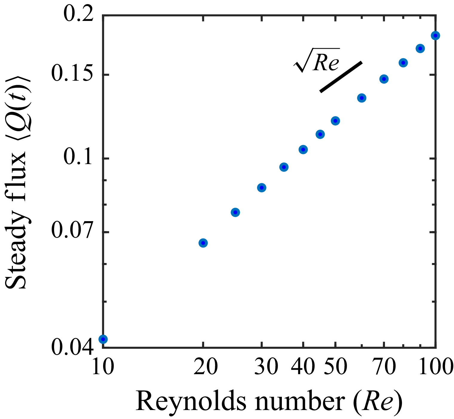
 ϵ=0.5
ϵ=0.5 α=2
α=2 T=300
T=300 32×8
32×8 Re
Re
 32×8
32×8 ϵ=0.5
ϵ=0.5 T=300
T=300 α=1
α=1 α=2
α=2 Re=10
Re=10 Re=50
Re=50
 ψ2=f(r)sin(2θ)
 ψ3(1)=f(r)sin(θ)
 ψ3(3)=f(r)sin(3θ)
 f(r)
f(r) ψ=ϵ2f(r)sin(2θ)+ϵ3f(r)sin(3θ)+ϵ3f(r)sin(θ)
 ϵ=0.45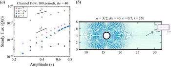
 α=2
α=2 3/2
3/2 4
4 3
3 α=3/2
α=3/2 0.7
0.7 40
40 10
10 10
10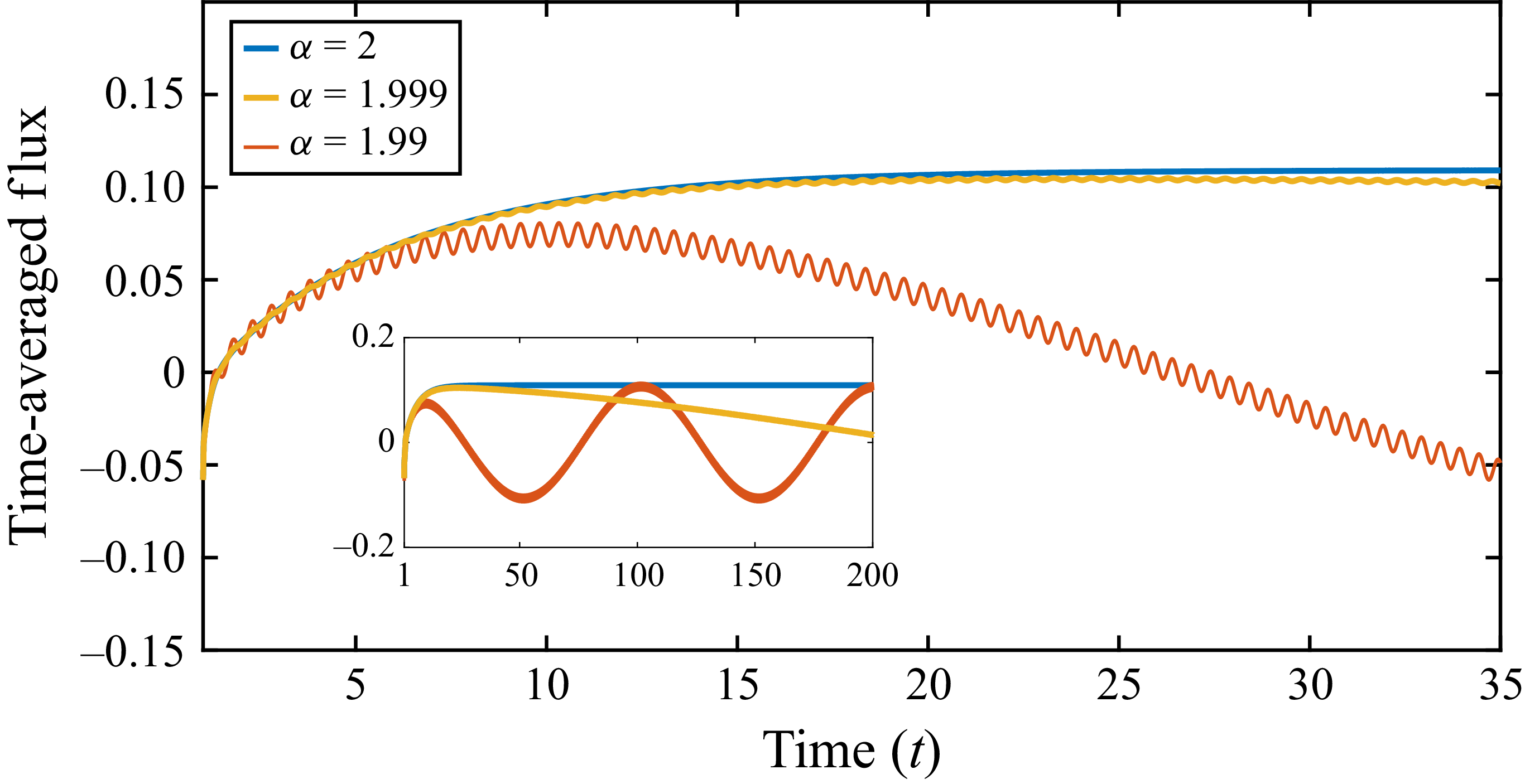
 α=2
α=2 ϵ=0.7
ϵ=0.7 Re=10
Re=10 200
200 α=1.99
 1.999
1.999 α=2
α=2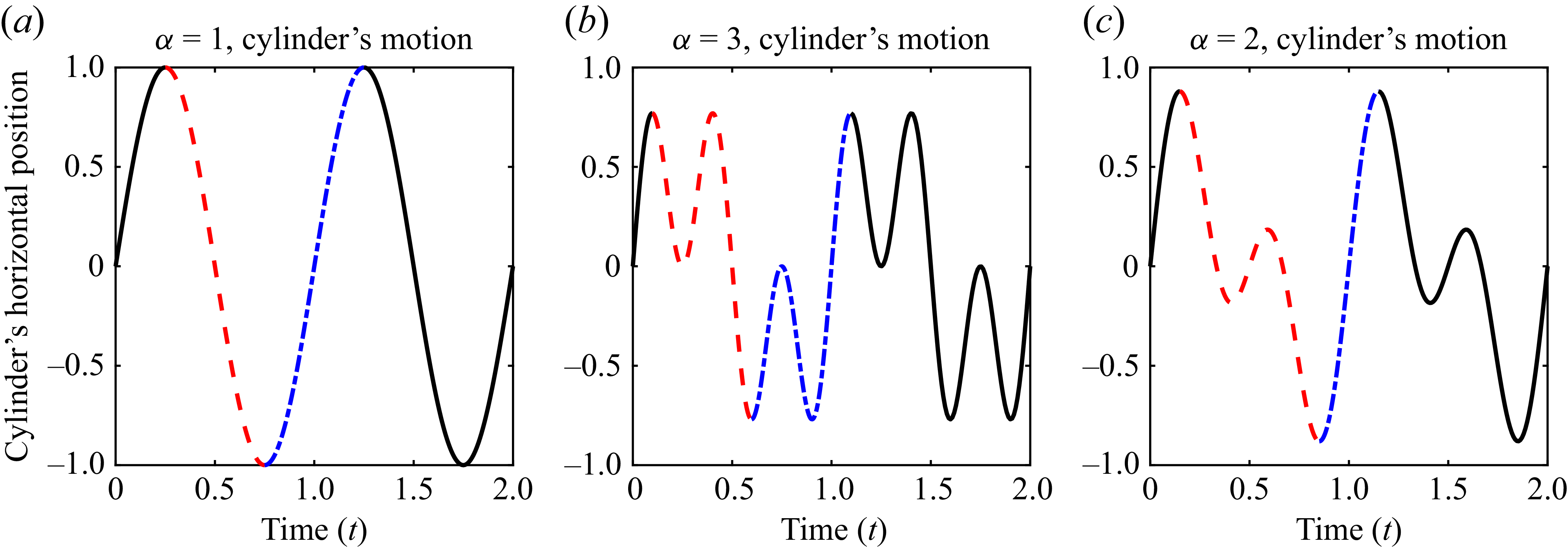
 0≤t≤2
0≤t≤2 α=1
α=1 α=3
α=3 α=2
α=2 A=1
A=1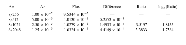
 8×8
8×8 Re=10
Re=10 ϵ=0.5
ϵ=0.5 T=100
T=100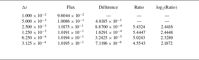
 Δx=8/256
 8×8
8×8 Re=10
Re=10 ϵ=0.5
ϵ=0.5 T=100
T=100


 Open access

