Introduction

While mountain glaciers make up only ∼0.5% of the global land surface they are currently the major land-ice contributors to global sea-level rise (IPCC, 2013). Further, many alpine glaciers are located near human habitations and significantly influence local water supplies. For example, changes in the supply of meltwater produced by mountain glaciers of the Tibetan Plateau could impact as many as 1.3 billion people living downstream (Reference Immerzeel, Van Beek and BierkensImmerzeel and others, 2010). Though in situ and remote-sensing-based observations of glacier changes are being continuously carried out, they can only provide information on past or present-day changes. To predict future mountain glacier changes and their associated impacts, glacier evolution under future climates must be studied with reliable numerical ice-flow models.

Choosing an appropriate glacier model is not a simple matter: computational cost must be balanced against accuracy, and a highly accurate, expensive model may not be justified in the absence of adequate data constraints. Since the 1950s, a number of mathematical ice-flow models have been proposed, such as the shallow-ice approximation (SIA; Reference HutterHutter, 1983; Reference MorlandMorland, 1984), the shallow-shelf approximation (SSA; Reference MorlandMorland, 1987), the so-called ‘higher-order (HO)’ or ‘first- order (FO)’ model (a first-order accurate approximation to the Stokes equations; Reference BlatterBlatter, 1995; Reference PattynPattyn, 2002, Reference Pattyn2003), the L1L2 model (Reference Schoof and HindmarshSchoof and Hindmarsh, 2010; Reference GoldbergGoldberg, 2011; Reference CornfordCornford and others, 2013) and so-called ‘hybrid’ models (a combination of the SIA and SSA; e.g. Reference Bueler and BrownBueler and Brown, 2009). All are based on some approximation to the ‘full’, nonlinear Stokes equations, which have themselves recently been incorporated into large-scale models (Reference Larour, Morlighem, Seroussi, Schiermeier and RignotLarour and others, 2012; Reference Leng, Ju, Gunzburger, Price and RinglerLeng and others, 2012; Reference GagliardiniGagliardini and others, 2013), and have been used in studies of glacier and ice-sheet dynamics (e.g. Reference HuybrechtsHuybrechts, 1990; Reference Saito, Abe-Ouchi and BlatterSaito and others, 2003; Reference Aschwanden and BlatterAschwanden and Blatter, 2005; Reference Gagliardini, Cohen, Råaback and ZwingerGagliardini and others, 2007; Reference Price, Waddington and ConwayPrice and others, 2007; Reference Seddik, Greve, Zwinger, Gillet-Chaulet and GagliardiniSeddik and others, 2012; Reference Leng, Ju, Gunzburger and PriceLeng and others, 2014a).

Because of high-elevation alpine terrain and poor accessibility, geometry datasets for mountain glaciers are generally based on sparse data. This is particularly true for glaciers of the Tibetan Plateau where, for example, nearly all the in situ ice thickness data of the Himalayan East Rongbuk Glacier (∼12 km long) are located along its central flowline (CL), ∼6 km of which is currently unsurveyed (Reference Zhang, Xiao, Qin, Hou and DingZhang and others, 2012, Reference Zhang2013). Three-dimensional (3-D) models may not be the best choice for modelling the dynamics of these glaciers, due to large uncertainties in glacier geometry, and, as a result, 2-D glacier models are widely used for studies in these areas (Reference OerlemansOerlemans, 1986, Reference Oerlemans1997; Reference Aschwanden and BlatterAschwanden and Blatter, 2005; Reference Pattyn, Nolan, Rabus and TakahashiPattyn and others, 2005; Price and Walder, 2007; Reference Adhikari and HuybrechtsAdhikari and Huybrechts, 2009; Reference Pimentel, Flowers and SchoofPimentel and others, 2010; Flowers and others, 2011; Reference ZhangZhang and others, 2013). Mountain glaciers are generally much narrower, and have much larger aspect ratios than ice sheets, in which case the 2-D shallow-ice and plain strain (‘flowline’) approximations (e.g. Reference Cuffey and PatersonCuffey and Paterson, 2010) may not apply. A standard approach is to apply a flowline model, but to adjust velocities along the CL using a ‘shape factor’ (Reference NyeNye, 1965; Reference OerlemansOerlemans, 1986; Reference Pattyn, Nolan, Rabus and TakahashiPattyn and others, 2005; Reference Adhikari and MarshallAdhikari and Marshall, 2012), which applies a correction (generally to the driving stress) to capture the influence of lateral drag from valley walls (Reference NyeNye, 1965). Another approach, which we do not discuss further here, is to parameterize the lateral drag in 2-D ice-flow models using observed glacier width variations (Reference Pimentel, Flowers and SchoofPimentel and others, 2010; Flowers and others, 2011; Reference ZhangZhang and others, 2013).

To date, few studies of mountain glaciers have included the effects of polythermal ice or have explored the importance of thermomechanical coupling. Using the EISMINT-1 geometry and environmental forcings (Reference Huybrechts and PayneHuybrechts and others, 1996), Reference PattynPattyn (2002) tested the transient behaviors of a 2-D FO model without coupling to the temperature field. A more rigorous investigation of higher-order ice-flow models, including applications to a realistic mountain glacier geometry, was carried out during the Ice Sheet Model Intercomparison Project for Higher-Order Models (ISMIP-HOM) (Reference PattynPattyn, 2008). However, the effects of thermomechanical coupling were not considered. Recently, Reference Adhikari and MarshallAdhikari and Marshall (2011, Reference Adhikari and Marshall2012) tried to improve the flowline model based on the SIA by parameterizing the effects of longitudinal-stress coupling and by examining shape factors for different types of glacier troughs, under both sliding and frozen bed conditions. Again, no temperature coupling was incorporated. Due to a lack of temperature observations, Reference Adhikari and MarshallAdhikari and Marshall (2013) assumed a spatially uniform and constant flow law parameter, and concluded that higher-order stresses do not significantly alter the dynamics of Haig Glacier, Canada.

Because isothermal model assumptions may introduce uncertainties when applied to polythermal glaciers (e.g. those of the Tibetan Plateau), the following questions arise: (1) How do the velocity biases in 2-D flowline models influence the englacial temperature field? (2) What is the role of temperature coupling in glacier dynamics for both 2-D diagnostic and prognostic experiments? To address these questions, we explore the impacts of (1) glacier geometry, (2) ice temperature and (3) model integration time on ice-flow dynamics of land-terminating glaciers. We use a 2-D, thermomechanically coupled FO flowline model (FLM) and compare the results with a 3-D, thermomechanical, ‘full’-Stokes model (FSM), under identical conditions of glacier geometry, environmental forcing and boundary/initial settings. For our idealized test cases there are no observations available for use in model validation. Thus, implicit in our comparison is the assumption that solutions from the 3-D FSM are as close as possible to the ‘truth’.

The paper is organized as follows: We first briefly describe the FLM and FSM used in this study. We then present a detailed description of three different experiments designed to test model sensitivities to glacier geometry, ice temperature and model integration time. We then analyze experimental results for each model, in order to comprehensively identify conditions under which FLMs provide reliable results relative to FSMs.

Model Descriptions

Detailed descriptions of the FSM and the FLM used in this study are given by Reference Leng, Ju, Gunzburger, Price and RinglerLeng and others (2012, Reference Leng, Ju, Gunzburger and Price2014a,b) and Reference Greve and BlatterGreve and Blatter (2009), respectively. Verification of the FSM is discussed in detail by Reference Leng, Ju, Gunzburger and PriceLeng and others (2013).

The conservation of momentum for ice flow can be described by

(1)

where σ is the full stress tensor, ρ is the density of ice and g is the acceleration due to gravity. We note that g = (0, 0, g) for the FSM and (0, fg) for the FLM. The tensors, σ, are represented by the 3-D tensor for the FSM and the 2-D tensor for the FLM. The shape factor, f , is used as a correction to the body force in the FLM to parameterize the effects of drag against valley side-walls (e.g. Reference Adhikari and MarshallAdhikari and Marshall, 2012). Glacier ice is generally considered an incompressible material so that

(2)

where u denotes the ice velocity vector, given by (u, v, w) and (u, w) for the FSM and the FLM, respectively.

The deviatoric stress is given by τ = σ + pI , where p is the isotropic ice pressure (p = −tr(σ)/3) and I is the identity matrix. The deviatoric stress is related to the strain-rate tensor, , through a constitutive law,

(3)

Glen’s flow law (Reference Cuffey and PatersonCuffey and Paterson, 2010) and Eqn (3) can be combined to define the ‘effective’ ice viscosity, η, as

(4)

where n is the flow law exponent, A is the temperature-dependent rate factor and is the effective strain rate

(5)

A is described by an Arrhenius-type relation

(6)

with A ₀ a reference flow law parameter, Q the creep activation energy of ice, R the universal gas constant and T the ice temperature (in kelvin). Note that for the FLM, the horizontal derivatives of vertical velocity are neglected in the strain-rate computation (Reference Greve and BlatterGreve and Blatter, 2009). Here the FLM is verified by comparing model output with other FO models described by Reference PattynPattyn (2008) (Fig. 1).

Fig. 1.

Verification of the FLM. FLMa and b denote surface velocities from the FLM using a horizontal grid spacing of 20 and 100 m, respectively. Other first-order model results (ahu1, bds1, fpa1 and mbr1) shown are taken from Reference PattynPattyn (2008).

Conservation of energy is expressed through the advective–diffusive heat equation,

(7)

where k is the conductivity and c the heat capacity of ice (taken as constants here). The pressure-melting point of glacier ice, T _pmp, is described by the Clausius–Clapeyron relation,

(8)

where T ₀ is the triple point of water, s is the ice surface elevation, γ is the Clausius–Clapeyron constant and z is the vertical coordinate. In the models used in this study T is set to satisfy the constraint

(9)

While the ice temperature is allowed to evolve in some experiments, we do not evolve the glacier geometry over time in the present work. By holding the ice geometry fixed, we can conduct grid-to-grid comparisons between the FSM and the FLM, which simplifies our understanding of the impact and importance of thermomechanical coupling (details can be found in the ‘Experiment design’ and ‘Discussion’ sections, below). Because we do not evolve the glacier geometry in time we do not present or discuss the mass-continuity equation here.

Boundary conditions

We assume a stress-free boundary condition at the upper-ice surface,

(10)

where n is the surface normal vector.

At the lower-ice surface (i.e. the ice/bedrock interface), we set the ice velocity to zero if the ice is frozen (T < T _pmp),

(11)

and, if ice temperature reaches the pressure-melting point, T = T _pmp, we apply a linear sliding law (cf. Reference Schoof and HewittSchoof and Hewitt, 2012):

(12)

(13)

where β is a positive sliding parameter and t is the lower-ice surface tangential vector. In the FLM, for numerical stability and ease of implementation we approximate this sliding law (Eqns (12) and (13)) as

(14)

similar to the approach used by Reference Pimentel, Flowers and SchoofPimentel and others (2010).

For the temperature model, we set T equal to the mean annual surface air temperature, T _s, at the upper-ice surface. For generality, we specify these according to

(15)

where γ _e is the environmental lapse rate and T _t and s _t represent the surface air temperature and elevation at the glacier terminus, respectively. The Neumann temperature boundary condition at the ice/bedrock interface is given by

(16)

where G is the geothermal heat flux.

All model constants discussed in this section are summarized in Table 1.

Table 1.

Parameters used in the numerical models

Experiment Design

The FSM and FLM are implemented using finite-element and finite-difference methods, respectively. To facilitate model intercomparisons, we use a layered grid for the FSM with tetrahedral-type elements: the 3-D grid is vertically extruded from a 2-D structured triangle mesh (see Reference Leng, Ju, Gunzburger, Price and RinglerLeng and others, 2012, for further details). For the FLM, we use terrain-following coordinates: (z ∊ [0, 1]; Reference Greve and BlatterGreve and Blatter, 2009). We compare the horizontal velocity component, u, and ice temperature, T, along the CL of the FSM (u _FSM, T _FSM) and the FLM (u _FLM, T _FLM) and compute their percentage relative errors using the following error metrics (the FLM data are first linearly interpolated onto the same grid as for FSM):

(17)

(18)

The relative errors between the FLM and FSM solutions are used to identify conditions under which the FLM approximation becomes a poor approximation of the ‘true’ solution, which we take here as that given by the FSM.

In both models, we apply a Picard iteration for treating the nonlinearity associated with the ice viscosity. Following Reference GagliardiniGagliardini and others (2013), we set the Picard iteration convergence criterion as

(19)

where l denotes the iteration step.

A comprehensive evaluation of the FLM for use on polythermal, mountain glacier dynamics is afforded by examining the distribution of the error metrics, r_u and r_T , as a function of ice geometry (e.g. length, slope, width, bedrock topography), temperature and model integration time. Three numerical experiments are designed as follows (Table 2).

ESD: Experiments for steady-state, thermomechanically decoupled models. Similar to the EISMINT-I experiments (Reference Huybrechts and PayneHuybrechts and others, 1996), we first diagnose the velocity field using a constant and uniform flow law parameter, A = 10⁻¹⁶ Pa⁻³ a⁻¹, and then use this velocity field for computing a temperature field. Thus, while we calculate both the velocity and temperature distributions, they are not coupled through the calculation of the flow law rate factor. For both the FSM and FLM models, we use the Haut Glacier d’Arolla (Switzerland) CL geometry (hereafter referred to as HGA; Reference PattynPattyn and others, 2008) with a uniform width of 1 km (ESD-1). To isolate the impact of different geometric parameters, we also model the flow within several idealized ice geometries, for example, three ‘ice-slab’ geometries (uniform surface slope and ice thickness) and two idealized geometries with Gaussian bumps along the bed. For the slab geometries, we vary the length, L (2, 4 and 8 km; ESD-2), surface slope, α (0.1, 0.2 and 0.3; ESD-3), and glacier width, W (0.4, 1.2 and 2.0 km; ESD-4). For all ice-slab model experiments, the ice thickness, H, is set to 100 m and a velocity boundary condition of u = 0 is applied at the glacier head and terminus. To improve our understanding of the impact of extensive and compressive ice flow, we further consider slab geometries (4 km long and 1.2 km wide with a surface slope of 0.2) with perturbed concave (ESD-5; M = −10, −20, −40 m) or convex (ESD-6; M = 10, 20, 40 m) Gaussian bumps along the bedrock,

(20)

where b is the bedrock elevation. Using the Gaussian bump geometries, we analyze the relative importance of pure advection and pure diffusion on the ice temperature fields between the FSM and the FLM. In ESD-1–6, we set T _t = 268.15 K, which results in a frozen ice/bed interface.

ESC: Experiments for quasi-steady-state, thermomechanically coupled models. Using the fixed HGA geometry, we set ∂T=∂t to zero in Eqn (7) and recalculate A(T) at every step after the velocity field is computed. Thus, for each iterative velocity solution, we calculate a corresponding steady-state temperature field. The thermomechanically coupled model runs until the u and T fields are converged. To study flow regimes with both frozen and thawed (i.e. sliding) beds, we set the surface temperature at the terminus, T _t, to be 268.15 K (ESC-1) and 276.15 K (ESC-2) for cold and polythermal glaciers, respectively. In the case of a thawed bed, we test the model sensitivity by varying the sliding law parameter between β = 2 × 10⁴ Pa a m⁻¹ (ESC-3) and β = 4 × 10⁴ Pa a m⁻¹ (ESC-4).

ETC: Experiments for transient, thermomechanically coupled models. Like the ESC experiments, we again use the fixed HGA geometry. However, for these experiments we include the ∂T=∂t term in the temperature calculation and let it freely evolve. Two model run durations, 100 and 1000 years, are studied for both frozen and thawed (sliding) basal conditions. We use ETC-1–4 to denote experiments with the parameter pairs (t _end = 100 years, T _t = 268.15 K), (t _end = 1000 years, T _t = 268.15 K), (t _end = 100 years, T _t = 276.15 K) and (t _end = 1000 years, T _t = 276.15 K), respectively. The initial temperature fields for both the FSM and FLM are steady-state solutions taken from a purely diffusive temperature model (i.e. without heat advection) under the same boundary conditions as noted above.

Table 2.

Details of numerical experiments. CLG: geometry along the center flowline (CGB: slab with concave Gaussian bump; VGB: slab with convex Gaussian bump). CST: cross-sectional type (R: rectangular; U: parabolic)

Note that in the experiments above, both the FSM and the FLM have identical central flowline geometry and a horizontal grid size of 100 m. For the FSM, we use six vertical layers, which, because the FSM uses high-order finite elements (Reference Leng, Ju, Gunzburger, Price and RinglerLeng and others, 2012), provide a level of accuracy nearly identical to that when using far more (e.g. 21) vertical layers. For the FLM, there are two different situations: (1) for the experiments with HGA geometry, we use 51 vertical layers; (2) for the experiments with slab and Gaussian bump geometries, we choose the vertical layer number (∼20–40) by comparing the modelled FLM and FSM velocity fields for the infinitely long and wide geometries. In other words, the number of vertical layers used for the FSM and the FLM are chosen to optimize both model performance and accuracy and to minimize differences imparted because of differing grids. The glacier cross section for HGA is assumed to be parabolic, but for ice-slab and Gaussian bump cases we set rectangular cross sections, so that we can apply periodic boundary conditions along the x-direction for the FLM and along both the x- and y-directions for the FSM. The corresponding shape factor values (see Reference Adhikari and MarshallAdhikari and Marshall, 2012) are linearly interpolated as a function of x. The geothermal heat flux is set to be uniform over the entire model domain. For the convenience of model comparisons, we simply constrain temperate ice to be not greater than T _pmp for both the FSM and FLM, noting that this may bias model results in the cases of real glaciers (Reference Zwinger, Greve, Gagliardini and ShiraiwaZwinger and others, 2007).

Model Results

Results for steady-state, thermomechanically decoupled experiments (ESD)

Shape factors are obtained from numerical experiments using infinitely long ice-slab geometries (Reference NyeNye, 1965; Reference Adhikari and MarshallAdhikari and Marshall, 2012). In reality, however, glaciers have finite lengths and longitudinal velocity gradients may also have a non-negligible impact on ice flow. In addition, the hydrostatic and first-order approximation that the FLM is based on will also lead to model errors. Thus, relative to simulations using the FSM, we expect biased results when using the FLM combined with a shape factor to parameterize the effects of lateral drag, σ_xy .

Such a bias can be observed in Figure 2. For HGA (ESD-1), the FLM produces smaller u values in general and also underestimates the values of T near the ice base, both of which can be largely attributed to ice geometries, as demonstrated by the ice-slab and Gaussian bump model experiments (Fig. 3). In ESD-2–6 , the model sensitivities to glacier length, slope, width and Gaussian bump geometries are studied. From these experiments we find that different geometries result in different levels of velocity underestimation for the FLM, which is partly a result of approximations inherent to the FLM. In order to calculate the model error, r_{u m} (as a result of the FLM approximations), we carry out experiments with no lateral drag (f = 1) so that r_{u m} = r_u . r_{u m} is very sensitive to ice slopes and bedrock undulations (Fig. 3; ESD-3, 5 and 6).

Fig. 2.

ESD model results for the HGA geometry with parabolic cross sections: (a) r_u distribution; (b) r_T distribution; (c) surface, u _s, and basal, u _b, velocity of the FSM and the FLM along the CL; (d) difference of the mean column ice temperature between FSM and FLM () along the CL.

Fig. 3.

Experiments ESD-2–6 with rectangular cross sections (for different glacier lengths, slopes, widths, concave Gaussian bumps and convex Gaussian bumps; Table 2). Each subplot contains two parts: (bottom) surface velocity distribution along the CL. The blue and red curves are for the FSM and FLM, respectively, while the solid and dashed curves are for experiments with lateral drag and without lateral drag (shape factor equal to 1), respectively; (top) the corresponding errors, r_{u m}, due to model simplifications, shown by the thick, solid blue curve.

Errors in the velocity field, u, result in errors in the corresponding equilibrium T field. With a frozen bed, the FLM generally produces smaller ∂u=∂z values near the glacier base, and hence less shear heating. Also, the FLM retains only the and terms, while neglecting all other terms in the calculation of strain heating. Therefore, we hypothesize that the FLM results in relatively ‘cooler’ ice temperatures for most parts of the HGA domain.

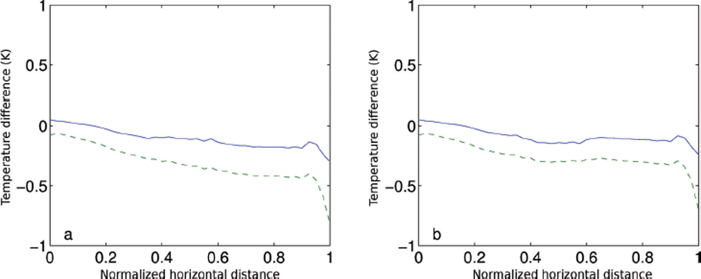
Before exploring this further, we first confirm that the two temperature models give comparable results. As shown in Figure 4, the temperature results of the FSM (with periodic boundary conditions along the y-direction) compare well with those from the FLM (f = 1) when using the same velocity field, which in both cases is taken from the FSM (blue solid curve in Fig. 4). Based on this analysis, we assume that temperature differences between the FLM and the FSM, resulting from the different model discretizations, are minor.

Fig. 4.

Verification of the FLM temperature model. Shown are steady-state temperature differences when using (a) concave (M = −10 m) and (b) convex (M = 10 m) Gaussian bump geometries with rectangular cross sections. The curves represent the difference of the mean ice column temperature along the CL between the FSM and the FLM (). The solid blue curve shows differences when both temperature models use the velocity field from the FSM. The dashed green curve shows differences when each model uses its own velocity field.

We next conduct a series of experiments where either the viscous dissipation or the advection components are switched ‘off’ in the calculation of the temperature in both the FLM and the FSM (Fig. 5). Without dissipative heating, we find that the FLM produces a slightly warmer ice (relative to the FSM), as a result of its slightly less advection of cold ice (red curves, Fig. 5). However, we can see that temperatures from the FLM are much cooler relative to the FSM in the absence of advection, when only the dissipative heating and diffusion terms act (blue curves, Fig. 5), indicating that, overall, the larger velocities of the FSM act to warm the ice rather than cool it (relative to the FLM). As a consequence, compared to the FSM, the FLM leads to generally cooler temperatures, especially near the bed, where the FLM underestimation of ∂u/∂z is large. We attribute the generally ‘cool’ bias of the FLM, shown by the green dashed curves in Figure 4, to this same mechanism.

Fig. 5.

The contributions of viscous heat dissipation and advection are studied using (a) concave (M = −10 m) and (b) convex (M = 10 m) Gaussian bump geometries without lateral drag (f = 1). The lower and upper figure panels show the mean column temperature profiles of FSM (solid curves) and FLM (dashed curves) and their relative errors along the central flowline, respectively. The blue, black and red curves represent temperature models without advection, complete temperature models and temperature models without viscous heat dissipation, respectively.

Results for quasi-steady-state, thermomechanically coupled experiments (ESC)

For the case of cold glaciers (ESC-1; Fig. 6), when coupled through the rate factor, the FLM generally produces additional biases in u, but there is no clear and consistent pattern whereby temperature and dynamical coupling increases or decreases the temperature biases between the FLM and the FSM: different geometries in different parts of a glacier may lead to different ice dynamics, different velocity and temperature fields, and different feedbacks between the two.

Fig. 6.

ESC-1 model results for the HGA geometry with parabolic cross sections: (a) r_u distribution; (b) r_T distribution; (c) surface, u _s, and basal, u _b, velocity of FSM and FLM along the CL; (d) difference of the mean column ice temperature between FSM and FLM () along the CL.

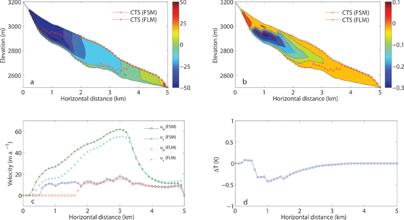
However, the results of the polythermal glacier experiment (ESC-2), in which basal sliding is allowed, are remarkably different. Both the u and T fields differ significantly when a temperate ice zone (TIZ) forms (Fig. 7). Compared with the FLM, the FSM produces a more extensive TIZ. Figure 7 shows that the largest differences between the modelled u and T occur between the cold/ temperate ice transition surfaces (CTSs). A likely cause for these differences is the presence or absence of basal sliding: since the FSM produces warmer basal ice (as discussed above) it is more likely that temperate ice appears closer to the head of the glacier relative to the FLM when the TIZ size increases. Once temperate ice appears upstream, the ice downstream of it is also more likely to be temperate, through the downstream advection of temperate basal ice, through enhanced viscous heat dissipation (afforded by more rapid deformation in soft basal ice) and through frictional heating generated by sliding (as illustrated in Fig. 8a). For the FSM (FLM), temperate (cold) ice is transported from upstream to downstream faster as a result of sliding, with the result that the CTS positions predicted by the two models are very different in the presence of sliding (Fig. 8a). Conversely, in the absence of sliding, the CTS positions predicted by the two models are much more comparable (Fig. 8a). We can find additional evidence for this mechanism in ESC-3 and 4, for which we set the basal sliding parameter, β, to 2 × 10⁴ and 4 × ⁴ Pa a m⁻¹ (Fig. 8b), respectively. This change leads to changes in the extents of the TIZs for the FSM and the FLM, which become more similar (their sizes are still greatly different), relative to ESC-2 (β = 1 × 10⁴ Pa a m⁻¹), when β increases (sliding velocity decreases) (Fig. 8b).

Fig. 7.

ESC-2 model results for the HGA geometry with parabolic cross sections: (a) r_u distribution (absolute values >50% are not shown); (b) r_T distribution; (c) surface, u _s, and basal, u _b, velocity of FSM and FLM along the CL; (d) difference of the mean column ice temperature between FSM and FLM () along the CL. CTS represents the cold/temperate ice transition surface.

Fig. 8.

Comparison of the cold/temperate ice transition surface (CTS) positions of FSM (blue curves) and FLM (red curves). (a) The solid and dashed curves represent the cases in which basal sliding is allowed and prohibited, respectively. (b) The thick solid curves, the curve with circles and the curve with crosses are for the sliding parameter β =1 × 10⁴, 2 × 10⁴ and 4 × 10⁴ Pa a m⁻¹, respectively (for the FSM, those three curves nearly overlap). The cross-sectional type is parabolic.

Results of transient, thermomechanically coupled model experiments (ETC)

To study the impact of model integration time on the differences between the FLM and the FSM, we integrate the thermomechanically coupled models forward in time while holding the domain geometry fixed (as discussed above). For the case of both frozen (no slip) and thawed (sliding) beds, we examine model differences at time steps associated with 100 and 1000 years of forward integration (Figs 9 and 10, respectively). At the beginning of the transient modelling, the temperature fields of both the FSM and FLM are initialized with pure heat diffusion (u = 0) under the same boundary (geothermal heat flux and surface air temperature) settings.

Fig. 9.

ETC-1 (100 years of integration) and ETC-2 (1000 years of integration) model results for the HGA geometry with parabolic cross sections. (a, c) surface, u _s, and basal, u _b, velocity of FSM and FLM along the CL. (b, d) Difference of the mean column ice temperature between FSM and FLM () along the CL.

Fig. 10.

ETC-3 (100 years of integration) and ETC-4 (1000 years of integration) model results for the HGA geometry with parabolic cross sections. (a, c) surface, u _s, and basal, u _b, velocity of FSM and FLM along the CL. (b, d) Difference of the mean column ice temperature between FSM and FLM () along the CL.

As might be expected, we find that the discrepancies between the FLM and FSM u and T fields become larger over time, relative to results of the ESC experiments. For example, the |r_u | of ETC-2 is greater than that of ETC-1 in most parts of HGA (Fig. 9). This indicates that biases between the FLM and the FSM, in both the u and T fields, grow over time, presumably through the feedback between u and T in Eqn (7). This feedback becomes even more important when the glacier is sliding, whereby the FLM versus FSM discrepancies between the u and T fields at integration times of 100 versus 1000 years become even larger (Fig. 10). A small initial difference in the FLM and FSM T fields is magnified through the thermomechanical feedbacks discussed above, such that the final extent of the TIZs in the two models is markedly different.

Discussion

In addition to the experiments discussed in detail above, we conducted model experiments using different cross-sectional shapes (rectangular rather than parabolic), using other longitudinal ice geometries (the simple analytic glacier profile presented by Reference Le Meur, Gagliardini, Zwinger and RuokolainenLe Meur and others, 2004, and Reference Adhikari and MarshallAdhikari and Marshall, 2012, as opposed to the HGA geometry), and using different grid resolutions. The conclusions from these additional experiments are qualitatively similar to those described above. Real glaciers, however, have sufficiently complex and spatially varying geometries that render it impossible to conduct an exhaustive and conclusive series of experiments for more-realistic glaciers. For example, the index of the power law function that describes cross-sectional shapes (2 for parabolic cross sections) will vary spatially over a wide range for real glaciers. Further, glacier cross sections are often highly unsymmetric (e.g. Reference Zhang, Xiao, Qin, Hou and DingZhang and others, 2012) and glacier widths are not uniform along flow (as assumed in this study). Therefore, we expect that additional errors and biases of the sort demonstrated here can be expected when applying a FLM to approximate the evolution of realistic, 3-D glaciers.

Reference Adhikari and MarshallAdhikari and Marshall (2012) argued that two types of correction factors induced by glacier geometry, f _n, and sliding conditions, f _s, should be accounted for (f = f _n × f _s). In this study, we included only f _n (f = f _n), as it would not be practical to implement f _s during the model numerical iterations and to distinguish between ‘abrupt’ and ‘smooth’ basal sliding transition regions. While we expect that the additional factor f _s (<1) could further reduce the values of u in the FLM relative to the FSM (thus resulting in even larger discrepancies between the FSM and FLM results) and that different basal sliding ‘laws’ (e.g. Weertman-type (Reference Cuffey and PatersonCuffey and Paterson, 2010) or Coulomb- friction type (Reference Gagliardini, Cohen, Råaback and ZwingerGagliardini and others, 2007)) may introduce additional differences, our conclusion that basal sliding will enhance biases between the FLM and FSM should be robust.

While we have studied model sensitivities with respect to integration time in this paper, we have not carried out any prognostic simulations whereby the glacier geometry is allowed to change over time. Here this is because a comparison of ice-volume changes between the FSM and the FLM is far from straightforward. The u profiles along glacier cross sections are not well understood (e.g. Reference NyeNye, 1965), but for modelling volume evolution using a FLM a reliable parameterization of the mean, across-flow ice flux is required at each point along flow. In general, it is not clear how best to conduct a fair and meaningful comparison of glacier geometry changes as calculated by the FLM with those calculated by the FSM.

Conclusions

By comparing output from a 3-D, thermomechanical, full-Stokes model (FSM) and a 2-D, thermomechanical, first-order flowline model (FLM) we investigated model sensitivities to three different factors: glacier geometry (e.g. length, slope, width and bed undulation), ice temperature and model integration time. We find that, in common situations, the FLM will be heavily biased and should therefore be used and interpreted with caution. These situations include the simulation of (1) glaciers that are steep and with heavily undulated bed topography, (2) polythermal glaciers for which there is a temperate basal ice zone and for which basal sliding occurs and (3) glacier evolution over long time periods (∼10³ years). Put differently, the FLM is more likely to give accurate results (relative to a FSM) for flat, cold or temperate glaciers with relatively short equilibrium timescales (i.e. less than several hundred years).

Among the factors tested here, we argue that the glacier geometry (accounted for in part by the shape factor for the FLM) is likely to lead to the biggest differences in simulation outputs for the FLM versus the FSM. While the presence or absence of basal sliding leads to the largest overall model differences, this is largely a result of differences in the modelled temperature fields. These originally arise from small differences in the modelled ice velocity fields, which grow over time through positive, thermomechanical feedbacks. In turn, these initially small differences in the velocity field arise because of approximations inherent to the FLM and the way that geometry is parameterized in the FLM (i.e. using a shape factor to parameterize the effects of lateral drag).