


1. Introduction
Thermal convection at low Prandtl numbers is a common phenomenon both in nature and in many engineering applications. Here, the Prandtl number is defined as  $Pr=\nu /\kappa$, it represents the relative importance of the kinematic viscosity $\nu$ to the thermal diffusivity $\kappa$ of the convecting fluid. For example, astronomical observations showed that the Sun has an outer convecting layer of low-density plasma, where the value of $Pr$ is in the range of $10^{-7}$– $10^{-4}$ (Hanasoge, Gizon & Sreenivasan Reference Hanasoge, Gizon and Sreenivasan2016; Schumacher & Sreenivasan Reference Schumacher and Sreenivasan2020). Seismology measurements showed that the outer core of the Earth is a fluid layer made of a liquid iron–nickel alloy with $Pr\sim 10^{-2}$ (Stevenson Reference Stevenson1981). The convection of the Earth's outer core is linked to the generation and reversal of the Earth's magnetic field (Glatzmaier & Roberts Reference Glatzmaier and Roberts1995). The convection of the Earth's atmosphere with $Pr\simeq 0.7$ drives the large-scale atmospheric circulation and plays a critical role in the global climate and water balance (Hartmann, Moy & Fu Reference Hartmann, Moy and Fu2001). Liquid-metal convection is also used in material processing (Brodova, Popel & Eskin Reference Brodova, Popel and Eskin2001), nuclear engineering (Ihli et al. Reference Ihli2008), and liquid-metal batteries for renewable energy storage (Wang et al. Reference Wang2014).
In the laboratory, controlled Rayleigh–Bénard convection (RBC) experiments are conducted in a closed cell, in which a fluid layer is heated from below and cooled from above. In addition to the Prandtl number  $Pr$, the Rayleigh number $Ra$ is another control parameter of thermal convection, which is defined as $Ra=g\alpha \Delta TH^3/(\nu \kappa )$, where $g$ is the gravitational acceleration, $\alpha$ is the thermal expansion coefficient of the fluid and $\Delta T$ is the temperature difference across the fluid layer of height $H$. When the Rayleigh number is sufficiently large (e.g. $Ra\gtrsim 10^8$ for $Pr\simeq 4.4$), the bulk fluid becomes turbulent and a large-scale circulation (LSC) is formed across the convection cell (Krishnamurti & Howard Reference Krishnamurti and Howard1981; Zocchi, Moses & Libchaber Reference Zocchi, Moses and Libchaber1990). The LSC is driven by the warm and cold plumes emitted from the unstable thermal boundary layers near the bottom and top conducting plates and is maintained in a turbulent environment. This large-scale flow with $Pr>1$ has been studied extensively in upright cylindrical cells of aspect ratio unity (Du & Tong Reference Du and Tong2000; Qiu & Tong Reference Qiu and Tong2001; Xi, Lam & Xia Reference Xi, Lam and Xia2004; Sun, Xia & Tong Reference Sun, Xia and Tong2005), in which the LSC has a single roll structure, with its size comparable to the cell height.
Another intriguing feature of turbulent RBC is that its thermal boundary layer has significant fluctuations resulting from intermittent eruption of thermal plumes from the boundary layer, even when the boundary layer is not fully turbulent (Du & Tong Reference Du and Tong2000; du Puits, Resagk & Thess Reference du Puits, Resagk and Thess2010; Zhou & Xia Reference Zhou and Xia2010). The structure and dynamics of the thermal boundary layer and its interaction with the LSC are of great importance in determining the global heat transport of the system (Kadanoff Reference Kadanoff2001; Ahlers, Grossmann & Lohse Reference Ahlers, Grossmann and Lohse2009). For these reasons, the past decade has witnessed a continuing growth of experimental and theoretical efforts aimed at understanding the boundary-layer dynamics in turbulent RBC. Recent studies of the thermal boundary layer for  $Ra \lesssim 10^{12}$ and $Pr\gtrsim 1$ (Belmonte, Tilgner & Libchaber Reference Belmonte, Tilgner and Libchaber1993, Reference Belmonte, Tilgner and Libchaber1994; Lui & Xia Reference Lui and Xia1998; Du & Tong Reference Du and Tong2000; van Reeuwijk, Jonker & Hanjalić Reference van Reeuwijk, Jonker and Hanjalić2008; Scheel, Kim & White Reference Scheel, Kim and White2012; Shi, Emran & Schumacher Reference Shi, Emran and Schumacher2012; Stevens et al. Reference Stevens, Zhou, Grossmann, Verzicco, Xia and Lohse2012; Wagner, Shishkina & Wagner Reference Wagner, Shishkina and Wagner2012; van der Poel, Stevens & Lohse Reference van der Poel, Stevens and Lohse2013; du Puits, Resagk & Thess Reference du Puits, Resagk and Thess2013; Shishkina, Horn & Wagner Reference Shishkina, Horn and Wagner2013; Zhou & Xia Reference Zhou and Xia2013; Scheel & Schumacher Reference Scheel and Schumacher2014) showed that the measured (and numerically calculated) normalised mean temperature profile $\theta (z)$ has a universal form $\theta (\xi )$, where $\xi \equiv z/\delta _T$ is the vertical distance from the conducting plate normalised by the thermal boundary-layer thickness $\delta _T$. The measured $\theta (\xi )$ was found to be invariant with $Ra$ and has the Prandtl–Blasius–Pohlhausen (PBP) form (Landau & Lifshitz Reference Landau and Lifshitz1987; Schlichting & Gersten Reference Schlichting and Gersten2016) for a laminar boundary layer (Grossmann & Lohse Reference Grossmann and Lohse2000) only when $\xi$ is in the region $\xi \lesssim 0.6$ (Zhou & Xia Reference Zhou and Xia2013). Deviations of $\theta (\xi )$ from the PBP form were found when $0.6 \lesssim \xi \lesssim 4$ (Scheel et al. Reference Scheel, Kim and White2012; Shi et al. Reference Shi, Emran and Schumacher2012; Wagner et al. Reference Wagner, Shishkina and Wagner2012; du Puits et al. Reference du Puits, Resagk and Thess2013). More recently, Shishkina et al. (Reference Shishkina, Horn, Wagner and Ching2015) considered the effect of boundary-layer fluctuations and obtained an analytical form of $\theta (\xi )$ for the thermal boundary layers with $Pr>1$, which explained the observed deviations of $\theta (\xi )$ from the PBP form. The theoretical prediction made by Shishkina et al. (Reference Shishkina, Horn, Wagner and Ching2015) was verified by the convection experiments conducted in a quasi-two-dimensional (quasi-2-D) thin-disk cell (Wang, He & Tong Reference Wang, He and Tong2016). Wang et al. (Reference Wang, Xu, He, Yik, Wang, Schumacher and Tong2018) further extended the boundary-layer theory to the temperature variance profile.
Compared with the large number of investigations on the dynamics of the LSC and boundary layers for  $Pr\gtrsim 1$, our understanding on the LSC and boundary-layer dynamics for fluids with $Pr< 1$ is rather limited. This is partially caused by the fact that laboratory experiments and numerical simulations of turbulent RBC at low $Pr$ are quite challenging. On the experimental side, liquid metals, which are often used as a working fluid to obtain a sufficiently low value of $Pr$, are opaque and thus exclude optical imaging or particle tracking of the velocity field. Owing to their high thermal conductivity, it is also quite difficult to drive the low- $Pr$ convection to reach sufficiently high Rayleigh numbers. On the numerical simulation side, because the Kolmogorov scale in the low- $Pr$ fluid is smaller than the Batchelor scale by a factor of $Pr^{1/2}$ (Grötzbach Reference Grötzbach1983; Shishkina et al. Reference Shishkina, Stevens, Grossmann and Lohse2010), a higher spatial resolution is needed to resolve the smaller Kolmogorov scale for low- $Pr$ convection at a comparable value of $Ra$.
$Ra$.
Early low- $Pr$ experiments using liquid mercury ( $Pr\simeq 0.024$) (Takeshita et al. Reference Takeshita, Segawa, Glazier and Sano1996; Cioni, Ciliberto & Sommeria Reference Cioni, Ciliberto and Sommeria1997; Mashiko et al. Reference Mashiko, Tsuji, Mizuno and Sano2004; Tsuji et al. Reference Tsuji, Mizuno, Mashiko and Sano2005) or gases (such as nitrogen and sulfur hexafluoride) and gas mixtures ( $0.18\leq Pr\leq 0.88$) (Hogg & Ahlers Reference Hogg and Ahlers2013) studied the Nusselt number (normalised heat flux) scaling, thermal boundary-layer profile, LSC dynamics and single-point velocity and temperature statistics in the bulk region. Recent low- $Pr$ experiments using liquid gallium and its alloys ( $Pr\simeq 0.027$) (Vogt et al. Reference Vogt, Horn, Grannan and Aurnou2018; Zürner et al. Reference Zürner, Schindler, Vogt, Eckert and Schumacher2019) investigated the three-dimensional (3-D) structure and dynamics of LSC in the $Ra$ range $10^5\lesssim Ra\lesssim 6\times 10^7$. These experiments found that the LSC at low $Pr$ is more coherent compared with that at high $Pr$ ( $>1$). Recent advances in computational power and numerical techniques allow the study of turbulent RBC at low $Pr$ by direct numerical simulation (DNS) (Schumacher, Götzfried & Scheel Reference Schumacher, Götzfried and Scheel2015; Scheel & Schumacher Reference Scheel and Schumacher2016, Reference Scheel and Schumacher2017; Schumacher et al. Reference Schumacher, Bandaru, Pandey and Scheel2016). It was found that the mean streamwise velocity is like a near-wall jet (Scheel & Schumacher Reference Scheel and Schumacher2017). Many of the experimental and DNS studies were conducted in upright cylindrical cells with an aspect ratio close to unity. In the cylindrical cells, the large-scale flow has several 3-D flow modes, such as the torsional and sloshing modes (Funfschilling & Ahlers Reference Funfschilling and Ahlers2004; Brown & Ahlers Reference Brown and Ahlers2008, Reference Brown and Ahlers2009; Xi et al. Reference Xi, Zhou, Zhou, Chan and Xia2009; Ji & Brown Reference Ji and Brown2020), which may cause additional complications to the study of the LSC and boundary-layer dynamics. There are also corner flows in the closed cylinder (Sun et al. Reference Sun, Xia and Tong2005), which may destabilise the large-scale flow (Sugiyama et al. Reference Sugiyama2010). The strong coupling between the boundary-layer dynamics and complex 3-D large-scale flow in a closed cylinder, which has been studied in recent numerical simulations (van Reeuwijk et al. Reference van Reeuwijk, Jonker and Hanjalić2008; Scheel et al. Reference Scheel, Kim and White2012; Shi et al. Reference Shi, Emran and Schumacher2012; Stevens et al. Reference Stevens, Zhou, Grossmann, Verzicco, Xia and Lohse2012; Wagner et al. Reference Wagner, Shishkina and Wagner2012; van der Poel et al. Reference van der Poel, Stevens and Lohse2013; Shishkina et al. Reference Shishkina, Horn and Wagner2013; Scheel & Schumacher Reference Scheel and Schumacher2014), makes a quantitative comparison between the experiment and 2-D theory difficult.
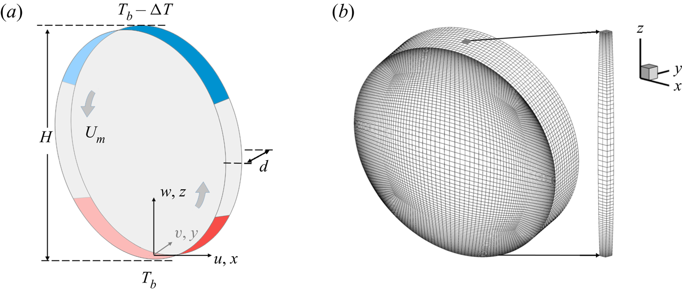
In this paper, we report a systematic numerical study of the mean horizontal velocity profile and mean temperature profile for turbulent RBC in the low- $Pr$ regime. DNS runs were performed in a vertical thin disk with its circular cross-section aligned parallel to gravity (see figure 1 for details). This specially designed quasi-2-D convection cell has two unique features for the DNS study attempted here. First, because the cell shape matches the single-roll structure of the LSC perfectly, there is no corner flow inside the cell. The LSC in the circular cross-section has a steady rotation along a fixed orientation. Owing to the axial symmetry of the thin disk cell, the initial orientation of the LSC is random for different initial conditions and different values of $Ra$. Second, because the flow is confined in a thin circular disk, no 3-D flow modes can be excited in this system. The quasi-2-D flow in the thin disk cell, therefore, has a better geometry satisfying the assumption of the boundary-layer theory for a 2-D flow. Even with these simplifications, the quasi-2-D system retains the key features of turbulent convection, which have been observed in the upright cylinders, and has been used in recent experimental and numerical studies of the LSC dynamics (Song & Tong Reference Song and Tong2010; Song, Villermaux & Tong Reference Song, Villermaux and Tong2011; Song et al. Reference Song, Brown, Hawkins and Tong2014) and thermal boundary-layer profiles with $Pr> 1$ (Wang et al. Reference Wang, He and Tong2016, Reference Wang, Xu, He, Yik, Wang, Schumacher and Tong2018). This is a ‘simple but not simpler’ convection system, which offers a natural platform to study the dynamics of the LSC and boundary layers, and their interactions in the low- $Pr$ regime, and to test different theoretical ideas.
(a) Sketch of the convection cell used for numerical simulations. The convection cell is a vertical thin disk of height  $H$ and thickness $d$. The bottom and top 1/3 of the curved sidewall are made of conducting plates whose temperature is kept at constant with $T_b$ and $T_b-\Delta T$, respectively. All the other walls are thermally insulating. The arrows indicate the direction of the LSC with a maximum velocity $U_m$. The local velocity components and spatial coordinates used in the simulation and data analysis are shown at the bottom centre of the convection cell. (b) A thin column surrounding the vertical $z$-axis of the cell is used to compute the time-averaged properties of the flow as a function of $z$. The horizontal cross-section of the thin column has 4 primary elements and 256 nodes, which form a small area of 0.027 thickness square and are used to calculate the time-averaged properties of the flow.
In this DNS study, we vary the Rayleigh number in the range  $5\times 10^8 \leq Ra \leq 1\times 10^{10}$ and focus our attention on $Pr=0.17$. This is the lowest value of $Pr$ that can be reached by using a gas mixture of H $_2$ and Xe (Bajaj, Ahlers & Pesch Reference Bajaj, Ahlers and Pesch2002), and we choose this value of $Pr$ so that the DNS results can be used for comparison with future experiment. This value of $Pr$ is small enough so that the viscous and thermal boundary layers are well separated with the viscous boundary layer being nested within the thermal boundary layer. In this case, the LSC can produce a strong shear to the thermal boundary layer, which suppresses the emission of thermal plumes from the thermal boundary layer. On the other hand, the value of $Pr$ used is not too small so that we can carry out the DNS study at high Rayleigh numbers with an adequate spatial resolution using the available computational resources.
The remainder of the paper is organised as follows. We first present the numerical method used and DNS set-up in § 2. A comparison of the temperature and velocity fields between the low- $Pr$ and high- $Pr$ regimes is given in § 3. The DNS results of the mean horizontal velocity and temperature profiles in the boundary-layer region are presented in § 4. The DNS results of the mean horizontal velocity profile in the bulk region are presented in § 5. Finally, the findings of this study are summarised in § 6.
2. Direct numerical simulation
The governing equations for turbulent RBC are the incompressible Navier–Stokes equations and the convective heat equation under the Boussinesq approximation. The dimensionless forms of these equations are given by
 \begin{gather} \hat{\boldsymbol{\nabla}}\boldsymbol{\cdot}\hat{\boldsymbol{u}}=0, \end{gather}
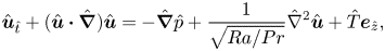 \begin{gather}\hat{\boldsymbol{u}}_{\hat{t}}+(\hat{\boldsymbol{u}}\boldsymbol{\cdot}\hat{\boldsymbol{\nabla}}) \hat{\boldsymbol{u}}={-}\hat{\boldsymbol{\nabla}}\hat{p}+\frac{1}{\sqrt{Ra/Pr}}\hat{\nabla}^2\hat{\boldsymbol{u}} +\hat{T}\boldsymbol{e}_{\hat{z}}, \end{gather}
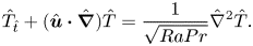 \begin{gather}\hat{T}_{\hat{t}}+(\hat{\boldsymbol{u}}\boldsymbol{\cdot}\hat{\boldsymbol{\nabla}})\hat{T} =\frac{1}{\sqrt{RaPr}}\hat{\nabla}^2\hat{T}. \end{gather}
The length, time, velocity, pressure and temperature are made dimensionless by the cell height  $H$, the free-fall time $T_{f}=\sqrt {H/(g\alpha \Delta T)}$, the free-fall velocity $U_{f}=\sqrt {g\alpha \Delta TH}$, the free-fall pressure $p_{f}=\rho g\alpha \Delta TH$ and the temperature difference $\Delta T$ across the cell, respectively.
Figure 1(a) shows a sketch of the convection cell used for numerical simulations. The dimensionless boundary conditions are given by
 \begin{gather} \hat{\boldsymbol{u}}|_{{wall}}=0, \end{gather}
 \begin{gather}\boldsymbol{n}\boldsymbol{\cdot}\hat{\boldsymbol{\nabla}}\hat{T}|_{\textit{non-conducting walls}}=0, \end{gather}
 \begin{gather}\hat{T}|_{{bottom}}=0.5, \end{gather}
 \begin{gather}\hat{T}|_{{top}}={-}0.5. \end{gather}
Another control parameter is the aspect ratio  $\varGamma =d/H$, where $d$ is the thickness of the thin disk cell.
The governing equations are solved numerically using the open-source code Nek5000 (Fischer Reference Fischer1997), which uses a spectral element method to accurately resolve the gradients in the velocity field  $\hat {\boldsymbol {u}}(\boldsymbol {r},t)$ and temperature field $\hat {T}(\boldsymbol {r},t)$. In the simulation, the time-derivative terms are discretised by backward-differentiation formula, the nonlinear convective terms are treated explicitly and the linear diffusive terms are approximated implicitly. This scheme leads to a Poisson equation for pressure and Helmholtz equations for velocity components and temperature. These equations are written in a weak formulation and discretised by the Galerkin method using the $N$th-order Lagrangian interpolation polynomials as the basis functions on Gauss–Lobatto–Legendre (GLL) collocation points (Deville, Fischer & Mund Reference Deville, Fischer and Mund2002). More details of the numerical scheme and mesh resolution requirements can be found in Fischer (Reference Fischer1997), Deville et al. (Reference Deville, Fischer and Mund2002) and Scheel, Emran & Schumacher (Reference Scheel, Emran and Schumacher2013). All the gradients in the post-processing are also calculated on the GLL collocation points with spectral accuracy.
The computational mesh is designed for the highest value of  $Ra=1\times 10^{10}$ with $Pr=0.17$ and the minimal primary mesh size near the boundary is set at $1.944\times 10^{-3}H$, which is closed to the estimated viscous boundary-layer thickness. All the simulations are performed with the polynomial order $N=7$, so that we have $8^3=512$ grid points within each primary element. We verify that the mesh resolution at $Ra=1\times 10^{10}$ and $Pr=0.17$ satisfies the Grötzbach's criterion (Grötzbach Reference Grötzbach1983; Scheel et al. Reference Scheel, Emran and Schumacher2013). We use the same mesh for other simulations at lower values of $Ra$ and with $Pr$ in the range 0.1–4.4. This is done to save the programming time during the post-processing of the DNS results, and at the same time we have a sufficient mesh resolution for all simulations. An adaptive time step is applied to ensure that the Courant number is always below 0.5 during the simulations. The viscous and thermal boundary layers are well resolved by using the polynomial order $N=7$. We run each simulation for at least $100T_f$ to reach the steady state, followed by a continuous running for at least another $200T_f$ to conduct time averaging. As shown in figure 1(b), the vertical profile of the local properties is computed along a thin column surrounding the vertical $z$-axis of the cell with $x=y=0$ and is averaged over the cross-section of the thin column with a small area of 0.027 thickness square. Other details about the numerical simulations can be found in Wang et al. (Reference Wang, Xu, He, Yik, Wang, Schumacher and Tong2018).
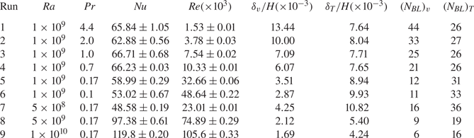
Table 1 lists a summary of the parameters used for simulations at different Rayleigh numbers and Prandtl numbers. In table 1, we also include the numerically calculated values of the local Nusselt number  $Nu$, the Reynolds number $Re$, the normalised viscous boundary-layer thickness $\delta _v/H$ and the normalised thermal boundary-layer thickness $\delta _T/H$. Here the local Nusselt number is defined as $Nu=-\partial _z T|_{z=0}H/\Delta T$ and the Reynolds number is defined as $Re=U_mH/\nu$. The definition of the viscous and thermal boundary-layer thicknesses, $\delta _v$ and $\delta _T$, are given in (4.4) and (4.18), respectively. For all the DNS runs, we use the same aspect ratio $\varGamma =0.2$ and the same total number of spectral elements, $N_{e}=96768$.
DNS runs at different Rayleigh numbers ( $Ra$) and Prandtl numbers ( $Pr$). The parameters used in the DNS runs include the number $(N_{BL})_v$ of grid points used to resolve the viscous boundary layer of dimensionless thickness $\delta _v/H$ and the number $(N_{BL})_T$ of grid points used to resolve the thermal boundary layer of dimensionless thickness $\delta _T/H$. Also included are the numerically calculated values of the local Nusselt number $Nu$, the Reynolds number $Re$, the normalised viscous boundary-layer thickness $\delta _v/H$, and the normalised thermal boundary-layer thickness $\delta _T/H$. For all the DNS runs, we used the same aspect ratio $\varGamma =0.2$, the same number of spectral elements across the circular cross-sectional area $(N_{e})_{x,z}=8064$, the same number of spectral elements along the thickness direction $(N_{e})_{y}=12$, and the same total number of spectral elements, $N_{e}=(N_{e})_{x,z}(N_{e})_{y}=96768$.
3. Comparison of the temperature and velocity fields between the low- and high- $Pr$ fluids

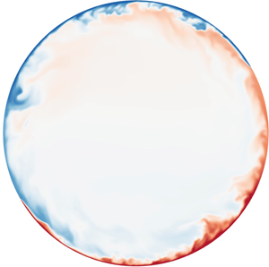
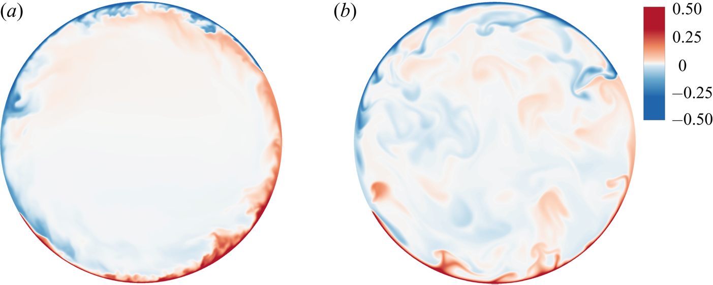
Figure 2 shows the contour plots of the instantaneous 2-D temperature field on the middle cross-section for two Prandtl numbers:  $Pr=0.17$ and $Pr=4.4$. It is found that warm rising plumes (in red) are generated from the bottom conducting plate and cold falling plumes (in blue) are generated from the top plate. These plumes drive the LSC. Because the low- $Pr$ fluid has a relatively larger thermal diffusivity, the thermal plumes in the low- $Pr$ fluid have a shorter lifetime. As a result, they have a lower chance to move into the bulk region and most of them are concentrated in the narrow region near the curved sidewall. On the other hand, the thermal plumes in the high- $Pr$ fluid have a longer lifetime and thus they have a higher chance to be found in the bulk region.
Contour plots of the instantaneous temperature field across the middle cross-section of the cell at (a)  $Pr=0.17$ and (b) $Pr=4.4$. The simulations are conducted at $Ra=1\times 10^9$ in a vertical thin disk with $\varGamma =0.2$. The colour code is shown with dark red for the highest dimensionless temperature 0.5 (bottom heating plate) and dark blue for the lowest dimensionless temperature $-$0.5 (top cooling plate). The data are shown in a linear scale ranging from $-$0.5 to 0.5.
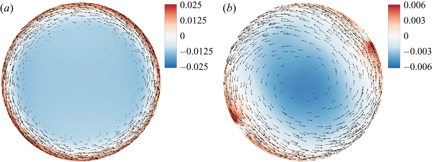
The spatial distribution of the thermal plumes has a profound influence on the velocity field. Figure 3 shows a comparison of the in-plane mean velocity field and corresponding mean pressure field across the middle cross-section of the cell between two Prandtl numbers: ( $a$)
$a$)  $Pr=0.17$ and ( $b$)
$b$)  $Pr=4.4$. It is seen that the mean flow field in the low- $Pr$ fluid is more coherent and has a mean flow concentrated mainly in the narrow region near the circular sidewall. The pressure contour in the bulk region shows a homogeneous circular shape, which fits nicely to the circular sidewall. This pressure field provides a long-range homogeneous shear flow along the conducting plates. Owing to the rotational symmetry of the LSC, the pressure gradient along the conducting plates is negligibly small. The thin disk cell thus offers a simple flow structure for the study of the intrinsic properties of the LSC and boundary layers at low $Pr$. The mean flow field in the high- $Pr$ fluid, however, has more spatial variations and spreads deep inside the bulk region. The pressure contour in the bulk region shows a slightly tilted elliptical shape, which is caused by the accumulation of rising warm plumes on the lower right region and falling cold plumes on the upper left region. On the other hand, the mean velocity and pressure fields in convection cells of other shapes, such as thin square cells and cylinders of aspect ratio unity, are very different from those shown in figure 3. Previous numerical studies (Xu Reference Xu2014; Chong et al. Reference Chong, Wagner, Kaczorowski, Shishkina and Xia2018) have revealed that the mean velocity field in thin square cells has a large tilted LSC in the bulk region, which coexists with two small rolls of opposite rotation located in two opposing corners of the cell. Similar corner flows were also observed experimentally by particle image velocimetry in cylindrical cells (Sun et al. Reference Sun, Xia and Tong2005). The interaction between the corner flow and LSC generates a complex structure near the conducting plates, which is different from the simple shear flow assumed by most boundary-layer theories. As shown in figure 3, no corner flow is observed in the thin disk cell.
Vector plots of the in-plane mean velocity field and contour plots of the mean pressure field across the middle cross-section of the cell at (a)  $Pr=0.17$ and (b) $Pr=4.4$. The simulations are conducted at $Ra=1\times 10^9$ in a vertical thin disk with $\varGamma =0.2$. The colour code is shown with dark red for the highest pressure and dark blue for the lowest pressure in unit of $\rho U_{f}^2$.
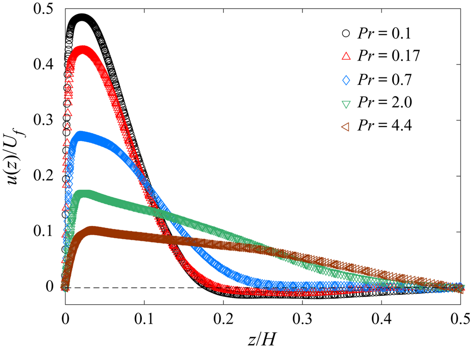
To describe the velocity field more quantitatively, we show, in figure 4, the normalised mean horizontal velocity profile  $u(z)/U_{f}$ as a function of the normalised vertical distance $z/H$ for five different values of $Pr$. At $Pr=4.4$, the bulk flow behaves like a rigid-body rotation with a zero mean velocity at the cell centre. The mean velocity increases linearly with the radial distance away from the cell centre. Similar single-roll structures of the LSC were also observed in the upright cylindrical cells of aspect ratio unity (Du & Tong Reference Du and Tong2000; Qiu & Tong Reference Qiu and Tong2001; Xi et al. Reference Xi, Lam and Xia2004; Sun et al. Reference Sun, Xia and Tong2005; Song & Tong Reference Song and Tong2010). As $Pr$ decreases, the effect of the fluid viscosity decreases and the rotation speed of the LSC increases. The faster rotation of the LSC gives the thermal plumes less time to penetrate into the bulk region. As a result, $u(z)/U_{f}$ moves to the region near the circular sidewall. At $Pr=0.17$, the obtained $u(z)/U_{f}$ behaves like a near-wall jet with a sharp velocity peak near the bottom plate. The strong near-wall flow, in turn, produces a large entrainment effect carrying the thermal plumes in the narrow near-wall region. The strong coupling between the LSC and thermal plumes is self-organised so that a continuous LSC is maintained even when the thermal plumes have a short lifetime. The shape of the near-wall jet remains approximately the same when $Pr$ is further reduced to 0.1. This result suggests that the flow has reached a new steady-state regime at low $Pr$.
$Pr$.
Normalised mean horizontal velocity profiles  $u(z)/U_{f}$ as a function of the normalised vertical distance $z/H$ away from the centre of the bottom conducting plate for five values of $Pr$: 0.1 (black circles), 0.17 (red up triangles), 0.7 (blue diamonds), 2.0 (green down triangles) and 4.4 (brown left triangles). The simulations are conducted at $Ra=1\times 10^9$ in a vertical thin disk with $\varGamma =0.2$.
In the following, we investigate the functional form of the normalised mean horizontal velocity profile  $\tilde {u}(z)\equiv u(z)/U_m$ and the normalised mean temperature profile $\theta (z) \equiv [T_{b}-T(z)]/\Delta _b$, where $T(z)$ is the actual mean temperature profile, $T_{b}$ is the bottom plate temperature and $\Delta _b$ is the temperature difference across the bottom thermal boundary layer. This study is carried out at a fixed $Pr=0.17$ and a fixed aspect ratio $\varGamma =0.2$. As mentioned previously, $Pr=0.17$ is chosen because the flow has reached a new steady-state regime at low $Pr$ and the DNS results can be obtained more efficiently and be used for comparison with future experiments using a gas mixture of H $_2$ and Xe (Bajaj et al. Reference Bajaj, Ahlers and Pesch2002).
4. Mean horizontal velocity and temperature profiles in the boundary-layer region
To find the functional form of the mean horizontal velocity and temperature profiles in the boundary-layer region, we consider a 2-D convective flow over a long horizontal heating plate with a constant horizontal mean velocity  $U_{m}$. Using the coordinate system shown in figure 1(a) and taking the Reynolds decomposition of the velocity field $\boldsymbol {u}(\boldsymbol {r},t)=\langle {\boldsymbol {u}}\rangle (\boldsymbol {r})+\boldsymbol {u}'(\boldsymbol {r},t)$ and temperature field $T(\boldsymbol {r},t)=\langle {T}\rangle (\boldsymbol {r})+T'(\boldsymbol {r},t)$, we obtain the viscous and thermal boundary-layer equations
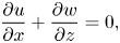 \begin{gather} \frac{\partial u}{\partial x}+\frac{\partial w}{\partial z}=0, \end{gather}
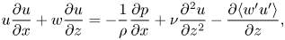 \begin{gather}u\frac{\partial u}{\partial x}+w\frac{\partial u}{\partial z}={-}\frac{1}{\rho}\frac{\partial p}{\partial x}+\nu\frac{\partial^2 u}{\partial z^2}-\frac{\partial\langle{w'u'}\rangle}{\partial z}, \end{gather}
 \begin{gather}u\frac{\partial T}{\partial x}+w\frac{\partial T}{\partial z}=\kappa\frac{\partial^2 T}{\partial z^2}-\frac{\partial\langle{w'T'}\rangle}{\partial z}, \end{gather}
where all the time-average notation  $\langle {\cdot }\rangle$ on the first-order terms are omitted for conciseness. These equations are obtained by applying the boundary-layer approximations $|{w}|\ll |{u}|$, $|\partial /\partial x|\ll |\partial /\partial z|$ and $|\partial ^2/\partial x^2|\ll |\partial ^2/\partial z^2|$, and a long time average to the dimensional form of (2.2) and (2.3). Based on the boundary-layer approximations and dimensional analysis, we find that the convection and diffusion terms in the vertical direction are much smaller than those in the horizontal direction, as shown in (4.2). As a result, only the pressure gradient and buoyancy terms remain in the viscous boundary-layer equation in the vertical direction, namely, $\rho ^{-1}\partial _zp=g\alpha (T-T_0)$ (Ching et al. Reference Ching, Leung, Zwirner and Shishkina2019). As shown in figure 3(a) and more quantitatively in figure 5(a), the pressure gradient term $\rho ^{-1}\partial _x p$ in (4.2) is negligibly small, so that the vertical pressure–buoyancy balance equation does not affect the above viscous and thermal boundary-layer equations explicitly. For low- $Pr$ RBC, we still expect the classical boundary-layer assumptions to be valid for both the viscous and thermal boundary layers. This is because the thicknesses of the two boundary layers are comparable at $Pr=0.17$, with the thickness ratio between the viscous and thermal boundary layers being $Pr^{1/2}\simeq 0.4$.
(a) Contributions of the mean convection term  $u\partial _x u+w\partial _z u$, molecular momentum diffusion components $-\nu \partial _x^2 u$ and $-\nu \partial _z^2 u$, Reynolds stress gradient components $\partial _x \langle u'u'\rangle$ and $\partial _z \langle w'u'\rangle$, and pressure gradient $1/\rho \partial _x p$, as a function of the normalised vertical distance $z/\delta _{v}$. The unit of the terms is $U_{f}^2/H$. The two solid lines show the calculated terms of the velocity equation using the analytical solution $\tilde {u}(\xi )$ in (4.14) with $a=1.19$. (b) Contributions of the mean convection term $u\partial _x T+w\partial _z T$, molecular thermal diffusion components $-\kappa \partial _x^2 T$ and $-\kappa \partial _z^2 T$, and turbulent heat flux gradient components $\partial _x \langle u'T'\rangle$ and $\partial _z \langle w'T'\rangle$, as a function of $z/\delta _{v}$. The unit of the terms is $U_{f}\Delta T/H$. The DNS data used for the calculations shown in (a) and (b) are obtained at $Pr=0.17$ and $Ra=1\times 10^9$ in a vertical thin disk with $\varGamma =0.2$.

With the DNS data, we numerically calculate the contributions of each term in the mean velocity equation and the mean temperature equation. Figures 5(a) and 5(b) show, respectively, the terms of the velocity and temperature equations as a function of the normalised vertical distance  $z/\delta _{v}$ away from the bottom conducting plate. Here the viscous boundary-layer thickness $\delta _{v}$ is defined as a vertical distance, at which the tangent of the mean velocity profile at the bottom plate ( $z=0$) intersects the maximum velocity $U_{{m}}$, namely
 \begin{equation} \delta_{v}=U_{m}\left|\frac{\partial u}{\partial z}\right|^{{-}1}_{z=0}. \end{equation}
It can be seen from figure 5(a) that the boundary-layer approximations hold for the mean velocity equations in the near-wall region. We verify numerically that the horizontal pressure gradient  $\rho ^{-1}\partial _xp$ is negligible at low $Pr$ so that the viscous boundary-layer equation (4.2) is decoupled from the thermal boundary-layer equation (4.3) (Ching et al. Reference Ching, Leung, Zwirner and Shishkina2019). In addition, we find numerically that the mean convection term, $u\partial _xu+w\partial _zu$, in (4.2) is negligibly small for this low- $Pr$ RBC system. As a result, only two dominant terms remain in the mean velocity equation (4.2), namely, the molecular momentum diffusion $\nu \partial _z^2 u$ and turbulent momentum diffusion $\partial _z\langle {w'u'}\rangle$, which balance each other in the near-wall region,
 \begin{equation} \nu\frac{\partial^2 u}{\partial z^2}=\frac{\partial\langle{w'u'}\rangle}{\partial z}. \end{equation}
 Similarly, the mean temperature equation (4.3) also has two dominant terms, namely, the molecular thermal diffusion  $\kappa \partial _z^2T$ and turbulent thermal diffusion $\partial _z\langle {w'T'}\rangle$. There is a small contribution from the mean convection term, $u\partial _xT+w\partial _zT$, for $Ra=5\times 10^8$. From the DNS results, we find the contribution of the mean convection decreases with increasing $Ra$. As shown in figure 5(b), the mean convection can be approximately ignored for $Ra=1\times 10^9$. Therefore, in the $Ra$ range $1\times 10^9\leq Ra \leq 1\times 10^{10}$, we have
 \begin{equation} \kappa\frac{\partial^2 T}{\partial z^2}\simeq\frac{\partial\langle{w'T'}\rangle}{\partial z}. \end{equation}
4.1. Mean horizontal velocity profile in the boundary-layer region
With the turbulent viscosity  $\nu _t(z)$ defined as
 \begin{equation} \langle{w'u'}\rangle={-}\nu_t(z)\frac{\mathrm{d} u}{\mathrm{d} z}, \end{equation}
equation (4.5) becomes an ordinary differential equation
 \begin{equation} \left(1+\frac{\nu_t}{\nu}\right)\frac{\mathrm{d}^2 u}{\mathrm{d} z^2}+\frac{\mathrm{d}}{\mathrm{d} z}\left(1+\frac{\nu_t}{\nu}\right)\frac{\mathrm{d} u}{\mathrm{d} z}=0. \end{equation}
Integrating both sides and applying the definition (4.4) as the boundary condition, we obtain
 \begin{equation} \frac{\mathrm{d} u}{\mathrm{d} z}=\frac{U_m/\delta_v}{1+\nu_t/\nu}. \end{equation}
The formal solution of (4.9) is given by
 \begin{equation} \tilde{u}(\xi)=\int_0^{\xi}\frac{1}{1+\nu_t(s)/\nu}\,\mathrm{d} s, \end{equation}
where  $\tilde {u}=u/U_{m}$ and $\xi =z/\delta _{v}$.
With the no-slip boundary condition at the bottom conducting plate, we find the Reynolds stress  $\langle {w'u'}\rangle$ and its derivatives satisfy the following boundary conditions at $z=0$,
 \begin{equation} \langle{w'u'}\rangle=\partial_z\langle{w'u'}\rangle=\partial_z^2\langle{w'u'}\rangle=0. \end{equation}
From the definition of  $\nu _t$ in (4.7) and the linear velocity profile at the wall, i.e. $\mathrm {d} u/\mathrm {d} z\propto z^0$, we obtain the boundary conditions for $\nu _t$ at $\xi =0$,
 \begin{equation} \nu_t(0)=(\nu_t)_\xi(0)=(\nu_t)_{\xi\xi}(0)=0. \end{equation}
Therefore, the leading order of  $\nu _t$ has the form
 \begin{equation} \nu_t/\nu\simeq a^3\xi^3, \end{equation}
where  $a$ is a constant. A similar boundary condition was also obtained for $\kappa _t/\kappa$ in the thermal boundary-layer equation (Shishkina et al. Reference Shishkina, Horn, Wagner and Ching2015). Substituting (4.13) into (4.10), we obtain the analytical form of the normalised horizontal velocity profile
 \begin{equation} \tilde{u}(\xi)=\frac{1}{6a}\ln\frac{(1+a\xi)^3}{1+(a\xi)^3}+\frac{\sqrt{3}}{3a} \arctan\frac{2a\xi-1}{\sqrt{3}}+\frac{\sqrt{3}\pi}{18a}. \end{equation}
 Figure 6(a) shows the normalised turbulent viscosity  $\nu _t/\nu$ as a function of the normalised vertical distance $z/\delta _v$. Using (4.7), we numerically calculate $\nu _t=-\langle {w'u'}\rangle /(\mathrm {d} u/\mathrm {d} z)$. For all three values of $Ra$, the obtained $\nu _t/\nu$ is well described by (4.13) with $a=1.19$ (green dashed line) for small values of $z$ up to $z/\delta _v\lesssim 2$. Deviations from the green dashed line are observed when $z/\delta _{v} \gtrsim 2$. These deviations exhibit an interesting dependence on $Ra$, with the obtained $\nu _t/\nu$ at $Ra=1\times 10^9$ as an exceptional case, which has a wider power-law range up to $z/\delta _v\simeq 6$. With the obtained $\nu _t/\nu$ in figure 6(a), we numerically compute the solution of (4.10), as shown by the three solid lines in figure 6(b) for the three different values of $Ra$. It is seen that the agreement between the numerical solutions of (4.10) and the DNS data (open symbols) improves significantly with increasing $Ra$. A small deviation between the green solid line and black circles is observed at larger values of $z/\delta _v$ for $Ra=5\times 10^8$. This is caused by the fact that for small values of $Ra$, a small contribution from the mean convection term becomes noticeable, which affects the accuracy of (4.5). Because the obtained $\nu _t/\nu$ at $Ra=1\times 10^9$ is well described by (4.13) with $a=1.19$ over a wider range of $z/\delta _v$, the corresponding velocity profile $u/U_{m}$ as a function of $z/\delta _{v}$ (red triangles in figure 6b) is equally well described by (4.14) with the same fitting parameter $a=1.19$. By assuming (4.13) holds for distances far enough from the wall, one may use the asymptotic boundary condition, $\tilde {u}(\infty )=1$, to determine the value of $a=2\sqrt {3}\pi /9\simeq 1.2$. The fitted value of $a=1.19$ is very close to this limiting value. Figure 6 thus confirms that the viscous boundary-layer model discussed earlier captures the essential physics.
(a) Log–log plots of the normalised turbulent viscosity  $\nu _t/\nu$ as a function of $z/\delta _{v}$ for $Ra=5\times 10^8$ (black circles), $1\times 10^{9}$ (red triangles) and $1\times 10^{10}$ (blue diamonds). The green dashed line shows a fit to (4.13) with $a=1.19$. The vertical dashed line indicates the edge of the viscous boundary layer with $z/\delta _{v}=1$. (b) Normalised mean horizontal velocity profile $u/U_{m}$ as a function of $z/\delta _{v}$ for $Ra=5\times 10^8$ (black circles), $1\times 10^{9}$ (red triangles) and $1\times 10^{10}$ (blue diamonds). The green, blue and brown solid lines show, respectively, the numerical solutions of (4.10) using the numerically calculated $\nu _t/\nu$ shown in (a) for $Ra=5\times 10^8$, $1\times 10^{9}$ and $1\times 10^{10}$. The DNS data used for the calculations shown in (a) and (b) are obtained at $Pr=0.17$ in a vertical thin disk with $\varGamma =0.2$.

4.2. Mean temperature profile in the boundary-layer region
Using the turbulent thermal diffusivity  $\kappa _t(z)$ defined as
 \begin{equation} \langle{w'T'}\rangle={-}\kappa_t(z)\frac{\mathrm{d} T}{\mathrm{d} z}, \end{equation}
equation (4.6) becomes an ordinary differential equation
 \begin{equation} \left(1+\frac{\kappa_t}{\kappa}\right)\frac{\mathrm{d}^2 T}{\mathrm{d} z^2}+\frac{\mathrm{d}}{\mathrm{d} z}\left(1+\frac{\kappa_t}{\kappa}\right)\frac{\mathrm{d} T}{\mathrm{d} z}=0. \end{equation}
Integrating both sides and applying the relation at the boundary,
 \begin{equation} \delta_{T}=\Delta_b\left|\frac{\partial T}{\partial z}\right|^{{-}1}_{z=0}, \end{equation}
which defines the thermal boundary-layer thickness  $\delta _{T}$, we obtain
 \begin{equation} \frac{\mathrm{d} T}{\mathrm{d} z}={-}\frac{\Delta_b/\delta_T}{1+\kappa_t/\kappa}. \end{equation}
The formal solution of (4.18) is given by
 \begin{equation} \theta(\xi)=\frac{\delta_{v}}{\delta_T}\int_0^{\xi}\frac{1}{1+\kappa_t(s)/\kappa}\mathrm{d} s, \end{equation}
where  $\theta (z)=[T_{b}-T(z)]/\Delta _b$ and $\xi =z/\delta _v$.
For high- $Pr$ RBC, the thermal boundary layer is nested within the viscous boundary layer, so that $\kappa _t(z)$ obeys a cubic power law similar to (4.13) across the entire thermal boundary layer. In this case, the mean temperature profile $\theta (\xi )$ takes the same functional form as shown in (4.14). This was shown previously by Shishkina et al. (Reference Shishkina, Horn, Wagner and Ching2015). For low- $Pr$ RBC, however, the thermal boundary layer is thicker than the viscous boundary layer, so that the LSC may produce a strong shear on the outer portion of the thermal boundary layer, as illustrated in figure 7(a). The numerically calculated $\kappa _t(z)$ for $Pr=0.17$ is found to obey the cubic power law in (4.13) only up to $z/\delta _{v}\simeq 1$. This is shown in figure 7(b). Outside the viscous boundary layer (but still within the thermal boundary layer), the obtained $\kappa _t(z)$ goes as $z^{2.2}$ with the power-law exponent being smaller than 3. In this case, no analytical solution of (4.19) is available and one needs to numerically integrate (4.19). The situation is somewhat similar to a boundary layer near a partial-slip wall, as illustrated in figure 7(a). Owing to the large streamwise velocity at the edge of the viscous boundary layer, $\partial _z^2\langle {w'T'}\rangle$ is no longer guaranteed to be zero, so that the leading order of $\kappa _t$ is reduced from $z^3$ to $z^2$ (authors' unpublished observations).
(a) Sketch of the viscous boundary layer and thermal boundary layer at low  $Pr$, in which the viscous boundary layer is nested within the thermal boundary layer. (b) Log–log plots of the normalised turbulent diffusivity $\kappa _t/\kappa$ as a function of $z/\delta _{v}$ for $Ra=5\times 10^8$ (black circles), $1\times 10^{9}$ (red triangles) and $1\times 10^{10}$ (blue diamonds). The green dashed line shows a cubic power law $\kappa _t/\kappa =0.45(z/\delta _{v})^3$. The DNS data used for the calculations are obtained at $Pr=0.17$ in a vertical thin disk with $\varGamma =0.2$.
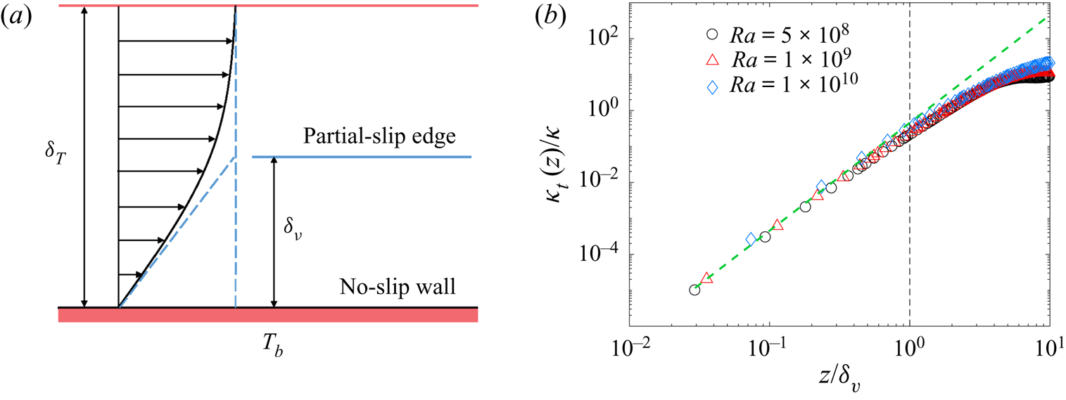
With the obtained  $\kappa _t/\kappa$ in figure 7(b), we numerically compute the solution of (4.19), as shown by the three solid lines in figure 8 for the three different values of $Ra$. It is seen that the agreement between the numerical solutions of (4.19) and the DNS data (open symbols) improves significantly with increasing $Ra$. Small deviations are observed at larger values of $z/\delta _v$ for the two lower values of $Ra$. This is caused by the fact that for small values of $Ra$, a small contribution from the mean convection term becomes noticeable (see figure 5b), which affects the accuracy of (4.6). The good agreement between the calculated solution of (4.19) and the DNS result at $Ra=1\times 10^{10}$ further confirms that the thermal boundary-layer model discussed previously captures the essential physics.
Normalised mean temperature profile  $\theta (z)$ as a function of $z/\delta _{v}$ for $Ra=5\times 10^8$ (black circles), $1\times 10^{9}$ (red triangles) and $1\times 10^{10}$ (blue diamonds). The green, blue and brown solid lines show, respectively, the numerical solutions of (4.19) using the numerically calculated $\kappa _t/\kappa$ shown in figure 7(b) for $Ra=5\times 10^8$, $1\times 10^{9}$ and $1\times 10^{10}$. The DNS data used for the calculations are obtained at $Pr=0.17$ in a vertical thin disk with $\varGamma =0.2$.
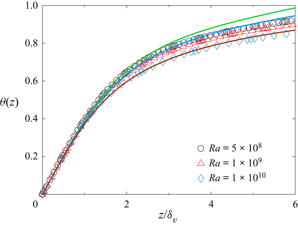
5. Mean horizontal velocity profile in the bulk region
Figure 9(a) shows the terms of the velocity equation as a function of the normalised vertical distance  $z/H$. Compared with those terms in the boundary-layer region, all of the terms are small in the bulk region. Among them, the mean convection and the vertical Reynolds stress gradient decay with $z/H$ much slower than the other terms. By balancing the mean convection with the vertical Reynolds stress gradient, we have
 \begin{equation} u\frac{\partial u}{\partial x}+w\frac{\partial u}{\partial z}={-}\frac{\partial\langle{w'u'}\rangle}{\partial z}. \end{equation}
As shown in figure 9(b), the turbulent viscosity  $\nu _t(x,z)$ in the bulk region is approximately independent of $z$ and, therefore, we have
 \begin{equation} \langle{w'u'}\rangle={-}\nu_t(x)\frac{\partial u}{\partial z}. \end{equation}
Substituting (5.2) into (5.1), we obtain
 \begin{equation} {u}\frac{\partial{u}}{\partial x}+{w}\frac{\partial{u}}{\partial z}=\nu_t(x)\frac{\partial^2{u}}{\partial z^2}. \end{equation}
(a) Contributions of mean convection  $u\partial _x u+w\partial _z u$ (black circles), vertical molecular momentum diffusion $-\nu \partial _z^2u$ (blue diamonds) and vertical Reynolds stress gradient $\partial _z \langle w'u'\rangle$ (brown triangles) as a function of the normalised vertical distance $z/H$ for $Ra=1\times 10^9$. The unit of the terms is $U_{f}^2/H$. (b) Normalised turbulent viscosity $\nu _t(z)/(U_{f}H)$ as a function of $z/H$ for three values of $Ra$:
$Ra$:  $5\times 10^8$ (black circles), $1\times 10^9$ (red triangles) and $1\times 10^{10}$ (blue diamonds). The DNS data used for the calculations shown in (a) and (b) are obtained at $Pr=0.17$ in a vertical thin disk with $\varGamma =0.2$.
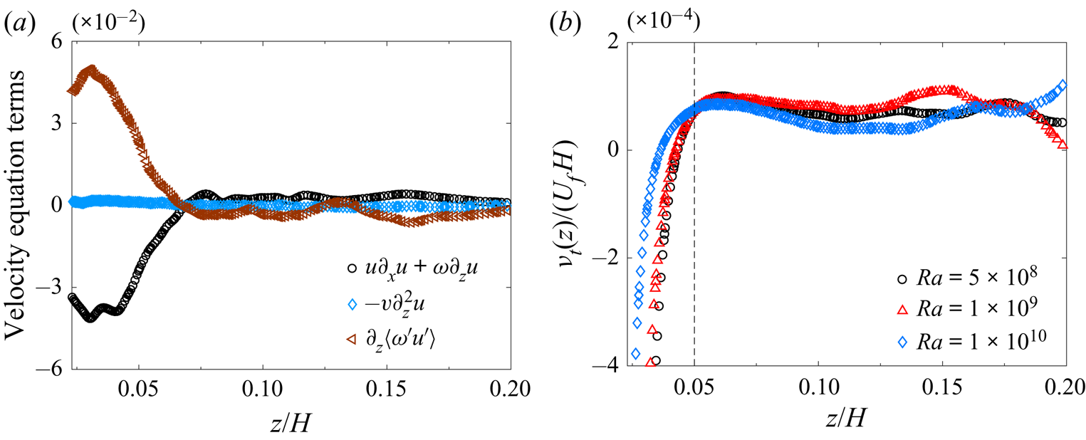
Equation (5.3) admits a self-similarity solution for a free turbulent jet (Pope Reference Pope2000). By assuming the large-scale flow in the bulk region is a half turbulent jet, we find
 \begin{equation} \tilde{u}=1-\tanh^2\left(\frac{z-z_0}{\eta}\right), \end{equation}
where  $\tilde {u}=u/U_m$, $z_0$ is the starting position of the half-jet, and $\eta$ represents the jet width,
 \begin{equation} \eta=2\sqrt{\frac{\nu_t x}{U_{m}}}. \end{equation}
 Figure 10(a) shows the normalised mean horizontal velocity profile  $u(z)/U_{f}$ as a function of $z/H$. It is seen that all of the numerically calculated $u(z)/U_{f}$ for different values of $Ra$ collapse approximately on to a single master curve. This suggests that the obtained $u(z)/U_{f}$ in the bulk region is approximately a scaling function of $z/H$, which is invariant with $Ra$. From figures 9(b) and 10(a), we find $\nu _t\simeq 1.0\times 10^{-4}U_fH$ and $U_m\simeq 0.42U_f$. By assuming the streamwise length $x$ scales with the circumference $\pi H$ of the circular disk, i.e. $x\simeq \pi H$, we obtain the jet width $\eta \simeq 0.055H$ from (5.5). This result thus explains why the numerically calculated $u(z)/U_{f}$ in the bulk region is a scaling function of $z/H$. In addition, figure 10(b) shows that the obtained $u(z)/U_{f}$ is adequately described by (5.4) and the fitted values of $\eta$ is $0.08H$, which also agrees with the estimated value of $\eta \simeq 0.055H$ by (5.5). The good agreement between the DNS results and the analytical solution confirms that the turbulent jet model discussed above captures the essential physics. We also compute $u(z)/U_{f}$ in the $\varGamma =0.1$ disk cell and the resulting $u(z)/U_{f}$ exhibits a similar shape of near-wall jet, as shown in figure 10(a). However, both the maximal value of the jet and its width show a weak $Ra$-dependence. Because the jet width in the $\varGamma =0.1$ cell is comparable to the disk thickness, we suspect that this weak $Ra$-dependence is caused by the confinement effect of the thin disk. Indeed, when the disk thickness is increased to $\varGamma =0.2$, the obtained $u(z)/U_{f}$ is found to have an approximate universal form, as shown in figure 10(a), which does not change significantly with $Ra$.
$Ra$.
(a) Normalised mean horizontal velocity profiles  $u(z)/U_{f}$ as a function of the normalised vertical distance $z/H$ for three different values of $Ra$:
$Ra$:  $5\times 10^8$ (black circles), $1\times 10^9$ (red triangles) and $1\times 10^{10}$ (blue diamonds). (b) Replot of the mean horizontal velocity profiles $u/U_{m}$ normalised by its maximum value $U_{m}$ as a function of $z/H$ for $Ra=5\times 10^8$ (black circles), $1\times 10^9$ (red triangles) and $1\times 10^{10}$ (blue diamonds). For clarity, the origin of the red and blue curves is shift to the right by $0.1$ and $0.2$ normalised distances, respectively. The green, blue and brown solid lines show the same plot of (5.4) with $\eta =0.08H$ and $z_0=0.02H$. The DNS data used for the calculations shown in (a) and (b) are obtained at $Pr=0.17$ in a vertical thin disk with $\varGamma =0.2$.

6. Summary
We have carried out a systematic numerical study of the mean velocity and temperature profiles in turbulent Rayleigh–Bénard convection at low Prandtl numbers. The DNS runs were conducted in a vertical thin disk with the Prandtl number ( $Pr$) varied in the range $0.17\leq Pr\leq 4.4$ and the Rayleigh number ( $Ra$) varied between $5\times 10^8$ and $1\times 10^{10}$. For a fixed value of $Ra = 5\times 10^9$ and with varying values of $Pr$ from 4.4 to 0.17, we find a sharp change of flow patterns for the LSC. For high- $Pr$ RBC, the lifetime of thermal plumes is longer so that they have a better chance to enter the bulk region and drive the flow globally. As a result, the LSC in high- $Pr$ RBC rotates like a rigid body. For low- $Pr$ RBC, however, the thermal plumes have a shorter lifetime so that they have less chance of surviving in the bulk region. Consequently, the thermal plumes are concentrated in the near-wall region and the LSC in low- $Pr$ RBC behaves like a near-wall turbulent jet.
For low- $Pr$ RBC, the viscous boundary layer is nested inside the thermal boundary layer. Thus, the strong shearing effect by the viscous boundary layer causes the thermal boundary layer to be separated into two sub-layers. This effect makes the thermal boundary layer at low $Pr$ more complicated than that at high $Pr$. We numerically examine the mean velocity and temperature equations in the boundary-layer region and find that both the mean horizontal velocity profile $u(z)$ and temperature profile $T(z)$ can be determined by a balance equation between the molecular diffusion and turbulent diffusion. Furthermore, the no-slip boundary condition at the bottom conducting wall dictates that both the turbulent viscosity $\nu _t(z)$ and turbulent thermal diffusivity $\kappa _t(z)$ as a function of distance $z$ away from the bottom conducting wall obey a cubic power law ( $\sim z^3$) for small values of $z$ within the viscous boundary layer. In this case, both $u(z)$ and $T(z)$ can be solved analytically and the solutions agree well with the DNS data. Owing to the large streamwise velocity at the edge of the viscous boundary layer, the leading order of the obtained $\kappa _t(z)$ at larger values of $z$ outside the viscous boundary layer (but still within the thermal boundary layer) is reduced from $z^3$ to $z^2$. In this case, the mean temperature profile $T(z)$ can be solved numerically using the calculated $\kappa _t(z)$.
For a fixed value of  $Pr=0.17$ and with varying $Ra$ in the range $5\times 10^8\leq Ra \leq 1\times 10^{10}$, we find that the mean horizontal velocity profile $u(z)$ can be determined by an equation with the mean convection balanced by turbulent diffusion with a $z$-independent turbulent viscosity $\nu _t$. This balance equation admits a self-similarity jet solution, which fits the DNS data well. The width $\eta$ of the near-wall jet is determined by the diffusion equation $\eta ^2=4\nu _t\tau$, where $\tau \simeq \pi H/U_m$ is the turnover time of the LSC with $\pi H$ being the circumference of the circular disk and $U_m$ is the maximum velocity of the LSC. Our DNS data also reveal that the azimuthal velocity profiles at different polar angles $\theta$ have a similar near-wall jet shape, as shown in figure 10. However, the peak velocity $U_m$ has a weak angular dependence. We believe that this is caused by the angular dependence of the buoyancy term, $g\sin \theta$, where $g$ is the gravitational acceleration. Owing to this buoyancy term, the momentum equation is coupled to the thermal equation, which makes the problem difficult to solve mathematically. Here we choose the vertical $z$-direction with $\theta =0$, so that the two equations are decoupled. In this case, we find a simple mathematical solution to describe the vertical profile of the mean horizontal velocity $u(z)$, which captures the essential feature of the LSC in low- $Pr$ RBC.
Our work thus provides a full characterisation of the mean velocity and temperature profiles in low- $Pr$ RBC. This characterisation allows us to further understand the intricate interplay between the LSC, plume emission and boundary-layer dynamics, and pinpoint the physical mechanism for the emergence of a pronounced LSC in low- $Pr$ RBC. This study lays down a foundation for further study of the effects of cell shape and confinement by cell end walls, as reported by Chong et al. (Reference Chong, Wagner, Kaczorowski, Shishkina and Xia2018) for a different cell geometry.
Acknowledgements
We would like to thank Prof. Emily S. C. Ching and Dr. G. Y. Cao for useful discussions. This work was supported in part by the Hong Kong Research Grants Council under grant nos. 16301719 (P.T.), N_HKUST604/19 (P.T.) and 16305819 (X.W.) and by the National Natural Science Foundation of China under grant nos. 11772111 (X.H.), 91952101 (X.H.), 11702128 (S.H.), 11961160719 (S.H.) and 91752201 (S.H.). J.S. acknowledges support by the Deutsche Forschungsgemeinschaft within the Priority Programme DFG-SPP 1881 on Turbulent Superstructures.
Declaration of Interests
The authors report no conflict of interest.


 Open access