





1. Introduction
Understanding the interplay between complex surface geometry and non-Newtonian effects in shear flows is crucial across a wide range of applications, such as in the petroleum industry (Santos, Bannwart & Loh Reference Santos, Bannwart and Loh2014), food processing engineering (Steffe Reference Steffe1996) and physiology (Beris et al. Reference Beris, Horner, Jariwala, Armstrong and Wagner2021). Nevertheless, investigations of this coupling are comparatively rare. A recent example is the study of Kada et al. (Reference Kada, Pasha, Asghar, Khan, Aris and Shaikh2023), which investigated the laminar flow of shear-thinning fluid over walls coated with cilia in a two-dimensional channel. Only very recently, Narayanan et al. (Reference Narayanan, Singh, Nauer, Belt, Palermo and Lakehal2024) and Anbarlooei et al. (Reference Anbarlooei, Cruz, Celis, Macedo and Thompson2025) performed direct numerical simulations of generalised Newtonian fluids (GNFs) shear flow over a rough wall. In fluid mechanics, stability analysis is essential for understanding the transition to turbulence. However, surprisingly, no systematic study accounting for both geometrical and rheological effects appears to exist, based on our survey of different fluids and geometries.
A moderate amount of research has been conducted relating to the effect of sinusoidal wall undulation, the simplest non-trivial wall shape, on stability of Newtonian shear flows. Our interest concerns flows within axisymmetric corrugated pipes, which for Newtonian fluids have been investigated experimentally by Deiber & Schowalter (Reference Deiber and Schowalter1979), Nishimura et al. (Reference Nishimura, Ohori and Kawamura1984, Reference Nishimura, Bian, Matsumoto and Kunitsugu2003) and numerically by Saha et al. (Reference Saha, Klewicki, Ooi and Blackburn2015). With regards to stability, the numerical study most relevant to our work is that of Loh & Blackburn (Reference Loh and Blackburn2011), which investigated three-dimensional perturbations to laminar axisymmetric base flows. Using a corrugation wavelength comparable to the mean radius, perturbations with an azimuthal wavenumber $m=3$
were found to be unstable over a broad range of Reynolds numbers. Interestingly, this instability was found to be more dangerous than the axisymmetric perturbations previously identified by Lahbabi & Chang (Reference Lahbabi and Chang1986) and Cotrell, McFadden & Alder (Reference Cotrell, McFadden and Alder2008). In the studies of Cotrell et al. (Reference Cotrell, McFadden and Alder2008) and Loh & Blackburn (Reference Loh and Blackburn2011), the corrugation wavelength was fixed and commonly normalised to unity, such that the wall modulation could be written in a
$m=3$
were found to be unstable over a broad range of Reynolds numbers. Interestingly, this instability was found to be more dangerous than the axisymmetric perturbations previously identified by Lahbabi & Chang (Reference Lahbabi and Chang1986) and Cotrell, McFadden & Alder (Reference Cotrell, McFadden and Alder2008). In the studies of Cotrell et al. (Reference Cotrell, McFadden and Alder2008) and Loh & Blackburn (Reference Loh and Blackburn2011), the corrugation wavelength was fixed and commonly normalised to unity, such that the wall modulation could be written in a $2\pi$
-periodic form. This choice reflects a convenient normalisation and the imposition of axial periodicity required for Floquet or global-mode analyses, rather than a demonstration that this length scale is optimal.
$2\pi$
-periodic form. This choice reflects a convenient normalisation and the imposition of axial periodicity required for Floquet or global-mode analyses, rather than a demonstration that this length scale is optimal.
Channel flows with sinusoidally wavy walls have computationally simpler geometry and have been studied more extensively than corrugated pipe flows. The aforementioned axisymmetric instability in corrugated pipes arises from a mechanism similar to that identified in wavy two-dimensional channel flows (Cho, Kim & Shin Reference Cho, Kim and Shin1998; Selvarajan, Tulapurkara & Ram Reference Selvarajan, Tulapurkara and Ram1999; Floryan Reference Floryan2003; Blancher, Creff & Quéré Reference Blancher, Creff and Quéré2004; Floryan & Floryan Reference Floryan and Floryan2009). It is also worth noting that Haward et al. (Reference Haward, Page, Zaki and Shen2018) studied viscoelastic fluids to examine how the laminar state is modified by sinusoidal wall undulations. However, the instability identified by Loh & Blackburn (Reference Loh and Blackburn2011) is related to the ‘vortex instability’ found in channel flow by Floryan (Reference Floryan2003); see Floryan (Reference Floryan2005) also. We shall see that at high Reynolds numbers, this type of instability manifests more prominently in streaks than in vortices; for this reason, we refer to it as a streaky instability.
Hall (Reference Hall2020) showed that large-Reynolds-number-matched asymptotic expansion analysis can successfully explain the numerical results of Floryan (Reference Floryan2003, Reference Floryan2015). Shortly thereafter, the same type of asymptotic analysis was applied to pipe flow by Hall & Ozcakir (Reference Hall and Ozcakir2021). However, since the results of Loh & Blackburn (Reference Loh and Blackburn2011) did not extend to sufficiently high Reynolds numbers, it is not clear how reliable is the asymptotic approximation. Moreover, even for channel flows, the accuracy of the asymptotic predictions is only mediocre, raising the question of whether any improvement is possible. Addressing these issues is part of the objectives of the present study.
The primary aim of this paper is to generalise the stability analyses of Loh & Blackburn (Reference Loh and Blackburn2011) and Hall & Ozcakir (Reference Hall and Ozcakir2021) to flows of shear-thinning fluids. We employ the Carreau–Yasuda model, which belongs to the class of GNFs. This type of non-Newtonian model accounts for variable viscosity dependent only on local shear rate, excluding viscoelastic effects, but is a valid rheological model for many fluids (Chhabra & Richardson Reference Chhabra and Richardson2008). Owing to its simplicity, the GNF model is widely used in numerical computations; for example, Kada et al. (Reference Kada, Pasha, Asghar, Khan, Aris and Shaikh2023) and Anbarlooei et al. (Reference Anbarlooei, Cruz, Celis, Macedo and Thompson2025) used the Carreau–Yasuda model, while Narayanan et al. (Reference Narayanan, Singh, Nauer, Belt, Palermo and Lakehal2024) adopted the Herschel–Bulkley model. Both models are improved versions of the power-law model and contain the power-law index $n$
as a parameter. Numerical computations of strongly shear-thinning fluids (small
$n$
as a parameter. Numerical computations of strongly shear-thinning fluids (small $n$
) are particularly challenging, unless the Reynolds number is very low (see the comments of Plaut, Roland & Nouar Reference Plaut, Roland and Nouar2017; Anbarlooei et al. Reference Anbarlooei, Cruz, Celis, Macedo and Thompson2025, for example).
$n$
) are particularly challenging, unless the Reynolds number is very low (see the comments of Plaut, Roland & Nouar Reference Plaut, Roland and Nouar2017; Anbarlooei et al. Reference Anbarlooei, Cruz, Celis, Macedo and Thompson2025, for example).
The asymptotic analysis of Hall & Ozcakir (Reference Hall and Ozcakir2021) builds on the vortex-wave-interaction theory, originally developed to describe nonlinear coherent structures in smooth-wall shear flows (Hall & Smith Reference Hall and Smith1991). Subsequent studies (Hall & Sherwin Reference Hall and Sherwin2010; Blackburn, Hall & Sherwin Reference Blackburn, Hall and Sherwin2013; Deguchi & Hall Reference Deguchi and Hall2014, Reference Deguchi and Hall2016) have established that the asymptotic theory essentially captures the self-sustaining process (Hamilton, Kim & Waleffe Reference Hamilton, Kim and Waleffe1995; Waleffe Reference Waleffe1997), which describes the cyclic interaction of roll-streak-wave components in coherent structures. Numerical computations by Arosemena et al. (Reference Arosemena, Andersson, Andersson and Solsvik2021) using the Carreau–Yasuda model showed that the self-sustaining process is strongly affected by shear-thinning effects. Therefore, we also expect non-Newtonian effects to largely alter the streaky instability.
The paper is structured as follows. In the next section, we formulate the problem and introduce the three methods we use for stability analysis: high-order direct numerical simulation (DNS) (Blackburn et al. Reference Blackburn, Lee, Albrecht and Singh2019, Reference Blackburn, Rudman and Singh2025), high-Reynolds-number asymptotic analysis and an asymptotic-preserving reduction (APR). The third method is analogous to those used by Blackburn et al. (Reference Blackburn, Hall and Sherwin2013), Deguchi & Hall (Reference Deguchi and Hall2014) and Deguchi & Hall (Reference Deguchi and Hall2016) where the leading order terms and selected higher order contributions are retained to obtain a reduced form of the governing equations. The details of the reduction are explained in § 3. Section 4 then shows how to numerically solve the APR system and how the asymptotic analysis leads to an analytical neutral curve. In § 5, we compare the numerical results obtained using the three methods for moderately shear-thinning fluids and proceed with a parameter study of the neutral curve. We primarily explore general parameter regimes that advance the theoretical understanding of how wall undulations and shear-thinning affect streaky instabilities. We also perform analyses using fluid properties measured in experiments, although our aim is not to reproduce the experimental results. Finally, in § 6, we present our conclusions.
2. Formulation of the problem
Consider a shear-thinning fluid flowing through a pipe in cylindrical coordinates $(r^*,\theta ,z^*)$
. The pipe wall is defined by
$(r^*,\theta ,z^*)$
. The pipe wall is defined by $r^*=R^*(1+2\epsilon \cos (2\pi z^*/L^*))$
, where
$r^*=R^*(1+2\epsilon \cos (2\pi z^*/L^*))$
, where $2\epsilon$
denotes the relative amplitude of the wall undulation with respect to the mean pipe radius
$2\epsilon$
denotes the relative amplitude of the wall undulation with respect to the mean pipe radius $R^*$
. The factor of two on
$R^*$
. The factor of two on $\epsilon$
is introduced for convenience in the analysis of § 3. The wall shape has periodicity in the axial direction with the period
$\epsilon$
is introduced for convenience in the analysis of § 3. The wall shape has periodicity in the axial direction with the period $L^*$
. In a GNF model, the deviation from Newtonian behaviour arises solely through the dynamic viscosity
$L^*$
. In a GNF model, the deviation from Newtonian behaviour arises solely through the dynamic viscosity $\mu ^*$
in the Navier–Stokes equations. In general,
$\mu ^*$
in the Navier–Stokes equations. In general, $\mu ^*$
is a nonlinear function of the shear rate and its representative value at zero shear rate is denoted by
$\mu ^*$
is a nonlinear function of the shear rate and its representative value at zero shear rate is denoted by $\mu ^*_0$
.
$\mu ^*_0$
.
Throughout the paper, we use the length scale $R^*$
, velocity scale
$R^*$
, velocity scale $U_c^*$
and pressure scale
$U_c^*$
and pressure scale $\rho ^* U_c^{*2}$
, where
$\rho ^* U_c^{*2}$
, where $ \rho ^*$
is the fluid density and
$ \rho ^*$
is the fluid density and $U_c^*$
is the centreline velocity of the laminar base flow. Introducing the Reynolds number
$U_c^*$
is the centreline velocity of the laminar base flow. Introducing the Reynolds number ${\textit{Re}}=\rho ^* R^*U_c^*/\mu ^*_0$
, the non-dimensional governing equations for the velocity
${\textit{Re}}=\rho ^* R^*U_c^*/\mu ^*_0$
, the non-dimensional governing equations for the velocity $\boldsymbol{u}=(u,v,w)$
and pressure
$\boldsymbol{u}=(u,v,w)$
and pressure $p$
are written as
$p$
are written as
 \begin{align} \frac {\partial \boldsymbol{u}}{\partial t} + (\boldsymbol{u} \boldsymbol{\cdot }\boldsymbol{\nabla }) \boldsymbol{u} &= -\boldsymbol{\nabla }\left(p-\frac {q}{\textit{Re}} z\right) + \frac {1}{\textit{Re}}\boldsymbol{\nabla }\boldsymbol{\cdot }(2\mu D), \end{align}
 \begin{align} \boldsymbol{\nabla }\boldsymbol{\cdot }\boldsymbol{u} &= 0. \\[10pt] \nonumber \end{align}
The scaled constant pressure gradient $q\gt 0$
drives the flow. In the non-dimensional coordinates
$q\gt 0$
drives the flow. In the non-dimensional coordinates $(r,\theta ,z)$
, the pipe wall is located at
$(r,\theta ,z)$
, the pipe wall is located at
 \begin{align} r=1+2\epsilon \cos (2\pi z/L), \end{align}
where the no-slip boundary condition $u=v=w=0$
is imposed (see figure 1).
$u=v=w=0$
is imposed (see figure 1).
Sketch of the flow configuration in the non-dimensional cylindrical coordinates $(r,\theta ,z)$
. In the asymptotic analysis of § 3, two thin layers are introduced near the wall.
$(r,\theta ,z)$
. In the asymptotic analysis of § 3, two thin layers are introduced near the wall.

For the rheological behaviour of the viscosity $\mu =\mu ^*/\mu ^*_0$
, which appears in front of the strain-rate tensor
$\mu =\mu ^*/\mu ^*_0$
, which appears in front of the strain-rate tensor $D=(\boldsymbol{\nabla }\boldsymbol{u}+(\boldsymbol{\nabla }\boldsymbol{u})^{{T}})/2$
, we use the Carreau–Yasuda model (Carreau Reference Carreau1972; Yasuda, Armstrong & Cohen Reference Yasuda, Armstrong and Cohen1981)
$D=(\boldsymbol{\nabla }\boldsymbol{u}+(\boldsymbol{\nabla }\boldsymbol{u})^{{T}})/2$
, we use the Carreau–Yasuda model (Carreau Reference Carreau1972; Yasuda, Armstrong & Cohen Reference Yasuda, Armstrong and Cohen1981)
 \begin{equation} \mu =\mu _\infty +(1-\mu _\infty )\{1+(\lambda \dot {\gamma })^a\}^{(n-1)/a}, \end{equation}
where $\dot {\gamma }=(2D\!:\!D)^{1/2}$
is the shear rate. To employ this model, one must specify the following parameters, typically determined from experimental data: the viscosity at zero shear rate
$\dot {\gamma }=(2D\!:\!D)^{1/2}$
is the shear rate. To employ this model, one must specify the following parameters, typically determined from experimental data: the viscosity at zero shear rate $\mu _0^*$
, the viscosity at infinite shear rate
$\mu _0^*$
, the viscosity at infinite shear rate $\mu _{\infty }^*$
, the time constant
$\mu _{\infty }^*$
, the time constant $\lambda ^*$
, the power-law index
$\lambda ^*$
, the power-law index $n$
and the Yasuda parameter
$n$
and the Yasuda parameter $a$
. For shear-thinning fluids, the power-law index lies in the range
$a$
. For shear-thinning fluids, the power-law index lies in the range $n\in (0,1)$
. In view of (2.3), in the limit of infinite Carreau number
$n\in (0,1)$
. In view of (2.3), in the limit of infinite Carreau number $\lambda =(U_c^*/R^*)\lambda ^*$
, the viscosity
$\lambda =(U_c^*/R^*)\lambda ^*$
, the viscosity $\mu$
approaches the constant
$\mu$
approaches the constant $\mu _\infty =\mu _\infty ^*/\mu ^*_0$
. However, when
$\mu _\infty =\mu _\infty ^*/\mu ^*_0$
. However, when $\mu _\infty$
is small, reaching this limit requires an extremely large
$\mu _\infty$
is small, reaching this limit requires an extremely large $\lambda$
and significant non-Newtonian behaviour appears well before that limit is attained. The Newtonian fluid limit is recovered when
$\lambda$
and significant non-Newtonian behaviour appears well before that limit is attained. The Newtonian fluid limit is recovered when $\lambda$
is small or when
$\lambda$
is small or when $n=1$
.
$n=1$
.
An example of the flow field at $n=0.8, Re=1000$
and
$n=0.8, Re=1000$
and $2\epsilon =0.03343$
. The other parameters are
$2\epsilon =0.03343$
. The other parameters are $(\mu _{\infty },\lambda ,a)=(0,100,2)$
. (a) Base flow field visualised by the radial velocity. The red surfaces represent isosurfaces of
$(\mu _{\infty },\lambda ,a)=(0,100,2)$
. (a) Base flow field visualised by the radial velocity. The red surfaces represent isosurfaces of $|\overline {u}|$
at 0.04. (b) Neutral perturbation flow field. The blue isosurfaces correspond to
$|\overline {u}|$
at 0.04. (b) Neutral perturbation flow field. The blue isosurfaces correspond to $|w-\overline {w}|=0.7$
, while the green ones represent
$|w-\overline {w}|=0.7$
, while the green ones represent $|v|=0.018$
.
$|v|=0.018$
.

2.1. Base flow
The system admits an axisymmetric solution (see figure 2
a) that can be obtained by specifying the parameters $(n,\mu _{\infty },\lambda ,a,Re,\epsilon ,\alpha )$
, where
$(n,\mu _{\infty },\lambda ,a,Re,\epsilon ,\alpha )$
, where $\alpha =2\pi /L$
. This solution, denoted by
$\alpha =2\pi /L$
. This solution, denoted by $[u,v,w,p]=[\overline {u},0,\overline {w},\overline {p}](r,z)$
, is taken as the base flow for the linear stability analysis. Note that
$[u,v,w,p]=[\overline {u},0,\overline {w},\overline {p}](r,z)$
, is taken as the base flow for the linear stability analysis. Note that $q$
in (2.1a
) must be adjusted to ensure that
$q$
in (2.1a
) must be adjusted to ensure that $\overline {w}=1$
at the centreline
$\overline {w}=1$
at the centreline $r=0$
and is therefore not treated as an independent parameter.
$r=0$
and is therefore not treated as an independent parameter.
We are primarily interested in the case where the amplitude of the wall undulation $\epsilon$
is small. In this regime, the base flow can be expressed as the sum of the smooth-wall base flow
$\epsilon$
is small. In this regime, the base flow can be expressed as the sum of the smooth-wall base flow $[u,v,w,p]=[0,0,\overline {w}_0(r),0]$
and small modulation terms. The function
$[u,v,w,p]=[0,0,\overline {w}_0(r),0]$
and small modulation terms. The function $\overline {w}_0$
can be obtained by solving the streamwise momentum equation
$\overline {w}_0$
can be obtained by solving the streamwise momentum equation
 \begin{align} r^{-1}\big(r\overline {\mu }_0\,\overline {w}_0^{\prime}\big)'&=-q, \end{align}
 \begin{align} \text{where}\qquad \overline {\mu }_0(r)&=\mu _\infty +(1-\mu _\infty )\big\{1+\big|\lambda \overline {w}_0^{\prime}\big|^a\big\}^{(n-1)/a}, \\[10pt] \nonumber \end{align}
subject to the boundary conditions $\overline {w}_0(1)=0$
and
$\overline {w}_0(1)=0$
and $\overline {w}_0(0)=1$
. The prime denotes differentiation with respect to
$\overline {w}_0(0)=1$
. The prime denotes differentiation with respect to $r$
.
$r$
.
The power-law fluid approximation becomes valid when $\lambda$
is large and
$\lambda$
is large and $\mu _{\infty }\ll O(\lambda ^{n-1})$
:
$\mu _{\infty }\ll O(\lambda ^{n-1})$
:
 \begin{align} \overline {w}_0\approx 1-r^{1+1/n}, \qquad \overline {\mu }_0\approx \big(\lambda |\overline {w}_0^{\prime}| \big)^{n-1}\approx \lambda ^{n-1}(1+1/n)^{n-1}r^{1-1/n}. \end{align}
Note that this approximation does not hold near the pipe centre. This reflects the well-known singular behaviour of the power-law model, which is one reason the Carreau model ( $a=2$
) is more preferred in numerical analysis. The Carreau–Yasuda model extends the latter by allowing a general
$a=2$
) is more preferred in numerical analysis. The Carreau–Yasuda model extends the latter by allowing a general $a$
, which improves the fitting to experimental measurements.
$a$
, which improves the fitting to experimental measurements.
2.2. Perturbation flow
We now introduce three-dimensional perturbations of infinitesimal amplitude $\Delta$
to the base flow:
$\Delta$
to the base flow:
 \begin{align} u&=\overline {u}(r,z)+\Delta \tilde {u}(r,z)e^{\sigma t}\cos (m\theta ), \end{align}
 \begin{align} v&=\Delta \tilde {v}(r,z)e^{\sigma t}\sin (m\theta ), \end{align}
 \begin{align} w&=\overline {w}(r,z)+\Delta \tilde {w}(r,z)e^{\sigma t}\cos (m\theta ), \end{align}
 \begin{align} p&=\overline {p}(r,z)+\Delta \tilde {p}(r,z)e^{\sigma t}\cos (m\theta ), \end{align}
 \begin{align} \mu &=\overline {\mu }(r,z)+\Delta \tilde {\mu }(r,z)e^{\sigma t}\cos (m\theta ). \end{align}
Here, $m$
and
$m$
and $\sigma$
are the azimuthal wavenumber and the growth rate of the perturbation, respectively. The perturbations are also assumed to be periodic with length
$\sigma$
are the azimuthal wavenumber and the growth rate of the perturbation, respectively. The perturbations are also assumed to be periodic with length $L$
in the axial direction. We focus on modes with zero frequency, which are usually the most dangerous; (2.6) represents their general form. Note that subharmonic perturbations are not considered in this study. For the cases to be examined in § 5.1, we have verified at a few selected parameter values that they remain stable even if subharmonic perturbations are allowed.
$L$
in the axial direction. We focus on modes with zero frequency, which are usually the most dangerous; (2.6) represents their general form. Note that subharmonic perturbations are not considered in this study. For the cases to be examined in § 5.1, we have verified at a few selected parameter values that they remain stable even if subharmonic perturbations are allowed.
For all flow visualisations, the perturbation is normalised so that the maximum of $|w-\overline {w}|$
becomes unity. Figure 2(b) shows a typical flow structure of the perturbation obtained as a saturated state from DNS of the full GNF equations. The streamwise velocity clearly exhibits a streaky pattern (blue), whereas the azimuthal velocity (green) is wave-like and concentrated near the wall; we note the general similarity of the structures shown in figure 2(b) to the Newtonian-fluid instability modes shown in figure 3 of Loh & Blackburn (Reference Loh and Blackburn2011) and also that the magnitude of the (streaky) streamwise velocity perturbations are generally found to be much larger than those of the azimuthal/radial (roll) perturbations.
$|w-\overline {w}|$
becomes unity. Figure 2(b) shows a typical flow structure of the perturbation obtained as a saturated state from DNS of the full GNF equations. The streamwise velocity clearly exhibits a streaky pattern (blue), whereas the azimuthal velocity (green) is wave-like and concentrated near the wall; we note the general similarity of the structures shown in figure 2(b) to the Newtonian-fluid instability modes shown in figure 3 of Loh & Blackburn (Reference Loh and Blackburn2011) and also that the magnitude of the (streaky) streamwise velocity perturbations are generally found to be much larger than those of the azimuthal/radial (roll) perturbations.
2.3. Stability analysis
Our goal is to trace the neutral stability curves in parameter space, defined by where the real part of $\sigma$
is zero. To this end, we employ three different methods, each with its own advantages and limitations.
$\sigma$
is zero. To this end, we employ three different methods, each with its own advantages and limitations.
The first method is DNS of the full GNF equations (2.1) and (2.3) using a spectral element solver (Blackburn, Rudman & Singh Reference Blackburn, Rudman and Singh2025). This approach provides an accurate means of identifying neutral points in parameter space. However, it is computationally expensive and may become impractical for high Reynolds numbers or strongly shear-thinning fluids. The spatial discretisation employs nodal spectral elements, in which the velocity field is represented by high-order Lagrange interpolants defined on Gauss–Lobatto–Legendre points within each element. Our default computational mesh consists of 10 elements in the axial direction and 14 elements in the radial direction, with mesh refinement applied towards the wall to adequately resolve near-wall flow structures. A polynomial order of 7 is used within each element. For high-Reynolds-number computations ( ${\textit{Re}}=10^5$
), a refined mesh with 17 elements in the radial direction is employed to ensure sufficient resolution.
${\textit{Re}}=10^5$
), a refined mesh with 17 elements in the radial direction is employed to ensure sufficient resolution.
To compute the growth rate using DNS, one first obtains the base flow by imposing axisymmetry and numerically time integrating the governing equations until a steady state is reached. Stability at a given set of parameters is then determined by time integrating the system from an initial condition given by the base flow with small random perturbations of $O(10^{-4})$
. This velocity amplitude is sufficiently small that nonlinear effects are negligible until the modal growth of the perturbation becomes clearly observable. We verified that DNS yields stability results consistent with those obtained from linear stability analysis for Newtonian fluids (the latter approach was used by Loh & Blackburn Reference Loh and Blackburn2011).
$O(10^{-4})$
. This velocity amplitude is sufficiently small that nonlinear effects are negligible until the modal growth of the perturbation becomes clearly observable. We verified that DNS yields stability results consistent with those obtained from linear stability analysis for Newtonian fluids (the latter approach was used by Loh & Blackburn Reference Loh and Blackburn2011).
The second method determines the neutral curve by extending the large-Reynolds-number asymptotic theory of Hall & Ozcakir (Reference Hall and Ozcakir2021) to shear-thinning fluids. The resulting approximate formula for the neutral curve serves as the fastest tool for exploring the parameter space. As we shall see in §§ 3 and 4, a relatively simple analytic formula can be obtained when the power-law approximation is valid. However, for more general rheologies, such a clean formula does not exist. Moreover, as we shall see later (just following (3.32)), the asymptotic analysis drops certain terms from the governing equations under the assumption that $O(1/\ln Re)$
is small, although these terms remain significant unless
$O(1/\ln Re)$
is small, although these terms remain significant unless ${\textit{Re}}$
is unrealistically large; this issue also arises in the Newtonian case (Hall & Ozcakir Reference Hall and Ozcakir2021).
${\textit{Re}}$
is unrealistically large; this issue also arises in the Newtonian case (Hall & Ozcakir Reference Hall and Ozcakir2021).
The third method, the asymptotic preserved reduction (APR), represents a compromise between the first two approaches. The main idea is to simplify the linearised equations while retaining terms that are important in the high-Reynolds-number asymptotic analysis. Although solving the resulting reduced equations to obtain an approximate neutral curve still requires numerical computation, it is significantly easier than solving the full system. Furthermore, our formulation retains the aforementioned terms involving the relative $O(1/\ln Re)$
factor in the asymptotic expansion, thereby improving the accuracy of the predicted neutral curve.
$O(1/\ln Re)$
factor in the asymptotic expansion, thereby improving the accuracy of the predicted neutral curve.
3. Derivation of the reduced problems
We first derive the APR using physical insights and then apply large-Reynolds-number asymptotic expansions to the reduced system. This two-step approach is employed to clarify the physical mechanism underlying the streaky instability. However, to verify the mathematical rationality of the asymptotic theory, the asymptotic expansions should be substituted into the full system, rather than the APR system. We have indeed carried out this task and confirmed that this procedure leads to the same leading-order system as obtained by the two-step approach. The details of this analysis are omitted as it involves straightforward yet laborious algebra.
When the Reynolds number is large, the flow becomes unstable for small $\epsilon$
. We shall show that at the neutral point, the scaling of
$\epsilon$
. We shall show that at the neutral point, the scaling of $\epsilon$
can be expressed in terms of the intrinsic small parameter
$\epsilon$
can be expressed in terms of the intrinsic small parameter $1/Re$
. The structure of the asymptotic expansion is similar to that proposed by Hall & Ozcakir (Reference Hall and Ozcakir2021) for Newtonian fluids. However, the analysis becomes more complicated due to the spatial variation of the viscosity.
$1/Re$
. The structure of the asymptotic expansion is similar to that proposed by Hall & Ozcakir (Reference Hall and Ozcakir2021) for Newtonian fluids. However, the analysis becomes more complicated due to the spatial variation of the viscosity.
Our analysis involves two main calculations: the base flow modulation due to the wall undulation and the perturbations considered in the stability problem. The former is carried out in § 3.1, where the APR is presented in (3.2)–(3.3), followed by its asymptotic analysis. The latter is discussed in § 3.2, where the derivation of the APR is completed by (3.20), after which the asymptotic analysis is applied. At the end of § 3.1, we briefly comment on the procedure for carrying out the asymptotic analysis of the full GNF system.
3.1. Reduction of the base flow equations
Let us write $E=e^{i\alpha z}$
and apply a Fourier expansion in
$E=e^{i\alpha z}$
and apply a Fourier expansion in $z$
to the base flow. Higher-order harmonics are expected to be negligible as the wall is perturbed by a single-mode trigonometric function. Thus, the following approximation may hold:
$z$
to the base flow. Higher-order harmonics are expected to be negligible as the wall is perturbed by a single-mode trigonometric function. Thus, the following approximation may hold:
 \begin{align} \overline {u}&\approx \epsilon \overline {u}_1(r)E+\text{c.c.}, \end{align}
 \begin{align} \overline {w}&\approx \overline {w}_0(r)+\epsilon \overline {w}_1(r)E+\text{c.c.}, \end{align}
 \begin{align} \overline {p}&\approx \epsilon \overline {p}_1(r)E+\text{c.c.}, \end{align}
 \begin{align} \overline {\mu }&\approx \overline {\mu }_0(r)+\epsilon \overline {\mu }_1(r)E+\text{c.c.}, \end{align}
where c.c. denotes the complex conjugate. In the asymptotic limit the terms with subscript 0 satisfy (2.4). Terms carrying subscript 1 correspond to modulation of the base flow relative to the smooth wall case. Although they are scaled by $\epsilon$
for convenience, it will become evident later through matched asymptotic expansion that an additional correction involving
$\epsilon$
for convenience, it will become evident later through matched asymptotic expansion that an additional correction involving ${\textit{Re}}$
is required to accurately estimate their magnitude.
${\textit{Re}}$
is required to accurately estimate their magnitude.
Substituting (3.1) into the governing equations (2.1) and collecting the terms proportional to $E$
, we obtain
$E$
, we obtain
 \begin{align} i\alpha \overline {u}_1 \overline {w}_0 +\overline {p}_1^{\prime}&= \frac {1}{\textit{Re}} \overline {\mu }_0 \overline {u}_1^{\prime\prime}, \end{align}
 \begin{align} i\alpha \overline {w}_0 \overline {w}_1+ \overline {u}_1 \overline {w}_0^{\prime} + i\alpha \overline {p}_1&= \frac {1}{\textit{Re}} \overline {\mu }_0 \overline {w}_1^{\prime\prime}, \end{align}
 \begin{align} \overline {u}^{\prime}_1+\frac {1}{r}\overline {u}_1+i\alpha \overline {w}_1&=0. \end{align}
Here, in the viscous terms, only those involving second derivatives in the radial direction have been retained, as they become important in the near-wall critical layer. Equations (3.2) together with the boundary conditions
 \begin{align} \overline {u}_1=0, {\quad \overline {u}_1^{\prime}=-i\alpha \gamma }\quad \text{at} \quad r=1, \end{align}
where $\gamma =-\overline {w}_0^{\prime}|_{r=1}$
, constitute the APR system for the base flow modulation. Note that
$\gamma =-\overline {w}_0^{\prime}|_{r=1}$
, constitute the APR system for the base flow modulation. Note that $\overline {w}_0$
and
$\overline {w}_0$
and $\overline {\mu }_0$
are assumed to satisfy (2.4). The derivation of (3.3) can be found in Appendix A; this expression captures the leading-order effect of the wavy wall.
$\overline {\mu }_0$
are assumed to satisfy (2.4). The derivation of (3.3) can be found in Appendix A; this expression captures the leading-order effect of the wavy wall.
As shown in figure 1, in the matched asymptotic expansion analysis, it is necessary to consider both the near-wall critical layer of thickness $O({\textit{Re}}^{-1/3})$
and the wavy-wall layer of thickness
$O({\textit{Re}}^{-1/3})$
and the wavy-wall layer of thickness $O(\epsilon )$
. Both layers are located near the pipe wall, with the latter layer lying beneath the former layer (it will be shown later that
$O(\epsilon )$
. Both layers are located near the pipe wall, with the latter layer lying beneath the former layer (it will be shown later that $\epsilon \ll {\textit{Re}}^{-1/3}$
). The analysis of the wavy wall layer is only needed to find the conditions (3.3) and does not explicitly appear in the subsequent analysis. In the bulk region away from the wall, the base flow modulation satisfies inviscid equations to leading order, whereas within the critical layer, the viscous terms retained in (3.2) become important. That is, the APR solves the flow in both the core region and the critical layer simultaneously.
$\epsilon \ll {\textit{Re}}^{-1/3}$
). The analysis of the wavy wall layer is only needed to find the conditions (3.3) and does not explicitly appear in the subsequent analysis. In the bulk region away from the wall, the base flow modulation satisfies inviscid equations to leading order, whereas within the critical layer, the viscous terms retained in (3.2) become important. That is, the APR solves the flow in both the core region and the critical layer simultaneously.
We now turn our attention to the high-Reynolds-number asymptotic analysis. A consistent expansion in the bulk region takes the following form:
 \begin{align} \big[\overline {u}_1,\overline {w}_1,\overline {p}_1\big]={\textit{Re}}^{-1/3}\big[\overline {U}_{1},\overline {W}_{1},\overline {P}_{1}\big](r)+{\cdots} . \end{align}
The $O(\epsilon )$
wall undulation induces a streamwise velocity perturbation of the same order within the near-wall critical layer. The flow in this region generates an
$O(\epsilon )$
wall undulation induces a streamwise velocity perturbation of the same order within the near-wall critical layer. The flow in this region generates an $O({\textit{Re}}^{-1/3}\epsilon )$
radial perturbation that drives the bulk perturbation; this is why the factor
$O({\textit{Re}}^{-1/3}\epsilon )$
radial perturbation that drives the bulk perturbation; this is why the factor ${\textit{Re}}^{-1/3}$
is introduced in (3.4). Substituting this expansion into the APR equation (3.2), it is straightforward to verify that the viscous terms vanish at leading order, and the Rayleigh equation
${\textit{Re}}^{-1/3}$
is introduced in (3.4). Substituting this expansion into the APR equation (3.2), it is straightforward to verify that the viscous terms vanish at leading order, and the Rayleigh equation
 \begin{align} \overline {w}_0 \left(\overline {U}_1^{\prime\prime}+ \frac {\overline {U}_1^{\prime}}{r} - \frac {\overline {U}_1}{r^2} -\alpha ^2 \overline {U}_1 \right) + \frac {\overline {w}_0^{\prime}}{r}\overline {U}_1 - \overline {w}_0^{\prime\prime}\overline {U}_1=0 \end{align}
is obtained through the standard reduction of the governing equation to a single equation for the wall-normal perturbation velocity (see e.g. Drazin Reference Drazin2002). From (2.3), we have the expansion
 \begin{align} \overline {\mu }_1= {\textit{Re}}^{-1/3}\frac {\check {\mu }}{\overline {w}_0^{\prime}}\overline {W}_1^{\prime}+{\cdots} , \end{align}
where
 \begin{align} \check {\mu }(r)=(n-1)(1-\mu _\infty )\big\{1+\big|\lambda \overline {w}_0^{\prime}\big|^a\big\}^{(n-1-a)/a}\big|\lambda \overline {w}_0^{\prime}\big|^a. \end{align}
The need for the ${\textit{Re}}^{-1/3}$
factor in (3.4) becomes clearer upon analysing the near wall critical layer introducing the stretched variable
${\textit{Re}}^{-1/3}$
factor in (3.4) becomes clearer upon analysing the near wall critical layer introducing the stretched variable
 \begin{align} Y={\textit{Re}}^{1/3}(1-r). \end{align}
The base flow modulation in this region has an asymptotic expansion
 \begin{align} \overline {u}_1&=-{\textit{Re}}^{-1/3}\overline {U}_{c1}(Y)+{\cdots} , \end{align}
 \begin{align} \overline {w}_1&=\overline {W}_{c1}(Y)+{\cdots} , \end{align}
 \begin{align} \overline {p}_1&={\textit{Re}}^{-1/3}\overline {P}_{c1}(Y)+{\cdots} . \end{align}
Noting that the Taylor expansions $\overline {w}_0={\textit{Re}}^{-1/3}\gamma Y+{\cdots}$
and
$\overline {w}_0={\textit{Re}}^{-1/3}\gamma Y+{\cdots}$
and $\overline {\mu }_0=b+{\cdots}$
hold with constants
$\overline {\mu }_0=b+{\cdots}$
hold with constants $\gamma =-\overline {w}_0^{\prime}|_{r=1}$
and
$\gamma =-\overline {w}_0^{\prime}|_{r=1}$
and $b=\overline {\mu }_0|_{r=1}$
, the leading order equations can be found as
$b=\overline {\mu }_0|_{r=1}$
, the leading order equations can be found as
 \begin{align} \partial _Y\overline {P}_{c1} &=0 , \end{align}
 \begin{align} i\alpha \gamma Y \overline {W}_{c1}+ \gamma \overline {U}_{c1} +i\alpha \overline {P}_{c1}&= b \partial _Y^2\overline {W}_{c1}, \end{align}
 \begin{align} \partial _Y\overline {U}_{c1}+i\alpha \overline {W}_{c1}&=0. \\[10pt] \nonumber \end{align}
At the bottom of the critical layer, we must impose the wavy-wall boundary conditions (3.3), which now translate into
 \begin{align} \overline {U}_{c1}=0,\quad {\partial _Y\overline {U}_{c1}=-i\alpha \gamma } \quad \text{at} \quad Y=0. \end{align}
After some algebra, the solution of (3.10)–(3.11) can be found as
 \begin{align} {\overline {U}_{c1}(Y)=-3(i\alpha \gamma )^{2/3}b^{1/3}\int _0^{\xi }\int ^{\infty }_{s}\text{Ai}(\tau )\,{\rm d}\tau\,{\rm d}s},\quad \xi =\left(\frac {i\alpha \gamma }{b}\right)^{1/3}Y, \end{align}
where $\text{Ai}$
is the Airy function (see Appendix B for derivation). As
$\text{Ai}$
is the Airy function (see Appendix B for derivation). As $Y\rightarrow \infty$
,
$Y\rightarrow \infty$
,
 \begin{align} \overline {U}_{c1}\sim i^{2/3}u_{\infty }, {\qquad u_{\infty }= 3(\alpha \gamma )^{2/3}b^{1/3}\text{Ai}'(0)}. \end{align}
This implies that (3.5) must be solved with the boundary condition $\overline {U}_{1}=-i^{2/3}u_{\infty }$
at
$\overline {U}_{1}=-i^{2/3}u_{\infty }$
at $r=1$
; the matching here is successful owing to the coefficient
$r=1$
; the matching here is successful owing to the coefficient ${\textit{Re}}^{-1/3}$
in (3.4).
${\textit{Re}}^{-1/3}$
in (3.4).
A composite solution can be constructed using the leading-order solutions in the bulk region and the critical layer. For example, an approximation of the radial velocity can be obtained by substituting
 \begin{align} \overline {u}_1={\textit{Re}}^{-1/3}\big\{\overline {U}_{1}(r)-\overline {U}_{c1}(Y)+i^{2/3}u_{\infty }\big\} \end{align}
into (3.1a
). The Rayleigh equation (3.5) does not admit an analytic solution, but $\overline {U}_1(r)$
can be computed numerically, e.g. using a Chebyshev collocation method.
$\overline {U}_1(r)$
can be computed numerically, e.g. using a Chebyshev collocation method.
Note that, from the previous discussion, it is clear which asymptotic expansion should be used for asymptotic analysis of the full governing equations (2.1). For example, the expansion for the bulk flow can be obtained by combining (3.1) and (3.4):
 \begin{align} \overline {w}&=\overline {w}_0(r)+\epsilon {\textit{Re}}^{-1/3}\overline {W}_1(r)E+\text{c.c.}+{\cdots} , \end{align}
 \begin{align} \overline {u}&=\epsilon {\textit{Re}}^{-1/3}\overline {U}_1(r)E+\text{c.c.}+{\cdots} , \end{align}
 \begin{align} \overline {p}&=\epsilon {\textit{Re}}^{-1/3}\overline {P}_1(r)E+\text{c.c.}+{\cdots} . \end{align}
3.2. Reduction of the perturbation equations
Fourier expanding the perturbation fields in the $z$
-direction and discarding the harmonics yields
$z$
-direction and discarding the harmonics yields
 \begin{align} \tilde {u}&\approx {\textit{Re}}^{-1}\tilde {u}_0(r)+\epsilon \tilde {u}_1(r)E+\text{c.c.}, \end{align}
 \begin{align} \tilde {v}&\approx {\textit{Re}}^{-1}\tilde {v}_0(r)+\epsilon \tilde {v}_1(r)E+\text{c.c.}, \end{align}
 \begin{align} \tilde {w}&\approx \tilde {w}_0(r)+\epsilon \tilde {w}_1(r)E+\text{c.c.}, \end{align}
 \begin{align} \tilde {p}&\approx {\textit{Re}}^{-2}\tilde {p}_0(r)+\epsilon \tilde {p}_1(r)E+\text{c.c.}, \end{align}
 \begin{align} \tilde {\mu }&\approx \tilde {\mu }_0(r)+\epsilon \tilde {\mu }_1(r)E+\text{c.c.}, \end{align}
where the subscript 0 denotes the vortex component and the subscript 1 denotes the wave component. The coefficients ${\textit{Re}}^{-1}$
and
${\textit{Re}}^{-1}$
and $\epsilon$
reflect the approximate magnitude of the coefficients; however, as in the case of the base flow, a precise estimation requires matched asymptotic expansion analysis. Among the vortex velocity components, the streamwise component is referred to as the streak, while the cross-streamwise components are called the roll.
$\epsilon$
reflect the approximate magnitude of the coefficients; however, as in the case of the base flow, a precise estimation requires matched asymptotic expansion analysis. Among the vortex velocity components, the streamwise component is referred to as the streak, while the cross-streamwise components are called the roll.
We substitute the decomposition (2.6) into the governing equations (2.1), and then further substitute (3.1) and (3.16). Terms proportional to $E$
,
$E$
, $\Delta E$
,
$\Delta E$
, $\varDelta$
correspond to the equations for the base flow modulation, the wave and the vortex, respectively. We scale the growth rate as
$\varDelta$
correspond to the equations for the base flow modulation, the wave and the vortex, respectively. We scale the growth rate as $\sigma =\sigma _0/Re$
so that the unsteady term balances in the vortex part.
$\sigma =\sigma _0/Re$
so that the unsteady term balances in the vortex part.
The wave equations are simplified similarly to those for the base flow modulation; higher-order Fourier harmonics are discarded and only the viscous terms involving second-order radial derivatives are retained. Furthermore, terms involving $\tilde {u}_0$
,
$\tilde {u}_0$
, $\tilde {v}_0$
and
$\tilde {v}_0$
and $\sigma _0$
are neglected, as they are expected to be small owing to the scaling factor
$\sigma _0$
are neglected, as they are expected to be small owing to the scaling factor $1/Re$
. Under these assumptions, the wave part of the APR equations can be obtained as
$1/Re$
. Under these assumptions, the wave part of the APR equations can be obtained as
 \begin{align} i \alpha \overline {w}_0 \tilde {u}_1 +i \alpha \tilde {w}_0 \overline {u}_1 +\tilde {p}_1^{\prime}&= \frac {1}{\textit{Re}} \bigg ( \overline {\mu }_0\tilde {u}_1^{\prime\prime} +\tilde {\mu }_0\overline {u}_1^{\prime\prime} \bigg ), \end{align}
 \begin{align} i\alpha \overline {w}_0 \tilde {v}_1 -\frac {m \tilde {p}_1}{r}&= \frac {1}{\textit{Re}} \overline {\mu }_0 \tilde {v}_1^{\prime\prime} , \end{align}
 \begin{align} i \alpha \big(\tilde {w}_0 \overline {w}_1 + \tilde {w}_1 \overline {w}_0\big) + \tilde {u}_1 \overline {w}_0^{\prime} + \overline {u}_1 \tilde {w}_0^{\prime} +i\alpha \tilde {p}_1 &= \frac {1}{\textit{Re}} \Big ( \overline {\mu }_0 \tilde {w}_1^{\prime\prime}+\tilde {\mu }_0 \overline {w}_1^{\prime\prime} \Big ), \end{align}
 \begin{align} i\alpha \tilde {w}_1+\tilde {u}_1^{\prime}+r^{-1}\tilde {u}_1+mr^{-1}\tilde {v}_1&=0, \end{align}
where $ \tilde {\mu }_0=(\tilde {w}^{\prime}_0/\overline {w}_0^{\prime})\check {\mu }$
. The boundary conditions for these equations can be readily obtained as
$ \tilde {\mu }_0=(\tilde {w}^{\prime}_0/\overline {w}_0^{\prime})\check {\mu }$
. The boundary conditions for these equations can be readily obtained as
 \begin{align} \tilde {u}_1=\tilde {v}_1=0, \qquad {\tilde {u}_1^{\prime}=-i\alpha \varGamma }\qquad \text{at}\ r=1, \end{align}
where $\varGamma =-\tilde {w}_0^{\prime}|_{r=1}$
, using an argument similar to that in Appendix A.
$\varGamma =-\tilde {w}_0^{\prime}|_{r=1}$
, using an argument similar to that in Appendix A.
The roll and streak parts of the APR equations are obtained as
 \begin{align} &\sigma _0 \tilde {u}_0 -\overline {\mu }_0\left(\tilde {u}_0^{\prime\prime}+r^{-1}\tilde {u}_0^{\prime}-r^{-2}\tilde {u}_0-r^{-2}m^2 \tilde {u}_0-2r^{-2}m\tilde {v}_0\right)\nonumber \\&\quad -2\overline {\mu }_0^{\prime}\tilde {u}_0^{\prime} +\tilde {p}_0^{\prime}=-{\textit{Re}}^2\epsilon ^2f_u, \end{align}
 \begin{align} &\sigma _0 \tilde {v}_0 -\overline {\mu }_0\left(\tilde {v}_0^{\prime\prime}+r^{-1}\tilde {v}_0^{\prime} -r^{-2}\tilde {v}_0 -r^{-2}m^2 \tilde {v}_0-2r^{-2}m\tilde {u}_0\right)\nonumber \\&\quad -\overline {\mu }_0^{\prime}\left(\tilde {v}_0^{\prime}-r^{-1}\tilde {v}_0-mr^{-1}\tilde {u}_0\right)-r^{-1}m\tilde {p}_0=-{\textit{Re}}^2\epsilon ^2f_v, \end{align}
 \begin{align} &\qquad\qquad\qquad\tilde {u}_0^{\prime}+r^{-1}\tilde {u}_0+r^{-1}m\tilde {v}_0=0 \end{align}
and
 \begin{align} \sigma _0 \tilde {w}_0 -\overline {\mu }_0\big(\tilde {w}_0^{\prime\prime}+r^{-1}\tilde {w}_0^{\prime} -r^{-2}m^2 \tilde {w}_0\big)-\overline {\mu }^{\prime}_0\tilde {w}_0^{\prime} -\tilde {\mu }_0\big(\overline {w}_0^{\prime\prime}+r^{-1}\overline {w}_0^{\prime}\big)-\tilde {\mu }_0^{\prime}\overline {w}_0^{\prime} +\overline {w}_0^{\prime} \tilde {u}_0=0, \end{align}
respectively, where $f_u$
and
$f_u$
and $f_v$
represent the Reynolds stress terms. By retaining only the formally leading-order terms, we find
$f_v$
represent the Reynolds stress terms. By retaining only the formally leading-order terms, we find
 \begin{align} f_u &=\left(2r^{-1} \left(r\overline {u}_1^{\dagger } \tilde {u}_{1}\right)^{\prime}+r^{-1}m \overline {u}_{1}^{\dagger }\tilde {v}_1 \right)+\text{c.c.}, \end{align}
 \begin{align} f_v&=r^{-2}\left(r^2\overline {u}_1^{\dagger }\tilde {v}_1\right)^{\prime}+\text{c.c.}, \end{align}
indicating that the wave and vortex are coupled. The boundary conditions are
 \begin{align} \tilde {u}_0=\tilde {u}_0^{\prime}=\tilde {v}_0=0 \quad \text{at} \quad r=1. \end{align}
The asymptotic analysis proceeds as follows. In the bulk region, the wave fields are expanded as
 \begin{align} \big[\tilde {u}_1,\tilde {v}_1,\tilde {w}_1,\tilde {p}_1\big]={\textit{Re}}^{-1/3}\big[\tilde {U}_{1},\tilde {V}_{1},\tilde {W}_{1},\tilde {P}_{1}\big](r)+{\cdots} . \end{align}
On the other hand, since the magnitude of the vortex field is already accurately captured in (3.16), we express the leading-order terms directly using $\tilde {u}_0,\tilde {v}_0,\tilde {w}_0,\tilde {p}_0$
. The viscous terms in (3.17) can be neglected, yielding
$\tilde {u}_0,\tilde {v}_0,\tilde {w}_0,\tilde {p}_0$
. The viscous terms in (3.17) can be neglected, yielding
 \begin{align} \overline {w}_0 \left(\tilde {U}_1^{\prime\prime} + \frac {\tilde {U}_1^{\prime}}{r}- \frac {\tilde {U}_1}{r^2}-L\tilde {U}_1 - \frac {2m}{r^2} \tilde {V}_1\right) + \overline {w}_0^{\prime} \frac {\tilde {U}_1}{r} -\overline {w}_0^{\prime\prime} \tilde {U}_1 \nonumber \\ +\tilde {w}_0 \left( \overline {U}_1^{\prime\prime}+ \frac {\overline {U}_1^{\prime}}{r} - \frac {\overline {U}_1}{r^2} -L\overline {U}_1\right) + \tilde {w}_0^{\prime} \frac {\overline {U}_1}{r}-\tilde {w}_0^{\prime\prime} \overline {U}_1=0 , \end{align}
 \begin{align} \overline {w}_0 \left (\tilde {U}_1^{\prime} + \frac {\tilde {U}_1}{r}+\frac {rL}{k} \tilde {V}_1\right ) -\overline {w}_0^{\prime}\tilde {U}_1 + \tilde {w}_0 \left(\overline {U}_1^{\prime}+\frac {\overline {U}_1}{r} \right) - \tilde {w}_0^{\prime}\overline {U}_1 =0, \end{align}
where $L=\alpha ^2+m^2/r^2$
. They are the inviscid linear stability equations for the unmodulated base flow, with additional inhomogeneous terms. As in the Rayleigh–Craik equation studied in oceanography (see e.g. Craik Reference Craik1982; Phillips & Shen Reference Phillips and Shen1996), the inhomogeneous terms arise from the interaction of the base flow modulation and the streak perturbation.
$L=\alpha ^2+m^2/r^2$
. They are the inviscid linear stability equations for the unmodulated base flow, with additional inhomogeneous terms. As in the Rayleigh–Craik equation studied in oceanography (see e.g. Craik Reference Craik1982; Phillips & Shen Reference Phillips and Shen1996), the inhomogeneous terms arise from the interaction of the base flow modulation and the streak perturbation.
Inside the near-wall critical layer, we switch the wave expansions to
 \begin{align} \tilde {u}_1&=-{\textit{Re}}^{-1/3}\tilde {U}_{c1}(Y)+{\cdots} , \end{align}
 \begin{align} \tilde {v}_1&=\tilde {V}_{c1}(Y)+{\cdots} , \end{align}
 \begin{align} \tilde {w}_1&=\tilde {W}_{c1}(Y)+{\cdots} , \end{align}
 \begin{align} \tilde {p}_1&={\textit{Re}}^{-1/3}\tilde {P}_{c1}(Y)+{\cdots} , \end{align}
and write $\overline {w}_0={\textit{Re}}^{-1/3}\gamma Y+{\cdots}$
,
$\overline {w}_0={\textit{Re}}^{-1/3}\gamma Y+{\cdots}$
, $\overline {\mu }_0=b+{\cdots}$
,
$\overline {\mu }_0=b+{\cdots}$
, $\tilde {w}_0={\textit{Re}}^{-1/3}\varGamma Y+{\cdots}$
and
$\tilde {w}_0={\textit{Re}}^{-1/3}\varGamma Y+{\cdots}$
and $\tilde {\mu }_0=({\varGamma }/{\gamma })\beta b+{\cdots}$
with
$\tilde {\mu }_0=({\varGamma }/{\gamma })\beta b+{\cdots}$
with $\beta =(\check {\mu }/\overline {\mu }_0)|_{r=1}$
. The leading order equations are then obtained as
$\beta =(\check {\mu }/\overline {\mu }_0)|_{r=1}$
. The leading order equations are then obtained as
 \begin{align} \partial _Y\tilde {P}_{c1}&=0, \end{align}
 \begin{align} i\alpha \gamma Y \tilde {V}_{c1} -m \tilde {P}_{c1}&=b \partial _Y^2\tilde {V}_{c1}, \end{align}
 \begin{align} i \alpha \big(\varGamma Y \overline {W}_{c1} + \gamma Y \tilde {W}_{c1}\big) + \gamma \tilde {U}_{c1} + \varGamma \overline {U}_{c1} +i\alpha \tilde {P}_{c1} &= b \partial _Y^2\tilde {W}_{c1}+\frac {\varGamma }{\gamma }\beta b \partial _Y^2\overline {W}_{c1}, \end{align}
 \begin{align} \partial _Y\tilde {U}_{c1}+m\tilde {V}_{c1}+i\alpha \tilde {W}_{c1}&=0, \end{align}
subject to the boundary conditions
 \begin{align} \tilde {U}_{c1}=\tilde {V}_{c1}=0,\qquad {\partial _Y\tilde {U}_{c1}=-i\alpha \varGamma } \qquad \text{at} \ Y=0. \end{align}
Solving (3.24)–(3.25) yields (see Appendix B)
 \begin{align} \tilde {U}_{c1}(Y)&=-(i\alpha \gamma )^{2/3}b^{1/3} \frac {\varGamma (1-\beta )}{\gamma }\left (3\int _0^{\xi } \int ^{\infty }_{s}\text{Ai}(\tau )\,{\rm d}\tau\, {\rm d}s-\text{Ai}'(\xi )+\text{Ai}'(0)\right )\!, \end{align}
 \begin{align} \tilde {V}_{c1}(Y)&=-\left (\frac {b}{i\alpha \gamma }\right )^{2/3}\frac {m\tilde {P}_{c1}}{b}S(\xi ), \end{align}
with the asymptotic behaviour
 \begin{align} \tilde {U}_{c1}&\sim i^{2/3}\frac {2\varGamma }{3\gamma } (1-\beta ) u_{\infty }, \end{align}
 \begin{align} \tilde {V}_{c1} &\sim \frac {m\tilde {P}_{c1}}{i\alpha \gamma Y}, \\[10pt] \nonumber \end{align}
as $Y\rightarrow \infty$
. Here,
$Y\rightarrow \infty$
. Here, $S(\xi )$
denotes the Scorer function (see e.g. Olver Reference Olver1974). Using equations (B3), (3.13), (3.28), the pressure can be found as
$S(\xi )$
denotes the Scorer function (see e.g. Olver Reference Olver1974). Using equations (B3), (3.13), (3.28), the pressure can be found as
 \begin{align} \tilde {P}_{c1}=\frac {i\alpha }{\alpha ^2+m^2}\lim _{Y\rightarrow \infty }\big(\varGamma \overline {U}_{c1}+\gamma \tilde {U}_{c1}\big)= \frac {i^{5/3}\alpha \varGamma }{\alpha ^2+m^2} \frac {5-2\beta }{3}u_{\infty }. \end{align}
As (3.29) indicates, the wave amplitude grows as the near-wall critical layer is approached, and so does the Reynolds stress appearing in the vortex equations. This effect manifests as a non-zero azimuthal velocity of the roll component at the wall, which we denote hereafter by $\mathcal{V}=\tilde {v}_0|_{r=1}$
.
$\mathcal{V}=\tilde {v}_0|_{r=1}$
.
The constant $\mathcal{V}$
can be found as follows. From the previous analysis, it is evident that the Reynolds stress terms in the vortex equations (3.19) become significant within the critical layer. Therefore,
$\mathcal{V}$
can be found as follows. From the previous analysis, it is evident that the Reynolds stress terms in the vortex equations (3.19) become significant within the critical layer. Therefore, $\epsilon$
must be selected so that a proper asymptotic balance is maintained in that region. Using (3.13), (3.29) and (3.19f
), we obtain
$\epsilon$
must be selected so that a proper asymptotic balance is maintained in that region. Using (3.13), (3.29) and (3.19f
), we obtain $f_v=F_v(Y)+{\cdots}$
in the critical layer, with asymptotic behaviour
$f_v=F_v(Y)+{\cdots}$
in the critical layer, with asymptotic behaviour
 \begin{align} F_v(Y)\sim -\frac {G}{Y^2}, \qquad G\equiv \frac {m}{ \gamma }\frac {\varGamma }{\alpha ^2+m^2} \frac {10-4\beta }{3}u_{\infty }^2 \end{align}
as $Y\rightarrow \infty$
. Azimuthal component of the roll equation (3.19b
) reduces to
$Y\rightarrow \infty$
. Azimuthal component of the roll equation (3.19b
) reduces to $b\partial _Y^2\tilde {V}_{0c}=F_v$
, where we used the expansion
$b\partial _Y^2\tilde {V}_{0c}=F_v$
, where we used the expansion $\tilde {v}_0={\textit{Re}}^{-2/3}(\epsilon Re)^2\tilde {V}_{0c}(Y)+{\cdots}$
. This implies that
$\tilde {v}_0={\textit{Re}}^{-2/3}(\epsilon Re)^2\tilde {V}_{0c}(Y)+{\cdots}$
. This implies that $\tilde {V}_{0c}$
behaves like
$\tilde {V}_{0c}$
behaves like $(G/b)\ln Y+\textrm {const.}=(G/b)\ln {\textit{Re}}^{1/3}+{\cdots}$
for large
$(G/b)\ln Y+\textrm {const.}=(G/b)\ln {\textit{Re}}^{1/3}+{\cdots}$
for large $Y$
. Hence, we conclude
$Y$
. Hence, we conclude
 \begin{align} \mathcal{V}=\mathscr{R}\frac {G}{3b},\quad \text{where} \ \mathscr{R}\equiv \epsilon ^2 {\textit{Re}}^{4/3}\ln Re, \end{align}
discarding the terms that are smaller by a relative factor of $O(1/\ln Re)$
. Note also that the combined parameter
$O(1/\ln Re)$
. Note also that the combined parameter $\mathscr{R}$
(denoted by
$\mathscr{R}$
(denoted by $R^*$
by Hall & Ozcakir Reference Hall and Ozcakir2021) must be
$R^*$
by Hall & Ozcakir Reference Hall and Ozcakir2021) must be $O(1)$
and this requirement determines
$O(1)$
and this requirement determines
 \begin{align} \epsilon =O({\textit{Re}}^{-2/3}/\sqrt {\ln \textit{Re}})\ll O\big({\textit{Re}}^{-1/3}\big). \end{align}
In the bulk region, the leading-order vortex problem is given by
 \begin{align} \sigma _0 \tilde {u}_0 -\overline {\mu }_0\left(\tilde {u}_0^{\prime\prime}+r^{-1}\tilde {u}_0^{\prime}-r^{-2}\tilde {u}_0-r^{-2}m^2 \tilde {u}_0-2r^{-2}m\tilde {v}_0\right)\nonumber \\ -2\overline {\mu }_0^{\prime}\tilde {u}_0^{\prime} +\tilde {p}_0^{\prime}=0, \end{align}
 \begin{align} \sigma _0 \tilde {v}_0 -\overline {\mu }_0\left(\tilde {v}_0^{\prime\prime}+r^{-1}\tilde {v}_0^{\prime} -r^{-2}\tilde {v}_0 -r^{-2}m^2 \tilde {v}_0-2r^{-2}m\tilde {u}_0\right)\nonumber \\ -\overline {\mu }_0^{\prime}\left(\tilde {v}_0^{\prime}-r^{-1}\tilde {v}_0-mr^{-1}\tilde {u}_0\right)-r^{-1}m\tilde {p}_0=0, \end{align}
 \begin{align} \tilde {u}_0^{\prime}+r^{-1}\tilde {u}_0+r^{-1}m\tilde {v}_0=0, \end{align}
 \begin{align} \sigma _0 \tilde {w}_0 -\overline {\mu }_0\left(\tilde {w}_0^{\prime\prime}+r^{-1}\tilde {w}_0^{\prime} -r^{-2}m^2 \tilde {w}_0\right)-\overline {\mu }^{\prime}_0\tilde {w}_0^{\prime}\nonumber \\ -\tilde {\mu }_0\left(\overline {w}_0^{\prime\prime}+r^{-1}\overline {w}_0^{\prime}\right)-\tilde {\mu }_0^{\prime}\overline {w}_0^{\prime} +\overline {w}_0^{\prime} \tilde {u}_0=0, \end{align}
subject to the boundary conditions
 \begin{align} \tilde {u}_0=\tilde {w}_0=0,\qquad \tilde {v}_0=\mathcal{V}\qquad \text{at} \ r=1. \end{align}
Solving this problem with the slip velocity $\mathcal{V}$
given by (3.32) determines the growth rate
$\mathcal{V}$
given by (3.32) determines the growth rate $\sigma _0$
.
$\sigma _0$
.
4. Computational methods for neutral curves
The APR equations derived in the previous section need to be solved numerically. Another task in this section is to obtain an analytic expression for the neutral point from the leading order problem in the asymptotic analysis.
4.1. Numerical method for APR
Recall that the APR system consists of equations for the base flow modulation (3.2)–(3.3), wave (3.17)–(3.18) and vortex (3.19)–(3.20) parts. These form an eigenvalue problem with $\sigma _0$
as the eigenvalue, which can be solved once the parameters
$\sigma _0$
as the eigenvalue, which can be solved once the parameters $(n,\mu _{\infty },\lambda ,a,Re,\epsilon ,\alpha ,m)$
are specified. However, if one is only interested in computing the neutral stability curve, it is far more efficient to solve for
$(n,\mu _{\infty },\lambda ,a,Re,\epsilon ,\alpha ,m)$
are specified. However, if one is only interested in computing the neutral stability curve, it is far more efficient to solve for $\epsilon$
that yields
$\epsilon$
that yields $\sigma _0=0$
while fixing other parameters, as described later.
$\sigma _0=0$
while fixing other parameters, as described later.
We first note that (3.2) governing the base flow modulation can be combined into a single equation. Using the linear operator $\mathscr{L}$
defined in (C1), this equation can be compactly written in the form
$\mathscr{L}$
defined in (C1), this equation can be compactly written in the form
 \begin{align} \mathscr{L}\,\overline {u}_1=0. \end{align}
Substituting the expansion
 \begin{align} {\overline {u}_1= \frac {i\alpha \gamma }{2} r\big(1-r^2\big)+\sum _{l=0}^N \hat {X}_lr\big(1-r^2\big)^2T_{2l}(r)} \end{align}
into (4.1) and evaluating at the collocation points $r_k=\cos ((k+1)\pi /(2N+4)), k=0,1,\ldots ,N$
, we have a linear algebraic problem that can be solved numerically for
$r_k=\cos ((k+1)\pi /(2N+4)), k=0,1,\ldots ,N$
, we have a linear algebraic problem that can be solved numerically for $\hat {X}_l$
. Here,
$\hat {X}_l$
. Here, $T_l(r)$
is the
$T_l(r)$
is the $l$
th Chebyshev polynomial. Note that (4.2) is designed to automatically satisfy the boundary conditions (3.3). There is freedom in the choice of the function used in the first term (i.e.
$l$
th Chebyshev polynomial. Note that (4.2) is designed to automatically satisfy the boundary conditions (3.3). There is freedom in the choice of the function used in the first term (i.e. $r(1-r^2)$
); other functions could be acceptable provided they satisfy the regularity condition at
$r(1-r^2)$
); other functions could be acceptable provided they satisfy the regularity condition at $r=0$
and the boundary conditions at
$r=0$
and the boundary conditions at $r=1$
.
$r=1$
.
Having determined the base flow modulation $\overline {u}_1$
, we now proceed to the perturbation analysis. The wave, roll and streak parts of the equations can be written in the form
$\overline {u}_1$
, we now proceed to the perturbation analysis. The wave, roll and streak parts of the equations can be written in the form
 \begin{align} \left [\,\, \begin{array}{c} \tilde{ \kern-9pt\mathscr{L}}_{1u}\tilde {u}_{1}+ \, \, \, \tilde{ \kern-9pt\mathscr{L}}_{1v}\tilde {v}_1\\ \tilde{ \kern-9pt\mathscr{L}}_{2u}\tilde {u}_1+ \,\,\, \tilde{ \kern-9pt\mathscr{L}}_{2v}\tilde {v}_1 \end{array} \!\!\right ] &= \left [ \!\!\begin{array}{c} \mathscr{B}_1(\overline {u}_1,\tilde {w}_0)\\ \mathscr{B}_2(\overline {u}_1,\tilde {w}_0) \end{array}\!\! \right ]\! , \end{align}
 \begin{align} \tilde{ \kern-9pt\mathscr{L}}_r\tilde {u}_0&= \epsilon ^2\big\{\mathscr{B}_u\big(\overline {u}_1,\tilde {u}_1\big)+\mathscr{B}_v\big(\overline {u}_1,\tilde {v}_1\big)\big\}, \end{align}
 \begin{align} \tilde{ \kern-9pt\mathscr{L}}_s\tilde {w}_0&=\overline {w}_0^{\prime}\tilde {u}_0, \end{align}
using the linear operators $\ \tilde{ \kern-9pt\mathscr{L}}_{1u}, \ \tilde{ \kern-9pt\mathscr{L}}_{1v}, \ \tilde{ \kern-9pt\mathscr{L}}_{2u}, \ \tilde{ \kern-9pt\mathscr{L}}_{2v}, \ \tilde{ \kern-9pt\mathscr{L}}_r, \ \tilde{ \kern-9pt\mathscr{L}}_s$
and the bilinear operators
$\ \tilde{ \kern-9pt\mathscr{L}}_{1u}, \ \tilde{ \kern-9pt\mathscr{L}}_{1v}, \ \tilde{ \kern-9pt\mathscr{L}}_{2u}, \ \tilde{ \kern-9pt\mathscr{L}}_{2v}, \ \tilde{ \kern-9pt\mathscr{L}}_r, \ \tilde{ \kern-9pt\mathscr{L}}_s$
and the bilinear operators $\mathscr{B}_1,\mathscr{B}_2,\mathscr{B}_u,\mathscr{B}_v$
(see Appendix C). The abstract formulation presented here highlights the physical mechanism of the streaky instability. Wall undulation creates a base flow modulation, which interacts with the streak and influences the inviscid stability of the wave. Then, the interaction between the wave and the base flow modulation generates Reynolds stresses that drive the rolls, which in turn amplify the streaks via the lift-up mechanism.
$\mathscr{B}_1,\mathscr{B}_2,\mathscr{B}_u,\mathscr{B}_v$
(see Appendix C). The abstract formulation presented here highlights the physical mechanism of the streaky instability. Wall undulation creates a base flow modulation, which interacts with the streak and influences the inviscid stability of the wave. Then, the interaction between the wave and the base flow modulation generates Reynolds stresses that drive the rolls, which in turn amplify the streaks via the lift-up mechanism.
For computational convenience, we assume that the eigenfunction is normalised such that $\tilde {w}_0^{\prime}|_{r=1}=-\varGamma$
is unity. The boundary conditions (3.18) and (3.20) are satisfied using the expansions
$\tilde {w}_0^{\prime}|_{r=1}=-\varGamma$
is unity. The boundary conditions (3.18) and (3.20) are satisfied using the expansions
 \begin{align} \tilde {u}_1&= -\frac {i\alpha }{2}r^{j-1}\big(1-r^2\big)+\sum _{l=0}^N \hat {Y}_lr^{j-1}\big(1-r^2\big)^2T_{2l}(r), \end{align}
 \begin{align} \tilde {v}_1&=\sum _{l=0}^N \hat {Z}_lr^{j-1}\big(1-r^2\big)T_{2l}(r), \end{align}
 \begin{align} \epsilon ^{-2}\tilde {u}_0&=\sum _{l=0}^L \hat {U}_lr^{j-1}\big(1-r^2\big)^2T_{2l}(r), \end{align}
 \begin{align} \epsilon ^{-2}\tilde {w}_0&=\sum _{l=0}^L \hat {W}_lr^{j}\big(1-r^2\big)T_{2l}(r), \end{align}
where $j=1$
if
$j=1$
if $m=1$
;
$m=1$
; $j=2$
if
$j=2$
if $m$
is even; and
$m$
is even; and $j=3$
if
$j=3$
if $m$
is odd and
$m$
is odd and $m\neq 1$
. The first few terms in the Taylor expansion of the previous basis functions are compatible with the regularity conditions at the pipe centreline, similar to those used by Deguchi & Walton (Reference Deguchi and Walton2013). Note that the assumption
$m\neq 1$
. The first few terms in the Taylor expansion of the previous basis functions are compatible with the regularity conditions at the pipe centreline, similar to those used by Deguchi & Walton (Reference Deguchi and Walton2013). Note that the assumption $\tilde {w}_0^{\prime}|_{r=1}=1$
implies that
$\tilde {w}_0^{\prime}|_{r=1}=1$
implies that
 \begin{align} \epsilon ^{-2}=-2\sum _{l=0}^L \hat {W}_l. \end{align}
We apply the following iterative scheme to the discretised system to determine the value of $\epsilon$
that satisfies (4.5).
$\epsilon$
that satisfies (4.5).
-
(i) Assume that $\epsilon ^2$
and the coefficients
$\hat {W}_l$
are given. Then, the right-hand side of (4.3a
) is known, and the resulting linear algebraic system obtained after discretisation can be solved for
$\hat {Y}_l$
and
$\hat {Z}_l$
.
$\epsilon ^2$
and the coefficients
$\hat {W}_l$
are given. Then, the right-hand side of (4.3a
) is known, and the resulting linear algebraic system obtained after discretisation can be solved for
$\hat {Y}_l$
and
$\hat {Z}_l$
. -
(ii) Solve the discretised version of (4.3b ) for
$\hat {U}_l$
, using
$\hat {Y}_l$
and
$\hat {Z}_l$
found in step (i). -
(iii) Solve the discretised version of (4.3c ) for
$\hat {W}_l$
, using
$\hat {U}_l$
found in step (ii). Evaluate
$\epsilon ^{-2}$
from (4.5). -
(iv) Compare the
$L^2$
norm of the difference between the
$\hat {W}_l$
assumed in step (i) and that obtained in step (iii). If the norm is less than
$10^{-9}$
, the computation is terminated. Otherwise, return to step (i) updating the values of
$\hat {W}_l$
and
$\epsilon ^{-2}$
.


The converged value of $\epsilon$
corresponds to the linear critical point and the associated eigenfunction can be constructed by
$\epsilon$
corresponds to the linear critical point and the associated eigenfunction can be constructed by $\hat {Y}_l,\hat {Z}_l,\hat {U}_l,\hat {W}_l$
.
$\hat {Y}_l,\hat {Z}_l,\hat {U}_l,\hat {W}_l$
.
4.2. Analytic neutral curve for the power-law fluids
Combining (3.31), (3.13) and (3.32), we obtain the slip velocity in (3.35) as determined by the wave part of the asymptotic analysis:
 \begin{align} \frac {\mathcal{V}}{\varGamma }=\frac {m\alpha ^{4/3} \gamma ^{1/3}(10-4\beta )(\text{Ai}'(0))^2}{b^{1/3}(\alpha ^2+m^2)}\mathscr{R}. \end{align}
Here, $\text{Ai}'(0)\approx -0.2588194$
. The vortex equations (3.34), with
$\text{Ai}'(0)\approx -0.2588194$
. The vortex equations (3.34), with $\sigma _0=0$
and subject to the boundary conditions (3.35), admit a solution only when
$\sigma _0=0$
and subject to the boundary conditions (3.35), admit a solution only when $\mathcal{V}/\varGamma$
takes a specific value. Substituting this value into (4.6) determines
$\mathcal{V}/\varGamma$
takes a specific value. Substituting this value into (4.6) determines $\mathscr{R}$
, from which we can obtain the neutral value of
$\mathscr{R}$
, from which we can obtain the neutral value of $\epsilon$
.
$\epsilon$
.
In general, the vortex equations are ordinary differential equations with complicated coefficients and therefore require numerical treatment. However, in the power-law fluid limit (see § 2.1), analytical progress can be made, since the viscosity coefficients are simplified as
 \begin{align} \overline {\mu }_0={\textit{Kr}}^{2s},\qquad \check {\mu }=(n-1){\textit{Kr}}^{2s},\qquad \tilde {\mu }_0=K\frac {(1-n)}{(1+1/n)}r^{1-2/n} \frac {{\rm d}\tilde {w}_0}{{\rm d}r}, \end{align}
where
 \begin{align} s= (1-1/n)/2,\qquad K= \lambda ^{n-1}(1+1/n)^{n-1}. \end{align}
Noting $\overline {w}_0=1-r^{1+1/n}$
, the neutral solution of (3.34) that remains finite at the channel centre and satisfy the boundary conditions (3.35) can be found to be
$\overline {w}_0=1-r^{1+1/n}$
, the neutral solution of (3.34) that remains finite at the channel centre and satisfy the boundary conditions (3.35) can be found to be
 \begin{align} \tilde {u}_0(r)&=\frac {\mathcal{V}}{\zeta -\eta } m\big(r^{\eta }-r^{\zeta }\big), \tilde {v}_0(r)=\frac {\mathcal{V}}{\zeta -\eta } \big\{(\zeta +1)r^{\zeta }-(\eta +1)r^{\eta }\big\}, \end{align}
 \begin{align} \tilde {w}_0(r)&=\frac {\mathcal{V}}{K} \frac {m(1+1/n)}{\zeta -\eta } \left\{\frac {r^{\zeta +1+2/n}-r^{\chi }}{J_{\zeta }}-\frac {r^{\eta +1+2/n}-r^{\chi }}{J_{\eta }}\right\}\!, \end{align}
where $\zeta ,\eta ,\chi , J_{\zeta }$
and
$\zeta ,\eta ,\chi , J_{\zeta }$
and $J_{\eta }$
are functions of
$J_{\eta }$
are functions of $m$
and
$m$
and $n$
as given in Appendix D. In the pipe centre region, where
$n$
as given in Appendix D. In the pipe centre region, where $r=O(\lambda ^{-n})$
, the power-law approximation is not valid (see Appendix B of He et al. Reference He, Deguchi, Song and Blackburn2025) and thus requires separate treatment. However, this region is passive and does not affect the leading order solution.
$r=O(\lambda ^{-n})$
, the power-law approximation is not valid (see Appendix B of He et al. Reference He, Deguchi, Song and Blackburn2025) and thus requires separate treatment. However, this region is passive and does not affect the leading order solution.
Using (4.9b
) to compute $\varGamma =-\tilde {w}_0^{\prime}|_{r=1}$
yields
$\varGamma =-\tilde {w}_0^{\prime}|_{r=1}$
yields $\mathcal{V}/\varGamma$
in the form given in (D6). Equating this with the right-hand side of (4.6) and substituting
$\mathcal{V}/\varGamma$
in the form given in (D6). Equating this with the right-hand side of (4.6) and substituting $\beta =(n-1)$
,
$\beta =(n-1)$
, $b=K$
,
$b=K$
, $\gamma =(1+1/n)$
yields a formula for determining
$\gamma =(1+1/n)$
yields a formula for determining $\mathscr{R}$
as a function of
$\mathscr{R}$
as a function of $m$
,
$m$
, $n$
,
$n$
, $\alpha$
and
$\alpha$
and $\lambda$
. Using the expression for
$\lambda$
. Using the expression for $\mathscr{R}$
in (3.32), the neutral value of
$\mathscr{R}$
in (3.32), the neutral value of $\epsilon$
can be obtained as a function of
$\epsilon$
can be obtained as a function of $m,n,\alpha , \lambda ,$
and
$m,n,\alpha , \lambda ,$
and ${\textit{Re}}$
.
${\textit{Re}}$
.
For power-law fluids, the neutral value of $\epsilon$
can be expressed in terms of the reduced set of parameters
$\epsilon$
can be expressed in terms of the reduced set of parameters ${\textit{Re}}/K$
,
${\textit{Re}}/K$
, $m,n,$
and
$m,n,$
and $\alpha$
, since the viscosity in (4.7) is proportional to
$\alpha$
, since the viscosity in (4.7) is proportional to $K$
and this implies that the effective Reynolds number of the problem is
$K$
and this implies that the effective Reynolds number of the problem is ${\textit{Re}}/K$
. To obtain the desired expression for the stability result, we use the definition
${\textit{Re}}/K$
. To obtain the desired expression for the stability result, we use the definition
 \begin{align} \mathscr{R}=\epsilon ^2 {\textit{Re}}^{4/3}\ln ({\textit{Re}}/K) \end{align}
instead of that given in (3.32). Adopting this $\mathscr{R}$
implies that we are partially restoring the higher-order terms omitted just before (3.32); note that this does not compromise the accuracy of the leading order approximation. Equating the two different expressions for
$\mathscr{R}$
implies that we are partially restoring the higher-order terms omitted just before (3.32); note that this does not compromise the accuracy of the leading order approximation. Equating the two different expressions for $\mathcal{V}/\varGamma$
then gives
$\mathcal{V}/\varGamma$
then gives
 \begin{align} \epsilon ^2 ({\textit{Re}}/K)^{4/3}\ln ({\textit{Re}}/K)=\mathscr{F}(m,n)\frac {\alpha ^2+m^2}{m^2\alpha ^{4/3}}, \end{align}
where
 \begin{align} \mathscr{F}(m,n)\equiv \frac {\big(\text{Ai}'(0)\big)^{-2}(\zeta -\eta )J_{\eta }J_{\zeta }}{(1+1/n)^{4/3}(14-4n)\big\{\eta J_{\zeta }-\zeta J_{\eta }+(1-\chi +2/n)(J_{\zeta }-J_{\eta })\big\}}. \end{align}
5. Numerical results
We first cross-check the three methods described in § 2 using both Newtonian and shear-thinning fluids (§ 5.1). For the latter, we consider only a mildly shear-thinning case, as DNS computations are already demanding at this level of non-Newtonian behaviour. Hence, in § 5.2, we use the analytic results from the asymptotic analysis and the APR to assess the stability of strongly shear-thinning fluids. Section 5.3 presents the APR results based on the Carreau–Yasuda parameters reported in experimental studies by Myers (Reference Myers2005) and Escudier et al. (Reference Escudier, Poole, Presti, Dales, Nouar, Desaubry, Graham and Pullum2005). Adopting the pipe flow apparatus parameters from the latter study, we predict the wall-undulation amplitude required to trigger instability. It should be noted, however, that Escudier et al. (Reference Escudier, Poole, Presti, Dales, Nouar, Desaubry, Graham and Pullum2005) used a straight, smooth pipe, and any imperfections in the apparatus, if they exist, would not take the form of regular sinusoidal corrugations. For this reason, the applicability of our theory to their experiments is limited, as we shall discuss later in § 6.
5.1. Validation of the theoretical analysis
The black squares in figure 3(a) show the neutral curve for the full Navier–Stokes equations obtained by DNS. A corrugated pipe with wavelength $L=1$
is used (i.e.
$L=1$
is used (i.e. $\alpha =2\pi$
). The results up to
$\alpha =2\pi$
). The results up to ${\textit{Re}}\approx 6000$
coincide with those of Loh & Blackburn (Reference Loh and Blackburn2011). The vertical axis uses
${\textit{Re}}\approx 6000$
coincide with those of Loh & Blackburn (Reference Loh and Blackburn2011). The vertical axis uses $2\epsilon$
to match the wall amplitude definition used in that paper (where it is denoted by
$2\epsilon$
to match the wall amplitude definition used in that paper (where it is denoted by $\alpha$
). The black dashed line shows the asymptotic result of Hall & Ozcakir (Reference Hall and Ozcakir2021); the same result is recovered by setting
$\alpha$
). The black dashed line shows the asymptotic result of Hall & Ozcakir (Reference Hall and Ozcakir2021); the same result is recovered by setting $n=1$
in our analytic expression (4.11). The additional high-
$n=1$
in our analytic expression (4.11). The additional high- ${\textit{Re}}$
DNS data we computed clearly show that the asymptotic analysis captures the overall trend of the neutral curve reasonably well. An even better approximation is provided by the solid line, which represents the APR result.
${\textit{Re}}$
DNS data we computed clearly show that the asymptotic analysis captures the overall trend of the neutral curve reasonably well. An even better approximation is provided by the solid line, which represents the APR result.
Neutral points in the ${\textit{Re}}$
–
${\textit{Re}}$
– $2\epsilon$
parameter plane for an almost power-law fluid
$2\epsilon$
parameter plane for an almost power-law fluid $(\mu _{\infty },\lambda ,a)=(0,100,2)$
. The wavelength of the wall undulation is set to
$(\mu _{\infty },\lambda ,a)=(0,100,2)$
. The wavelength of the wall undulation is set to $L=1$
. (a) Comparison between the Newtonian results (
$L=1$
. (a) Comparison between the Newtonian results ( $n=1$
, black) and those for a mildly shear-thinning fluid (
$n=1$
, black) and those for a mildly shear-thinning fluid ( $n=0.8$
, red). The squares indicate the DNS results, the solid lines show the APR results and the dashed lines represent the analytic results for power-law fluids. All results are computed with
$n=0.8$
, red). The squares indicate the DNS results, the solid lines show the APR results and the dashed lines represent the analytic results for power-law fluids. All results are computed with $m=3$
. (b) Neutral points of the
$m=3$
. (b) Neutral points of the $n=0.8$
shear-thinning fluid at
$n=0.8$
shear-thinning fluid at ${\textit{Re}}=10^4$
for various
${\textit{Re}}=10^4$
for various $m$
. Squares indicate the DNS results, crosses the APR results and open circles the analytic results for power-law fluids.
$m$
. Squares indicate the DNS results, crosses the APR results and open circles the analytic results for power-law fluids.

Interestingly, the asymptotic results approximate the neutral curve from above, whereas the APR results approach it from below. The same trend is observed for the $n=0.8$
shear-thinning fluid, as indicated by the red data in figure 3(a). In both DNS and APR, we used the Carreau–Yasuda parameters
$n=0.8$
shear-thinning fluid, as indicated by the red data in figure 3(a). In both DNS and APR, we used the Carreau–Yasuda parameters $(\mu _{\infty },\lambda ,a)=(0,100,2)$
. The behaviour of this fluid can be well approximated by power-law rheology (see He et al. Reference He, Deguchi, Song and Blackburn2025) so the comparison to the analytic result (4.11) is meaningful.
$(\mu _{\infty },\lambda ,a)=(0,100,2)$
. The behaviour of this fluid can be well approximated by power-law rheology (see He et al. Reference He, Deguchi, Song and Blackburn2025) so the comparison to the analytic result (4.11) is meaningful.
All the results in figure 3(a) use the azimuthal wavenumber $m=3$
since Loh & Blackburn (Reference Loh and Blackburn2011) showed this wavenumber to be the most unstable mode, except in a region close to the onset
$m=3$
since Loh & Blackburn (Reference Loh and Blackburn2011) showed this wavenumber to be the most unstable mode, except in a region close to the onset ${\textit{Re}}$
of the instability (
${\textit{Re}}$
of the instability ( ${\textit{Re}}\approx 2280$
). We confirmed that this conclusion also holds for the
${\textit{Re}}\approx 2280$
). We confirmed that this conclusion also holds for the $n=0.8$
case by performing the computations shown in figure 3(b). The APR and analytic results exhibit the same qualitative behaviour as the DNS computations. However, while the APR correctly predicts that
$n=0.8$
case by performing the computations shown in figure 3(b). The APR and analytic results exhibit the same qualitative behaviour as the DNS computations. However, while the APR correctly predicts that $m=3$
is the most dangerous mode, the asymptotic result slightly mispredicts it as
$m=3$
is the most dangerous mode, the asymptotic result slightly mispredicts it as $m=4$
. In figure 3(a), the APR and asymptotic results for
$m=4$
. In figure 3(a), the APR and asymptotic results for $n=0.8$
provide good predictions when
$n=0.8$
provide good predictions when ${\textit{Re}}$
is large,
${\textit{Re}}$
is large, $\epsilon$
is small and (3.33) is satisfied. For larger corrugations, the approximations are no longer valid, which explains the discrepancy with the DNS near the onset
$\epsilon$
is small and (3.33) is satisfied. For larger corrugations, the approximations are no longer valid, which explains the discrepancy with the DNS near the onset ${\textit{Re}}$
(
${\textit{Re}}$
( ${\textit{Re}} \approx 747$
).
${\textit{Re}} \approx 747$
).
Comparison of the radial velocity of the base flow at the neutral value of $\epsilon$
at
$\epsilon$
at $m=3$
in figure 3(b): (a) DNS (
$m=3$
in figure 3(b): (a) DNS ( $C_{\textit{max}}=5.99\times 10^{-4}$
), (b) APR (
$C_{\textit{max}}=5.99\times 10^{-4}$
), (b) APR ( $C_{\textit{max}}=7.03\times 10^{-4}$
) and (c) analytical asymptotic solution (
$C_{\textit{max}}=7.03\times 10^{-4}$
) and (c) analytical asymptotic solution ( $C_{\textit{max}}=3.50\times 10^{-4}$
).
$C_{\textit{max}}=3.50\times 10^{-4}$
).

At $m=3$
of figure 3(b) (i.e.
$m=3$
of figure 3(b) (i.e. $(n,\mu _{\infty },\lambda ,a,Re,\alpha )=(0.8,0,100,2,10^4,2\pi )$
), we compare the neutral flow fields in figures 4–6. Figure 4 presents comparison of the base flow fields. Panel (a) shows the radial velocity component
$(n,\mu _{\infty },\lambda ,a,Re,\alpha )=(0.8,0,100,2,10^4,2\pi )$
), we compare the neutral flow fields in figures 4–6. Figure 4 presents comparison of the base flow fields. Panel (a) shows the radial velocity component $\overline {u}$
, obtained from the DNS computation. Panel (b) is the APR result, where the right-hand side of (3.1a
) is evaluated using
$\overline {u}$
, obtained from the DNS computation. Panel (b) is the APR result, where the right-hand side of (3.1a
) is evaluated using $\overline {u}_1$
obtained by solving (4.1). Panel (c) corresponds to the flow field from the asymptotic analysis, where
$\overline {u}_1$
obtained by solving (4.1). Panel (c) corresponds to the flow field from the asymptotic analysis, where $\overline {u}_1$
is taken as the composite solution (3.14). All panels show qualitatively the same results. Note that we determined
$\overline {u}_1$
is taken as the composite solution (3.14). All panels show qualitatively the same results. Note that we determined $C_{max }$
in the colourbar from the maximum absolute value of the plotted quantities. The slight difference in
$C_{max }$
in the colourbar from the maximum absolute value of the plotted quantities. The slight difference in $C_{max }$
arises from the use of the neutral value of
$C_{max }$
arises from the use of the neutral value of $\epsilon$
specific to each case. A closer look at the figures shows that DNS results treat the wavy wall as is, while the other two methods use the region
$\epsilon$
specific to each case. A closer look at the figures shows that DNS results treat the wavy wall as is, while the other two methods use the region $r \in [0,1]$
.
$r \in [0,1]$
.
Comparison of the streamwise perturbation velocity. The parameters are the same as figure 4. (a) DNS, (b) APR and (c) analytical asymptotic solution.

Comparison of the azimuthal perturbation velocity. The parameters are the same as figure 4. Slices at $\theta =0$
are shown. Here and hereafter,
$\theta =0$
are shown. Here and hereafter, $C_{\textit{max}}$
denotes the maximum absolute value of the physical quantity shown in the colour map. (a) DNS (
$C_{\textit{max}}$
denotes the maximum absolute value of the physical quantity shown in the colour map. (a) DNS ( $C_{\textit{max}}=8.19\times 10^{-3}$
), (b) APR (
$C_{\textit{max}}=8.19\times 10^{-3}$
), (b) APR ( $C_{\textit{max}}=8.22\times 10^{-3}$
) and (c) analytical asymptotic solution (
$C_{\textit{max}}=8.22\times 10^{-3}$
) and (c) analytical asymptotic solution ( $C_{\textit{max}}=6.90\times 10^{-3}$
).
$C_{\textit{max}}=6.90\times 10^{-3}$
).

Figure 5 illustrates the streamwise component of the perturbation velocity, $w-\overline {w}$
. Panel (a) shows the DNS result; although this is the slice at
$w-\overline {w}$
. Panel (a) shows the DNS result; although this is the slice at $z=0$
, the flow field is nearly identical for any slice, as also seen in figure 2. This observation is consistent with the analyses in §§ 2 and 3, since combining (2.6c
) and (3.16c
) to obtain the approximation
$z=0$
, the flow field is nearly identical for any slice, as also seen in figure 2. This observation is consistent with the analyses in §§ 2 and 3, since combining (2.6c
) and (3.16c
) to obtain the approximation
 \begin{align} w-\overline {w}\approx \varDelta \{\tilde {w}_0(r)+\epsilon \tilde {w}_1(r)E+\text{c.c.}\}\cos (m\theta ) \end{align}
reveals that the streak component dominates. In panels (b) and (c), we plot the right-hand side of (5.1) with the wave component omitted. Panel (b) is the APR result where $\tilde {w}_0$
is obtained by solving (4.3) numerically. Panel (c) is the analytic solution (4.9b
) found in the asymptotic analysis. Results shown in panels agree extremely well and are almost indistinguishable.
$\tilde {w}_0$
is obtained by solving (4.3) numerically. Panel (c) is the analytic solution (4.9b
) found in the asymptotic analysis. Results shown in panels agree extremely well and are almost indistinguishable.
The most convenient quantity for observing the wave component of the perturbation is the azimuthal velocity $v$
. Combining (2.6b
) and (3.16b
), we obtain
$v$
. Combining (2.6b
) and (3.16b
), we obtain
 \begin{align} v\approx \varDelta \big\{{\textit{Re}}^{-1}\tilde {v}_0(r)+\epsilon \tilde {v}_1(r)E+\text{c.c.}\big\}\sin (m\theta ). \end{align}
Here, recall that, ignoring the logarithmic factor, $\epsilon$
is approximately
$\epsilon$
is approximately $O({\textit{Re}}^{-2/3})$
; see (3.33). Furthermore, we know that
$O({\textit{Re}}^{-2/3})$
; see (3.33). Furthermore, we know that $\tilde {v}_1$
is
$\tilde {v}_1$
is $O({\textit{Re}}^{-1/3})$
in the bulk region (see (3.21)) and
$O({\textit{Re}}^{-1/3})$
in the bulk region (see (3.21)) and $O(1)$
in the near wall critical layer (see (3.21)). The plot of
$O(1)$
in the near wall critical layer (see (3.21)). The plot of $v$
shown in figure 6(a) thus exhibits wave-like perturbations in the near-wall region; this figure corresponds to the DNS result at
$v$
shown in figure 6(a) thus exhibits wave-like perturbations in the near-wall region; this figure corresponds to the DNS result at $\theta =0$
. Panels (b) and (c) present the APR and asymptotic results, respectively, obtained by retaining only the wave component on the right-hand side of (5.2). The
$\theta =0$
. Panels (b) and (c) present the APR and asymptotic results, respectively, obtained by retaining only the wave component on the right-hand side of (5.2). The $\tilde {v}_1$
in the equation is obtained by (4.4b
) for APR, while for the asymptotic results, the analytical solution (3.27) is used via the leading order approximation of (3.23b
). Note that a composite solution is not required, as the critical layer solution decays towards the bulk region. Overall, all panels are in good agreement. The value of
$\tilde {v}_1$
in the equation is obtained by (4.4b
) for APR, while for the asymptotic results, the analytical solution (3.27) is used via the leading order approximation of (3.23b
). Note that a composite solution is not required, as the critical layer solution decays towards the bulk region. Overall, all panels are in good agreement. The value of $C_{\textit{max}}$
in the colourbar for the APR result matches very well with that of the DNS result, while the asymptotic result does not. This is expected because the APR includes higher-order correction terms.
$C_{\textit{max}}$
in the colourbar for the APR result matches very well with that of the DNS result, while the asymptotic result does not. This is expected because the APR includes higher-order correction terms.
5.2. Towards highly shear-thinning fluid flow
In what follows, we shift our focus to uncovering the general stability characteristics. Accordingly, the values of $m$
and
$m$
and $\alpha$
are chosen so that the instability appears at the smallest possible
$\alpha$
are chosen so that the instability appears at the smallest possible $\epsilon$
.
$\epsilon$
.
Stability prediction by the asymptotic analysis, where $ \mathscr{R}^{{pw}}$
denotes the right-hand side of (4.11). (a) Results for
$ \mathscr{R}^{{pw}}$
denotes the right-hand side of (4.11). (a) Results for $n=0.8$
. The curves are computed using
$n=0.8$
. The curves are computed using $m=1,2,\ldots , 12$
, among which
$m=1,2,\ldots , 12$
, among which $m=3$
yields the smallest possible
$m=3$
yields the smallest possible $ \mathscr{R}^{{pw}}$
. (b) Optimised
$ \mathscr{R}^{{pw}}$
. (b) Optimised $\mathscr{R}^{{pw}}$
as a function of
$\mathscr{R}^{{pw}}$
as a function of $n$
. The values of
$n$
. The values of $m$
that give the optimum are indicated by the numbers (they switch at the circles).
$m$
that give the optimum are indicated by the numbers (they switch at the circles).

This optimisation is easily done in the analytical asymptotic result. Let us denote the right-hand side of (4.11) by $\mathscr{R}^{{pw}}$
; note that a small value of
$\mathscr{R}^{{pw}}$
; note that a small value of $\mathscr{R}^{{pw}}$
indicates that instability occurs at a small
$\mathscr{R}^{{pw}}$
indicates that instability occurs at a small $\epsilon$
for the same
$\epsilon$
for the same ${\textit{Re}}/K$
. For all
${\textit{Re}}/K$
. For all $m$
, the minimum of
$m$
, the minimum of $\mathscr{R}^{{pw}}$
occurs at
$\mathscr{R}^{{pw}}$
occurs at $\alpha =2^{1/2}m$
, just as Hall & Ozcakir (Reference Hall and Ozcakir2021) pointed out for the Newtonian case. This is verified graphically in figure 7(a) using
$\alpha =2^{1/2}m$
, just as Hall & Ozcakir (Reference Hall and Ozcakir2021) pointed out for the Newtonian case. This is verified graphically in figure 7(a) using $n=0.8$
. The asymptotic result predicts that the most dangerous mode corresponds to
$n=0.8$
. The asymptotic result predicts that the most dangerous mode corresponds to $m=3$
and
$m=3$
and $\alpha = 2^{1/2}\times 3\approx 4.24$
.
$\alpha = 2^{1/2}\times 3\approx 4.24$
.
The same analysis is repeated for various power-law indices $n$
and the optimised values of
$n$
and the optimised values of $\mathscr{R}^{{pw}}$
are summarised in figure 7(b). The numbers shown in the figure indicate the value of
$\mathscr{R}^{{pw}}$
are summarised in figure 7(b). The numbers shown in the figure indicate the value of $m$
that gives the optimal condition. As shown in figure 8, the optimal neutral perturbation in highly shear-thinning fluids develops small-scale eddies and streaks within the near-wall region. This is consistent with physical intuition, as the corresponding base flow develops a pronounced near-wall boundary layer (see figure 1a of He et al. Reference He, Deguchi, Song and Blackburn2025, for example). The streak constitutes the leading order component of the streamwise velocity perturbation, while the cross-sectional velocity perturbation components are dominated by the near-wall wave. Thus, in figure 9, we plot
$m$
that gives the optimal condition. As shown in figure 8, the optimal neutral perturbation in highly shear-thinning fluids develops small-scale eddies and streaks within the near-wall region. This is consistent with physical intuition, as the corresponding base flow develops a pronounced near-wall boundary layer (see figure 1a of He et al. Reference He, Deguchi, Song and Blackburn2025, for example). The streak constitutes the leading order component of the streamwise velocity perturbation, while the cross-sectional velocity perturbation components are dominated by the near-wall wave. Thus, in figure 9, we plot $U_{c1}$
and
$U_{c1}$
and $V_{c1}$
using (3.26) and (3.27), respectively. We again see that the near-wall length scale decreases with reducing
$V_{c1}$
using (3.26) and (3.27), respectively. We again see that the near-wall length scale decreases with reducing $n$
, which explains why instability appears at smaller corrugation amplitudes in figure 7(b) for strongly shear-thinning flows.
$n$
, which explains why instability appears at smaller corrugation amplitudes in figure 7(b) for strongly shear-thinning flows.


Magnitude of the wave velocity components $U_{c1}$
and
$U_{c1}$
and $V_{c1}$
as a function of
$V_{c1}$
as a function of $Y={\textit{Re}}^{1/3}(1-r)$
. The five curves use the same parameter values and normalisation as in figure 8.
$Y={\textit{Re}}^{1/3}(1-r)$
. The five curves use the same parameter values and normalisation as in figure 8.

For highly shear-thinning fluids, the optimal value of $\mathscr{R}^{{pw}}$
becomes smaller, which implies that the streaky instability is more easily triggered by wall undulations. Of course, this argument implicitly assumes that
$\mathscr{R}^{{pw}}$
becomes smaller, which implies that the streaky instability is more easily triggered by wall undulations. Of course, this argument implicitly assumes that ${\textit{Re}}/K$
is fixed. This is effectively equivalent to fixing the Reynolds number used in the experimental community (e.g. Escudier et al. Reference Escudier, Poole, Presti, Dales, Nouar, Desaubry, Graham and Pullum2005; Wen et al. Reference Wen, Poole, Willis and Dennis2017),
${\textit{Re}}/K$
is fixed. This is effectively equivalent to fixing the Reynolds number used in the experimental community (e.g. Escudier et al. Reference Escudier, Poole, Presti, Dales, Nouar, Desaubry, Graham and Pullum2005; Wen et al. Reference Wen, Poole, Willis and Dennis2017),
 \begin{equation} {\textit{Re}}_b\equiv \frac {\rho ^* (2R^*) U_b^*}{ \mu _{\textit{wall}}^* }\approx \frac {4\textit{Re}}{\overline {\mu }_0|_{r=1}}\int ^1_0 \overline {w}_0r\,{\rm d}r, \end{equation}
based on the bulk velocity $U_b^*$
, the mean dimensional viscosity at the wall
$U_b^*$
, the mean dimensional viscosity at the wall $\mu _{\textit{wall}}^*$
and the fluid density
$\mu _{\textit{wall}}^*$
and the fluid density $\rho ^*$
. The approximation on the right-hand side of (5.3) neglects the base flow modulation. In the power-law limit, it can be further simplified as
$\rho ^*$
. The approximation on the right-hand side of (5.3) neglects the base flow modulation. In the power-law limit, it can be further simplified as
 \begin{equation} {\textit{Re}}_b\approx \frac {2n\left(1+\frac {1}{n}\right)^{2-n} }{(3n+1)}\lambda ^{1-n}\textit{Re}=\frac {2(n+1) }{(3n+1)}\frac {\textit{Re}}{K} \end{equation}
and the factor $(n+1)/(3n+1)$
depends only weakly on
$(n+1)/(3n+1)$
depends only weakly on $n$
.
$n$
.
Comparison of the neutral wall amplitude, where the value of $\alpha$
is optimised for each fixed
$\alpha$
is optimised for each fixed $m$
: (a)
$m$
: (a) $m=1$
and (b)
$m=1$
and (b) $m=5$
. The dashed line corresponds to the analytic result (4.11);
$m=5$
. The dashed line corresponds to the analytic result (4.11); $\epsilon$
is obtained using
$\epsilon$
is obtained using $\lambda =100$
and
$\lambda =100$
and ${\textit{Re}}=10^4$
. The solid line is the APR result with
${\textit{Re}}=10^4$
. The solid line is the APR result with $(\mu _{\infty },\lambda ,a)=(0,100,2)$
and
$(\mu _{\infty },\lambda ,a)=(0,100,2)$
and ${\textit{Re}}=10^4$
.
${\textit{Re}}=10^4$
.


Figure 10 shows a verification of the asymptotic results (dashed) using the APR (solid), with parameters $(\mu _{\infty },\lambda ,a)=(0,100,2)$
and
$(\mu _{\infty },\lambda ,a)=(0,100,2)$
and ${\textit{Re}}=10^4$
used for the latter. Panels (a) and (b) correspond to
${\textit{Re}}=10^4$
used for the latter. Panels (a) and (b) correspond to $m=1$
and
$m=1$
and $m=5$
, respectively; similar qualitative agreement is observed for other values of
$m=5$
, respectively; similar qualitative agreement is observed for other values of $m$
as well. The exponents
$m$
as well. The exponents $\zeta$
and
$\zeta$
and $\eta$
, used in the analytic roll-streak flow field (4.9), become complex for certain parameter values. For example, when
$\eta$
, used in the analytic roll-streak flow field (4.9), become complex for certain parameter values. For example, when $m=5$
, this occurs for
$m=5$
, this occurs for $n\lt 6^{1/2}/(6^{1/2}+5)\approx 0.3288$
. Nevertheless, the flow fields from both of the analyses agree reasonably well, as shown in figure 11. The optimum value of
$n\lt 6^{1/2}/(6^{1/2}+5)\approx 0.3288$
. Nevertheless, the flow fields from both of the analyses agree reasonably well, as shown in figure 11. The optimum value of $\alpha$
for
$\alpha$
for $m=5$
is
$m=5$
is $\alpha =5\times 2^{1/2}\approx 7.07$
for the asymptotic result (panel a) and
$\alpha =5\times 2^{1/2}\approx 7.07$
for the asymptotic result (panel a) and $\alpha \approx 8.50$
for the APR result (panel b).
$\alpha \approx 8.50$
for the APR result (panel b).
Figure 12(a) examines the effect of $\mu _\infty$
on the optimal
$\mu _\infty$
on the optimal $m$
using the APR. The other parameters are fixed at
$m$
using the APR. The other parameters are fixed at $\lambda =100,\ a=2$
and
$\lambda =100,\ a=2$
and ${\textit{Re}}=10^4$
, with
${\textit{Re}}=10^4$
, with $m$
and
$m$
and $\alpha$
optimised to minimise
$\alpha$
optimised to minimise $\epsilon$
. Increasing
$\epsilon$
. Increasing $\mu _\infty$
makes the stability less sensitive to changes in the power-law index
$\mu _\infty$
makes the stability less sensitive to changes in the power-law index $n$
. As remarked in § 2.1, the validity of the power-law approximation requires
$n$
. As remarked in § 2.1, the validity of the power-law approximation requires $\mu _{\infty }\ll O(\lambda ^{n-1})$
. This condition is easily satisfied when
$\mu _{\infty }\ll O(\lambda ^{n-1})$
. This condition is easily satisfied when $n$
is close to unity (e.g.
$n$
is close to unity (e.g. $100^{n-1}\approx 0.63$
for
$100^{n-1}\approx 0.63$
for $n=0.9$
) but not when
$n=0.9$
) but not when $n$
is small (e.g.
$n$
is small (e.g. $100^{n-1}\approx 0.016$
for
$100^{n-1}\approx 0.016$
for $n=0.1$
). For the black line in figure 12(a), we set
$n=0.1$
). For the black line in figure 12(a), we set $\mu _{\infty }=10^{-4}$
which safely satisfies the condition for
$\mu _{\infty }=10^{-4}$
which safely satisfies the condition for $n \in (0.1,1)$
. We confirmed that the result is indeed almost identical to the
$n \in (0.1,1)$
. We confirmed that the result is indeed almost identical to the $\mu _{\infty }=0$
case. However, when
$\mu _{\infty }=0$
case. However, when $\mu _{\infty }$
is
$\mu _{\infty }$
is $10^{-3}$
or larger, the results depart from the
$10^{-3}$
or larger, the results depart from the $\mu _{\infty }=0$
case for small
$\mu _{\infty }=0$
case for small $n$
.
$n$
.
The optimal value of $m$
in the black line of figure 12(a) differs slightly from that in figure 7(b) reflecting the limited accuracy of the asymptotic theory. For example, in the Newtonian case
$m$
in the black line of figure 12(a) differs slightly from that in figure 7(b) reflecting the limited accuracy of the asymptotic theory. For example, in the Newtonian case $(n=1)$
, the asymptotic result predicts the most dangerous mode to be
$(n=1)$
, the asymptotic result predicts the most dangerous mode to be $m=3$
, while the APR yields
$m=3$
, while the APR yields $m=2$
; see figure 12(b) also.
$m=2$
; see figure 12(b) also.
5.3. Results in an experimentally feasible setup
The fluid data used in this section are summarised in table 1. The first row is the 7 % aluminium soap (AS) data reported by Myers (Reference Myers2005), which exhibits very strong shear-thinning behaviour. The second and third rows correspond to the 0.2 % polyacrylamide (PAA) and 0.2 % xanthan gum (XG) solutions, respectively, used by Escudier et al. (Reference Escudier, Poole, Presti, Dales, Nouar, Desaubry, Graham and Pullum2005). In all of these fluids, viscoelasticity is weak and shear-thinning behaviour is dominant.
Carreau–Yasuda model parameters used in § 5.3. The first row corresponds to the 7 % aluminium soap (AS) in decalin and m-cresol reported by Myers (Reference Myers2005); the second and third rows to the aqueous solutions of $0.2\,\%$
polyacrylamide (PAA) and
$0.2\,\%$
polyacrylamide (PAA) and $0.2\,\%$
xanthan gum (XG) listed in table 1 of Escudier et al. (Reference Escudier, Poole, Presti, Dales, Nouar, Desaubry, Graham and Pullum2005). The values of
$0.2\,\%$
xanthan gum (XG) listed in table 1 of Escudier et al. (Reference Escudier, Poole, Presti, Dales, Nouar, Desaubry, Graham and Pullum2005). The values of $\rho ^*$
are estimated from the densities of the solvent and solute.
$\rho ^*$
are estimated from the densities of the solvent and solute.

Stability analysis using APR with ${\textit{Re}}=10^4, \lambda =100$
and
${\textit{Re}}=10^4, \lambda =100$
and $a=2$
. (a) Neutral wall amplitudes
$a=2$
. (a) Neutral wall amplitudes $2\epsilon$
for various values of
$2\epsilon$
for various values of $\mu _{\infty }$
:
$\mu _{\infty }$
: $10^{-4}$
(black),
$10^{-4}$
(black), $10^{-3}$
(purple) and
$10^{-3}$
(purple) and $10^{-2}$
(blue). Both
$10^{-2}$
(blue). Both $m$
and
$m$
and $\alpha$
are optimised, and the numbers in the figure indicate the optimal value of
$\alpha$
are optimised, and the numbers in the figure indicate the optimal value of $m$
. (b) Crosses show the results with
$m$
. (b) Crosses show the results with $n = 0.8$
, with
$n = 0.8$
, with $\alpha$
optimised for each
$\alpha$
optimised for each $m$
. Circles are the corresponding asymptotic analytic results.
$m$
. Circles are the corresponding asymptotic analytic results.

Figure 12. Long description
Panel A: A line graph shows neutral wall amplitudes for various values of n. The x-axis represents n, ranging from 0.1 to 1.0, and the y-axis represents 2 times epsilon, ranging from 10^-4 to 10^-2. Different colored lines represent different values of m: black for m = 2, purple for m = 4, and blue for m = 8. The numbers on the graph indicate the optimal value of m. Panel B: A scatter plot shows crosses representing results with m = 1, with optimised for each n. Circles represent the corresponding asymptotic analytic results. The x-axis represents m, ranging from 1 to 6, and the y-axis represents 2 times epsilon, ranging from 0.002 to 0.007.
When comparing experiments with the stability theory, it is important to note that the Carreau number $\lambda =(U_c^*/R^*)\lambda ^*$
does not remain constant when the base flow is varied. We therefore introduce a new parameter
$\lambda =(U_c^*/R^*)\lambda ^*$
does not remain constant when the base flow is varied. We therefore introduce a new parameter $\varLambda =\lambda /Re=(\lambda ^*\mu _0^*)/(\rho ^* R^{*2})$
. All our computations assume a radius of
$\varLambda =\lambda /Re=(\lambda ^*\mu _0^*)/(\rho ^* R^{*2})$
. All our computations assume a radius of $R^*=0.05$
m, as used in the experiments of Escudier et al. (Reference Escudier, Poole, Presti, Dales, Nouar, Desaubry, Graham and Pullum2005). Also, following experimental convention, we employ the Reynolds number
$R^*=0.05$
m, as used in the experiments of Escudier et al. (Reference Escudier, Poole, Presti, Dales, Nouar, Desaubry, Graham and Pullum2005). Also, following experimental convention, we employ the Reynolds number ${\textit{Re}}_b$
defined in (5.3) to organise the data.
${\textit{Re}}_b$
defined in (5.3) to organise the data.
Stability diagram for 7 % AS flowing through a pipe of radius $R^*=0.05$
m. The APR is used to find the neutral value of
$R^*=0.05$
m. The APR is used to find the neutral value of $\epsilon$
. The value of
$\epsilon$
. The value of $\alpha$
is optimised. The circles indicate the point at which the most dangerous value of
$\alpha$
is optimised. The circles indicate the point at which the most dangerous value of $m$
switches. The grey band shows the range
$m$
switches. The grey band shows the range ${\textit{Re}}_b \in [1.621\times 10^{5},5.814\times 10^5]$
in which a spiral instability exists for a smooth wall pipe (see figure 7b of He et al. Reference He, Deguchi, Song and Blackburn2025).
${\textit{Re}}_b \in [1.621\times 10^{5},5.814\times 10^5]$
in which a spiral instability exists for a smooth wall pipe (see figure 7b of He et al. Reference He, Deguchi, Song and Blackburn2025).

Figure 13 presents the stability results obtained for 7 % AS ( $\varLambda =55.17$
; other parameters are listed in table 1). Here and hereafter, stability results are obtained using the APR, with
$\varLambda =55.17$
; other parameters are listed in table 1). Here and hereafter, stability results are obtained using the APR, with $\alpha$
optimised to minimise
$\alpha$
optimised to minimise $\epsilon$
. The most dangerous azimuthal wavenumber
$\epsilon$
. The most dangerous azimuthal wavenumber $m$
varies with
$m$
varies with ${\textit{Re}}_b$
. The value of
${\textit{Re}}_b$
. The value of $\lambda$
increases with
$\lambda$
increases with ${\textit{Re}}_b$
, implying that the flow eventually approaches the Newtonian limit. However, since the value of
${\textit{Re}}_b$
, implying that the flow eventually approaches the Newtonian limit. However, since the value of $\mu _{\infty }$
is small for 7 % AS, this approach occurs extremely slowly. In the figure, the wall amplitude
$\mu _{\infty }$
is small for 7 % AS, this approach occurs extremely slowly. In the figure, the wall amplitude $2\epsilon$
is compensated by
$2\epsilon$
is compensated by ${\textit{Re}}_b^{2/3}$
, as the resulting quantity is expected to vary weakly in the Newtonian case. The grey band indicates the range of
${\textit{Re}}_b^{2/3}$
, as the resulting quantity is expected to vary weakly in the Newtonian case. The grey band indicates the range of ${\textit{Re}}_b$
where He et al. (Reference He, Deguchi, Song and Blackburn2025) found linear instability with
${\textit{Re}}_b$
where He et al. (Reference He, Deguchi, Song and Blackburn2025) found linear instability with $m=1$
spiral perturbations for the smooth wall case (i.e.
$m=1$
spiral perturbations for the smooth wall case (i.e. $2\epsilon =0$
). Within this band, the values of
$2\epsilon =0$
). Within this band, the values of $2\epsilon$
at the onset of streaky instability are sufficiently small (
$2\epsilon$
at the onset of streaky instability are sufficiently small ( $2\epsilon \in [6.48\times 10^{-4},1.79\times 10^{-3}]$
), so the spiral instability may persist. The spiral mode has a relatively long wavelength (
$2\epsilon \in [6.48\times 10^{-4},1.79\times 10^{-3}]$
), so the spiral instability may persist. The spiral mode has a relatively long wavelength ( $L=2\pi /\alpha \in [17.167,55.116]$
) compared with the streak mode (
$L=2\pi /\alpha \in [17.167,55.116]$
) compared with the streak mode ( $L\in [2.856,3.342]$
for
$L\in [2.856,3.342]$
for $m=1$
within the band).
$m=1$
within the band).
Stability diagram using the parameters reported by Escudier et al. (Reference Escudier, Poole, Presti, Dales, Nouar, Desaubry, Graham and Pullum2005). The computational procedure is the same as in figure 13. The vertical dash-dotted line indicates the values of ${\textit{Re}}_b$
at which Escudier et al. (Reference Escudier, Poole, Presti, Dales, Nouar, Desaubry, Graham and Pullum2005) observed the asymmetric mean flow. (a) 0.2 % PAA; (b) 0.2 % XG.
${\textit{Re}}_b$
at which Escudier et al. (Reference Escudier, Poole, Presti, Dales, Nouar, Desaubry, Graham and Pullum2005) observed the asymmetric mean flow. (a) 0.2 % PAA; (b) 0.2 % XG.

Panels (a) and (b) in figure 14 show the similar stability results for 0.2 % PAA ( $\varLambda =13.05$
) and 0.2 % XG (
$\varLambda =13.05$
) and 0.2 % XG ( $\varLambda =0.134$
), respectively. In those cases, the spiral instability found in the smooth wall case does not occur, because
$\varLambda =0.134$
), respectively. In those cases, the spiral instability found in the smooth wall case does not occur, because $\mu _{\infty }$
and
$\mu _{\infty }$
and $n$
are not small enough. However, Escudier et al. (Reference Escudier, Poole, Presti, Dales, Nouar, Desaubry, Graham and Pullum2005) reported another phenomenon not seen in Newtonian fluids: the emergence of a strongly asymmetric mean flow. We examine the magnitude of wall undulation required for the instability at the parameter values used in the experiments. If the predicted value of
$n$
are not small enough. However, Escudier et al. (Reference Escudier, Poole, Presti, Dales, Nouar, Desaubry, Graham and Pullum2005) reported another phenomenon not seen in Newtonian fluids: the emergence of a strongly asymmetric mean flow. We examine the magnitude of wall undulation required for the instability at the parameter values used in the experiments. If the predicted value of $\epsilon$
is sufficiently large, this may rule out the possibility that the streaky instability mechanism contributes to the generation of the asymmetric mean flow.
$\epsilon$
is sufficiently large, this may rule out the possibility that the streaky instability mechanism contributes to the generation of the asymmetric mean flow.
An asymmetric mean flow was observed at ${\textit{Re}}_b=10950$
in the experiments of Escudier et al. (Reference Escudier, Poole, Presti, Dales, Nouar, Desaubry, Graham and Pullum2005) using 0.2 % PAA. According to figure 14(a), at this
${\textit{Re}}_b=10950$
in the experiments of Escudier et al. (Reference Escudier, Poole, Presti, Dales, Nouar, Desaubry, Graham and Pullum2005) using 0.2 % PAA. According to figure 14(a), at this ${\textit{Re}}_b$
, the
${\textit{Re}}_b$
, the $m=3$
instability emerges at
$m=3$
instability emerges at $2\epsilon \approx 0.0124$
with an optimal wavelength
$2\epsilon \approx 0.0124$
with an optimal wavelength $L\approx 0.962$
. In dimensional forms, the wall amplitude and wavelength become
$L\approx 0.962$
. In dimensional forms, the wall amplitude and wavelength become $0.0124\times 0.05$
m
$0.0124\times 0.05$
m $=$
0.62 mm and
$=$
0.62 mm and $0.962 \times 0.05$
m = 4.81 cm, respectively. Since the asymmetric mean flow can arise directly from the
$0.962 \times 0.05$
m = 4.81 cm, respectively. Since the asymmetric mean flow can arise directly from the $m=1$
mode, we performed a similar estimate and obtained 13 % larger critical wall amplitude (
$m=1$
mode, we performed a similar estimate and obtained 13 % larger critical wall amplitude ( $2\epsilon \approx 0.0140$
) associated with a wavelength 2.4 times longer. Unless the pipe is intentionally manufactured with such corrugations, it is not realistic for this type of wall geometry to arise in a typical smooth experimental pipe.
$2\epsilon \approx 0.0140$
) associated with a wavelength 2.4 times longer. Unless the pipe is intentionally manufactured with such corrugations, it is not realistic for this type of wall geometry to arise in a typical smooth experimental pipe.
For 0.2 % XG, analysed in figure 14(b), Escudier et al. (Reference Escudier, Poole, Presti, Dales, Nouar, Desaubry, Graham and Pullum2005) observed an asymmetric mean flow at a lower ${\textit{Re}}_b=1620$
. At this Reynolds number, triggering the streaky instability requires a larger wall amplitude
${\textit{Re}}_b=1620$
. At this Reynolds number, triggering the streaky instability requires a larger wall amplitude $2\epsilon \approx 0.0718$
. In dimensional terms, this corresponds to 3.59 mm, and the
$2\epsilon \approx 0.0718$
. In dimensional terms, this corresponds to 3.59 mm, and the $m=3$
mode emerges with a wavelength of 3.51 cm. To excite the
$m=3$
mode emerges with a wavelength of 3.51 cm. To excite the $m=1$
mode, a wall amplitude approximately 7 % larger (3.85 mm) is required, with the optimal wavelength of 7.08 cm. Again, such large wall undulations are unlikely to exist in the experimental set-up, so we conclude that it is highly unlikely that the streaky instability contributes to the generation of the asymmetric mean flow.
$m=1$
mode, a wall amplitude approximately 7 % larger (3.85 mm) is required, with the optimal wavelength of 7.08 cm. Again, such large wall undulations are unlikely to exist in the experimental set-up, so we conclude that it is highly unlikely that the streaky instability contributes to the generation of the asymmetric mean flow.
6. Conclusion
We have studied the stability of flow of Carreau–Yasuda fluid through a corrugated tube, focusing on the streak instability that arises when the wall amplitude is small. The base flow is assumed to be an axisymmetric steady state. Three methods are employed: a DNS using full GNF equations, a high Reynolds number asymptotic expansion and the APR method newly developed in this study.
We first extended the DNS results by Loh & Blackburn (Reference Loh and Blackburn2011) for the Newtonian fluid to the high-Reynolds-number regime and confirmed that the analytic formula of Hall & Ozcakir (Reference Hall and Ozcakir2021) is consistent with the full GNF computations. However, the predictive capability of the formula is limited, since the higher-order terms neglected in the analysis remain significant unless the Reynolds number is taken to unrealistically large values. The APR method retains these contributions and thus provides substantially more accurate predictions.
We performed a similar verification using an almost power-law fluid with the index $n=0.8$
. Remarkably, if the power-law approximation is allowed, an analytical asymptotic solution for the neutral curve exists. The APR method requires numerical computation, but it can handle arbitrary Carreau–Yasuda parameters. The neutral curves obtained by the three methods show good agreement, as in the Newtonian case. Further detailed comparison of the flow fields indicates the unequivocal validity of the approximation methods.
$n=0.8$
. Remarkably, if the power-law approximation is allowed, an analytical asymptotic solution for the neutral curve exists. The APR method requires numerical computation, but it can handle arbitrary Carreau–Yasuda parameters. The neutral curves obtained by the three methods show good agreement, as in the Newtonian case. Further detailed comparison of the flow fields indicates the unequivocal validity of the approximation methods.
It should be emphasised that the APR method requires significantly less computation time than a stability analysis using the full governing equations. This makes the approach advantageous for parameter searches; for example, in the computation shown in figure 3, the APR results provided useful guidance on which parameters should be investigated with DNS computations to pinpoint the numerically exact neutral points. Accelerated estimation of stability also allows us to identify the most dangerous corrugation wavelength through optimisation. The asymptotic expansion theory can, as Hall & Ozcakir (Reference Hall and Ozcakir2021) showed for Newtonian fluids, be extended to more general pipe wall shapes using a Fourier mode decomposition. A similar generalisation is possible for APR and, thus, this might provide a practically useful tool, for example, in pipeline design.
Moreover, APR can produce results even in cases where full computations are challenging or infeasible. Our APR results indicate that decreasing $n$
to make the fluid more strongly shear-thinning leads to the development of smaller-scale vortices near the wall, thereby making larger azimuthal wavenumbers
$n$
to make the fluid more strongly shear-thinning leads to the development of smaller-scale vortices near the wall, thereby making larger azimuthal wavenumbers $m$
more dangerous. We performed APR computations for strongly shear-thinning fluid parameters reported in the experiments by Myers (Reference Myers2005) and Escudier et al. (Reference Escudier, Poole, Presti, Dales, Nouar, Desaubry, Graham and Pullum2005), and indeed observed critical
$m$
more dangerous. We performed APR computations for strongly shear-thinning fluid parameters reported in the experiments by Myers (Reference Myers2005) and Escudier et al. (Reference Escudier, Poole, Presti, Dales, Nouar, Desaubry, Graham and Pullum2005), and indeed observed critical $m$
values different from those in the Newtonian case. As the length scale of the vortices decreases for small
$m$
values different from those in the Newtonian case. As the length scale of the vortices decreases for small $n$
, the wall amplitude required to trigger the streak instability is also reduced. This may have important implications for pipe experiments using strongly shear-thinning fluids, since experimentally ‘smooth’ pipes inevitably possess imperfections.
$n$
, the wall amplitude required to trigger the streak instability is also reduced. This may have important implications for pipe experiments using strongly shear-thinning fluids, since experimentally ‘smooth’ pipes inevitably possess imperfections.
It has long been debated whether the peculiar asymmetric mean flow profiles observed by Escudier et al. (Reference Escudier, Poole, Presti, Dales, Nouar, Desaubry, Graham and Pullum2005) and subsequent experiments arise from imperfections in the experimental apparatus. The APR method is used to estimate the maximum wall undulation below which the streak instability can be avoided. Our results indicate that, under the experimental conditions reported by Escudier et al. (Reference Escudier, Poole, Presti, Dales, Nouar, Desaubry, Graham and Pullum2005), the streaky instability does not contribute to the formation of the asymmetric mean flow. Obtaining similar results via DNS is extremely challenging, since for $n\approx 0.2$
–
$n\approx 0.2$
– $0.3$
, the viscosity can vary by several orders of magnitude across the pipe. The physical origin of the asymmetric mean flow is still under debate (Picaut et al. Reference Picaut, Ronsin, Caroli and Baumberger2017; Wen et al. Reference Wen, Poole, Willis and Dennis2017; Charles et al. Reference Charles, Peixinho, Ribeiro, Azimi, Rocher, Baudez and Bahrani2024), but it is most likely associated with nonlinear transition phenomena, as reviewed, for example, by Eckhardt et al. (Reference Eckhardt, Schneider, Hof and Westerweel2007), Mullin (Reference Mullin2011) and Avila, Barkley & Hof (Reference Avila, Barkley and Hof2023) for Newtonian cases. In addition, the PAA/XG solutions also exhibit viscoelasticity, which is not necessarily negligible at the polymer concentrations used by Escudier et al. (Reference Escudier, Poole, Presti, Dales, Nouar, Desaubry, Graham and Pullum2005) and may therefore play a role. Elasto-inertial instability (see e.g. Dubief, Terrapon & Hof Reference Dubief, Terrapon and Hof2023) may be a plausible candidate mechanism for explaining non-Newtonian effects. That said, there have been no reports of the asymmetric mean flow being computationally reproduced using purely viscoelastic rheological models. It is therefore also possible that a model incorporating both viscoelastic and shear-thinning effects, such as the White–Metzner model, is required.
$0.3$
, the viscosity can vary by several orders of magnitude across the pipe. The physical origin of the asymmetric mean flow is still under debate (Picaut et al. Reference Picaut, Ronsin, Caroli and Baumberger2017; Wen et al. Reference Wen, Poole, Willis and Dennis2017; Charles et al. Reference Charles, Peixinho, Ribeiro, Azimi, Rocher, Baudez and Bahrani2024), but it is most likely associated with nonlinear transition phenomena, as reviewed, for example, by Eckhardt et al. (Reference Eckhardt, Schneider, Hof and Westerweel2007), Mullin (Reference Mullin2011) and Avila, Barkley & Hof (Reference Avila, Barkley and Hof2023) for Newtonian cases. In addition, the PAA/XG solutions also exhibit viscoelasticity, which is not necessarily negligible at the polymer concentrations used by Escudier et al. (Reference Escudier, Poole, Presti, Dales, Nouar, Desaubry, Graham and Pullum2005) and may therefore play a role. Elasto-inertial instability (see e.g. Dubief, Terrapon & Hof Reference Dubief, Terrapon and Hof2023) may be a plausible candidate mechanism for explaining non-Newtonian effects. That said, there have been no reports of the asymmetric mean flow being computationally reproduced using purely viscoelastic rheological models. It is therefore also possible that a model incorporating both viscoelastic and shear-thinning effects, such as the White–Metzner model, is required.
In conclusion, we found that the shear-thinning effect enhances the sensitivity of laminar pipe flows to geometric imperfections, although several caveats remain. Neither viscoelasticity nor realistic three-dimensional broadband or random roughness is accounted for in our stability analysis. We have already obtained some insight into how these effects may be incorporated into the APR. However, such a generalisation would substantially increase the analytical complexity and we therefore chose to place it beyond the scope of the present work. When interpreting the physical implications of our results, it is important to note that such generalisation might result in an effective threshold wall amplitude considerably lower than the values reported here.
Finally, we note that the utility of the APR can also be extended to the nonlinear regime. For example, the recent studies on coherent structures in smooth-wall pipes and channels (Song & Deguchi Reference Song and Deguchi2025a , Reference Song and Deguchib ; Song et al. Reference Song, Deguchi, Kawahara and Hwang2026) illustrate such applications. The effect of wall roughness on coherent structures is of general interest and we anticipate that our future work will also provide progress in this direction.
Funding
This research was supported by the Australian Research Council Discovery Project DP220103439.
Declaration of interests
The authors report no conflict of interest.
Appendix A. Derivation of the wavy wall boundary condition (3.3)
The flow in the wavy wall layer can be analysed using the wall-fitted coordinates $(\mathcal{Y},\mathcal{Z})$
, where
$(\mathcal{Y},\mathcal{Z})$
, where $\mathcal{Y}=\epsilon ^{-1}(1-r)+ (E+\text{c.c.})$
and
$\mathcal{Y}=\epsilon ^{-1}(1-r)+ (E+\text{c.c.})$
and $\mathcal{Z}=z$
. Recall that the wall shape is written as
$\mathcal{Z}=z$
. Recall that the wall shape is written as $r=1+\epsilon (E+\text{c.c.})$
; therefore, at
$r=1+\epsilon (E+\text{c.c.})$
; therefore, at $\mathcal{Y}=0$
, the velocity components must vanish to satisfy the no-slip conditions. The appropriate asymptotic expansion in this layer can be found as
$\mathcal{Y}=0$
, the velocity components must vanish to satisfy the no-slip conditions. The appropriate asymptotic expansion in this layer can be found as
 \begin{align} \overline {w}=\epsilon \gamma \mathcal{Y}+ \epsilon ^2 \mathcal{W}\mathcal{Y} E+\text{c.c.}+{\cdots} ,\qquad \overline {u}=\epsilon ^2 \mathcal{U}\mathcal{Y} E+\text{c.c.}+{\cdots} , \end{align}
since the wall-normal derivative dominates the viscous terms. The constants $\mathcal{U}=-\overline {u}_1^{\prime}|_{r=1}$
and
$\mathcal{U}=-\overline {u}_1^{\prime}|_{r=1}$
and $\mathcal{W}=-\overline {w}_1^{\prime}|_{r=1}$
ensure that, upon exiting the layer, the solution matches the core flow, which behaves like
$\mathcal{W}=-\overline {w}_1^{\prime}|_{r=1}$
ensure that, upon exiting the layer, the solution matches the core flow, which behaves like
 \begin{align} \overline {w}_0\sim (1-r)\gamma , \qquad \overline {u}_1 \sim (1-r)\mathcal{U},\qquad \overline {w}_1 \sim {\gamma +(1-r)\mathcal{W}} \end{align}
as $r\rightarrow 1$
. Substituting (A1) into the continuity, noting that
$r\rightarrow 1$
. Substituting (A1) into the continuity, noting that $\partial _r=-\epsilon ^{-1}\partial _{\mathcal{Y}}, \partial _z=(i\alpha E+\text{c.c.})\partial _{\mathcal{Y}}+\partial _{\mathcal{Z}}$
and then evaluating at
$\partial _r=-\epsilon ^{-1}\partial _{\mathcal{Y}}, \partial _z=(i\alpha E+\text{c.c.})\partial _{\mathcal{Y}}+\partial _{\mathcal{Z}}$
and then evaluating at $\mathcal{Y}=0$
, we obtain
$\mathcal{Y}=0$
, we obtain $\mathcal{U}=i \alpha \gamma$
. Thus, from (A2),
$\mathcal{U}=i \alpha \gamma$
. Thus, from (A2),
 \begin{align} {\overline {u}_1 \sim (1-r)i \alpha \gamma } \end{align}
near the wavy wall layer, implying that the conditions (3.3) hold.
Appendix B. Critical layer analysis
From the base flow modulation part (3.10), one may obtain
 \begin{align} \left(b \partial _Y^4-i\alpha \gamma Y \partial _Y^2\right)\overline {U}_{c1}=0. \end{align}
In terms of $\xi =(i\alpha \gamma /b)^{1/3}Y$
, the equation takes the form
$\xi =(i\alpha \gamma /b)^{1/3}Y$
, the equation takes the form
 \begin{align} \left(\partial _{\xi }^2-\xi \right)\partial _{\xi }^2 \overline {U}_{c1}=0. \end{align}
Since an exponentially growing solution in the far field cannot match with the bulk solution, $\overline {U}_{c1}$
must be written using the double integral of the Airy function. The solution
$\overline {U}_{c1}$
must be written using the double integral of the Airy function. The solution $\overline {U}_{c1}$
satisfying the boundary conditions
$\overline {U}_{c1}$
satisfying the boundary conditions $\overline {U}_{c1}=0$
,
$\overline {U}_{c1}=0$
, $\partial _{\xi }\overline {U}_{c1}=-(i\alpha \gamma )^{2/3}b^{1/3}$
at
$\partial _{\xi }\overline {U}_{c1}=-(i\alpha \gamma )^{2/3}b^{1/3}$
at $\xi =0$
can be found as (3.12) using the standard formulae
$\xi =0$
can be found as (3.12) using the standard formulae $\int ^{\infty }_{0}\text{Ai}(\tau )\,{\rm d}\tau =1/3$
and
$\int ^{\infty }_{0}\text{Ai}(\tau )\,{\rm d}\tau =1/3$
and $\int ^{\xi }_0\int ^{\infty }_s\text{Ai}(\tau )\,{\rm d}\tau\, {\rm d}s=\xi \int _{\xi }^{\infty }\text{Ai}(\tau )\,{\rm d}\tau +\text{Ai}'(\xi )-\text{Ai}'(0)$
.
$\int ^{\xi }_0\int ^{\infty }_s\text{Ai}(\tau )\,{\rm d}\tau\, {\rm d}s=\xi \int _{\xi }^{\infty }\text{Ai}(\tau )\,{\rm d}\tau +\text{Ai}'(\xi )-\text{Ai}'(0)$
.
To find the solution of the wave problem, we first add $m\times$
(3.24b
) and
$m\times$
(3.24b
) and $i\alpha \times$
(3.24c
). Simplifying using (3.10c
) and (3.24d
) yields
$i\alpha \times$
(3.24c
). Simplifying using (3.10c
) and (3.24d
) yields
 \begin{align} \big(\alpha ^2+m^2\big) \tilde {P}_{c1}= i \alpha \big(\gamma \tilde {U}_{c1}- \gamma\! Y\partial _Y\tilde {U}_{c1} +\varGamma \overline {U}_{c1} -\varGamma\! Y \partial _Y\overline {U}_{c1} \big) + b\partial _Y^3\tilde {U}_{c1} +\frac {\varGamma }{\gamma }\beta b \partial _Y^3\overline {U}_{c1}. \end{align}
Differentiating this equation by $Y$
and combining it with (B1), we obtain
$Y$
and combining it with (B1), we obtain
 \begin{align} \left(b\partial _Y^4 - i \alpha \gamma Y\partial _Y^2\right)\tilde {U}_{c1} = i \alpha \varGamma (1-\beta )Y \partial _Y^2\overline {U}_{c1} ,\end{align}
which, upon using (3.12), becomes
 \begin{align} \left(\partial _{\xi }^2 -\xi \right) \partial _{\xi }^2\tilde {U}_{c1} = \frac {\varGamma (1-\beta )}{ \gamma } \xi \tilde {u}_{1\xi \xi } =-3(i\alpha \gamma )^{2/3}b^{1/3}\frac {\varGamma (1-\beta )}{ \gamma } \xi \text{Ai}(\xi ). \end{align}
We can solve this equation for $\partial _{\xi }\tilde {U}_{c1}$
, subject to the boundary condition
$\partial _{\xi }\tilde {U}_{c1}$
, subject to the boundary condition $\partial _{\xi }\tilde {U}_{c1}=-(i\alpha \gamma )^{2/3}b^{1/3}\varGamma (1-\beta )/ \gamma$
at
$\partial _{\xi }\tilde {U}_{c1}=-(i\alpha \gamma )^{2/3}b^{1/3}\varGamma (1-\beta )/ \gamma$
at $\xi =0$
. The particular solution can be found by using the identity
$\xi =0$
. The particular solution can be found by using the identity $(\partial _{\xi }^2-\xi )\partial _{\xi }(\xi \text{Ai})=3\xi \text{Ai}$
, while the homogeneous solution is given by an integral of the Airy function. The resulting solution
$(\partial _{\xi }^2-\xi )\partial _{\xi }(\xi \text{Ai})=3\xi \text{Ai}$
, while the homogeneous solution is given by an integral of the Airy function. The resulting solution
 \begin{align} {\partial _{\xi }\tilde {U}_{c1}=-(i\alpha \gamma )^{2/3}b^{1/3}\frac {\varGamma (1-\beta )}{ \gamma } \left (3\int ^{\infty }_{\xi }\text{Ai}(\tau )\,{\rm d}\tau -\xi \text{Ai}\right )} \end{align}
can then be further integrated with respect to $\xi$
, and by applying the boundary condition
$\xi$
, and by applying the boundary condition $\tilde {U}_{c1}$
at
$\tilde {U}_{c1}$
at $\xi =0$
, we arrive at (3.26).
$\xi =0$
, we arrive at (3.26).
The azimuthal component $\tilde {V}_{c1}$
can be found from (3.24b
). In terms of
$\tilde {V}_{c1}$
can be found from (3.24b
). In terms of $\xi$
, this equation becomes
$\xi$
, this equation becomes
 \begin{align} (\partial _{\xi }^2 -\xi ) \tilde {V}_{c1}=-\left (\frac {b}{i\alpha \gamma }\right )^{2/3}\frac {m\tilde {P}_{c1}}{b}. \end{align}
The solution can be found as (3.27) using the Scorer function $S(\xi )$
satisfying
$S(\xi )$
satisfying $(\partial _{\xi }^2 -\xi ) S=1$
,
$(\partial _{\xi }^2 -\xi ) S=1$
, $S(0)=0$
and
$S(0)=0$
and $S(\xi )\rightarrow 0$
as
$S(\xi )\rightarrow 0$
as $\xi \rightarrow \infty$
.
$\xi \rightarrow \infty$
.
Appendix C. Operators in the APR equations
In the base flow modulation part of the APR (4.1), the left-hand side is defined by
 \begin{align} \mathscr{L}\,\,\overline {u}_1&=\overline {w}_0 \left(\overline {u}_1^{\prime\prime}+ \frac {\overline {u}_1^{\prime}}{r} - \frac {\overline {u}_1}{r^2} -\alpha ^2 \overline {u}_1 \right) + \frac {\overline {w}_0^{\prime}}{r}\overline {u}_1 - \overline {w}_0^{\prime\prime}\overline {u}_1\nonumber \\ &\quad - \frac {1}{i\alpha \textit{Re}}\left \{\overline {\mu }_0\left(\overline {u}_1^{\prime\prime\prime\prime}+\frac {\overline {u}_1^{\prime\prime\prime}}{r}-3\frac {\overline {u}_1^{\prime\prime}}{r^2}+6\frac {\overline {u}_1^{\prime}}{r^3}-6\frac {\overline {u}_1}{r^4}-\alpha ^2\overline {u}_1^{\prime\prime}\right) \right .\nonumber \\&\quad \left . +\,\overline {\mu }_0^{\prime}\left(\overline {u}_1^{\prime\prime\prime}+\frac {\overline {u}_1^{\prime\prime}}{r}-2\frac {\overline {u}_1^{\prime}}{r^2}+2\frac {\overline {u}_1}{r^3}\right) \right \}. \end{align}
The operators used in the perturbation part (4.3) are defined as follows:
 \begin{align} \tilde{ \kern-9pt\mathscr{L}}_{1u}\tilde {u}_1&=\overline {w}_0 (\tilde {u}_1^{\prime\prime} + \frac {\tilde {u}_1^{\prime}}{r}- \frac {\tilde {u}_1}{r^2}-L\tilde {u}_1 ) + \overline {w}_0^{\prime} \frac {\tilde {u}_1}{r} -\overline {w}_0^{\prime\prime} \tilde {u}_1\nonumber \\&\quad -\frac {1}{i\alpha \textit{Re}}\left \{\overline {\mu }_0\left(\tilde {u}_1^{\prime\prime\prime\prime}+\frac {\tilde {u}_1^{\prime\prime\prime}}{r}-3\frac {\tilde {u}_1^{\prime\prime}}{r^2}+6\frac {\tilde {u}_1^{\prime}}{r^3}-6\frac {\tilde {u}_1}{r^4}-L\tilde {u}_1^{\prime\prime}\right)\right .\nonumber \\&\quad +\left . \overline {\mu }_0^{\prime}\left(\tilde {u}_1^{\prime\prime\prime}+\frac {\tilde {u}_1^{\prime\prime}}{r}-2\frac {\tilde {u}_1^{\prime}}{r^2}+2\frac {\tilde {u}_1}{r^3}\right)\right \}\!, \end{align}
 \begin{align} \tilde{ \kern-9pt\mathscr{L}}_{1v}\tilde {v}_1&=- \overline {w}_0\frac {2m}{r^2} \tilde {v}_1+\frac {1}{i\alpha \textit{Re}}\frac {2m}{r^2}\left \{\overline {\mu }_0\left(2\tilde {v}_1^{\prime\prime}-3\frac {\tilde {v}_1^{\prime}}{r}+3\frac {\tilde {v}_1}{r^2}\right)+\overline {\mu }_0^{\prime}\left(\tilde {v}_1^{\prime}-\frac {\tilde {v}_1}{r}\right) \right \}\!, \end{align}
 \begin{align} -\mathscr{B}_1(\overline {u}_1,\tilde {w}_0)&=\tilde {w}_0 \left( \overline {u}_1^{\prime\prime}+ \frac {\overline {u}_1^{\prime}}{r} - \frac {\overline {u}_1}{r^2} -L\overline {u}_1\right)+\tilde {w}_0^{\prime} \frac {\overline {u}_1}{r}- \tilde {w}_0^{\prime\prime}\overline {u}_1\nonumber \\&\quad -\frac {1}{i\alpha \textit{Re}}\left \{ \frac {\tilde {w}^{\prime}_0}{\overline {w}_0^{\prime}}\check {\mu }\left(\overline {u}_1^{\prime\prime\prime\prime}+\frac {\overline {u}_1^{\prime\prime\prime}}{r}-3\frac {\overline {u}_1^{\prime\prime}}{r^2}+6\frac {\overline {u}_1^{\prime}}{r^3}-6\frac {\overline {u}_1}{r^4}-L\overline {u}_1^{\prime\prime}\right)\right .\nonumber \\&\quad +\left . \left(\frac {\tilde {w}^{\prime}_0}{\overline {w}_0^{\prime}}\check {\mu }\right)'\left(\overline {u}_1^{\prime\prime\prime}+\frac {\overline {u}_1^{\prime\prime}}{r}-2\frac {\overline {u}_1^{\prime}}{r^2}+2\frac {\overline {u}_1}{r^3}\right)\right \}\!, \end{align}
 \begin{align} -\mathscr{B}_2(\overline {u}_1,\tilde {w}_0)&=\tilde {w}_0 \left( \overline {u}_1^{\prime}+ \frac {\overline {u}_1}{r}\right)-\tilde {w}_0^{\prime} \overline {u}_1\nonumber \\&\quad -\frac {1}{i\alpha \textit{Re}}\left \{ \frac {\tilde {w}^{\prime}_0}{\overline {w}_0^{\prime}}\check {\mu }\left(\overline {u}_1^{\prime\prime\prime}+\frac {\overline {u}_1^{\prime\prime}}{r}-2\frac {\overline {u}_1^{\prime}}{r^2}+2\frac {\overline {u}_1}{r^3}\right)\right \}\!, \end{align}
 \begin{align} \tilde{ \kern-9pt\mathscr{L}}_{2u}\tilde {u}_1&=\overline {w}_0 \left(\tilde {u}_1^{\prime} + \frac {\tilde {u}_1}{r} \right) - \overline {w}_0^{\prime} \tilde {u}_1 -\frac {1}{i\alpha \textit{Re}}\left \{\overline {\mu }_0\left(\tilde {u}_1^{\prime\prime\prime}+\frac {\tilde {u}_1^{\prime\prime}}{r}-2\frac {\tilde {u}_1^{\prime}}{r^2}+2\frac {\tilde {u}_1}{r^3}\right)\right \}\!, \end{align}
 \begin{align} \tilde{ \kern-9pt\mathscr{L}}_{2v}\tilde {v}_1&=\overline {w}_0\frac {rL}{m} \tilde {v}_1+\frac {1}{i\alpha \textit{Re}}\overline {\mu }_0\left \{\frac {2m}{r^2}\left(\tilde {v}_1^{\prime}-\frac {\tilde {v}_1}{r}\right)-\frac {rL}{m}\tilde {v}_1^{\prime\prime}\right \}\!, \end{align}
 \begin{align} \tilde{ \kern-9pt\mathscr{L}}_{r}\tilde {u}_0&= \overline {\mu }_0\left \{ \tilde {u}_0^{\prime\prime\prime\prime} + \frac {6}{r} \tilde {u}_0^{\prime\prime\prime} + \frac {5}{r^2} \tilde {u}_0^{\prime\prime} - \frac {1}{r^3} \tilde {u}_0^{\prime} - \frac {2m^2}{r^2} \left(\tilde {u}_0^{\prime\prime} + \dfrac{\tilde {u}_0^{\prime}}{r} + \dfrac{\tilde {u}_0}{r^2}\right)\right .\nonumber \\&\quad \left . + \frac {m^4}{r^4} \tilde {u}_0 + \frac {1}{r^4}\tilde {u}_0 \right \}\nonumber \\&\quad + \overline {\mu }_0^{\prime} \left \{ 2 \tilde {u}_0^{\prime\prime\prime} + \frac {7}{r} \tilde {u}_0^{\prime\prime} + \frac {1}{r^2} \tilde {u}_0^{\prime} - \frac {2m^2}{r^2} \tilde {u}_0^{\prime} + \frac {m^2}{r^3} \tilde {u}_0 - \frac {1}{r^3} \tilde {u}_0 \right \} \nonumber \\&\quad + \overline {\mu }_0^{\prime\prime} \left \{ \tilde {u}_0^{\prime\prime} + \frac {1}{r} \tilde {u}_0^{\prime} + \frac {m^2}{r^2} \tilde {u}_0 - \frac {1}{r^2} \tilde {u}_0 \right \}\!, \end{align}
 \begin{align} \mathscr{B}_u(\overline {u}_1,\tilde {u}_1)&={\textit{Re}}^2r^{-3}m^2\left \{ 2(r\overline {u}_1^{\dagger }\tilde {u}_1)'\right \}+\text{c.c.}, \end{align}
 \begin{align} \mathscr{B}_v(\overline {u}_1,\tilde {v}_1)&={\textit{Re}}^2r^{-3}m\left \{m^2\overline {u}_1^{\dagger }\tilde {v}_1+ r^{-1}(r^2\overline {u}_1^{\dagger }\tilde {v}_1)'+(r^2\overline {u}_1^{\dagger }\tilde {v}_1)''\right \}+\text{c.c.}, \end{align}
 \begin{align} \tilde{ \kern-9pt\mathscr{L}}_{s}\tilde {w}_0&= \overline {\mu }_0\left(\tilde {w}_0^{\prime\prime}+\frac {1}{r}\tilde {w}_0^{\prime} -\frac {m^2}{r^2} \tilde {w}_0\right)+\overline {\mu }_0^{\prime}\tilde {w}_0^{\prime} \nonumber \\&\quad +\frac {\tilde {w}^{\prime}_0}{\overline {w}_0^{\prime}}\check {\mu }\left(\overline {w}_0^{\prime\prime}+\frac {1}{r}\overline {w}_0^{\prime}\right)+\left(\frac {\tilde {w}^{\prime}_0}{\overline {w}_0^{\prime}}\check {\mu }\right)'\overline {w}_0^{\prime}. \end{align}
Appendix D. Coefficients in the asymptotic analysis
The roll-streak part of the asymptotic solution can be obtained by substituting the following constants into (4.9):
 \begin{align} \eta &= -s + \sqrt {m^2 + s^2 + 1- 2\sqrt { m^2\big(1- s^2\big) + s^2} }, \end{align}
 \begin{align} \zeta &= -s + \sqrt {m^2+ s^2 + 1+2\sqrt {m^2\big(1- s^2\big) + s^2} }, \end{align}
 \begin{align} \chi &=-s+ \sqrt {s^2+m^2/n}, \end{align}
 \begin{align} J_{\eta }&=n\left(\eta +\frac {2}{n}+1\right)\left(\eta +\frac {1}{n}+2\right)-m^2, \end{align}
 \begin{align} J_{\zeta }&=n\left(\zeta +\frac {2}{n}+1\right)\left(\zeta +\frac {1}{n}+2\right)-m^2. \end{align}
The streak part (4.9b ) yields
 \begin{align} \frac {\mathcal{V}}{\varGamma }=K\left (\frac {m\left(1+\frac {1}{n}\right)}{\zeta -\eta } \left\{\frac {\eta +\frac {2}{n}+1-\chi }{J_{\eta }}-\frac {\zeta +\frac {2}{n}+1-\chi }{J_{\zeta }}\right\} \right )^{-1}. \end{align}

 (r,θ,z)
 n=0.8,Re=1000
 2ϵ=0.03343
 (μ∞,λ,a)=(0,100,2)
 |u¯|
|u¯| |w−w¯|=0.7
 |v|=0.018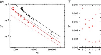
 Re
Re 2ϵ
2ϵ (μ∞,λ,a)=(0,100,2)
 L=1
L=1 n=1
n=1 n=0.8
n=0.8 m=3
m=3 n=0.8
n=0.8 Re=104
 m
m
 ϵ
ϵ m=3
m=3 Cmax=5.99×10⁻⁴
 Cmax=7.03×10⁻⁴
 Cmax=3.50×10⁻⁴

 θ=0
θ=0 Cmax
Cmax Cmax=8.19×10⁻³
 Cmax=8.22×10⁻³
 Cmax=6.90×10⁻³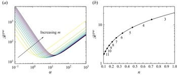
 Rpw
Rpw n=0.8
n=0.8 m=1,2,…,12
 m=3
m=3 Rpw
Rpw Rpw
Rpw n
n m
m
 n=0.5
n=0.5 m=4
m=4 n=0.4
n=0.4 m=5
m=5 n=0.3
n=0.3 m=6
m=6 n=0.25
 m=7
m=7 n=0.2
n=0.2 m=8
m=8
 Uc1
Uc1 Vc1
Vc1 Y=Re1/3(1−r)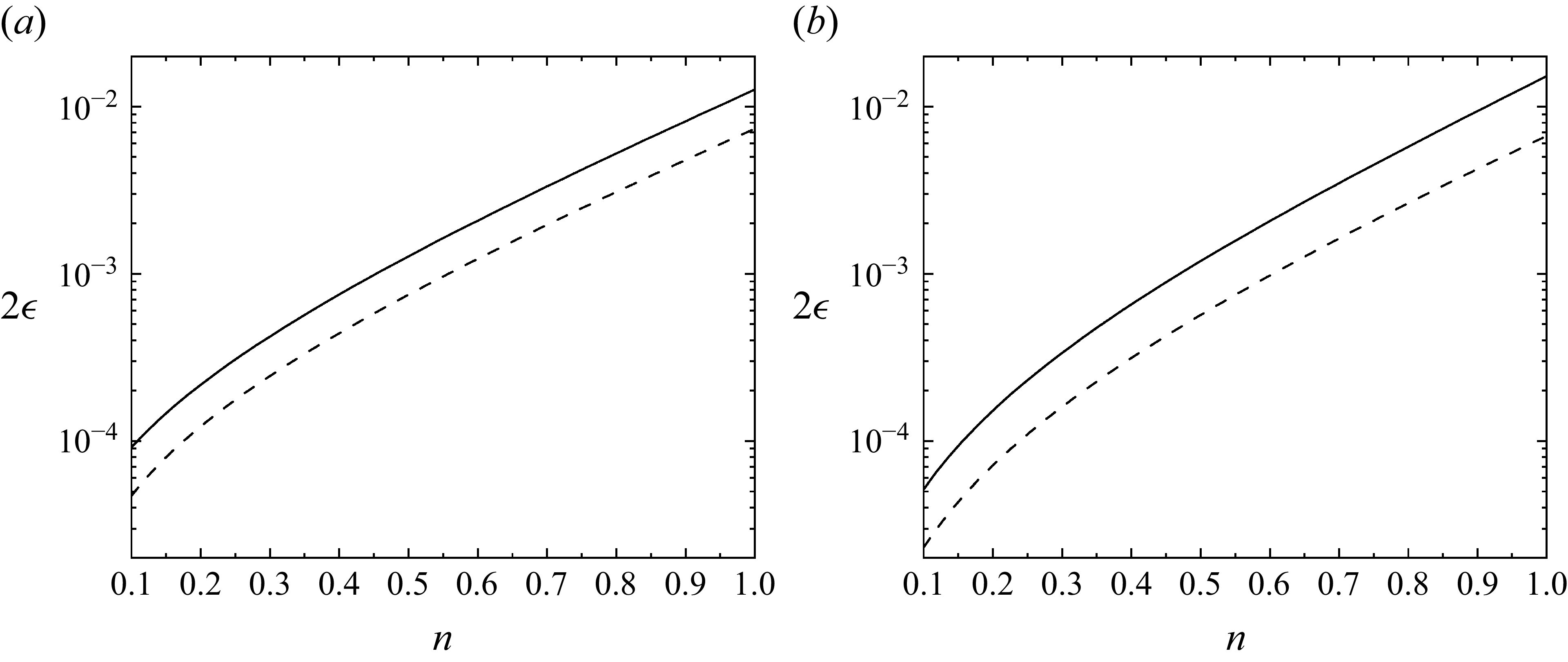
 α
α m
m m=1
m=1 m=5
m=5 ϵ
ϵ λ=100
λ=100 Re=104
 (μ∞,λ,a)=(0,100,2)
 Re=104
 n=0.2
n=0.2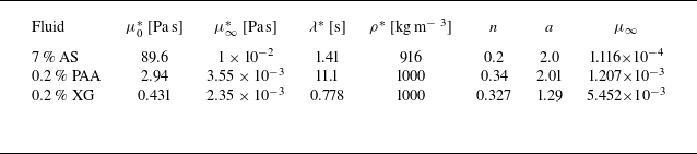
 0.2%
0.2% 0.2%
0.2% ρ∗
ρ∗
 Re=104,λ=100
 a=2
a=2 2ϵ
2ϵ μ∞
μ∞ 10−4
10−4 10−3
10−3 10−2
10−2 m
m α
α m
m n=0.8
n=0.8 α
α m
m
 R∗=0.05
 ϵ
ϵ α
α m
m Reb∈[1.621×105,5.814×105]
 Reb
Reb
 Open access

