


1. Introduction
The depth-limited breaking of surface gravity waves is a beautiful and majestic phenomenon. Wave breaking occurs when Eulerian fluid velocity  $u$ within the wave exceeds the wave phase speed $C$ (e.g. Derakhti et al. Reference Derakhti, Kirby, Banner, Grilli and Thomson2020; Varing et al. Reference Varing, Filipot, Grilli, Duarte, Roeber and Yates2021), typically leading to wave overturning and subsequently the wave jet impacting the sea surface in front of the wave. Wave breaking is often categorized into spilling and plunging breaking (e.g. Peregrine Reference Peregrine1983), where spilling waves have very small overturns, and plunging waves have larger overturns. However, this categorization is qualitative and often identified by sight. In laboratory and field observations, the shape of the wave overturn is important in setting the size of the resulting splash up and bubble entrainment (Chanson & Jaw-Fang Reference Chanson and Jaw-Fang1997; Yasuda et al. Reference Yasuda, Mutsuda, Mizutani and Matsuda1999; Blenkinsopp & Chaplin Reference Blenkinsopp and Chaplin2007), water column turbulence (Ting & Kirby Reference Ting and Kirby1995, Reference Ting and Kirby1996; Aagaard, Hughes & Ruessink Reference Aagaard, Hughes and Ruessink2018), sediment suspension (Voulgaris & Collins Reference Voulgaris and Collins2000; Aagaard et al. Reference Aagaard, Hughes and Ruessink2018) and wave impact forces on engineered structures (Bullock et al. Reference Bullock, Obhrai, Peregrine and Bredmose2007), which may also apply to coastal cliffs (Thompson, Young & Dickson Reference Thompson, Young and Dickson2019). Similarly, in numerical simulations of deep-water and depth-limited wave breaking, the geometry of wave-overturning impacts air entrainment, vorticity generation and pathways of turbulent dissipation (e.g. Lubin et al. Reference Lubin, Vincent, Abadie and Caltagirone2006; Derakhti & Kirby Reference Derakhti and Kirby2014; Deike, Melville & Popinet Reference Deike, Melville and Popinet2016; Mostert & Deike Reference Mostert and Deike2020). Thus understanding the factors that affect the shape of overturning waves is important to a range of processes. Surfers have long understood that offshore (blowing from shore to sea) wind results in larger and more square (1 : 1 aspect ratio) overturns relative to onshore (blowing from sea to shore) wind. Yet this effect of cross-shore wind on overturning wave shape has largely been unstudied. Here, we examine the effect of onshore and offshore wind on field-scale overturning wave shape.
As waves shoal, the shallow-water nonlinearity parameter  $H/h$ increases, where $H$ is the wave height, and $h$ is the water depth. In addition, shoaling waves change shape, becoming steeper with narrower peaks (i.e. skewness) and more pitched forward (i.e. asymmetry) before overturning and breaking (Elgar & Guza Reference Elgar and Guza1985). The nonlinearity parameter is well understood to strongly affect the location of wave breaking (e.g. McCowan Reference McCowan1894; Thornton & Guza Reference Thornton and Guza1983). Wave-overturn shape has been quantified with its area $A$ and its aspect (width to length) ratio $W/L$ (Mead & Black Reference Mead and Black2001), which are known to depend on bathymetric parameters (such as $\beta$, the bathymetric slope) and local nonlinearity parameters ( $H/h$). The parameters $A$,
$A$,  $W$ and $L$ are defined in § 3. In laboratory planar slope settings, $\beta$ is well understood to be important in setting spilling or plunging wave breaking via the Iribarren number (e.g. Peregrine Reference Peregrine1983). Similarly, $\beta$ is also important in setting the overturning wave shape. On a planar beach with $\beta$ varying from 0.01 to 0.067, nearly exact potential flow boundary element model (BEM) solutions reveal that wave-overturn area $A$ increases with $\beta$ for fixed initial soliton amplitude (Grilli, Svendsen & Subramanya Reference Grilli, Svendsen and Subramanya1997). Similar changes to overturn area were also evident with incident solitons on a planar beach in two-phase direct numerical simulations (DNS) modelling with $\beta$ from 0.018 to 0.052 (Mostert & Deike Reference Mostert and Deike2020). Field observations of wave overturns with random waves over a barred beach bathymetry also observed increasing non-dimensional wave-overturn area $A/H_b^2$ (where $H_b$ is the breaking wave height) for larger local $\beta$ varying from 0.02 to 0.026 (O'Dea, Brodie & Elgar Reference O'Dea, Brodie and Elgar2021). The overturn aspect ratio $W/L$ was found to depend somewhat on local $\beta /(kh)$, where $kh$ is the non-dimensional depth based on a peak wavenumber $k$ (O'Dea et al. Reference O'Dea, Brodie and Elgar2021).
Wave-overturn shape also depends on the local nonlinearity parameter  $H/h$, particularly on bars or reefs that have minimum depth at the top of the bar or reef. In BEM simulations of a soliton incident on a step reef (i.e. no slope), the wave-overturn area increased for shallower reefs (larger steps) (Yasuda, Mutsuda & Mizutani Reference Yasuda, Mutsuda and Mizutani1997). Blenkinsopp & Chaplin (Reference Blenkinsopp and Chaplin2008) examined overturning wave shape for laboratory progressive waves over a triangular bathymetry with constant $\beta$ but variable shallowest depth $h_c$ that immediately farther shoreward falls off to deeper water. Non-dimensional wave-overturn area $A/H_b^2$ was proportional to a nonlinearity parameter $H_0/h_c$ where $H_0$ was an deep-water wave height, qualitatively consistent with the step reef of Yasuda et al. (Reference Yasuda, Mutsuda and Mizutani1997). For the triangular bathymetry, no relationship was evident between overturn aspect ratio $W/L$ and nonlinearity parameter $H_0/h_c$ (Blenkinsopp & Chaplin Reference Blenkinsopp and Chaplin2008).
Wind blowing over surface gravity waves leads to wave growth and decay (e.g. Miles Reference Miles1957; Phillips Reference Phillips1957), but can also change the wave shape in both deep (Leykin et al. Reference Leykin, Donelan, Mellen and McLaughlin1995; Zdyrski & Feddersen Reference Zdyrski and Feddersen2020) and shallow (Zdyrski & Feddersen Reference Zdyrski and Feddersen2021) water. Few studies have examined the combined effect of wind and shoaling effects. In laboratory studies, onshore wind results in wave breaking in deeper water (Douglass Reference Douglass1990) and decreases  $H/h$ at breaking (King & Baker Reference King and Baker1996), with the opposite for offshore wind. Numerical studies using two-phase Reynolds-averaged Navier–Stokes (RANS) solvers of wind-forced solitary (Xie Reference Xie2014) and progressive (Xie Reference Xie2017) waves have found results similar to aspects of these laboratory experiments. A parametrized wind energy input within a wave-averaged model can reproduce the changes in wave breakpoint location and $H/h$ at breaking (Sous et al. Reference Sous, Forsberg, Touboul and Gonçalves Nogueira2021). In a laboratory experiment, Feddersen & Veron (Reference Feddersen and Veron2005) demonstrated that stronger onshore wind enhanced the temporal-wave shape (asymmetry) of shoaling waves. Similar wind effects on laboratory shoaling wave skewness and asymmetry were also observed recently (Sous et al. Reference Sous, Forsberg, Touboul and Gonçalves Nogueira2021). Zdyrski & Feddersen (Reference Zdyrski and Feddersen2022) derived a variable coefficient KdV–Burgers equation for a wind-forced soliton shoaling on a planar slope using the Jeffreys (Reference Jeffreys1925) mechanism. Solving this equation numerically, wind direction and speed changed the polarity and magnitude of the induced bound dispersive tail, resulting in wave-shape changes focused on the rear wave face (Zdyrski & Feddersen Reference Zdyrski and Feddersen2022), qualitatively consistent with Feddersen & Veron (Reference Feddersen and Veron2005). However, this study was limited to shoaling well before wave overturning due to the asymptotic limits of the derivation. As normal-stresses (pressure) increase for steeper open-ocean waves, wind-induced effects would likely be even larger for waves near breaking. However, the effects of wind on overturning wave shape have been poorly studied at field scales, due to the difficulties of isolating other influential environment parameters, such as tides, bathymetry, and random and directionally spread wave fields from wind effects. For example, in one field study with natural bathymetric and wave field variations, cross-shore wind was weakly correlated to the overturn aspect ratio, with offshore (onshore) wind increasing (reducing) the aspect ratio (O'Dea et al. Reference O'Dea, Brodie and Elgar2021). However, wind variation was relatively weak, and co-variation with other parameters was not considered. Here, we examine the dependence of the non-dimensional wave-overturn area and aspect ratio on non-dimensional cross-shore wind speed $U_{w}/C$, where $C$ is the wave phase speed, and $U_{w}/C$ is positive for onshore wind. Specifically, we hypothesize larger (smaller) non-dimensional area $A/H^2$ and aspect ratio $W/L$ for increasing offshore (onshore) winds.
Prior to the field study of O'Dea et al. (Reference O'Dea, Brodie and Elgar2021), quantitative wave-overturn shape studies were based on laboratory experiments (e.g. Blenkinsopp & Chaplin Reference Blenkinsopp and Chaplin2008). The rapid transformation of field-scale shoaling to overturning waves requires high temporal and spatial resolution measurements. Advances in using lidar (light detection and ranging) technology to measure surface gravity waves directly (e.g. Brodie et al. Reference Brodie, Raubenheimer, Elgar, Slocum and McNinch2015; Martins et al. Reference Martins, Blenkinsopp, Power, Bruder, Puleo and Bergsma2017, Reference Martins, Blenkinsopp, Deigaard and Power2018; Carini, Chickadel & Jessup Reference Carini, Chickadel and Jessup2021) provide such high-resolution measurements of field-scale waves. Here, we isolate the effect of cross-wave wind on overturning wave shape for field-scale waves on a fixed bathymetry with small variation in incident waves. These observations were made at the Kelly Slater Wave Company's Surf Ranch – a wave basin designed for surfing and used here as a laboratory. In § 2, we describe the fixed bathymetry and waves of the basin, and detail the instrumentation deployed. Analysis methods are detailed in § 3, particularly estimation of wave-overturning parameters. Although coastal wind can blow in any direction relative to wave propagation, we focus on the component of wind in the direction of wave propagation, typically cross-shore (i.e. onshore or offshore) wind. In the results (§ 4), we examine the effect of cross-wave wind on wave breakpoint location, wave-overturn area and aspect ratio, while concurrently examining the effect of a nonlinearity parameter. The context of our results, limitations of our observations, potential mechanisms and implications are discussed in § 5. Section 6 provides a summary.
2. Methods
2.1. Description of the Surf Ranch wave basin
The Surf Ranch wave basin, located in Lemoore, CA, USA, is oriented nearly north to south and is approximately 600 m long and 60 m wide (figure 1a). The bed of the wave basin is fixed (i.e. not mobile). The western side of the basin has a sloping beach. On the eastern side of the basin, northbound and southbound waves are generated by a submerged hydrofoil towed along-basin on a tram. We define a cross- and along-basin  $(x,y)$ coordinate system, with $(x,y)=(0,0)$ located at the centre of the study region, where an instrument frame called ‘the rig’ was deployed (figure 1, black dot). The wave basin bathymetry has a deep flat region on the east side, and shallows towards the west. The bathymetry profile varies along-basin to provide variation in surfing experience. However, in the central study region of the wave basin ( $-35 < y < 35$ m), the bathymetry is along-basin uniform and varies only cross-basin (figure 1b). In the region where waves are generated ( $x>18$ m), the bathymetry is flat with still water depth $h \approx 2.5$ m. A relatively steep sloping section begins at $x \approx 13$ m, which transitions to a flat bar at $x \approx 3$ m that is approximately 6 m wide with
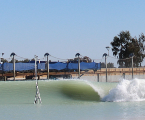
  $h \approx 0.95$ m (figure 1d). Shoreward of the bar is a deeper trough that then transitions into a beach slope even farther shoreward (figure 1d). The bathymetry is designed so that wave overturning occurs on the bar (figure 1), allowing surfers the opportunity to get ‘tubed’ and allowing for the study of field-scale overturning wave shape.
Overview of the Kelly Slater Wave Company's Surf Ranch wave basin. (a) Aerial photo showing the entire basin in Surf Ranch  $(x,y)$ coordinates, with north and south indicated. The black dot shows the location of the rig at $(x,y)=(0,0)$ m, and the orange square shows the location of the meteorological station at $(x,y)=(-50,-73)$ m. The thin black rectangle indicates the centre region of the basin shown in (b,c). (b) Georectified unmanned aerial vehicle (UAV) image of the centre region with a right-wave generated by the submerged hydrofoil towed along-basin by the tram. Bathymetry contours delineate slope, bar, trough and beach slope regions. (c) Georectified UAV image of the centre region with a left-wave. Orange dots indicate subsampled coverage of the Velodyne HDL-32 lidar. (d) Cross-basin transect of Surf Ranch bathymetry at $y=0$.

The hydrofoil is pulled along-basin in a supercritical regime by the tram, generating an approximate soliton with wave height  $H \approx 2$ m together with trailing dispersive waves (figure 1). The soliton propagates at an angle of $25.5^\circ$ to the hydrofoil. Thus, from the perspective of the shoreline, the solitons are highly obliquely ( $\approx 65^\circ$) incident. The solitons propagate up the slope and overturn on the bar (figure 1b,c). Under slowly varying bathymetric conditions, the soliton phase speed would be tied to the wave height and water depth. However, the depth varies rapidly relative to the soliton full width $\approx 6$ m. Projected into the direction of propagation, the water depth is halved over 16 m. The ratio of soliton full width to bathymetric variation distance is 0.38, which is not $\ll 1$. Thus a slowly-varying paradigm does not hold, and the soliton does not have a chance to refract prior to wave overturning. This results in a straight wave crest even though the water depth varies (figure 1b,c). A similar lack of wave refraction over rapidly varying two-dimensional bathymetry was evident in the two-dimensional overturning wave modelling (Guyenne & Grilli Reference Guyenne and Grilli2006). When the hydrofoil is northbound, it generates a northward propagating wave (figure 1b), which from the perspective of an observer (surfer) looking in the direction of wave propagation has open (non-breaking) wave face to the right. Similarly, with the southbound hydrofoil, propagating waves are generated with open face to the left (figure 1c). Here, this surfing convention of right-wave and left-wave will be used to denote northward and southward propagating waves, respectively.
The observation period occurred in March 2019, including the afternoon of 12 March, the afternoon of 13 March, and the morning of 14 March. No surfing occurred during these times. During the observation period, the hydrofoil was pulled at different speed profiles to generate different surfing wave types. Here, we focus on waves that were generated with the same hydrofoil speed profile – denoted CT3 – that had a constant along-basin speed  $C_y \approx 7.4\ \mathrm {m}\ \mathrm {s}^{-1}$ in the study region $-35 < y < 35$ m (figures 1b,c). A basin seiche is induced by the wave generation and breaking. As such, there were intervals of 3–8 min between wave generation, allowing the seiche to reduce. Subtle hydrofoil variations for northbound and southbound waves result in left- and right-waves being slightly different. The hydrofoil was also slightly modified prior to generating waves on 14 March, resulting in slightly larger waves. Thus with seiche, left-wave and right-wave variations, and hydrofoil variations, the CT3 generated waves are not all identical and we must be careful to isolate the effects of cross-wave wind against nonlinearity (variation in the size of generated waves) and bathymetric (seiching changing the depth of the bar) induced changes to overturning wave shape.
2.2. Instrumentation and data
2.2.1. Ground-based images
At each end of the wave basin, an automated camera system takes video of each wave, from which we extract still images. These images provide qualitative information about each wave. Example images of a left- and right-wave approaching  $(x,y)=(0,0)$ m are shown in figures 2(a,b).
Overview of (a,c,e) a left-wave and (b,d, f) a right-wave. (a,b) Ground-based photograph of oncoming wave just prior to arrival at the rig (vertical pole extending from the water). The magenta diamond indicates the approximate breakpoint location where the overturning lip impacts the wave face, resulting in a splash up. (c,d) Wave staff water level  $\eta$ versus time $t$. The blue circle represents the maximum of $\eta$, and the vertical grey bar represents the wave staff wave height $H$. Note that the mean pre-wave water levels were $-0.03$ m and $-0.007$ m, respectively. (e, f) Georectified aerial image in $(x,y)$ coordinates as the wave is approaching the rig at $(x,y)=(0,0)$ m, with overlaid lidar returns (colour indicates elevation, no scale).

2.2.2. UAV-based images
A DJI Phantom 4 Pro unmanned aerial vehicle (UAV) was used to take videos of the waves as they pass the rig. The UAV was flown at elevation 120 m above the water surface. Videos were taken in 4K (3840 by 2160 pixels at 30 frames per second). Images were extracted from the videos at 5 Hz centred on the rig, georectified using a flat plane at the still-water elevation in NAVD88 using multiple ground-control points following Bruder & Brodie (Reference Bruder and Brodie2020), and put into the  $(x,y)$ coordinate system (figures 1b,c and 2e, f). Georectified images have spatial resolution $({\rm \Delta} x,{\rm \Delta} y) \approx 0.05$ m.
2.2.3. Wave staff deployed at rig
A tripod (denoted the ‘rig’) was deployed at  $(x,y)=(0,0)$ about 20 m from the mean shoreline in the centre of the flat bar region (black dot in figure 1b). The still-water level at the tripod is on average 0.95 m. An Ocean Sensor Systems OSSI-010-025 Wave Staff XB was mounted on the tripod that sampled at 32 Hz and communicated over a wireless network with occasional drop outs. The wave staff is calibrated so that the still-water depth is known. Only waves with wave staff data were included in the analysis. Based on image data, waves that were clearly broken prior to encountering the wave staff were not included. Time series of wave staff water level $\eta (t)$ characteristically have a rapidly growing front face and a slower receding back face consistent with shoaling-induced increase in wave asymmetry (figures 2c,d). Wave arrival times were estimated as the first maximum in the wave staff data (see blue circle in figure 2c,d). For each wave, pre-wave water levels are estimated from a 1 s-long time average of $\eta (t)$, from 3.75 s to 2.75 s prior to wave arrival. The wave height $H$ is estimated as $\eta$ at the arrival time minus the pre-wave water level (grey bars in figures 2c,d). The pre-wave water depth $h$ is the pre-wave water level plus the still-water depth.
2.2.4. Lidar deployed at rig
Three-dimensional snapshots of the water surface are generated with a Velodyne HDL-32 lidar that was deployed on top of a vertical pole attached to the rig at  $(x,y)=(0,0)$ m at elevation 4.05 m above the still-water surface. The HDL-32 lidar has 32 beams with 903 nanometre wavelength scanning at 10 Hz, and was configured similar to that of O'Dea et al. (Reference O'Dea, Brodie and Elgar2021). Lidar returns from this sensor have a typical accuracy of $\pm 0.02$ m. The lidar is oriented largely in the $y$ direction to map the front face of the wave as it shoals and overturns (figure 1c). For a typical single wave, the $(x,y)$ extent of all lidar returns ranges up to $\pm 20$ m from the rig (figure 1c). The 32 lidar beams are spaced at $1.33^\circ$ increments, yielding a $41^\circ$ field of view. Thus the cross-basin extent of the scans increases with along-basin distance from the lidar, from $\approx 5$ m at $|y|=5$ m to $\approx 13$ m at $|y| = 15$ m (figure 1c). Similarly, the cross-basin resolution varies from ${\rm \Delta} x \approx 0.12$ m at $|y|=5$ m to ${\rm \Delta} x \approx 0.4$ m at $|y|=15$ m. The azimuthal (along-basin) resolution is very high at $0.166^\circ$, equivalent to ${\rm \Delta} y \approx 0.01$ m at $|y|=15$ m. The extent of quality returns depends on the incident beam angle to the water surface, distance from the lidar, water roughness, and foam. As the lidar rotates $360^\circ$ at 10 Hz, a snapshot of the wave is obtained over 0.1 s. Example lidar snapshots for a left- and right-wave are consistent with drone-based image observations (figures 2e, f).
2.2.5. Wind measurements
An AIRMAR PB100 meteorological station was mounted at elevation 16 m above the still-water level on the beach side just outside the basin at  $(x,y)=(-50,-73)$ m (orange square in figure 1a). The cross- and along-basin winds in the ( $x,y$) coordinate system ( $u_w,v_w$) were sampled at 1 Hz, with occasional gaps interpolated linearly. Wind time series were then low-pass filtered with a 0.033 Hz cutoff frequency. On 12 and 13 March, the winds were mostly from the north-northwest (i.e. $u_w>0$ and $v_w<0$) at speeds generally 3–7 $\mathrm {m}\ \mathrm {s}^{-1}$. On 14 March, the winds were weaker (between 0.5–2 $\mathrm {m}\ \mathrm {s}^{-1}$) out of the south-southwest. For each wave, the wind values were estimated from the low-pass filtered wind at the rig wave arrival time (blue dot in figures 2c,d). No correction was made for the altitude of the wind measurements. Although a row of trees is present near the shore side of the wave basin in $-125 < y < 350$ m, we also assume no wind veering in the vertical. Analysis results are similar if only the along-basin component is used and the cross-basin component is set to zero.
3. Analysis
Here, we focus on the CT3 waves during the observational period that had data from the wave staff, UAV, Velodyne lidar and meteorological station. Occasionally, waves overturn and break at  $x>0$ (east of the wave staff), as determined from both ground-based and aerial images. These waves typically correspond to conditions when strong seiching was still present in the basin. Thus we also remove these waves from consideration, resulting in 22 total waves (11 left-waves and 11 right-waves).
3.1. UAV image breakpoint
The breakpoint location  $(x_{{bp}},y_{{bp}})$ is defined as where the overturning wave lip impacts the water surface creating a splash up of ‘white water’ (magenta diamonds in figures 2a,b). Breakpoint locations are identified by eye from georectified UAV images where the ‘white water’ splash origination location is clearly evident (figure 3). Breakpoint locations are determined within a 20 m along-basin region up-wave of the rig (at $(x,y)=(0,0)$ m), so that any rig wake effects are not included. For a left-wave, the breakpoints $(x_{{bp}},y_{{bp}})$ for four images, each separated by 1 s, are shown as solid red dots in figure 3(a), with the $(x_{{bp}},y_{{bp}})$ from images in between indicated as red $\times$ symbols. Breakpoints for a right-wave are shown in figure 3(b). The $x_{{bp}}$ vary weakly along-basin with variance $0.11\ \mathrm {m}^2$ averaged over all 22 waves. For each wave, a single cross-basin breakpoint location $X_{{bp}}$ is estimated as an along-basin average of $x_{{bp}}$ for each $y_{{bp}}$ located within 20 m up-wave of the rig, implying an averaging region $0 \le y_{{bp}} \le 20$ m or $-20 \le y_{{bp}} \le 0$ m for a left-wave or right-wave, respectively. As along-basin wave speeds are 7.4 $\mathrm {m}\ \mathrm {s}^{-1}$, and UAV images are at 5 Hz, the along-basin average $X_{{bp}}$ includes 12 $x_{{bp}}$ locations for each wave. The standard error of $X_{{bp}}$ is $0.10$ m, assuming independent estimates from each image. For all waves, $X_{{bp}}$ is shoreward of the rig. The mean $X_{{bp}}$ over all 22 waves is $\bar {X}_{{bp}} = -2.83$ m. For each wave, the perturbation cross-shore breakpoint is defined as $\Delta X_{{bp}} = X_{{bp}} - \bar {X}_{{bp}}$. The still-water shoreline is located at $x_{sl}=-20$ m. Thus the mean surf zone width (breakpoint distance from the mean shoreline) is $\bar {L}_{sz} = |\bar {X}_{{bp}} - x_{sl}|$, which is used to non-dimensionalize $\Delta X_{{bp}}$ in the results that follow.
Breakpoints  $(x_{{bp}},y_{{bp}})$ (red markers) over UAV greyscale wave image slices for (a) the left-wave and (b) the right-wave shown in figure 2. Sequential image slices are at 1 Hz with associated $(x_{{bp}},y_{{bp}})$ (solid red circles). The $(x_{{bp}},y_{{bp}})$ at 5 Hz in between the 1 Hz images are denotes with red $\times$ symbols. Image slices are taken at $\pm 25.5^{\circ }$ (right- and left-wave, respectively) with respect to $x$ associated with the wave coordinate system $(\tilde {x},\tilde {y})$ with origin $(\tilde {x},\tilde {y})=(0,0)$ m also at the rig. Each individual image slice is 8 m wide in $y$ and centred at $y_{{bp}}$.

3.2. Visualizing wave overturns from lidar
For analysis of wave overturns, each lidar snapshot is rotated into a wave coordinate system as in O'Dea et al. (Reference O'Dea, Brodie and Elgar2021), where  $(\tilde {x},\tilde {y})$ are in the wave propagation and along-wave directions, respectively, with $+\tilde {y}$ directed towards the tram where waves are generated, and origin $(\tilde {x},\tilde {y})=(0,0)$ m at the rig (see figure 3), which is also the origin of the $(x,y)$ coordinate system. As discussed in § 2.1, the rapid bathymetric variations prevent soliton refraction, resulting in straight wave crests with a consistent angle of $25.5^\circ$ relative to the $x$ direction (figure 3). Thus, the $(\tilde {x},\tilde {y})$ coordinate system is rotated $115.5^\circ$ either clockwise (left-waves) or counter-clockwise (right-waves) from the $(x,y)$ coordinate system. For right-waves, the $\tilde {y}$ axis is flipped (figure 3), resulting in a left-handed coordinate system. Thus both left- and right-waves have the breakpoint propagating in the $+\tilde {x}$ and $+\tilde {y}$ directions (figure 3). In the rotated wave coordinate system, left- and right-wave overturns are well captured by lidar snapshots (figure 4), as $-\tilde {y}$ directed views look directly into the overturn. For each wave, the wave coordinate system is fixed. Here, $z$ is the vertical coordinate, with $z=0$ m at the still-water level prior to the wave.
Visualizations of lidar snapshot returns in wave coordinates ( $\tilde {x},z$) of (a,c,e) the left-wave and (b,d, f) the right-wave shown in figures 2 and 3. The rows show three snapshots separated by $0.3$ s each. Colours indicate along-wave distance $\tilde {y}$ as defined in figure 3. The grey diamonds indicate the mid-wave-face locations $\tilde {x}_{{wf}}$.

We highlight a few points for a left-wave and a right-wave as the waves propagate through the lidar field of view. For these obliquely incident waves (figures 2a,b), along-wave ( $\tilde {y}$) variations from the wave face (larger $\tilde {y}$) to the overturn (smaller $\tilde {y}$) are visualized clearly (colours in figure 4). Here, the wave-overturn shape is quasi-uniform in time (snapshots, or successive rows in figure 4). As the wave propagates in the $+\tilde {x}$ direction, it also moves in the $+\tilde {y}$ direction (colours get darker in time, figure 4) as the wave breakpoint $x_{{bp}}$ is essentially constant in $y$ (figure 3). The density of lidar returns increases for smaller $|\tilde {x}|$ as the wave is closer to the rig, but the $\tilde {y}$ range (swath) also decreases (see also figure 1c). This left-wave is consistently at larger $\tilde {y}$ than the right-wave (figure 4) as the left-wave overturns at larger cross-basin $x$ than the right-wave. Thus more of the wave face is visualized for the right-wave. Spray is observed clearly shedding off of the back of the right-wave (dots above $z=2.5$ m, figure 4), which is not seen for the left-wave. The location of the mid-wave-face $\tilde {x}_{{wf}}$ is defined as the median $\tilde {x}$ for lidar returns at $0.95 < z < 1.05$ m. For each wave snapshot, the estimated $\tilde {x}_{{wf}}$ (grey diamonds in figure 4) represents well the $\tilde {x}$ location halfway up the wave face. To ensure sufficient lidar resolution and swath, we limit analysis of wave overturns to $\tilde {x}_{{wf}}$ between $-8$ m and $-3$ m.
The quasi-uniformity of the wave overturn across lidar snapshots (figure 4) together with the lack of soliton refraction (figures 1 and 3) implies that for a single snapshot, we can use the  $\tilde {y}$ direction as a proxy for time. The along-basin hydrofoil (wave) speed $C_y = 7.4\ \mathrm {m}\ \mathrm {s}^{-1}$ and wave angle $25.5^{\circ }$ yield $\tilde {x}$ wave propagation speed $C=6.68\ \mathrm {m}\ \mathrm {s}^{-1}$ and $\tilde {y}$ propagation speed $C_{\tilde {y}}=3.19\ \mathrm {m}\ \mathrm {s}^{-1}$. Thus at a fixed time, moving an along-wave ( $\tilde {y}$) distance 3.19 m is equivalent to 1 s of temporal wave evolution. A single lidar snapshot of the right-wave in figure 4 is binned in $\tilde {y}$ to demonstrate how the time evolution of wave overturning can be visualized (figure 5). Lidar returns are separated into ${\rm \Delta} \tilde {y}=2$ m wide bins, with bin-centres $\tilde {y}_{c}$ sliding over every 0.9 m varying from $\tilde {y}_{c}=-1.7$ m to $-6.2$ m (figure 5). The 4.5 m variation in $\tilde {y}_{c}$ corresponds to 1.4 s in time evolution, highlighting the rapid spatio-temporal evolution of such overturning waves. The ${\rm \Delta} \tilde {y}=2$ m bin width ensures a sufficient number of points for visualization, and contains $0.63$ s of wave evolution. With this bin width, lidar returns can overlap across bins. Nearest the tram ( $\tilde {y}_{c} = -1.7$ m, figure 5a), the wave face has not yet become vertical. Moving towards the overturn, the wave face is vertical at $\tilde {y}_{c}=-2.6$ m (figure 5b). At $\tilde {y}_{c}=-3.5$ m, the wave jet (lip) forms, ejecting forwards (figure 5c). At $\tilde {y}_{c}=-4.4$ m, the wave is overturning with jet falling forwards (figure 5d). At $\tilde {y}_{c} = -5.3$ m, the wave jet has fallen about 1.5 m in $z$ and nearly makes contact with the water surface (figure 5e), about $+2$ m (in $\tilde {x}$) from where the wave became vertical. In this bin, most of the overturn surface (wave face, upper-back, bottom of the jet) is visible. Farther shoreward at $\tilde {y}_{c} = -6.2$ m, the jet has impacted and the overturn surface is obscured from view (figure 5f).
Visualizations of lidar snapshot returns in wave coordinates ( $\tilde {x},z$) of the right-wave in figure 4 for ${\rm \Delta} y=2$ m wide bins at bin-centres $\tilde {y}_{c}$ separated by 0.9 m from (a) most positive $\tilde {y}_{c}$ (nearest wavemaker) to ( f) most negative $\tilde {y}_{c}$ (nearest shoreline). The six panels cover 1.4 s of time evolution. Colours represent $\tilde {y}$. Each ${\rm \Delta} y=2$ m wide bin contains 0.63 s of time evolution.

3.3. Projecting the wind vector into the wave propagation direction
For each wave, the wind speed ( $U_{w}$) in the direction of wave propagation was estimated as the dot product of the wind vector with the unit wave direction vector $\tilde {\boldsymbol {x}}$ (figure 3). Thus $U_{w}<0$ for offshore wind (in the opposite direction of wave propagation) and $U_{w}>0$ for onshore winds (in the direction of wave propagation). The non-dimensional wind speed in the direction of wave propagation $U_{w}/C$ uses the wave speed in the direction of wave propagation $C=6.68\ \mathrm {m}\ \mathrm {s}^{-1}$, and will be used in subsequent analysis. The range of $U_{w}/C$ spans from $-1$ to $0.7$. This range can be contextualized by considering ocean waves breaking in $h=2.5$ m depth. For such waves, $C \approx 5\ \mathrm {m}\ \mathrm {s}^{-1}$, implying realistic cross-wave wind speed variation from $-5\ \mathrm {m}\ \mathrm {s}^{-1}$ to $+3.5\ \mathrm {m}\ \mathrm {s}^{-1}$.
3.4. Estimating wave-overturning shape parameters
To extract overturn parameters such as area and aspect ratio, we fit lidar returns to a functional form representing an overturn. A parametric function based on cubic free-surface potential flow solutions (Longuet-Higgins Reference Longuet-Higgins1982) is used to fit the shape of the wave overturn. The functional form is
 \begin{equation} \frac{z'}{W} ={\pm} \frac{ 3\sqrt{3}}{4} \sqrt{\frac{x'}{L}}\left(\frac{x'}{L}-1\right), \end{equation}
where the  $x'$ and $z'$ coordinates are oriented along and across the overturn, and $L$ and $W$ are the overturn length and width, respectively (figure 6a). With (3.1), the region near $x'=0$ is the back of the overturn (red and green, figure 6a), and the region near $x' =2$ is where the overturning jet (magenta) intersects the water surface in front of the wave (brown). Parameters derived from $W$ and $L$ that will be analysed are the overturn area
 \begin{equation} A = \frac{2\sqrt{3}}{5}\,LW, \end{equation}
and the aspect ratio  $W/L$. When rotated clockwise by an angle $\theta$, the curve of the functional form (6a) is qualitatively similar to the shape of the overturn seen in figures 4 and 5. The functional form (3.1) has been used successfully to fit wave-overturning shape parameters from images of random waves breaking on reefs (Mead & Black Reference Mead and Black2001), laboratory visualizations of plunging waves (Blenkinsopp & Chaplin Reference Blenkinsopp and Chaplin2008), and field lidar observations of plunging breaking waves (O'Dea et al. Reference O'Dea, Brodie and Elgar2021). As noted by O'Dea et al. (Reference O'Dea, Brodie and Elgar2021), (3.1) is only a potential flow solution when the overturn aspect ratio is $W/L = 0.36$ (Longuet-Higgins Reference Longuet-Higgins1982). However, as pointed out by New (Reference New1983), this solution does not give the correct surface velocity for an overturn. Thus, as in previous work (Blenkinsopp & Chaplin Reference Blenkinsopp and Chaplin2008; O'Dea et al. Reference O'Dea, Brodie and Elgar2021), the functional form (3.1) should be considered as means of quantifying wave-overturn shape and reducing it to two parameters, $L$ and $W$.
$W$.
Schematic of overturn shape fitting. (a) The overturn curve from the Longuet-Higgins (Reference Longuet-Higgins1982) functional form (3.1) as a function of  $x'$ and $z'$ for overturn length $L=2$ m and width $W=0.7258$ m, indicated with thick grey lines. Specific overturning regions are indicated in colour, including the upper-back (red) and lower-back (green) parts of the overturn at $x'\approx 0$, and at $x\approx L$, the overturning jet (magenta) impacting the water surface in front of the wave face (brown). (b) Example of the fitting method: lidar returns (coloured dots) as a function of $\tilde {x}$ and $z$ of the ${\rm \Delta} \tilde {y}=2$ m region from figure 5 with the fit curve of (3.1). Black dots represent the fit-lidar returns. The thick grey lines represent the best fit $L=2.32$ m and $W=1.07$ m with other best-fit parameters $\theta =35^\circ$ (indicated in (b)), and $(\tilde {x}_0,z_0)=(-4.41,1.60)$ m is the location of the back of the overturn. Note that the overturn has five fit-returns near the upper-back of the overturn (red), and $\ge 15$ fit-returns in the jet (magenta) and front-face region (green), indicating that this is a fit-snapshot.

For each lidar snapshot, we first select the  ${\rm \Delta} \tilde {y} =2$ m wide binned region to fit to this functional form. We require the binned region to have returns that visualize most of the overturn surface and have the jet impacting or nearly impacting the water surface in front of the wave. Such a binned region is denoted as having a complete overturn. Thus the binned regions in figures 5(a–d) do not qualify, as the jet is neither formed nor about to make impact. The binned region in figure 5( f) also does not qualify, as the back of the overturn (i.e. $(x',z')=(0,0)$) is not visible. For this lidar snapshot, only the ${\rm \Delta} \tilde {y}=2$ m region shown in figure 5(e) qualifies as a candidate for fitting because it is the ${\rm \Delta} \tilde {y}$ region with most positive $\tilde {y}_{c}$ with a complete overturn.
The method of fitting the lidar returns to (3.1) is similar that used by O'Dea et al. (Reference O'Dea, Brodie and Elgar2021) and illustrated in figure 6(b) for the binned lidar returns in figure 5(e). There are five fit parameters ( $L,W,\theta,\tilde {x}_0,z_0$), where $\theta$ is the clockwise rotation angle of the overturn major axis to the horizontal, and ( $\tilde {x}_0,z_0$) corresponds to $(x',z')=(0,0)$, that is, the back of the overturn. The fit process is iterative. The first step is to fit all the binned lidar returns (coloured dots in figure 6b) to the parametric form of (3.1) yielding the first set of best-fit parameters. For the $i$th lidar return, $d_i$ is defined as the minimum Euclidean distance from the lidar return to the fit-curve (3.1). The best-fit parameters are those that minimize the cost function of the mean square minimum distance averaged over all lidar returns $\langle d^2 \rangle$. This minimization is performed with a Nelder–Mead unconstrained simplex search method (Press et al. Reference Press, Flannery, Teukolsky and Vettering1988; Lagarias et al. Reference Lagarias, Reeds, Wright and Wright1998). An initial parameter guess is needed, with $L$ and $W$ chosen larger than the largest overturn, $\theta =40^\circ$, and $(\tilde {x}_0,z_0)$ based on $\tilde {x}_{{wf}}$ and $H$. Next, as we seek to fit to lidar returns from the overturn surface, individual lidar returns are pruned based on their $d_i$ values. Specifically, returns outside the curve with $d_i> 0.08$ m and returns inside the curve with $d_i> 0.4$ m are pruned. Remaining lidar returns are considered the fit returns. The fitting and pruning procedures are repeated using the previous best-fit parameters as initial guess until the best-fit parameters converge and the number of fit returns converges. For the binned region of figure 5(e) (reproduced in figure 6b), the fit curve and associated fit-lidar returns (curve and black dots in figure 6(b), respectively), capture the overturn shape well.
The lidar returns are not distributed uniformly along the overturn curve (figure 6b). In particular the upper-back (red, figure 6), lower-back (green), jet (magenta) and impacting front-face (brown) regions typically have fewer lidar returns, whereas the blue regions (figure 6) typically have more lidar returns. Having unsampled regions of the curve can bias the fit parameters. To prevent this, additional constraints are applied. First, we require the number of fit-lidar returns  $n_{{fit}}> 150$. Second, we require that specific regions of the overturn curve have lidar returns associated with them. We require at least eight lidar returns associated with the front-face and lower-back regions (brown and green, respectively, in figure 6). We also require at least three lidar returns associated in the impacting jet region (magenta) and the upper-back of the overturn (magenta and red in figure 6), regions that typically have fewer returns. For example, the fit in figure 6(b) has five lidar returns associated with the upper-back of the overturn. Overall, there were 70 fit-snapshots across the 22 waves.
For a complete overturn, the fit process is robust and the overturn shape is well captured by the fit for many wave lidar snapshots. In figure 7, two left-wave and two right-wave examples of fit-snapshots are shown with the fit-overturn curve and fit-lidar returns applied to the  ${\rm \Delta} \tilde {y}=2$ m region defining a complete overturn. For these examples, fit-lidar returns are sufficient in the lower-back, upper-back and jet regions (corresponding to green, red and magenta regions, respectively, of figure 6) of the overturn. These fit-snapshot examples (figure 7) also highlight qualitatively how cross-wave wind may affect overturning wave shape. For both left- and right-waves in offshore wind conditions ( $U_{w}/C<0$), the fits give a relatively large aspect ratio $W/L \approx 0.5$ (figures 7a,b) and larger dimensional overturn area $A = 1.74~\mathrm {m}^2$. In contrast, the onshore wind ( $U_{w}/C>0$) cases have smaller aspect ratios $W/L \approx 0.35$ and smaller $A \approx 1.47~\mathrm {m}^2$ than those for offshore winds. In all four cases, the fit $\theta$ was within $\pm 2^\circ$ of $\theta =40^\circ$.
Examples of lidar snapshot returns (colours representing  $\tilde {y}$) as a function of $\tilde {x}$ and $z$ with fit-lidar returns (black) within the ${\rm \Delta} y=2$ m wide region of the complete overturn and the fit-overturn curve (grey dashed). Thick grey lines represent $L$ and $W$. (a,c) Left-waves and (b,d) right-waves for (a,b) offshore wind conditions $U_{w}/C = \{ -0.18,-0.76\}$, and (c,d) onshore wind conditions $U_{w}/C = \{0.60,0.07\}$. The wave-overturning shape parameters are (a) $A=1.74~\mathrm {m}^2$, $W/L=0.51$; (b) $A=1.74~\mathrm {m}^2$, $W/L=0.49$; (c) $A=1.46~\mathrm {m}^2$, $W/L=0.35$; (d) $A=1.47~\mathrm {m}^2$, $W/L=0.36$. For all four panels, $\theta$ is within $\pm 2^\circ$ of $40^\circ$.

This fitting process is applied for each lidar snapshot of each wave where  $-8 < \tilde {x}_{{wf}} < -3$ m. Each lidar snapshot is binned into ${\rm \Delta} \tilde {y}=2$ m wide bins (e.g. figure 5) with bin centres $\tilde {y}_{c}$ moving over every 0.3 m, corresponding to roughly $0.1$ s of wave evolution. Smaller ${\rm \Delta} \tilde {y}$ regions result in fewer fit-snapshots, and larger ${\rm \Delta} \tilde {y}$ result in more aliasing of temporal wave evolution. The fit method is applied to the $\tilde {y}_{c}$ bins that capture a complete overturn (e.g. figure 5e). If multiple $\tilde {y}_{c}$ binned regions are considered fit-snapshots, then the most positive $\tilde {y}_{c}$ bin is used. For the 22 waves, the average number of fit-snapshots was 3.2. Four waves had only one fit-snapshot, three waves had two fit-snapshots, and the rest had more than three fit-snapshots. For each wave, mean area $A$ (3.2) and mean aspect ratio $W/L$ are estimated by averaging parameters across all fit-snapshots. For waves with $\ge 2$ fit-snapshots, we also calculate standard errors of $A$ and $W/L$ from their standard deviations ( $\sigma _A,\sigma _{W/L}$) divided by $\sqrt {n-1}$.
4. Results
Here, we re-state the hypotheses to be examined. We have three non-dimensional wave-overturning parameters: breakpoint location  $\Delta X_{{bp}}/\bar {L}_{sz}$, area $A/H^2$, and aspect ratio $W/L$. As discussed in § 1, increasing the nonlinearity parameter $H/h$ is known to increase $\Delta X_{{bp}}/\bar {L}_{sz}$ (McCowan Reference McCowan1894) as well as increasing $A/H^2$ (Blenkinsopp & Chaplin Reference Blenkinsopp and Chaplin2008). Onshore (offshore) winds $U_{w}/C$ are also understood to increase (decrease) $\Delta X_{{bp}}/\bar {L}_{sz}$ for laboratory waves (e.g. Douglass Reference Douglass1990; King & Baker Reference King and Baker1996). Cross-wave winds may also affect $W/L$ (O'Dea et al. Reference O'Dea, Brodie and Elgar2021). Here, the observations of field-scale wave overturning on a fixed bathymetry are used to test the following hypotheses.
(i) Offshore (onshore) $U_{w}/C$ results in smaller (larger) $\Delta X_{{bp}}/\bar {L}_{sz}$ .
(ii) Offshore (onshore)
$U_{w}/C$ leads to larger (smaller) $A/H^2$.(iii) Offshore (onshore)
$U_{w}/C$ leads to larger (smaller) $W/L$.


To test these hypotheses, we will decouple the effects of  $U_{w}/C$ and $H/h$ in these field-scale observations.
4.1. Relationships between the dimensional and non-dimensional parameters
First, we review the dimensional parameters (e.g. wave staff wave height  $H$ and pre-wave water depth $h$) and the non-dimensional parameters ( $U_{w}/C$ and $H/h$) governing the 22 waves (11 left-waves and 11 right-waves) as shown in figure 8. For all the waves, the pre-wave water depth $h$ varies between 0.91 m and 0.99 m, due to minor seiching, with no significant difference between left- and right-waves (figure 8a). The wave staff wave height $H$ varied between 1.97 m and 2.33 m, with left-waves typically larger than right-waves (figure 8a). On 14 March, waves were slightly larger due to a small modification to the hydrofoil. No systematic relationship between $H$ and $h$ is evident, either for all waves (correlation $r=-0.03$) or for left-waves ( $r=0.13$) and right-waves ( $r=0.21$) in isolation. Thus wave height variations are not linked to seiching-induced pre-wave water depths.
Wave and cross-wave wind parameters for the 22 analysed waves. (a) Wave staff wave height  $H$ versus still-water depth $h$, and (b) nonlinearity parameter $H/h$ versus $U_{w}/C$. Red circles and blue diamonds represent left- and right-waves, respectively. In (a), the correlation between $h$ and $H$ is ${r=\{0.13, 0.21, -0.03\}}$ for left-waves, right-waves and all waves. In (b), the correlation between $U_{w}/C$ and $H/h$ is $r=\{{\bf -0.71}, {\bf 0.75}, {\bf 0.42}\}$ for left-waves, right-waves and all waves. For reference, the 95 % significance level for correlation is $0.52$ for the left- or right-waves, and $0.36$ for all waves. Correlations significantly (95 % level) different from zero are indicated in bold here and in the captions for figures 9, 10 and 12.

Non-dimensional perturbation breakpoint location  $\Delta X_{{bp}}/\bar {L}_{sz}$ versus (a) non-dimensional cross-wave wind speed $U_{w}/C$, and (b) nonlinearity parameter $H/h$. Red circles and blue diamonds represent left- and right-waves, respectively. The magenta dashed line at $\Delta X_{{bp}}/\bar {L}_{sz} = 0.1523$ is the location of the rig. In (a), the thick black lines highlight zero values of abscissa and ordinate. Also, the correlations between $U_{w}/C$ and $\Delta X_{{bp}}/\bar {L}_{sz}$ are $r=\{{\bf 0.64}, {\bf 0.85}, {\bf 0.83}\}$ for left-waves, right-waves and all waves. In (b), the correlations between $H/h$ and $\Delta X_{{bp}}/\bar {L}_{sz}$ are $r=\{-0.45, {\bf 0.54}, {\bf 0.49}\}$ for left-waves, right-waves and all waves. Correlations significantly (95 % level) different from zero are indicated in bold (see figure 8). Note that the standard error of $\Delta X_{{bp}}/\bar {L}_{sz}$ is 0.006, which is very small relative to the variation of $\Delta X_{{bp}}/\bar {L}_{sz}$.

Non-dimensional wave-overturn area ( $A/H^2$) and aspect ratio $W/L$ versus (a,c) non-dimensional cross-wave wind speed $U_{w}/C$, and (b,d) $H/h$. Blue diamonds and red circles represent left-waves and right-waves, respectively. The symbol is the mean, and the error bar represents the standard error. The four smaller symbols represent the waves with only one fit-snapshot. The correlations between $A/H^2$ and $U_{w}/C$ are $r=\{ {\bf -0.75}, {\bf -0.64}, {\bf -0.83}\}$ for left-waves, right-waves and all waves, whereas between $A/H^2$ and $H/h$ they are $r=\{ {\bf 0.67}, {\bf -0.59}, {\bf -0.45}\}$. For $W/L$, its correlations with $U_{w}/C$ and $H/h$, respectively, are $r=\{ {\bf -0.61}, {\bf -0.80}, {\bf -0.77}\}$ and $r=\{ {\bf 0.53}, -0.49, -0.25\}$ for left-waves, right-waves and all waves. Correlations significantly (95 % level) different from zero are indicated in bold (see figure 8).

The non-dimensional cross-wave wind speed  $U_{w}/C$ varies from $-1.2$ to 0.7 (figure 8b), with right-waves preferentially having offshore wind conditions (negative $U_{w}/C$), and left-waves having preferentially onshore wind (positive $U_{w}/C$). This is due to the predominantly north-northwest wind on 12 and 13 March, which is oriented onshore for left-waves and offshore for right-waves. On 14 March, the wind was mostly southerly but weak, thus there were five left-waves that had slightly ( $U_{w}/C \approx -0.2$) offshore wind, and two right-waves with slightly onshore wind ( $U_{w}/C \approx 0.2$, figure 8b). This $U_{w}/C$ range is smaller than the $U_{w}/C \approx \pm 5$ of laboratory experiments (Douglass Reference Douglass1990; King & Baker Reference King and Baker1996).
We next examine the relationship between  $H/h$ and $U_{w}/C$ (figure 8b), which is needed to decouple their effects on the non-dimensional wave-overturning parameters. The overall $H/h \approx 2.25$ is large, indicating that the waves are shortly to overturn. The $H/h$ value varies weakly between 2.05 and 2.57, a factor of 4 smaller relative to the range observed in Blenkinsopp & Chaplin (Reference Blenkinsopp and Chaplin2008). For the left-waves, $H/h$ is negatively correlated ( $r=-0.72$) with $U_{w}/C$. As smaller $H/h$ would lead to smaller $A/H^2$ (Blenkinsopp & Chaplin Reference Blenkinsopp and Chaplin2008), and larger $U_{w}/C$ is also hypothesized to lead to smaller $A/H^2$, this negative $U_{w}/C$ and $H/h$ correlation implies that decoupling $A/H^2$ dependence for left-waves requires care. The right-waves have $H/h$ positively correlated ( $r=0.75$) with $U_{w}/C$. This positive correlation makes it easier to separate $U_{w}/C$ and $H/h$ effects on wave-overturning parameters. Note that these $H/h$ and $U_{w}/C$ correlations are significantly different from zero (figure 8b) but do not imply causation. These $U_{w}/C$ and $H/h$ correlations and anti-correlations for left- and right-waves are largely due to the different wind and wave generation conditions on 14 March. For all waves, the $H/h$ and $U_{w}/C$ relationship is less clear, with weaker correlation $r=0.42$.
4.2. Non-dimensional breakpoint location
We now examine the effect of the non-dimensional cross-wave wind speed  $U_{w}/C$ and the nonlinearity parameter $H/h$ on the non-dimensional breakpoint location $\Delta X_{{bp}}/\bar {L}_{sz}$ (figure 9). The location $\Delta X_{{bp}}/\bar {L}_{sz}$ varies as $\pm 0.1$, with more positive (wider surf zone) $\Delta X_{{bp}}/\bar {L}_{sz}$ for left-waves than for right-waves. Note that the largest $\Delta X_{{bp}}/\bar {L}_{sz}$ is still shoreward of the rig (figure 9(a), magenta dashed line), and the $\Delta X_{{bp}}/\bar {L}_{sz}$ variation is far larger than its standard error of 0.006. A clear and consistent relationship is evident between $\Delta X_{{bp}}/\bar {L}_{sz}$ and $U_{w}/C$ across left-waves ( $r=0.64$), right-waves ( $r=0.85$) and all waves ( $r=0.83$) with similar slopes and significant correlations (figure 9a). This relationship is similar to that seen in laboratory observations with stronger $U_{w}/C$ magnitudes (Douglass Reference Douglass1990; King & Baker Reference King and Baker1996). In contrast, the relationship between $\Delta X_{{bp}}/\bar {L}_{sz}$ and $H/h$ (figure 9b) is scattered (lower correlation) and not consistent across left- and right-waves. For left-waves, $\Delta X_{{bp}}/\bar {L}_{sz}$ and $H/h$ are negatively correlated, ${r=-0.45}$, opposite to the expectation that larger $H/h$ values lead to breaking at larger cross-basin positions. The right-waves have a scattered $\Delta X_{{bp}}/\bar {L}_{sz}$ relationship, with moderate $r=0.54$. For all waves, $\Delta X_{{bp}}/\bar {L}_{sz}$ and $H/h$ have correlation $r=0.49$, but the relationship lacks consistency across left- and right-waves. The consistent $\Delta X_{{bp}}/\bar {L}_{sz}$ relationship with $U_{w}/C$ indicates that cross-wave wind has the dominant influence in our experiment with weak $H/h$ variation. The moderate yet at times significant correlations between $H/h$ and $\Delta X_{{bp}}/\bar {L}_{sz}$ with opposite signs for left- and right-waves is attributed to the correlations between $H/h$ and $U_{w}/C$ (figure 8b).
4.3. Wave-overturn shape parameters
Next, we focus on the non-dimensional overturning shape parameters – the area  $A/H^2$ and the aspect ratio $W/L$ – and the effect of both cross-wave wind $U_{w}/C$ and the nonlinearity parameter $H/h$ on them (figure 10). Across all waves, $A/H^2$ varies from 0.2 to 0.42, a range similar to that observed previously on different bathymetries (Blenkinsopp & Chaplin Reference Blenkinsopp and Chaplin2008; O'Dea et al. Reference O'Dea, Brodie and Elgar2021). The area $A/H^2$ decreases with increasing onshore wind (increasing $U_{w}/C$, figure 10a). For the strongest onshore wind ( $U_{w}/C \approx 0.75$), $A/H^2 \approx 0.2$, and $A/H^2 \approx 0.4$ for offshore wind ( $U_{w}/C < -0.4$). For stronger offshore winds, $A/H^2$ appears to saturate near $\approx 0.4$. The $A/H^2$ and $U_{w}/C$ relationship is consistent for both wave directions, with significant correlations $r=\{ -0.74, -0.64, -0.83\}$ for left-waves, right-waves and all waves, respectively (figure 10a). In contrast, the relationship between $A/H^2$ and $H/h$ is not consistent across the left- and right-waves (figure 10b). For the left-waves, $A/H^2$ and $H/h$ are positively correlated ( $r=0.67$), consistent with increased nonlinearity increasing overturn area (Blenkinsopp & Chaplin Reference Blenkinsopp and Chaplin2008). However, the right-waves have a negative correlation ( $r=-0.59$), implying a sign change in the slope, inconsistent with Blenkinsopp & Chaplin (Reference Blenkinsopp and Chaplin2008). The resulting correlation for all waves is also negative ( $r=-0.45$). This indicates that for the observed variation in $U_{w}/C$ and $H/h$, cross-wave wind is the dominant factor in setting overturn area. The significant yet opposite left- and right-waves signed correlations between $H/h$ and $A/H^2$ are also due to the correlations between $H/h$ and $U_{w}/C$ (figure 8b). Finally, both $A/H^2$ and $H/h$ contain $H$, implying that $H$ variations alone could induce an inverse $A/H^2$ and $H/h$ relationship. However, such an inverse relationship is not observed across both left- and right-waves, indicating that a self-generated relationship is not present.
Across all waves, overturn aspect ratio  $W/L$ varies from 0.26 to 0.5, a range consistent with, albeit somewhat smaller than, previous observations (Blenkinsopp & Chaplin Reference Blenkinsopp and Chaplin2008; O'Dea et al. Reference O'Dea, Brodie and Elgar2021). Similar to $A/H^2$, $W/L$ is also a decreasing function of increasing onshore wind (figure 10c), varying from $W/L \approx 0.48$ for $U_{w}/C < -0.5$ to $W/L \approx 0.25$ for the strongest onshore wind $U_{w}/C = 0.75$. The $W/L$ and $U_{w}/C$ relationship is consistent for both wave directions, with significant correlations $r=\{ -0.61, -0.80, -0.77\}$ for left-waves, right-waves and all waves, respectively. In contrast, the relationship between $W/L$ and $H/h$ is not consistent across the left- and right-waves (figure 10d). For the left-waves, $W/L$ and $H/h$ are positively correlated ( $r=0.53$), yet for the right-waves they are negatively correlated ( $r=-0.47$), implying a sign change in the slope that is attributed to the sign change in the $U_{w}/C$ and $H/h$ correlation for left- and right-waves (figure 8b). The resulting $W/L$ and $H/h$ correlation for all waves is weak ( $r=0.25$). For the observed variation in $U_{w}/C$ and $H/h$, the consistent relationship of $A/H^2$ or $W/L$ with $U_{w}/C$ across both left- and right-waves, together with the inconsistent relationship with $H/h$ and the $H/h$ and $U_{w}/C$ correlation, indicates that $U_{w}/C$ is the dominant factor controlling the wave-overturning parameters in our experiment.
5. Discussion
5.1. Contextualizing with prior results
We have shown that cross-wave winds have a significant effect on wave breakpoint location and overturning shape for field-scale shoaling solitons on fixed bathymetry with small wave height variations. The effect of cross-wave winds dominates that of along-wave (transverse) winds. The range of the non-dimensional cross-wave wind speed ( $-1.2 < U_{w}/C < 0.7$) was realistic for natural surf zone conditions. Here, we contextualize our results with those of Blenkinsopp & Chaplin (Reference Blenkinsopp and Chaplin2008) and O'Dea et al. (Reference O'Dea, Brodie and Elgar2021). The Blenkinsopp & Chaplin (Reference Blenkinsopp and Chaplin2008) laboratory experiments were in still air ( $U_w=0$) and had progressive waves shoaling on triangular bathymetry (constant $\beta$) with variable minimum depth $h_c$ that immediately farther shoreward falls off to deeper water. Blenkinsopp & Chaplin (Reference Blenkinsopp and Chaplin2008) used $H_0/h_c$ as a nonlinearity parameter, where $H_0$ was the equivalent deep-water wave height, and $H_0/h_c$ varied from 0.625 to 1.25, a factor of 2 variation, significantly larger than our factor 1.2 variation in $H/h$. The differences in wave types, bathymetry and data metrics make quantitative comparison challenging. Nevertheless, a few points can be made. First, Blenkinsopp & Chaplin (Reference Blenkinsopp and Chaplin2008) observed an equivalent of $A/H^2$ varying from 0.05 to 0.35, similar to our $A/H^2$ variations of 0.2–0.4 (figure 10). However, the Blenkinsopp & Chaplin (Reference Blenkinsopp and Chaplin2008) $A/H^2$ variation occurred over a large $H_0/h_c$ range, whereas we had similarly large $A/H^2$ variations for a much smaller $H/h$ range. This is consistent with our conclusion that $U_{w}/C$ is driving $A/H^2$ variability. Second, Blenkinsopp & Chaplin (Reference Blenkinsopp and Chaplin2008) observed $W/L$ to vary from 0.43 to 0.67, larger than our values (0.26–0.5). Yet they found no nonlinearity parameter dependence on $W/L$. This is also consistent with our conclusion that $U_{w}/C$ is driving $W/L$ variations in our experiment.
O'Dea et al. (Reference O'Dea, Brodie and Elgar2021) observed wave overturning on three distinct days with variable bathymetry profiles (from planar to barred), random directionally spread incident waves, and wind. They observed an equivalent  $A/H^2$ variation of $0.05\unicode{x2013}0.3$, on average smaller than our values, that increased with local $\beta$, qualitatively consistent with potential flow BEM results (Grilli, Svendsen & Subramanya Reference Grilli, Svendsen and Subramanya1997). O'Dea et al. (Reference O'Dea, Brodie and Elgar2021) also showed that $A/H^2$ decreased for larger-dimensional breaking water depths $h_b$ (varying from 2 m to 3 m), qualitatively (but not dimensionally) consistent with Blenkinsopp & Chaplin (Reference Blenkinsopp and Chaplin2008), although $\beta$ and $h_b$ also appear correlated, particularly across days. The Surf Ranch analogues of $\beta$ and $h_b$ were essentially constant, again consistent with our conclusions that $U_{w}/C$ is strongly affecting $A/H^2$. O'Dea et al. (Reference O'Dea, Brodie and Elgar2021) observed that the aspect ratio $W/L$ varied from 0.32 to 0.59, somewhat larger than our values (figure 10), and was inversely dependent on $\beta (kh)$, where $kh$ is the non-dimensional water depth at breaking, and $k$ is the wavenumber. An analogous soliton-based parameter in our study is essentially constant. O'Dea et al. (Reference O'Dea, Brodie and Elgar2021) also found that $W/L$ was larger (smaller) for offshore (onshore) wind, consistent with our results. However, the inferred $U_{w}/C$ values were somewhat weaker ( $\sim \pm 0.5$) and correlation was lower ( $|r|=0.45$). In addition, cross-correlation between parameters was not taken into account. In sum, the realistic observed cross-wave wind variations with small $H/h$ variations made the strong $U_{w}/C$ effects on wave-overturning parameters clear. If the $H/h$ variations had been large (as in Blenkinsopp & Chaplin Reference Blenkinsopp and Chaplin2008), then it likely also would have had an impact on wave-overturning parameters.
Our somewhat smaller aspect ratios  $W/L$ relative to Blenkinsopp & Chaplin (Reference Blenkinsopp and Chaplin2008) and O'Dea et al. (Reference O'Dea, Brodie and Elgar2021) may be explained by the difference in progressive waves and solitons. In a fixed reference frame, the soliton horizontal water velocities $u$ are always positive, in the direction of wave propagation. Thus the water level in front of the soliton is not depressed due to the lack of negative $u$. However, for progressive waves, $u$ has both signs. As wave amplitude gets large, negative $u/C$ will get large in front of the wave crest, as noted by Blenkinsopp & Chaplin (Reference Blenkinsopp and Chaplin2008). As these progressive waves become very steep, the large negative velocities may draw enough water off the reef in front of the wave to depress the local breaking water depth or influence wave overturning nonlinearly. This may lead to larger aspect ratios for progressive waves relative to solitons.
5.2. Limitations
Here, we discuss some limitation of our study. The wind measurements were 16 m above the water surface, may have had some veering, and were not corrected to the surface. The Surf Ranch bathymetry was fixed and the incident solitons were similar. Natural beaches and reefs have variable non-planar bathymetry, tides inducing significant water depth changes, and random directionally spread progressive waves. The Surf Ranch is also extremely fetch limited. Natural settings are usually not fetch limited for onshore winds. Locally generated short wind-waves riding on longer strongly shoaling and overturning waves may lead to incipient wave breaking under certain conditions (Mailybaev & Nachbin Reference Mailybaev and Nachbin2019), likely affecting wave-overturning parameters. Furthermore, we are using the local parameter  $H/h$ to represent nonlinear effects on the wave-overturning parameters. For given incident waves, the entirety of wave shoaling on a bathymetry determines wave shape and the geometric properties of the wave overturn. Thus parametrizing shoaling wave skewness and asymmetry purely in terms of local wave and bathymetric properties is challenging (Elfrink, Hanes & Ruessink Reference Elfrink, Hanes and Ruessink2006). The integral property of shoaling-wave evolution is most clearly seen for a soliton shoaling on a planar slope, where wave height scales with $h^{-r}$, and $r$ depends on bathymetric slope $\beta$ and wave nonlinearity. In particular, $r=1$ for very mild $\beta$ but strong nonlinearity (Miles Reference Miles1979), $r=1/4$ for small $\beta$ and weak nonlinearity (Green's law), and $r<1/4$ for steep $\beta$ and finite nonlinearity (Knowles & Yeh Reference Knowles and Yeh2018). Cross-wave wind also has an integral effect on wave shape during shoaling (Zdyrski & Feddersen Reference Zdyrski and Feddersen2022). Therefore, this local parameter can only represent in bulk the integrated effects of wave shoaling, and is unlikely to be a good metric across a range of bathymetries and incident wave conditions. Finally, although our results clearly demonstrate a strong cross-wave wind effect on overturning wave shape, we do not present a curve fit or parametrization of $A/H^2$ or $W/L$ based on $U_{w}/C$, as that would be specific to the bathymetry, solitons and winds during our experiment.
5.3. Mechanism
Here, we discuss the mechanism for the cross-wind-induced changes to overturning wave shape. Wind and wave interactions are well studied and continue to be an important research topic, with focus on open ocean wind-wave generation, wave breaking, and fluxes of energy, momentum, heat and gas (e.g. Deike Reference Deike2022). In studies of wind-induced wave generation, the focus is often on deep-water linear periodic waves with relatively small wave slopes ( $<0.25$) and relatively strong winds, i.e. $U_{w} > C$ (e.g. Husain et al. Reference Husain, Hara, Buckley, Yousefi, Veron and Sullivan2019). Recent studies with ‘offshore’ winds and similar waves show that the surface pressure perturbation is relatively large and $180^\circ$ out of phase with the wave surface (e.g. Cao, Deng & Shen Reference Cao, Deng and Shen2020; Husain, Hara & Sullivan Reference Husain, Hara and Sullivan2022). A range of large-eddy simulations (LES) and DNS shows that at the wave surface, the pressure forces are much larger than the viscous forces (Sullivan et al. Reference Sullivan, Banner, Morison and Peirson2018; Husain et al. Reference Husain, Hara, Buckley, Yousefi, Veron and Sullivan2019; Hao, Cao & Shen Reference Hao, Cao and Shen2021), and the pressure contribution increases with larger wave slope (Sullivan et al. Reference Sullivan, Banner, Morison and Peirson2018; Wu, Popinet & Deike Reference Wu, Popinet and Deike2022). Note that here, the wave slope is large both at the hydrofoil where $H/h \approx 0.8$ and at shoaling and overturning where the slope is $\ge 1$ (e.g. figures 4 and 5). Thus we infer that wind-induced surface pressure forcing through the surface dynamic boundary conditions leads to the observed changes in the overturning wave shape.
To investigate properly the physical processes of how wind affects depth-limited wave overturning, a high-resolution multi-phase model (e.g. Mostert & Deike Reference Mostert and Deike2020) is required. Here, we assess qualitatively the changes in surface pressure induced by offshore wind with potential flow modelling of air over a fixed obstacle analogous to a steeply shoaling soliton. First, a one-dimensional potential-flow BEM is run for an initial soliton shoaling on the Surf Ranch bathymetry projected into the observed angle of propagation. A very steep wave profile (with maximum slope  $70^\circ$) just prior to overturning is extracted (grey region of figure 11) and is assumed to be fixed. The cross-wave coordinate system has $\hat {x}=0$ at the crest. The steady potential air flow (free-slip boundary conditions) over this obstacle is modelled with a BEM code around this fixed obstacle for the equivalent of offshore wind $U_{w}/C = -1$ for a wave propagating at speed $+C$. In a coordinate system where the obstacle is fixed, the equivalent free-stream air flow is $-2C$ (or $-14.8\ \mathrm {m}\ \mathrm {s}^{-1}$). Once Laplace's equation is solved for the air velocity potential $\phi _{a}$, the steady perturbation dynamic pressure $P_{d}$ is solved for, with
 \begin{equation} P_{d} ={-}\tfrac{1}{2} \rho_{{a}}\,|\boldsymbol{\nabla} \phi_{a}|^2 - P_{{d},0}, \end{equation}
where  $\rho _{{a}}=1.23\ \mathrm {kg}\ \mathrm {m}^{-3}$ is the density of air, and $P_{{d},0}$ is the inflow dynamic air pressure associated with wind at $-14.8\ \mathrm {m}\ \mathrm {s}^{-1}$. We also calculate the steady streamfunction by vertically integrating $-\partial \phi _{a}/\partial \hat {x}$ from the wave surface.
Snapshot of a static profile based on a modelled shoaling soliton just prior to overturning (grey and black outline) versus a cross-wave coordinate  $\hat {x}$. The maximum surface-slope magnitude is $70^\circ$. Potential flow modelled air perturbation dynamic pressure $P_{d}$ (Pa, coloured) and wind streamlines (lines) as a function of $\hat {x}$ and $z$ for upstream free-stream wind of $-14.8\ \mathrm {m}\ \mathrm {s}^{-1}$ corresponding to offshore wind at $U_{w}/C=-1$. The black arrow denotes the direction of the upstream wind. The vertical domain extends to $z=20$. Only a small portion of the horizontal domain is shown, to highlight the near-crest region.

In front of the wave-like obstacle ( $\hat {x} \approx 5$ m, figure 11), the surface slopes gently, the nearby air streamlines are evenly spaced and are largely horizontal with wind speed slightly reduced from the upstream value, and the surface $P_{d} = 22$ Pa is positive and weak. On the front face of the wave-like obstacle (figure 11), the water surface slopes up and the streamlines are more separated, indicating slowing air flow, increasing the surface dynamic pressure to $P_{d} \approx 88$ Pa at $\hat {x} =1.2$ m. Near the wave crest ( $\hat {x}=0$), the air flow accelerates (streamlines converge), with velocity increased by a factor $2.5$, which decreases $P_{d}$ substantially within 1 m in the vertical and horizontal of the wave crest (figure 11). Analogous streamline convergence is also seen in LES of wind over steady wave surfaces (Husain et al. Reference Husain, Hara and Sullivan2022). The minimum surface $P_{d}=-744$ Pa is located just in front of the wave crest at $\hat {x}=0.3$ m. Farther behind the wave, the surface $P_{d}$ increases and returns to the background level. On the front face of the wave, the surface $P_{d}$ varies by ${\rm \Delta} P_{d} = 832$ Pa over a relatively short distance ${\rm \Delta} \hat {x}=0.89$ m. This suggests that the wind-induced surface pressure changes can impact the shape of wave overturning. We can evaluate this surface pressure change within the wave dynamic boundary condition. Using water density $\rho _{{w}}=1025\ \mathrm {kg}\ \mathrm {m}^{-3}$ and gravity $9.81\ \mathrm {m}\ \mathrm {s}^{-2}$, this pressure change is equivalent to a hydrostatic water elevation change $0.08$ m, which 5 % of the wave elevation, and is thus significant. The high pressure located at the base of the wave face would slightly retard wave velocities normal to the surface, and the strong low pressure near the crest would accelerate outward-normal velocities near the crest, potentially explaining the larger overturn areas and aspect ratios. Note that in this idealized setting for onshore wind with $U_{w}/C=1$, ${\rm \Delta} P_{d}=0$ everywhere along the surface.
Although this simulation has limitations, it clearly highlights the air flow acceleration near the wave crest and the strength of wind-induced surface pressure variations for very steep nearly overturning waves. As a wave steepens further, these surface pressure variations should only increase. Modelling limitations include assuming steady flow, whereas the wave and air evolve very rapidly. For unsteady wave fields, form drag is elevated relative to steady waves of the same steepness (Sullivan et al. Reference Sullivan, Banner, Morison and Peirson2018), indicating larger perturbation pressures in evolving waves, such as shoaling and overturning waves. In addition, for small wave slopes, velocities normal to the surface affect air velocity and pressure (e.g. Cao et al. Reference Cao, Deng and Shen2020; Stokes & Lucas Reference Stokes and Lucas2021). This effect is likely even larger for steep waves. However, surface-normal air velocity is assumed zero here. Potential air flow is assumed throughout. Yet it is clear from the surface pressure distribution that flow separation will occur in the lee if the no-slip boundary conditions are satisfied (e.g. Sullivan et al. Reference Sullivan, Banner, Morison and Peirson2018). In fact, for offshore wind, flow separation is clear from the spray ejected behind the wave as overturning is about to begin, as seen in figure 2(b) and in the lidar returns (figure 4). However, the air flow could be assumed reasonably laminar up to the crest where the largest pressure variations occur. Future work will examine the cross-wave wind effect on wave shape both in shoaling and overturning using two-phase numerical models.
5.4. Significance
As mentioned in the Introduction, overturning wave shape is known to affect processes associated with wave breaking such as bubble entrainment and turbulence injection. The induced sediment suspension and transport is one of the most important resulting processes affected by depth-limited wave breaking (Aagaard et al. Reference Aagaard, Brinkkemper, Christensen, Hughes and Ruessink2021). Wave skewness and asymmetry are well understood to affect sediment transport (e.g. Hoefel & Elgar Reference Hoefel and Elgar2003). During wave shoaling, these parameters are affected by wind in laboratory observations (Feddersen & Veron Reference Feddersen and Veron2005) and models (Zdyrski & Feddersen Reference Zdyrski and Feddersen2021). Plunging versus spilling wave breaking is understood to affect local water column turbulence (e.g. Ting & Kirby Reference Ting and Kirby1995, Reference Ting and Kirby1996) and sediment suspension (e.g. Aagaard et al. Reference Aagaard, Hughes and Ruessink2018). The cross-shore distribution of depth-integrated wave energy dissipation  $D_w$ is also important to cross-shore and along-shore surf zone current distributions (e.g. Ruessink et al. Reference Ruessink, Miles, Feddersen, Guza and Elgar2001; Kumar et al. Reference Kumar, Voulgaris, Warner and Olabarrieta2012). From this and previous studies (Douglass Reference Douglass1990; King & Baker Reference King and Baker1996; Feddersen & Veron Reference Feddersen and Veron2005; Blenkinsopp & Chaplin Reference Blenkinsopp and Chaplin2008; O'Dea et al. Reference O'Dea, Brodie and Elgar2021), we can infer that onshore wind leads to changes in shoaling wave skewness and asymmetry, as well as wider surf zones, lower average $D_w$, and smaller, less-energetic overturns leading to reduced water column turbulence and less sediment suspension. In contrast, offshore wind leads to different shoaling skewness and asymmetry, as well as narrower surf zones, larger average $D_w$, energetic overturns with strong turbulence injection, and increased sediment suspension. Thus these wind effects are likely important in near-shore sediment transport and beach morphology evolution. However, very few near-shore wave models (essentially two-phase DNS and LES) could incorporate wind effects. Neglecting wind effects may contribute to the weak skill of models simulating beach morphological evolution (Montaño et al. Reference Montaño2020). Different beaches around the world experience different types of wind conditions. Many continental regions have different magnitudes of diurnal sea breezes (Gille, Llewellyn Smith & Statom Reference Gille, Llewellyn Smith and Statom2005), synoptic scale and seasonal wind variability. Thus the local wind climate possibly could be a determining factor for the beach morphological conditions, such as whether the beach is barred or not. Many factors control beach morphological change, and although linking beach morphology variability to wind climate is speculative, investigating such connections may bear fruit.
6. Summary
Here, field-scale wave-overturning observations from the Kelly Slater Wave Company's Surf Ranch are used to study cross-shore wind effects on the location and shape (area and aspect ratio) of wave overturning. The Surf Ranch bathymetry was fixed with obliquely incident shoaling solitons with height  $\approx 2.25$ m that varied weakly. Both left-waves and right-waves were generated in sequence. Winds were observed from a meteorological station located 16 m above the still-water surface. The shoaling and overturning waves were observed in the centre of the wave basin using georectified UAV images, a wave staff, and a 32-beam lidar mounted 4 m above the water surface above the wave staff. A total of 22 waves (11 left-waves and 11 right-waves) passed quality control criteria. For each wave, the cross-shore breakpoint location $X_{{bp}}$ as well as the mean surf zone width $\bar {L}_{sz}$ were estimated from the georectified images. Wave staff observations are used to estimate the wave height $H$ and local water depth $h$. Lidar data rotated into a cross-wave and along-wave coordinate system clearly visualize the wave overturn. Observed non-dimensional cross-wave wind was both onshore and offshore, and varied realistically ( $-1.2 < U_{w}/C < 0.7$). For each wave, overturn area $A$ and aspect ratio $W/L$ were estimated by first selecting lidar returns that represent the along-wave region of a complete overturn, iteratively fitting returns to a parametric functional form, and subsequently averaging parameters over all wave lidar snapshots that pass fitting criteria.
We test the hypothesis that cross-wave wind direction and magnitude affect non-dimensional breakpoint location  $\Delta X_{{bp}}/\bar {L}_{sz}$, overturn area $A/H^2$ and aspect ratio $W/L$ – specifically, that $\Delta X_{{bp}}/\bar {L}_{sz}$ increases with $U_{w}/C$, and $A/H^2$ and $W/L$ decrease with $U_{w}/C$. As wave nonlinearity, through $H/h$, can also impact the wave-overturning parameters, we explore their relationship to both $U_{w}/C$ and $H/h$. The wave staff $H$ and $h$ both varied weakly and were uncorrelated, indicating that wave height variations are not linked to wave basin seiching. The nonlinearity parameter $H/h$ varied weakly and had opposite-signed correlations with $U_{w}/C$ for the two wave directions. The non-dimensional $\Delta X_{{bp}}/\bar {L}_{sz}$ was inversely related to $U_{w}/C$, similar to previous laboratory experiments with much stronger winds, and did not consistently depend on $H/h$ across combined left- and right-waves. The non-dimensional overturn area $A/H^2$ and aspect ratio $W/L$ also were inversely related to $U_{w}/C$, with smaller and narrower overturns for increasing onshore wind. At stronger offshore winds, $A/H^2$ appears to saturate. No overturning area or aspect ratio dependence on weakly-varying $H/h$ was seen across left- and right-waves combined. The wind-induced overturning wave $A/H^2$ and $W/L$ variations was as large as prior laboratory experiments with strong $H/h$ variations without wind. This demonstrates that cross-wave wind direction and magnitude have a strong effect on the size and aspect ratio of wave overturns in our experiment. Incorporating wind effects on wave overturning requires a two-phase LES or DNS model. Idealized potential air flow simulations on steep shoaling soliton shapes indicate strong wave surface pressure variations that likely induce overturning shape changes. As wave-overturning shape impacts turbulence, bubble entrainment and sediment suspension, cross-shore wind may lead to downstream effects on sediment transport and beach morphology.
Acknowledgements
We are grateful to the Mark Walk Wolfinger Surfzone Processes Research Fund, which provided support to make this research possible. R. Grenzeback, N. Spore, P. Dickhudt, B. Bruder, K. Smith, H. Matsumoto and K. Lucas assisted in the fieldwork. We thank S. Elgar, E. Terrill and T. de Paolo, who provided equipment for the experiment. We thank the World Surf League, the Kelly Slater Wave Company, and the Surf Ranch and their staff for providing us access and support during the experiment.
Funding
The Mark Walk Wolfinger Surfzone Processes Research Fund supported this research at Scripps Institution of Oceanography. Funding for USACE participation in the experiment was provided by the Coastal and Ocean Data Systems Program.
Declaration of interests
The authors report no conflict of interest.
Data availability statement
The data of this study are currently being prepared for archive at the UCSD Library Digital Collections https://library.ucsd.edu/dc. The boundary element potential flow model (BEM) used in § 5.3 is available at https://github.com/KelvinHamster/simple_domain_irrotational_model.
Appendix. Effect of along-wave (transverse) wind on wave-overturn shape
In the Results section (§ 4), we showed that the non-dimensional cross-wave wind  $U_{w}/C$ had a significant effect on the breakpoint location and overturning wave shape parameters (figures 9a and 10a,c). Realistic winds typically have both cross-wave and along-wave (i.e. blowing into or away from the overturn) components. A potential alternative hypothesis is that the along-wave wind affects overturning wave shape. Similar to the cross-wave wind ( $U_{w}$), the along-wave wind $V_{w}$ is estimated by taking the dot product of the observed wind with $\tilde {\boldsymbol {y}}$, where $V_{w}<0$ is wind blowing into the overturn, and $V_{w}>0$ is wind blowing away from the overturn (figure 3). We non-dimensionalize using $C$, the wave velocity in the $+\tilde {x}$ direction, allowing direct comparison of cross- and along-wave wind magnitudes. Normalizing with the wave velocity in the $\tilde {\boldsymbol {y}}$ direction, $C_{\tilde {y}} = 3.19 \mathrm {m}\ \mathrm {s}^{-1}$, yields similar results, as both $C$ and $C_{\tilde {y}}$ are constant (§ 3.2). The $V_{w}/C$ range (figure 12) is similar to that of $U_{w}/C$, although because $+\tilde {y}$ points towards the tram for both left- and right-waves, most $V_{w}/C$ values are positive, in contrast to $U_{w}/C$ values (figure 10a). The relationship of $A/H^2$ with $V_{w}/C$ is weaker than that with $U_{w}/C$ (compare figures 12 and 10a). Furthermore, the $A/H^2$ and $V_{w}/C$ relationship is inconsistent across left-waves and right-waves as the sign of the correlation switches and only the left-wave correlation is significant. Similar results are seen for aspect ratio as well (not shown). This shows that although along-wave (transverse) winds may have an effect on overturning wave shape, the cross-wave winds are the dominant wind component in setting overturning wave shape.
Non-dimensional wave-overturn area ( $A/H^2$) versus non-dimensional along-wave (transverse) wind speed $V_{w}/C$. Blue diamonds and red circles represent left-waves and right-waves, respectively. The symbol is the mean, and the error bar represents the standard error. The four smaller symbols represent the waves with only one fit-snapshot. The correlations between $A/H^2$ and $V_{w}/C$ are $r=\{ {\bf -0.56}, 0.23, {\bf -0.43}\}$ for left-waves, right-waves and all waves. For reference, 95 % significance for correlation is $0.27$ for the left- or right-waves.


 Open access