2. Shielding sheaths

The sheath will couple the probe potential to the quasi-neutral plasma, where the difference in charge density between electrons and positive ions equals out the probe potential towards the sheath edge. For a charged probe or when a bias voltage is applied to the probe, equally charged particles are repelled and particles with opposite charge are attracted. This imbalance in charge density results in a sheath in the vicinity of the probe, where the current of attracted particles will be limited. Outside this sheath, there will be a presheath where quasi-neutrality is preserved. However, particles in the presheath will be accelerated towards the probe due to pressure gradients. The common definition of the sheath edge is the location where charge neutrality breaks down. Charged particles need to enter the sheath edge with a velocity greater than the Bohm velocity (Riemann Reference Riemann1991; Scheiner et al. Reference Scheiner, Baalrud, Yee, Hopkins and Barnat2015). The Bohm speed is derived from the particle density $n$, particle velocity $v$, particle temperature $T$ and particle mass $m$, for respectively the ions $i$ and the electrons $e$ by the following equations: conservation of charge flux

(2.1)\begin{equation} n_iv_i = n_{i0}v_{i0}, \end{equation}

conservation of energy,

(2.2)\begin{equation} \tfrac{1}{2}m_iv_i^{2} + \phi Z e = \tfrac{1}{2}m_iv_{i0}^{2} , \end{equation}

the Boltzmann relation,

(2.3)\begin{equation} n_e(x) = n_{e0}\exp \left(\frac{e\phi}{k_BT_e}\right), \end{equation}

and Poisson's equation,

(2.4)\begin{equation} \frac{{{\rm d}}^{2}\phi}{{{\rm d}x}^{2}} ={-}\frac{e}{\epsilon_0}(n_i-n_e), \end{equation}

where $n_{i0}$ and $v_{i0}$ are the ion density and velocity at the sheath edge, $k_B$ is the Boltzmann constant, $\phi$ is the potential and $Z$ is the ion charge in units of the elementary charge $e$. The Bohm criterion combine these equations at the sheath edge where $|e\phi | \ll k_BT_e$, making the assumption that the ion speed is much larger than the ion thermal speed, $v_i \gg v_{thi}$, and that the potential is zero in the plasma away from the sheath

(2.5)\begin{equation} k_BT_e \leq m_iv^{2}_o. \end{equation}

At the edge of the sheath this can be rearranged to define the Bohm speed

(2.6)\begin{equation} v_B= \left(\frac{k_BT_e}{m_i}\right)^{1/2}. \end{equation}

If the sheath is dominated by ions, the sheath is said to be ion rich and an ‘ion sheath’. On the other hand, if the sheath is electron rich, like for a Langmuir probe biased in the electron saturation region, it will be an ‘electron sheath’.

The sheath theory is further divided into two regimes, depending on the ratio between the Debye length and the probe radius $\lambda _D/r_p$, where the Debye length, the characteristic shielding distance, is given by

(2.7)\begin{equation} \lambda _D= \sqrt{\frac{k_B\epsilon_0 T_e}{q_e^{2}n_e}}. \end{equation}

For the case when the Debye length is much larger than the probe radius, $\lambda _D/r_p \gg 1$, the probe will be in the thick sheath regime, while when the Debye length is much smaller than the probe radius, $\lambda _D/r_p \ll 1$, the probe will be covered by the thin sheath regime.

3. Temporal effects for Langmuir probes

For a swept Langmuir probe, the applied bias will be a linearly ramped voltage, normally applied by a symmetrical sawtooth waveform. In this case, the frequency must be sufficiently low for the sheath to be established, and the particles must have time to traverse the sheath. This relates further to the ion speed, determined by the retarding probe potential and the ion mass. However, other limiting constraints are also present and a good overview of temporal effects for a Langmuir probe can be found in the study by Lobbia & Gallimore (Reference Lobbia and Gallimore2010) where five temporally constraining issues are discussed: 1 sheath formation time, 2 sheath transit times, 3 plasma resonances, 4 polarisation drifts and 5 capacitive effects due to sheath capacitance, stray capacitance and mutual capacitance. In our study, we will focus on the formation time, and we will only briefly discuss other temporal limitations.

3.1. Sheath formation time

When the probe potential changes, or if the temperature or density of the plasma changes, the sheath changes its size and density composition. The simulated densities and temperatures represents an ionospheric plasma and will in our study respectively range from $1.0\times 10^{9}$ to $1.0\times 10^{13}\,{\rm m}^{-3}$ and 0.0181 to 18.1 eV. We are also throughout the text assuming a quasi-neutral stationary plasma where $T_e=T_i$. With the given parameters, the electrons will adapt within a few microseconds.

In this study, we distinguish between the formation time and the stabilisation time. The formation time is restricted to the time it takes to form the sheath by moving the ions out of the sheath and into the pre-sheath. After the formation time, there will be a period where oscillation and fluctuations can occur, which will eventually fade out. This will be referred to as stabilisation or relaxation time. Based on numerical studies of the sheath formation, it has been suggested that it takes between a few and ten ion plasma cycles before the sheath has been fully established (Nikiforov, Kim & Rim Reference Nikiforov, Kim and Rim2003)

(3.1)\begin{equation} \tau_{sheath} \approx 10f_{ion}^{{-}1}, \end{equation}

where the plasma frequency $f$ is given by $f =\omega _{pi}/2{\rm \pi}$ and where $\omega _{pi}$ is given by the relationship between density $n$ and the ion mass $m$

(3.2)\begin{equation} \omega_{pi} = \sqrt{\frac{n_i Z^{2}e^{2}}{m_i\epsilon_0}}. \end{equation}

Most of the theory builds upon a study of the mapping of the sheath thickness and sheath edge based on solving Poisson's equations. The analytic expression for the time interval $\tau$, which characterises the sheath's approach to the stationary state, was for a one-dimensional, uni-polar ion sheath derived by Kos & Tskhakaya (Reference Kos and Tskhakaya2018) to be

(3.3)\begin{equation} \tau = \frac{1}{\omega_{pi}\lambda}, \end{equation}

where $\lambda$ is the characteristic rate for approaching the stationary state, described by the Child–Langmuir law.

Another approach to determine the sheath formation time is by the approximation is presented by (Lobbia & Gallimore Reference Lobbia and Gallimore2010)

(3.4)\begin{equation} \tau_{sheath} \approx \frac{4V_{sheath}}{A_{sheath}v_{ion}}, \end{equation}

where $V_{sheath}$ is the sheath volume, $A_{sheath}$ is the sheath area and $v_{ion}$ is the ion flow speed.

For a spherical probe, this can further be expressed by the Debye length, electron temperature, ion mass and the probe radius $r_p$

(3.5)\begin{equation} \tau_{sheath} \approx 2(r_p+\lambda_D)/\sqrt{k_BT_e/m_i}. \end{equation}

3.3. Capacitive sources

In a Langmuir system, several capacitive sources will exist. For all probes immersed in plasma, a capacitance between the probe and plasma sheath will be present. Other sources like stray capacitance between the probe line and the ground level and a mutual capacitance between neighbouring conductors can occur (Kjølerbakken, Miloch & Røed Reference Kjølerbakken, Miloch and Røed2021). Contamination of the probe itself can also be related to capacitive effects on Langmuir probes (Brace Reference Brace1998).

3.3.1. Sheath capacitance

The sheath, which shields out the probe potential and couples the probe to the plasma, acts like a component with capacitive properties in parallel with the sheath resistance. The probe sheath capacitance $C_{sheath}$ is, in general, given by (Crawford & Grard Reference Crawford and Grard1966)

(3.6)\begin{equation} C_{sheath} = \alpha \frac{\epsilon_0A_{probe} }{\lambda_d}, \end{equation}

where $\alpha$ is in the range 0.1 to 1.0 and is determined based on experimental data. For a spherical probe with the probe radius $r_p$ and where $\lambda _d \gg r_p$ this can further be expressed as

(3.7)\begin{equation} C_{sheath} = \frac{4{\rm \pi} \epsilon_0r_p^{2}}{\lambda_d}. \end{equation}

The capacitance for our probe with a radius of 10 mm and a Debye length ranging from 1 to 100 mm will be in the range from 1 to 12 pF.

Capacitive effects are well known and capacitive probes are for used for radio frequency probes like sweeping impedance probes and high frequency capacitance probes (Barjatya & Swenson Reference Barjatya and Swenson2006; Muralikrishna, Vieira & Abdu Reference Muralikrishna, Vieira and Abdu2007; Spencer & Patra Reference Spencer and Patra2015). It has also been shown that the capacitive effect is small for low frequencies (Kjolerbakken et al. Reference Kjolerbakken, Miloch, Martinsen, Pabst and Roed2022). We can assume that the time constant $\tau$ given by the product of the resistance $R$ and capacitance $C$, $\tau = RC$ will be small for systems presented in this paper, since the resistance caused by the shield will be small as the sheath needs time to form.

4. Probe currents

The current collected by a Langmuir probe can be divided into three main categories: (i) the current of particles collected due to the thermal energy of the particles, where moving particles are colliding with the probe; (ii) current caused by particles attracted to the probe in an electric field; (iii) capacitive current that will occur when there is a change in the voltage potential applied to the probe, either by a step or by an alternating signal. The collected current of attracted particles can be approximated depending on the thickness of the shield by either: the sheath limit current, used when the sheath size is small compared with the size of the probe, or orbit motion limited (OML) current used when the sheath size is much larger than the size of the probe. In this study, the probe relation $\lambda _d /r_p$ will be from 0.5 to 10 and go from the thin sheath regime to the thick sheath regime.

When a particle's kinetic energy is too small to escape from the electric field caused by the probe potential, it will be collected by the probe. This current is referred to as the sheath limited current. The thin sheath limited current is in general form given by

(4.1)\begin{equation} I_s^{thin} = 4{\rm \pi} r^{2}_e q_s n_0 \int^{\infty}_{0}v^{3}f_s(\boldsymbol{v})\,{{\rm d}}v,\quad r_p > r_e, \end{equation}

where $r_p$ is the probe radius, $r_e$ is the radius of the sheath edge, $\boldsymbol {v}$ is the velocity vector, $v$ is the particle velocity $v = \parallel \boldsymbol {v} \parallel$, $n_0$ is the ambient density of the species $s$ and $f_s$ is the normalised velocity distribution function of the species. For a spherical probe given an isotropic Maxwellian velocity distribution

(4.2)\begin{equation} f_s = A \exp\left [ - \frac{v^{2}}{2v_{th}^{2}}\right], \end{equation}

where $v_{th,s} = \sqrt {{k_BT_s}/{m_s}}$, and the normalisation,

(4.3)\begin{equation} A =\frac{1}{(2{\rm \pi} v_{th,s})^{3/2}}, \end{equation}

the thin sheath electron saturation for currents will be given by

(4.4)\begin{equation} I_e^{sat} = {\rm \pi}r_p^{2} n_e e v_{e},\quad r_p > \lambda _D, \end{equation}

for the electron velocity $v_e$.

In the thick sheath regime where $\lambda _d /r_p \gg 1$, and given a spherical or cylindrical probe, the particles may follow a hyperbolic trajectory in orbits around the probe and in general form the saturation current is given by the OML theory as

(4.5)\begin{equation} I_s^{thick } = 4{\rm \pi} r^{2}_e q_s n_0 \int^{\infty}_{0}v^{3}f_s(\boldsymbol{v}) \left(1+\frac{\left| q_s\varPhi_p, \right|}{\dfrac{1}{2}mv_s^{2}} \right){{\rm d}}v,\quad r_p \ll r_e, \end{equation}

where $\varPhi _p$ represents the potential of the probe. For a spherical probe and a Maxwellian velocity distribution, the electron saturation current is given by (Pilling & Carnegie Reference Pilling and Carnegie2007)

(4.6)\begin{equation} I_s^{OML} = I_e^{sat} \left( 1+\frac{e\varPhi_p}{kT_e} \right)^{\beta},\quad r_p < \lambda _D . \end{equation}

For a spherical probe, $\beta$ equals to 1. However, this is only valid for a collisionless, non-drifting, Maxwellian distributed and non-magnetised plasma and in practice $\beta$ should be fitted empirically (Barjatya & Merritt Reference Barjatya and Merritt2018; Marholm & Marchand Reference Marholm and Marchand2020).

5. Numerical set-up

In our study, the PTetra model was used. PTetra is a full kinetic particle-in-cell (PIC) model following a standard PIC scheme on an unstructured grid (Marchand Reference Marchand2012; Marchand & Lira Reference Marchand and Lira2017). The particles are initiated with Boltzmann distributed velocity and move within the defined volume by integrating the Lorentz force with a second-order accuracy leapfrog scheme. To avoid instabilities and artificial heating, it is required that the length traversed for each time step ${\rm \Delta} x$ is resolved within the Debye length: ${\rm \Delta} x<\lambda _D$ (Birdsall & Maron Reference Birdsall and Maron1980; Birdsall Reference Birdsall1985). The PTetra model computes the time step based on the change in speed and acceleration, so no particles traverse more than the length of one grid cell within a single time step. The geometry and mesh were generated by Gmsh, which is an open-source meshing tool (Geuzaine & Remacle Reference Geuzaine and Remacle2009). The spatial scale of the probe must be resolved within the grid (Okuda Reference Okuda1972). However, since the PTetra model uses an unstructured grid, objects only need to be resolved locally. The probe was a spherical probe with a radius of 1 cm inside a computational volume limited by an outer sphere with a radius ranging from 40 to 60 cm. The inner mesh resolution was set to 2 mm and the outer mesh resolution was 40 mm. Simulation parameters for the generated mesh are listed in table 1.

Table 1.

Simulation parameters for different spherical probe sizes.

The initial condition of the plasma was a quasi-neutral plasma with Boltzmann distributed velocities, given by the initiated ion and electron temperature. All the plasma is taken to be collisionless, also in the sheath regions, and we are assuming non-drifting plasma with no external magnetic fields. For all simulations, the ions were $\mathrm {H}^{+}$ ions, except for when heavier ions were studied and masses from 1, 2, 4, 8 to 16 atomic mass unit (amu) were compared.

In the study, three probe biases, 3, 5 and 7 V, were compared for different Debye lengths. The Debye length can be changed by changing either the temperature or the density of the plasma. First, we simulated the different Debye lengths by changing the temperature and the particle density was fixed. For the 5 V case, we also simulated the same Debye lengths by having a fixed temperature at 0.181 eV and instead changed the particle density from $1.0\times 10^{9}$ to $1.0\times 10^{13}\,{\rm m}^{-3}$. The raw data were rather noisy and was filtered using an exponential moving average filter where, the relaxation time of $\tau = 0.2\,\mathrm {\mu }$s was selected to be sufficiently small to not affect the transformation time.

6. Numerical results

The development of ion and electron densities and the current, as seen in figure 1, was studied over a period of $100\,\mathrm {\mu }$s with an emphasis on the first $20\,\mathrm {\mu }$s, where the sheath formation takes place. Figure 2(a) shows the probe current over the first $20\,\mathrm {\mu }$s and the time stamp for when the spatial density result, seen in figure 2(b,c), was extracted. As seen in figure 2 the temporal effects have been categorised into two periods: the formation period and the relaxation period. In the formation period the distribution of ions and electrons takes place and it is limited by the time it takes for the ions to move out of the sheath region. The probe current will also reach the expected level during this period. However, fluctuations and oscillations may occur, and the period from when the formation is done to when a stable current (steady state) is established will be referred to as the relaxation period. 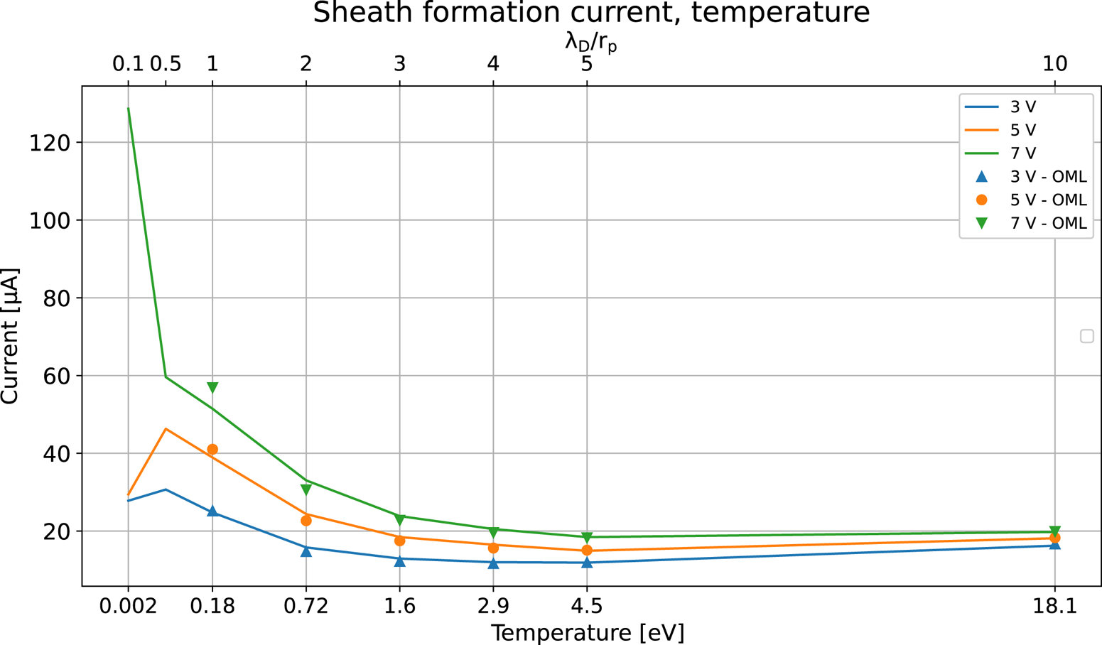The collected current at $100\,\mathrm {\mu }$s was also compared with the OML theory, as seen in figure 3, with a good agreement for simulations where the Debye length exceeds the dimensions of the probe. The sheath formation time was derived from the current at the point where the derivative of the current was equal to zero and the current was within 2 per cent of the average current in the subsequent $2\,\mathrm {\mu }$s. This algorithm seemed to agree well with results from the analysis of the particle distribution that we can see in figure 2. Examples of sheath formation times can be seen in figure 1 for $\lambda _D/r_p = 0.5, 1$ and 5.

Figure 1.

Sheath formation time for $\lambda _D/r_p = 0.5$, 1 and 2 with $T_e$ respectively 0.04525, 0.181 and 18.1 eV. The bias was 5 V and the $n_e=n_i =1.0\times 10^{11}\,{\rm m}^{-3}$. The formation time is taken to be the point where the current has reached a stable level.

Figure 2.

Ion and electron density as a function of the radius normalised to the Debye length. The data are the mean value densities at a given radial distance from the probe along the $x, y$ and $z$ axes in both positive and negative directions. The density is plotted for each of the time stamps shown in the upper figure and categorised respectively into the formation period or the relaxation period. Here, $\lambda _D/r_p = 1$, $T_e = 0.181$ eV, the probe bias was 5 V and the density of the ambient plasma was $n_e=n_i = 1.0\times 10^{11}\,{\rm m}^{-3}$.

Figure 3.

Simulated currents for probe biases at 3, 5 and 7 V for temperatures from 0.0181 to 18.1 eV compared with the currents given by the OML theory. The plasma density was fixed at $1\times 10^{11}\,{\rm m}^{-3}$.

6.1. Temperature dependency

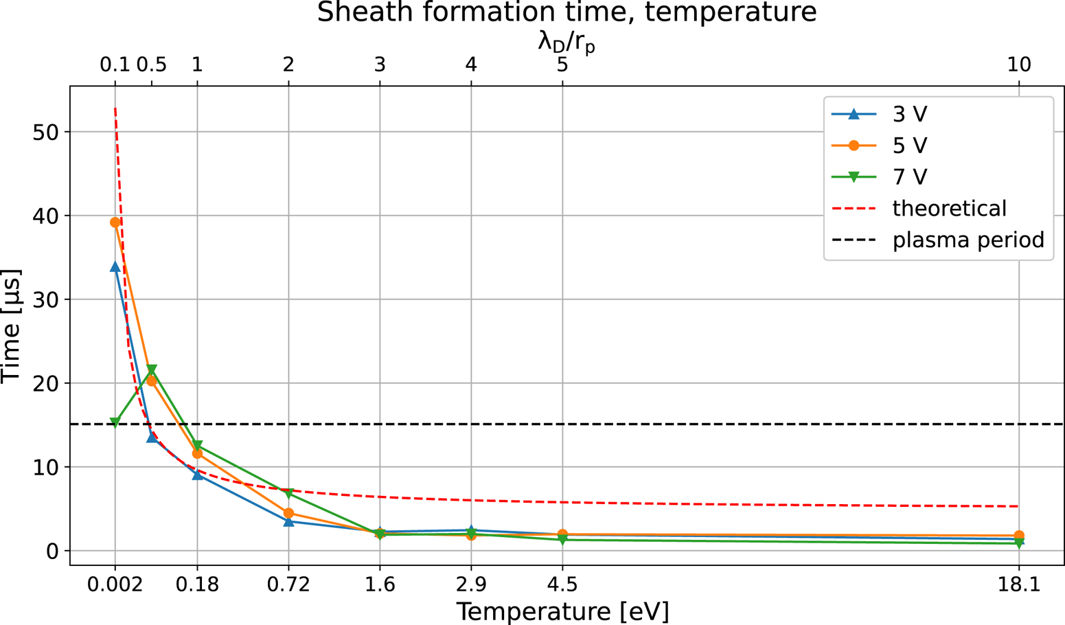
The sheath formation time for plasma temperatures from ranging from 0.0181 to 18.1 eV was simulated for probe biases at 3, 5 and 7 V where the plasma density was fixed at $1\times 10^{11}\,{\rm m}^{-3}$. In figure 4, the extracted sheath formation times are shown as a function of the temperature and the relationship between the corresponding Debye length and the probe radius $\lambda _D/r_p$. For Debye lengths greater than the probe radius, the bias does not have a significant influence on the sheath formation time and for temperatures giving a $\lambda _D/r_p$ relationship larger than 4 the formation time seems to be less affected by the temperature as well.

Figure 4.

Sheath formation times for plasma temperatures from 0.0181 to 18.1 eV and plasma density fixed at $1\times 10^{11}\,{\rm m}^{-3}$. The probe was biased at 3, 5 and 7 V.

In figure 5 we see the particle distribution for Debye length/probe radius from 0.5 to 10 given by temperatures from 0.04525 to 18.1 eV. When the probe is operated in the thin sheath regime, it has a thicker sheath than when it is operated in the thick sheath regime. This can be miss leading. However, we must keep in mind that the Debye length for the $\lambda _D/r_p =0.5$ is 5 mm and the Debye length for the $\lambda _D/r_p =10$ is 100 mm and the sheath size is relative to the Debye length and not the probe radius. In addition, the density variations for the thick sheath are small, and it is difficult to determine the actual sheath size based on these results.

Figure 5.

Particle distribution for Debye length/probe radius from 0.5 to 10 given by temperatures from 0.04525 to 18.1 eV. The plasma density was fixed at $1\times 10^{11}\,{\rm m}^{-3}$ and the probe was biased at 5 V.

We also observe that the sheath goes from a classic monotonic sheath in the thin sheath regime to a non-monotonic in the thick sheath regime where a potential well forms and a fraction of the repelled electrons are returned to the probe (Hobbs & Wesson Reference Hobbs and Wesson1967; Wang et al. Reference Wang, Pilewskie, Hsu and Horányi2016)

6.2. Density dependency

Figure 6 shows the formation time for a probe biased at 5 V with densities ranging from $1.0\times 10^{9}$ to $1.0\times 10^{13}\,{\rm m}^{-3}$, and the temperature fixed at 0.181 eV compared with the same temperature simulations presented in figure 4 at 5 V with temperatures ranging from 0.0181 to 18.1 eV and the density fixed at $1\times 10^{11}\,{\rm m}^{-3}$. Both simulations give the same Debye length vs. probe radius relationship. The theoretical corresponding values, given by (3.5), were compared. We see that using a Debye length as a guiding measure for the formation time is misleading. However, in the thin sheath it makes sense to relate it to the plasma frequency, which is a density dependent quantity, as expressed in (3.1). In figure 7 we see that the sheath size is comparable for the two cases, where the upper curves have a plasma temperature of 18.1 eV and a density of $1.0\times 10^{11}\,{\rm m}^{-3}$ and the lower curves have a plasma temperature of 0.181 eV and a density of $1.0\times 10^{13}\,{\rm m}^{-3}$, both curves having the same Debye lengths.

Figure 6.

Comparison of sheath formation times for the same Debye lengths. The exponential line has varying temperature ranging from 0.00181 to 18.1 eV and a fixed density at $1.0\times 10^{11}\,{\rm m}^{-3}$. The linear curve has a varying density from $1.0\times 10^{9}\,{\rm m}^{-3}$ to $1.0\times 10^{13}$ and fixed the temperature at 0.181 eV. The probe was for all cases biased at 5 V.

Figure 7.

Sheath densities, the same Debye length, where the upper line has a plasma temperature of 18.1 eV and a density of $1.0\times 10^{11}\,{\rm m}^{-3}$, while the lower line has a plasma temperature of 0.181 eV and a density of $1.0\times 10^{13}\,{\rm m}^{-3}$. The probe was for all cases biased at 5 V.

6.3. Mass dependency

Figure 8 shows the formation time as a function of the ion mass, ranging from 1 to 16 amu. The probe was biased at 3, 5 and 7 V, the temperature was 0.181 eV and the density was $1\times 10^{11}\,{\rm m}^{-3}$ giving a Debye length equal to the probe radius. For all probe biases, we find that the simulated result agrees well with Lobbia's approximation, where a quadrupling of the ion mass approximately doubles the time.

Figure 8.

Sheath formation time for ion masses ranging from 1 to 16 amu. The probe was biased at 3, 5 and 7 V, the temperature was 0.181 eV and the density was $1\times 10^{11}\,{\rm m}^{-3}$.

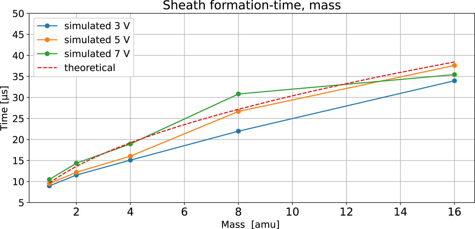
Since the sheath edge is depends on the energy and the energy distribution of the particles, we expect the same distribution of particles, given the same energy and charge of the ions. This is confirmed by figure 9, showing a comparable distribution of ions and electrons in the sheath for hydrogen (1 amu) and oxygen (16 amu) ions. As expected, and according to OML theory and the thin sheath theory, the current is comparable for all ion masses, and we only see small variations at the same order as the noise. From figure 8 we also notice that the formation time is not noticeably affected by the probe bias and that all three probe potentials have comparable formation times.

Figure 9.

Sheath densities compared for ion masses 1 and 16 amu. The probe was biased at 3, 5 and 7 V, the temperature was 0.181 eV and the plasma density was fixed at $1\times 10^{11}\,{\rm m}^{-3}$.