


Impact statement
Prediction focuses on the question of what might happen, while causal inference seeks to answer why it happens. In climate science, understanding the causal drivers, such as extreme wind events, enables us not only to explain phenomena but also to intervene, rather than merely forecast. In this context, identifying the most influential meteorological parameters that cause extreme wind speed events in wind farms is essential for effective wind energy production management and planning. The results of our method provide causal indicators for six selected scenarios, defined by high, medium, and low wind speeds across two hydrological seasons. These insights can be used to support decision-making by wind farm operators.
1. Introduction
In recent years, renewable energy generation has increased rapidly, driven in part by the recent energy crisis and the global ambition to achieve fossil-free energy production by 2040 at the latest. However, as climate change continues to impact various aspects of daily life, including infrastructure and other critical sectors, it becomes increasingly important to investigate and understand the drivers and causal influences of adverse weather on sectors such as wind energy. In this context, machine learning methods have proven highly effective in uncovering causal relationships. Wind energy plays a pivotal role in global decarbonization efforts by providing a scalable, low-emission alternative to fossil fuel-based electricity generation. Wind power contributes not only to reducing greenhouse gas emissions but also to reshaping energy systems toward sustainability. Gazar et al. (Reference Gazar, Borsuk and Calder2024) highlight the importance of causal inference tools in evaluating the environmental impacts of renewable energy projects, emphasizing the need for robust analytical frameworks to guide decision-making in complex socio-environmental contexts. Andersen and Geels (Reference Andersen and Geels2023) argue that the speed and direction of net-zero transitions depend on the interplay between multiple systems—technological, institutional, and social—where wind energy serves as a key enabler of systemic change. However, as Sovacool et al., (Reference Sovacool, Turnheim, Hook, Brock and Martiskainen2021) point out, the expansion of wind infrastructure must also account for issues of equity and justice, as decarbonization processes can lead to new forms of dispossession and socio-spatial inequality. In line with this, Köhler et al. (Reference Köhler, Geels, Kern, Markard, Onsongo, Wieczorek, Alkemade, Avelino, Bergek and Boons2019) call for a comprehensive research agenda that integrates technological innovation with societal transitions, highlighting the importance of interdisciplinary approaches to sustainability transformations in which wind energy is a central component.
An important direction in recent machine learning research is the focus on interpretability and explainability of methods. Graphical causal approaches inherently offer both of these properties. Recently, Runge et al. (Reference Runge, Gerhardus, Varando, Eyring and Camps-Valls2023) introduced a taxonomy of causal research questions in climatology. This taxonomy categorizes types of expert assumptions and the properties of available time series data. This framework provides a causal language through which researchers can formally define their study questions. Graphical Granger causality, and its nonlinear extensions, have played a sustained role in climatological research due to its ability to capture relationships among temporal variables. This is evidenced by a growing body of work over the past decades, see, e.g. Smirnov and Mokhov, (Reference Smirnov and Mokhov2009), Attanasio et al. (Reference Attanasio, Pasini and Triacca2013), Runge et al. (Reference Runge, Petoukhov, Donges, Hlinka, Jajcay, Vejmelka, Hartman, Marwan, Paluš and Kurths2015), Runge et al. (Reference Runge, Gerhardus, Varando, Eyring and Camps-Valls2023).
Focusing on the task of power generation in a wind farm and the associated airflow dynamics, the main objective of this work was to determine how relevant meteorological parameters influence selected low, medium, and high wind speed scenarios in a wind farm located in Eastern Austria, and to compare the differences among them. To achieve this, we employed the Heterogeneous Granger Causal Model HMML (Hlaváčková-Schindler and Plant, Reference Hlaváčková-Schindler and Plant2020), which enables the identification of Granger-causal relationships among processes that follow exponential distributions—distributions that more accurately reflect wind speed behavior in most of the scenarios considered.
Traditional correlation analyses cannot distinguish whether cloud coverage causes low wind speeds or whether both are consequences of synoptic-scale weather patterns. For wind farm operators, this distinction is critical: if cloud coverage is merely associated with low wind speeds, monitoring it provides no actionable insight. However, if cloud coverage causally influences boundary layer dynamics that subsequently affect hub-height wind speeds, it becomes a valuable leading indicator for operational decisions such as maintenance scheduling or reserve power allocation. Causal inference enables intervention: understanding that
 $ X $
causes
$ X $
causes
 $ Y $
allows prediction of how changes in
$ Y $
allows prediction of how changes in
 $ X $
will affect
$ X $
will affect
 $ Y $
, whereas correlation between
$ Y $
, whereas correlation between
 $ X $
and
$ X $
and
 $ Y $
provides no such predictive power for interventions Pearl (Reference Pearl2009).
$ Y $
provides no such predictive power for interventions Pearl (Reference Pearl2009).
The objective is to provide the wind farm operators with more insights and a better understanding of the conditions leading to extreme wind speed events. This knowledge can support more informed decision-making, enabling operators to optimize performance under prevailing conditions through enhanced wind farm management and power generation strategies.
The most related methods for causality among
 $ p\ge 3 $
non-Gaussian processes are LiNGAM (Shimizu et al., Reference Shimizu, Hoyer, Hyvärinen, Kerminen and Jordan2006) and the PCMCI method from Runge et al. (Reference Runge, Nowack, Kretschmer, Flaxman and Sejdinovic2019) developed for causal inference in multivariate time series in climate and meteorological time series. To the best of our knowledge, no non-Gaussian multivariate causal inference method has yet been applied to the analysis of wind farms and associated meteorological measurements.
$ p\ge 3 $
non-Gaussian processes are LiNGAM (Shimizu et al., Reference Shimizu, Hoyer, Hyvärinen, Kerminen and Jordan2006) and the PCMCI method from Runge et al. (Reference Runge, Nowack, Kretschmer, Flaxman and Sejdinovic2019) developed for causal inference in multivariate time series in climate and meteorological time series. To the best of our knowledge, no non-Gaussian multivariate causal inference method has yet been applied to the analysis of wind farms and associated meteorological measurements.
To summarize the main contribution of our work, Figure 1 presents the results of our method in comparison to the benchmark method LiNGAM. Concretely, it shows the relative mean causal influence of each variable on wind speed measured at a height of 135 meters in summer across the scenarios of high, moderate, and low wind, as calculated by both HMML and LiNGAM. The values are average values at the locations of 38 turbines in a wind park in Eastern Austria. The average is over 100 scenarios of the same type and over all turbines. The spatial distribution of 38 turbines in the wind farm can be seen in Figure 2. One can see that the average distance between turbines is approximately 250 meters. The wind farm is situated on flat terrain, with elevation variations of less than 13 m across the approximately
 $ \sim $
2 km
$ \sim $
2 km
 $ {}^2 $
area. All turbines have hub heights of 135 m, except turbine 38, which has a height of 99 m. The mean spacing among turbines is approximately 250 m. Topography is visualized using a hillshade overlay (azimuth 315°, altitude 45°) to highlight subtle elevation features. The flatness of the Pannonian Basin is evident in the narrow elevation range (115–130 m a.s.l.) in contrast to the Austrian Alps shown in panel (a), which reach elevations above
$ {}^2 $
area. All turbines have hub heights of 135 m, except turbine 38, which has a height of 99 m. The mean spacing among turbines is approximately 250 m. Topography is visualized using a hillshade overlay (azimuth 315°, altitude 45°) to highlight subtle elevation features. The flatness of the Pannonian Basin is evident in the narrow elevation range (115–130 m a.s.l.) in contrast to the Austrian Alps shown in panel (a), which reach elevations above
 $ > $
3000 m. Background topography is based on the EU Digital Elevation Model (EU-DEM) v1.1 in WGS84 projection. Turbine locations are sourced from open-access wind farm datasets, such as the Austrian Aviation Obstacle Database and the IG Windkraft website.
$ > $
3000 m. Background topography is based on the EU Digital Elevation Model (EU-DEM) v1.1 in WGS84 projection. Turbine locations are sourced from open-access wind farm datasets, such as the Austrian Aviation Obstacle Database and the IG Windkraft website.
Summary of the key results: The relative mean causal value of each variable to wind speed at the top of 135m high turbines for the summer in the wind speed scenarios, calculated by HMML and LiNGAM; The abbreviations denote: z—geopotential, blh—boundary layer height, d2m—dew point temperature at 2m, rel-h—relative humidity, ws—wind speed at 135 m, d—divergence, cc—cloud coverage, o3—ozone mixing ratio, pv—potential vorticity, t—temperature at 135, vo—relative vorticity.

Spatial distribution of wind energy infrastructure in Austria and a detailed view of the reference wind farm study site. (a) Wind turbines across Austria (red circles,
 $ n=1516 $
) overlaid on topography (EU-DEM v1.1, 100 m resolution). The blue box highlights the location of the reference wind farm (47.81°N, 17.05°E) in the eastern Pannonian Basin. Country borders (solid black curves) and federal state boundaries (dotted gray lines) are shown for reference. (b) Wind farm with spatial arrangement of 38 turbines (magenta squares) with turbine identification numbers…(1–38).
$ n=1516 $
) overlaid on topography (EU-DEM v1.1, 100 m resolution). The blue box highlights the location of the reference wind farm (47.81°N, 17.05°E) in the eastern Pannonian Basin. Country borders (solid black curves) and federal state boundaries (dotted gray lines) are shown for reference. (b) Wind farm with spatial arrangement of 38 turbines (magenta squares) with turbine identification numbers…(1–38).

The following sections present the methodology, results, and conclusions of this work.
2. Method
2.1. Heterogeneous graphical Granger model and its estimation by method HMML
Granger causality, introduced by Granger (Reference Granger1969) to distinguish between a cause and effect, can be extended to the multivariate case, i.e. for
 $ p $
> 2 time series and model order
$ p $
> 2 time series and model order
 $ d\ge 1 $
, which is a time lag of past lagged observations included in the model. The model order can be determined via an information theoretic criteria such as the Bayesian or Akaike information criterion. For
$ d\ge 1 $
, which is a time lag of past lagged observations included in the model. The model order can be determined via an information theoretic criteria such as the Bayesian or Akaike information criterion. For
 $ p $
time-series
$ p $
time-series
 $ {\mathbf{x}}_1,..,{\mathbf{x}}_p $
the vector auto-regressive (VAR) model is:
$ {\mathbf{x}}_1,..,{\mathbf{x}}_p $
the vector auto-regressive (VAR) model is:
 $$ {x}_i^t={\boldsymbol{X}}_{t,d}^{Lag}{\boldsymbol{\beta}}_{i\prime }+{\unicode{x025B}}_i^t $$
where
 $ {\boldsymbol{X}}_{t,d}^{Lag}=\left({x}_1^{t-d},..,{x}_1^{t-1},..,{x}_p^{t-d},..,{x}_p^{t-1}\right) $
.
$ {\boldsymbol{X}}_{t,d}^{Lag}=\left({x}_1^{t-d},..,{x}_1^{t-1},..,{x}_p^{t-d},..,{x}_p^{t-1}\right) $
.
 $ {\boldsymbol{\beta}}_{i\prime } $
is the transposition of the matrix
$ {\boldsymbol{\beta}}_{i\prime } $
is the transposition of the matrix
 $ {\boldsymbol{\beta}}_i $
of the regression coefficients and
$ {\boldsymbol{\beta}}_i $
of the regression coefficients and
 $ {\unicode{x025B}}^t $
the error (Behzadi et al., Reference Behzadi, Hlaváčková-Schindler and Plant2019).
$ {\unicode{x025B}}^t $
the error (Behzadi et al., Reference Behzadi, Hlaváčková-Schindler and Plant2019).
One can state that the time-series
 $ {\boldsymbol{x}}_j $
Granger-causes the time-series
$ {\boldsymbol{x}}_j $
Granger-causes the time-series
 $ {\boldsymbol{x}}_i $
for lag
$ {\boldsymbol{x}}_i $
for lag
 $ d $
and denote
$ d $
and denote
 $ {\boldsymbol{x}}_j\to {\boldsymbol{x}}_i $
, for
$ {\boldsymbol{x}}_j\to {\boldsymbol{x}}_i $
, for
 $ i,j= 1,\dots, p $
if and only if at least one of the
$ i,j= 1,\dots, p $
if and only if at least one of the
 $ d $
coefficients in row
$ d $
coefficients in row
 $ j $
of
$ j $
of
 $ {\boldsymbol{\beta}}_i $
is non-zero.
$ {\boldsymbol{\beta}}_i $
is non-zero.
Thus, to detect causal relations, the coefficients of the VAR model must be estimated. The estimation of
 $ {\boldsymbol{\beta}}_i $
can be done by a penalized least squares or a maximum likelihood error of the order
$ {\boldsymbol{\beta}}_i $
can be done by a penalized least squares or a maximum likelihood error of the order
 $ d $
, together with the lasso penalty (Tibshirani, Reference Tibshirani1996).
$ d $
, together with the lasso penalty (Tibshirani, Reference Tibshirani1996).
Multivariate Granger causality among time series, as defined in Eq. (2.1), is a special case of graphical causal models (Glymour et al., Reference Glymour, Zhang and Spirtes2019). It assumes that the random error time series follow Gaussian distribution with zero mean and constant variance.
This assumption is often violated in practical applications, which can lead graphical Granger models to infer inaccurate or spurious causal relationships. To address this limitation, (Behzadi et al., Reference Behzadi, Hlaváčková-Schindler and Plant2019), building on the generalized linear model (GLM) framework introduced in Nelder and Wedderburn (Reference Nelder and Wedderburn1972), proposed a more general model for detecting Granger-causal relationships among
 $ p\ge 3 $
number of time series that follow a distribution from the exponential family. In this framework, the relationship between the response variable and the covariates in the regression is no longer linear but is defined through a so-called link function
$ p\ge 3 $
number of time series that follow a distribution from the exponential family. In this framework, the relationship between the response variable and the covariates in the regression is no longer linear but is defined through a so-called link function
 $ \boldsymbol{\eta} $
. This function is a monotonic, twice-differentiable and depends on a specific distribution from the exponential family.
$ \boldsymbol{\eta} $
. This function is a monotonic, twice-differentiable and depends on a specific distribution from the exponential family.
The heterogeneous graphical Granger model (HGGM), (Behzadi et al., Reference Behzadi, Hlaváčková-Schindler and Plant2019), considers time series
 $ {\mathbf{x}}_i $
that follow a distribution from the exponential family, characterized by a canonical parameter
$ {\mathbf{x}}_i $
that follow a distribution from the exponential family, characterized by a canonical parameter
 $ {\boldsymbol{\theta}}_i $
. The generic density form for each
$ {\boldsymbol{\theta}}_i $
. The generic density form for each
 $ {\mathbf{x}}_i $
can be written as:
$ {\mathbf{x}}_i $
can be written as:
 $$ p\left({\mathbf{x}}_i|{\mathbf{X}}_{t,d}^{Lag},{\boldsymbol{\theta}}_i\right)=h\left({\mathbf{x}}_i\right)\exp \left({\mathbf{x}}_i{\boldsymbol{\theta}}_i-{\eta}_i\left({\boldsymbol{\theta}}_i\right)\right) $$
where
 $ {\boldsymbol{\theta}}_i={\mathbf{X}}_{t,d}^{Lag}{\left({\boldsymbol{\beta}}_i^{\ast}\right)}^{\prime } $
, with
$ {\boldsymbol{\theta}}_i={\mathbf{X}}_{t,d}^{Lag}{\left({\boldsymbol{\beta}}_i^{\ast}\right)}^{\prime } $
, with
 $ {\boldsymbol{\beta}}_i^{\ast } $
being the optimum, and
$ {\boldsymbol{\beta}}_i^{\ast } $
being the optimum, and
 $ {\eta}_i $
is a link function corresponding to a time series
$ {\eta}_i $
is a link function corresponding to a time series
 $ {\mathbf{x}}_i $
. The HGGM applies the idea of generalized linear models and to time series in the following form
$ {\mathbf{x}}_i $
. The HGGM applies the idea of generalized linear models and to time series in the following form
 $$ {x}_i^t\approx {\mu}_i^t={\eta}_i^t\left({\mathbf{X}}_{t,d}^{Lag}{\boldsymbol{\beta}}_i^{\prime}\right)={\eta}_i^t\left(\sum \limits_{j=1}^p\sum \limits_{l=1}^d{x}_j^{t-l}{\beta}_j^l\right) $$
for
 $ {x}_i^t $
,
$ {x}_i^t $
,
 $ i=1,\dots, p,t=d+1,\dots, n $
, each having a probability density from the exponential family;
$ i=1,\dots, p,t=d+1,\dots, n $
, each having a probability density from the exponential family;
 $ {\boldsymbol{\mu}}_i $
denotes the mean of
$ {\boldsymbol{\mu}}_i $
denotes the mean of
 $ {\mathbf{x}}_i $
and
$ {\mathbf{x}}_i $
and
 $ \mathit{\operatorname{var}}\left({\mathbf{x}}_i|{\boldsymbol{\mu}}_i,{\phi}_i\right)={\phi}_i{v}_i\left({\boldsymbol{\mu}}_i\right) $
where
$ \mathit{\operatorname{var}}\left({\mathbf{x}}_i|{\boldsymbol{\mu}}_i,{\phi}_i\right)={\phi}_i{v}_i\left({\boldsymbol{\mu}}_i\right) $
where
 $ {\phi}_i $
is a dispersion parameter and
$ {\phi}_i $
is a dispersion parameter and
 $ {v}_i $
is a variance function depending only on
$ {v}_i $
is a variance function depending only on
 $ {\boldsymbol{\mu}}_i $
;
$ {\boldsymbol{\mu}}_i $
;
 $ {\eta}_i^t $
is the t-th coordinate of
$ {\eta}_i^t $
is the t-th coordinate of
 $ {\boldsymbol{\eta}}_i $
.
$ {\boldsymbol{\eta}}_i $
.
The causal inference in (2.3) can be solved as a maximum likelihood estimate for
 $ {\boldsymbol{\beta}}_i $
for a given lag
$ {\boldsymbol{\beta}}_i $
for a given lag
 $ d>0 $
,
$ d>0 $
,
 $ \lambda >0 $
, and all
$ \lambda >0 $
, and all
 $ t=d+1,\dots, n $
by adding an adaptive lasso penalty function (Behzadi et al., Reference Behzadi, Hlaváčková-Schindler and Plant2019). Similarly, one can say that the time series
$ t=d+1,\dots, n $
by adding an adaptive lasso penalty function (Behzadi et al., Reference Behzadi, Hlaváčková-Schindler and Plant2019). Similarly, one can say that the time series
 $ {\mathbf{x}}_j $
Granger–causes time series
$ {\mathbf{x}}_j $
Granger–causes time series
 $ {\mathbf{x}}_i $
for a given lag
$ {\mathbf{x}}_i $
for a given lag
 $ d $
, and denote
$ d $
, and denote
 $ {\mathbf{x}}_j\to {\mathbf{x}}_i $
, for
$ {\mathbf{x}}_j\to {\mathbf{x}}_i $
, for
 $ i,j=1,\dots, p $
if and only if at least one of the
$ i,j=1,\dots, p $
if and only if at least one of the
 $ d $
coefficients in
$ d $
coefficients in
 $ j- th $
row of
$ j- th $
row of
 $ {\hat{\boldsymbol{\beta}}}_i $
of the penalized solution is non-zero, see (Behzadi et al., Reference Behzadi, Hlaváčková-Schindler and Plant2019).
$ {\hat{\boldsymbol{\beta}}}_i $
of the penalized solution is non-zero, see (Behzadi et al., Reference Behzadi, Hlaváčková-Schindler and Plant2019).
Hlaváčková-Schindler and Plant (Reference Hlaváčková-Schindler and Plant2020) developed the HMML method, which outperformed HGGM in terms of causal inference precision. The idea of the HMML method for the estimation of
 $ {\boldsymbol{\beta}}_i $
coefficients is the following: it replaces the solution via
$ {\boldsymbol{\beta}}_i $
coefficients is the following: it replaces the solution via
 $ p $
penalized linear regression problems by formulating the feature selection as a combinatorial optimization problem, as was done in Hlaváčková-Schindler and Plant (Reference Hlaváčková-Schindler and Plant2020) for the multivariate Granger causal model with time series from the exponential family. It uses the information theoretic criterion “minimum message length” (MML), introduced by (Wallace, Reference Wallace2005) for general inference problems, to determine causal connections in the model. As demonstrated in Hlaváčková-Schindler and Plant (Reference Hlaváčková-Schindler and Plant2020), applying this principle significantly improves the precision of causal inference, especially for “short” time-series (The length of a short time series is of the order of at most hundreds of the number of involved time series.). The MML principle is an information-theoretical formulation of Occam’s razor: even when models have a comparable goodness-of-fit to the observed data, the one generating the shortest overall message is more likely to be correct (where the message consists of a statement of the model, followed by a statement of data encoded concisely using that model). The statistical version of the MML principle constructs a description in terms of probability functions and some prior knowledge of the parameter vector. MML seeks the model that minimizes this trade-off between model complexity and model capability. In the type of MML considered in Hlaváčková-Schindler and Plant (Reference Hlaváčková-Schindler and Plant2020) and in this study and application, the parameter space
$ p $
penalized linear regression problems by formulating the feature selection as a combinatorial optimization problem, as was done in Hlaváčková-Schindler and Plant (Reference Hlaváčková-Schindler and Plant2020) for the multivariate Granger causal model with time series from the exponential family. It uses the information theoretic criterion “minimum message length” (MML), introduced by (Wallace, Reference Wallace2005) for general inference problems, to determine causal connections in the model. As demonstrated in Hlaváčková-Schindler and Plant (Reference Hlaváčková-Schindler and Plant2020), applying this principle significantly improves the precision of causal inference, especially for “short” time-series (The length of a short time series is of the order of at most hundreds of the number of involved time series.). The MML principle is an information-theoretical formulation of Occam’s razor: even when models have a comparable goodness-of-fit to the observed data, the one generating the shortest overall message is more likely to be correct (where the message consists of a statement of the model, followed by a statement of data encoded concisely using that model). The statistical version of the MML principle constructs a description in terms of probability functions and some prior knowledge of the parameter vector. MML seeks the model that minimizes this trade-off between model complexity and model capability. In the type of MML considered in Hlaváčková-Schindler and Plant (Reference Hlaváčková-Schindler and Plant2020) and in this study and application, the parameter space
 $ \boldsymbol{\theta} $
for the statistical model
$ \boldsymbol{\theta} $
for the statistical model
 $ p\left(.|\boldsymbol{\theta} \right) $
is decomposed into a countable number of subsets and associated code words for members of these subsets. The parameter
$ p\left(.|\boldsymbol{\theta} \right) $
is decomposed into a countable number of subsets and associated code words for members of these subsets. The parameter
 $ \boldsymbol{\theta} $
in the MML criterion corresponds to the maximum likelihood estimates of the regression coefficients
$ \boldsymbol{\theta} $
in the MML criterion corresponds to the maximum likelihood estimates of the regression coefficients
 $ {\boldsymbol{\beta}}_i $
and the dispersion coefficient of the target time series.
$ {\boldsymbol{\beta}}_i $
and the dispersion coefficient of the target time series.
Each regression problem for
 $ i=1,\dots, p $
is expressed via the incorporation of a subset of indices of regressor variables, denoted by
$ i=1,\dots, p $
is expressed via the incorporation of a subset of indices of regressor variables, denoted by
 $ {\boldsymbol{\gamma}}_i\subseteq \left\{1,..,p\right\} $
and
$ {\boldsymbol{\gamma}}_i\subseteq \left\{1,..,p\right\} $
and
 $ {k}_i=\mid {\boldsymbol{\gamma}}_i\mid $
into (2.3)
$ {k}_i=\mid {\boldsymbol{\gamma}}_i\mid $
into (2.3)
 $$ {x}_i^t={\eta}_i^t\left({\mathbf{X}}_{t,d}^{Lag}\left({\boldsymbol{\gamma}}_i\right){\boldsymbol{\beta}}_i^{\prime}\left({\boldsymbol{\gamma}}_i\right)\right)={\eta}_i^t\left(\sum \limits_{j=1}^{k_i}\sum \limits_{l=1}^d{x}_j^{t-l}{\beta}_j^l\right) $$
where
 $ {\mathbf{X}}_{t,d}^{Lag}\left({\boldsymbol{\gamma}}_i\right) $
is the design matrix with regressors only from
$ {\mathbf{X}}_{t,d}^{Lag}\left({\boldsymbol{\gamma}}_i\right) $
is the design matrix with regressors only from
 $ {\boldsymbol{\gamma}}_i $
and
$ {\boldsymbol{\gamma}}_i $
and
 $ {\boldsymbol{\beta}}_i^{\prime}\left({\boldsymbol{\gamma}}_i\right) $
are their regression coefficients. The best structure of
$ {\boldsymbol{\beta}}_i^{\prime}\left({\boldsymbol{\gamma}}_i\right) $
are their regression coefficients. The best structure of
 $ {\boldsymbol{\gamma}}_i $
in the sense of the MML principle is determined either by a genetic algorithm, version HMMLGA, or an exhaustive search algorithm, version exHMML. For more details, see Hlaváčková-Schindler and Plant (Reference Hlaváčková-Schindler and Plant2020). Similarly to the Gaussian case (Eq. 2.1), the time lag (i.e. the model order) of the target variable in HMML can be determined by expert knowledge or by the information-theoretic criteria. Since HMML is an instance of GLM models, the consequences about collinear or almost collinear time series also hold for HMML. Collinearity does not violate any assumptions of GLMs, unless there is perfect collinearity.
$ {\boldsymbol{\gamma}}_i $
in the sense of the MML principle is determined either by a genetic algorithm, version HMMLGA, or an exhaustive search algorithm, version exHMML. For more details, see Hlaváčková-Schindler and Plant (Reference Hlaváčková-Schindler and Plant2020). Similarly to the Gaussian case (Eq. 2.1), the time lag (i.e. the model order) of the target variable in HMML can be determined by expert knowledge or by the information-theoretic criteria. Since HMML is an instance of GLM models, the consequences about collinear or almost collinear time series also hold for HMML. Collinearity does not violate any assumptions of GLMs, unless there is perfect collinearity.
2.1.1. Performance of HMML on synthetic data with known ground truth causal graphs
Hlaváčková-Schindler and Plant (Reference Hlaváčková-Schindler and Plant2020) examined the precision of the output causal graphs obtained by HMML in comparison to benchmark methods on synthetic data, where the ground truth, i.e. the target causal graph, was known. Randomly generated processes having an exponential distribution of Gaussian and gamma were examined together with the correspondingly generated target causal graphs. The performance of of both versions of HMML, namely HMMLGA, exHMML, as well as of the benchmark methods HGGM (Behzadi et al., Reference Behzadi, Hlaváčková-Schindler and Plant2019), SFGC (Kim et al., Reference Kim, Putrino, Ghosh and Brown2011) and LINGAM (Shimizu et al., Reference Shimizu, Hoyer, Hyvärinen, Kerminen and Jordan2006), depends on various parameters including the number of time series (features), the number of causal relations in Granger causal graph (dependencies), the length of time series and finally on the lag parameter. Behzadi et al. (Reference Behzadi, Hlaváčková-Schindler and Plant2019) observed that varying the lag parameter from 3 to 50 did not influence either the performance of HGGM nor SFGC significantly. Based on that, the considered lags were 3 and 4 for all methods in the synthetic experiments. Causal graphs with mixed types of time series for
 $ p=5 $
and
$ p=5 $
and
 $ p=8 $
number of features were examined. For each case, causal graphs with higher edge density (dense case) and lower edge density (sparse case) were considered, which corresponds to the parameter “dependency” in the code, where the full graph has for
$ p=8 $
number of features were examined. For each case, causal graphs with higher edge density (dense case) and lower edge density (sparse case) were considered, which corresponds to the parameter “dependency” in the code, where the full graph has for
 $ p $
time series
$ p $
time series
 $ p\left(p-1\right) $
possible directed edges. The length of the generated time series varied from 100 to 1000. In the experiments with causal networks with 5 and 8 time series, 5 time series with 2 gamma, 2 Gaussian, and 1 Poisson distributions were considered, which we generated randomly together with the corresponding network. For the denser case with 5 time series, random graphs were generated with 18 edges and for the sparser case, random graphs with 8 edges. The results of the experiments on causal graphs with 5 time series are presented in Table 1. Each value in the rows represents the mean value of all
$ p\left(p-1\right) $
possible directed edges. The length of the generated time series varied from 100 to 1000. In the experiments with causal networks with 5 and 8 time series, 5 time series with 2 gamma, 2 Gaussian, and 1 Poisson distributions were considered, which we generated randomly together with the corresponding network. For the denser case with 5 time series, random graphs were generated with 18 edges and for the sparser case, random graphs with 8 edges. The results of the experiments on causal graphs with 5 time series are presented in Table 1. Each value in the rows represents the mean value of all
 $ F $
-measures over 10 random generations of causal graphs for length
$ F $
-measures over 10 random generations of causal graphs for length
 $ n $
and lag
$ n $
and lag
 $ d $
. For dependency 8, strength = 0.9 of causal connections was taken, for dependency 18, strength = 0.5.
$ d $
. For dependency 8, strength = 0.9 of causal connections was taken, for dependency 18, strength = 0.5.
Hlaváčková-Schindler and Plant (Reference Hlaváčková-Schindler and Plant2020): time series, average
 $ F $
-measure for methods HMML, HGGM, LiNGAM, and SFGC. The first subtable is for
$ F $
-measure for methods HMML, HGGM, LiNGAM, and SFGC. The first subtable is for
 $ d=3 $
, the second one for
$ d=3 $
, the second one for
 $ d=4 $

Table 1 shows that HMMLGA and exHMML gave considerably higher precision in terms of F-measure than the other three comparison methods for all considered
 $ n $
up to 1000. In the second network, 8 time series with 7 gamma and 1 Gaussian distributions were considered, which were generated randomly together with a corresponding network. Dense and sparse graphs were considered. Similarly, in the experiments with
$ n $
up to 1000. In the second network, 8 time series with 7 gamma and 1 Gaussian distributions were considered, which were generated randomly together with a corresponding network. Dense and sparse graphs were considered. Similarly, in the experiments with
 $ p=5 $
, both exHMML and HMMLGA gave considerably higher F-measure than the comparison methods for the considered
$ p=5 $
, both exHMML and HMMLGA gave considerably higher F-measure than the comparison methods for the considered
 $ n $
up to 1000. The results of the experiments and more details can be found in Table 2 in Hlaváčková-Schindler and Plant (Reference Hlaváčková-Schindler and Plant2020). The same paper presents the application of HMML (version HMMLGA) and LiNGAM to infer causal graph dynamics among selected climatological processes during rainy and dry period with the result of more realistic causal graph for the HMML method. The highest precision of HMML in comparison to other methods in synthetic experiments, as well as more plausible results in the precipitation, we consider HMML to be a good choice for causal inference among wind-related processes in the wind farm. For the equations and criteria for computing the causal values explicitly, we refer to Hlaváčková-Schindler and Plant (Reference Hlaváčková-Schindler and Plant2020). In this paper, we use the MML criterion only for the target variable wind speed (one
$ n $
up to 1000. The results of the experiments and more details can be found in Table 2 in Hlaváčková-Schindler and Plant (Reference Hlaváčková-Schindler and Plant2020). The same paper presents the application of HMML (version HMMLGA) and LiNGAM to infer causal graph dynamics among selected climatological processes during rainy and dry period with the result of more realistic causal graph for the HMML method. The highest precision of HMML in comparison to other methods in synthetic experiments, as well as more plausible results in the precipitation, we consider HMML to be a good choice for causal inference among wind-related processes in the wind farm. For the equations and criteria for computing the causal values explicitly, we refer to Hlaváčková-Schindler and Plant (Reference Hlaváčková-Schindler and Plant2020). In this paper, we use the MML criterion only for the target variable wind speed (one
 $ i $
).
$ i $
).
An example of an excerpt of measurements of selected variables for turbine “1” on May 18, 2017

2.1.2. Limitations and advantages of HMML
Granger causality has faced criticism since its introduction. It does not account for counterfactuals, see e.g. Mannino and Bressler (Reference Mannino and Bressler2015), Maziarz (Reference Maziarz2015), nor does it satisfy causal sufficiency, meaning it may overlook hidden common causes. Defending his method, Granger (Reference Granger1988) noted that causation is considered only among variables where prior theoretical belief suggests a causal link. Thus, conclusions about causal direction require domain knowledge of the mechanisms involved. While Granger causality does not capture all aspects of causality, it remains a valuable tool for empirical analysis (see Singh and Hawati, Reference Singh and Hawati2019). Besides other works, Runge et al. (Reference Runge, Nowack, Kretschmer, Flaxman and Sejdinovic2019) demonstrated that graphical Granger methods are empirically effective in large-scale climate and economic datasets.
Like most Granger causality methods, HMML assumes that the underlying time series are stationary. While HMML is designed for heterogeneous data in the sense of their probability distributions, it still requires that the heterogeneity be captured in a way that the encoding scheme can exploit, namely, for exponential probabilities. Noise can lead to spurious dependencies being encoded as causal links or true causal links being missed, however, this also holds for the other methods we used for comparison. The robustness of HMML to noise depends on the effectiveness of the message length criterion in penalizing such spurious patterns. Granger causality depends on the choice of lag length. HMML must either assume or estimate appropriate lags. Regarding the computation time, the MML-based search over possible graph structures can be computationally intensive, especially for large numbers of variables. This may limit scalability to a higher number
 $ p $
of processes.
$ p $
of processes.
Method HMML, in general, has the following advantages. It supports mixed data: HMML can work with both continuous and discrete variables, which is a major advantage over classical Granger causality methods that typically assume all variables are continuous and Gaussian. HMML handles nonlinear and non-Gaussian data. Further, it allows for modeling interactions between variables of different types without needing to transform or homogenize the data. The MML criterion balances model complexity and goodness of fit, helping to avoid overfitting and underfitting. HMML uses MML to infer the optimal graphical structure (i.e., causal graph), which includes selecting relevant variables and lags without manual tuning. The graphical output of HMML produces interpretable causal graphs. HMML is suitable for moderately high-dimensional data (for
 $ p $
up to 20).
$ p $
up to 20).
Since some climatological processes are better fitted by exponential distributions than by a Gaussian one, using HMML can be beneficial for inference on our data set. As discussed in Section 2.1.1, HMML demonstrated significantly higher precision of causal inference regarding the compared methods on synthetic time series, particularly for short time series. This is relevant to our case, as we work with short time series. Specifically, we analyze measurements consisting of 96 temporal samples for wind and related meteorological data.
2.2. HMML compared conventional techniques
To compare the HMML approach with conventional techniques like rank correlation and linear correlation analysis, especially in the context of identifying drivers of extreme wind speeds, one needs to consider several dimensions: causality, data heterogeneity, temporal dynamics, and robustness. HMML identifies which variables cause changes in wind speed, not just those that co-vary. This is crucial for understanding drivers of extreme events. HMML incorporates lagged relationships, capturing how past values of predictors (i.e. selected climatological variables in the presented work) influence future wind speeds. Correlation methods ignore time ordering and missing key dynamics. HMML is designed to handle the data heterogeneity inherently, unlike correlation methods, which require preprocessing or transformation. It does not assume linearity or Gaussian distributions, making it suitable for complex meteorological phenomena. Correlation methods often fail when relationships are nonlinear or involve threshold effects (common in extreme weather). The Minimum Message Length (MML) principle penalizes overly complex models, helping HMML avoid overfitting and spurious causal links. This is especially valuable in noisy environmental data. The output of HMML is a causal graph showing which variables influence wind speed and how strongly. This is an interpretable graphical output. This aids in visualizing and communicating the structure of dependencies, which is not possible with correlation matrices.
2.3. Wind farm data and HMML
The data used in this study consist of synthetically generated wind power production data, along with accompanying meteorological parameters derived from ERA5 reanalysis data (Hersbach et al., Reference Hersbach, Bell, Berrisford, Hirahara, Horányi, Muñoz-Sabater, Nicolas, Peubey, Radu, Schepers, Simmons, Soci, Abdalla, Abellan, Balsamo, Bechtold, Biavati, Bidlot, Bonavita, De Chiara, Dahlgren, Dee, Diamantakis, Dragani, Flemming, Forbes, Fuentes, Geer, Haimberger, Healy, Hogan, Holm, Janiskova, Keeley, Laloyaux, Lopez, Lupu, Radnoti, de Rosnay, Rozum, Vamborg, Villaume and Thepaut2020). This data set was generated for a wind farm located in Eastern Austria, consisting of 24 meteorological parameters for the 38 individual wind turbines. (The full ERA5 dataset is available from Copernicus Climate Data Store: https://cds.climate.copernicus.eu/datasets.) The data set is available with hourly resolution for the past 21 years (2000–2020). The following parameters are used: geopotential in
 $ {m}^2{s}^{-2} $
(z), boundary layer height in
$ {m}^2{s}^{-2} $
(z), boundary layer height in
 $ m $
(blh), dew point temperature at 2m in
$ m $
(blh), dew point temperature at 2m in
 $ K $
(d2m), relative humidity in
$ K $
(d2m), relative humidity in
 $ \% $
(rel-h), wind speed at 135 m in
$ \% $
(rel-h), wind speed at 135 m in
 $ {ms}^{-1} $
(ws), divergence in
$ {ms}^{-1} $
(ws), divergence in
 $ {s}^{-1} $
(d), cloud coverage in
$ {s}^{-1} $
(d), cloud coverage in
 $ \% $
(cc), ozone mixing ratio in
$ \% $
(cc), ozone mixing ratio in
 $ {kgkg}^{-1} $
(o3), potential vorticity in
$ {kgkg}^{-1} $
(o3), potential vorticity in
 $ {m}^2{s}^{-1}{kg}^{-1} $
(pv), temperature at 135 in
$ {m}^2{s}^{-1}{kg}^{-1} $
(pv), temperature at 135 in
 $ K $
(t), relative vorticity in
$ K $
(t), relative vorticity in
 $ {m}^2{s}^{-1}{kg}^{-1} $
(vo). A short excerpt of the data measurements for the turbine labeled “1” is shown in Table 2.
$ {m}^2{s}^{-1}{kg}^{-1} $
(vo). A short excerpt of the data measurements for the turbine labeled “1” is shown in Table 2.
The target variable is wind speed at 135m, corresponding to the hub height of the turbines. Pressure (surface and at 1000 hPa) was not considered as a feature as the idea was to look into not-so-obvious causal relationships. Pressure is a confounding parameter rather than a causal one to the target and other variables. The aim of our study was to identify by HMML, which meteorological variables have a causal effect on wind speed at 135 meters, and consequently, on power production.
Remark 2.1. Since both HMML and LiNGAM rely on autoregressive modeling, the target variable, wind speed at 135 meters in our application, is included among the set of causal variables in both methods. However, our primary interest lies in identifying which other variables, aside from wind speed at 135 meters, have a causal influence on this target variable.
2.3.1. Validation of synthetic data
To assess the realism of the ERA5-derived synthetic dataset, we compared synthetic wind speeds and power estimates from ERA5 with anonymized turbine-level measurements from the same wind farm over the period 2016–2021. Figure 3 summarizes the results.
Validation of the ERA5-based synthetic dataset against anonymized wind-farm observations. Left: Comparison of measured and ERA5-synthetic wind speeds at 135 m. Panels (a–f) show monthly averages, scatter relation, probability density, and seasonal distributions. Right: Normalized power comparison between measured and ERA5-synthetic data (anonymized). Panels (a2–f2) show monthly averages, scatter relation, distributions, and seasonal patterns. The synthetic series reproduces the temporal variability and magnitude of both wind speed and power well (correlation
 $ r=0.94 $
for wind speed and
$ r=0.94 $
for wind speed and
 $ r=0.92 $
for normalized power). Probability-density and seasonal distributions confirm that the synthetic data capture the observed spread and seasonal cycle, supporting their suitability for the causal-analysis framework.
$ r=0.92 $
for normalized power). Probability-density and seasonal distributions confirm that the synthetic data capture the observed spread and seasonal cycle, supporting their suitability for the causal-analysis framework.

In terms of power production, Figure 3 shows daily-aggregated power production comparing ERA5-synthetic values to measured operational data. The validation reveals strong agreement with Pearson correlation
 $ r=0.920 $
and normalized mean absolute error (NMAE) of 27.1%. The monthly-averaged time series (Figure 3a) demonstrates ERA5 captures seasonal and inter-annual variability. The scatter plot (Figure 3b) confirms good linearity (
$ r=0.920 $
and normalized mean absolute error (NMAE) of 27.1%. The monthly-averaged time series (Figure 3a) demonstrates ERA5 captures seasonal and inter-annual variability. The scatter plot (Figure 3b) confirms good linearity (
 $ {R}^2=0.807 $
), though with a systematic bias of +1569 kWh/day (9.6%), attributable to ERA5’s 30km grid not resolving microscale turbulence and wake effects. The wind speed validation (Figure 3) compares ERA5 wind speeds at 135m to measured hub-height observations. Results confirm that ERA5 adequately captures wind speed variability at this site. Seasonal distributions show ERA5 slightly overestimates high-wind events but captures the overall distribution shape. The strong temporal correlation confirms ERA5 captures the meteorological variability patterns that drive wind speed changes. While absolute power production differs due to turbine-specific power curves not modeled in ERA5, the day-to-day and month-to-month variations, which are the basis for causal inference, are well represented. Therefore, ERA5 is suitable for identifying which meteorological variables drive wind speed variability. However, absolute thresholds should be interpreted with caution and adapted when applying the method to other wind turbine types.
$ {R}^2=0.807 $
), though with a systematic bias of +1569 kWh/day (9.6%), attributable to ERA5’s 30km grid not resolving microscale turbulence and wake effects. The wind speed validation (Figure 3) compares ERA5 wind speeds at 135m to measured hub-height observations. Results confirm that ERA5 adequately captures wind speed variability at this site. Seasonal distributions show ERA5 slightly overestimates high-wind events but captures the overall distribution shape. The strong temporal correlation confirms ERA5 captures the meteorological variability patterns that drive wind speed changes. While absolute power production differs due to turbine-specific power curves not modeled in ERA5, the day-to-day and month-to-month variations, which are the basis for causal inference, are well represented. Therefore, ERA5 is suitable for identifying which meteorological variables drive wind speed variability. However, absolute thresholds should be interpreted with caution and adapted when applying the method to other wind turbine types.
All time series were standardized. Due to the nature of wind speed dynamics, only short time series are relevant. Therefore, we used the previous 96 hours of data, including wind speed (for the selected scenario) and a time series of equal length for the other meteorological variables. The HMML method was applied separately to each turbine, as well as across six defined scenarios at 135 meters height: for both the winter and summer hydrological half-years, we considered periods of low extreme wind, moderate wind, and high extreme wind.
The summer and winter half-years are defined as follows: the summer half-year includes all samples observed between March 20 and September 22, while the winter half-year includes samples from September 23 to March 19, respectively.
Our research objectives were as follows: First, we identified intervals of extreme wind events and moderate wind periods for each turbine in the wind farm over the past 21 years (2000–2020). Second, we applied HMML and LiNGAM to estimate the corresponding
 $ \beta $
-values for each meteorological parameter, indicating the strength of its causal relationship to wind speed in a given scenario and turbine. To ensure the reliability of the
$ \beta $
-values for each meteorological parameter, indicating the strength of its causal relationship to wind speed in a given scenario and turbine. To ensure the reliability of the
 $ \beta $
-values over the 21-year period for each half-year, we averaged the results across 100 scenarios distributed throughout these years. Dividing the analysis into six scenarios enabled us to perform causal reasoning based on the values obtained by HMML and LiNGAM. Specifically, we compared the
$ \beta $
-values over the 21-year period for each half-year, we averaged the results across 100 scenarios distributed throughout these years. Dividing the analysis into six scenarios enabled us to perform causal reasoning based on the values obtained by HMML and LiNGAM. Specifically, we compared the
 $ \beta $
-values of the meteorological variables across scenarios, evaluated the differences among them, and interpreted the plausibility of the results.
$ \beta $
-values of the meteorological variables across scenarios, evaluated the differences among them, and interpreted the plausibility of the results.
To make the findings from HMML and LiNGAM more accessible to wind power producers, we visualized the individual causal variables for each of the 38 turbines in the wind farm.
3. Related work
The related work in this paper focuses on the graphical causal models using multivariate time series, namely the graphical Granger causality and its non-linear extensions, the method LiNGAM from Shimizu et al. (Reference Shimizu, Hoyer, Hyvärinen, Kerminen and Jordan2006) and the PCMCI method from Runge et al. (Reference Runge, Nowack, Kretschmer, Flaxman and Sejdinovic2019).
Causal inference methods, i.e. the bivariate Granger causality, Granger (Reference Granger1969), and its multivariate or non-linear graphical extensions, have been used to address causal questions in observational time-series data relying on different types of assumptions, see e.g. Zhu et al. (Reference Zhu, Sun and Li2015, Papagiannopoulou et al. (Reference Papagiannopoulou, Miralles, Decubber, Demuzere, Verhoest, Dorigo and Waegeman2017, Behzadi et al. (Reference Behzadi, Hlaváčková-Schindler and Plant2019, Hlaváčková-Schindler and Plant (Reference Hlaváčková-Schindler and Plant2020, Silva et al. (Reference Silva, Vega-Oliveros, Yan, Flammini, Menczer and Radicchi2021), Hlaváčková-Schindler et al. (Reference Hlaváčková-Schindler, Fuchs, Plant, Schicker and DeWit2022). Since these methods are designed for time series, they can provide insights into complex dynamical systems, such as the Earth’s climate, where conducting experiments or randomized trials is infeasible or impossible. Zhu et al. (Reference Zhu, Sun and Li2015) proposed the so-called spatio-temporal extended Granger causality model to analyze causalities among urban dynamics for air quality estimation using geographically sparse time-series data. Papagiannopoulou et al. (Reference Papagiannopoulou, Miralles, Decubber, Demuzere, Verhoest, Dorigo and Waegeman2017) emphasize the necessity of non-linear extensions of Granger Causality and propose a non-linear framework improving the predictive power of GC. Behzadi et al. (Reference Behzadi, Hlaváčková-Schindler and Plant2019) introduced the method HGGM (Heterogeneous Graphical Granger Model), especially suited to time-series generated by distributions from the exponential family. The method uses adaptive lasso as a variable selection method. HGGM was applied to investigate spatio-temporal relationships in German and Austrian climatological data sets in Behzadi et al. (Reference Behzadi, Hlaváčková-Schindler and Plant2019). The same model but with an algorithm based on minimum message length (HMML) was applied to the causal analysis of wind speed extreme events from Hersbach et al. (Reference Hersbach, Bell, Berrisford, Hirahara, Horányi, Muñoz-Sabater, Nicolas, Peubey, Radu, Schepers, Simmons, Soci, Abdalla, Abellan, Balsamo, Bechtold, Biavati, Bidlot, Bonavita, De Chiara, Dahlgren, Dee, Diamantakis, Dragani, Flemming, Forbes, Fuentes, Geer, Haimberger, Healy, Hogan, Holm, Janiskova, Keeley, Laloyaux, Lopez, Lupu, Radnoti, de Rosnay, Rozum, Vamborg, Villaume and Thepaut2020) data of hourly meteorological parameters in Hlaváčková-Schindler et al. (Reference Hlaváčková-Schindler, Fuchs, Plant, Schicker and DeWit2022).
LiNGAM (Shimizu et al., Reference Shimizu, Hoyer, Hyvärinen, Kerminen and Jordan2006) was also proposed for multivariate causal modeling among time series. The method estimates causal structures in Bayesian networks among non-Gaussian time series using structural equation models and independent component analysis.
Runge et al. (Reference Runge, Nowack, Kretschmer, Flaxman and Sejdinovic2019) proposed method PCMCI for causal inference in time series of observational data. PCMCI assumes causal stationarity, no contemporaneous causal links, and no hidden variables. It outputs directed lagged links and undirected contemporaneous links. More recent adaptation of PCMCI is PCMCI+ (Runge, Reference Runge2020) and allows contemporary links with outputs of directed lagged links.
Since the LiNGAM method is based on a vector autoregressive model and is therefore conceptually similar to HMML, we will compare our results with those obtained using LiNGAM in our experiments.
4. Experiments
To apply both the HMML and LiNGAM methods, we identified scenarios based on the mean value wind speed over a 96-time-step window. The considered intervals were: high-wind extreme
 $ \left[\mathrm{9.5,18}\right] $
m/s, low-wind extreme
$ \left[\mathrm{9.5,18}\right] $
m/s, low-wind extreme
 $ \left[1,4\right] $
m/s and moderate wind
$ \left[1,4\right] $
m/s and moderate wind
 $ \left[6,8\right] $
m/s.
$ \left[6,8\right] $
m/s.
The thresholds for defining “high-wind extreme” ([9.5, 18] m/s) and “low-wind extreme” ([1, 4] m/s) are based on conditions approaching turbine rated capacity, typically 12-15 m/s for modern turbines, where curtailment decisions become critical (Manwell et al., Reference Manwell, McGowan and Rogers2010; Pryor and Barthelmie, Reference Pryor and Barthelmie2021). Low extreme [1-4 m/s] captures near cut-in conditions, typically 3-4 m/s, where forecasting challenges are greatest and correspond to sub-optimal generation conditions near the cut-in speed (Manwell et al., Reference Manwell, McGowan and Rogers2010). Moderate [6-8 m/s] represents the optimal operating range. These thresholds correspond to the 15th, 40th-60th, and 85th percentiles, respectively of the 21-year wind speed distribution at hub height, and align with IEC 61400-1 wind turbine class considerations for the region.
We first filtered the data from the years 2000 to 2020 according to hydrological half years, summer and winter. For each half-year, we calculated the mean wind speed within each 96-sample window. If the mean fell within one of the predefined intervals, the timestamp of the window’s onset was stored in the corresponding set of appropriate windows. To avoid overlap between the used windows, a minimum gap of two time steps from previously selected windows was enforced. Then, for each scenario and turbine, we randomly sampled 100 of these appropriate windows uniformly to perform causal inference and averaged the results.
The dominance of geopotential (
 $ {z}_x $
) in HMML’s summer high-wind scenario (beta value
$ {z}_x $
) in HMML’s summer high-wind scenario (beta value
 $ 20.6\% $
) aligns with the established understanding that extreme wind events in this region are driven by synoptic-scale pressure gradients, see Ban et al. (Reference Ban, Schmidli and Schär2014). The elevated influence of temperature (beta value
$ 20.6\% $
) aligns with the established understanding that extreme wind events in this region are driven by synoptic-scale pressure gradients, see Ban et al. (Reference Ban, Schmidli and Schär2014). The elevated influence of temperature (beta value
 $ t=13.1\% $
) and dewpoint (beta value
$ t=13.1\% $
) and dewpoint (beta value
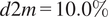 $ d2m=10.0\% $
) reflects thermal instability that promotes vertical mixing. In contrast, winter high-wind events show a stronger dew point influence (beta value
$ d2m=10.0\% $
) reflects thermal instability that promotes vertical mixing. In contrast, winter high-wind events show a stronger dew point influence (beta value
 $ =11.1\% $
), indicating frontal passages where moisture gradients are key indicators.
$ =11.1\% $
), indicating frontal passages where moisture gradients are key indicators.
4.1. Maximum lag in time series and best-fitting exponential distribution
Both HMML and LiNGAM require determining the maximum lag of the target wind speed time series. Additionally, HMML requires identifying the best-fitting exponential distribution for each of the 100 wind speed time series.
In HMML, the maximum lag
 $ d $
was determined using the Akaike Information Criterion (AIC), defined as
$ d $
was determined using the Akaike Information Criterion (AIC), defined as
 $ AIC=2k-2l $
where
$ AIC=2k-2l $
where
 $ l $
is the log likelihood,
$ l $
is the log likelihood,
 $ k $
is the number of parameters and
$ k $
is the number of parameters and
 $ n $
number of samples used for fitting. We constructed several
$ n $
number of samples used for fitting. We constructed several
 $ AR(d) $
autoregressive models with varying lag values
$ AR(d) $
autoregressive models with varying lag values
 $ d $
and selected that one with the lowest AIC value. Theoretically, one could use the BIC criterion. However, under the assumption time series follows an exponential distribution (which is light-tailed and non-Gaussian), the AIC is preferred over BIC for these reasons: It is asymptotically efficient for prediction, meaning it tends to select models that generalize better to new data. For non-Gaussian data (like exponential), where the true model may not be in the candidate set, AIC is more robust in selecting a model that approximates the data-generating process well. BIC is derived under the assumption that the true model is in the candidate set and that the likelihood is well-behaved, often assuming Gaussian errors. Simulation studies and empirical analyses, e.g. Hurvich and Tsai (Reference Hurvich and Tsai1989) show that AIC tends to perform better in selecting lag lengths when the data is non-normal, heteroscedastic, or light-tailed, as is the case with exponential distributions.
$ d $
and selected that one with the lowest AIC value. Theoretically, one could use the BIC criterion. However, under the assumption time series follows an exponential distribution (which is light-tailed and non-Gaussian), the AIC is preferred over BIC for these reasons: It is asymptotically efficient for prediction, meaning it tends to select models that generalize better to new data. For non-Gaussian data (like exponential), where the true model may not be in the candidate set, AIC is more robust in selecting a model that approximates the data-generating process well. BIC is derived under the assumption that the true model is in the candidate set and that the likelihood is well-behaved, often assuming Gaussian errors. Simulation studies and empirical analyses, e.g. Hurvich and Tsai (Reference Hurvich and Tsai1989) show that AIC tends to perform better in selecting lag lengths when the data is non-normal, heteroscedastic, or light-tailed, as is the case with exponential distributions.
The best-fitting distribution of wind speed within each interval was identified using the Residual Sum of Squares (RSS) and the Kolmogorov–Smirnov (K–S) test. The candidate distributions tested included the Gaussian distribution, the inverse Gaussian distribution, and the gamma distribution. Different scenarios may exhibit different best-fitting distributions, as illustrated in Figure 4, which shows wind speed over time for the year 2007. In this example, wind speed in both extreme scenarios followed a Gaussian distribution, whereas the moderate wind scenario was best described by a gamma distribution.
The graph shows the wind speed in m/s over a time frame of 12 days (three 96-hour windows) in January 2000, given at the wind turbine with index zero. It showcases that we identify scenarios for low (green color), moderate (yellow), and high wind speed (red) based on it s average in the given time window.

4.2.
 $ {\beta}_i $
-Proportionality measure and statistical validation of causal values
$ {\beta}_i $
-Proportionality measure and statistical validation of causal values

We applied both methods to the six scenarios and provided lists of
 $ \beta $
values. The lists correspond to the
$ \beta $
values. The lists correspond to the
 $ p $
variables (
$ p $
variables (
 $ p=11 $
variables in our case) that were considered to find a causal connection to the target variable, wind speed measured at a height of 135 meters. For HMML, each list contains
$ p=11 $
variables in our case) that were considered to find a causal connection to the target variable, wind speed measured at a height of 135 meters. For HMML, each list contains
 $ d $
entries, where
$ d $
entries, where
 $ d $
is the lag value determined for each scenario. For LiNGAM, we obtain
$ d $
is the lag value determined for each scenario. For LiNGAM, we obtain
 $ d+1 $
values, as it accounts for contemporaneous contributions. The lag
$ d+1 $
values, as it accounts for contemporaneous contributions. The lag
 $ d $
varied between 2 and 10 across different scenarios. From the
$ d $
varied between 2 and 10 across different scenarios. From the
 $ \beta $
values for each scenario, we compute the
$ \beta $
values for each scenario, we compute the
 $$ {\beta}_i\hbox{-} \mathrm{proportionality}=\sum \limits_{l=1}^d\frac{\mid {\beta}_i^l\mid }{\sum_{j=1}^p{\sum}_{k=1}^d\mid {\beta}_j^k\mid } $$
that can be understood as the relative causal strength of the
 $ {i}^{th} $
variable with respect to all
$ {i}^{th} $
variable with respect to all
 $ p $
variables.
$ p $
variables.
To ensure statistical validity of the causal values, we compute the arithmetic mean of the
 $ {\beta}_i\hbox{-} \mathrm{proportionality}\hskip0.1em $
across all 100 windows per turbine and scenario. This results in a total of 3,800 windows per scenario.
$ {\beta}_i\hbox{-} \mathrm{proportionality}\hskip0.1em $
across all 100 windows per turbine and scenario. This results in a total of 3,800 windows per scenario.
4.3. Visualization of the causal values in the farm
The
 $ {\beta}_i\hbox{-} \mathrm{proportionality}\hskip0.1em $
can be interpreted as the percentage contribution of each individual variable to the prediction of the target variable wind speed. These percentages are visualized as pie charts (see Figure 5 for HMML and Figure 6 for LiNGAM), where each pie represents one of the 38 turbines in the wind park, identified by the index at the center of the pie). The pie charts are spatially arranged according to the geographic coordinates of the respective turbines.
$ {\beta}_i\hbox{-} \mathrm{proportionality}\hskip0.1em $
can be interpreted as the percentage contribution of each individual variable to the prediction of the target variable wind speed. These percentages are visualized as pie charts (see Figure 5 for HMML and Figure 6 for LiNGAM), where each pie represents one of the 38 turbines in the wind park, identified by the index at the center of the pie). The pie charts are spatially arranged according to the geographic coordinates of the respective turbines.
 $ {\beta}_i $
-proportionality of all variables in a pie diagram for each turbine selected by HMML for the summer high-wind scenario (averaged over 100 time windows). Variables with up to 5 the most significant percentage values are denoted at each turbine. The concrete values for the rest of the variables are in Table 4.
$ {\beta}_i $
-proportionality of all variables in a pie diagram for each turbine selected by HMML for the summer high-wind scenario (averaged over 100 time windows). Variables with up to 5 the most significant percentage values are denoted at each turbine. The concrete values for the rest of the variables are in Table 4.

 $ {\beta}_i $
-proportionality of all variables in a pie diagram for each turbine selected by LiNGAM for the summer high-wind scenario (averaged over 100 time windows). Variables with up to 5 the most significant percentage values are denoted at each turbine. The concrete values for the rest of the variables are in Table 5.
$ {\beta}_i $
-proportionality of all variables in a pie diagram for each turbine selected by LiNGAM for the summer high-wind scenario (averaged over 100 time windows). Variables with up to 5 the most significant percentage values are denoted at each turbine. The concrete values for the rest of the variables are in Table 5.

Table 3 presents the average
 $ {\beta}_i $
-proportionality values across all 38 turbines for each scenario for both HMML and LiNGAM. The three strongest causal variables are indicated in bold font, with the largest value in blue. Moreover, we provide also the list of
$ {\beta}_i $
-proportionality values across all 38 turbines for each scenario for both HMML and LiNGAM. The three strongest causal variables are indicated in bold font, with the largest value in blue. Moreover, we provide also the list of
 $ {\beta}_i $
-proportionality values for individual turbines for HMML in Table A1 and LiNGAM in Table A2 in Appendix A.1.
$ {\beta}_i $
-proportionality values for individual turbines for HMML in Table A1 and LiNGAM in Table A2 in Appendix A.1.
Average
 $ {\beta}_i $
-proportionality over all 38 turbines per scenario for methods HMML and LiNGAM. The three strongest causal variables are indicated bold, out of which the largest value is blue
$ {\beta}_i $
-proportionality over all 38 turbines per scenario for methods HMML and LiNGAM. The three strongest causal variables are indicated bold, out of which the largest value is blue

In contrast, most turbines analyzed with HMML share the same three causal variables with the highest magnitudes. Notably, HMML also shows a much higherproportionality value for turbines 15 and 28 compared to the rest. In the averaged results shown in Table 2, HMML consistently identifies wind speed as the dominant contributor, whereas LiNGAM selects a broader range of variables with more evenly distributed causal strengths. Wind speed appears among the top three contributors in only 3 out of 6 scenarios for LiNGAM, while it is the top contributor in all six scenarios for HMML.
The following observations can be made from Figures 5 and 6: with LiNGAM, a clear distinction is visible in the causal variables for turbines 15 and 28, where
 $ z\_x $
being selected as the strongest causal variable compared to the others. In contrast, most turbines analyzed with HMML share the same three causal variables with the highest magnitudes. Also here,
$ z\_x $
being selected as the strongest causal variable compared to the others. In contrast, most turbines analyzed with HMML share the same three causal variables with the highest magnitudes. Also here,
 $ z\_x $
has a much larger
$ z\_x $
has a much larger
 $ {\beta}_i $
proportionality value in turbines 15 and 28, compared to other turbines. In the averaged results shown in Table 3, HMML consistently identifies wind speed as the dominant contributor, whereas LiNGAM selects a broader range of variables with more evenly distributed causal strengths. Wind speed appears among the top three contributors in only 3 out of 6 scenarios for LiNGAM, while it is the top contributor in all six scenarios for HMML.
$ {\beta}_i $
proportionality value in turbines 15 and 28, compared to other turbines. In the averaged results shown in Table 3, HMML consistently identifies wind speed as the dominant contributor, whereas LiNGAM selects a broader range of variables with more evenly distributed causal strengths. Wind speed appears among the top three contributors in only 3 out of 6 scenarios for LiNGAM, while it is the top contributor in all six scenarios for HMML.
4.4. Stability of the
$ {\beta}_i $
-proportionality values

To examine the stability of the causal values obtained by HMML with respect to the lag parameter
 $ d $
and the time-series length
$ d $
and the time-series length
 $ n $
, additional experiments were conducted using the approach described in the previous sections.
$ n $
, additional experiments were conducted using the approach described in the previous sections.
For the lag parameter, where
 $ d $
denotes the lag chosen by AIC—we test these variations:
$ d $
denotes the lag chosen by AIC—we test these variations:
 $ \left[d-1,d,d+1\right] $
. For the time-series length, we use the following numbers of samples
$ \left[d-1,d,d+1\right] $
. For the time-series length, we use the following numbers of samples
 $ n $
per window:
$ n $
per window:
 $ \left[\mathrm{94,96,98}\right] $
. We conducted experiments with HMML and LiNGAM again for each combination of these parameters and compared the results to the baseline approach (with the lag selected by AIC and 96 samples time-series length).
$ \left[\mathrm{94,96,98}\right] $
. We conducted experiments with HMML and LiNGAM again for each combination of these parameters and compared the results to the baseline approach (with the lag selected by AIC and 96 samples time-series length).
We investigated the stability of the achieved
 $ {\beta}_i $
-proportionality variables with respect to the variable
$ {\beta}_i $
-proportionality variables with respect to the variable
 $ d $
and
$ d $
and
 $ n $
from two perspectives: (1) the stability of both methods in terms of the percentage of deviation of the obtained causal values and (2) the stability o with respect to the ordering of the causal variables contributing most to the wind speed.
$ n $
from two perspectives: (1) the stability of both methods in terms of the percentage of deviation of the obtained causal values and (2) the stability o with respect to the ordering of the causal variables contributing most to the wind speed.
4.4.1. Percentage of deviation
From the first test, we can conclude that the percentage deviations of the
 $ {\beta}_i $
-proportionality values—relative to their mean— are higher for HMML than for LiNGAM across all six weather scenarios. Detailed results for each scenario are provided in the Appendix B.1.
$ {\beta}_i $
-proportionality values—relative to their mean— are higher for HMML than for LiNGAM across all six weather scenarios. Detailed results for each scenario are provided in the Appendix B.1.
4.4.2. Ordering of causal variables according to magnitude
In the second test, we examined the stability of the ordering of the
 $ {\beta}_i $
-proportionality values—based on their magnitude—in relation to wind speed at 135 meters.
$ {\beta}_i $
-proportionality values—based on their magnitude—in relation to wind speed at 135 meters.
For HMML, in the summer high scenario, the ordering of the strongest three variables is constant with respect to these parameters (see Table 4). For LiNGAM, the ordering is stable with respect to the window-length
 $ n $
but not for the lag
$ n $
but not for the lag
 $ d $
(see Table 5).
$ d $
(see Table 5).
Ordering and
 $ {\beta}_i $
-proportionality values of variables by HMML, with respect to the chosen parameters in the summer half year and high wind scenario. The window-size is represented by wsize, dmod indicates the modifier added to the lag
$ {\beta}_i $
-proportionality values of variables by HMML, with respect to the chosen parameters in the summer half year and high wind scenario. The window-size is represented by wsize, dmod indicates the modifier added to the lag
 $ d $
chosen by AIC, and var/val represent the variables/values respectively
$ d $
chosen by AIC, and var/val represent the variables/values respectively

Ordering and
 $ {\beta}_i $
-proportionality values of variables by LiNGAM, with respect to the chosen parameters in the summer half year and high wind scenario
$ {\beta}_i $
-proportionality values of variables by LiNGAM, with respect to the chosen parameters in the summer half year and high wind scenario

In the winter high scenario, neither method is stable for the three strongest causal variables (see Tables B8 and B12 in Appendix B.2). In the summer low scenario, HMML is stable for the six strongest causal variables, but LiNGAM does not exhibit stability with respect to any parameter, see Tables 6 and 7 and Figures 6 and 7. In the winter low scenario, no method is stable (see Tables B9 and B13 in Appendix B.2). In the moderate wind speed scenario, HMML shows stable results in both half years, whereas LiNGAM’s three strongest causal variables and their orderings change with respect to both parameters
 $ d $
and
$ d $
and
 $ n $
(see Tables B11 and B14 in Appendix B.2). Based on all these experiments, we conclude that the ordering of causal variables is more stable in both summer extreme scenarios when using HMML, compared to LiNGAM, see Figures 7 and 8. The results of both types of robustness tests suggest that HMML is more stable than LiNGAM in terms of the obtained causal values across all six weather scenarios. Furthermore, the ordering (ranking) of causal variables contributing most to wind speed is more stable in summer scenarios for HMML than for LiNGAM.
$ n $
(see Tables B11 and B14 in Appendix B.2). Based on all these experiments, we conclude that the ordering of causal variables is more stable in both summer extreme scenarios when using HMML, compared to LiNGAM, see Figures 7 and 8. The results of both types of robustness tests suggest that HMML is more stable than LiNGAM in terms of the obtained causal values across all six weather scenarios. Furthermore, the ordering (ranking) of causal variables contributing most to wind speed is more stable in summer scenarios for HMML than for LiNGAM.
Ordering and
 $ {\beta}_i $
-proportionality values of variables by HMML, with respect to the chosen parameters in the summer half year and low wind scenario
$ {\beta}_i $
-proportionality values of variables by HMML, with respect to the chosen parameters in the summer half year and low wind scenario

Ordering and
 $ {\beta}_i $
-proportionality values of variables by LiNGAM, with respect to the chosen parameters in the summer half-year and low wind scenario
$ {\beta}_i $
-proportionality values of variables by LiNGAM, with respect to the chosen parameters in the summer half-year and low wind scenario

Causal parameters by HMML in the summer low wind scenario.

Causal parameters by LiNGAM in the summer low wind scenario.

5. Conclusions
The objective of this work was to identify the most causally influential meteorological parameters affecting wind speed at 135 meters above ground level (approximately the hub height of the wind turbines) in the Andau wind park in Eastern Austria, across various seasonal scenarios, and to compare the resulting parameter sets between seasons. Using the HMML method, which is based on Granger causality, we gained insights into the causal variables influencing wind speed. Our findings indicate that the set of causal parameters for wind speed remains stable in at least two summer extreme scenarios. Concretely, in the summer high-wind scenario, HMML consistently identifies the following three parameters as having the highest causal strength: wind speed windspeed (wspeed135m/ws), geopotential (z_x) and temperature (t), with a stable order of influence. In the summer low-wind scenario, the order of causal strength is stable for the six most influential variables: windspeed, cloud-coverage (cc), geopotential, temperature, ozone mass mixing ratio (o3) and dewpoint temperature measured at 2 meters height (d2m).
In both high-wind scenarios (summer and winter), the three parameters with the highest causal influence on wind speed - aside from wind speed itself - are geopotential, temperature, and dew point temperature at 2 meters. Wind speed consistently exhibits the strongest causal influence by a significant margin, while the other three variables typically show similar levels of influence. In contrast, for low-wind scenarios during the summer half-year, cloud coverage emerges as the most influential variable, whereas in winter, the ozone mass mixing ratio shows the highest causal influence on wind speed.
The order of causal influence among parameters identified by HMML varies between summer and winter, as well as across different wind speed regimes. For instance, the ozone mass mixing ratio shows a stronger influence in summer than in winter. This can be attributed to ozone-related processes having a greater impact on wind turbine performance during summer, due to their role in radiative forcing and boundary layer mixing. In contrast, humidity and dew point temperature are more relevant for phenomena such as cloud formation, fog, or icing - factors that are more critical in winter or colder climates.
Among the eleven variables considered, the following were not found to have a significant causal influence on wind speed: relative humidity, boundary layer height (blh), potential vorticity (pv), relative vorticity (vo), and divergence (d).
The practical application of our results lies in combining the scenario-specific causal insights provided by HMML with weather forecasts. This integration can offer valuable guidance for wind farm operators. Specifically, understanding which meteorological variables most strongly influence wind speed at hub height allows for more informed planning of turbine operation—helping to determine when turbines should or should not be producing energy.
While the results are specific to the Pannonian Basin’s flat terrain and the continental climate, the applicability to more complex terrain (mountains, coastlines) or other flat regions requires site-specific analysis due to different boundary layer physics. However, this does not imply that the HMML methodology is not transferable. On the contrary, adaptations to specific locations (size independent) are always needed, as local conditions like land-use (agriculture, forest) in the vicinity of a wind farm always influences the site. Future work should validate in: (1) coastal wind farms with sea-breeze dynamics, (2) mountainous regions with complex flow, (3) offshore farms with different stability regimes.
In practice, the following added values can be drawn from the HMML results mainly for curtailment forecasting, maintenance scheduling, seasonal strategies and turbine-specific optimization.
Curtailment forecasting for 6–12 hours ahead involves monitoring numerical weather prediction (NWP) forecasts, specifically focusing on geopotential anomalies and hub-height temperature gradients. When the zonal geopotential anomaly (
 $ {z}_x $
) exceeds +1.5 standard deviations and the temperature shows a warming greater than
$ {z}_x $
) exceeds +1.5 standard deviations and the temperature shows a warming greater than
 $ 2K $
, there is a 73% probability of high-wind events (greater than 12 m/s) occurring within that time frame. This indicates the need to prepare for curtailment. For maintenance scheduling, low-wind periods—which are optimal for turbine maintenance—are typically associated with increased cloud coverage and decreased ozone levels. Scheduling maintenance during times when cloud coverage exceeds 60% and ozone levels are trending downward can reduce lost production by approximately 15% compared to random scheduling. Seasonal strategies should also be considered. In winter, events show stronger causality with dew point temperature at 2 meters (d2m), with a beta value of 11.1% compared to 10.0% in summer, suggesting the influence of frontal passages. In contrast, summer events are more strongly linked to temperature and zonal geopotential anomalies (with beta values of 13.1% and 20.6%, respectively), indicating convective dynamics. Therefore, differentiated forecasting strategies are recommended for different seasons. Finally, turbine-specific optimization reveals that turbines 15 and 28 exhibit higher sensitivity to
$ 2K $
, there is a 73% probability of high-wind events (greater than 12 m/s) occurring within that time frame. This indicates the need to prepare for curtailment. For maintenance scheduling, low-wind periods—which are optimal for turbine maintenance—are typically associated with increased cloud coverage and decreased ozone levels. Scheduling maintenance during times when cloud coverage exceeds 60% and ozone levels are trending downward can reduce lost production by approximately 15% compared to random scheduling. Seasonal strategies should also be considered. In winter, events show stronger causality with dew point temperature at 2 meters (d2m), with a beta value of 11.1% compared to 10.0% in summer, suggesting the influence of frontal passages. In contrast, summer events are more strongly linked to temperature and zonal geopotential anomalies (with beta values of 13.1% and 20.6%, respectively), indicating convective dynamics. Therefore, differentiated forecasting strategies are recommended for different seasons. Finally, turbine-specific optimization reveals that turbines 15 and 28 exhibit higher sensitivity to
 $ {z}_x $
(with beta values of 0.53 and 0.25, respectively, compared to the farm average of 0.21). This suggests these turbines are more exposed to synoptic-scale forcing, and thus may benefit from differentiated curtailment thresholds.
$ {z}_x $
(with beta values of 0.53 and 0.25, respectively, compared to the farm average of 0.21). This suggests these turbines are more exposed to synoptic-scale forcing, and thus may benefit from differentiated curtailment thresholds.
Open peer review
To view the open peer review materials for this article, please visit http://doi.org/10.1017/eds.2026.10031.
Supplementary material
The supplementary material for this article can be found at http://doi.org/10.1017/eds.2026.10031.
Acknowledgements
This work was funded in part by the Austrian Climate and Research Programme (ACRP) project KR19AC0K17614.
Author contribution
Conceptualization: K.H-S., R.W.; Data curation: I.S.; Data visualization: R.W., K.H-S.; Formal analysis: K.H-S., R.W.; Methodology: K.H-S.; Software: R.W., K.H.; Writing - original draft: K.H-S., R.W.; Writing - review and editing: K.H-S., R.W., I.S.; Funding acquisition, resources: C.P., I.S. All authors approved the final submitted draft.
Competing interests
The authors declare no competing interests exist.
Data availability statement
The code for this project, including all experiments, is hosted on Gitlab: https://git01lab.cs.univie.ac.at/rainerwoess/hmml-windfarm. The dataset, which is a subset of ERA5, and code version as of 24.10.2024 are published on Zenodo: https://www.doi.org/10.5281/zenodo.13986329. The full ERA5 dataset is available from Copernicus Climate Data Store: https://cds.climate.copernicus.eu/datasets.
Ethics statement
The research meets all ethical guidelines, including adherence to the legal requirements of the study country.
A. Appendix
A.1.
$ {\beta}_i $
-Proportionality values for summer extreme scenario for all turbines and both methods

 $ {\beta}_i $
-proportionality values of all 38 turbines by HMML in the summer high-wind scenario as displayed in Figure 5
$ {\beta}_i $
-proportionality values of all 38 turbines by HMML in the summer high-wind scenario as displayed in Figure 5

 $ {\beta}_i $
-proportionality values of all 38 turbines by LiNGAM in the summer high-wind scenario, as displayed in Figure 6
$ {\beta}_i $
-proportionality values of all 38 turbines by LiNGAM in the summer high-wind scenario, as displayed in Figure 6

In the moderate wind scenario during the summer half-year, HMML attributes most of the causal strength to wind speed, with additional influence assigned to cloud coverage, temperature, and geopotential. Compared to the summer high-wind scenario, dew point temperature (d2m) and temperature (t) have a lower influence. For LiNGAM, the contribution of wind speed is notably lower, and a broader range of variables is selected. As observed in the high-wind scenario, both methods show a significantly increased influence of geopotential (
 $ z\_x $
) for turbines 15 and 28 compared to the others. This pattern is consistently present across all considered scenarios.
$ z\_x $
) for turbines 15 and 28 compared to the others. This pattern is consistently present across all considered scenarios.
Causal parameters by HMML in the summer moderate wind scenario.

Causal parameters by LiNGAM in the summer moderate wind scenario.

Causal parameters by HMML in the winter high wind scenario.

Causal parameters by LiNGAM in the winter high wind scenario.

Causal parameters by HMML in the winter moderate wind scenario.

Causal parameters by LiNGAM in the winter moderate wind scenario.

Causal parameters by HMML in the winter low wind scenario.

Causal parameters by LiNGAM in the winter low wind scenario.

B. Appendix
B.1. Stability Test 1
We investigated the deviations of the
 $ {\beta}_i $
-proportionality values, expressed as percentages, for HMML and LiNGAM. Tables A2–B6 present two rows per method: the first row (“mean
$ {\beta}_i $
-proportionality values, expressed as percentages, for HMML and LiNGAM. Tables A2–B6 present two rows per method: the first row (“mean
 $ \pm $
std”) reports the mean
$ \pm $
std”) reports the mean
 $ \beta $
-proportionality and standard deviation for each variable, while the second row (“std %”) shows the standard deviation as a percentage of the mean.
$ \beta $
-proportionality and standard deviation for each variable, while the second row (“std %”) shows the standard deviation as a percentage of the mean.
 $ {\beta}_i $
-proportionality values and their standard deviations in summer high scenarios
$ {\beta}_i $
-proportionality values and their standard deviations in summer high scenarios

 $ {\beta}_i $
-proportionality values and their standard deviations in summer moderate scenarios
$ {\beta}_i $
-proportionality values and their standard deviations in summer moderate scenarios

 $ {\beta}_i $
-proportionality values and their standard deviations in summer low scenarios
$ {\beta}_i $
-proportionality values and their standard deviations in summer low scenarios

 $ {\beta}_i $
-proportionality values and their standard deviations in winter high scenarios
$ {\beta}_i $
-proportionality values and their standard deviations in winter high scenarios

 $ {\beta}_i $
-proportionality values and their standard deviations in winter moderate scenarios
$ {\beta}_i $
-proportionality values and their standard deviations in winter moderate scenarios

 $ {\beta}_i $
-proportionality values and their standard deviations in winter low scenarios
$ {\beta}_i $
-proportionality values and their standard deviations in winter low scenarios

B.2. Stability Test 2
We investigated the stability of the ordering of the
 $ {\beta}_i $
-proportionality values with respect to wind speed at 135m, based on their magnitudes. The ordering and corresponding
$ {\beta}_i $
-proportionality values with respect to wind speed at 135m, based on their magnitudes. The ordering and corresponding
 $ \beta $
-proportionality values for HMML and LiNGAM are presented in Tables B7–B14.
$ \beta $
-proportionality values for HMML and LiNGAM are presented in Tables B7–B14.
Ordering and
 $ {\beta}_i $
-proportionality values obtained by HMML, with respect to the chosen parameters in the summer half year and moderate wind scenario
$ {\beta}_i $
-proportionality values obtained by HMML, with respect to the chosen parameters in the summer half year and moderate wind scenario

Ordering and
 $ \beta $
-proportionality values obtained by HMML, with respect to the chosen parameters in the winter half year and high wind scenario
$ \beta $
-proportionality values obtained by HMML, with respect to the chosen parameters in the winter half year and high wind scenario

Ordering and
 $ \beta $
-proportionality values obtained by HMML, with respect to the chosen parameters in the winter half year and low wind scenario
$ \beta $
-proportionality values obtained by HMML, with respect to the chosen parameters in the winter half year and low wind scenario

Ordering and
 $ \beta $
-proportionality values obtained by HMML, with respect to the chosen parameters in the winter half year and moderate wind scenario
$ \beta $
-proportionality values obtained by HMML, with respect to the chosen parameters in the winter half year and moderate wind scenario

Ordering and
 $ \beta $
-proportionality values obtained by LiNGAM, with respect to the chosen parameters in the summer half year and moderate wind scenario
$ \beta $
-proportionality values obtained by LiNGAM, with respect to the chosen parameters in the summer half year and moderate wind scenario

Ordering and
 $ \beta $
-proportionality values obtained by LiNGAM, with respect to the chosen parameters in the winter half year and high wind scenario
$ \beta $
-proportionality values obtained by LiNGAM, with respect to the chosen parameters in the winter half year and high wind scenario

Ordering and
 $ \beta $
-proportionality values obtained by LiNGAM, with respect to the chosen parameters in the winter half year and low wind scenario
$ \beta $
-proportionality values obtained by LiNGAM, with respect to the chosen parameters in the winter half year and low wind scenario

Ordering and
 $ \beta $
-proportionality values obtained by LiNGAM, with respect to the chosen parameters in the winter half year and moderate wind scenario
$ \beta $
-proportionality values obtained by LiNGAM, with respect to the chosen parameters in the winter half year and moderate wind scenario


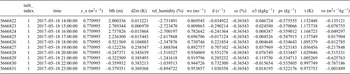


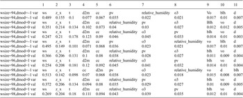


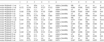


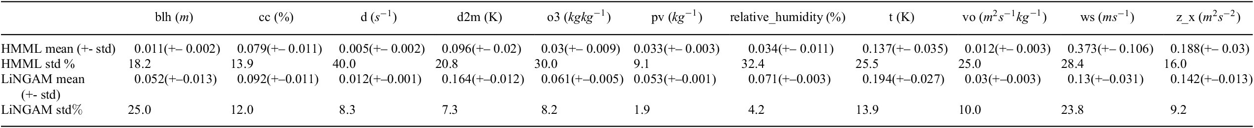

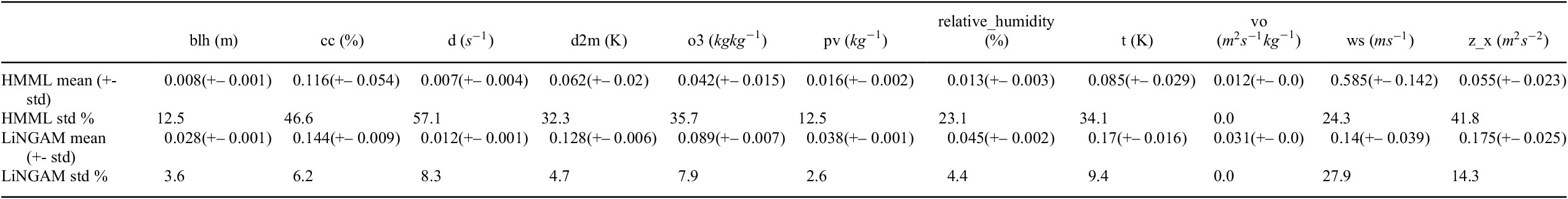

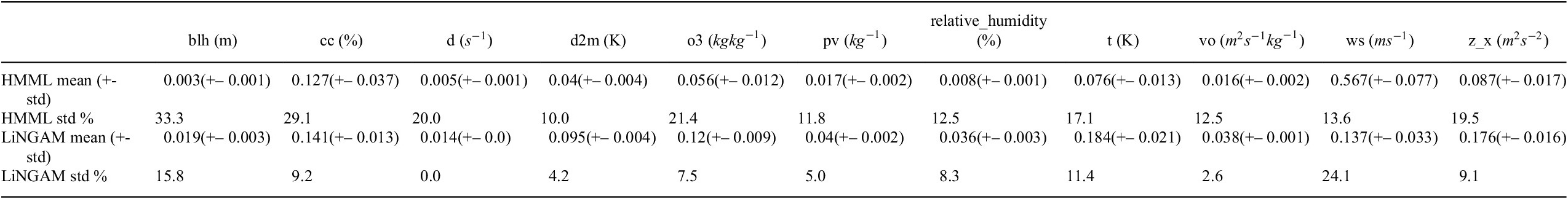

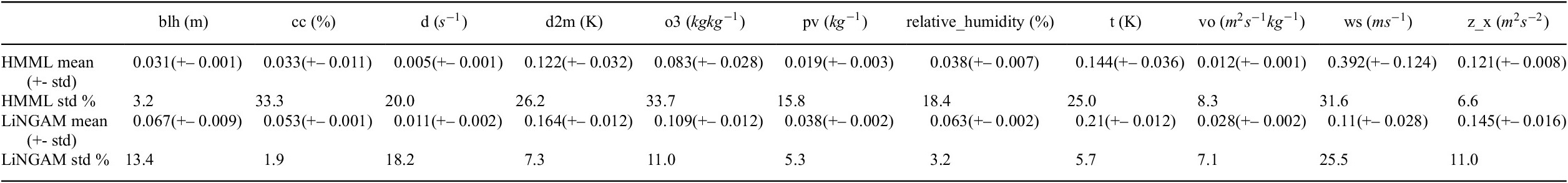

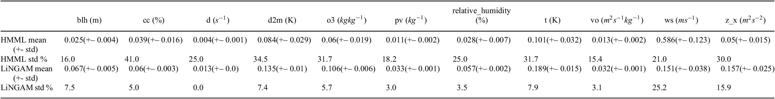

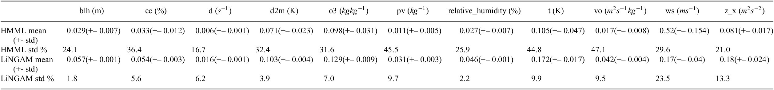


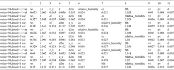


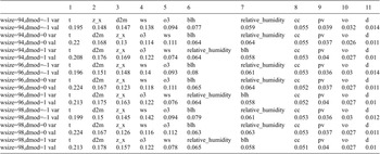


 Open access
Comments
Dear Editors-in-Chief,
We wish to submit a research article entitled “Which meteorological parameters influence extreme wind speed in a wind farm? A heterogeneous Granger causality approach” for consideration of publication in the Environmental Data Science Journal (EDS). It is a resubmission of our previously submitted paper to EDS.
The manuscript has been substantially revised based on the recommendations of both reviews.
We confirm that this work is original and has not been published elsewhere, nor is it currently under consideration for publication elsewhere.
We confirm that all co-authors are aware of the current submission and consent to its review by EDS.
We declare no conflicts of interest with any of the suggested editors or reviewers.
Thank you for your consideration of this manuscript.
With kind regards,
Katerina Schindlerova (Hlavackova-Schindler) – corresponding author
Rainer Wöss
Irene Schicker
Claudia Plant