


1. Introduction
The Taylor–Couette (TC) geometry, namely two concentric cylinders with one or both rotating, provides a tool for the rheological characterisation of complex fluids as well as a test bed for fundamental investigations of instabilities and transitions in a wide variety of flows. These range from Newtonian (Taylor Reference Taylor1923; Wereley & Lueptow Reference Wereley and Lueptow1999) to viscoelastic transitional flows and turbulence (Steinberg & Groisman Reference Steinberg and Groisman1998), suspension (Baroudi, Majji & Morris Reference Baroudi, Majji and Morris2020; Moazzen et al. Reference Moazzen, Lacassagne, Thomy and Bahrani2022) and shear-thinning (Cagney, Lacassagne & Balabani Reference Cagney, Lacassagne and Balabani2020; Lacassagne, Cagney & Balabani Reference Lacassagne, Cagney and Balabani2021b) modulated dynamics, potentially combined with other effects such as temperature or pressure gradients (Leng et al. Reference Leng, Krasnov, Li and Zhong2021), altering the stability of base Couette flow (CF).
For Newtonian fluids, TC flow with only the inner cylinder rotating is known to undergo a series of extensively studied transitions when the flow becomes centrifugally unstable. These are controlled by the Reynolds number (or Taylor number,  $Ta$), which is defined as
 \begin{equation} Re=t_v\dot{\gamma}=\frac{\rho\varOmega_i r_i d}{\eta},\end{equation}
where  $\rho$ is the fluid density, $\varOmega _i$ is the rotational speed of the inner cylinder, $r_i$ is the radius of the inner cylinder, $d$ is the gap between the two cylinders, $\eta$ is the viscosity of the fluid, $t_v=\rho d^2/ \eta$ is the viscous time scale and $\dot {\gamma } =\varOmega _i r_i/d$ is the nominal shear rate in the gap.
Initially, at a critical  $Re$, axisymmetric vortex pairs are formed, separated by inflow/outflow boundaries (Taylor vortex flow (TVF)), as exemplified in the seminal work of Taylor a century ago (Taylor Reference Taylor1923). As inertia increases (ramp-up), the vortex boundaries become unstable, oscillating with one (wavy TVF (WTVF)) (Wereley & Lueptow Reference Wereley and Lueptow1998; Akonur & Lueptow Reference Akonur and Lueptow2003) or two (modulated WTVF) (Gollub & Swinney Reference Gollub and Swinney1975; Fenstermacher, Swinney & Gollub Reference Fenstermacher, Swinney and Gollub1979; Gorman & Swinney Reference Gorman and Swinney1982; Zhang & Swinney Reference Zhang and Swinney1985) characteristic frequencies, gradually leading to chaotic flow states like chaotic Taylor–Vortex Flow (CTVF), wavy turbulent vortex (WTV) and, ultimately, turbulent Taylor–Vortex (TTV) (Jung & Sung Reference Jung and Sung2006; Bilson & Bremhorst Reference Bilson and Bremhorst2007; Dong Reference Dong2007; Dutcher & Muller Reference Dutcher and Muller2009; Grossmann, Lohse & Sun Reference Grossmann, Lohse and Sun2016) as $Re/Ta$ numbers keep increasing.
When viscoelasticity is introduced, typically through the addition of long polymer chains into the flow, the resulting flow states are altered due to an additional volume force acting perpendicular to the curved streamlines and termed ‘hoop stress’. The importance of the elastic effects on the flow is often expressed through either the Weissenberg number  $Wi=t_e\dot {\gamma }$ or the elasticity number $El=Wi/Re=t_e \eta / \rho d^2$, where $t_e$ is the polymer relaxation time (elastic time scale). While for low values of $El$, the transition sequence – for increasing rotational speed of the inner cylinder – remains similar to that of Newtonian fluids (Watanabe, Sumjo & Ogata Reference Watanabe, Sumjo and Ogata2006; Dutcher & Muller Reference Dutcher and Muller2011, Reference Dutcher and Muller2013), increasing elasticity leads to a number of instabilities and flow states, such as rotating standing waves/ribbons (Avgousti & Beris Reference Avgousti and Beris1993; Baumert & Muller Reference Baumert and Muller1999; Thomas, Sureshkumar & Khomami Reference Thomas, Sureshkumar and Khomami2006; Thomas, Khomami & Sureshkumar Reference Thomas, Khomami and Sureshkumar2009; Latrache, Crumeyrolle & Mutabazi Reference Latrache, Crumeyrolle and Mutabazi2012; Latrache et al. Reference Latrache, Abcha, Crumeyrolle and Mutabazi2016; Lacassagne et al. Reference Lacassagne, Cagney, Gillissen and Balabani2020), spiral vortices (Avgousti & Beris Reference Avgousti and Beris1993; Ashwin & King Reference Ashwin and King1997), flame patterns/oscillatory strips (Baumert & Muller Reference Baumert and Muller1997, Reference Baumert and Muller1999; Thomas et al. Reference Thomas, Sureshkumar and Khomami2006, Reference Thomas, Khomami and Sureshkumar2009; Martínez-Arias & Peixinho Reference Martínez-Arias and Peixinho2017; Latrache & Mutabazi Reference Latrache and Mutabazi2021), which eventually lead to turbulence.
Turbulent flow states emerge at vanishing inertia ( $Re\ll 1$) for high $El$ numbers ( $El\geq 1$); these are attributed solely to elastic effects and termed elastic turbulence (ET). For lower $El$ values ( $El<1$), such states emerge at higher $Re$ due to the interaction between inertia and fluid elasticity. The literature refers to those as elastically dominated turbulence when $Re\leq 100$, and elastoinertial turbulence (EIT) when $Re>100$ (Song et al. Reference Song, Zhu, Lin, Liu and Khomami2023b). In recent years EIT has attracted considerable attention from the scientific community, as it is associated with a modification of the coherent structures of the flow and turbulent drag reduction (TDR) (Xi & Graham Reference Xi and Graham2010a,Reference Xi and Grahamb, Reference Xi and Graham2012; Choueiri et al. Reference Choueiri, Lopez, Varshney, Sankar and Hof2021; Dubief, Terrapon & Hof Reference Dubief, Terrapon and Hof2023).
Coherent structures have been shown to dominate the dynamics of the polymeric flows. In channel flows, organised structures resembling narwhals (Morozov Reference Morozov2022; Lellep, Linkmann & Morozov Reference Lellep, Linkmann and Morozov2023) or arrowheads (Dubief et al. Reference Dubief, Page, Kerswell, Terrapon and Steinberg2022) pointing in the direction of the flow, have been reported in ET and EIT, respectively. Vortex pairs of diwhirls, also called solitons (Groisman & Steinberg Reference Groisman and Steinberg1997; Kumar & Graham Reference Kumar and Graham2000, Reference Kumar and Graham2001; Lange & Eckhardt Reference Lange and Eckhardt2001; Thomas et al. Reference Thomas, Sureshkumar and Khomami2006, Reference Thomas, Khomami and Sureshkumar2009; Martínez-Arias & Peixinho Reference Martínez-Arias and Peixinho2017) are thought to be the fundamental structural elements of viscoelastic TC flows (Steinberg Reference Steinberg2021). Closely associated with the stable diwhirl structures are the flame patterns, which are a chaotic flow state. They are both deemed to be purely elastic (Baumert & Muller Reference Baumert and Muller1997; Groisman & Steinberg Reference Groisman and Steinberg1997; Thomas et al. Reference Thomas, Sureshkumar and Khomami2006), and hence they typically emerge in highly elastic fluids.
Diwhirls were first observed experimentally by Groisman & Steinberg (Reference Groisman and Steinberg1997) using visualisation/laser Doppler velocimetry (LDA) and flame patterns by Baumert & Muller (Reference Baumert and Muller1997), using flow visualisation in the meridional plane. Although diwhirls have been observed only during the deceleration of the inner cylinder (ramp-down) due to hysteresis, the two instabilities have been considered closely linked. They both comprise pairs of vortices separated by strong inflow jets. Nevertheless, diwhirls seem to have attracted more attention compared with the flame pattern in the literature. A number of experimental (Groisman & Steinberg Reference Groisman and Steinberg1997, Reference Groisman and Steinberg2004) and numerical works (Kumar & Graham Reference Kumar and Graham2000, Reference Kumar and Graham2001; Thomas et al. Reference Thomas, Sureshkumar and Khomami2006, Reference Thomas, Khomami and Sureshkumar2009; Liu & Khomami Reference Liu and Khomami2013; Song et al. Reference Song, Wan, Liu, Lu and Khomami2021b; Lopez Reference Lopez2022) have attempted to provide a mechanistic understanding of the creation and the stability of the diwhirl structures. The latter has often been attributed to the elongation of the polymer chains in the jet-like inflow regions and the resulting asymmetry between inflow/outflow boundaries of the vortex pairs (Groisman & Steinberg Reference Groisman and Steinberg1997, Reference Groisman and Steinberg2004; Thomas et al. Reference Thomas, Khomami and Sureshkumar2009; Liu & Khomami Reference Liu and Khomami2013; Lopez Reference Lopez2022). The existence of a feedback loop between the strong radial elongation of the polymers along the centreline of the inflows, where  $\partial u_r /\partial r>0$ ( $u_r$ is the radial component of the velocity) and the increase of the hoop stress in the azimuthal direction, results in a self-sustaining mechanism for diwhirls (Groisman & Steinberg Reference Groisman and Steinberg1997; Kumar & Graham Reference Kumar and Graham2000, Reference Kumar and Graham2001; Thomas et al. Reference Thomas, Sureshkumar and Khomami2006, Reference Thomas, Khomami and Sureshkumar2009) and is considered the driving mechanism of ET by Song et al. (Reference Song, Lin, Zhu, Wan, Liu, Lu and Khomami2023a,Reference Song, Zhu, Lin, Liu and Khomamib).
Recently, Lopez (Reference Lopez2022) showed numerically that flame patterns and diwhirls comprise the same coherent structures but with different dynamics and used the term diwhirls to describe both. He demonstrated that the interaction between different diwhirls, either stable or unstable (flame pattern), is governed by two-dimensional elastic effects, leading to the decoupling of their dynamics, allowing them to move independently, leading to EIT. Neither hysteresis nor the pre-existence of rotating standing waves were found to be necessary conditions for the formation of diwhirl structures.
Despite the extensive numerical works on the transitional flows and EIT in TC (Song et al. Reference Song, Zhu, Lin, Liu and Khomami2023b), experimental investigations are limited. In most reported studies, flow visualisation experiments are commonly employed to elucidate the transitions (Boulafentis et al. Reference Boulafentis, Lacassagne, Cagney and Balabani2023). To date, and to the best of our knowledge, no study has experimentally resolved the spatiotemporal flow characteristics of diwhirls and flame patterns, establishing their connection and revealing their link to EIT. This is despite an abundance of mechanisms and pathways to EIT observed experimentally for TC flows, such as (vortex) merging and splitting transition (MST/VMS) (Lacassagne et al. Reference Lacassagne, Cagney, Gillissen and Balabani2020; Song et al. Reference Song, Wan, Liu, Lu and Khomami2021b; Lopez Reference Lopez2022), defect-mediated turbulence (Latrache et al. Reference Latrache, Abcha, Crumeyrolle and Mutabazi2016) and disordered oscillations (Groisman & Steinberg Reference Groisman and Steinberg1996) to name but a few.
To address this, we experimentally studied the highly elastic transition to turbulence through flame patterns. We investigate the dependence of flame structures on fluid elasticity and the role of hysteresis on the route to EIT using visualisation experiments. We perform particle image velocimetry (PIV) measurements in selected regimes, covering the three main instabilities observed in our visualisation experiments, namely diwhirls, flame patterns and EIT. These allow us to resolve the flow field and elucidate the key mechanisms and coherent structures governing the dynamics of the observed flow states. The geometrical parameters of the TC cell, the rheological properties of the viscoelastic fluids used in this work and the visualisation/PIV protocols, are introduced in § 2. The visualisation and PIV results along with the spectral characteristics obtained from both are then presented in § 3. Section 4 discusses the findings and proposes a generalised mechanism on the effect of the viscoelasticity on the flow instabilities, while § 5 concludes the study.
2. Materials and methods
2.1. The TC geometry
A TC flow cell (figure 1), previously used in Cagney et al. (Reference Cagney, Lacassagne and Balabani2020) and Lacassagne et al. (Reference Lacassagne, Cagney, Gillissen and Balabani2020, Reference Lacassagne, Boulafentis, Cagney and Balabani2021a,Reference Lacassagne, Cagney and Balabanib), was constructed comprising two concentric cylinders; the inner one is made of PTFE (polytetrafluoroethylene) and the outer one of a transparent acrylic material. The inner cylinder is painted black to avoid reflections during illumination and to achieve a smooth surface. It features a conical-shaped tip at the bottom, sitting inside an indent in the lower plate and a shaft at the top, mounted on a ball-bearing at the upper plate to reduce friction and a potential temperature rise and ensure cylinder alignment. A stepper motor (SmartDrive Ltd, Cambridge, UK), with a high resolution of 52 000 microsteps/revolution, was mounted on the inner cylinder shaft, allowing precise control of the rotational speed/acceleration. The radii of the inner and outer cylinders are  $r_i=21.66$ mm and $r_o=27.92$ mm, respectively, and their height $H=135$ mm. These parameters result in a gap between the two cylinders of $d=6.26$ mm, a radius ratio of $\eta _{cell}=r_i / r_o =0.77$, an aspect ratio $\varGamma =H / r_i =21.56$ and a curvature of $\epsilon =d / r_i=0.29$. The working fluid is carefully poured between the two cylinders to avoid entrainment that may lead to a free surface. The cell is enclosed in a rectangular container, connected to a cooling system. The continuous recirculation of water at a constant temperature of $20\,^\circ$C enables the temperature of the working fluids to be accurately controlled during the experiments, with a maximum deviation of $0.1\,^\circ$C.

Figure 1. The TC cell with the flow visualisation (a) and the PIV set-up (b).
2.2. Preparation of polymer solutions and characterisation
A viscous solvent comprising  $72\,\%$ glycerol and $28\,\%$ deionised water was selected for consistency with previous works of our group (Lacassagne et al. Reference Lacassagne, Cagney, Gillissen and Balabani2020, Reference Lacassagne, Cagney and Balabani2021b) and a high molecular weight polyacrylamide (PAAM) polymer (Sigma-Aldrich, $M_w=5.5\times 10^6~\mathrm {g}~\mathrm {mol}^{-1}$) was added at different concentrations to introduce elasticity.
Since PAAM is soluble in water but not in glycerol (Hopkins et al. Reference Hopkins, Gogovi, Weisel, Handler and Blaisten-Barojas2020), to prepare the solutions, it was first dissolved in deionised water by natural diffusion at room temperature for 24 hr, then stirred and mixed with the desired glycerol volume. The final mixture was then shaken until a homogeneous solution was achieved, as suggested by Soares et al. (Reference Soares, Silva, Andrade and Siqueira2020).
Different polymer solutions were produced by varying PAAM concentrations from  $350$ to $1000$ p.p.m. and their shear viscosity was measured using a rotational rheometer (ARES rheometer, TA instruments) using a Couette geometry ( $r_i=32$ mm, $r_o=34$ mm) at $20\,^\circ$C. Three sets of measurements were acquired for each solution to minimise both loading and instrument errors. Figure 2(a) shows the steady shear viscosity curves for the PAAM solutions studied. The inset shows normal stresses measured in the same rheometer for the case of $c=1000$ p.p.m.; a plate–plate geometry was used with a diameter of $D=50$ mm and a gap of $d=1$ mm in this case.

Figure 2. (a) Steady-shear rheological properties of PAAM solutions of different concentrations. In the inset, the normal stress is plotted against the shear rate for the case of  $1000$ p.p.m. (b) Filament diameter evolution for different PAAM concentrations. Here IC and EC denote the inertiocapillary and elastocapillary thinning regimes, respectively. The solvent is the same for all cases, 72 % glycerol and 28 % water.
The shear viscosity data were fitted by the Carreau model,
 \begin{equation} \eta(\dot{\gamma})=\eta_{\infty}+(\eta_{0}-\eta_{\infty})(1+(t_c \dot{\gamma})^2)^{(n_c-1)/2}, \end{equation}
where  $\eta _{\infty }$ and $\eta _{0}$ are the infinite and zero shear-rate viscosities, respectively, $t_c$ is the Carreau model time scale and $n_c$ the flow index.
The solutions have almost constant viscosity for low concentrations of PAAM, but they become progressively more shear-thinning for higher concentrations due to the entanglement of the polymer chains. The extent of shear-thinning was evaluated using the average gradient of the viscosity curve (Cagney et al. Reference Cagney, Lacassagne and Balabani2020; Lacassagne et al. Reference Lacassagne, Cagney and Balabani2021b),
 \begin{equation} \bar{n}_e=\frac{\partial \log(\eta)}{\partial \log(\dot{\gamma})}+1,\end{equation}
which provides more consistent results than the Carreau-model derived flow index  $n_c$. The values of $\bar {n}_e$ are listed in table 1. The polymer solutions exhibiting significant shear-thinning ( $\bar {n}_e<0.95$, table 1), namely $c=1500$ p.p.m. and $c=2000$ p.p.m., were excluded from the visualisation and PIV experiments shown later.
Table 1. A summary of the rheological properties of the fluids examined in this work.

The critical overlap polymer concentration in the current work was evaluated using three methods: (i) the calculation of the intrinsic viscosity  $[\eta ] ([\eta ]=0.00107)$ and Grassley's equation $c^*=0.77/[\eta ]$ ( $c^*=718$ p.p.m.), (ii) the Solomon–Ciută equation ( $c^*=687 \pm 60$ p.p.m.) and (iii) the calculation of the concentration at which the viscosity contribution of the polymers is equal to that of the solvent ( $\eta _s=\eta _p$) which works as an extra validation of the method ( $c^*\cong 700$ p.p.m.) (Schafer Reference Schafer2013). All three methods resulted in $c^*\approx 700$ p.p.m. within 13 % (more information in Appendix A). According to Rubinstein & Colby (Reference Rubinstein and Colby2003), entanglement occurs in concentrations $c^{**}$ in the range $4< c^{**} / c^*<30$ which are well above those used in the present work, hence all polymer solutions used were either in the dilute or slightly semidilute regime.
Extensional measurements were obtained to determine the polymer relaxation time in a bespoke set-up utilising the slow retraction method (Campo-Deaño & Clasen Reference Campo-Deaño and Clasen2010; Sousa et al. Reference Sousa, Vega, Sousa, Montanero and Alves2017) implemented in the rheometer. The elongational relaxation time has been considered to be the most suitable for the jet-dominated dynamics of the flows presented later in this work (§ 3), as suggested by Bai et al. (Reference Bai, Latrache, Kelai, Crumeyrolle and Mutabazi2023).
A summary of the rheological properties of all the fluids used in this work is provided in table 1. The polymer solutions are named using the convention in Lacassagne et al. (Reference Lacassagne, Cagney and Balabani2021b): N denotes a Newtonian solution, (N(WGL-72) the solvent and N(W) deionised water), PAAM the Boger fluids and the accompanying number denotes the polymer concentration in parts per million (p.p.m.). The parameters of the Carreau model ( $\eta _{0}$, $\eta _{\infty }$, $n_c$, $t_c$), the effective shear-thinning index $\bar {n}_e$, the relaxation time as extracted from extensional measurements $t_e$, the viscosity ratio $\beta =\eta _p/ \eta$ and the average elasticity ( $\overline {El}$) define each polymer solution.
As the viscosity of Boger fluids is almost constant, the elasticity number varies only slightly with the shear rate and Reynolds number and each fluid can be characterised using only the average value of the elasticity number,  $\overline {El}$. Thus, hereafter, the elasticity number $El$ refers to the average value. All fluid solutions lie in the moderately elastic regime, $0.1< El<1$. It should be noted, however, that $El$ depends on the measured relaxation time, which can vary depending on the estimation method. Extensional measurements tend to result in lower relaxation times and therefore lower elasticity numbers (Boulafentis et al. Reference Boulafentis, Lacassagne, Cagney and Balabani2023).
The density of the solutions was considered independent of the polymer concentration and equal to the density of the solvent  $\rho =1198~\mathrm {kg}~\mathrm {m}^{-3}$.
2.3. Flow visualisation experimental protocol
The flow transitions for the different polymer solutions were visualised using our previously developed experimental protocol, described in detail in Cagney et al. (Reference Cagney, Lacassagne and Balabani2020) and Lacassagne et al. (Reference Lacassagne, Cagney, Gillissen and Balabani2020, Reference Lacassagne, Boulafentis, Cagney and Balabani2021a,Reference Lacassagne, Cagney and Balabanib). Briefly, the flow was seeded with  $0.01\,\%v / v$ reflective mica flakes (Cornelissen & Son, Pearl Lustre Pigments), 10–100 $\mathrm {\mu }$m in diameter, illuminated by two light-emitting diode (LED) lights (PHLOX) and imaged using a high-speed camera (Phantom Miro M340) as shown in figure 1. A large number of images $O(10^5)$ of a thin strip, $2176$ pixels spanning the height of the TC cell and $16$ pixels in the azimuthal direction ( $2176\times 16$ pixels) (figure 1a), were recorded. These are averaged vertically creating $2176\times 1$ pixel columns of instantaneous intensity values $I$ and are compiled to create spatiotemporal maps, showing the evolution of $I$ with time ( $x$-axis), along the height $H$ of the TC cell ( $\kern 1.5pt y$-axis) (Cagney et al. Reference Cagney, Lacassagne and Balabani2020; Lacassagne et al. Reference Lacassagne, Cagney, Gillissen and Balabani2020, Reference Lacassagne, Boulafentis, Cagney and Balabani2021a,Reference Lacassagne, Cagney and Balabanib). The same maps can be expressed in terms of $Re$ as the inner cylinder rotational speed varies. The intensity values are first inverted so that the highest values correspond to strong radial velocities and normalised using the maximum and minimum values of each map so that $I\in [0,1]$ with 0 corresponding to a purely azimuthal flow like CF (no radial velocity) and 1 to a strong radial flow (no azimuthal component).
On the top and bottom of the TC cell, Ekman vortices and instabilities are formed due to boundary conditions (Ekman Reference Ekman1905; Sobolík et al. Reference Sobolík, Izrar, Lusseyran and Skali2000). To exclude them from the spatiotemporal maps, only the area between 0.1 and 0.9 of the total height is illustrated in the maps.
Three types of visualisation experiments were performed: (i) for accelerating inner cylinder (ramp-up); (ii) for decelerating inner cylinder (ramp-down); (iii) for constant rotational speed (steady-state). A non-dimensional acceleration/deceleration  $\varGamma _0=0.3$ was used in all experiments, well below the critical limit ( $\varGamma _0<1$), to ensure quasistatic conditions (Xiao, Lim & Chew Reference Xiao, Lim and Chew2002; Dutcher & Muller Reference Dutcher and Muller2009; Lacassagne et al. Reference Lacassagne, Cagney and Balabani2021b). Here $\varGamma _0$ is defined as
 \begin{equation} \varGamma_0=\frac{{\rm d} Re}{{\rm d} \tau}=\frac{\rho^2r_id^3}{\eta^2}\frac{{\rm d} \varOmega}{{\rm d} t},\end{equation}
where  $\tau =t / t_v$ is the non-dimensional time based on the viscous time scale $t_v=\rho d^2 / \eta$. It should be noted that by definition $\varGamma _0$ is inversely proportional to the square of the solution viscosity, $\varGamma _0 \propto 1 / \eta ^2$, implying that for shear-thinning solutions, it varies nonlinearly with rotational speed (Dutcher & Muller Reference Dutcher and Muller2013; Lacassagne et al. Reference Lacassagne, Cagney and Balabani2021b). However, the viscosity of the working fluids in the present work remains constant in the range of applied deformation studied (Boger fluids) and hence $\varGamma _0$ can be assumed constant.
The Reynolds number was varied from 0–200 to minimise polymer mechanical degradation due to scission (Vazquez et al. Reference Vazquez, Schmalzing, Matsudaira, Ehrlich and McKinley2001) and ensure repeatability of results. To this end, each polymer solution was used for one set of ramp-up and ramp-down experiments only, following the same protocol for consistency, and the steady-shear rheology of the solutions was measured before and after each visualisation experiment (also in the presence and absence of flakes). Selected flow curves are shown in Appendix B. In addition, an extra ramp-up experiment was always performed after the first series of experiments and was compared with the initial ramp-up test to ensure that the critical Reynolds numbers and the transitions were unchanged.
The acquisition frequency,  $f_a$, used for the visualisation experiments was kept high ( $\,f_a=80\unicode{x2013}230$, dictated by the camera memory), to resolve the transitions with the greatest temporal resolution possible. The temporal resolution of the flow maps is determined by the variation of Reynolds number per frame, $\Delta Re$. The number of frames per Reynolds number, $1 / \Delta Re$ ranged between $336\unicode{x2013}542$ in our experiments (table 2).
Table 2. A summary of the experimental settings for the visualisation experiments.

Flow transitions were determined by changes in the root mean square (r.m.s.) of intensity  $i^*={\rm r.m.s.}(I)$ along the height of the TC cell. The onset of EIT was determined by the saturation of the number of flames (see § 3.1.2), counted using a custom-made MATLAB code utilising a combination of image binarisation and processing based on the intensity histogram of the flow maps. The saturation of the number of flame patterns was also evident in the saturation in the value of $i^*$ most of the time.
Frequency maps were also employed to identify the flow transitions. The spatiotemporal matrix is divided into sections of  $1024$ columns with $87\,\%$ overlap and the fast Fourier transformation (FFT) is calculated for every row (spatial position along the height $H$). The averaged FFT signal across $H$ for each of these sections was compiled into a contour map of the frequency signal strength. Using this map, the evolution of the flow frequencies for increasing/decreasing $Re$ could be monitored. For spatial FFT, every column is a spatial signal of $2176$ pixels, sampled at a rate of $2176 / \varGamma$. The peak of the FFT in the spatial dimension corresponds to the normalised wavenumber $d / \lambda$, which is equal to the dominant spatial frequency.
2.4. The PIV experimental protocol
The PIV measurements were performed along the  $r$–
$r$– $z$ plane of the annular gap in the region spanning from $z / d=-6$ to $z / d=6$, with $z / d=0$ taken at midheight (figure 1b). The field of view had to be held large enough to enable the observation of the large-scale flame pattern/diwhirl structures and their evolution as they appear and interact at random axial locations.
Steady-state and ramp-up measurements were acquired. Steady-state experiments were used to resolve the flow field at a fixed  $Re$ number. The inner cylinder was accelerated or decelerated until the desired Reynolds number was achieved and was then held constant. The PIV measurements during ramp-up were used to capture the transient dynamics of the flow for varying $Re$. In that case, the acquisition of the images was initiated at a desired Reynolds number and continued as the rotational speed of the inner cylinder was slowly accelerated (with the same acceleration as the one used in the visualisation experiments $\varGamma _0=0.3$) up to the next Reynolds number of interest. The acquisition settings (table 3) were adjusted to achieve high temporal resolution of the transient dynamics of the flow ( $293$ flow fields per $Re$).
Table 3. A summary of the experimental settings for the PIV experiments.

In all cases, silver-coated hollow glass spheres (S-HGS-10, Dantec Dynamics) with an average diameter of 10  $\mathrm {\mu }$m were used as tracer particles (Stokes number, $Stk<0.03$), added to the solutions just before the experiments in very small concentrations ( $0.008\,\%v / v$). The flow was illuminated using a continuous laser of 532 nm wavelength (LRS-0532 DPSS laser, Laserglow, CA), producing a laser sheet of 1 mm thickness (figure 1b). Particle images (table 3) were acquired using a Phantom Miro M340 camera (Vision Research), either in single or double-frame acquisition mode. The acquisition frequency used for double-frame measurements was either $f_a=100$ Hz or $f_a=410$ Hz (table 3). The time between the two image pairs, $dt$, was adjusted so that the number of invalid vectors was minimised ( $<3\,\%$). In single-frame experiments, a high frequency of $f_a=2151$ Hz was implemented to resolve the fast-moving flows and chaotic dynamics of EIT. The acquisition and PIV processing of image pairs was performed using a commercial software (Dynamic Studio, Dantec Dynamics). A multipass adaptive PIV scheme followed by a $3\times 3$ moving average validation and average filter was employed resulting in $12\times 145$ vectors in the radial and axial directions, respectively. The instantaneous radial and axial velocities were extracted and decomposed into time-averaged and fluctuating parts $u_r=\bar {u}_r + u_r'$, $u_z=\bar {u}_z + u_z'$. The azimuthal vorticity $\varOmega _{\theta }$ was calculated at every point $(i,j)$ using the circulation (eight-point) method of differencing (Raffel et al. Reference Raffel, Willert, Scarano, Kähler, Wereley and Kompenhans2018).
Tables 2 and 3 summarise the experimental settings used for the visualisation and PIV experiments, respectively.
3. Results
3.1. The elastoinertial transition maps
This section provides an overview of the flow transitions observed for the various fluid elasticities, examined based on spatiotemporal maps produced from the experiments summarised in table 2. For all experimental sets, the transitions were monitored both for ramp-up and for ramp-down of the inner cylinder.
3.1.1. Overview of the transitions
Phase diagrams of the observed flow states as a function of  $El$ are shown in figures 3(a) and 3(b) for ramp-up and ramp-down experiments, respectively. The critical $Re$ are summarised in table 4.

Figure 3. Overview of the flow states as a function of the elasticity number  $El$ for (a) ramp-up and (b) ramp-down.
Table 4. A summary of the critical Reynolds numbers for fluids of various  $El$ numbers. DW, diwhirls; RSW, rotating standing waves; FP, flame patterns.

In the Newtonian case, the flow undergoes the extensively studied, non-hysteretic transition of CF $\rightarrow$TVF $\rightarrow$WTVF with a wavelength of $\lambda /d=1.7$ in both TVF and WTVF, similar to Dutcher & Muller (Reference Dutcher and Muller2013). The critical Reynolds numbers for TVF and WTVF are 101 and 197, respectively, in agreement with the literature. Critical values are, however, dependent on the geometrical parameters and the experimental protocols employed (Andereck, Liu & Swinney Reference Andereck, Liu and Swinney1986; Wereley & Lueptow Reference Wereley and Lueptow1998; Ostilla-Mónico et al. Reference Ostilla-Mónico, Poel, Verzicco, Grossmann and Lohse2014; Ramesh, Bharadwaj & Alam Reference Ramesh, Bharadwaj and Alam2019).
When the elasticity number exceeds a critical value of  $El_{cr}\cong 0.11$ (figure 3 for $El=0.11\unicode{x2013}0.34$), the flow transition becomes elastically modified; it is characterised by a CF $\rightarrow$rotating standing waves $\rightarrow$flame patterns $\rightarrow$EIT pathway in ramp-up experiments and EIT $\rightarrow$flame patterns $\rightarrow$diwhirls $\rightarrow$CF during ramp-down, as illustrated in figure 4 (for $El=0.34$) showing typical flow and frequency maps as well as the variation of $i^*$, marking the flow transitions.

Figure 4. Typical r.m.s. of intensity ( $i^*={\rm r.m.s.}(I)$) (a,b), frequency maps (c,d) and spatiotemporal maps (e, f), used for the analysis of flow transitions in ramp-up (a,c,e) and ramp-down (b,d, f) experiments for $El=0.34$.
Increasing fluid elasticity further does not change the transitional sequence in both ramp-up and ramp-down experiments (figure 3).
In all cases, during ramp-up, CF gives rise to rotating standing waves for a very narrow  $Re$ range, followed by a quick merge of the elastic waves into strong radial inflows of the flame patterns (figures 3a and 4e). In contrast to rotating standing waves, flame patterns do not exhibit a frequency signature, as is evident in figures 4(c) and 4(d), due to the highly chaotic nature of the instability. The same applies to the wavelength, as the peaks of the spatial spectra vary greatly based on the number of the flames merging events (not shown). This indicates that the flame pattern is a chaotic mechanism like MST, which leads to EIT. However, the governing dynamics of the flame pattern qualitatively differ from MST, as will be discussed in the next sections.
In the ramp-down experiments (figures 3b and 4b,d, f) an abrupt transition from EIT to an intermediate state of flame patterns is observed ( $Re_{rd}^{EIT}=200$) as $Re$ decreases (observed in the linear $i^*$ curve, further supported later based on the number of flames), exhibiting reverse hysteresis (i.e. $Re_{ru}^{EIT}< Re_{rd}^{EIT}$). The flame pattern structures are followed by hysteretic stationary structures of diwhirls, initially superimposed with rotating standing waves, quickly replaced by a purely azimuthal flow in the areas between the radial inflows until the diwhirl structures are annihilated, leading to CF.
The critical  $Re$ for both the primary and secondary bifurcations reduces as $El$ increases, leading to an earlier onset of elastic instabilities. Interestingly, the critical $Re$ for the primary bifurcation (rotating standing waves and diwhirls) is almost the same in both ramp-up and down experiments for each fluid, regardless of the fluid elasticity (figure 5), indicating a supercritical transition, in contrast with published works (Groisman & Steinberg Reference Groisman and Steinberg2004; Martínez-Arias Reference Martínez-Arias2015; Martínez-Arias & Peixinho Reference Martínez-Arias and Peixinho2017). This could be attributed to differences in the fluids (different polymers, different $\beta$), ramping protocols and geometrical TC cell parameters employed. The critical Reynolds number for the onset of EIT decreases during the ramp-up (figure 3a), but remains unaffected in ramp-down, $Re_{rd}^{EIT}=200$ (figure 3b).

Figure 5. Zoomed spatiotemporal maps around the critical  $Re$ of the primary bifurcation for fluids of different $El$: (a) for $El=0.11$, (i) ramp-up and (ii) ramp-down; (b) for $El=0.13$, (i) ramp-up and (ii) ramp-down; (c) for $El=0.22$, (i) ramp-up and (ii) ramp-down; (d) for $El=0.34$, (i) ramp-up and (ii) ramp-down. The triangles indicate either ramp-up or ramp-down protocol. RSW, rotating standing waves.
Fluid elasticity appears to stabilise the elastically induced structures (flame patterns, diwhirls) as indicated by the easier-to-distinguish flame and diwhirl structures in figure 5, and determines the number of diwhirls: four and five unevenly distributed and highly unstable diwhirls are observed for  $El=0.11$ and $El=0.13$, respectively (figures 5aii and 5bii). When elasticity increases to $El=0.22$, five almost equally spaced diwhirls are observed with an average distance between their centres $\cong 3.5d$ (figure 5cii); they increase to seven when $El=0.34$, spaced at $2.5d$ (figure 5dii). The distance of the diwhirl centres in the present work is lower than the stability limit of $5d$ reported by Groisman & Steinberg (Reference Groisman and Steinberg1997) and the diwhirls remain stable as the flow reverts to CF. This can be attributed to the decreasing $Re$ nature of our ramping experiments as opposed to the very long, steady-state experiments on which previous observations are based.
3.1.2. The flame pattern modes in the route to turbulence
To further probe the structure and evolution of the instabilities with elasticity, the spatiotemporal maps were binarised and skeletonised as shown in figure 6 to clearly distinguish the flames. It can be seen that the evolution of the flame pattern is characterised by random events of flame creation, merging when they approach each other and annihilation, possibly when the hoop stress is not sufficient to sustain the inflow jets (marked in figure 6 with hexagon, diamond and circular markers, respectively). This mechanism, creation, merging and annihilation (CMA), qualitatively differs from the MST mechanism reported by both Lacassagne et al. (Reference Lacassagne, Cagney, Gillissen and Balabani2020) and Lopez (Reference Lopez2022) in that it incorporates the annihilation of the vortex pair structures, usually followed by an almost immediate creation event, instead of their splitting. This difference has significant consequences on the stability of the flames as they can be considered self-sustained structures (Kumar & Graham Reference Kumar and Graham2000, Reference Kumar and Graham2001) which when formed, move and interact as one entity.

Figure 6. Zoomed and skeletonised snapshots of the spatiotemporal map in figure 4(e) for  $El=0.34$. Black lines denote the flame structures (regions of inflow jets). Events of creation, merging and annihilation of flames are highlighted with hexagon, diamond and circular markers, respectively.
The frequency of CMA events increases during the ramp-up, leading to progressively more chaotic flame patterns with an increased number of flames,  $\langle n \rangle$. The latter follows a power-law growth $\langle n \rangle =10.48 \times (Re\unicode{x2013}Re_{cr})^{0.23}$ (figure 7a), in good agreement with Latrache & Mutabazi (Reference Latrache and Mutabazi2021) and Lemoult et al. (Reference Lemoult, Shi, Avila, Jalikop, Avila and Hof2016) who connected it to the directed percolation of the turbulent phase in shear flows. The number of flames stabilises after the onset of EIT reaching a plateau value of $\langle n_{EIT} \rangle =26.57$, not far from the value of $\langle n_{EIT} \rangle =24$ reported by Latrache & Mutabazi (Reference Latrache and Mutabazi2021), despite the differences in the aspect ratio between the two works.

Figure 7. Evolution of the number of flames with  $Re$, for values above the critical $Re_{cr}$ for the onset of the primary bifurcation in the case of (a) ramp-up and (b) ramp-down. The data points in (a) are fitted by a power law function up to the saturation of the number of flames in EIT. During ramp-down, two linear regimes, separated by a discontinuity can be discerned.
During ramp-down (figure 7b), the flow transitions immediately to an intermediate state at which the number of flames decreases linearly  $\langle n \rangle =0.6447\times (Re\unicode{x2013}Re_{cr}$). The linear relationship between the number of flames and $Re$ indicates that the rotational speed of the inner cylinder becomes the key parameter in this case, due to its linear relationship with the hoop stresses. After a critical $Re$, close to $25\leq (Re\unicode{x2013}Re_{cr})\leq 30$, a discontinuity in figure 7(b) emerges. This indicates the importance of hysteresis and a fundamental difference in the mechanism of the creation/evolution of flame between ramp-up/ramp-down, as will be discussed later.
Differences in the flame pattern structure between ramp-up and down experiments are clearly illustrated in the steady-state spatiotemporal maps for the most elastic case ( $El=0.34$) shown in figure 8 produced from steady-state experiments. Figure 8(a–c) shows selected flame pattern flow states of increasing number of flames, leading to EIT (figure 8d), whereas figure 8(e–g), the corresponding deceleration states (i.e. at the same $Re$ number). For example, it can be seen that the flame pattern in figure 8(e) exhibits a clearer branching structure and a smaller number of flames than its equivalent during ramp-up (figure 8c). We term this linear flame pattern (LFP), due to its linear decrease in number, a trend that is also evident in the $i^*$ profiles (figure 4b). The flow state corresponding to the discontinuity point in the number of flames during ramp-down (figure 7) is shown in figure 8( f). It comprises a transitional flow characterised by a superposition of flame pattern with non-rotating standing waves, stabilising and destabilising in different axial locations. Although this instability makes its appearance only during the deceleration of the inner cylinder, it resembles the flame pattern in the case of low-elasticity fluids, close to $El_{cr}$; we thus term this pattern elastic standing waves (ESW). Finally, figure 8(g) illustrates the flow state close to the critical $Re$ for the appearance of diwhirls. A coexistence of diwhirls, flame patterns, rotating standing waves and spirals is apparent, implying that the appearance and preservation of diwhirl structures are local and the location can vary for the same $Re$. The fact that stable diwhirl structures can only be formed during ramp-down, implies that diwhirls cannot be formed from CF/rotating standing waves; instead, they appear through a stabilisation process of already present flame pattern structures, a mechanism explained in a later section of this work.

Figure 8. Spatiotemporal maps from steady-state experiments, showing the evolution of the flow for 50 s (for  $El=0.34$) (a–c) ramp-up and (e–g) ramp-down. Panel (d) corresponds to EIT.
Flames are always separated by either rotating standing waves or spirals at low  $Re$, whereas diwhirls are separated by CF when stabilised. Interestingly, spiralling waves seem to stem from the flame pattern cores (figure 8a,g appearing as oscillations around the inflows), meaning that the unstable elongational flow of the polymers in the centre of the flames can produce elastic oscillations under certain conditions which will be further explored in the next section.
3.2. Flow fields of highly elastic states
The kinematics of the main states revealed by the visualisation experiments (diwhirls, flame patterns and EIT) as well as the onset of flame patterns from CF were characterised by PIV for the most elastic fluid (1000 p.p.m.,  $El=0.34$). In order to probe their nature, we resolve the coherent structures of the flows, assess their stability and elucidate their dynamics, governed by the CMA mechanism.
3.2.1. Resolving the coherent structures
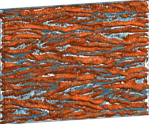
Figure 9 illustrates velocity vector fields, averaged over one rotation of the inner cylinder with streamwise vorticity contours superimposed for the cases of diwhirls ( $Re=68$), flame patterns ( $Re=80$) and EIT ( $Re=200$). The Newtonian case ( $El=0$) of TVF ( $Re=140$) is also shown for comparison. Coherent structures of solitary pairs of vortices can be observed in the three viscoelastic cases. These vortex pairs have reduced axial wavelength compared with the Newtonian ones ( $\lambda _{DW}\approx d$, $\lambda _{TVF}\approx 2d$), their cores are shifted close to each other and have a clear boundary of strong, narrow inflow jets. They are separated by plain CF in the case of diwhirls, spaced at a distance of $\approx 7d$ (figure 9b), whereas they are present throughout the flow domain in the case of flame patterns and EIT (figure 9c,d). In the case of EIT, the importance of the outflow boundaries increases, leading to pairs that are not spatially locked in the radial direction but can also be located close to the outer, stationary wall. Some of the vortex pairs exhibit a seemingly weaker vorticity and less defined structure which could be due to either smaller hoop stresses in the azimuthal direction or their neighbouring pairs dominating the angular momentum transfer process. No Görtler vortices have been observed close to the inner cylinder as reported by Song et al. (Reference Song, Teng, Liu, Ding, Lu and Khomami2019), which can be attributed to the small gap ratio employed here (Song et al. Reference Song, Teng, Liu, Ding, Lu and Khomami2019, Reference Song, Wan, Liu, Lu and Khomami2021b).

Figure 9. Velocity vectors with contours of the azimuthal vorticity, normalised by the rotational speed of the inner cylinder  $\varOmega _\theta / \varOmega _i$. The velocity fields are averaged through one rotation of the inner cylinder to ‘freeze’ the flow and resolve the coherent structures of (a) TVF, $Re=140$; (b) diwhirls, $Re=68$; (c) flame patterns, $Re=75$; (d) EIT, $Re=200$. Panel (a) is for a Newtonian fluid (WGL-72) and (b–d) for $El=0.34$.
The average velocity profiles of both the axial ( $\bar {u}_z$) (figure 10a,b) and radial ( $\bar {u}_r$) (figure 10c,d) components along the middle of the gap are similar between the three instabilities (diwhirls, flame patterns, EIT). Although vortex pairs can be located in all three cases, due to the interaction of the structures in the most chaotic states, it is more difficult to discern their characteristic profiles. These interactions lead to reduced strength at the outflows of the neighbouring vortices, not observed in previous works (Groisman & Steinberg Reference Groisman and Steinberg1997, Reference Groisman and Steinberg1998). Nevertheless, the radial velocity profiles of diwhirls are consistent with those obtained experimentally using LDA by Groisman & Steinberg (Reference Groisman and Steinberg1997, Reference Groisman and Steinberg1998) and numerically by Kumar & Graham (Reference Kumar and Graham2001) and Thomas et al. (Reference Thomas, Sureshkumar and Khomami2006, Reference Thomas, Khomami and Sureshkumar2009). The spatial resolution of the published LDA measurements is lower than the PIV ones reported here, which might explain the differences in the outflows.

Figure 10. Profiles of (a) axial ( $\bar {u}_z$) and (c) radial components ( $\bar {u}_r$) of the velocities across the middle of the gap $(r_o-r_i)/2$, for the different flow states: TVF, $Re=140, El=0$); diwhirls, $Re=68, El=0.34$; flame patterns, $Re=80, El=0.34$; EIT, $Re=200$, $El=0.34$. The profiles of (b) $\bar {u}_z$ and (d) $\bar {u}_r$ are shifted and aligned to the position of the inflow boundary of the vortices $z^*=z-z_s$ to facilitate the comparison. In (d), the analytical solution of the soliton is fitted in the experimental data, denoted by the dashed line.
Following the work of Latrache & Mutabazi (Reference Latrache and Mutabazi2021), we fit the analytical soliton equation to the diwhirl averaged radial velocity profile in the middle of the gap (figure 10d),
 \begin{equation} V_{sol}=A-B \textit{sech}\left(\frac{z-z_s}{C}\right),\end{equation}
where A, B and C are free-fitting parameters and  $z_s$ is the axial position of the centre of the soliton. The fitting proves very close to the experimental data of the inflow jet but is unable to capture the peaks of the outflow boundaries.
From the velocity profiles, the inflow width in the gap centreline is estimated to be equal to  $0.56d$, comparable to the values in experimental (Groisman & Steinberg Reference Groisman and Steinberg1997) and numerical (Lange & Eckhardt Reference Lange and Eckhardt2001; Thomas et al. Reference Thomas, Sureshkumar and Khomami2006) studies. The ratio between the inflow and outflow maximum radial velocities is $2.2$ in our experiments, lower than the reported values by Groisman & Steinberg (Reference Groisman and Steinberg1997), Thomas et al. (Reference Thomas, Sureshkumar and Khomami2006, Reference Thomas, Khomami and Sureshkumar2009) and Lange & Eckhardt (Reference Lange and Eckhardt2001), possibly due to the fluid elasticities employed.
Interestingly, the normalised velocities (figure 10b,d) exhibit the same magnitude for all viscoelastic flow cases, independent of  $Re$, with both $\bar {u}_r$ and $\bar {u}_z$ reaching maximum values of around $0.02\varOmega _ir_i$. We thus suggest that solitary vortex pairs, either stable (diwhirls) or unstable (flame patterns and EIT), are universal for flows at different $Re$, as predicted by Lange & Eckhardt (Reference Lange and Eckhardt2001). This further supports the findings by Groisman & Steinberg (Reference Groisman and Steinberg1998) on the universality of solitons for fluids of different $El$. The measured velocities are significantly lower than those observed in the Newtonian case for TVF, indicating a reduced flow speed across the meridional plane due to elasticity, possibly due to the promotion of the azimuthal velocity component over the radial/axial ones.
3.2.2. Stability of solitary vortex pairs
As shown in the previous section, the three instabilities (diwhirls, flame patterns and EIT) have the same structural elements: solitary pairs of vortices, associated with high polymer chain elongation in the inflow centre (Groisman & Steinberg Reference Groisman and Steinberg1997, Reference Groisman and Steinberg1998; Thomas et al. Reference Thomas, Sureshkumar and Khomami2006; Liu & Khomami Reference Liu and Khomami2013). However, the main difference between them is the stability of these solitary pairs and their interaction with each other. Investigating the stability of diwhirls is of paramount importance; it not only allows us to shed light on the nature of the structures but also to obtain an insight into the creation of EIT and its self-sustaining mechanism. Figure 11 shows the evolution of these structures with time in the meridional plane. The vortical structures are identified using the  $Q$-criterion isosurfaces ( $Q_{value}=20$) (orange isosurfaces) and the inflows by thresholding the radial velocity component $u_r / (\varOmega _i r_i )<-0.01$ (green isosurfaces). As expected, the Taylor vortices (figure 11a) are relatively stable with minimal oscillations near the boundaries, similar to diwhirls which also exhibit small oscillations (figure 11b) mainly near the upper boundary of the cell. The flame patterns are unstable with some of them merging or becoming weaker through the CMA mechanism with a time scale comparable to the polymer relaxation time (figure 11c) and EIT exhibits a chaotic behaviour with intense and seemingly random CMA events (figure 11d). Structures of axially moving waves reminiscent of rotating standing waves have been observed by Song et al. (Reference Song, Liu, Lu and Khomami2022) in their simulations close to the inner cylinder in ET; however, these waves are not evident in our PIV experiments, possibly due to either the non-negligible inertia in our experiments or the small radius-ratio experimental set-up compared with the one used in their simulations ( $\eta _{cell}=0.5$).

Figure 11. Evolution of vortical structures identified using the Q-criterion (orange isosurfaces) and inflow jets using thresholding of the radial velocity component  $u_r / (\varOmega _i r_i)<-0.01$ (green isosurfaces) for (a) TVF, (b) diwhirls, (c) flame patterns and (d) EIT. The time duration of the measurements is $\approx 4.2t_e$.
To assess the stability of the solitary vortex pairs we calculate the characteristic time scale of motion of a fluid particle across the gap,  $t_f$. Using the maximum radial velocity across the gap (which occurs near the middle of the gap) gives $t_f=d / u_r^{max}\approx 0.5t_e$ for the case of diwhirls, which is equal to the one found by Groisman & Steinberg (Reference Groisman and Steinberg1997) for high $El$ numbers. Figure 12(a) shows the characteristic time scales for diwhirls, flame patterns and EIT relative to the relaxation time. For diwhirls, the flow is substantially slower than the polymer relaxation time scale, whereas, in the unstable modes of flame patterns and EIT, the fluid moves much faster in the gap, which affects the conformation of the polymer chains. The motion time scales exhibit large fluctuations in the most chaotic cases as the number of vortex pairs and their interaction increases. This is illustrated by the increase of the average azimuthal vorticity across the gap for the unstable states (figure 12b).

Figure 12. (a) Comparison of the polymer relaxation time with the characteristic time scale  $t_f=d / u_r^{max}$ for diwhirls, flame patterns and EIT. The elongational flow is slower than the elastic time scale when $t_e / t_f<1$ as observed for the diwhirl case. (b) Mean vorticity magnitude of diwhirls, flame patterns and EIT, indicating the increasing number of solitary vortex pairs for the different cases. The EIT regime exhibits large deviations in both time scales and mean vorticity magnitude. (c) Velocity vectors with contours of the local elongational rate $De_{elong}=t_e \partial u_r / \partial r$. The elasticity number is $El=0.34$ for all cases.
Although the scaling of  $t_f$ with $t_e$ can elucidate the differences between the three instabilities, it does not set a condition for the stability of the structures or the onset of the elastic instabilities. We thus estimate an elongational Deborah number, $De_{elong}=t_e \partial u_r / \partial r$, considering only the radial velocity, which dominates jet dynamics, as suggested by Groisman & Steinberg (Reference Groisman and Steinberg2004). Figure 12 shows contours of $De_{elong}$ superimposed onto the velocity field. The diwhirl pattern (figure 12ci) is characterised by $De_{elong}<1$, in agreement with Groisman & Steinberg (Reference Groisman and Steinberg2004), implying that the polymers elongate slowly enough and in phase with the elongational flow (Groisman & Steinberg Reference Groisman and Steinberg1998), to form stable structures. In the flame pattern (figure 12cii), polymers appear excessively elongated ( $De_{elong} \geq 1$) close to the outer cylinder and in the centre of jets, inducing oscillations that result in an axial movement of the vortex pairs. Due to the dominant role of elasticity on the instabilities caused here, the flame pattern could be considered purely elastic in nature. The distribution of $De_{elong}$ appears significantly different in EIT (figure 12ciii); both strong inflows and outflows are present, causing elastic instabilities to be created on both inflow and outflow boundaries. As the role of inertia increases, the energy stored in the polymers saturates and the inflow–outflow asymmetry is lost; however, the solitary pair structure is still evident. The high strain rates compared with the polymer relaxation time in the FP and EIT jets and the subsequent over-extension of the polymer chains imply that care should be taken in experimental work regarding polymer rupture and mechanical degradation which may arise where this flow state is sustained for long periods. As stated previously, our fluid samples were used for only a single experiment before being replaced, thus avoiding this problem.
To examine whether the hoop stresses in the curved streamlines of the solitary vortices have a significant contribution to the instabilities of the observed coherent structures in the  $r$–
$r$– $z$ plane, we calculate the local $M$ parameter as defined by the Pakdel–McKinley criterion (Pakdel & McKinley Reference Pakdel and McKinley1996), using the measured normal stresses $N_1$ (figure 2a, inset),
 \begin{equation} M=\sqrt{\frac{t_eVN_1}{R\eta\dot{\gamma}}},\end{equation}
where  $V$ is the velocity magnitude along the curved streamline and $R$ is the local streamline curvature (Cruz et al. Reference Cruz, Poole, Afonso, Pinho, Oliveira and Alves2016; Haward, Mckinley & Shen Reference Haward, Mckinley and Shen2016; Davoodi, Domingues & Poole Reference Davoodi, Domingues and Poole2019). The normal stress obtained by the rheological characterisation becomes positive and of significant magnitude only for high shear rates, $\dot {\gamma }>100\ \mathrm {s}^{-1}$. These are much higher than the ones observed in the $r$–
$r$– $z$ plane ( $\dot {\gamma }_{max}\approx 30\ \mathrm {s}^{-1}$), resulting in negligible $M$ values. Thus, the instabilities in the $r$–
$r$– $z$ plane can only be attributed to the extensional character of the flow. However, it should be noted that the shear rate of $\dot {\gamma }_{max}= 100\ \mathrm {s}^{-1}$, coincides with the nominal shear rate at the gap due to the azimuthal velocity component for the onset of the primary bifurcation (rotating standing waves/flame patterns) in the same fluid ( $El=0.34$) during ramp-up. This highlights the importance of the hoop stresses on the onset of elastic instabilities in the azimuthal direction.
3.2.3. Vortex interaction and CMA mechanism
To gain an insight into the CMA mechanism discussed in § 3.1.2, instantaneous flow fields capturing the creation, merging and annihilation events are shown (figure 13, enclosed by a purple, red and green box, respectively). A merging event is clearly illustrated in the red box (figure 13). The two vortex pairs can be seen to be attracted and accelerate towards each other due to the oscillations induced by the polymer elongation described in the previous section. As the vortex pairs approach, their inflow regions become tilted reaching a maximum of  $30^{\circ }$ at $t/t_e=2.95$ (figure 13), as also reported by the numerical work of Lopez (Reference Lopez2022). This leads to the merging event taking place first close to the outer cylinder

Figure 13. Sequence of instantaneous velocity vector fields with superimposed azimuthal vorticity contours for flame patterns at  $Re=80$ ( $El=0.34$) during ramp-up, illustrating the mechanisms of the creation (purple box), merging (red box) and annihilation (green box) of the solitary vortex pairs. Similar events, along with the ones illustrated in detail, are also denoted by pentagons (creation events), diamonds (merging events) and circles (annihilation events) in the spatiotemporal map of radial velocity $u_r$ at the centre of the gap (a).
The whole merging process is relatively slow with a total duration of  $\Delta t=3.79t_e$ (figure 13, red box). The creation and annihilation mechanisms, indicated by the purple and green boxes, respectively, in figure 13, seem to exhibit smaller time scales, $\Delta t=2.56t_e$ and $\Delta t=1.23t_e$, respectively. The creation of the vortex pair in figure 13 (from $t / t_e=1.23$ to $t / t_e =3.79$) emerges after the annihilation of another one in the neighbouring region (figure 13 from $t/t_e=0$ to 1.23) and the succession of the two phenomena is almost immediate. This destabilises and weakens the neighbouring pair at around $z / d=3$. The fact that the source of both annihilation and creation is not evident in the $r$–
$r$– $z$ plane, signifies that the driving mechanism lies in the azimuthal direction and is possibly the result of hoop stress decrease/increase due to azimuthal velocity fluctuations.
3.2.4. On the formation of elastic vortex pairs
In all the transitions studied in this work, CF is followed by flame patterns during the ramp-up through unstable rotating standing waves or spirals. The rotating standing waves/spirals are considered to be elastically modified inertial instabilities, with their period and wavelength depending strongly on the fluid elasticity (Steinberg & Groisman Reference Steinberg and Groisman1998). The fact that rotating standing waves appear before the onset of flame patterns indicates that the radial inflows become unstable before the hoop stresses reach sufficient levels to form the solitary vortex pairs. We performed PIV measurements during ramp-up, in the range of  $Re=65\unicode{x2013}70$ with approximately $300$ velocity vector fields per $Re$, allowing us to observe and resolve the formation of the solitary vortices from CF (orange box in figure 14a).

Figure 14. Sequence of instantaneous streamlines in a time step equal to fractions of  $t_e$ and contours of $De_{elong}$, signifying the onset of elastic instabilities where $De_{elong}\geq 1$ (black ellipses). The propagation of elastic waves is illustrated by the red spline and the black arrows pointing at the displacement of their peaks. The velocity fields are extracted during ramp-up between $Re=65\unicode{x2013}70$, illustrated in the spatiotemporal map at the top for $El=0.34$.
Figure 14 illustrates instantaneous flow streamlines as  $Re$ increases, spanning a time interval of five times the polymer relaxation time. Contours of $De_{elong}$ are also superimposed to highlight regions of high polymer elongation. The areas of excess polymer elongation ( $De_{elong}\geq 1$) are enclosed in black ellipses. At $t=0$, weak inflows, arising from low magnitude hoop stresses, start forming small clockwise/anticlockwise vortices close to the outer/inner cylinder, respectively, which have a wavelength similar to TVF ( $\lambda \approx 1.64d$). This leads to the propagation of axial waves (figure 14) denoted by red lines joining the points of maximum axial velocity magnitude, while black arrows indicate the direction of the peak displacement; these are described as elastic waves by Lacassagne et al. (Reference Lacassagne, Cagney, Gillissen and Balabani2020) and Lopez (Reference Lopez2022). From the displacement of the peaks, the spiral frequency is found to be half the elastic wave frequency $f_{RSW}\approx 0.5f_e$, close to the value obtained by Lacassagne et al. (Reference Lacassagne, Cagney, Gillissen and Balabani2020) and Lopez (Reference Lopez2022). It is noteworthy that although the wave moves towards one direction, to the lower boundary of the TC cell, the vortices migrate towards both ends, seemingly originating from the axial centre of the TC geometry, a mechanism possibly attributed to the Weissenberg effect.
The elastic waves observed here differ from those observed in ET (Fouxon & Lebedev Reference Fouxon and Lebedev2003; Berti & Boffetta Reference Berti and Boffetta2010; Varshney & Steinberg Reference Varshney and Steinberg2019; Jha & Steinberg Reference Jha and Steinberg2021; Song et al. Reference Song, Lin, Zhu, Wan, Liu, Lu and Khomami2023a), as they resemble the spirals/rotating standing waves, a signature of intermediate elasticity and the result of the interaction between inertia and elasticity according to Steinberg & Groisman (Reference Steinberg and Groisman1998). The potential connection between these two distinct wave types remains unexplored in the existing literature.
As the  $Re$ increases, the hoop stresses increase alongside the radial inflows magnitude, progressively leading to the formation of solitary vortex pairs with unstable boundaries (see figure 14 at $t / t_e =2$, positive $z/d$). At the locations where unstable pairs are formed, the propagation of the elastic waves is either hindered or their wavelength is altered (black vertical arrows in figure 14). The duration of these events is half the period of the wave, $\Delta t=T_{RSW} / 2$, after which the propagation of the waves continues, indicating that the hoop stress in the azimuthal direction is not yet sufficient to sustain the pairs of vortices for longer periods, leading to their annihilation. The hoop stresses become sufficient at a slightly higher $Re$ (figure 14 at $t / t_e =4$ and $5$) after which point, unstable pairs can form for longer time periods, with their dynamics being governed by the CMA mechanism.
The sequence presented above resembles strikingly the flame pattern flow visualisations of Baumert & Muller (Reference Baumert and Muller1999). The formation of spirals/rotating standing wave vortices is evident prior to the formation of the inflows. The present PIV study provides the first experimental attempt to quantify the kinematics of this process, providing insight into the flame pattern mechanism.
3.3. Spectral characteristics
A common property of ET and EIT is the decay exponent  $k$ of the power spectral density (PSD). According to several studies, the decay exponent is different in ET and EIT but always higher than the $-5/3$ found in Newtonian turbulence, representing the dissipation of energy in larger-scale structures due to the effect of elasticity. In the literature, several values of the decay exponent have been reported for EIT, always $|k|>3$. For example, $k$ values of $-14/3$ or $-11/3$ were reported for the turbulent kinetic energy by Dubief, Terrapon & Soria (Reference Dubief, Terrapon and Soria2013) and $-3$ by Jha & Steinberg (Reference Jha and Steinberg2020) for channel flows, $-14/3$ and $-3.5$ in TC found by Song et al. (Reference Song, Lin, Liu, Lu and Khomami2021a) and Song et al. (Reference Song, Wan, Liu, Lu and Khomami2021b), $-3.79$ for DOs and $-4.23$ for EIT in TC by Lin et al. (Reference Lin, Song, Zhao, Liu, Lu and Khomami2023) and $-3$ for TC flow (Lopez Reference Lopez2022). The decay exponents calculated from different physical quantities are connected analytically as shown by Steinberg (Reference Steinberg2021). Recently, Yamani et al. (Reference Yamani, Keshavarz, Raj, Zaki, McKinley and Bischofberger2021, Reference Yamani, Raj, Zaki, McKinley and Bischofberger2023) reported a universal temporal decay exponent of $-3$ for EIT in jet flow by schlieren imaging. A universal decay exponent of $-2.3$ of the spatial spectra of EIT has been also reported by Moazzen et al. (Reference Moazzen, Lacassagne, Thomy and Bahrani2023) for TC flow, extracted from the spatiotemporal maps obtained by flow visualisation. Recently, experimental (Zhang et al. Reference Zhang, Bodenschatz, Xu and Xi2021) and numerical (Rosti, Perlekar & Mitra Reference Rosti, Perlekar and Mitra2023) studies also point towards a decay exponent of $-2.3$ in EIT, as the inertial small scales are not completely suppressed by elasticity. It is worth noting that in many studies, experimental and numerical limitations mean that such scalings are observed over less than a frequency/wavelength decade (Dubief et al. Reference Dubief, Terrapon and Soria2013; Song et al. Reference Song, Wan, Liu, Lu and Khomami2021b; Yamani et al. Reference Yamani, Keshavarz, Raj, Zaki, McKinley and Bischofberger2021), which poses a challenge in the accurate estimation of the decay exponent and results in discrepancies between the reported values.
To estimate the spatial PSD spectra, the steady-state spatiotemporal maps (figure 15) were first smoothened by averaging  $N$ columns of intensity to denoise the signal. The average intensity profiles were subtracted from the maps to obtain the spatial intensity fluctuations and calculate the PSD (Moazzen et al. Reference Moazzen, Lacassagne, Thomy and Bahrani2023). Extra care was taken during the smoothing process to not affect the spectra properties, with the averaging of $N=300$ or more columns. Their temporal resolution is $N / f_s=0.15$ s, which is smaller than the smallest flow time scale.

Figure 15. Spatial PSD of the intensity fluctuations as calculated from steady-state experiments similar to those illustrated in figure 8. The graphs correspond to the transitions (a) of the highest  $El$ fluid in this work ( $El=0.34$) in the ramp-up and (b) in the ramp-down. Panel (c) compares the PSD in the turbulent regime of fluids of different $El$ at $Re=200$. The curve for the Newtonian case ( $El=0$) illustrated here is for $Re=2.55\times 10^4$. FP, flame patterns; DW, diwhirls.
The spectra during ramp-up (figure 15a) for  $El=0.34$, illustrate that flame patterns exhibit a decay exponent of $-3.5$ around the critical $Re$ for its onset, with random peaks corresponding to the clear but chaotic structures of flame patterns and a secondary slope of $k\approx -1.2$ in the lower wavenumbers below $d / \lambda =1$. This decay exponent is very close to the one predicted for ET, which supports the purely elastic nature of the flame patterns at low $Re$. As the $Re$, along with the role of inertia, increases, the decay exponent becomes $-2.5$ for both flame patterns and EIT in the range of $d / \lambda >1$ (wavelengths smaller than the gap width), in agreement with Moazzen et al. (Reference Moazzen, Lacassagne, Thomy and Bahrani2023), Rosti et al. (Reference Rosti, Perlekar and Mitra2023) and Zhang et al. (Reference Zhang, Bodenschatz, Xu and Xi2021).
A similar trend is observed in the ramp-down (figure 15b) where EIT and LFP exhibit the same decay exponent of  $k\approx -2.5$, decreasing to $-3.5$ in the ESW and the mixed diwhirls/rotating standing wave regimes. Although the exponents are similar in the ramp-up and ramp-down, the structural characteristics of the flow states differ as also indicated by the spectra at lower wavenumbers. Especially in the case of ESW, peaks can be observed, which are not comparable to the peaks in the ramp-up spectra of low- $Re$ flame patterns.
The spectrum of a Newtonian fluid ( $El=0$), measured at $Re=2.55\times 10^4$ is shown as a reference (figure 15c). The decay exponent of $-5/3$ has been reproduced for high wavenumber. The spectra display peaks indicating the existence of underlying structures of TVF (Grossmann et al. Reference Grossmann, Lohse and Sun2016) due to the Reynolds numbers reached in our experiments being slightly below the limit for the onset of featureless turbulence, $Re=3\times 10^4$ (Ostilla-Mónico et al. Reference Ostilla-Mónico, Poel, Verzicco, Grossmann and Lohse2014) for comparable radius ratio.
To probe the universality of turbulent states, we plot the PSD of the flow maps at the same  $Re$ ( $Re=200$) for different values of $El$ (figure 15c). The decay exponent of EIT is equal to $-2.5$ and seemingly independent of the fluid $El$, pointing to a universality of the decay exponent as reported by Yamani et al. (Reference Yamani, Keshavarz, Raj, Zaki, McKinley and Bischofberger2021) and Moazzen et al. (Reference Moazzen, Lacassagne, Thomy and Bahrani2023).
In their recent numerical work on elastic weakly perturbed channel flow, Shnapp & Steinberg (Reference Shnapp and Steinberg2022) demonstrated that the decay exponent of velocity fluctuations changes from  $-2.8$ in ET to $-2.2$ in the drag reduction regime. Similarly, the shift of the decay exponent in high- $Re$ flame patterns compared with low- $Re$ flame patterns, could be attributed to the onset of turbulent drag reduction in the TC flow. Further work might be needed to establish a link between the observed spectral characteristics and drag reduction.
To validate the spatial PSD spectra presented above, we also estimate the PSD of the radial velocity fluctuations  $u_r'$, measured by PIV. To enable this, the region of maximum velocity fluctuations needs to be located first. The r.m.s. of both axial and radial velocity fluctuations $u_{z,rms}'$ and $u_{r,rms}'$, are plotted in figure 16(a,b). As expected, the velocity fluctuations are much more pronounced in the case of EIT for both $u_z$ and $u_r$ components. The contour plots of $u_{r,rms}'$ reflect the intensity of the merging events that are concentrated near the gap centreline. This is in contrast to the fluctuations of the axial velocity $u_{z,rms}'$, that are dominant close to the inner cylinder due to redirection of the flow during the deceleration of the inflow jets as they approach the inner cylinder.

Figure 16. Contours of the r.m.s. of (a) the axial velocity fluctuations  $u_{z,rms}'$ in (i) flame patterns and (ii) EIT and (b) the radial velocity fluctuations $u_{r,rms}'$ in (i) flame patterns and (ii) EIT. (c) Spatial PSD of $u_r'$ in the middle of the gap for flame patterns (FP; blue) and EIT (orange).
Based on the  $u_{r,rms}'$ distributions, spatial PSD are estimated at the centreline of the gap and the averaged curves are plotted in figure 16(c). The spectra illustrate a clear but broad peak in wavelengths comparable to the radius gap ( $d / \lambda =1$), and the wavelength of solitary vortex pairs $\lambda _{DW}\approx d$ (as shown in § 3.2.1). This highlights that coherent structures of solitary pairs are still dominant in both flame patterns and EIT; however, there is a significant decrease in smaller scale fluctuations with a decay exponent of $k\approx -2.6$, very close to the $-2.5$ obtained by the visualisation experiments (figure 16).
4. Discussion
4.1. Formation of solitary pairs
Our experimental campaign shows that solitary pairs of vortices emerge from CF through spirals during ramp-up (§ 3.2.4). They manifest by weak near-wall vorticity and an axially propagating elastic wave, moving around their boundaries which results in axially upwards/downwards displaced vortices. These spirals observed here are similar to those observed in less elastic or shear-thinning fluids (Latrache et al. Reference Latrache, Abcha, Crumeyrolle and Mutabazi2016; Lacassagne et al. Reference Lacassagne, Cagney, Gillissen and Balabani2020). The appearance of elastic waves in both cases can possibly be attributed to the lower hoop stresses required for their formation compared with solitary pairs. However, this raises the question of what is the mechanism that leads to the formation of unstable solitary pairs from the elastic waves (§ 3.2.4), for fluids of higher elasticity.
According to Liu & Khomami (Reference Liu and Khomami2013) and Steinberg & Groisman (Reference Steinberg and Groisman1998), strong azimuthal velocity in combination with the outer cylinder curvature creates hoop stresses that enforce the inflows as a preferential path for momentum transfer compared with the radial direction. Thus, the formation of solitary pairs of vortices can be attributed to a sufficiently large portion of the flow energy being stored in the polymers, with the elastic stresses enforcing the inflow boundaries (Groisman & Steinberg Reference Groisman and Steinberg1998; Lopez Reference Lopez2022) and weakening the outflow boundaries, creating the asymmetry that is characteristic of the solitons (§ 3.2.1). This results in the jet-dominated dynamics of the solitary vortex pairs discussed in § 3.2.2. The shorter wavelength of the solitary pairs (§ 3.2.1) can be attributed to minimal hoop stresses along the curved streamlines of the vortices, which may displace their cores close to the inflow boundary and reduce their axial wavelength. The combined effect of all the above-mentioned leads them to become spatially and dynamically unlocked and move freely, as suggested by Lopez (Reference Lopez2022).
This intuitive description of the effect of elasticity on the vortex formation may be also able to explain to some extent (along with the viscosity stratification in the gap) why, for shear-thinning fluids, solitary vortex pairs are unable to form, as the regions of high streamline curvature (both in the azimuthal direction and around the vortices) are also regions of low viscosity, suppressing the elastic effects and promoting the inertial ones (Cagney et al. Reference Cagney, Lacassagne and Balabani2020; Lacassagne et al. Reference Lacassagne, Cagney and Balabani2021b).
The mechanism of the solitary pair forming discussed above is similar to the one described in the numerical work of Lopez (Reference Lopez2022) for fixed  $Re$ and varied fluid $El$. However, in their study, the case of rotating standing waves could not be obtained and flame patterns (VMS mechanism) appear as a mode of diwhirls when $El$ exceeds a critical value.
4.2. Stability of coherent structures
In this work, we observe enhanced stability of the solitary vortex pairs (flame patterns and diwhirls) for increasing  $El$, even at the same $Re$ (§ 3.1.1). Let us consider two fluids with $El^{(1)}>El^{(2)}$ ( $t_e^{(1)}>t_e^{(2)}$). If we use the criterion of $De_{elong}=t_e \partial u_r / \partial r$ to assess the stability of the solitary vortex pairs, the enhanced stability of case ‘1’ over ‘2’ is expressed as $De_{elong}^{(1)}< De_{elong}^{(2)}$. This leads us to the conclusion that at the same $Re$,
$Re$,  $(\partial u_r / \partial r)^{(1)}<(\partial u_r / \partial r)^{(2)}$. However, the shape of the soliton's radial velocity profile in the meridional plane is independent of the fluid elasticity according to Groisman & Steinberg (Reference Groisman and Steinberg1997). This condition can only be met when $u_{r,max}^{(1)}< u_{r,max}^{(2)}$, which is equivalent to a slowing effect of the flow in the $r$–
$r$– $z$ plane when $El$ increases, for a set-up of fixed geometrical features. This is in agreement with our observation that the flow is significantly slower (more than two times) compared with the Newtonian one. Thus, the reduction in the axial and radial velocities is crucial to the stabilisation process. This effect is accompanied by a reduction of the radial transfer of angular momentum, which may be counterbalanced by a promotion of the azimuthal velocities and an increase in hoop stresses. This implies that the stabilisation of the coherent structures could be potentially achieved for a fluid of fixed $El$ and at the same $Re$ by increasing the curvature of the geometry (decreasing $r_i$ and $r_o$, for fixed gap width $d$).
$d$).
The merging mechanism of the solitary vortex pairs can be studied mainly in the regime of the strong inflow jets (§ 3.2.2). Their creation and annihilation on the other hand are mostly attributed to random events in the azimuthal direction due to the much greater hoop stresses developed therein, as the azimuthal velocity is expected to be much greater than the axial and radial ones. The two planes, however, are not totally independent; vortex pairs are considered to be self-sustained with the inflows enforcing the hoop stresses on the outer cylinder, similar to the mechanism proposed by Kumar & Graham (Reference Kumar and Graham2000, Reference Kumar and Graham2001). This is possibly due to the flow accelerating both in the radial and azimuthal directions at the centre of the inflow jets. Because the vortex pairs are self-sustained, their annihilation (§ 3.2.3) is only possible due to interactions and momentum transfer between the vortices or due to a global decrease in  $Re$ (ramp-down) which leads to lower azimuthal velocities and hoop stresses. The importance of this self-sustained mechanism is underlined by Xi & Graham (Reference Xi and Graham2010b), who demonstrated numerically that coherent structures play an important role in the self-sustaining nature of EIT and in the mechanism that results in TDR. The same authors provided shear-rate spatiotemporal maps in different regimes of TDR in Poiseuille flow, strikingly similar to the flame patterns/EIT observed in this work and they correlated the self-sustaining mechanism of EIT to a combination of vortices and streamwise streaks. Therefore, these observations could be potentially extended into TC flow, linking the self-sustaining nature of the coherent structures resolved in this study and the EIT/TDR mechanism.
As shown in § 3.2.2, the profile of the radial velocity in the centre of solitary vortex pairs is of paramount importance as it alters the magnitude and the location of  $De_{elong}^{max}$, either enforcing or suppressing the elastic instabilities. In that sense, the gap size can be considered as a control parameter for the stability of the solitary vortex pairs. Similarly, the curvature of the TC cell can be considered the main control parameter for the magnitude of hoop stresses that create, sustain and annihilate the inflow jets. According to Song et al. (Reference Song, Teng, Liu, Ding, Lu and Khomami2019), small gap TC cells lead to a stabilisation of the flow. Thus, a TC cell with a small gap and large curvature ratio (small inner cylinder radius) would be the preferential design ( $r_i$ minimal, $r_o$ minimal) to promote the appearance of stable elastically induced structures, even in vanishing $Re$. Unstable and chaotic elastic effects like ET, on the other hand, could be triggered in the case of large-gap and large-curvature cells ( $r_i$ minimal, $r_o$ increased). This is supported by Song et al. (Reference Song, Teng, Liu, Ding, Lu and Khomami2019) who suggested that ET can be triggered for TC of high curvature, even for non-negligible $Re$. In contrast, small curvature set-ups promote the inertial effects over the elastic ones and shift the critical $Re$ numbers for the onset of the instabilities at greater values.
4.3. Dynamics of coherent vortex pairs
Solitary vortex pairs velocity profiles can be considered universal, both when the pairs are stable (Groisman & Steinberg Reference Groisman and Steinberg1997, Reference Groisman and Steinberg1998) or unstable (this work) with velocity magnitudes scaling with  $\varOmega _i r_i$ for a fluid of given $El$ (shown in figure 10). This implies that the energy capacity of solitary vortex pairs is fixed with respect to the total kinetic energy, $K_{total}$, for a fluid with a constant $El$, allowing it to sustain sufficient levels of hoop stress on the outer wall and maintain its shape in the $r$–
$r$– $z$ plane. If we consider that solitary vortex pairs (both diwhirls and flame patterns) are purely elastic in nature, they possess elastic and kinetic energy content packets $e_{sol}(t_e)$, that depend only on the polymer relaxation time. In this case, the number of flames/solitary pairs, $\langle n \rangle$, is directly connected to the percentage of the polymer energy contribution to the total kinetic energy of the flow, $(e_{sol}(t_e) \times \langle n \rangle )\propto K_{total}$. This implies that the creation, merging and annihilation of solitary vortex pairs involves a transfer of energy from the polymers to the flow, or vice versa.
In the growth regime of  $\langle n \rangle$ in figure 7(a), the rotational speed of the inner cylinder and thus the hoop stresses in the azimuthal direction increase from a state of purely elastic flame structures as revealed from the spectra presented in § 3.3. Due to the self-sustaining nature of the solitary vortex pairs, the hoop stresses and the inflow jets enforce each other in a closed-loop mechanism governed by nonlinear dynamics, leading to a power-law growth of their number and the polymer energy contribution. The nonlinear mechanism to sustain the diwhirls was also predicted analytically by Kumar & Graham (Reference Kumar and Graham2001). The energy stored in the polymers increases with $Re$, further destabilising the flame pattern, up to a limit at which their number and energy saturate accompanied by a possible drag reduction effect (§ 3.3), also confirmed by the torque dynamics saturation in Moazzen et al. (Reference Moazzen, Lacassagne, Thomy and Bahrani2023). At the same time, although the large-scale dynamics are governed by solitary pairs, the small scales are modified by the significant inertia, as noted by Zhang et al. (Reference Zhang, Bodenschatz, Xu and Xi2021) and Rosti et al. (Reference Rosti, Perlekar and Mitra2023), which is reflected also in the spectra presented in § 3.3. The energy capacity being released by the polymers to the flow was shown to be elasticity-dependent by Lopez (Reference Lopez2022), especially in the regime of moderate elasticity.
The strong hysteretic behaviour during the ramp-down can be attributed to the fact that the flow, in contrast to the ramping-up conditions, is initiated from a state of energy saturation in the polymers. During the linear decrease of the rotational speed of the inner cylinder, the number of vortex pairs reduces linearly as well, indicating that the azimuthal hoop stresses are the driving mechanism of the polymer energy contribution at this stage. This is true in the whole area of the LFP mode at which the two elements of the solitary pairs’ self-sustaining mechanism, the hoop stresses on the outer cylinder and the strong inflows, are independent and not enforcing each other, with the first one decreasing and the second one being constant. After the discontinuity point of the curve in figure 7(b), the inflows pump energy again to the polymers, probably due to the excessive decrease of the hoop stress, and the feedback loop is activated again. Due to the self-sustaining nature of the solitary pairs after this point, diwhirls maintain sufficient hoop stresses in the azimuthal direction; however, they keep the elongation of polymers in their cores at low enough levels to be stable.
5. Concluding remarks
In this work, we investigated the transition to EIT for Boger fluids ( $El=0.11\unicode{x2013}0.34$), which follows the CF $\rightarrow$rotating standing wave $\rightarrow$flame pattern $\rightarrow$EIT and EIT $\rightarrow$flame pattern $\rightarrow$diwhirl $\rightarrow$CF pathways for increasing/decreasing rotational speed (ramp-up/down) of the inner cylinder, respectively. Studying the dependence of the transition on fluid elasticity, we revealed a promotion of the elastic instabilities for increasing $El$, as we observe an earlier onset of all bifurcations and EIT during both ramp-up and ramp-down and at the same time stabilisation of the elastically induced flame and diwhirl structures. This also enforces the similarity between them and their connection to purely elastic instabilities. The first bifurcation onsets at the same $Re$ number for ramp-up/down for all fluid elasticities, indicating a supercritical transition. The number of flames as inertia increases, grows following a power law at a rate consistent with the one reported by Latrache & Mutabazi (Reference Latrache and Mutabazi2021) and the directed percolation theory by Lemoult et al. (Reference Lemoult, Shi, Avila, Jalikop, Avila and Hof2016), until their number stabilises after the onset of EIT. The transition from EIT to flame pattern is immediate during ramping-down due to the significant effect of hysteresis. After this transition and in contrast to the ramp-up, we observe a linear decrease in the number of flames (LFP), followed by a discontinuity in their number and a sudden change in the dynamics of the system (ESW), until the formation of stable diwhirl structures which annihilate to CF.
The characteristic modes of the above-mentioned transition to EIT are arguably the diwhirls and flame patterns as the rest of the instabilities appeared as modifications of the two. We used time-resolved PIV measurements to resolve the flow field and the velocity profiles of these flow states. All modes exhibit the same structural elements, solitary pairs of vortices, being stable in diwhirls, unsteady in flame patterns and chaotic in EIT. We find that the criterion for the stability of the vortex pairs is based on the elongational Deborah number  $De_{elong}=t_e \partial u_r / \partial r$, which gives an estimation of the polymer chains conformation during their extension across the gap, at the centres of the inflow boundaries. When $De_{elong}<1$, the polymers elongate in phase with the time scale of the flow, contributing to the stabilisation of the jets; when $De_{elong} \geq 1$, the polymer stresses and the elongation of the flow are out of phase, as suggested by Groisman & Steinberg (Reference Groisman and Steinberg1997), leading to highly localised, elastically induced perturbations. Following those perturbations, the vortex pairs move axially, merging with adjacent vortices when their dynamics are linked or they annihilate, through a mechanism termed here CMA as it does not include the splitting mechanism reported previously in the literature (Liu & Khomami Reference Liu and Khomami2013; Lacassagne et al. Reference Lacassagne, Cagney, Gillissen and Balabani2020; Lopez Reference Lopez2022). To probe the formation of the vortex pairs from the base CF, we also perform PIV measurements during the ramping-up protocol. Instantaneous flow fields illustrate the progressive appearance of an axially moving elastic wave prior to the formation of solitary vortex pairs, moving the weak vortices towards the upper/lower boundary as they are formed at the axial centre of the TC cell. The propagation of the waves is hindered in the areas where unstable pairs (flame patterns) form. The waves appear, as in the visualisation experiments, for a very narrow range of $Re$ and after the onset of flame patterns they disappear.
A direct consequence of the observations is that a necessary condition for the appearance of solitary vortex pairs is that significant hoop stresses are developed in the azimuthal direction. However, rotating standing waves do not incorporate solitary pairs in their structure and thus require lower hoop stress for their formation, and therefore appear always before flame patterns in experimental works. In ramp-down, the necessary hoop stresses and the flame pattern structures are already present in the flow, which, combined with the self-sustaining nature of solitary pairs (potentially attributed to a feedback loop between inflow jets and azimuthal velocity), can explain the formation of diwhirls. The dependence of the solitary pairs’ stability on the inflow jets in the  $r$–
$r$– $z$ plane and their self-sustaining mechanism significantly affect the theory around the elastoinertial transitions and the nature of EIT. Based on these two arguments, we suggest a mechanism for the effect of elasticity and inertia in the formation of solitary vortex pairs and their connection to EIT.
Improving our understanding and disentangling the effects of different parameters on the origins of viscoelastic transitions, will enable us to control the dynamics of the viscoelastic flows and tailor its properties for different applications. To this end, additional experimental work is necessary to provide insights into different aspects of viscoelasticity, validate the great volume of numerical studies and facilitate comparisons with flows in other geometries.
Funding
Financial support for this work from the EPSRC DTP award EP/R513143/1, as well as the Engineering and Physical Sciences Research Council (EPSRC) Manufacturing the Future programme (no. EP/N024915/1), is gratefully acknowledged.
Declaration of interests
The authors report no conflict of interest.
Appendix A. Calculation of the critical overlap concentration
The viscosity contribution of the polymer to the total viscosity of the solution is given by the relative viscosity  $\eta _{rel}=\eta / \eta _s$, where $\eta$ is the solution viscosity and $\eta _s$ is the solvent viscosity.
Alternatively, the relative viscosity can be expressed by the Huggins equation (Bird, Armstrong & Hassager Reference Bird, Armstrong and Hassager1987),
 \begin{equation} \eta_{rel}(c)=1+[\eta]c+k_H[\eta]^2c^2,\end{equation}
where  $[\eta ]$ is the intrinsic viscosity of the polymer, $k_H$ is the Huggins coefficient and $c$ is the polymer concentration.
Equation (A1) can be rewritten as
 \begin{equation} \eta_{sp}(c)=\eta_{rel}(c)-1=[\eta]c+k_H[\eta]^2c^2.\end{equation}
The intrinsic viscosity of a polymer is the viscosity contribution of the polymers to the total solution viscosity per unit of concentration,
 \begin{equation} [\eta]=\lim_{c\rightarrow 0} \frac{\eta-\eta_s}{c\eta_s}=\lim_{c\rightarrow 0} \frac{\eta_{rel}(c)-1}{c}=\lim_{c\rightarrow 0} \frac{\eta_{sp}(c)}{c} ,\end{equation}
and thus, has units of reciprocal concentration.
Generally, there are three distinct concentration regimes based on the interactions of the polymer chains.
(i) Dilute regime. The concentration is lower than the overlap critical value $c^* (c< c^*)$ and the polymer chains do not interact with each other.
(ii) Semidilute regime. The concentration is between
$c^*$ and the second critical value $c^{**} (c< c^*< c^{**})$ the polymer chains start interacting with each other.(iii) Concentrated regime. The concentration is above
$c^{**} (c>c^{**})$, the polymers strongly interact and entangle.


The critical overlap concentration depends on the type and consistency of the solvent, the polymer used and its molecular weight  $M_w$ and the temperature of the solution; therefore, its value is case-specific.
According to Graessley (Reference Graessley1980), the critical overlap concentrations can be found from
 \begin{equation} c^*=\frac{0.77}{[\eta]}.\end{equation}
 To find the intrinsic viscosity  $[\eta ]$, $\eta _{sp}-c$ is plotted (figure 17) and Huggins equation (A2) is fitted. It is important to note that to calculate $\eta _{sp}$, the zero-shear rate viscosity $\eta _0$ extracted from the fitted Carreau model at each concentration is used, as the solution needs to be at rest.

Figure 17. Specific viscosity-concentration data extracted from steady-state curves are shown in figure 2(a). The data are then fitted by Huggins equation to find  $[\eta ]$. The change in slope between dilute and semidilute regimes is also apparent.
Using the above method, the critical overlap concentration was found equal to  $c^*=718$ p.p.m., the intrinsic viscosity $[\eta ]=0.0011$ and the Huggins coefficient $k_H=0.4063$.
An alternative way to calculate  $c^*$ is by using the Solomon–Ciută equation (Solomon & Ciută Reference Solomon and Ciută1962) for the estimation of the intrinsic viscosity,
 \begin{equation} [\eta]^{SC}=\frac{\sqrt{2}}{c}\sqrt{\eta_{sp}(c)-\ln \eta_{rel}(c)}=\frac{\sqrt{2}}{c}\sqrt{\eta_{sp}(c)-\ln (\eta_{sp}(c)+1)}.\end{equation}
As can be seen, the Solomon–Ciută equation is a one-point estimation of  $[\eta ]$. If (A5) is used along with (A4) to calculate $c^*$ from every concentration available (figure 2), we obtain a value of $c^*=687 \pm 60$ p.p.m., giving a maximum deviation of $13\,\%$ from the Huggins equation approach.
As noted by Schafer (Reference Schafer2013), Grassley's approximation (see (A4)) gives a critical overlap concentration at which the viscosity contribution of the polymer is equal to that of the solvent ( $\eta _s=\eta _p$) which works as an extra validation of the method. The viscosity contribution $\beta \approx 1$ for $700$ p.p.m., in the present study, is in agreement with Schafer (Reference Schafer2013).
As can be seen in figure 18, the variation of the relaxation time  $t_e$ and the duration of the filament thinning process $t_d$ against the polymer concentration $c$ follows an exponential scaling. The exponent changes between the dilute and semidilute regimes, which is consistent with the literature (Dinic & Sharma Reference Dinic and Sharma2020; Jimenez, Martínez-Narváez & Sharma Reference Jimenez, Martínez-Narváez and Sharma2020).

Figure 18. (a) Relaxation time plotted and (b) the duration of the extensional measurements for different polymer concentrations. The transition from dilute to semidilute regime can be observed as a change in the gradients.
Appendix B. Degradation of polymers/effect of mica flakes
The effect of polymer degradation during long visualisation experiments was examined by measuring the viscosity curves before and after every run. Selected curves are shown in figure 19(a). The deviation is less than  $10\,\%$. The same protocol has been used to measure the effect of the mica flakes on the fluid viscosity figure 19(b). The deviation is less than $1\,\%$ for all cases so both the effects of degradation and mica flakes contribution are considered negligible.

Figure 19. (a) Characterisation of the fluids before and after the visualisation experiments (b) the effect of mica flakes addition in the solution.


 Open access