2.1. The pipe facility

Experiments were carried out utilizing the large pipe facility (CoLaPipe) located at Brandenburg University of Technology Cottbus–Senftenberg. The CoLaPipe (figure 1a) is a closed-return facility equipped with a water cooler to keep the air temperature constant inside the pipe test section. The facility allows measurements for shear Reynolds number ${Re}_{\tau }$ in the range ${8\times {10^2}}\le {Re}_{\tau }\le {2\times {10^4}}$, where ${Re}_{\tau }$ is defined as ${Re}_{\tau }=R/\ell _c$, $R$ is the pipe radius, $\ell _c=\nu /u_\tau$ is the viscous length scale, $u_\tau$ is the wall friction velocity, and $\nu$ is the fluid kinematic viscosity. At the pipe inlet, i.e. $x_{{1}}/D=0$, the facility provides air with uniform profiles, i.e. $\bar {U}_{{1}}(r)\approx \text {constant}$ (figure 2), having turbulence level $\sqrt {\overline {u_{{1}}}^2}/\bar {U}_{{1}}\le {0.5\,\%}$ (figure 3), where $x_1$ is the streamwise distance, ${D}$ is the pipe inner diameter, $\bar {U}_{{1}}$ is the local mean streamwise velocity, and $r$ is the local radial distance. The facility has suction and return pipe sections made out of high-precision smooth acrylic glass with inner diameters $190\pm 0.23$ mm and $342\pm 0.35$ mm, respectively. The total length $L$ of each pipe test section is 26 m, providing length-to-diameter ratios $L/D$ of 136 and 77 for the suction and return sections, respectively. Hot-wire anemometry represents the major instrumentation used to carry out measurements. The two hot-wire probe module (figure 1b) is utilized to measure the streamwise velocity component at different radial and azimuthal positions. The probe module (figure 1b) hosts two hot-wire probes: one probe moves radially, while the other moves in both the radial and the azimuthal directions via a rotating pipe section. Both probe holders are engraved with mm scales to facilitate locating both probes at various wall-normal locations. The rotational pipe section is scaled as well for various azimuthal positions. The azimuthal displacement ${{{\Delta }}}{s}$ is calculated based on the angular separation ${{{\Delta }}}{\theta }$ desired and the local radial distance $r$; ${{{\Delta }}}{s}/r=({{{\Delta }}}{\theta })\times {2{\rm \pi} /360}$. In this work, all two-point velocity correlations were calculated based on data obtained with the radial probe kept fixed at a preselected pipe wall-normal location while the radial azimuthal probe, located at the same wall-normal distance, was displaced 35–41 times azimuthally between $10^{\circ }$ minimum and $210^{\circ }$ maximum separation with step ${{{\Delta }}}{\theta }=5^{\circ }$ with respect to the fixed radial probe.

Figure 1. (a) The Cottbus large pipe facility. (b) The two hot-wire probe module. Here, $CR$ is the nozzle contraction ratio, CTA means constant temperature anemometry, ${D}$ is the pipe inner diameter, ${D_{exit}}$ is the contraction exit diameter, ${D_{in}}$ is the contraction base diameter, ${D_s}$ is the settling chamber inner diameter, $ER$ is the diffuser expansion ratio, ${L}$ is the pipe/contraction/settling chamber length, $P$ is the power, and $\Delta {p}$ is the pressure rise.

Figure 2. Selected normalized mean velocity profile ${\bar {U}_{{1}}(r)/\bar {U}_{{b}}}$ measured at $x_1/D=0$, using a 2 mm Pitot-static tube, versus the local wall distance $r/R$ for bulk Reynolds number ${Re_b=10^5}$ (${Re_\tau }\approx {2.2\times {10^3}}$).

Figure 3. The centreline turbulence level $\sqrt {\overline {u_{{1}}}^2}/\bar {U}_{{1}}$ measured by hot-wire probe at the pipe inlet for bulk Reynolds numbers ${Re_b\le {2.4\times }10^5}$ (${Re_\tau }\le {5.2\times {10^3}}$).

All experiments in the present study were conducted at four wall-normal locations ${x_{{2}}/R}$, namely 0.1, 0.2, 0.5 and 0.7 measured from the pipe wall. The wall-normal locations were chosen to have ${x_{{2}}/R}=0.1$ inside the logarithmic region, ${x_{{2}}/R}=0.2$ at the top of the logarithmic region, and ${x_{{2}}/R}=0.5$ and 0.7 in the core region of the pipe. Measurements were performed using Dantec Streamline 9091N0102 constant temperature anemometry (CTA) with commercial Dantec probes, having a sensing element with dimensions $\ell \times {d}={1250}\,{{\mathrm {\mu }}{{\rm m}}}\times {5}\,{{\mathrm {\mu }{{\rm m}}}}$, where $\ell$ is the sensor length, and $d$ stands for the sensor diameter. To account for inadequate spatial resolutions of both hot-wire probes, the correction technique proposed by Hutchins et al. (Reference Hutchins, Nickels, Marusic and Chong2009) for the streamwise velocity fluctuations was adopted with success in the present study. Experiments were conducted with a 30 kHz sampling frequency, providing high enough time-resolved velocity data.

2.2. Hot-wire calibration

Accurate and individual calibration for both hot-wire probes using an appropriate calibration technique is desirable for high-fidelity experimental data. The calibration is to be carried out in a well-defined flow field, i.e. the profile of the local mean velocity $\bar {U}_{{1}}(r)$ is uniform (figure 2), with a low turbulence level $\sqrt {\overline {u_{{1}}}^2}/\bar {U}_{{1}}\le 0.5\,\%$ (figure 3), whether in situ or ex situ calibration is proposed. The ex situ calibration might be adopted if the above calibration conditions cannot be fulfilled in the facility that is to be utilized later to carry out further experiments. The ex situ calibration, however, has several disadvantages. For instance, the contraction's exit diameter of an external calibrator might not be large enough to host, simultaneously, two hot-wire probes. Thus a sizeable blockage by the two probes in front of the flow field is expected, causing considerable error due to aerodynamic disturbances. In addition, after the completion of the ex situ calibration, transferring and integrating both probes into the pipe test section might not be possible.

An alternative approach to an ex situ calibration was adopted by Bailey et al. (Reference Bailey, Hultmark, Smits and Schultz2008), conducting in situ calibration at a pipe location where flow was assured to be fully developed turbulent and actual measurements were carried out. It is known, however, that the centreline turbulence level $\sqrt {\overline {u_{{1}}}^2}/\bar {U}_{{1}}$, as figure 4 shows, for fully developed turbulent pipe flow is approximately 3.5 %, i.e. $\approx$10 times greater than the turbulence level at the pipe inlet test section; see figure 3 and Hinze (Reference Hinze1975). To perform such in situ calibration for two hot-wire probes, simultaneously, using a Pitot probe located at the pipe centreline, both probes must be positioned offset from the pipe centreline, where the turbulence level is greater than 3.5 % depending on the offset in the wall-normal direction; see figure 4 and table 2.

Figure 4. The local turbulence level $\sqrt {\overline {u_{{1}}}^2}/\bar {U}_{{1}}$ in fully developed turbulent pipe flow regime using a single hot-wire probe for ${Re}_{\tau }\approx {3650}$.

Table 2. The local turbulence level $\sqrt {\overline {u_{{1}}}^2}/\bar {U}_{{1}}$ in fully developed turbulent pipe flow regime for ${Re_{\tau }}=3600$ at various wall-normal locations: $x_{{2}}^+=150$ is the bottom of the logarithmic region, ${x_{{2}}/R}=0.15$ is the top of the logarithmic region, and ${x_{{2}}^{}/R}=1$ is the pipe centreline, where $x_{{2}}^+=x_{{2}}^{}u_{\tau }/\nu$.

The high turbulence level received by hot-wire probes during calibration would give rise to substantial levels of uncertainty in measured velocity fluctuations, resulting in error in evaluating the turbulence statistics (Talluru et al. Reference Talluru, Kulandaivelu and Hutchins2014; Boufidi et al. Reference Boufidi, Lavagnoli and Fontaneto2020). For instance, in spectral analysis, the inaccurate hot-wire calibration would result in errors in the estimation of wavenumbers and consequently wavelengths in correspondence with the large-scale motions as well as magnitudes of the spectral peaks.

The present pipe facility provides a unique opportunity to perform precise in situ calibration (see e.g. Durst, Zanoun & Pashtrapanska Reference Durst, Zanoun and Pashtrapanska2001) for both hot-wire probes, simultaneously, with blockage range $0.4\,\%\unicode{x2013}{2.8\,\%}$ and minimal aerodynamic disturbances. Two identical 25 cm long portable pipe sections of 190 mm inner diameter were produced (see figure 1a). One piece is produced to replace the other that hosts the two hot-wire probes. The one that hosts the two hot-wire probes is presented in figure 1(b), allowing the calibration of both probes at the inlet of the pipe test section where the flow is assured to be uniform and laminar for the full range of the Reynolds number, i.e. $6\times {10^2}<{Re_\tau }<2\times {10^4}$, with a very low turbulence level (see figure 3). The streamwise mean velocity component $\bar {U}_1=\sqrt {2(P_0-p_{st})/\rho (1-k)}$ of the air flow at the pipe inlet was obtained via pressure drop ($P_0-p_{st}$) measurements along the pipe inlet contraction (see figure 1a), using a differential pressure transducer and the Bernoulli equation, where $\rho$ is the air density, $k=(D/D_{in})^4$ is the pipe-to-contraction base area ratio, $D_{in}$ is the contraction base diameter, and $P_0$ and $p_{st}$ are the mean pressures at base and exit of the inlet contraction, respectively. After the calibration data acquisition $\bar {E}=f(\bar {U}_1)$, a fourth-degree polynomial was chosen to fit the calibration data for each hot-wire probe, with least-squares error better than ${\pm }1\,\%$ (see figure 5), where $\bar {E}$ is the mean hot-wire output. After ensuring high-precision calibration for the two hot-wire probes at the pipe inlet, the CTA control unit was set to standby. Then the pipe segment that hosts the two hot-wire probes was completely transferred to the measurement station at $x_{{2}}/D= 120$, where the pipe flow was assured to be fully developed turbulent, and the CTA was set back to on. To ensure that the original calibration curve was maintained during one entire set of measurements, the calibration curves were rechecked after each set of measurements covering the entire range of velocities experienced. It is worth noting that each hot-wire probe was integrated with a 20 m long PNC cable, i.e. 105 pipe diameters, connecting it to the CTA. In addition, the CTA control unit was set up on a movable cabinet that is located near the middle of the pipe facility, i.e. at length $\approx$70 pipe diameters from the pipe inlet. Thus the set-up allows exchanging the two hot-wire probe module between the pipe inlet $x_1/D=0$ and the measurement station at $x_1/D=120$ without disconnecting them.

Figure 5. The calibration curves for both hot-wire probes with least-squares errors 0.25 % and 0.27 % for the radial and azimuthal probes, respectively.

To summarize, the inconsistencies observed in the available two-point correlation hot-wire data in literature might be attributed to:

1. (i) uncertainties in the calibration of hot-wire probes due to difficulties in conducting simultaneous in situ calibration, resulting in errors in the statistical analysis and in the conclusions drawn;

2. (ii) at high Reynolds numbers, inadequate spatial (Blackwelder & Haritonidis Reference Blackwelder and Haritonidis1983; Hutchins et al. Reference Hutchins, Nickels, Marusic and Chong2009) and temporal (Hutchins et al. Reference Hutchins, Monty and Hultmark2015) resolutions, in particular, in the vicinity of the wall where the flow exhibits a strong gradient, introducing an additional source of error in the calibration equation and in the statistical analysis;

3. (iii) temperature drift (Talluru et al. Reference Talluru, Kulandaivelu and Hutchins2014) and uncertainties in positioning both probes with respect to the pipe wall (Örlü, Fransson & Alfredsson Reference Örlü, Fransson and Alfredsson2010), also of importance during the calibration and measurements.

The present work was therefore undertaken with the aim of obtaining accurate pipe flow data, utilizing the CoLaPipe in the fully developed turbulent flow regime for $2\times {10^3}\le {Re_{\tau }}\le {16\times {10^3}}$ and wall-normal distances $0.1\le {x_{{2}}/R}\le {0.7}$.

3.1. Uncertainty and energy spectra

We start by examining briefly the measurement uncertainty that might be introduced into the streamwise velocity component due to the blockage of the probe holders and probable eccentricity of the hot-wire probes. The blockage of the pipe cross-section due to probe holders ranged from 0.4 % to 2.8 % for wall-normal locations ${x_{{2}}/R}=0.1$ and ${x_{{2}}/R}=0.7$, respectively. The experimental deviations in the local mean and fluctuations of the streamwise velocity component obtained from both hot-wire probes were examined at the four wall-normal locations ${x_{{2}}/R}=0.1, 0.2, 0.5, 0.7$ and the 35–41 azimuthal positions. Selected samples at the wall-normal locations ${x_{{2}}/R}=0.1$ and ${x_{{2}}/R}=0.7$, representing the minimum and maximum blockages, respectively, are shown in figure 6 for two different Reynolds numbers.

Figure 6. The local deviation in the streamwise velocity component (a,b) mean and (c,d) fluctuations at two wall-normal locations of the pipe cross-section, and two Reynolds numbers: (a,c) ${x_{{2}}/R}=0.1$ (0.4 % blockage) and (b,d) ${x_{{2}}/R}=0.7$ (2.8 % blockage).

For each measure, the two probes were located at the same wall-normal distance, therefore both probes are expected to receive and measure the same local time-averaged and higher-order statistics of the streamwise velocity component for all azimuthal positions. Using the least-squares method, figures 6(a,b) illustrate an uncertainty/deviation ${{\Delta }}{U_{{1}}}/\bar {U}_{{1}}$ within the range ${{\pm }{0.4\,\%}}$ to ${\pm }1.6\,\%$ in the local mean velocity obtained from either the fixed or the traversing azimuthal hot-wire probes at ${x_{{2}}/R}=0.1,0.7$, respectively. Note that the deviation in the local mean is defined as ${{\Delta }}{U_{{1}}}/\bar {U}_{{1}}=(U_{{1}}-\bar {U}_{{1}})/(\bar {U}_{{1}})$, where $U_{{1}}$ is the individual local mean of the streamwise velocity component, and $\bar {U}_{{1}}$ represents the average of all local means of the streamwise velocity component across all azimuthal locations. On the other hand, figures 6(c,d) show the uncertainty/deviation in the turbulence intensity level $TI=\sqrt {\overline {u_{{1}}}^2}/U_{{1}}$ for the streamwise velocity component from both probes, with average values within the range ${{\pm }{0.7\,\%}}$ to ${\pm }2.67\,\%$ based on the least-squares method at ${x_{{2}}/R}=0.1,0.7$, respectively. Note also that the deviation in $TI$ is defined as ${{\Delta }}{TI}/\overline {TI}=(TI-\overline {TI})/(\overline {TI})$, where $TI$ is the individual local turbulence intensity level, and $\overline {TI}$ represents the average of all local values of $TI$ across all azimuthal locations. The small discrepancies observed in figure 6 between the two probes might be attributed to aerodynamic interference effects between the two probes, regardless of the separation, i.e. ${{\Delta }}{\theta }$, as well as to some probe eccentricity. The local turbulence intensity $TI$ levels received from either the fixed or the traversing azimuthal probes at the four wall-normal locations agree well with similar data presented earlier in figure 4 and obtained from a single hot-wire probe at various wall-normal locations.

To further assess effects of probe-holder blockage and/or probe eccentricity on the present pipe data analysis, the streamwise energy spectra measured at 35–41 azimuthal positions were calculated versus spectra measured 35–41 times at identical locations and a pre-selected wall-normal location for the same Reynolds number. The solid line presented in each spectrum subplot in both figures 7 and 8 represents the average across all azimuthal locations between the minimum probe separation ${{{\Delta }}{\theta }}=10^{\circ }$ and the maximum probe separation ${{{\Delta }}{\theta }}=210^{\circ }$. All power-spectral dashed lines presented in both figures 7 and 8 were obtained in a similar manner to the solid lines, representing the average for all measured cases, utilizing the radial probe at the same radial location. It is worth noting here that the frequency spectra ${\varPhi }_{u_{{1}}u_{{1}}}(f)$ were estimated using Welch's power-spectral density method, i.e. fast Fourier transform. The time trace data of the streamwise velocity fluctuations received from each hot-wire probe were acquired at a 30 kHz sampling frequency with a 60–120 sampling time, providing a total number of $1.8\unicode{x2013}3.6\times {10^6}$ samples (see table 1). The data were then divided into eight successive blocks with 50 % overlap, and each segment was windowed with a Hamming window. Thereafter, to map the frequency spectra ${\varPhi _{u_{{1}}u_{{1}}}(f)}$ into the wavenumber spectra ${\varPhi _{u_{{1}}u_{{1}}}(k_{x_{{1}}})}$, Taylor's convected frozen-turbulence hypothesis

(3.1)\begin{equation} \frac{\partial{}}{\partial{x_{{1}}}}={-}\frac{1}{\bar{U}_1(x_{{2}})}\,\frac{\partial}{\partial{t}} \quad {\longrightarrow}\quad k_{x_{{1}}}=2{\rm \pi}\,\frac{f}{\bar{U}_1(x_{{2}})} \end{equation}

was implemented (Taylor Reference Taylor1938), assuming convection of the pipe flow structure with the local mean velocity (for more details, see de Kat & Ganapathisubramani Reference de Kat and Ganapathisubramani2015).

Figure 7. Effect of wall-normal location ${x_{{2}}/R}$. Premultiplied energy spectra $k_{x_{{1}}}R{{\varPhi _{u_{{1}}u_{{1}}}^{++}}}$ in outer scaling versus the streamwise normalized wavenumber $k_{x_{{1}}}R$ for shear Reynolds number ${Re}_{\tau }\approx {4100}$: (a) $x_{{2}}/R=0.1$, (b) $x_{{2}}/R=0.2$, (c) $x_{{2}}/R=0.5$, and (d) $x_2/R=0.7$.

Figure 8. Effect of the Reynolds number ${Re}_{\tau }$. Premultiplied energy spectra $k_{x_{{1}}}R{{\varPhi _{u_{{1}}u_{{1}}}^{++}}}$ in outer scaling versus the streamwise normalized wavenumber $k_{x_{{1}}}R$ at a wall-normal location ${x_{{2}}/R}= 0.5$: (a) ${Re}_{\tau }=4100$, (b) ${Re}_{\tau }=7700$, (c) ${Re}_{\tau }=11\,500$, and (d) ${Re}_{\tau }=15\,300$.

Note that Taylor's hypothesis relates the longitudinal spatial correlation to the temporal correlation at a single point measured by the hot-wire probe. Thus the wavenumber relation $k_{x_{{1}}}=2{\rm \pi} {f}/{\bar {U}_1(x_{{2}})}$ converts the spectral argument from the frequency domain ${f}$ to the wavenumber $k_{x_{{1}}}$ domain, where $k_{x_{{1}}}$ is the streamwise wavenumber, and $\bar {U}_1(x_{{2}})$ is the local mean convective streamwise velocity. The streamwise spectra ${\varPhi _{u_{{1}}u_{{1}}}}(k_{x_{{1}}})$ are scaled with the wall friction velocity $u_{\tau }$ (Zanoun et al. Reference Zanoun, Egbers, Nagib, Durst, Bellani and Talamelli2021), the streamwise wavelength $k_{x_{{1}}}$ and the pipe radius $R$, resulting in the so-called premultiplied spectra $k_{x_{{1}}}R\,{{\varPhi _{u_{{1}}u_{{1}}}(k_{x_{{1}}}}})/{u_{\tau }}^2\equiv {k_{x_{{1}}}R{{\varPhi _{u_{{1}}u_{{1}}}^{++}}}}$ presented in both figures 7 and 8 versus the normalized wavenumber $k_{x_{{1}}}R$. Both figures show satisfactory collapse of the premultiplied spectra lines obtained from the two hot-wire probes at pre-selected wall-normal locations and Reynolds numbers. The small differences observed between the two hot-wire probes, ${x_{{2}}/R}=0.1$ in figure 7(a) and ${x_{{2}}/R}=0.2$ in figure 7(b), might either reflect changes in the azimuthal structure of the large-scale motions, in particular, in the inner wall layer as will be shown later, or be due to the wall interaction with both the radial and azimuthal probes. The amplitudes of the peaks observed in the energy spectra of the two probes in both figures agree within ${\pm }{1.5\,\%}$ to ${\pm }{5\,\%}$, indicating minimal effects of the blockage due to probe holders and/or probe eccentricity. In both figures 7 and 8, two discernible peaks are observable: one at low streamwise wavenumber associated with the very-large-scale motion (VLSM), and the second at moderate streamwise wavenumber associated with the large-scale motion (LSM). The two observable peaks in the energy spectra obtained at low and moderate wavenumbers are clear evidence or footprints for the LSMs in the pipe flow. Thus the two modes, i.e. a low-wavenumber mode and moderate-wavenumber mode, adopted from both figures 7 and 8 are in agreement with Kim & Adrian (Reference Kim and Adrian1999) for the pipe flow. The VLSMs and LSMs are located at the streamwise wavenumbers $k_{x_{{1}}}{R} \approx {0.4\unicode{x2013}1}$ and $k_{x_{{1}}}{R} \approx {2\unicode{x2013}6}$, respectively, in alignment with Kim & Adrian (Reference Kim and Adrian1999) and Balakumar & Adrian (Reference Balakumar and Adrian2007). One can observe from ${x_{{2}}/R}=0.1$ in figure 7(a) and ${x_{{2}}/R}=0.2$ in figure 7(b) that the inner peak, representing the VLSM, is more prominent than the outer peak of the LSM, in agreement with a similar observation made by Kim & Adrian (Reference Kim and Adrian1999) and Bailey et al. (Reference Bailey, Hultmark, Smits and Schultz2008). Both peaks decrease in energy content with increase in the wall-normal distance, as indicated for ${x_{{2}}/R}=0.5$ in figure 7(c) and ${x_{{2}}/R}=0.7$ in figure 7(d); however, the energy contained in the VLSM peak decreases faster than that for the LSM. On the other hand, the LSM peak observed in figures 7(c) and (d) (${x_{{2}}/R}=0.5$ and ${x_{{2}}/R}=0.7$, respectively), i.e. in the core region, is more prominent than the VLSM peak. The VLSMs seem from figure 7(c) to continue until ${x_{{2}}/R}=0.5$, and thereafter one large-scale structure forms, i.e. LSM structures, and extends to the pipe centreline, as will be shown later. The physical model proposed by Kim & Adrian (Reference Kim and Adrian1999) and Meinhart & Adrian (Reference Meinhart and Adrian1995) – that the VLSMs are associated with the zones of uniform low momentum found in the boundary layer that extend only up to approximately one-half of the boundary layer thickness or the pipe radius – would be appropriate to interpret the disappearance of the VLSMs peak beyond $x_2/R={0.5}$ as indicated in figure 7(d).

To study further the effect of the Reynolds number on both the inner and outer peaks of the LSMs, a selected sample is presented in figure 8 at ${x_{{2}}/R}=0.5$ for $4100\le {Re_{\tau }}\le {15\,300}$. The overall behaviour is similar in all plots in terms of the appearance of the inner and outer peaks and their wavenumbers. However, a clear dependence of the magnitude of the energy peaks at the corresponding wavenumbers for the LSM and VLSM on the Reynolds number is observable.

3.2. Azimuthal velocity correlation

To characterize the azimuthal pipe flow structure, the two-point velocity correlation coefficient $R_{u_{{1}}u_{{1}}}({{{\Delta }}}{s})$, defined in § 1, was calculated and illustrated in both figures 9 and 10, addressing the effect of the wall-normal location, the azimuthal separation, and the Reynolds number on $R_{u_{{1}}u_{{1}}}({{{\Delta }}}{s})$. Both figures represent profiles of $R_{u_{{1}}u_{{1}}}({{{\Delta }}}{s})$ obtained at four wall-normal locations, ${x_{{2}}/R}=0.1, 0.2, 0.5, 0.7$, for 35–41 azimuthal positions and Reynolds numbers in the range $4100\le {{Re_{\tau }}}\le {15\,300}$.

Figure 9. Effect of the wall-normal location ${x_{{2}}/R}$, the azimuthal separation ${{{\Delta }}}{s}/R$ and the Reynolds number ${Re}_{\tau }$ on the azimuthal velocity correlation $R_{u_{{1}}u_{{1}}}({{{\Delta }}}{s})$ of the streamwise velocity fluctuations at four wall-normal locations, $0.1\le {{x_{{2}}/R}}\le {0.7}$ and ${4100\le {Re_{\tau }}}\le {15\,300}$: (a) ${Re}_{\tau }=4100$, (b) ${Re}_{\tau }=7700$, (c) ${Re}_{\tau }=11\,500$, and (d) ${Re}_{\tau }=15\,300$.

Figure 10. Effect of the wall-normal location ${x_{{2}}/R}$, the azimuthal separation ${{{\Delta }}}{s}/R$ and the Reynolds number ${Re}_{\tau }$ on the azimuthal velocity correlation $R_{u_{{1}}u_{{1}}}({{{\Delta }}}{s})$. Isocontours of the azimuthal correlation of the streamwise velocity component $R_{u_{{1}}u_{{1}}}({{{\Delta }}}{s})$ at four wall-normal locations, $0.1\le {{x_{{2}}/R}}\le {0.7}$ and ${4100\le {Re_{\tau }}}\le {15\,300}$:(a) ${Re}_{\tau }=4100$, (b) ${Re}_{\tau }=7700$, (c) ${Re}_{\tau }=11\,500$, and (d) ${Re}_{\tau }=15\,300$.

It is worth noting that the wall-normal locations were chosen to show changes in the azimuthal structure in both the logarithmic and core regions of the fully developed turbulent pipe flow. In figure 9, for small azimuthal separation distances between the two hot-wire probes, high correlation values were obtained, indicating strong coherence between the two signals where both probes would receive velocity fluctuations with similar signs. By increasing the azimuthal separation distance between the two probes, the coherence is weakened, reaching zero at various separation distances, depending on the wall-normal location and the Reynolds number, and then its sign changes to negative. All plots of the figure illustrate regions of positive–negative velocity correlations within various ranges of ${{{\Delta }}}{s}/R$, expressing clear dependence on the wall-normal location, the azimuthal separation and the Reynolds number. The positive–negative trends of the correlation coefficient shown in figure 9 represent an indication of the vortex-packets/hairpin pipe flow structure in agreement with similar observations made by Tomkins & Adrian (Reference Tomkins and Adrian2003) and Monty et al. (Reference Monty, Stewart, Williams and Chong2007) for flat-plate boundary layer and pipe flows, respectively.

Each plot in figure 9 presents the azimuthal velocity correlation $R_{u_{{1}}u_{{1}}}({{{\Delta }}}{s})$ at four wall-normal locations, ${x_{{2}}/R}=0.1,0.2,0.5,0.7$, for similar Reynolds numbers, namely, ${{Re_{\tau }}}={4100}$ (figure 9a), ${{Re_{\tau }}}={7700}$ (figure 9b), ${{Re_{\tau }}}={11\,500}$ (figure 9c) and ${{Re_{\tau }}}={15\,300}$ (figure 9d). The positive–negative values obtained are attributed to the azimuthal LSMs in alignment with the earlier definition of the LSMs as scales that produce energetic flow motions of long meandering positive-negative velocity fluctuations, see Tomkins & Adrian (Reference Tomkins and Adrian2003) and Monty et al. (Reference Monty, Stewart, Williams and Chong2007). It turns out to be also in alignment with Bailey et al. (Reference Bailey, Hultmark, Smits and Schultz2008), who reported that the negative values of $R_{u_{{1}}u_{{1}}}({{{\Delta }}}{s})$ obtained for the pipe flow can be attributed to the contribution of the LSMs to the coherent structure. For similar Reynolds numbers, changes in the magnitude and the range of the negative values of $R_{u_{{1}}u_{{1}}}({{{\Delta }}}{s})$ for the various wall-normal locations observed in figure 9 reflect a clear dependence of the azimuthal scales of the LSMs on the wall-normal location.

From a first look, it seems from figures 9(a–d), however, that the Reynolds number effect is not predictable. Near the wall, i.e. $x_2/R=0.1, 0.2$, the two-point correlation function $R_{u_{{1}}u_{{1}}}({{{\Delta }}}{s})$ narrows in figures 9(c,d) for ${Re_\tau }=11\,500, 15\,300$, while it broadens in figures 9(a,b) for ${Re_\tau }=4100, 7700$, respectively. At high Reynolds numbers, the measured velocity signals were attenuated, and due to the averaging process introduced into (1.1) over a wide range of turbulence scales, the $Re$ dependence was not properly revealed in figure 9. The cross-power spectral density is thus introduced in § 3.3 to highlight the Reynolds number effects on the azimuthal length scales at various wall-normal locations. However, figure 10 is produced here to see whether the azimuthal velocity correlation data presented in figure 9 are dependent only on the wall-normal location and the azimuthal separation.

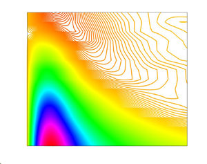
Figure 10 is an isocontour plot of the azimuthal velocity correlation $R_{u_{{1}}u_{{1}}}({{{\Delta }}}{s})$ for the four Reynolds numbers reported earlier at the wall-normal locations $0.1\le {{x_{{2}}/R}}\le {0.7}$. The figure allows better visualization for the effect of the Reynolds number on $R_{u_{{1}}u_{{1}}}({{{\Delta }}}{s})$ across the pipe versus the azimuthal separations $({{{\Delta }}}{s})$ for the wall-normal locations reported in figure 9. Due to axisymmetry of the pipe flow, it is worth noting that the data presented in figure 10 are for $0^{{\circ }}\le {{\Delta }}{\theta }\le {180^{{\circ }}}$ and imaged to the second half of the pipe cross-section. The contours and the colour levels in all plots are similar, i.e. the colour indicates the magnitude of $R_{u_{{1}}u_{{1}}}({{{\Delta }}}{s})$ given by the scale at the right of the plot. Qualitatively, the overall views of all four plots are similar; however, with deeper insight one can observe differences among all four plots, indicating a Reynolds number dependence, in disagreement with Bailey et al. (Reference Bailey, Hultmark, Smits and Schultz2008), who reported Reynolds number independence for the correlation coefficient. Figure 10 is believed to be more illustrative, indicating slight dependence of the two-point velocity correlation on the Reynolds number, the wall-normal distance and the azimuthal separation.

To better highlight the Reynolds number effects at various wall-normal locations, the cross-power spectral analysis is introduced in the next subsection. It might be noted, however, that slightly positive correlation values observed in figure 10 at large azimuthal separation and low Reynolds number would reflect possible flow periodicity in agreement with the conclusion made by Bailey et al. (Reference Bailey, Hultmark, Smits and Schultz2008). More analysis to quantify the sizes of the azimuthal scales of the LSMs for the present Reynolds number range $4100\le {{Re_{\tau }}}\le {15\,300}$ and the wall-normal distances $0.1\le {x_2/R}\le {0.7}$ is discussed in the following subsection.

3.3. Cross-power spectral density

In principle, the cross-correlation and cross-power spectral density functions are pairs of Fourier transforms. For specific purposes, one form is often preferred over the other, for instance, when the contribution of the LSMs and VLSMs to the azimuthal scale structures is to be evaluated. The velocity cross-correlation ${R_{u_{{1}}u_{{1}}}}({{{\Delta }}}{s})$ data illustrated in both figures 9 and 10 were estimated using (1.1), which was defined based on ensemble averaging of the hot-wire data, comprising contributions from a broad band of turbulence scales that mix the contributions of all wavenumbers to the azimuthal pipe LSMs. It was concluded by Bailey et al. (Reference Bailey, Hultmark, Smits and Schultz2008) that the averaging introduced in (1.1) obscures the proper contributions of both the LSMs and the VLSMs to the azimuthal scales. Thus the cross-power spectral density $G({{{\Delta }}}{s},k_{x_{{1}}})$ for the streamwise velocity fluctuations as a function of the azimuthal separation ${{{\Delta }}}{s}$ and the streamwise wavenumber $k_{x_{{1}}}$ was proposed (Bailey et al. Reference Bailey, Hultmark, Smits and Schultz2008), to overcome the averaging introduced in (1.1). The cross-power spectral density ${G}({{{\Delta }}}{s},k_{x_{{1}}})$ is defined as

(3.2)\begin{equation} {G}({{{\Delta}}}{s},k_{x_{{1}}})=F^*(0,k_{x_{{1}}})\,F({{{\Delta}}}{s},k_{x_{{1}}}), \end{equation}

where ${{G}({{{\Delta }}}{s},k_{x_{{1}}})}$ is calculated using Welch's averaging method, i.e. a modified periodogram method of spectral estimation. It is the fast Fourier transform of the cross-correlation function between the two signals recorded by the two hot-wire probes, simultaneously, each of sampling size indicated in table 1. It is worth noting that the cross-power spectral density is single-sided, yielding information about the power/energy shared over a range of wavenumbers as well as the coherence or the phase difference between the two signals received from the two hot-wire probes. It is therefore used to specify the power/energy shared at specific flow wavenumbers, for instance, corresponding to the LSM and the VLSM of the streamwise velocity fluctuations. The quantity $F^*(0,k_{x_{{1}}})$ is a complex conjugate of the finite Fourier transform of the streamwise velocity fluctuations ${u_{{1}}(0,t)}$ measured by the fixed radial probe, while $F({{{\Delta }}}{s},k_{x_{{1}}})$ is the finite Fourier transform of the streamwise velocity fluctuations ${u_{{1}}({{{\Delta }}}{s},t)}$ measured by the traversing azimuthal probe. The real component ${\varPsi }({{{\Delta }}}{s},k_{x_{{1}}})$ of the cross-power spectral density $G({{{\Delta }}}{s},k_{x_{{1}}})$, defined as

(3.3)\begin{equation} {\varPsi}({{{\Delta}}}{s},k_{x_{{1}}})={\rm Re}[G({{{\Delta}}}{s},k_{x_{{1}}})]\,{\sqrt{\langle{u_{{1}}^2(0,t)}\rangle}\,\sqrt{\langle{u_{{1}}^2({{{\Delta}}}{s},t)}}\rangle}, \end{equation}

is extracted and used to discuss further the distribution of the correlation of the streamwise velocity fluctuations as a function of the azimuthal separation ${{{\Delta }}}{s}$ and the streamwise wavenumber $k_{x_{{1}}}$ for various Reynolds numbers and wall-normal locations. On the other hand, the imaginary part of the cross-power spectral density function indicates whether the signals received from the two hot-wire probes are in phase or not. If both signals are in phase, then the cross-power spectral density is positive, while if they are ${\pm }{180^{\circ }}$ out of phase, then the cross-power spectral density is negative.

Figures 11 and 12 represent in outer scaling the real component ${\varPsi }({{{\Delta }}}{s},k_{x_{{1}}})$ of the cross-power spectral density normalized using the streamwise wavenumber $k_{x_{{1}}}$, the pipe radius $R$ and the wall friction velocity $u_{\tau }$, resulting in the so-called premultiplied cross-power spectral density $k_{x_{{1}}}R\,{\varPsi }({{{\Delta }}}{s},k_{x_{{1}}})/u_{\tau }u_{\tau }\equiv {k_{x_{{1}}}R{\varPsi }_{u_{{1}}u_{{1}}}^{++}}$, versus the streamwise wavenumber $k_{x_{{1}}}$ normalized with the pipe radius $R$, i.e. $k_{x_{{1}}}R$. Both figures 11 and 12 reflect the effect of the Reynolds number and the wall-normal location, respectively, on premultiplied cross-power spectral density $k_{x_{{1}}}R{\varPsi }_{u_{{1}}u_{{1}}}^{++}$. At fixed wall-normal location $x_2/R=0.7$, figure 11 presents $k_{x_{{1}}}R{\varPsi }_{u_{{1}}u_{{1}}}^{++}$ versus $k_{x_{{1}}}R$ for various azimuthal separations $10^\circ \le {\Delta {\theta }\le {210^\circ }}$ and Reynolds numbers $4100\le {{Re_{\tau }}}\le {15\,300}$. The figure shows a dependence of the peak–trough values of $k_{x_{{1}}}R{\varPsi }_{u_{{1}}u_{{1}}}^{++}$ and consequently the azimuthal structures on the Reynolds number as well as on the azimuthal separation for a fixed wall-normal location ${x_{{2}}/R}=0.7$. Further, figure 12 illustrates $k_{x_{{1}}}R{\varPsi }_{u_{{1}}u_{{1}}}^{++}$ versus the normalized streamwise wavenumber $k_{x_{{1}}}R$ at four wall-normal locations $0.1\le {x_{{2}}/R}\le {0.7}$ for various azimuthal separations $10^\circ \le {\Delta {\theta }\le {210^\circ }}$ and selected Reynolds number ${Re_{\tau }}=4100$. In both figures, the decrease in plot-line thickness as well as the downward arrow on all subplots indicate the direction of increasing azimuthal separation $\Delta {\theta }$ between the two probes. Figure 12 indicates a peak–trough mode with comparable behaviour for the wall-normal locations ${x_{{2}}/R}=0.1, 0.2$. In all four plots, the peak of $k_{x_{{1}}}R{\varPsi }_{u_{{1}}u_{{1}}}^{++}$ attenuates with increasing the azimuthal separation ${{{\Delta }}}{\theta }$ between the two probes, and the rate of attenuation/decay is higher for the closest pipe wall-normal locations ${x_{{2}}/R}=0.1, 0.2$, where the hot-wire probes in both plots belong to the logarithmic layer. For similar Reynolds number $Re_{\tau }=4100$, the peak value of $k_{x_{{1}}}R{\varPsi }_{u_{{1}}u_{{1}}}^{++}$ attenuates quickly with increasing both the azimuthal separation ${{{\Delta }}}{\theta }$ and the wall-normal location $x_{{2}}/R$; in particular, see figures 12(a–c) for $0.1\le {x_{{2}}}/R\le {0.5}$ up to azimuthal separation $\Delta {\theta } \approx {45}^{\circ }$. Changes in trough/negative values are also observable versus both the wall-normal location and the azimuthal separations. Those observations would be considered good indications of the coherence weaknesses as the azimuthal separation and the wall-normal locations increase. For the low Reynolds number cases, the viscous effect, in particular, near the pipe wall play an important role, contrary to the higher Reynolds number cases. Such rapid decay observed in $(k_{x_{{1}}}R{\varPsi }_{u_{{1}}u_{{1}}}^{++})_{peak}$ might also be interpreted by the hairpin vortex model proposed by Theodorsen (Reference Theodorsen1952). On the contrary, figures 11(d) and 12(d) for ${x_{{2}}/R}=0.7$ showed slow decay rate in $(k_{x_{{1}}}R{\varPsi }_{u_{{1}}u_{{1}}}^{++})_{peak}$ versus the azimuthal separation $\Delta {\theta }$, which could be attributed to the relatively long lifetimes of the azimuthal vortices found predominantly in the core region compared to figures 11(a–c) and 12(a–c).

Figure 11. Effect of Reynolds number on premultiplied cross-power spectral density $k_{x_{{1}}}R{\varPsi }_{u_{{1}}u_{{1}}}^{++}$ at fixed wall-normal location ${x_{{2}}/R}=0.7$. The downward arrow indicates increasing azimuthal separation $\Delta {\theta }$ between the two hot-wire probes. Plots are for ${x_{{2}}/R}=0.7$ and (a) ${{Re_{\tau }}}=4100$, (b) ${{Re_{\tau }}}=7700$, (c) ${{Re_{\tau }}}=11\,500$, and (d) ${{Re_{\tau }}}=15\,300$.

Figure 12. Effect of wall-normal location ${x_{{2}}/R}$ on premultiplied cross-power spectral density $k_{x_{{1}}}R{\varPsi }_{u_{{1}}u_{{1}}}^{++}$ for constant Reynolds number ${{Re_{\tau }}}=4100$. The downward arrow indicates increasing azimuthal separation $\Delta {\theta }$. Plots are for ${{Re_{\tau }}}=4100$ and (a) $x_2/R=0.1$, (b) $x_2/R=0.2$, (c) $x_2/R=0.5$, and (d) $x_2/R=0.7$.

To further support the data presented in figures 11 and 12, figures 13 and 14 are produced. Both figures 13 and 14 depict in outer scaling the isocontours of the real-part of premultiplied cross-power spectral density $k_{x_{{1}}}R{\varPsi }_{u_{{1}}u_{{1}}}^{++}$ versus the streamwise wavenumber normalized $k_{x_{{1}}}R$. Figure 13 presents isocontours of $k_{x_{{1}}}R{\varPsi }_{u_{{1}}u_{{1}}}^{++}$ versus $k_{x_{{1}}}R$ at $x_2/R=0.7$ for $4100\le {{Re_{\tau }}}\le {15\,300}$ and $10^\circ \le {\Delta {\theta }\le {210^\circ }}$. Similar to figure 11, figure 13 shows a clear dependence of the peak of $k_{x_{{1}}}R{\varPsi }_{u_{{1}}u_{{1}}}^{++}$ on the Reynolds number as well as on the azimuthal separation for fixed wall-normal location. For the four wall-normal locations ${x_{{2}}/R}= 0.1, 0.2, 0.5, 0.7$, figures 14(a–d) were produced, representing isocontours of $k_{x_{{1}}}R{\varPsi }_{u_{{1}}u_{{1}}}^{++}$ for ${{Re_{\tau }}}=4100$. The figure allows, for the same Reynolds number, better visualization of the effect of changing the wall-normal position and the azimuthal separation on $k_{x_{{1}}}R{\varPsi }_{u_{{1}}u_{{1}}}^{++}$. One would, clearly, observe the regions of positive and negative values of $k_{x_{{1}}}R{\varPsi }_{u_{{1}}u_{{1}}}^{++}$ over various ranges of the azimuthal probe separation ${{{\Delta }}}{\theta }$. Mostly, the negatively correlated signals occur at low and moderate streamwise wavenumbers $k_{x_{{1}}}R$ – however, at large enough azimuthal probe separation. The positive–negative values of $k_{x_{{1}}}R{\varPsi }_{u_{{1}}u_{{1}}}^{++}$ shown in both figures 13 and 14 emphasize the contribution of the LSMs to the azimuthal coherent structure. One thus could deduce from figures 11–14 clear evidence for the dependence of the cross-power spectral density and consequently the azimuthal pipe flow structure on the Reynolds number, the wall-normal location for various azimuthal separations.

Figure 13. Isocontours of $k_{x_{{1}}}R{\varPsi }_{u_{{1}}u_{{1}}}^{++}$ at fixed wall-normal location ${x_{{2}}/R}=0.7$ and four Reynolds numbers: (a) ${Re_{\tau }}=4100$, (b) ${Re_{\tau }}=7700$, (c) ${Re_{\tau }}=11\,500$, and (d) ${Re_{\tau }}=15\,300$.

Figure 14. Isocontours of the real component of premultiplied cross-spectral density $k_{x_{{1}}}R{\varPsi }_{u_{{1}}u_{{1}}}^{++}$ at four wall-normal locations for Reynolds number ${{Re_{\tau }}}=4100$ and $10^{\circ }\le \Delta {\theta }\le {80^{\circ }}$: (a) ${x_{{2}}/R}=0.1$, (b) ${x_{{2}}/R}=0.2$, (c) ${x_{{2}}/R}=0.5$, and (d) ${x_{{2}}/R}=0.7$.

In figures 11–14, at each azimuthal separation within the range ${10^{\circ }}\le {\Delta {\theta }}\le {70^{\circ }}$, positive and negative values for $k_{x_{{1}}}R{\varPsi }_{u_{{1}}u_{{1}}}^{++}$ were obtained – however, along different ranges of the streamwise wavenumber $k_{x_{{1}}}R$. To investigate further the effect of changing the azimuthal separation ${\Delta {\theta }}$, the wall-normal location ${x_{{2}}/R}$ and the Reynolds number ${Re_{\tau }}$ on $k_{x_{{1}}}R{\varPsi }_{u_{{1}}u_{{1}}}^{++}$, figure 15 was produced. Figure 15 consists of four plots. Figure 15(a) is a zoomed version of figure 12(d) to highlight the positive–negative/peak–trough values of $k_{x_{{1}}}R{\varPsi }_{u_{{1}}u_{{1}}}^{++}$ versus $k_{x_{{1}}}R$ at ${x_{{2}}/R}=0.7$ for azimuthal separations ${10^{\circ }}\le {\Delta {\theta }}\le {210^{\circ }}$ and ${Re_{\tau }}=4100$. Furthermore, each plot in figures 12(a)–(c) is zoomed and treated in a similar manner to the zoomed version of figure 12(d), and the outcomes, i.e. both peak/positive and trough/negative values of $k_{x_{{1}}}R{\varPsi }_{u_{{1}}u_{{1}}}^{++}$, for all wall-normal locations $0.1\le {x_{{2}}/R}\le 0.7$ and ${Re_{\tau }}=4100$, are presented in figures 15(b,c). The effect of the wall-normal location ${x_{{2}}/R}$ on either the peak/positive and trough/negative values of $k_{x_{{1}}}R{\varPsi }_{u_{{1}}u_{{1}}}^{++}$ is observable in both figures 15(b,c) for the same Reynolds number. However, such peak/positive, trough/negative behaviour of $(k_{x_{{1}}}R{\varPsi }_{u_{{1}}u_{{1}}}^{++})_{peak\unicode{x2013}trough}$ is more prominent for the wall-normal locations ${x_{{2}}/R}\le {0.1}$ and ${x_{{2}}/R}\le {0.2}$, as figure 15(b) indicates. In figure 15(c), for similar azimuthal probe separation and constant Reynolds number, a strong effect for the wall-normal location on either the peak/positive or trough/negative values of $k_{x_{{1}}}R{\varPsi }_{u_{{1}}u_{{1}}}^{++}$ is observable, in particular for ${x_{{2}}/R}=0.1$ and 0.2. On the other hand, the peak values of $k_{x_{{1}}}R{\varPsi }_{u_{{1}}u_{{1}}}^{++}$ attenuate fast on moving away from the pipe wall, as both figures 15(b,c) illustrate. One would also observe from figure 15(c) that along an azimuthal separation range ${45^{\circ }}\le {\Delta {\theta }}\le {150^{\circ }}$, $k_{x_{{1}}}R{\varPsi }_{u_{{1}}u_{{1}}}^{++}$ shows almost zero values, indicating that the two hot-wire signals are uncorrelated along this azimuthal separation range. Additionally, figure 15(d) represents the effect of the Reynolds number within the range ${4100}\le {{Re_{\tau }}}\le {15\,300}$ on the peak–trough values of $k_{x_{{1}}}R{\varPsi }_{u_{{1}}u_{{1}}}^{++}$ at ${x_{{2}}/R}=0.7$ fixed wall-normal location. The figure shows a clear effect for the Reynolds number on peak/positive and/or trough/negative values of $k_{x_{{1}}}R{\varPsi }_{u_{{1}}u_{{1}}}^{++}$ at similar azimuthal separation $\Delta {\theta }$. Therefore, one would conclude that figure 15 is clear evidence for the dependence of the azimuthal scale structure of the LSMs on the azimuthal separation $\Delta {\theta }$, the wall-normal location ${x_{{2}}/R}$ and the Reynolds number ${Re_{\tau }}$.

Figure 15. Peak–trough behaviour of the real component of premultiplied cross-power spectral density $k_{x_{{1}}}R{\varPsi }_{u_{{1}}u_{{1}}}^{++}=f(\Delta {\theta },{x_{{2}}/R},{Re_{\tau }})$: (a) zoomed $k_{x_{{1}}}R{\varPsi }_{u_{{1}}u_{{1}}}^{++}$ versus $k_{x_{{1}}}R$; (b) $(k_{x_{{1}}}R{\varPsi }_{u_{{1}}u_{{1}}}^{++})_{peak\unicode{x2013}trough}$ versus ${x_{{2}}/R}$; (c) $(k_{x_{{1}}}R{\varPsi }_{u_{{1}}u_{{1}}}^{++})_{peak\unicode{x2013}trough}$ versus $\Delta {\theta }$ for $0.1\le {x_{{2}}/R}\le {0.7}$; (d) $(k_{x_{{1}}}R{\varPsi }_{u_{{1}}u_{{1}}}^{++})_{peak\unicode{x2013}trough}$ versus $\Delta {\theta }$ for $4.1\times {10^3}\le {{Re_{\tau }}}\le {15.3\times {10^3}}$. Plots are for (a) ${Re_{\tau }}=4100$ and ${x_{{2}}/R}=0.7$, (b) ${Re_{\tau }}=4100$ and ${10^{\circ }}\le {\Delta {\theta }}\le {210^{\circ }}$, (c) ${Re_{\tau }}=4100$ and $0.1\le {x_{{2}}/R}\le {0.7}$, and (d) $4100\le {{Re_{\tau }}}\le {15\,300}$ and ${x_{{2}}/R}={0.7}$.

To assess quantitatively the fractional contribution of the large-scale motions, i.e. VLSM and LSM, to the azimuthal pipe flow structure, a spectral filtration for the cross-power spectral density was performed; see Bailey et al. (Reference Bailey, Hultmark, Smits and Schultz2008). The contribution of the VLSM was made via

(3.4)\begin{equation} {\rho}_{{VL}}({{{\Delta}}}{s},{k_{{x}_{{1}}}})= \int_{0}^{({{k_{{x}_{{1}}}}})_{cut}}{{\rm Re}[G({{{\Delta}}}{s},{k_{{x}_{{1}}}})]\,{\rm d}{k_{{x}_{{1}}}}}, \end{equation}

where $({{k_{x_{1}}})_{cut}}$ is the streamwise wavenumber corresponding to the first peak appearing in the premultiplied power spectra presented in both figures 7 and 8, and it depends on the wall-normal location and Reynolds number. Thus the contribution of the VLSMs to the pipe flow azimuthal structure was evaluated for ${{k_{x_{{1}}}}}\le {{(k_{x_{{1}}}})_{cut}}$. On the other hand, the contribution of the LSMs is examined for ${{k_{x_{{1}}}}}\ge {{(k_{x_{{1}}}})_{cut}}$ using

(3.5)\begin{equation} {\rho}_{L}({{{\Delta}}}{s},{k}_{x_{{1}}})= \int_{{(k_{x_{{1}}})}_{cut}}^{\infty}{{\rm Re}[G({{{\Delta}}}{s},{k}_{x_{{1}}})]\,{\rm d}{k}_{x_{{1}}}}. \end{equation}

The azimuthal distribution of both $\rho _{{VL}}({{{\Delta }}}{s},{k_{{x}_{{1}}}})$ and $\rho _{L}({{{\Delta }}}{s},{k_{{x}_{{1}}}})$ for ${{k_{x_{{1}}}}}\le {{(k_{x_{{1}}}})_{cut}}$ and ${{k_{x_{{1}}}}}\ge {{(k_{x_{{1}}}})_{cut}}$, respectively, are presented in figure 16 for $0.1\le {{x_{{2}}/R}}\le {0.7}$ and ${{Re_{\tau }}}=7700$, and compared to the azimuthal distribution of the streamwise velocity correlation ${R_{u_{{1}}u_{{1}}}({{{\Delta }}}{s}})$. For similar Reynolds numbers, a clear dependence of both $\rho _{VL}({{{\Delta }}}{s},k_{x_{{1}}})$ and $\rho _{L}({{{\Delta }}}{s},k_{x_{{1}}})$ on the azimuthal separation ${{{\Delta }}}{s}$ and the wall-normal location $x_{{2}}$ is observable. For small azimuthal separation ${{{\Delta }}}{s}/R\le {1}$, one would observe agreement with Bailey et al. (Reference Bailey, Hultmark, Smits and Schultz2008), but with the discernible difference that the magnitude of $\rho _{VL}({{{\Delta }}}{s},k_{x_{{1}}})$ is greater than that of $\rho _{L}({{{\Delta }}}{s},k_{x_{{1}}})$, reflecting an increased contribution of the VLSM to the azimuthal pipe flow structures. This observation is also a good indication that the azimuthal scales vary with the wall-normal location as well as with the azimuthal separation. Figure 16 stresses the effect of scale averaging when using (1.1) compared to the azimuthal scales estimated based on both (3.4) and (3.5), addressing the contributions of the large-scale motions, i.e. VLSM and LSM, respectively, as will be shown later, in figure 19. However, one might observe from figure 16 changes in the magnitude and ranges of the negative values of both $\rho _{{VL}}({{{\Delta }}}{s},k_{x_{{1}}})$ and $\rho _{L}({{{\Delta }}}{s},k_{x_{{1}}})$ versus the wall-normal distance for fixed Reynolds number. Referring to figure 7(a) for ${x_{{2}}/R}=0.1$, where the VLSM is more energetic than the LSM, the VLSM contributes more to the azimuthal correlation coefficient, as figure 16(a) indicates. The contribution of the VLSM decreases, however, on moving away from the pipe wall, and on reaching ${x_{{2}}/R}=0.5$, one would observe, as figure 7(c) indicated, that the energy contained in the LSM is larger relative to that contained in the VLSM, reflecting changes in the contribution of the LSM to the azimuthal correlation coefficient $\rho _{L}({{{\Delta }}}{s},k_{x_{{1}}})$ when compared to the contribution of the VLSM, as figure 16 illustrates.

Figure 16. Azimuthal distributions of $\rho _{VL}({{{\Delta }}}{s},k_{x_{{1}}})$ and $\rho _{{L}}({{{\Delta }}}{s},k_{x_{{1}}})$ for (a) ${x_{{2}}/R}= 0.1$, (b) ${x_{{2}}/R}=0.2$, (c) ${x_{{2}}/R}= 0.5$ and (d) ${x_{{2}}/R}= 0.7$, for Reynolds number ${{Re_{\tau }}}=7700$.

3.4. Coherence function

To investigate further the behaviour of the azimuthal large scales at some specific wavenumbers in correspondence with the VLSM and LSM, the coherence function is introduced. It is a measure of the correlation between the two streamwise velocity fluctuating signals received from both probes, but in terms of the energy contained at specific wavenumbers. Bendat & Piersol (Reference Bendat and Piersol2000) introduced the so-called magnitude-squared coherence or the coherence function, defined as

(3.6)\begin{equation} \gamma^2({{{\Delta}}}{s},k_{x_{{1}}})=\frac{|{{\varPsi({{{{\Delta}}}{s},k_{x_{{1}}})}}}|^2}{{\varPhi({{{0}},k_{x_{{1}}}}})\,{{\varPhi({{{{\Delta}}}{s},k_{x_{{1}}})}}}}. \end{equation}

This definition of the coherence function results in loss of its negative values, which have potential to assess the azimuthal scales of the coherent structures. Thus, in alignment with Bailey et al. (Reference Bailey, Hultmark, Smits and Schultz2008), we adopted the following definition of the coherence function:

(3.7)\begin{equation} \gamma({{{\Delta}}}{s},k_{x_{{1}}})=\frac{{{\varPsi({{{{\Delta}}}{s},k_{x_{{1}}})}}}}{{\varPhi^{{1/2}}({{{0}},k_{x_{{1}}}}})\,{{\varPhi^{{1/2}}({{{{\Delta}}}{s},k_{x_{{1}}})}}}}, \end{equation}

quantifying the differences in the behaviour of the azimuthal scales as a result of the VLSM and LSM, where ${\varPsi ({{{{\Delta }}}{s},k_{x_{{1}}})}}$ as defined earlier is the real component of the cross-power spectral density ${G}({{{\Delta }}}{s},k_{x_{{1}}})$, ${\varPhi ({{0}},k_{x_{{1}}})}$ is the auto-spectral density of the streamwise velocity fluctuations received from the fixed radial hot-wire probe, and ${\varPhi ({{{{\Delta }}}{s},k_{x_{{1}}})}}$ is the auto-spectral density of the streamwise velocity fluctuations measured by the traversing azimuthal probe.

It was shown earlier in power spectra presented in both figures 7 and 8 that two specific wavenumbers related to the VLSMs and LSMs were determined. Hence the coherence function $\gamma ({{{\Delta }}}{s},k_{x_{{1}}})$ should be computed at such corresponding wavenumbers. In spite of the fact that the coherence function and the spectral density functions are pairs of the Fourier transform, the coherence function is more convenient for evaluating the azimuthal scales of the LSMs; see Bailey et al. (Reference Bailey, Hultmark, Smits and Schultz2008) and Bendat & Piersol (Reference Bendat and Piersol2000). Figure 17 represents the azimuthal distribution of $\gamma ({{{\Delta }}}{s},k_{x_{{1}}})$ estimated at the streamwise wavenumbers corresponding to both the VLSM and the LSM at four wall-normal locations for ${Re_{\tau }}=4100$. At first glance, one concludes that the distribution of $\gamma ({{{\Delta }}}{s},k_{x_{{1}}})$ is similar to those of $R_{u_{{1}}u_{{1}}}({{{\Delta }}}{s})$ shown earlier in both figures 9 and 10. It is observable from figure 17, however, that at the same azimuthal separation ${{\Delta }}{s/R}$, the magnitude of $\gamma ({{{\Delta }}}{s},k_{x_{{1}}})$ has higher negative values than those for $R_{u_{{1}}u_{{1}}}({{{\Delta }}}{s})$, reflecting the effect of the ensemble averaging of the various scales of flow motions introduced in the traditional definition of the streamwise velocity correlation $R_{u_{{1}}u_{{1}}}({{\Delta }}{s})$. On the contrary, the effect of the averaging in $\gamma ({{{\Delta }}}{s},k_{x_{{1}}})$ is limited to two main wavelengths corresponding to the two-mode peaks observed in both figures 7 and 8 identifying the VLSM and LSMs.

Figure 17. Azimuthal coherence function $\gamma ({{{\Delta }}}{s},k_{x_{{1}}})$ based on streamwise wavenumbers corresponding to LSMs and VLSMs at four wall-normal locations for Reynolds number ${{Re_{\tau }}}=4100$: (a) $x_2/R=0.1$, (b) $x_2/R=0.2$, (c) $x_2/R=0.5$, and (d) $x_2/R=0.7$.

To quantify the azimuthal length scale ($\ell _z^+$) of the LSMs, selected samples of the streamwise velocity correlation $R_{u_{{1}}u_{{1}}}({{{\Delta }}}{s})$ for ${Re_{\tau }}=4100$ and $7700$ are presented versus the azimuthal probe separation in wall units ${{{\Delta }}}{s^+}$ in figure 18, where ${{{\Delta }}}{{s}^+}={{{\Delta }}}{s}\,u_{\tau }/\nu$. The $R_{u_{{1}}u_{{1}}}({{{\Delta }}}{s})$ correlation drops from 1 to negative values at a range of azimuthal displacement ${{{\Delta }}}{s}^+\approx {100\unicode{x2013}5500}$ wall units, depending on the Reynolds number. Both plots in figure 18 show a similar trend where the value of $R_{u_{{1}}u_{{1}}}({{{\Delta }}}{s})$ drops to negative values, indicating the occurrence of alternating high-speed and low-speed regions of velocity fluctuations in the azimuthal direction. A threshold 0.05 is proposed in figure 18 to estimate the azimuthal length scale ($\ell _z^+$) of the LSMs based on $R_{u_{{1}}u_{{1}}}({{{\Delta }}}{s})$. In a similar manner, the azimuthal length scale is thus computed across the whole range of the wall-normal locations, i.e. $0.1\le {{x_{{2}}/R}}\le {0.7}$, and Reynolds numbers $4100\le {Re_{\tau }}\le {15\,300}$, and the results are illustrated in figures 19(a,b). The results indicate that typical azimuthal scales of the large flow structures increase in diameter with increase in the wall-normal distance, in qualitative agreement with a similar observation made by Ganapathisubramani et al. (Reference Ganapathisubramani, Hutchins, Hambleton, Longgmire and Marusic2005) for flat-plate boundary layer flow. The figure shows linear behaviour of the azimuthal growth of the large-scale structures across the logarithmic layer, in close agreement with Tomkins & Adrian (Reference Tomkins and Adrian2003), Monty et al. (Reference Monty, Stewart, Williams and Chong2007) and Bailey et al. (Reference Bailey, Hultmark, Smits and Schultz2008). On the other hand, a nonlinear increase versus the wall distance through the core region, i.e. ${x_{{2}}/R}\ge {0.5}$, is remarkable. Focusing more on the $\ell _z/R$ data trend in figure 19(a), it does indeed appear nonlinear/concave-up, whereas in figure 9(a) of Bailey et al. (Reference Bailey, Hultmark, Smits and Schultz2008), the $\ell _z/\delta$ results from a couple of experiments seem quite linear, modestly far from the wall – however, overall concave-down. It is worth noting here that most of the earlier azimuthal studies did not cover either the core region of the pipe flow or the outer region of the boundary layer, thus the nonlinear behaviour of the azimuthal structure was not discovered. For instance, using high spatial resolution particle image velocimetry, Tomkins & Adrian (Reference Tomkins and Adrian2003) reported that several spanwise length scales vary, remarkably, linearly along the logarithmic layer in support of the attached-eddy hypothesis (Townsend Reference Townsend1956). Note that measurements of Tomkins & Adrian (Reference Tomkins and Adrian2003) were limited to the wall-normal distances $x_2/\delta \le {0.2}$. The discrepancy observed between the present finding versus the literature might be attributed partially to unequal ranges of the wall-normal distances and the Reynolds numbers. The uncertainty in calibration equations and spatial resolutions of the hot-wire probes to resolve small-scale turbulent fluctuations also has to be taken into consideration.

Figure 18. The azimuthal velocity correlation $R_{u_{{1}}u_{{1}}}({{{\Delta }}}{s})$ of the streamwise velocity fluctuations at four wall-normal locations $0.1\le {{x_{{2}}/R}}\le {0.7}$ versus the azimuthal displacement in wall units ${{\Delta }}{s}^+$: (a) ${Re}_{\tau }=4100$, (b) ${Re}_{\tau }=7700$.

Figure 19. Normalized azimuthal length scale $\ell _z/R$ of azimuthal LSMs based on velocity correlations of the streamwise velocity fluctuations (a) compared to $\gamma _{_{L}}({{{\Delta }}}{s},k_{x_{{1}}})$ and $\gamma _{_{VL}}({{{\Delta }}}{s},k_{x_{{1}}})$ (present data), and (b) locally scaled by $2{\rm \pi} {r}$ and compared to Bailey et al. (Reference Bailey, Hultmark, Smits and Schultz2008) (${Re_b}=7.6\times {10^4}\text { and } 8.3\times {10^6}$).

Moreover, Bailey et al. (Reference Bailey, Hultmark, Smits and Schultz2008) claimed that the azimuthal length scale $\ell _z$ variation versus the wall-normal location $x_2$ is completely linear when scaled appropriately by the local circumference ($2{\rm \pi} {r}$) at a given height to account for the pipe geometry. Note that the Bailey et al. (Reference Bailey, Hultmark, Smits and Schultz2008) data were limited to the wall-normal distances $0.1\le {x_2/R}\le {0.5}$. The current pipe data for $0.1\le {x_2/R}\le {0.7}$ are examined in a similar manner to Bailey et al. (Reference Bailey, Hultmark, Smits and Schultz2008) and plotted in figure 19(b). The present $\ell _z/(2 {\rm \pi}r)$ data showed very strong deviation from linearity in the core region of the pipe, i.e. for the final measurement location at $x_2/R = 0.7$, in which case this would constitute a significant deviation from Tomkins & Adrian (Reference Tomkins and Adrian2003), Monty et al. (Reference Monty, Stewart, Williams and Chong2007) and Bailey et al. (Reference Bailey, Hultmark, Smits and Schultz2008). Figure 19(b) might support the idea that the nonlinearity is not a result of the pipe geometry alone (Townsend Reference Townsend1956), as Bailey et al. (Reference Bailey, Hultmark, Smits and Schultz2008) suggested. The nonlinear behaviour observed in the present study is beyond the top of the logarithmic layer, i.e. in the core region of the pipe where the attached-eddy hypothesis deviates. However, the significant difference in the wall-normal behaviours of the azimuthal scales of the observed LSM and VLSM is in alignment with a conclusion made by Bailey et al. (Reference Bailey, Hultmark, Smits and Schultz2008) that the LSM and VLSM are independent entities.

3.5. Streamwise large-scale structure

Intensive efforts have been recognized – see e.g. Theodorsen (Reference Theodorsen1952), Townsend (Reference Townsend1956), Grant (Reference Grant1958), Lumley (Reference Lumley1967), Sabot et al. (Reference Sabot, Renault and Comte-Bellot1973), Cantwell (Reference Cantwell1981), Hussain (Reference Hussain1983,  Reference Hussain1986), Robinson (Reference Robinson1991), Wark & Nagib (Reference Wark and Nagib1991), Kim & Adrian (Reference Kim and Adrian1999), Tomkins & Adrian (Reference Tomkins and Adrian2003), Morrison (Reference Morrison2007), Monty et al. (Reference Monty, Stewart, Williams and Chong2007), Marusic et al. (Reference Marusic, McKeon, Monkewitz, Nagib, Smits and Sreenivasan2010), Smits et al. (Reference Smits, Monty, HUltmark, Bailey, Hutchins and Marusic2011b), Chung et al. (Reference Chung, Marusic, Monty, Vallikivi and Smits2015), Baidya et al. (Reference Baidya2019) and Zanoun et al. (Reference Zanoun, Öngüner, Egbers, Bellani and Talamelli2019) – addressing questions often raised in the literature concerning the large-scale structures in wall-bounded shear flows. Nevertheless, a concrete definition of the origin, nature and time evolution of such structures is still under debate (see e.g. Marusic et al. Reference Marusic, McKeon, Monkewitz, Nagib, Smits and Sreenivasan2010; Jiménez Reference Jiménez2018), motivating further investigations to characterize, appropriately, the large-scale structures, in particular at high Reynolds numbers. For instance, a number of scenarios have been proposed by Panton (Reference Panton2001), characterizing mechanisms for the sustenance of wall turbulence which related to the turbulence structures of wall-bounded shear flows. They have been classified recently by Marusic et al. (Reference Marusic, McKeon, Monkewitz, Nagib, Smits and Sreenivasan2010) into two broad classes: one class is based on instability and transient growth mechanisms principally in the inner region, and the other is based on vortex-structure regeneration mechanisms. In alignment with the view of Marusic et al. (Reference Marusic, McKeon, Monkewitz, Nagib, Smits and Sreenivasan2010), Del Álamo & Jiménez (Reference Del Álamo and Jiménez2006) suggested that the LSMs might arise from nonlinear instabilities in pipe flow turbulence. However, the interpretation of the LSMs in most earlier studies agreed with the hairpin vortex paradigm of Theodorsen (Reference Theodorsen1952). Thus the hairpin concept might be considered a universal element or a building block of the large-scale structure of turbulent flow as proposed by Theodorsen (Reference Theodorsen1952) and later adopted by Kim & Adrian (Reference Kim and Adrian1999) and Adrian (Reference Adrian2007). And adopting the conceptual model by Kim & Adrian (Reference Kim and Adrian1999), the very-large-scale structure was defined as a consequence of coherence in the pattern of hairpin packets, i.e. the hairpin eddies that align coherently in groups to form long packets, and then packets align coherently to form the VLSMs.

In the present work, to highlight the sizes of the LSMs in the streamwise direction, intensive measurements using a single hot-wire probe were carried out, covering the inner and core regions of the pipe, i.e. ${0.04}\le {{x_{{2}}/R}}\le {1}$, through multiple radial locations. The analysis of the spectra shown earlier in both figures 7 and 8 proposed two-mode structures, i.e. a low-wavenumber mode and a moderate-wavenumber mode.

Further data analysis was therefore carried out, allowing estimations of the streamwise sizes of the large-scale structures, and the outcome is presented in figure 20. Figure 20 illustrates for different Reynolds numbers the values of the wavelengths $\lambda _{max}/R$ of the two-mode flow structures versus the wall-normal location $x_2/R$, both normalized by the pipe radius $R$. Although the validity of Taylor's hypothesis to convert temporal hot-wire signals into spatial domain data remains a big concern (see e.g. Zaman & Hussain Reference Zaman and Hussain1981; Marusic et al. Reference Marusic, McKeon, Monkewitz, Nagib, Smits and Sreenivasan2010), it was used in the present study to estimate the sizes of the streamwise large-scale structures. Thus, based on similar analysis for the spectral peaks observed in figures 7 and 8, the sizes of the large-scale structures were estimated using the Taylor hypothesis discussed in § 3.1, and the results are presented in figure 20. Briefly, the indices/wavenumbers at which the first and second local maxima/peaks of the energy spectra occur are determined in correspondence with the VLSMs and LSMs, respectively. Thereafter, the wavelengths ${\lambda _{x_{{1}}}}={2{\rm \pi} }/{{k_{x_{{1}}}}}$ associated with the low and moderate wavenumbers for the very-large-scale and large-scale structures were estimated and then normalized with the pipe radius ${\lambda _{x_{{1}}}}/R$, respectively. In figure 20, it is observed that the wavelengths of those structures change significantly along the pipe wall-normal distance as well as with the Reynolds number. Figure 20(a) is a semi-logarithmic representation of the large-scale structures. Thus one might observe slight differences between the LSMs and VLSMs within the buffer layer. The figure illustrates also that the very-large-scale structures start roughly at the top of the buffer layer, in agreement with a similar conclusion made by Kim & Adrian (Reference Kim and Adrian1999), and grow rapidly in wavelength $\lambda _{x_{{1}}}$ through the logarithmic region, reaching maximum wavelengths $\lambda _x\approx {12}R$, $\lambda _x\approx {16}R$ and $\lambda _{x_{{1}}}\approx {18}R$ for ${Re_{\tau }}=3200$, ${Re_{\tau }}=11\,000$ nd ${Re_{\tau }}\approx 16\,000$, respectively, at approximately half of the pipe radius ${x_{{2}}/R}\approx {0.5}$, i.e. outside the logarithmic layer. A sudden drop in the wavelength of the VLSM occurs at ${x_{{2}}/R}\approx {0.5}$, which is also in alignment with an observation made by Meinhart & Adrian (Reference Meinhart and Adrian1995) and Kim & Adrian (Reference Kim and Adrian1999) that the VLSMs are associated with the zones of uniform low momentum found in the boundary layer, which extend only up to approximately one-half of the boundary layer thickness or the pipe radius. Figure 20(b) is a linear plot, better showing the LSM along the core region of the pipe. One structure beyond $x_2/R=0.5$, having wavelength $\lambda _x\approx {3R}$, is observable. Hence one concludes from figures 20(a,b) that the LSM spans the pipe cross-section from a location close to the pipe wall, i.e. within the buffer layer, to the centreline of the pipe, having wavelength $\lambda _{x}$ around $3R$ in plausible agreement also with Kim & Adrian (Reference Kim and Adrian1999). The constant behaviour of the LSM along the buffer and the logarithmic layers might be attributed to the attached-eddy model of wall turbulence; see e.g. Marusic & Monty (Reference Marusic and Monty2019).

Figure 20. (a) Semi-logarithmic and (b) linear representations of the dimensionless wavelengths of the LSMs and VLSMs versus the normalized wall-normal distances for ${2150}\le {{Re}_{\tau }}\le {16\times {10^3}}$.