


1. Introduction
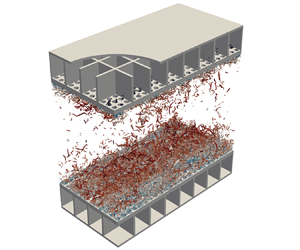
Aircraft engines are the primary source of noise during take-off and landing. In order to meet noise regulations, the nacelle of modern engines is coated with acoustic liners, which represent the state-of-the-art technology for engine noise abatement. Acoustic liners are panels with a sandwich structure, consisting of a honeycomb core, bounded by a perforated facesheet and a solid backplate (see figure 1a). They cover the nacelle inner surface, both in front of the fan and in the by-pass duct (see figure 2), and can theoretically absorb all incoming sound if the resonant frequency of the liner is tuned to the frequency of the incoming acoustic wave (Hughes & Dowling Reference Hughes and Dowling1990; Dowling & Hughes Reference Dowling and Hughes1992; Kirby & Cummings Reference Kirby and Cummings1998). In realistic conditions, several studies have shown that acoustic liners reduce fan noise by as much as 3–6 dB (Casalino, Hazir & Mann Reference Casalino, Hazir and Mann2018; Shur et al. Reference Shur, Strelets, Travin, Suzuki and Spalart2020). They are, therefore, an essential part of aircraft engines.
(a) Turbofan engine of a civil aircraft with acoustic liners on the air intake. (b) The typical pore size of acoustic liners used in turbofan engines.

Acoustic liners around the fan of a turbofan engine.

Although the sound attenuation mechanism is well understood, the aerodynamic characteristics of these surfaces are less clear. Several authors agree that liners increase aerodynamic drag as compared with a hydraulically smooth wall (Wilkinson Reference Wilkinson1983; Howerton & Jones Reference Howerton and Jones2015; Jasinski & Corke Reference Jasinski and Corke2020). However, an extensive literature study summarized in table 1 shows that reported values for the actual drag increase caused by acoustic liners vary between 2 % and 500 %. Hence, at present, we lack a theory for the prediction of the aerodynamic drag over acoustic liners.
Dataset of previous studies of drag over acoustic liner geometries. Here  $M_{\infty }$ is the Mach number, $\textit {Re}_{\delta }=u_0\delta /\nu$ is the Reynolds number based on the boundary layer thickness and external velocity (free-stream velocity for boundary layers or bulk flow velocity for channel flow simulations) and $\textit {Re}_\tau$ is the friction Reynolds number. The liner geometry is defined by the orifice diameter $d$, the depth of the cavity $h$, the thickness of the facesheet $t$ and the porosity $\sigma$. Parameter $\Delta D$ is the percentage increase in drag observed in these studies. Quantities that are approximated are denoted using the $^{{\dagger} }$ superscript. Quantities that are approximated using Reynolds-averaged Navier–Stokes simulations of the GFIT by Zhang & Bodony (Reference Zhang and Bodony2016) are denoted using the $^{\circledast }$ superscript.

Wilkinson (Reference Wilkinson1983) was among the first to perform experiments of turbulent boundary layers over porous plates for different values of the viscous-scaled orifice diameter  $d^+\unicode{x2254} d/\delta _v$, viscous-scaled plate thickness $t^+\unicode{x2254} t/\delta _v$ and plate porosity (open-area ratio) $\sigma$. Here, $\delta _v=\nu _w/u_\tau$ is the viscous length scale, $\nu$ the kinematic viscosity of the fluid, $u_\tau =\sqrt {\tau _w/\rho _w}$ the friction velocity, $\tau _w$ the drag per plane area and $\rho$ the fluid density and the subscript $w$ denotes quantities evaluated at the wall.
More recently, several experiments have been conducted in the Grazing Flow Impedance Tube (GFIT) facility at NASA (Jones et al. Reference Jones, Watson, Parrott and Smith2004a) and considerable effort has been dedicated to estimating the added drag provided by acoustic liners using a static pressure drop approach (Howerton & Jones Reference Howerton and Jones2015, Reference Howerton and Jones2016, Reference Howerton and Jones2017). These experimental campaigns considered several liner geometries, for both conventional and more exotic configurations (Howerton & Jones Reference Howerton and Jones2015, Reference Howerton and Jones2017), and reported a drag increase of between 16 % and 350 % compared with a smooth wall.
An important finding of the GFIT experiments is that the cavity depth has a negligible contribution to the total drag in the absence of acoustic waves, which instead is largely influenced by the orifice diameter, plate porosity and facesheet thickness. For instance, Howerton & Jones (Reference Howerton and Jones2015) noted that, for constant porosity, reducing the diameter of the orifices reduced drag. Similarly, Howerton & Jones (Reference Howerton and Jones2017) reported 50 % drag increase for porosity  $\sigma =0.08$ and 400 % drag increase for $\sigma =0.3$, for the same flow conditions and approximately the same orifice diameter. Additionally, these experiments suggest that it is possible to reduce the drag penalty without harming the noise attenuation.
Gustavsson et al. (Reference Gustavsson, Zhang, Cattafesta and Kreitzman2019) performed experiments over several acoustic liner geometries and reported a drag increase of between 30 % and 50 %, without incoming acoustic waves, arguing that the added drag might be even larger in the presence of incoming noise.
Numerical simulations of turbulent flows over acoustic liners are also available, but very often they rely on simplified configurations or wall models because pore-resolved simulations are computationally expensive. A common approach that has been pursued for reducing the computational cost is to simulate a single cavity rather than an array of resonators (Zhang & Bodony Reference Zhang and Bodony2011, Reference Zhang and Bodony2016; Avallone et al. Reference Avallone, Manjunath, Ragni and Casalino2019). Zhang & Bodony (Reference Zhang and Bodony2016) performed direct numerical simulation (DNS) of turbulent grazing flow over a single resonator with a cavity geometry similar to that studied by Howerton & Jones (Reference Howerton and Jones2015) in the GFIT (Jones et al. Reference Jones, Watson, Tracy and Parrott2004b). However, the simulations were at a much lower friction Reynolds number (see table 1). For a free-stream Mach number  $M_\infty =0.5$, Zhang & Bodony (Reference Zhang and Bodony2016) reported a minor drag increase of $4.2\,\%$ with respect to a smooth wall in the absence of sound waves, whereas they found a drag increase of about 25 % when including sound waves with an intensity of 140 dB. These results seem to contradict experiments of Howerton & Jones (Reference Howerton and Jones2015) who reported a drag increase of about 50 % both with and without incoming sound waves, at matched Mach number and cavity geometry. This discrepancy can probably be traced back to the simplified numerical set-up wherein only one single orifice is simulated, resulting in a very low porosity $\sigma =0.0099$, compared with $\sigma =0.08$ in the experiments.
Another common simplification in numerical simulation is to approximate the effect of acoustic liners with an equivalent impedance boundary condition (Tam & Auriault Reference Tam and Auriault1996), which substantially reduces the computational cost. However, the accuracy with which the impedance boundary condition represents the real acoustic liner geometry is not well understood and discrepancies can be observed in the literature. For instance, Olivetti, Sandberg & Tester (Reference Olivetti, Sandberg and Tester2015) performed DNS of turbulent pipe flow with impedance boundary conditions and did not report changes in the structure of the near-wall turbulence. On the contrary, Scalo, Bodart & Lele (Reference Scalo, Bodart and Lele2015) and Sebastian, Marx & Fortuné (Reference Sebastian, Marx and Fortuné2019) performed large-eddy simulations of turbulent channel flow with a characteristic impedance boundary condition (Fung, Ju & Tallapragada Reference Fung, Ju and Tallapragada2000; Fung & Ju Reference Fung and Ju2004), and noted significant changes in the structure of the near-wall cycle which could, in some cases, be completely replaced by Kelvin–Helmholtz-like rollers, with drag increase up to 500 %.
Despite the very large discrepancies between results of previous studies, there seems to be a consensus that the added drag depends on both the orifice diameter  $d$ and the porosity of the facesheet $\sigma$. This type of functional dependency has been observed in turbulent grazing flows over porous substrates, which is a hint that acoustic liners might be regarded as porous surfaces, permeable only in the wall-normal direction. Porous surfaces differ from other types of impermeable surface textures such as roughness. Flows over rough surfaces are characterized by the pressure drag induced by the topography (Leonardi et al. Reference Leonardi, Orlandi, Smalley, Djenidi and Antonia2003; Leonardi & Castro Reference Leonardi and Castro2010; Chung et al. Reference Chung, Hutchins, Schultz and Flack2021). When pressure drag dominates over viscous drag, the skin-friction coefficient becomes independent of the Reynolds number, a regime that we denote as ‘fully rough’ (Schlichting Reference Schlichting1968; Leonardi et al. Reference Leonardi, Orlandi, Smalley, Djenidi and Antonia2003; Chung et al. Reference Chung, Hutchins, Schultz and Flack2021). The flow through many common porous surfaces (such as metal foams, sedimentary rocks, sandstone and conglomerates) can be characterized by the Darcy and Forchheimer permeability tensors, ${\mathsf{K}}_{ij}$ and $\alpha _{ij}$, which represent the ease with which flow passes through the porous surface. Our current understanding of porous surfaces is that pressure drag and permeability are intrinsically coupled because the grazing flow perceives the pores as a non-smooth surface texture (which provides pressure drag), but it is also able to penetrate into the pores. Therefore the flow has a ‘roughness’ component (pressure drag) and a ‘porous’ component (permeability), which are inseparable.
Some authors attempted to separate these two concurring effects. For instance, Manes et al. (Reference Manes, Pokrajac, McEwan and Nikora2009) studied the similarities and differences between roughness and porous surfaces by carrying out experiments of (impermeable) rough walls with the same surface topography of porous substrates, in an attempt to isolate the effect of the permeability. They found that permeability largely contributes to the total drag and a fully rough regime did not emerge for the permeable substrate. Esteban et al. (Reference Esteban, Rodríguez-López, Ferreira and Ganapathisubramani2022) carried out experiments of permeable surfaces and delineated the effects of roughness and permeability by considering permeable surfaces with constant permeability but different thicknesses. They found that changing the thickness altered the added drag and that such an effect could be attributed to the ‘roughness’ component of the geometry. Unlike Manes et al. (Reference Manes, Pokrajac, McEwan and Nikora2009), Esteban et al. (Reference Esteban, Rodríguez-López, Ferreira and Ganapathisubramani2022) found that porous surfaces do indeed approach a fully rough regime. Breugem, Boersma & Uittenbogaard (Reference Breugem, Boersma and Uittenbogaard2006) carried out DNS of porous surfaces by modelling the substrate with a Darcy boundary condition. Those authors pointed out that the duality between ‘rough’ and ‘porous’ surface is reflected in the presence of three concurring length scales, namely the boundary layer thickness  $\delta$, the pore diameter $d$ and the square root of the permeability $\sqrt {{\mathsf{K}}_{ij}}$. These length scales can be converted into the friction Reynolds number $\textit {Re}_\tau =\delta /\delta _v$, the viscous-scaled pore diameter $d^+=d/\delta _v$ and the viscous-scaled square root of the permeability $\sqrt {{\mathsf{K}}_{ij}}^+=\sqrt {{\mathsf{K}}_{ij}}/\delta _v$. The authors reason that the effects of the ‘roughness’ and ‘porous’ components are separated if there is enough separation between $d^+$ and $\sqrt {{\mathsf{K}}_{ij}}^+$ while having $d\ll \delta$. These conditions are somehow always assumed by models such as Darcy's boundary conditions (Breugem et al. Reference Breugem, Boersma and Uittenbogaard2006; Rosti, Cortelezzi & Quadrio Reference Rosti, Cortelezzi and Quadrio2015; Rosti, Brandt & Pinelli Reference Rosti, Brandt and Pinelli2018) and by impedance boundary conditions (Scalo et al. Reference Scalo, Bodart and Lele2015). This essentially corresponds to a surface with small pores $d^+\ll 70$, but very high porosity $\sigma$ (i.e. open-area ratio) and therefore high permeability, $\sqrt {{\mathsf{K}}_{ij}}^+>1$.
Acoustic liners do not satisfy these conditions. Figure 1(b) shows that the plate porosity is relatively small, typically  $\sigma =0.08\unicode{x2013}0.3$ and the orifice diameter is about 2–3 mm. The orifice diameter with respect to the boundary layer length scales can be estimated assuming an aircraft at cruise condition with free-stream Mach Number $M_\infty \approx 0.3\unicode{x2013}0.6$, free-stream velocity $u_{\infty } \approx 90\unicode{x2013}180\ {\rm m}\,{\rm s}^{-1}$ and kinematic viscosity $\nu \approx 3.5 \times 10^{-5}\ {\rm m}^2\ {\rm s}^{-1}$. In these conditions, we can estimate a friction Reynolds number $\textit {Re}_\tau \approx 3300\unicode{x2013}5400$, with boundary layer thickness $\delta \approx 30\ {\rm mm}$, and viscous length scale $\delta _v=5\unicode{x2013}10\ \mathrm {\mu } {\rm m}$. Therefore, acoustic liners in operating conditions have $d/\delta \approx 0.07$ and $d^+\approx 200\unicode{x2013}400$. The depth of a cavity is typically $h = 40\ {\rm mm}$, corresponding to $h/\delta \approx 1.3$.
Hence, acoustic liners have low porosity, but relatively large orifices, which is the opposite of canonical porous surfaces, which can reach  $\sigma >0.8$ (Breugem et al. Reference Breugem, Boersma and Uittenbogaard2006; Rosti et al. Reference Rosti, Cortelezzi and Quadrio2015). Furthermore, acoustic liners differ from canonical porous surfaces because they exhibit non-zero permeability only in the wall-normal direction, thus only one component of the Darcy ( ${\mathsf{K}}_{ij}$) and Forchheimer ( $\alpha _{ij}$) permeability tensors is non-zero, namely ${\mathsf{K}}_{22} = {\mathsf{K}}_y$ and $\alpha _{22} = \alpha _y$. Therefore, the operating regime of acoustic liners would exclude them from the canonical definition of porous surfaces, although the drag dependence on the porosity would suggest the opposite.
This literature survey shows that there have been several attempts to measure the added drag caused by acoustic liners, both experimentally and numerically, suggesting a large interest of the community in this topic. However, the discrepancies between previous studies are too large to be acceptable. This large uncertainty can be associated with the critical modelling assumptions that have been used in numerical simulations and the difficulty in measuring drag in experiments. From a more fundamental perspective, it is not clear if acoustic liners can be regarded as porous surfaces or as surface roughness, because their geometry does not fall in either of these canonical classifications.
In this work, we aim at developing a rigorous theoretical framework to characterize acoustic liners within the larger body of non-smooth surface textures. We believe that this can only be achieved by performing pore-resolved DNS, which allows us to have access to the three-dimensional flow field and to accurately measure the drag without relying on additional modelling assumptions.
2. Methodology
We solve the compressible Navier–Stokes equations for a calorically perfect gas:
 \begin{gather} \dfrac{\partial \rho }{\partial t} + \dfrac{\partial \rho u_i}{\partial x_i} = 0, \end{gather}
 \begin{gather}\dfrac{\partial \rho u_i }{\partial t} + \dfrac{\partial \rho u_i u_j}{\partial x_i} ={-} \dfrac{\partial p}{\partial x_i} + \dfrac{\partial \sigma_{ij}}{\partial x_j} + \varPi \delta_{i1}, \end{gather}
 \begin{gather}\dfrac{\partial \rho E }{\partial t} + \dfrac{\partial \rho u_i H}{\partial x_i} ={-} \dfrac{\partial q_i}{\partial x_i} + \dfrac{\partial \sigma_{ij} u_i}{\partial x_j} + \varPi u_1 + \varPi_T, \end{gather}
where  $u_i=\{u_1,u_2,u_3\}$ are the velocity components, $x_i=\{x_1,x_2,x_3\}=\{x,y,z\}$ are the streamwise, wall-normal and spanwise spatial coordinates, $\rho$ is the density, $p$ is the pressure, $E = c_vT +u_iu_i/2$ is the total energy per unit mass, $T$ is the temperature, $H = E + p/\rho$ is the total enthalpy, $c_p$ and $c_v$ are the heat capacities at constant pressure and constant volume and $q_j$ and $\sigma _{ij}$ are the heat flux vector and viscous stress tensor:
 \begin{gather} \sigma_{ij} = \mu \left( \dfrac{\partial u_i}{\partial x_j} + \dfrac{\partial u_j}{\partial x_i} - \dfrac{2}{3}\dfrac{\partial u_k}{\partial x_k}\delta_{ij} \right), \end{gather}
 \begin{gather}q_j ={-}k \dfrac{\partial T}{\partial x_j}, \end{gather}
where  $k = c_p\mu /Pr$ is the thermal conductivity. The Prandtl number is $Pr = 0.72$. The viscosity dependence on the temperature is accounted for using a power law with exponent $0.75$. We consider the plane channel flow configuration wherein the fully developed flow between two plates is driven in the streamwise direction by a uniform body force, $\varPi$, which is adjusted every time step to maintain a constant mass flow rate and the power spent is added to the total energy equation. A uniform bulk cooling term, $\varPi _T$, is also added to the total energy equation to maintain a constant bulk flow temperature. The bulk velocity, temperature and density are defined as
 \begin{equation} u_b = \dfrac{1}{\rho_b V} \int_{V} \rho u_1 \,{\rm d}V, \quad T_b = \dfrac{1}{\rho_b u_b V} \int_{V} \rho u_1 T \,{\rm d}V,\quad \rho_b = \dfrac{1}{V} \int_{V} \rho \,{\rm d}V, \end{equation}
where  $V=L_x\times 2\delta \times L_z$ is the fluid volume between the top and bottom perforated plates (see figure 3). The volume of fluid within the cavities is, therefore, not considered while calculating the driving pressure gradient.
(a) Sketch of the computational domain. Turbulent channel flow configuration with box dimensions  $L_x \times L_y \times L_z$. Different porosities are considered by increasing the number of holes per cavity. (b–d) The three different porosities, $\sigma$.

The Navier–Stokes equations are solved using the solver STREAmS (Bernardini et al. Reference Bernardini, Modesti, Salvadore and Pirozzoli2021). The nonlinear terms in the Navier–Stokes equations are discretized using an energy-conservative scheme in locally conservative form (Pirozzoli Reference Pirozzoli2010). The viscous terms are expanded into a Laplacian form and approximated with sixth-order central finite-difference formulas to avoid odd–even decoupling phenomena. Time stepping is carried out using Wray's three-stage third-order Runge–Kutta scheme (Spalart, Moser & Rogers Reference Spalart, Moser and Rogers1991).
The complexity of the roughness geometry is handled using a ghost-point-forcing immersed boundary method to treat arbitrarily complex geometries (Piquet, Roussel & Hadjadj Reference Piquet, Roussel and Hadjadj2016; Vanna, Picano & Benini Reference Vanna, Picano and Benini2020). The geometry of the solid body is provided in OFF format for three-dimensional objects, and the computational geometry library CGAL (Project 2022) is used to perform the ray-tracing algorithm. This allows us to define the grid nodes belonging to the fluid and the solid, and to compute the distance of each point from the interface. To retain the same computational stencil close to the boundaries, the first three layers of interface points inside the body are tagged as ghost nodes. For each ghost node, we identify a reflected point along the wall-normal, laying inside the fluid domain. We interpolate the solution at the reflected point using a trilinear interpolation and use the values at the reflected points to fill the ghost nodes inside the body to apply the desired boundary condition. An extensive description of the algorithm is available in the work by Vanna et al. (Reference Vanna, Picano and Benini2020), and validation of the present implementation is available in Appendix A and in the paper by Modesti et al. (Reference Modesti, Sathyanarayana, Salvadore and Bernardini2022).
The simulations are carried out in a rectangular box of size  $L_x \times L_y \times L_z = 3\delta \times 2 (\delta + h) \times 1.5\delta$, where $\delta$ is the channel half-width and $h$ the cavity depth. This box size is smaller than is usually recommended for DNS (Lozano-Durán & Jiménez Reference Lozano-Durán and Jiménez2014). However, similar and even smaller box sizes have been used previously to aid parametric analysis of rough-wall turbulent flows (Chung et al. Reference Chung, Chan, MacDonald, Hutchins and Ooi2015; MacDonald et al. Reference MacDonald, Chung, Hutchins, Chan, Ooi and García-Mayoral2017; Di Giorgio et al. Reference Di Giorgio, Leonardi, Pirozzoli and Orlandi2020; Yang et al. Reference Yang, Stroh, Chung and Forooghi2022) through comparison with smooth-wall simulations with the same box size. We use uniform mesh spacing in the streamwise and spanwise directions. In the wall-normal direction, the mesh is clustered towards the facesheet walls and coarsened towards the backplate and the channel centre. The simulations are performed at bulk Mach number $M_b = u_b/c_w = 0.3$, where $c_w$ is the speed of sound at the wall. This value of Mach number is representative of the values encountered inside aircraft air intakes, where the flow is decelerated before reaching the fan. We also note that at this Mach number and in the absence of incoming acoustic waves, we do not expect significant compressibility effects, as the friction Mach number does not exceed $M_\tau =u_\tau /c_w<0.02$ for any of the flow cases. The bulk-to-wall temperature ratio is fixed at $T_b/T_w = 1$, which corresponds to an isothermal cold wall with $T_w/T_{aw} = 0.984$, where $T_{aw}$ is the adiabatic wall temperature based on the bulk Mach number.
We choose the liner geometry to match as closely as possible the orifice size of acoustic liners in operating conditions. The acoustic liner comprises a total of 64 cavities: an array of  $8 \times 4$ in the streamwise and spanwise directions on the upper and lower walls. Each cavity has a square cross-section with a side length $\lambda _c = 0.335 \delta$ and depth $h = 0.5 \delta$. The orifices have a diameter of $d = 0.08 \delta$ and the cavity walls have a thickness of $0.02 \delta$.
We carry out simulations at three friction Reynolds numbers  $\textit {Re}_\tau = {500, 1000, 2000}$, corresponding to viscous-scaled diameters $d^+ = {40, 80, 160}$. Additionally, we increase the liner porosity between $\sigma \approx 0.036$ and $0.32$ by varying the number of orifices per cavity between 1 and 9. We also vary the facesheet thickness. The dataset is complemented by smooth-wall simulations at matching Reynolds numbers. Flow cases are named with the letter $S$-
$S$- $\textit {Re}$ or $L$-
$L$- $\textit {Re}_{\sigma (\%)}$, depending on if they are smooth wall ( $S$) or liner configurations ( $L$), followed by the Reynolds number: low ( $L$) for $\textit {Re}_\tau \approx 500$, medium ( $M$) for $\textit {Re}_\tau \approx 1000$ and high ( $H$) for $\textit {Re}_\tau \approx 1000$. For liner cases, $\sigma (\%)$ is the facesheet porosity, expressed as a percentage. The naming convention of the liner cases also contains information about the thickness of the facesheet. Cases $L$-
$L$- $\textit {Re}_{\sigma (\%)}$ have a facesheet thickness of $t = d$ and cases $L_t$- $\textit {Re}_{\sigma (\%)}$ have a facesheet thickness of $t=d/2$. For example, flow case $L$-
$L$- $M_{32}$ indicates a liner flow case at $\textit {Re}_\tau \approx 1000$ with facesheet thickness $t/d=1$ and a porosity of 32 %. Details of all flow cases are reported in table 2. The same wall-normal mesh is employed for cases with thickness $t=d$ and $t=d/2$. This ensures that, at a minimum, 25 grid points are used to resolve the facesheet thickness at $\textit {Re}_\tau = 500$ and $t=d/2$. Note that whereas 40 points are used to resolve the orifice diameter in the streamwise and spanwise direction for cases with $t=d$, $t=d/2$ and 26 points are used for flow cases with $t=d/2$. This resolution is well within the viscous spacing typically accepted in DNS, and it does not affect the results, as we show in the mesh refinement study detailed in Appendix B. The orifice configurations within a cavity, along with a sketch of the entire domain, are shown in figure 3. We compare the results of the liner simulations with smooth-wall simulations at approximately matching friction Reynolds numbers. Quantities that are non-dimensionalized by $\delta _v$ and $u_{\tau }$ are denoted by a ‘ $+$’ superscript.
The DNS dataset comprising smooth ( $S$-
$S$- $\textit {Re}$) and liner ( $L$-
$L$- $\textit {Re}_{\sigma (\%)}$ and $L_t$- $\textit {Re}_{\sigma (\%)}$) cases where $\textit {Re}=\{L,M,H\}$ correspond to the three Reynolds numbers $\textit {Re}\approx 500$ (low), $\textit {Re}\approx 1000$ (medium) and $\textit{Re}\approx 2000$ (high) and $\sigma$ is the porosity of the liner case. Cases $L_t$- $\textit {Re}_{\sigma (\%)}$ have plate thickness $t/d=0.5$ and flow cases $L$-
$L$- $\textit {Re}_{\sigma (\%)}$ have $t/d=1$, where $d$ is the orifice diameter. Parameters ${\mathsf{K}}_y$ and $\alpha _y$ are the Darcy and Forchheimer wall-normal permeabilities, $\Delta U^+$ is the Hama roughness function measured at $y^+ + \ell _T^+=100$, where $\ell _T$ is the virtual origin shift, and $C_f=2/u_\delta ^{+2}$ is the skin-friction coefficient, where $u_\delta ^+$ is the viscous-scaled streamwise velocity at the channel centreline. Simulations are performed in a computational box with dimensions $L_x \times L_y \times L_z = 3\delta \times 2(\delta +h) \times 1.5\delta$. Spacings $\Delta x^+$ and $\Delta z^+$ are the viscous-scaled mesh spacing in the streamwise and spanwise direction, and $\Delta y^+_{{min}}$ is the minimum mesh spacing in the wall-normal direction. Interval $T_{{av}} u_\tau /\delta$ is the time-averaging interval.

The near-wall flow is spatially inhomogeneous due to the acoustic liner. Therefore, flow statistics are calculated by averaging in time and over the cavity phase  $\lambda = 0.375\delta$ in the streamwise and spanwise directions, using both Favre ( $\tilde {\cdot }$) and Reynolds ( $\bar {\cdot }$) ensemble averages:
 \begin{equation} f(x,y,z,t) = \tilde{f}(x,y,z) + f''(x,y,z,t), \quad f(x,y,z,t) = \bar{f}(x,y,z) + f'(x,y,z,t). \end{equation}
 Additionally, we use angle brackets  $\langle \cdot \rangle$ to denote intrinsic averages (average over the fluid only) in the wall-parallel directions. With this notation, the ensemble-averaged Reynolds stress tensor is $\tau _{ij}(x,y,z)=\bar {\rho }\widetilde {u_i''u_j''}$. The wall-normal coordinate is measured upwards from the surface of the facesheet such that $y/\delta =-h$ corresponds to the bottom surface of the cavity. For comparing the smooth-wall and the liner cases, a virtual origin shift $\ell _T$ is also introduced. The virtual origin is measured positively downwards from the surface of the facesheet. More details about the virtual origin are provided in § 3.3.
3. Results
3.1. Instantaneous flow
We begin our analysis by inspecting an instantaneous visualization of flow case  $L$-
$L$- $H_{32}$ at friction Reynolds number $\textit {Re}_\tau =2000$. Figure 4 shows the streamwise velocity in the wall-normal planes and vortical structures visualized using the $Q$-criterion. The near-wall region is populated by small-scale structures indicating intense turbulence activity close to the wall, whereas the flow below the cavities is more quiescent, although some vortices penetrate below the facesheet.
Instantaneous flow field from DNS of turbulent channel flow at  $\textit {Re}_{\tau } = 2000$ and bulk Mach number $M_b = 0.3$. The streamwise velocity is shown in an $x\unicode{x2013}y$ plane and a $y\unicode{x2013}z$ plane. Vortical structures are visualized using the $Q$-criterion.

Figure 5 shows contours of the instantaneous streamwise (figure 5a,b) and wall-normal (figure 5c,d) velocity in a wall-parallel plane above the facesheet for flow case  $L$-
$L$- $H_{32}$. The streamwise velocity is significantly altered as compared with the smooth wall and near-wall streaks are shorter over the liner. A similar break-up of the streaks was also observed by Orlandi & Leonardi (Reference Orlandi and Leonardi2006) for different roughness geometries. Here, the streaky structures can still be discerned, suggesting a modification rather than a complete replacement of the near-wall cycle.
Instantaneous streamwise (a,b) and wall-normal (c,d) velocity fluctuations in an  $x\unicode{x2013}z$ plane at $y^+ + \ell _T^+=12$ for flow case $S$-
$S$- $H$ (a,c) and flow case $L$-
$L$- $H_{32}$ (b,d) at $\textit {Re}_{\tau } \approx 2000$. The position of the orifices is shown at the bottom-left corner, for one cavity only. The virtual origin $\ell _T$ is defined in § 3.3.

These observations are in line with previous studies of permeable walls, which reported shorter streaks caused by the higher wall-normal velocity fluctuations (Kuwata & Suga Reference Kuwata and Suga2019). We also observe higher wall-normal velocity fluctuations as compared with the smooth wall, mainly concentrated at the orifices (figure 5). The wall-normal velocity fluctuations seem reminiscent of the underlying surface pattern, as the position of the orifices can easily be discerned in the contours of  $u_2'$, suggesting that turbulence in the near-wall region is modulated by the surface topography (Abderrahaman-Elena, Fairhall & García-Mayoral Reference Abderrahaman-Elena, Fairhall and García-Mayoral2019).
Figure 6 shows a snapshot of the wall-normal velocity in an  $x\unicode{x2013}y$ plane, where we observe that the effect of the liner on the flow is concentrated near the wall and inside the cavities. Inside the orifices, high wall-normal velocity fluctuations are visible, and they are notably higher at the downstream edge. Wall-normal velocity fluctuations penetrate inside the cavities forming a jet-like flow which extends down to $0.2\delta$ below the facesheet, indicating important inertial effects inside the orifices.
Wall-normal velocity fluctuations in an  $x\unicode{x2013}y$ plane for flow case $S$-
$S$- $H$ (a) and flow case $L$-
$L$- $H_{32}$ (b) at $\textit {Re}_{\tau } \approx 2000$. Grey patches represent solid wall regions.

3.2. Mean flow
In order to quantify the flow penetration and inertial effects inside the orifices, we report the mean wall-normal velocity and wall-normal Reynolds stress component for liner flow cases with  $t=d$ in figure 7. Away from the facesheet, the flow is homogeneous in the wall-parallel directions, indicating that the effect of the liner is primarily contained in the near-wall region. The mean flow is highly three-dimensional close to the liner. The wall-normal velocity is negative at the downstream edge of the orifice, suggesting that flow penetrates inside the orifices, and positive at the upstream edge due to the mean flow recirculation inside the pore, separating the region above and below the facesheet. The vortex is asymmetric, and the negative values of $\tilde {u}_2$ are always higher than the positive ones. Moreover, we note that the intensity of $\tilde {u}_2$ is, primarily, a function of the viscous-scaled orifice diameter, whereas it seems less dependent on the porosity of the plate.
Mean wall-normal velocity  $\tilde {u}_2$ (a–f) and wall-normal Reynolds stress $\tau _{22}$ (g–l) over a liner cavity for flow cases $L$-
$L$- $L_{3}$ (a,g), $L$-
$L$- $L_{14}$ (b,h), $L$-
$L$- $L_{32}$ (c,i), $L$-
$L$- $M_{14}$ (d,j), $L$-
$L$- $M_{32}$ (e,k) and $L$-
$L$- $H_{32}$ (f,l).

For sufficiently large  $d^+$, we observe high values of the wall-normal velocity extending down into the cavity, resembling a jet-like flow also observed in the instantaneous flow in figure 6. This jet-like mean flow is accompanied by high wall-normal velocity fluctuations inside the orifice, as shown in figure 7(g–l). Also the wall-normal velocity fluctuations $\tau _{22}$ are higher at the downstream edge of the orifice, where they reach values comparable to, or even higher than, the peak in the near-wall cycle. This is particularly true for liner cases $L$-
$L$- $M_{32}$ and $L$-
$L$- $H_{32}$ (figure 7k,l) where $\tau _{22}$ is higher below the facesheet than in the near-wall cycle above the facesheet. These high wall-normal velocity fluctuations are a symptom of inertial effects inside the orifices. A comparison between liner flow cases with $t=d$ indicates that $\tau _{22}$ seems to depend on both $\sigma$ and $d^+$.
We also investigate the effect of the plate thickness, using flow cases  $L_t$- $L_{14}$, $L_t$- $M_{14}$ and $L_t$- $M_{32}$, which have $t=0.5d$. Reducing the thickness causes an increase of the mean wall-normal velocity (compare figures 7e and 8c) and its fluctuations (compare figures 7k and 8f) within the orifice. Wall-normal velocity fluctuations have been correlated with drag increase over rough surfaces (Orlandi & Leonardi Reference Orlandi and Leonardi2006) as they are indicative of momentum transfer between the the crest and the trough in the case of roughness, and the regions above and below the facesheet for acoustic liners. Therefore, this qualitative analysis suggests that the added drag over acoustic liners might depend on $d^+$, $\sigma$ and $t/d$, as we discuss further in the following section.
Mean wall-normal velocity  $\tilde {u}_2$ (a–c) and wall-normal Reynolds stress $\tau _{22}$ (d–f) over a liner cavity for flow cases $L_t$- $L_{14}$ (a,d), $L_t$- $M_{14}$ (b,e) and $L_t$- $M_{32}$ (c,f).

3.3. Virtual origin and drag increase
On smooth walls, there is no ambiguity on the wall-normal origin of the flow, which is always at the wall, where both the mean velocity and Reynolds stresses are zero. The presence of complex surface patterns introduces uncertainty on the wall-normal origin location, which can be relevant when comparing rough wall results with the solution for a corresponding smooth wall.
This virtual origin is a flow property, and it can be interpreted as the wall-normal location where the outer flow perceives the wall. Several methods to estimate the virtual origin have been proposed (Jackson Reference Jackson1981; Choi, Moin & Kim Reference Choi, Moin and Kim1993; Modesti et al. Reference Modesti, Endrikat, Hutchins and Chung2021). In the present work, we calculate the origin of turbulence  $\ell _T$ following the approach of Ibrahim et al. (Reference Ibrahim, Gómez-de Segura, Chung and García-Mayoral2021), namely we shift the Reynolds shear stress profile of the liner cases to match the smooth wall one. The virtual origin is located $\ell _T$ below the surface of the facesheet (figure 9), meaning that the near-wall cycle tends to penetrate inside the orifices, as is also clear from the high values of the Reynolds shear stress in figure 10(a), and from instantaneous flow visualizations. The virtual origin shift is limited to a few wall units $\ell _T^+ \leqslant 5$ for all flow cases, but accounting for this displacement allows us to restore a very good match with the smooth-wall data down to the viscous sublayer (figure 10b), confirming that at least part of the effect of the liner can be accounted for by an origin shift.
Schematic depicting the virtual origin of the flow configuration.

Intrinsic averaged Reynolds shear stress  $\langle \tau _{12} \rangle$ as a function of the wall-normal distance for smooth wall flow cases with $t=d$ (dashed) and liner flow cases (solid with symbols), before virtual origin correction (a) and after virtual origin correction (b). Symbols indicate different porosities: $\sigma =0.0357$ (blue circles), $\sigma =0.143$ (green squares) and $\sigma =0.322$ (red triangles).

Having estimated the virtual origin, we can now draw meaningful comparisons between the smooth-wall and liner statistics. Figure 11 shows the mean velocity profiles in viscous units for all flow cases. The mean velocity profiles over the liner show a downward shift  $\Delta U^+$ with the respect to the baseline smooth wall, indicating that the flow experiences higher drag. Despite the shift, velocity profiles are parallel to each other, which supports outer-layer similarity, as is typical of many rough surfaces (Chung et al. Reference Chung, Hutchins, Schultz and Flack2021). The von Kármán constant is $\kappa \approx 0.39$ for both liner and smooth-wall cases.
Intrinsic averaged mean streamwise velocity for smooth-wall flow cases (dashed lines) and liner flow cases with  $t=d$ (a) and $t=d/2$ (b) as a function of the wall-normal distance. Symbols indicate different porosities: $\sigma =0.0357$ (blue circles), $\sigma =0.143$ (green squares) and $\sigma =0.322$ (red triangles).

This is in contrast to the work of Breugem et al. (Reference Breugem, Boersma and Uittenbogaard2006) and Kuwata & Suga (Reference Kuwata and Suga2016b), who reported different values of  $\kappa$ over permeable surfaces. The discrepancy could be due to the low Reynolds number of previous studies (maximum $\textit {Re}_\tau \approx 350$ for smooth impermeable cases), or perhaps to the use of Darcy-type boundary conditions, as compared with pore-resolved simulations. The flow cases with low porosity, $\sigma =0.0357$ and $d^+=40$ (circles), show a smooth-wall-like behaviour with very minor changes in the mean velocity profile. However, a departure from the smooth-wall velocity profile becomes evident as either $\sigma$ or $d^+$ is increased or $t/d$ is decreased.
A fundamental question is whether acoustic liners exhibit a fully rough regime, namely whether the Hama roughness function follows a logarithmic law:
 \begin{equation} \Delta U^+= \frac{1}{\kappa} \log(\ell^+ ) + B(\ell^+), \end{equation}
where  $\ell$ is a suitable length scale of the liner geometry. In canonical $k$-type roughness, $\ell$ is simply the roughness height; however, for acoustic liners different choices are possible. Unlike canonical roughness, there is no protrusion into the flow and therefore the definition of a suitable length scale is not straightforward. It is clear that it depends upon the geometrical parameters of the orifice, namely the porosity, orifice diameter and plate thickness. However, as is apparent in figure 12(a), none of these parameters can account for the effect of the liner on their own. For instance, flow cases $L$-
$L$- $L_{14}$ and $L$-
$L$- $L_{32}$ have the same $t/d$ and approximately the same $d^+$, but different porosity and therefore a different $\Delta U^+$. Similarly, cases $L$-
$L$- $L_{32}$ and $L$-
$L$- $M_{32}$ have the same porosity and $t/d$, but case $L$-
$L$- $M_{32}$ has a larger viscous-scaled diameter, leading to a larger $\Delta U^+$ (see table 2). An increase in $\Delta U^+$ is also noted if the thickness is decreased and the other two parameters are constant.
Plots of  $\Delta U^+$ as a function of the viscous-scaled orifice diameter $d^+$ (a) and the Darcy permeability (b). Different line types indicate different facesheet thicknesses: solid ( $t=d$) and dashed ( $t=d/2$). Symbols indicate different porosities: $\sigma =0.0357$ (blue circles), $\sigma =0.143$ (green squares) and $\sigma =0.322$ (red triangles).

Other candidate length scales can be inferred by regarding acoustic liners as porous surfaces. The flow normal to a porous plate is characterized by the pressure drop through the facesheet  $\Delta P$, which can be expressed as the sum of two contributions (Lee & Yang Reference Lee and Yang1997; Bae & Kim Reference Bae and Kim2016):
 \begin{equation} \dfrac{\Delta P}{t} \, \dfrac{d^2}{\rho\nu U_t} = \dfrac{d^2}{{\mathsf{K}}_y} + \sigma \alpha_y d \textit{Re}_p, \end{equation}
where  $\textit {Re}_p = d U_p/\nu$ is the pore Reynolds number, $U_p$ is the volume-averaged wall-normal velocity inside the orifice, $U_t = \sigma U_p$ is the superficial velocity, ${\mathsf{K}}_y$ is the wall-normal Darcy permeability coefficient and $\alpha _y$ is the wall-normal Forchheimer coefficient.
The Darcy permeability has the physical dimension of an area whereas the Forchheimer coefficient is the inverse of a length scale, and they are both related to the ease with which the flow passes through the plate because both contribute to the pressure drop. Their relative importance depends on  $\textit {Re}_p$: Darcy permeability dominates at low pore Reynolds number ( $\textit {Re}_p \leqslant O(1)$) whereas the Forchheimer permeability becomes relevant from $\textit {Re}_p\gtrsim 5$. The permeability coefficients are measured by simulating a laminar flow in the direction perpendicular to the facesheet for a single cavity and measuring the pressure drop as a function of the mass flow rate through the porous medium. Different mass flow rates have been simulated, which allows us to estimate the permeability coefficients of the Darcy–Forchheimer law. More details and an extensive discussion of Darcy and Forchheimer drag is available in our recent work (Shahzad, Hickel & Modesti Reference Shahzad, Hickel and Modesti2022), where we calculate the Darcy permeability and the Forchheimer coefficient of perforated plates that match the present DNS dataset and compare the results with available engineering formulas.
If we regard acoustic liners as porous surfaces, two relevant length scales for the flow are the square root of the Darcy permeability  $\sqrt {{\mathsf{K}}_y}$ and the inverse of the Forchheimer coefficient $1/\alpha _y$, besides the orifice diameter. We show $\Delta U^+$ as a function of the viscous-scaled orifice diameter and the square root of the wall-normal Darcy permeability in figure 12. Data show that neither the orifice diameter nor the square root of the Darcy permeability is a suitable length scale for predicting the drag increase, as we find a clear non-monotonic trend (see figure 12). Instead, we find that $\Delta U^+$ shows a very promising trend when reported as a function of the inverse of the viscous-scaled Forchheimer coefficient, suggesting that $1/\alpha _y^+$ is the most appropriate length scale for characterizing the additional drag (figure 13).
Plots of  $\Delta U^+$ (a) and the roughness sublayer height (b) as a function of the inverse of the Forchheimer coefficient, $1/\alpha _y^+$. Different line types indicate different facesheet thicknesses: solid ( $t=d$) and thick dashed ( $t=d/2$). The thin dashed line in (a) indicates $\Delta U^+ = \kappa ^{-1} \log (1/\alpha _y^+)-3.5$. Symbols indicate different porosities: $\sigma =0.0357$ (blue circles), $\sigma =0.143$ (green squares) and $\sigma =0.322$ (red triangles). The black filled circles indicate Nikuradse's data (Nikuradse Reference Nikuradse1933).

This is consistent with the importance of inertia due to the very high wall-normal velocity fluctuations experienced inside the orifice, as observed in figure 7. Hence, the Darcy permeability, which is commonly associated with the pressure drop in the limit case of Stokes flow, is no longer the dominant term. This is further elaborated upon in § 3.4. Additional supportive evidence that  $1/\alpha _y$ is the relevant length scale is provided by figure 13(b), showing a nearly linear relation between the inverse of the Forchheimer coefficient and the roughness sublayer. The roughness sublayer is defined as the wall-normal location, measured upwards from the virtual origin, where the time-averaged flow becomes homogeneous in the wall-parallel directions (Chung et al. Reference Chung, Hutchins, Schultz and Flack2021). It is a measure of the wall-normal extension of the liner influence, and has been correlated often with the relevant roughness length scale (Raupach, Antonia & Rajagopalan Reference Raupach, Antonia and Rajagopalan1991; Chan et al. Reference Chan, MacDonald, Chung, Hutchins and Ooi2018; Modesti et al. Reference Modesti, Endrikat, Hutchins and Chung2021).
Moreover, the data in figure 13(a) show good agreement with data for classical sand-grain roughness of Nikuradse (Reference Nikuradse1933), supporting the emergence of a fully rough regime:
 \begin{equation} \Delta U^+(1/\alpha_y^+) = \frac{1}{\kappa} \log{(1/\alpha_y^+)} + C, \end{equation}
with  $C \approx -3.5$.
For  $t/d=1$, our data match very well the sand-grain roughness of Nikuradse (Reference Nikuradse1933) with $k_s^+ \approx 1/\alpha _y^+$ being the equivalent sand-grain roughness height. For flow cases with a lower plate thickness $t/d=0.5$, we observe a similar trend, although the fully rough regime is not reached, and flow cases at higher $1/\alpha _y^+$ would be necessary to determine $k_s^+$ more accurately.
The existence of a fully rough regime is in line with the observations of Esteban et al. (Reference Esteban, Rodríguez-López, Ferreira and Ganapathisubramani2022), who note a fully rough regime in their experiments over porous foams. However, in their case, the relevant length scale is the square root of the Darcy permeability.
The fully rough regime is usually associated with the dominance of pressure drag over viscous drag, and the same appears to hold for acoustic liners. In table 3 we report the skin-friction coefficient, decomposed into its viscous and pressure contributions, which shows that pressure drag is nearly negligible for flow case  $L$-
$L$- $L_{3}$, whereas it becomes comparable to viscous drag for flow case $L$-
$L$- $H_{32}$. The same trend is also observed for cases with lower plate thickness. Even though pressure drag is still contributing for less than 50 % for flow case $L$-
$L$- $H_{32}$, we believe that the trend is rather clear and it supports the emergence of a fully rough regime for acoustic liners.
Contribution of pressure ( $C_{f,p}$) and viscous ( $C_{f,v}$) drag to the skin-friction coefficient of acoustic liners.

The relevance of pressure drag can also be demonstrated by analysing the mean momentum balance in the streamwise direction:
 \begin{equation} \dfrac{\partial \bar{\rho} \tilde{u}_1 \tilde{u}_j }{\partial x_j} + \dfrac{\partial \bar{\rho}\widetilde{u_1'' u_j''} }{\partial x_j} ={-} \dfrac{\partial \bar{p} }{\partial x_1} + \dfrac{\partial \tilde{\sigma}_{1j} }{\partial x_j} + \bar{\varPi}. \end{equation}
Figure 14 shows the contribution of the different terms in (3.4), close to the orifice. Viscous diffusion becomes less relevant as the Reynolds number increases, whereas the intensity of turbulent convection increases, although the maximum value is confined very close to the wall, and inside the orifices. The magnitude of the pressure gradient term is constant for all considered Reynolds numbers, and its maximum location shifts downward into the orifices as the Reynolds number increases. The figure shows that the contribution of the pressure gradient is significant and its relative importance grows as the viscous sublayer becomes thinner. We also note that increasing the number of holes (porosity) increases the pressure drag, as each orifice seems to contribute approximately the same, independently of its location.
Contours of viscous diffusion (a,d,g,j,m,p), turbulent convection (b,e,h,k,n,q) and pressure gradient (c,f,i,l,o,r) normalized by  $\tau _w/\delta _v$ for cases $L$-
$L$- $L_{3}$ (a–c), $L$-
$L$- $L_{14}$ (d–f), $L$-
$L$- $L_{32}$ (g–i), $L$-
$L$- $M_{14}$ ( j–l), $L$-
$L$- $M_{32}$ (m–o) and $L$-
$L$- $H_{32}$ (p–r).

The values of the friction coefficient reported in table 3 only apply to the Reynolds number of the present DNS, which is much lower than in a realistic configuration. Fortunately, the existence of a fully rough regime simplifies the modelling of acoustic liners and makes it easy to estimate the drag increase they induce in operating conditions. As discussed in § 1, the friction Reynolds number over acoustic liners is  $\textit {Re}_\tau \approx 5400$, and the viscous-scaled inverse of the Forchhemeir coefficient for a geometry with $d/\delta \approx 0.08$, $t/d\approx 1$ and $\sigma \approx 0.3$ is $1/\alpha _y^+\approx 55$ (Shahzad et al. Reference Shahzad, Hickel and Modesti2022). Assuming that a fully rough regime exists, then (3.3) returns $\Delta U^+\approx 6.5$, which can be converted into drag variation (Modesti et al. Reference Modesti, Endrikat, Hutchins and Chung2021):
 \begin{equation} \Delta \text{Drag}~(\%) = \frac{1}{\left(1-\displaystyle\frac{\Delta U^+}{u_{\infty,s}^+}\right)^2} - 1, \end{equation}
where  $u_{\infty,s}$ is the free-stream velocity over the smooth wall. Hence, acoustic liners are expected to provide about $70\,\%$ drag increase per plane area with respect to a smooth wall. Of course, this value might slightly change depending on the specific geometry considered, and the presence of incoming acoustic waves could also alter this result.
3.4. Permeability and velocity fluctuations
We further analyse the effect of acoustic liners on the Reynolds stresses (see figure 15). Differences with respect to the smooth wall are primarily observed near the wall and increase as the permeability increases. The relaxed impermeability condition gives rise to non-zero Reynolds stresses at the liner wall, thus enhancing momentum transfer between the flow above and below the plate. The peak of the Reynolds stresses is also modified. The maximum of  $\langle \tau _{33} \rangle$ increases slightly, whereas the maximum of $\langle \tau _{11} \rangle$ decreases, compared with the smooth wall, which has also been reported for other types of porous surfaces (Kuwata & Suga Reference Kuwata and Suga2016a, Reference Kuwata and Suga2019).
Intrinsic averaged Reynolds stresses as a function of the viscous-scaled wall-normal distance above the virtual origin for flow case  $L$-
$L$- $L_{14}$ with $1/\alpha _y^+ = 0.859$ (a), $L$-
$L$- $L_{32}$ with $1/\alpha _y^+ = 5.14$ (b), $L$-
$L$- $M_{32}$ with $1/\alpha _y^+ = 10.4$ (c) and $L$-
$L$- $H_{32}$ with $1/\alpha _y^+ = 20.8$ (d). Lines without symbols indicate the smooth-wall cases and the triangles indicate the liner case. Solid lines indicate $\langle \tau _{11}/\tau _w \rangle$, dashed lines indicate $\langle \tau _{22}/\tau _w \rangle$ and dash-dotted lines indicate $\langle \tau _{33}/\tau _w \rangle$.

In the outer layer, the Reynolds stresses of the liner cases approximately match the smooth-wall ones, as also typical of flows over rough walls. Small differences in the outer layer are visible for cases  $L$-
$L$- $M_{32}$ and $L$-
$L$- $H_{32}$, hinting at a possible departure from outer-layer similarity as the viscous-scaled Forchheimer permeability decreases. This is in contrast to what was observed for the mean streamwise velocity, whose outer layer seems to be more resilient to changes in the underlying surface pattern.
Different authors noted a correlation between wall-normal velocity fluctuations and drag variation over roughness (Orlandi, Leonardi & Antonia Reference Orlandi, Leonardi and Antonia2006; Orlandi & Leonardi Reference Orlandi and Leonardi2006), riblets (Di Giorgio et al. Reference Di Giorgio, Leonardi, Pirozzoli and Orlandi2020) and perforated plates (Wilkinson Reference Wilkinson1983). Wilkinson (Reference Wilkinson1983) studied surfaces similar to acoustic liner geometries, and proposed the increase of wall-normal velocity fluctuations as the root cause behind the added drag. Orlandi et al. (Reference Orlandi, Leonardi and Antonia2006) and Orlandi & Leonardi (Reference Orlandi and Leonardi2006) noted that the Hama roughness function of different two- and three-dimensional roughness geometries followed the same trend when reported as a function of the wall-normal velocity fluctuations, suggesting a correlation with the drag increase. The present simulations appear to confirm this trend. First, we note that acoustic liners exhibit high wall-normal velocity fluctuations inside the orifice, as shown in figure 16(a) for flow case  $L$-
$L$- $H_{32}$. The peak of $\langle \tau _{22}\rangle$ corresponds to the wall-normal location of the most intense wall-normal velocity fluctuations at the downstream edge in figure 7.
Intrinsic averaged wall-normal velocity fluctuations (a) as a function of the wall-normal distance for flow case  $L$-
$L$- $H_{32}$ with $1/\alpha _y^+ = 20.8$ and $\Delta U^+$ (b) as a function of the maximum of the wall-normal velocity fluctuations below the wall. The dashed line in (a) indicates the smooth-wall case. Different symbols indicate different facesheet thickness: open ( $t=d$) and filled ( $t=d/2$). Symbols indicate different porosities: $\sigma =0.0357$ (blue circles), $\sigma =0.143$ (green squares) and $\sigma =0.322$ (red triangles).

Figure 16 shows  $\Delta U^+$ as a function of the maximum wall-normal Reynolds stress inside the liner orifice. Note that the latter has been weighted with the square of the porosity, following the idea that the reference velocity seen by the porous plate is the fluctuating superficial velocity, i.e. $\sigma u_2'$ (Bae & Kim Reference Bae and Kim2016). All flow cases, irrespective of the thickness of the facesheet, follow the same trend, pointing to a correlation between velocity fluctuations and $\Delta U^+$, as suggested by previous studies of rough surfaces. Large values of the wall-normal velocity fluctuations inside the orifices are clear symptoms of dominant inertial effects in this region of the flow.
This observation further supports the use of the Forchheimer permeability as the relevant length scale for the flow. Although there is no clear line demarcating where non-Darcy effects become dominant over the Darcy ones, Tanner, Gorman & Sparrow (Reference Tanner, Gorman and Sparrow2019) note that already beyond pore Reynolds number  $\textit {Re}_p \approx 10$, it is necessary to account for non-Darcy effects. Using the maximum of the wall-normal velocity variance inside the orifice (weighted with $\sigma$), the pore Reynolds numbers for the present flow cases are in the range $\textit {Re}_p \approx 50\unicode{x2013}500$, which is well into the nonlinear regime of permeability.
To further investigate what these wall-normal velocity fluctuations arise from, we look at the budget of the wall-normal velocity variance:
 \begin{equation} \dfrac{\partial}{\partial x_i} \left( \bar{\rho}\widetilde{u_2'' u_2''} \tilde{u}_i \right) = P_k + T_k + \varPi_k + \varPi_{\alpha \alpha}- \epsilon, \end{equation}
where
 \begin{equation} \left.\begin{gathered} P_k ={-}2\bar{\rho} \widetilde{u_2'' u_i''} \dfrac{\partial \tilde{u}_2}{\partial x_i}, \quad \epsilon ={-} 2\overline{\sigma_{i2} \dfrac{\partial u_2''}{\partial x_i}},\\ T_k ={-} \dfrac{\partial}{\partial x_i} \left(\bar{\rho} \widetilde{ u_2'' u_2'' u_i''} - 2\overline{\sigma_{i2} u_2''}+2\overline{p' u_2'}\delta_{2i}\right), \\ \varPi_k ={-}2\overline{u_2''} \dfrac{\partial \bar{p}}{\partial y}, \quad \varPi_{\alpha \alpha} = 2\overline{p'\dfrac{\partial u_2'}{\partial y}}. \end{gathered}\right\} \end{equation}
 Figure 17 shows the budget of the wall-normal component of the Reynolds stress tensor for flow cases  $L$-
$L$- $M_{32}$ and $L$-
$L$- $H_{32}$ above the wall. The two dominant terms in the budget appear to be the pressure–strain correlation $\varPi _{\alpha \alpha }$ and the transport term $T_k$. Furthermore, $T_k$ consists primarily of the transport of wall-normal velocity fluctuations via pressure fluctuations. Energy is redistributed into the wall-normal fluctuations via the pressure–velocity correlation and then also transported with the aid of pressure fluctuations. A better insight into the wall-normal component of the Reynolds stress tensor can be obtained with the help of figure 18, which shows a subset of the terms of (3.6). Other than a small region towards the downstream edge of the orifice, which corresponds approximately with the strip of high wall-normal velocity fluctuations seen at the downstream edge in figure 7, production of wall-normal velocity fluctuations inside the cavity plays a relatively minor role, paling in comparison with the redistribution of energy into $u_2'^2$. Pressure fluctuations at the downstream edge redistribute energy into the wall-normal component of the Reynolds stress tensor and this effect appears to be stronger as $d^+$ increases. The location of maximum turbulent kinetic energy redistribution corresponds to the location of the peak in wall-normal Reynolds stress inside the orifice, shown in figures 7 and 16.
Intrinsically averaged budget of the wall-normal component of the Reynolds stress tensor for flow case  $L$-
$L$- $M_{32}$ (a) and $L$-
$L$- $H_{32}$ (b). Symbols represent different terms: $T_k$ (blue circles), $\epsilon$ (green squares), $\varPi _{\alpha \alpha }$ (red triangles) and $P_k$ (black pluses). The dashed line with circles represents the transport of wall-normal velocity fluctuations due to pressure fluctuations.

Contours of  $2\bar {\rho } \widetilde {u_2''u_2''} \partial \tilde {u}_2/\partial y$ (a,d,g,j,m,p), $2\overline {p' \partial u_2'/\partial y}$ (b,e,h,k,n,q) and $2\partial (\overline {p'u_2'}) /\partial y$ (c,f,i,l,o,r) normalized by $(\tau _w u_\tau )/\delta _v$ for cases $L$-
$L$- $L_{3}$ (a–c), $L$-
$L$- $L_{14}$ (d–f), $L$-
$L$- $L_{32}$ (g–i), $L$-
$L$- $M_{14}$ ( j–l), $L$-
$L$- $M_{32}$ (m–o) and $L$-
$L$- $H_{32}$ (p–r).

Production plays a minor role and energy is not extracted from the mean flow for the wall-normal velocity fluctuations. The enhanced transfer of energy into the wall-normal component matches the findings of Yuan & Piomelli (Reference Yuan and Piomelli2014), who noted in their simulation of sand-grain roughness that energy is redistributed into the wall-normal velocity fluctuations, particularly below the roughness crest as is also observed for acoustic liners, that then distort the near-wall streamwise structures.
3.5. Spectral densities
The spectral analysis of velocity fluctuations provides additional insight into the organization of turbulence. Figure 19 shows the premultiplied spectral densities of the streamwise and wall-normal velocity components as a function of the wall-normal distance from the virtual origin and the spanwise wavelength  $\lambda _z$, for flow cases $L$-
$L$- $L_{32}$, $L$-
$L$- $M_{32}$ and $L$-
$L$- $H_{32}$.
Premultiplied streamwise velocity (a–c) and wall-normal velocity (d–f) spectra, normalized by  $u_\tau ^2$. Filled contours represent flow case $L$-
$L$- $L_{32}$ (a,d), flow case $L$-
$L$- $M_{32}$ (b,e) and flow case $L$-
$L$- $H_{32}$ (c,f). Contour lines represent smooth-wall flow cases at matching $\textit {Re}_\tau$. The dotted line indicates the spacing of the orifices, normalized by the viscous length scale. Contour levels $[1.0,2.0,3.0,4.0,5.0,6.0]$ are shown for the streamwise velocity spectra and $[0.25,0.50,0.75,1.00]$ are shown for the wall-normal velocity spectra.

Spectrograms of the smooth-wall cases (isolines) show the typical organization that characterizes wall turbulence. At low Reynolds numbers a near-wall energy peak is evident, at wavelength  $\lambda _z^+\approx 100$, corresponding to the near-wall cycle. The smooth-wall flow case at $\textit {Re}_\tau = 2000$ shows a secondary energy peak in the outer layer for the streamwise velocity fluctuations, which is associated with the emergence of large-scale energy-containing structures in the outer layer (Hutchins & Marusic Reference Hutchins and Marusic2007).
At the lowest Reynolds number, the spectra for the acoustic liners (coloured contour) match very well the smooth-wall results, with minor differences only visible around the near-wall peak. An obvious difference from the smooth wall is the presence of a distinct energy peak in the spanwise velocity spectrogram at a wavelength corresponding to the spacing of the orifices. This energy maximum is accompanied by a decrease in the inner energy peak, which was also observed in the streamwise velocity variance in figure 15, and it becomes more prominent for increasing Reynolds number.
The same trend is also visible for the wall-normal velocity fluctuations. However, in this case, the near-wall energy peak is visible primarily for the high-Reynolds-number case  $L$-
$L$- $H_{32}$ and is spread out over a larger band of wavelengths. We further note that the peak of the near-wall cycle is slightly biased towards the length scale corresponding to orifice spacing. This wavelength bias was also observed by Chu et al. (Reference Chu, Wang, Yang, Terzis, Helmig and Weigand2021) for porous beds formed by cylindrical elements.
The picture that emerges is that acoustic liners drain energy from the near-wall cycle, and tend to rearrange it at length scales typical of the underlying surface pattern, such as the orifice spacing. This behaviour has also been reported for other types of surface patterns, such as plant canopies (Finnigan Reference Finnigan2000).
Notable differences are visible for flow case  $L$-
$L$- $H_{32}$, where the streamwise velocity spectrum tends to deviate from the smooth-wall case away from the wall, exhibiting greater energy at higher wavelengths. Furthermore, unlike cases $L$-
$L$- $L_{32}$ and $L$-
$L$- $M_{32}$, higher wavelengths also exhibit energy closer to the wall. Therefore, near-wall energy is concentrated in two distinct regions for case $L$-
$L$- $H_{32}$: a sharp tonal peak at the orifice spacing ( $\lambda _z \approx 250$) and a range of higher wavelengths ( $\lambda _z \gtrapprox 1000$). Given the scale separation between the two wavelength bands, and the existence of a distinct outer-layer energy peak, the energy at higher wavelengths in the near-wall region may be associated with the footprint of large-scale structures interacting with the near-wall turbulence. This behaviour is also typical of flows over smooth walls, although it emerges at much higher Reynolds numbers (Mathis, Hutchins & Marusic Reference Mathis, Hutchins and Marusic2009). Modification of inner/outer layer interaction due to surface roughness has been observed in many other studies, in different forms. Efstathiou & Luhar (Reference Efstathiou and Luhar2018) observed an enhancement of the interaction over porous surfaces, as compared with the smooth wall, and associated it with the appearance of spanwise-elongated structures close to the wall. Kim et al. (Reference Kim, Blois, Best and Christensen2020) also observed stronger inner/outer layer interaction over porous surfaces, and they associated it with the enhanced wall-normal turbulent mixing caused the relaxation of the impermeability condition. A similar effect was also reported over rough walls (Wu, Christensen & Pantano Reference Wu, Christensen and Pantano2019).
It seems that acoustic liners promote inner/outer layer interaction at lower Reynolds number, probably because the flow is approaching the fully rough regime; thus the viscous effects which would normally mask this interaction are less prominent and we observe flow features of high-Reynolds-number turbulence already at  $\textit {Re}_\tau \approx 2000$. A different interpretation of the same mechanism can be that the near-wall cycle penetrates deeper into the porous media, thus effectively reducing the viscous sublayer perceived by the large-scale eddies, which therefore scrapes the surface of the liner at a lower friction Reynolds number than on a smooth wall, which is also consistent with the interpretation of Kim et al. (Reference Kim, Blois, Best and Christensen2020).
4. Final comments
We performed pore-resolved DNS of turbulent flows over perforated plates, which closely resemble the geometry of acoustic liners in aircraft engines. This numerical methodology provided us with unprecedented high-fidelity data, allowing us to address several aspects of the flow physics towards a fundamental understanding of turbulent flows over porous surfaces.
Porous surfaces have been studied considerably less than rough surfaces, and the present data constitute one of the few examples of pore-resolved simulations at high Reynolds numbers. Acoustic liners induce an increase in drag compared with a smooth wall; however, outer-layer similarity for the mean velocity is preserved. We find convincing evidence of a fully rough regime over porous surfaces, and that the Forchheimer permeability is the characteristic length scale for acoustic liners because inertia dominates the flow inside the orifices. This aspect is particularly interesting and novel. Most previous studies of porous surfaces assume that the Darcy law is valid, but this might not be the case for moderate pore sizes. Darcy-type models have been used extensively to avoid solving the porous surface geometry, whereas the present findings reveal that this modelling assumption might be inaccurate if the viscous-scaled pore size is large, and nonlinear corrections for the pressure drop might be needed. We also believe that the existence of a fully rough regime should not be taken for granted for all porous surfaces, as several different geometries fall into this classification, and not all of them might give rise to the same flow physics.
As for the effect of acoustic liners on turbulence, we observed very high velocity fluctuations inside the orifices. We find a very strong correlation between the Hama roughness function and the maximum vertical velocity fluctuations for all considered liner geometries. Even though this correlation has little relevance from a practical perspective because in general  $\tau _{22}$ is not known, it shows that flow inside the orifices is well mixed, which explains the success of the Forchheimer permeability.
From an engineering perspective, the existence of a fully rough regime together with outer-layer similarity is good news; together, they form a solid background for wall models and, in principle, we can give up the detailed representation of the surface pattern because the mean velocity profile presents universal features that can be modelled. Moreover, these results tell us that it is possible to use simulations and experiments to estimate the drag variation at higher Reynolds numbers, typical of practical configurations. Our estimate, based on the present DNS, is that a typical acoustic liner produces about 70 % higher drag per plane area as compared with a hydraulically smooth wall. However, this figure does not account for incoming sound waves, whose effects on drag are yet to be understood.
Acknowledgements
We acknowledge PRACE for awarding us access to Piz Daint, at the Swiss National Supercomputing Centre (CSCS), Switzerland.
Declaration of interests
The authors report no conflict of interest.
Data availability statement
The DNS data are available at https://doi.org/10.4121/467cfeab-a657-4508-922f-26b7acc031ee.
Appendix A. Verification of numerical set-up
The immersed boundary method has been validated by reproducing the results of MacDonald et al. (Reference MacDonald, Ooi, García-Mayoral, Hutchins and Chung2018), who performed DNS of open channel flow over spanwise-aligned bars using a body-fitted solver. We reproduced this configuration by simulating the flow over the same roughness geometry, matching the viscous-scaled spacing in the streamwise direction  $s^+ = 200$, the roughness height $k^+ = 50$ and the friction Reynolds number $\textit {Re}_\tau \approx 395$, using grid size $N_x \times N_y \times N_z = 800 \times 250 \times 68$. Figure 20 shows a comparison of the mean streamwise velocity and the Reynolds stresses. Perfect agreement is observed between the DNS of MacDonald et al. (Reference MacDonald, Ooi, García-Mayoral, Hutchins and Chung2018) and the present data, confirming the accuracy of our immersed boundary method.
Comparison of the average streamwise velocity (a) and Reynolds stresses (b) between STREAmS (Bernardini et al. Reference Bernardini, Modesti, Salvadore and Pirozzoli2021, triangles) and the DNS of spanwise-aligned bars of MacDonald et al. (Reference MacDonald, Ooi, García-Mayoral, Hutchins and Chung2018, circles) with streamwise spacing  $s^+ = 200$ and height $k^+=50$. In (b), different lines represent different components of the Reynolds stress tensor: $\langle \tau _{11} \rangle$ (solid), $\langle \tau _{22} \rangle$ (dashed), $\langle \tau _{33} \rangle$ (dash-dotted) and $\langle \tau _{12} \rangle$ (dotted).

Appendix B. Grid convergence
We performed a grid convergence study to ascertain that the liner geometry is sufficiently resolved. The grid used for flow cases with  $t/d=1$ has 40 points per orifice in the streamwise and spanwise directions. Flow case $L$-
$L$- $L_{32}$ has also been simulated using a coarser mesh with 26 grid points per orifice in the wall-parallel directions. Figure 21 shows a comparison of the mean streamwise velocity and the Reynolds stresses for the two different grid spacings. The results between the two grids are identical, indicating that 26 mesh points per orifice are already sufficient to achieve grid independence. For this reason, flow cases with $t/d=0.5$ have been performed using 26 mesh points per orifice.
Mesh refinement study for flow case  $L$-
$L$- $L_{32}$: mean streamwise velocity (a) and Reynolds stresses(b) for the fine mesh (triangles; 40 points per orifice) and the coarse mesh (circles; 26 points per orifice). In (b), different lines represent different components of the Reynolds stress tensor: $\langle {\tau }_{11} \rangle$ (solid), $\langle {\tau }_{22} \rangle$ (dashed), $\langle {\tau }_{33} \rangle$ (dash-dotted) and $\langle {\tau }_{12} \rangle$ (dotted).


 Open access