


1 Introduction
High-intensity and high-energy laser research infrastructures are essential tools to explore physical processes of major potential importance, such as inertial fusion energy[ Reference Zylstra, Hurricane, Callahan, Kritcher, Ralph, Robey, Ross, Young, Baker, Casey, Döppner, Divol, Hohenberger, Le Pape, Pak, Patel, Tommasini, Ali, Amendt, Atherton, Bachmann, Bailey, Benedetti, Hopkins, Betti, Bhandarkar, Biener, Bionta, Birge, Bond, Bradley, Braun, Briggs, Bruhn, Celliers, Chang, Chapman, Chen, Choate, Christopherson, Clark, Crippen, Dewald, Dittrich, Edwards, Farmer, Field, Fittinghoff, Frenje, Gaffney, Johnson, Glenzer, Grim, Haan, Hahn, Hall, Hammel, Harte, Hartouni, Heebner, Hernandez, Herrmann, Herrmann, Hinkel, Ho, Holder, Hsing, Huang, Humbird, Izumi, Jarrott, Jeet, Jones, Kerbel, Kerr, Khan, Kilkenny, Kim, Kleinrath, Kleinrath, Kong, Koning, Kroll, Kruse, Kustowski, Landen, Langer, Larson, Lemos, Lindl, Ma, MacDonald, MacGowan, Mackinnon, MacLaren, MacPhee, Marinak, Mariscal, Marley, Masse, Meaney, Meezan, Michel, Millot, Milovich, Moody, Moore, Morton, Murphy, Newman, Di Nicola, Nikroo, Nora, Patel, Pelz, Peterson, Ping, Pollock, Ratledge, Rice, Rinderknecht, Rosen, Rubery, Salmonson, Sater, Schiaffino, Schlossberg, Schneider, Schroeder, Scott, Sepke, Sequoia, Sherlock, Shin, Smalyuk, Spears, Springer, Stadermann, Stoupin, Strozzi, Suter, Thomas, Town, Tubman, Trosseille, Volegov, Weber, Widmann, Wild, Wilde, Van Wonterghem, Woods, Woodworth, Yamaguchi, Yang and Zimmerman1] and laser wakefield acceleration[ Reference Tajima and Malka2], with repetition rates for the current technological era of one to a few shots per day for megajoule-class high-energy lasers, and from 0.1 up to 10 Hz for ultra-intense titanium-sapphire laser systems. However, both of these flagship processes would require much higher repetition rates, and hence average powers, before they can be envisioned for actual energy supply or lead to a new generation of compact particle accelerators.
Methods to increase the average powers of research-class intense lasers are therefore continuously investigated and improved. One key issue is thermal management: how can we efficiently remove the heat from laser crystals and laser amplifiers, without mitigating the optical qualities of the beam? An increasingly considered technological approach is the direct face cooling of laser slabs, either by helium at cryogenic temperatures[ Reference Banerjee, Ertel, Mason, Phillips, De Vido, Smith, Butcher, Hernandez-Gomez, Greenhalgh and Collier3, Reference Albach, Loeser, Siebold and Schramm4], or by liquid coolants[ Reference Zuegel, Shoup, Kelly and Frederickson5– Reference Chonion, Sajer, Bordenave, Le Palud, Dalbies and Néauport8].
Both approaches have advantages and drawbacks: cryogenic helium cooling allows one to take advantage of a strongly enhanced emission cross-section, at the price of the technological complexity of operating at cryogenic temperatures and of a reduction of the amplification spectral width. Conversely, liquid face cooling is easier to implement at room temperature, but has the disadvantage of being prone to complex thermo-hydrodynamic processes in the coolant, on which depends one crucial parameter, the $h$
thermal exchange coefficient. Moreover, the onset of turbulences may degrade strongly the laser wavefront[
Reference Li, Fu, Liu and Gong9,
Reference Ruan, Su, Tu, Shang, Wu, Yi, Cao, Ma, Wang, Shen, Goa, Zhang and Tang10]. An empirical rule of fluid dynamics stipulates that the laminar/turbulent transition occurs when the Reynolds number increases beyond 2300[
Reference Gnielinski11,
Reference Versteeg and Malalasekera12]; however, this value is simply indicative, and the hydrodynamics description of the phenomena at stake is highly complicated. Indeed, hydrodynamic instabilities may appear before the transition to weak turbulence, such as the streamwise oscillations called Tollmien–Schlichting waves, or turbulent spots. Finally, buoyancy forces inducing Rayleigh–Bénard-type instabilities may further complexify the processes at stake, particularly for natural or gently forced flows.
$h$
thermal exchange coefficient. Moreover, the onset of turbulences may degrade strongly the laser wavefront[
Reference Li, Fu, Liu and Gong9,
Reference Ruan, Su, Tu, Shang, Wu, Yi, Cao, Ma, Wang, Shen, Goa, Zhang and Tang10]. An empirical rule of fluid dynamics stipulates that the laminar/turbulent transition occurs when the Reynolds number increases beyond 2300[
Reference Gnielinski11,
Reference Versteeg and Malalasekera12]; however, this value is simply indicative, and the hydrodynamics description of the phenomena at stake is highly complicated. Indeed, hydrodynamic instabilities may appear before the transition to weak turbulence, such as the streamwise oscillations called Tollmien–Schlichting waves, or turbulent spots. Finally, buoyancy forces inducing Rayleigh–Bénard-type instabilities may further complexify the processes at stake, particularly for natural or gently forced flows.
The complexity of these hydrodynamic issues is such that they gave rise to a huge number of scientific contributions, starting in the late nineteenth century. The laser physicist is therefore confronted with a hailstorm of analytical calculations, of empirical relations called correlations in hydrodynamics, and numerical approaches to model turbulence and instabilities, without the possibility to ascertain which formulae are relevant in a laser amplifier.
Laser-oriented studies of hydrodynamic and thermal issues of face cooling in the specific conditions of split-disk laser amplifiers are therefore required.
Several numerical and theoretical works have started addressing this issue, in particular by solving numerically the Navier–Stokes (NS) equation on a grid, and focusing on some examples of flows chosen either in laminar or, in contrast, in fully developed turbulence conditions[ Reference Li, Fu, Liu and Gong9, Reference Yang13, Reference Wang, Tu, Jia, Shang, An, Liao, Xu, Guo, Yi and Yu14].
Li et al. [ Reference Li, Fu, Liu and Gong9] chose to investigate strongly turbulent flows, with a Reynolds number of 20,000, with simulations based either on a three-dimensional (3D) Reynolds time-averaged approach, hence a stationary approach, or on a time-dependent large-eddy simulation (LES). In 2017, Nagymihály et al. [ Reference Nagymihály, Cao, Papp, Hajas, Kalashnikov, Osvay and Chvykov15] proposed to use water face cooling to reach very high average power in titanium-sapphire thin-disks amplifiers, with numerical studies based on a shear stress transport (SST) approach. A complementary numerical perspective was later introduced by Yang[ Reference Yang13], who discusses general coupled models to explain the entangled physics issues required to model the face-cooled crystal, from the spectroscopic and thermo-optical properties of the laser medium to the fluid dynamics. While these contributions bring new insights into the highly complex physical phenomena occurring in the cooling of active laser media, it is not obvious to the laser scientist how to generalize these results to other sets of conditions.
A significant experimental effort is hence required, in parallel with the theoretical one, and several studies can be expected to be needed before the full complexity of the issue is understood. In practice, a laser designer will generally seek to run numerical twins to the planned laser amplifier using sophisticated multiphysics software. That requires, however, a high level of confidence in simulation methods, implying that these were successfully benchmarked by experimental data beforehand.
The objective of our study is therefore twofold: (i) to characterize experimentally the flow regimes and heat exchanges in conditions directly relevant to laser slab amplifiers; and (ii) to benchmark and validate, or invalidate, the predictions of standard approaches from multiphysics modeling tools that describe jointly the hydrodynamics of the coolant flow and the heat transport by conduction and convection, including turbulent transport.
Our experiments are based on specially designed maquettes that fully reproduce the conditions of face cooling of an amplifier slab in terms of geometry, coolant flow characteristics and heat loads; we also impose flow injection canals, identical to those used in current laser heads, meant to let the flow vorticity induced by the injection into the laser head decay before it is in contact with the actual optical surface. Crucially, our maquettes are designed to allow for internal temperature measurements, enabling in situ determination of heat exchanges, and for optical diagnostics of the flow, based on the strioscopic method to characterize turbulence within the heated flow.
We then compare the results thus obtained with multiphysics modeling based on various approaches to describe turbulence within the NS equation and on the diffusion–convection equation of heat transport. We also compare the data with some of the best known empirical and analytical formulae.
This article is organized as follows. Section 2 first lists the essential concepts of hydrodynamics and energetics required for the study. Section 3 then presents the coolant flow characterization experiments, explains our experimental methods and displays phase images from the two flow transverse viewpoints that show clearly the onset of flow instabilities. Section 4 focuses on temperature measurements to diagnose the efficiency of heat extraction; these are compared with the numerical and analytical predictions presented in Section 5. Section 6 concludes on the main take-away messages from our studies and proposes design strategies for the next generations of water face-cooled, very high-average-power laser amplifiers.
2 Relevant issues on the hydrodynamics of forced flows between plane parallel plates and heat exchanges
To facilitate reading by laser scientists, and for the sake of research paper consistency, we first go over some basics and key physical issues of hydrodynamics in the specific case of the flow used for face cooling. We refer the reader to several excellent textbooks on the subject, especially Refs. [Reference Versteeg and Malalasekera12,Reference Guyon, Hulin, Petit and Mitescu16–Reference Bergman, Lavine, Incropera and Dewitt20].
2.1 Hydrodynamics in Poiseuille flows
A incompressible fluid flow in between two parallel and immobile walls follows a Poiseuille profile at low fluid velocities. The fluid velocity field is zero on the wall surfaces (no-slip condition), then follows a parabolic profile, with its maximum at the center between the plates. Streamlines remain straight and parallel; this flow regime is called laminar. The viscous forces are responsible for the regularity over the whole spacing between the walls; shear between layers advancing with different velocities is also minimal, resulting in a small value of pressure decrease along a forced laminar flow.
At higher velocities, the Poiseuille profile is disrupted, and the flow is no longer stationary in either space or time. Flow vortices, also called eddies, appear randomly at large spatial scale, of the order of the spacing between walls, then break down into a cascade of smaller and smaller eddies. The downsizing continues until the eddies reach the Kolmogorov scale, which is the spatial scale at which viscosity imposes a locally regular, and hence vortex-less, flow. For standard coolants such as water, and in our experimental conditions, the typical Kolmogorov length scale is of a few micrometers at most[ Reference Guyon, Hulin, Petit and Mitescu16], as computed in Section 5.2. This tiny value makes full simulations of flows in this regime, from the smallest to the largest eddies, very difficult. This regime is called turbulent, with a first range of velocities with weak turbulence, also called transitional regime, then fully developed turbulence at very high velocities.
One key parameter, the Reynolds number $\kern0.1em \mathit{\operatorname{Re}}\kern0.1em$
, allows one to describe the transition between laminar and weakly turbulent or transitional, and from weakly turbulent to fully turbulent:
$\kern0.1em \mathit{\operatorname{Re}}\kern0.1em$
, allows one to describe the transition between laminar and weakly turbulent or transitional, and from weakly turbulent to fully turbulent:
 $$\begin{align}\kern0.1em \mathit{\operatorname{Re}}=\frac{d\cdot {v}_0}{\nu },\end{align}$$
where ${v}_0$
is the incoming flow velocity, equivalently given as the velocity average in the duct;
${v}_0$
is the incoming flow velocity, equivalently given as the velocity average in the duct; $d$
is a characteristic transverse scale length of the duct; and
$d$
is a characteristic transverse scale length of the duct; and $\nu$
is the kinematic viscosity, equal to the dynamic viscosity divided by the coolant specific mass. The Reynolds number can be considered as the ratio between the inertial forces (
$\nu$
is the kinematic viscosity, equal to the dynamic viscosity divided by the coolant specific mass. The Reynolds number can be considered as the ratio between the inertial forces ( $\propto {dv}_0$
) and viscosity forces (
$\propto {dv}_0$
) and viscosity forces ( $\propto \nu$
)[
Reference Schlichting and Gersten19]. The Reynolds number can be defined in several context-dependent ways, resulting from the definition of the characteristic length
$\propto \nu$
)[
Reference Schlichting and Gersten19]. The Reynolds number can be defined in several context-dependent ways, resulting from the definition of the characteristic length $d$
. In the present study, we use throughout the definition of the Reynolds number commonly used in engineering, where
$d$
. In the present study, we use throughout the definition of the Reynolds number commonly used in engineering, where $d={d}_\mathrm{h}$
is the hydraulic diameter, defined as four times the ratio between the duct area and its wet perimeter[
Reference Bergman, Lavine, Incropera and Dewitt20]. With this definition, the length is reduced to the ordinary diameter in the case of a circular duct. For a rectangular duct of high aspect ratio, especially the water canals used in face cooling, it is close to twice the canal width. Some authors have advocated other definitions for rectangular ducts or canals[
Reference Boiko, Grek, Dovgal and Kozlov18]. We found, however, the usual engineering definition to accurately describe our experimental findings.
$d={d}_\mathrm{h}$
is the hydraulic diameter, defined as four times the ratio between the duct area and its wet perimeter[
Reference Bergman, Lavine, Incropera and Dewitt20]. With this definition, the length is reduced to the ordinary diameter in the case of a circular duct. For a rectangular duct of high aspect ratio, especially the water canals used in face cooling, it is close to twice the canal width. Some authors have advocated other definitions for rectangular ducts or canals[
Reference Boiko, Grek, Dovgal and Kozlov18]. We found, however, the usual engineering definition to accurately describe our experimental findings.
The transition between laminar and weakly turbulent is usually considered to happen around $\kern0.1em \mathit{\operatorname{Re}}=2300$
[
Reference Gnielinski11,
Reference Versteeg and Malalasekera12], although this may strongly vary, for example if the incoming flow has a non-zero intrinsic vorticity, if the wall surfaces are irregular, in the presence of strong sound waves, etc. However, the transition to turbulence is the result of more complex processes occurring at lower Reynolds numbers, also called pre-transitional processes, the most important, but not the sole one, being the Tollmien–Schlichting instability (TSI). TSI waves are oscillatory features of the physical parameters along the flow; the oscillatory part of the velocity follows a vortex-like pattern with alternate helicities transverse to the flow – akin to ocean wave rolls. The flow is therefore purely one-dimensional at low Reynolds numbers, becomes two-dimensional (2D) at the onset of the TSI and eventually 3D when the TSI rolls break into secondary waves, triggering the onset of weak turbulence.
$\kern0.1em \mathit{\operatorname{Re}}=2300$
[
Reference Gnielinski11,
Reference Versteeg and Malalasekera12], although this may strongly vary, for example if the incoming flow has a non-zero intrinsic vorticity, if the wall surfaces are irregular, in the presence of strong sound waves, etc. However, the transition to turbulence is the result of more complex processes occurring at lower Reynolds numbers, also called pre-transitional processes, the most important, but not the sole one, being the Tollmien–Schlichting instability (TSI). TSI waves are oscillatory features of the physical parameters along the flow; the oscillatory part of the velocity follows a vortex-like pattern with alternate helicities transverse to the flow – akin to ocean wave rolls. The flow is therefore purely one-dimensional at low Reynolds numbers, becomes two-dimensional (2D) at the onset of the TSI and eventually 3D when the TSI rolls break into secondary waves, triggering the onset of weak turbulence.
The physics of instabilities and of the laminar-to-turbulent transition in boundary layers is fully described in Ref. [Reference Boiko, Grek, Dovgal and Kozlov18].
2.2 Heat exchange in Poiseuille flow
The physics of heat exchanges between the walls and a fluid in a Poiseuille flow was first addressed by Graetz as early as 1885[ Reference Graetz21], so the issue of heat exchange in a Poiseuille flow is known as the Graetz or Graetz–Nusselt problem. The textbook by Battaglia et al. [ Reference Battaglia, Kosika and Puiggali22] provides the modern reference formulae and their domains of validity.
In a flow past a single wall (Blasius flow) with heat exchanges, one distinguishes a thermal boundary layer from the momentum or velocity boundary layer. The ratio between the widths of the latter to the former is given by a material-dependent dimensionless number, the Prandtl number $\kern0.1em \mathit{\Pr}\kern0.1em$
. In water,
$\kern0.1em \mathit{\Pr}\kern0.1em$
. In water, $\kern0.1em \mathit{\Pr}=7$
, so the thermal layer is consistently smaller than the momentum layer.
$\kern0.1em \mathit{\Pr}=7$
, so the thermal layer is consistently smaller than the momentum layer.
In a fully developed and stationary Poiseuille flow, the velocity transverse distribution follows a quadratic law, so that the notion of the momentum boundary layer disappears, and the thermally affected zone may either consist of a thin layer next to the exchange wall or occupy the whole flow when the heat exchange takes place over a long length. Figure 1 shows a typical thermal layer in the former condition, as computed in Section 5.3 based on our experimental conditions. By continuity, the temperature of water in contact with the wall is equal to the wall temperature; at the canal center, it is equal to the incident flow temperature ${T}_0$
. These extrema are separated by a thin thermal layer, the width of which increases from a few tens of micrometers at the entrance to about 200
${T}_0$
. These extrema are separated by a thin thermal layer, the width of which increases from a few tens of micrometers at the entrance to about 200 $\unicode{x3bc}$
m at the exit in these conditions. We will assume in the following that we stick to the conditions where the thermally affected zone is a thin layer, which are the optimal conditions to cool a laser slab.
$\unicode{x3bc}$
m at the exit in these conditions. We will assume in the following that we stick to the conditions where the thermally affected zone is a thin layer, which are the optimal conditions to cool a laser slab.
Example of thermal layer within a Poiseuille flow, as computed numerically in Section 5.3, in the experimental conditions of Figure 12(a) and at a flow velocity of 0.3 m/s. The flow direction is from left to right. The color indicates the copper and water temperature distribution, in Celsius. Thin black lines delineate the copper and water frontiers.

The heat exchange itself is described by an exchange coefficient $h$
in
$h$
in $\mathrm{W}\ \mathrm{m}^{-2}\ \mathrm{K}^{-1}$
or by a dimensionless number, the Nusselt number:
$\mathrm{W}\ \mathrm{m}^{-2}\ \mathrm{K}^{-1}$
or by a dimensionless number, the Nusselt number:
 $$\begin{align}\kern0.1em \mathrm{Nu}=\frac{hd}{\lambda },\end{align}$$
where $\lambda$
is the heat conductivity of the fluid and
$\lambda$
is the heat conductivity of the fluid and $d$
the characteristic length scale introduced above. As the temperature distribution along the flow depends on the streamwise position, the Nusselt number is defined locally; the overall Nusselt number can be obtained by averaging over all local Nusselt numbers.
$d$
the characteristic length scale introduced above. As the temperature distribution along the flow depends on the streamwise position, the Nusselt number is defined locally; the overall Nusselt number can be obtained by averaging over all local Nusselt numbers.
3 Flow visualization studies: from laminar to striation instability and onset of weak turbulence
Few investigations of laser wavefront quality after propagation through real face-cooled laser amplifiers have already been presented. Some of these studies report pictures of unexpected phase perturbations of the spatial profile, in the shape of streaks, also called striae, mostly oriented along the coolant flow[ Reference Ruan, Su, Tu, Shang, Wu, Yi, Cao, Ma, Wang, Shen, Goa, Zhang and Tang10, Reference Dalbies, Cavaro, Bouillet, Leymarie, Martin, Cormier, Eupherte, Bordenave, Blanchot, Daurios and Neauport23]. To the best of our knowledge, no systematic study has been reported; this behavior is sometimes considered as a manifestation of weak turbulence.
To investigate both qualitatively and quantitatively the loss in wavefront quality, we have designed a general beam qualification setup, with two complementary maquettes of a face-cooled amplifier head in which optical observation of flow temperature inhomogeneities in the flow is made possible by strioscopy along two observation axes: transverse (sidewise) and axial (along the laser axis).
3.1 Experimental setup
Figure 2 displays the general experimental setup as a top view of the optical table. Three major components can be distinguished: the flow characterization head, the hydraulic circuit with controls and sensors and the optical imaging line.
General experimental setup for optical characterizations of flow inhomogeneities as a function of flow velocity and the resulting Reynolds number.
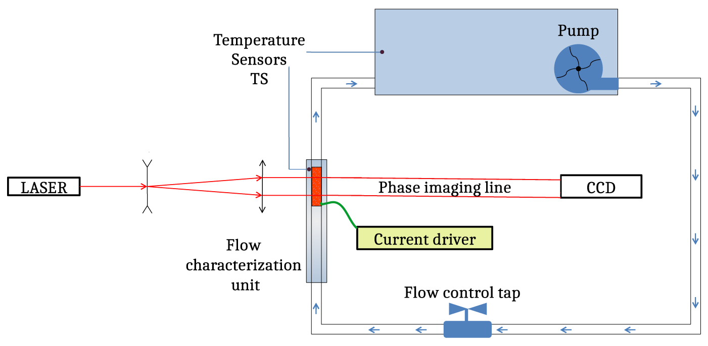
The hydraulic circuit is meant to inject a controllable flow of deionized water into the flow unit by means of a pump delivering a digitally controlled over-pressure and a manual flow control tap. Water exiting the unit enters a large reservoir where it is thermalized to room temperature. The water temperature is monitored by a sensor located within the tank, with a precision of $0.1$
°C. Water is derived from the tap and used after a deionization and filtering step. No pH control appeared to be necessary for these experiments.
$0.1$
°C. Water is derived from the tap and used after a deionization and filtering step. No pH control appeared to be necessary for these experiments.
A rigorous measurement of the volumetric flow rate $F$
is essential for the determination of the fluid velocity within the maquette, and hence of the Reynolds number. Two methods were used: (i) an ultrasonic flow meter for high flows, from
$F$
is essential for the determination of the fluid velocity within the maquette, and hence of the Reynolds number. Two methods were used: (i) an ultrasonic flow meter for high flows, from $2\ \mathrm{L}/\mathrm{min}$
onward, and (ii) chronometry of water filling a calibrated beaker for low flows, namely from zero up to typically
$2\ \mathrm{L}/\mathrm{min}$
onward, and (ii) chronometry of water filling a calibrated beaker for low flows, namely from zero up to typically $4\ \mathrm{L}/\mathrm{min}$
, with a relative accuracy related to the timing precision – hence a somehow cumbersome method, but accurate in absolute value. The intermediate flow region for which both methods are possible was used to calibrate the ultrasonic flow meter, so that absolute flow values could be inferred over the whole range of flows. The average flow velocity within the maquette canal of cross-sectional area
$4\ \mathrm{L}/\mathrm{min}$
, with a relative accuracy related to the timing precision – hence a somehow cumbersome method, but accurate in absolute value. The intermediate flow region for which both methods are possible was used to calibrate the ultrasonic flow meter, so that absolute flow values could be inferred over the whole range of flows. The average flow velocity within the maquette canal of cross-sectional area $S$
is then simply given by
$S$
is then simply given by ${v}_0=F/S$
. The canal transverse sizes were 30 and 40 mm uniformly for maquettes A and B, respectively, so that the hydraulic diameters are almost equal to twice the canal widths.
${v}_0=F/S$
. The canal transverse sizes were 30 and 40 mm uniformly for maquettes A and B, respectively, so that the hydraulic diameters are almost equal to twice the canal widths.
3.2 Amplifier maquettes for flow visualization
Figure 3 presents the two amplifier maquettes used for the hydrodynamic studies of flows in a heated amplifier-like environment. They are designed to image transversely the thermal effects arising along the flows in the laminar and turbulent regimes. Imaging is performed either sideways in the plane of the flow (maquette A) or along the laser axis, orthogonal to the plane of the flow (maquette B). The liquid-cooled laser amplifying medium is replaced by a copper block, or heel, in which two elements are embedded: a heating thermistor (H), in which up to 100 W heat can be generated, and a small (4 mm diameter) temperature sensor (TS). The heel has a flat and highly polished surface, brought into contact with a steady water flow; the temperature sensor is located close to the surface (2 mm) and at the geometrical center of the exchange surface.
Scheme and pictures of the visualization maquettes of forced flows under strong heat load. (a), (b) Maquette A, in-flow transverse imaging setup. (c), (d) Maquette B, laser-axis imaging. Component labels: I, inlet; O, outlet; C, water canal; H, electrical heater; W, optical window; M, copper mirror; L, probe laser; TS, temperature sensor.

Maquette A (cf. Figures 3(a) and 3(b)) thus features a horizontal water canal, 300 mm long, in which the last section before the water outlet corresponds to a 60 mm heated copper surface. The canal width can be varied from 0.5 up to 3 mm; the 240 mm long entrance section is intended to let the turbulence induced by the water injection decay, so that the flow has reached its fully developed profile upon arriving at the heat flux section.
In contrast, the flow plane is vertical in maquette B (cf. Figures 3(c) and 3(d)), with an introduction turbulence decay section of 120 mm that leads the flow onto a 1-inch (1 inch = 2.54 cm) circular mirror, made of copper with a gold layer. This configuration was chosen to allow for optical-quality reflection of the probe laser onto the mirror while keeping an optimal thermal coupling. The probe laser therefore makes a round-trip within the coolant flow, thus doubling the phase disturbances. Indeed, any flow inhomogeneity or turbulence in the incident cold fluid, once in contact with the hot surface, results in the appearance of fluid elements with spatially varying temperatures, leading to inhomogeneous optical indices. We characterize these by a standard strioscopic method, depicted in Figure 4. A helium-neon probe laser, of high spatial quality, goes through the water canals of the various maquettes and then is focused, yielding an intermediate far-field plane in which a mask removes the central spatial frequencies. The standard circular mask of the strioscopic method is replaced here by a needle. Only the higher spatial frequencies, induced by the phase object, in our case the water canal, are transmitted. The exit plane of the water canal is then imaged onto a charge-coupled device (CCD) camera; this yields an image of the phase retardances of the water phase object[ Reference Henares, Puyuelo-Valdes, Hannachi, Ceccotti, Ehret, Gobet, Lancia, Marquès, Santos, Versteegen and Tarisien24, Reference Bruhat and Kastler25].
Principle of the strioscopic technique used to visualize flow index inhomogeneities within the flow characterization unit. Component labels: He:Ne, helium-neon laser; Cu, copper heel; L ${}_1$
and L
${}_1$
and L ${}_2$
, lenses; N, needle; MO, microscope objective; CCD, charge-coupled device camera.
${}_2$
, lenses; N, needle; MO, microscope objective; CCD, charge-coupled device camera.

3.3 In-plane transverse imaging
Maquette A and the strioscopic imaging setup of Figure 4 were used to explore qualitatively how the flow and the boundary layers evolve as the flow speed increases from 0. The onset of the laminar regime, followed by the first signs of flow inhomogeneities, is best seen dynamically on a video, available on Zenodo via Ref. [Reference Féral, Lhermite, Marion, Brandam and Balcou26]. In this video, the coolant is set in motion by gradual opening of the flow control tap from a closed position at time $0$
up to full opening. The indicator on the top left yields the temperature value, in °C, from the temperature sensor.
$0$
up to full opening. The indicator on the top left yields the temperature value, in °C, from the temperature sensor.
From this video, Figures 5 and 6 present snapshots with increasing flow velocities. In Figure 5, the field of view encompasses the entire 3-mm width of the canal; a thermal boundary layer appears clearly on top of the lower wall on all images. The upper wall of the canal should not give rise to strong thermal exchanges; it appears nevertheless on the first images .
Series of transverse strioscopic images of the flow when the water flux is gradually increased from laminar to turbulent, and eventually super-forced thermal regimes. Canal width: 3 mm. Water flows from left to right. Heating occurs on the lower surface. Re = 2100 in (b), Re = 14,000 in (h).

Zoomed image of the heated layer (inverted strioscopic imaging mode) in (a) the laminar regime; (b) instable streaks detached from the wall (Re = 2100); (c) the super-forced thermal regime, with the thermal layer squeezed onto the exchange wall.
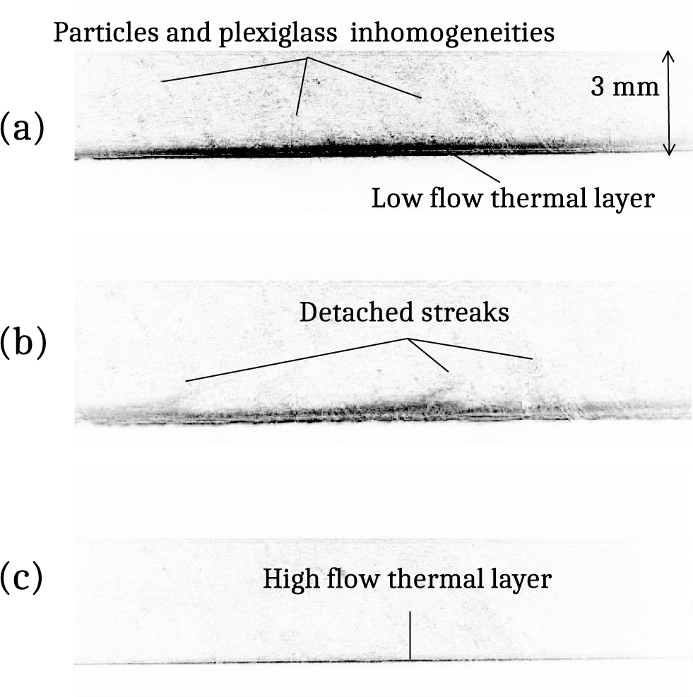
Figure 5(a) corresponds to a slow flow in the laminar regime; one observes clearly an expanding thermal layer with a thickness growing linearly along the flow. In Figure 5(b), ‘plumes’ start to appear above the thermal layer without affecting the previously mentioned linear behavior; irregularities appear in Figure 5(c). The Reynolds number in Figure 5(b) was 2100, as measured in a following experiment stopped at this flow level. Increasing the flow further, the thermal layer becomes turbulent in Figure 5(d), with obvious signs of random eddies in the middle of the flow. Upon increasing the flow further in Figure 5(e), the vortices start earlier and tend to decrease in size. The behavior of the thermal layer is especially striking in Figures 5(f)–5(h), as the eddies appear to be pushed back onto the lower surface and decrease in size and in luminosity. In the final image, Figure 5(h), obtained at the highest flow velocity (Re = 14,000), the thermal layer is squeezed back onto the lower surface, with no irregularity in light diffusion, and is restricted to a thin regular line.
Numerous works in hydrodynamics explain that, once a turbulent regime is set, there is no possibility that the turbulence and the random eddies may vanish upon increasing the flow velocity. What we observe in this optical method are the inhomogeneities of the optical index, resulting from spatial variations in temperature; therefore, we can conclude that, at high velocities, hence well into the weakly turbulent regime, the heat extraction is so efficient that the temperature is actually quasi-homogeneous in the entire canal, except in the immediate vicinity of the heating surface.
The wavefront dephasing on the upper half of the canal, next to the non-heated wall, features an interesting behavior. In Figure 5(a), a second upper thermal layer is clear, which appears along the flow at the same position as the main lower thermal layer; in contrast to the lower layer, its width remains constant and consistent with the upper viscous sub-layer. This linear and thin upper thermal layer is still visible in Figure 5(b), but vanishes at higher flows and is replaced by a broad and homogeneous distribution of thermal dephasings, with its maximum in width and brightness shown in Figures 5(e) and 5(f). The evolution in the upper canal part may be interpreted as resulting from hot fluid elements leaving the main thermal layer where this layer is largest, which then slow down in the upper slow layers of the Poiseuille flow, and possibly setting a thermal equilibrium with the low-effusivity glass that constitutes the upper canal wall. In a real multi-slab amplifier, a similar configuration might arise in the lateral water canals, in between the first and last slabs, and their glass window counterparts.
Figure 6 displays three zoomed images over the thermal layer for increasing flow velocities. For visual clarity, we have inverted the black-and-white color code, thus showing the heated flow regions in black and the cold regions in white. Figure 6(a) corresponds to a laminar regime; the mesh of tiny black spots in the middle of the flow can be assumed to correspond to phase defects in the imaging line itself, possibly in the plexiglass windows, or to defects in the water flow.
Figure 6(b) is taken shortly after the appearance of the first inhomogeneities in the flow; threads of heated water can be seen leaving the thermal layer and are directed to the center of the flow. Finally, Figure 6(c) is a zoomed image of one of the last images of Ref. [Reference Féral, Lhermite, Marion, Brandam and Balcou26], obtained at high flow. This picture shows in a spectacular way how the high flow compresses the thermal layer onto the surface, and displays no sign of the internal flow vortices, known to exist at high velocities. In this super-forced thermal regime, the very high convection effectively bleaches out the effects of thermal inhomogeneities.
3.4 Axial imaging: onset of striation instability
Strioscopic imaging, still transverse to the flow but along the laser axis, allows one to image directly the wavefront perturbations that are imposed on a laser by the flow inhomogeneities. Our results are close to those obtained by Dalbies et al. [ Reference Dalbies, Cavaro, Bouillet, Leymarie, Martin, Cormier, Eupherte, Bordenave, Blanchot, Daurios and Neauport23] with a Foucault-knife approach.
We have used the axial strioscopic setup to shoot movies of the time evolution of the transmitted wavefront. From those movies, we have selected some of the most distinctive images. Figure 7 thus displays the phase perturbations for five different flow velocities, characterized by their Reynolds numbers $\kern0.1em \mathit{\operatorname{Re}}\kern0.1em$
of 1100, 2000, 2300, 5000 and 10,800. The size of the rectangular region of interest displayed is 6.38 mm
$\kern0.1em \mathit{\operatorname{Re}}\kern0.1em$
of 1100, 2000, 2300, 5000 and 10,800. The size of the rectangular region of interest displayed is 6.38 mm $\times$
3.85 mm.
$\times$
3.85 mm.
Near-field views displaying the streamwise streaks for different flow rates and hence different Reynolds numbers: (a) Re = 1100; (b) Re = 2000; (c), (d) Re = 2300; (e) Re = 5000; (f) Re = 10,800. (g) Model stria used to extract the striation level from each image, from a shape recognition method.

The images in Figures 7(b)–7(d) exhibit clear wavefront striae, as reported by Ruan et al. [ Reference Ruan, Su, Tu, Shang, Wu, Yi, Cao, Ma, Wang, Shen, Goa, Zhang and Tang10] and Dalbies et al. [ Reference Dalbies, Cavaro, Bouillet, Leymarie, Martin, Cormier, Eupherte, Bordenave, Blanchot, Daurios and Neauport23]. These striae appear randomly on a black background, meaning that most of the wavefront is undisturbed; striae on these strioscopic phase images indicate that current threads with higher temperature than the surrounding fluid appear in an apparent random way. Such hot current threads can be seen to be essentially parallel to the general direction flow; slight deviation angles with respect to the vertical direction may be seen occasionally, which remain compatible with possible local and transient deviations of the flow.
The images in Figures 7(a), 7(e) and 7(f) show much fainter striae, not necessarily on all images. We have not seen any stria on flows with a Reynolds number of less than 1000. On the high-velocity side, hazy striae can still be perceived at Re = 10,800 on few images. Our setup did not allow us to reach even higher Reynolds numbers.
From each of the numerous images constituting the wavefront movies taken for each Reynolds number, it is necessary to infer a quantitative estimate of the incidence of striae in the region of interest. This required developing a numerical method, mostly based on the well-known OpenCV library of image analysis.
As the striae can be of small amplitude, hardly visible among the noise, it is first necessary to subtract carefully the static background image. The latter is identified by a statistical analysis of the distribution of counts on each pixel of the region of interest after a homothetical reduction by a factor 3. Each background-free image then is subjected to a shape recognition algorithm, in which the template shape is the model stria displayed in Figure 7(g). We use the normalized shape correlation method, which, for each image, outputs a matrix of correlations with the template stria. As the latter is vertical, we take the maximum correlation value for each column; this yields a horizontal correlation function, displayed in blue in Figure 8. Figure 8(f) illustrates the case of a mathematically defined perfect stria, extending vertically at an arbitrary horizontal position. The algorithm correctly presents a correlation peak up to 1 at the central position of the ideal stria, and yields null values on black zones.
Superposition of correlation functions of all images with the model stria for different flow rates: (a) Re = 1100; (b) Re = 2000; (c) Re = 2300; (d) Re = 5000; (e) Re = 10,800. (f) Correlation function between an ideal stria and the stria template.
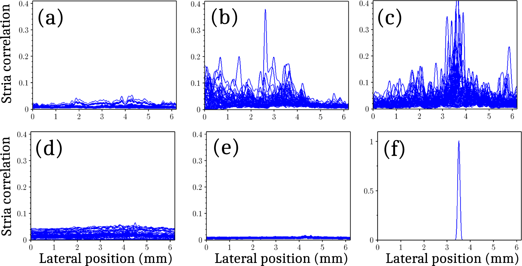
In Figures 8(a)–(e), the striae correlation functions obtained for 100 successive images of the captured movie are superposed for the same Reynolds number as for Figure 7. Each high peak in these correlation functions denotes the existence of one strong stria; different behaviors can be immediately noticed. In Figure 8(c), a strong concentration close to the center of the image is clear; in Figure 8(b), the same zone also features regularly striae, but the left-hand side part of the image also presents many correlation peaks. The distribution of the striae is much more uniform in Figure 8(d). These differing preferential zones of stria appearance may be related to slightly different flow conditions or remaining vorticities for the various velocities. Apart from the preferential zones, one also notices that there is no fixed or repeated position; hence, the striae are not formed on a specific defect sites upstream, but rather appear randomly. We should mention however that, in early designs, we did observe occasionally striae arising at a fixed position, suggesting they can also stem from surface defects; only after a careful mechanical design to remove any such defect did we observe the randomness in striae positions.
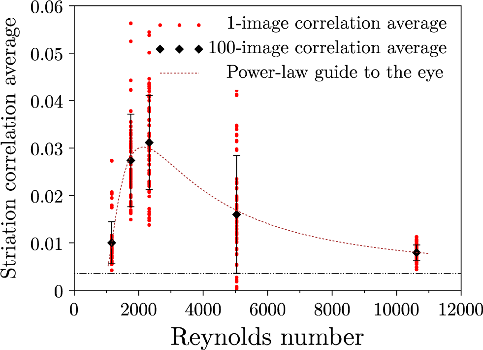
Figure 9 displays the average values of the striae correlation function for each of the 100 images (red points) and the overall average of the average values (black diamond) as a function of the Reynolds numbers of the five flows studied. The background images yield a low but non-zero average of the spatial correlation function; hence, the bottom line indicated using dashes. No striae are seen below $\kern0.1em \mathit{\operatorname{Re}}=1000$
; then, the average striae correlation grows suddenly up to a maximum around 2500. The measured striae then start decreasing down to almost zero for
$\kern0.1em \mathit{\operatorname{Re}}=1000$
; then, the average striae correlation grows suddenly up to a maximum around 2500. The measured striae then start decreasing down to almost zero for $\kern0.1em \mathit{\operatorname{Re}}\simeq 10,000$
. The dotted line is a simple guide to the eye, taken as the product of two power law dependencies, one increasing sharply from
$\kern0.1em \mathit{\operatorname{Re}}\simeq 10,000$
. The dotted line is a simple guide to the eye, taken as the product of two power law dependencies, one increasing sharply from $\kern0.1em \mathit{\operatorname{Re}}=1000$
on, and one decreasing steadily from zero.
$\kern0.1em \mathit{\operatorname{Re}}=1000$
on, and one decreasing steadily from zero.
Reynolds number dependence of the average striae correlation. Dashed bottom line: residual correlation with the random background of the images, which defines the lower limit of significant correlations.
3.5 Discussion of the optical striation instability and hydrodynamic streaks
The appearance of striae in face cooling was not anticipated, and their physical origin remains uncertain. Some authors mention them as an effect of turbulence; we suggest that these striae are the result of a hydrodynamic instability, in the same range of Reynolds numbers as the TSI, but they are well distinct from weak turbulence. Indeed, in an axial view, the striae appear as extremely straight and regular over lengths possibly exceeding several centimeters – as demonstrated by Dalbies et al. [ Reference Dalbies, Cavaro, Bouillet, Leymarie, Martin, Cormier, Eupherte, Bordenave, Blanchot, Daurios and Neauport23]. No meandering was observed, although the striae may appear as not fully parallel to the main flow in rare cases. This seems, however, incompatible with the random interplay of flow vortices inherent to a turbulent regime.
Secondly, the striae do not systematically appear; some pictures were essentially free of any striation, while other pictures show striae in some areas and no wavefront perturbations in others. Again, this is not the behavior of a turbulent flow.
Thirdly, we observe a sudden rise in the prevalence of striations from $\kern0.1em \mathit{\operatorname{Re}}=1000$
onward, whereas the results of the following section on heat exchanges demonstrate the onset of the weakly turbulent regime at
$\kern0.1em \mathit{\operatorname{Re}}=1000$
onward, whereas the results of the following section on heat exchanges demonstrate the onset of the weakly turbulent regime at $\kern0.1em \mathit{\operatorname{Re}}\simeq 2700$
, consistent with the standard values reported in the scientific literature[
Reference Gnielinski11,
Reference Versteeg and Malalasekera12,
Reference Bergman, Lavine, Incropera and Dewitt20].
$\kern0.1em \mathit{\operatorname{Re}}\simeq 2700$
, consistent with the standard values reported in the scientific literature[
Reference Gnielinski11,
Reference Versteeg and Malalasekera12,
Reference Bergman, Lavine, Incropera and Dewitt20].
We conclude that the striae are the result of a pre-transitional hydrodynamic instability, and not of weak turbulence. This leaves open the issue of the physical origin of this instability.
We propose at this stage a naming convention: in the optical community, the long lines observed are most often called ‘striae’, consistent with the fact that they are actually phase retardances observed by strioscopy or any equivalent technique. In the hydrodynamics community, long linear structures are usually called streaks, and are thought of as a line of current with different velocities, pressures and shear concentrations to the surrounding flow. We suggest keeping both words, using ‘striae’ whenever we refer to the optical structures and ‘streaks’ when we refer to the underlying hydrodynamical structure.
To the best of our knowledge, the streaks within the boundary layer of a Poiseuille flow at an early stage of the laminar-to-turbulent transition did not attract much interest in the field of hydrodynamics and of heat exchanges. The situation is, however, different for Blasius flows, with a number of works studying the physics of longitudinal flow streaks and their role in the chain of processes that eventually trigger turbulence (see Ref. [Reference Boiko, Grek, Dovgal and Kozlov18] by Boiko et al., Chapter 9, and references therein).
As concerns specifically Poiseuille flows, as an introduction to his work on the induction of instabilities in the plane Poiseuille flow, Mizushima[ Reference Mizushima27] does not mention any case of streak formation; in contrast, his first-principle calculations result in the well-known TSI, that is, rows of vortices of alternate helicities with axes transverse to the flow, as illustrated by Figure 9 of Barahona et al. [ Reference Barahona, Rius-Vidales, Tocci, Ziegler, Hein and Kotsonis28]. Many other contributions explore the physics of the TSI. From this body of work, we can conclude that TSI waves and face-cooling striae display entirely different geometries, and are therefore two distinct processes.
From the scientific literature on hydrodynamics of unstable plane flows, we found however two processes displaying current streaks in Poiseuille flows.
Several studies have indeed been devoted to the ‘low-speed streaks’ appearing in transitional planar flows at higher Reynolds numbers; these streaks were first observed by Kline et al. [ Reference Kline, Reynolds, Schraubt and Runstadler29], and were subject later to extensive research works reviewed by Lee and Wu[ Reference Lee and Wu30]. In addition to the higher Reynolds regime, the characteristics of those low-speed streaks are wholly different: they present a high level of self-organization with an initial regular pattern, similar intensities and quickly display meandering and mixing behaviors. None of these features are observed on the striae seen in face cooling.
In the laminar regime of natural convection between a heated vertical wall and a passive wall, Čolak-Antić and Görtler[ Reference Čolak-Antić and Görtler31] reported on vertical striae with a visual appearance extremely similar to that of face cooling. The striae were first observed in a low Reynolds laminar regime (Figure 3(a) of Ref. [Reference Čolak-Antić and Görtler31]), then in conjunction with TSI waves at larger Reynolds numbers – confirming these are two different processes, starting at different Reynolds numbers in natural convection.
The existence and role of streamwise streaks in Blasius flows, of direct interest in aerodynamics, has received much more attention[
Reference Boiko and Chun32]. In his textbook, Boiko surveys several instabilities observed in pre-transitional flows in addition to TSI waves: $\Lambda$
-shaped structures, turbulent spots and puffs resulting from a well-studied lift-up mechanism, and may extend over many characteristic lengths
$\Lambda$
-shaped structures, turbulent spots and puffs resulting from a well-studied lift-up mechanism, and may extend over many characteristic lengths $d$
in the streamwise direction. This feature makes puffs interesting candidates to explain the striae observed in liquid face cooling, provided the physics in Blasius flows can be extended to Poiseuille flows. However, the striae could also result from a process that couples thermal and hydrodynamic processes through the temperature dependence of density and viscosity.
$d$
in the streamwise direction. This feature makes puffs interesting candidates to explain the striae observed in liquid face cooling, provided the physics in Blasius flows can be extended to Poiseuille flows. However, the striae could also result from a process that couples thermal and hydrodynamic processes through the temperature dependence of density and viscosity.
More detailed hydrodynamical studies would hence be required to ascertain the intrinsic nature of the striation instability. In the scope of the present study, we merely point out that some instabilities, such as the puff instability, coupled to a hot wall, might result in the appearance of streaks with a differential heating from the main flow resulting in locally different temperatures, inducing wavefront distortions by virtue of the temperature dependence of the refractive index.
4 Experimental study of the heat exchange coefficient in laser amplifier-relevant conditions
We now turn to the study of the heat exchange coefficients, or Nusselt numbers, based on a third maquette design, allowing one to control the amount of heat deposited in the coolant and to measure precisely the inner temperature, and input and output water temperatures.
4.1 Measurement method for the heat exchange coefficient
Maquette C, schematized in Figure 10(a) and pictured in Figure 10(b), is designed to perform the measurement of the exchange coefficient in flow and thermal load conditions similar to those of a multi-slab laser amplifier.
Scheme (a) and pictures (b) of the exchange coefficient measurement maquette. Component labels: I, inlet; O, outlet; H, electrical heater; TS, temperature sensor.

The thermal heel is a $20$
-mm-thick copper block, whose exchange surface with the liquid coolant is a rectangle of
$20$
-mm-thick copper block, whose exchange surface with the liquid coolant is a rectangle of $24$
mm (along the flow) by
$24$
mm (along the flow) by $50$
mm (transverse to the flow). As the overall and measured exchange coefficient depends on the length of the exchange zone along the flow, this rectangular geometry allows us to infer an unambiguous
$50$
mm (transverse to the flow). As the overall and measured exchange coefficient depends on the length of the exchange zone along the flow, this rectangular geometry allows us to infer an unambiguous $h$
coefficient.
$h$
coefficient.
Figure 11(a) shows a semi-transparent view of the copper block (yellow), positioned in an optically transparent but thermally isolating poly(methyl methacrylate) (PMMA) optical window (grey). The exchange surface (ES) is grazing the inner surface of the optical window in order to prevent any induced vorticity in the water flow. The temperature sensor (TS) is embedded deeply within the copper block, just $2$
mm from the exchange surface. In a coordinate frame where
$2$
mm from the exchange surface. In a coordinate frame where $x$
and
$x$
and $y$
are respectively transverse and along the flow, with an origin at the center of the exchange rectangle, the temperature sensor stands at
$y$
are respectively transverse and along the flow, with an origin at the center of the exchange rectangle, the temperature sensor stands at $x=0$
and
$x=0$
and $y=+5$
mm. The heater is a cylinder-shaped resistor, also embedded within the copper block. These mechanical details happen to have an importance to compute the apparatus response function.
$y=+5$
mm. The heater is a cylinder-shaped resistor, also embedded within the copper block. These mechanical details happen to have an importance to compute the apparatus response function.
Numerical calibration of the exchange coefficient $h$
. (a) Geometry of the 3D numerical twin. H, heater; TS, temperature sensor; ES, exchange surface. (b) Normalized temperature profiles predicted for different target values of
$h$
. (a) Geometry of the 3D numerical twin. H, heater; TS, temperature sensor; ES, exchange surface. (b) Normalized temperature profiles predicted for different target values of $h$
; inset, temperature profile over the exchange surface, from cyan (coldest) to red (hottest) for
$h$
; inset, temperature profile over the exchange surface, from cyan (coldest) to red (hottest) for $h$
= 10,000
$h$
= 10,000 $\mathrm{W}\ {\mathrm{m}}^{-2}\ {\mathrm{K}}^{-1}$
. (c) Exchange coefficient predicted to be measured versus input exchange coefficient.
$\mathrm{W}\ {\mathrm{m}}^{-2}\ {\mathrm{K}}^{-1}$
. (c) Exchange coefficient predicted to be measured versus input exchange coefficient.

Indeed, the heat exchange coefficient $h$
is defined as follows[
Reference Bergman, Lavine, Incropera and Dewitt20]:
$h$
is defined as follows[
Reference Bergman, Lavine, Incropera and Dewitt20]:
 $$\begin{align}h=\frac{P_\mathrm{th}}{S\left({T}_\mathrm{av}-{T}_0\right)},\end{align}$$
where ${P}_\mathrm{th}$
is the thermal power load,
${P}_\mathrm{th}$
is the thermal power load, $S$
is the exchange surface and
$S$
is the exchange surface and ${T}_\mathrm{av}$
is the average temperature on the exchange surface; meanwhile, the experiment yields an exchange coefficient as follows:
${T}_\mathrm{av}$
is the average temperature on the exchange surface; meanwhile, the experiment yields an exchange coefficient as follows:
 $$\begin{align*}{h}_{\mathrm{measured}}=\frac{P_\mathrm{th}}{S\left({T}_\mathrm{TS}-{T}_0\right)},\end{align*}$$
where ${T}_\mathrm{TS}$
is the temperature as measured by the embedded temperature sensor, which is not strictly equal to the average temperature on the exchange surface. This systematic error is expected to be small, since we chose copper as constituent material, the high thermal conductivity of which should lead to an optimally homogeneous temperature over the block. However, the heat flow is never homogeneous – neither for our device, which includes a localized heater and an insertion hole for the temperature sensor; nor for a real laser amplifier slab, for which the heat flow depends on the volumetric heat generation. Moreover, the heat flux can also be partly evacuated by channels other than conduction through the exchange surface with the coolant. Such corrections are again expected to be minor, but should be evaluated. All these processes are related to thermal conduction and exchanges in the copper block, which are well known, and can be modeled numerically with high accuracy.
${T}_\mathrm{TS}$
is the temperature as measured by the embedded temperature sensor, which is not strictly equal to the average temperature on the exchange surface. This systematic error is expected to be small, since we chose copper as constituent material, the high thermal conductivity of which should lead to an optimally homogeneous temperature over the block. However, the heat flow is never homogeneous – neither for our device, which includes a localized heater and an insertion hole for the temperature sensor; nor for a real laser amplifier slab, for which the heat flow depends on the volumetric heat generation. Moreover, the heat flux can also be partly evacuated by channels other than conduction through the exchange surface with the coolant. Such corrections are again expected to be minor, but should be evaluated. All these processes are related to thermal conduction and exchanges in the copper block, which are well known, and can be modeled numerically with high accuracy.
To determine the response function, we therefore use a numerical twin of the setup, by means of a COMSOL simulation. Starting from a given exchange coefficient $h$
, and for an arbitrary heater power, we compute the temperature profile in the block, then the temperature
$h$
, and for an arbitrary heater power, we compute the temperature profile in the block, then the temperature ${T}_\mathrm{TS}$
at the position of the sensor, leading to a numerical evaluation of
${T}_\mathrm{TS}$
at the position of the sensor, leading to a numerical evaluation of ${h}_{\mathrm{measured}}$
.
${h}_{\mathrm{measured}}$
.
Figure 11(b) shows the normalized temperature profile $\left(T-{T}_0\right)/\left({T}_{\mathrm{max}}-{T}_0\right)$
on a line of the exchange surface in the
$\left(T-{T}_0\right)/\left({T}_{\mathrm{max}}-{T}_0\right)$
on a line of the exchange surface in the $y$
direction parallel to the flow and going through the sensor (
$y$
direction parallel to the flow and going through the sensor ( $x=0$
), for different exchange coefficients, from a low value (
$x=0$
), for different exchange coefficients, from a low value ( $500$
W m−2 K−1) up to a high value (
$500$
W m−2 K−1) up to a high value ( $10,000$
W m−2 K−1). We took a constant copper-to-air exchange coefficient of 50 W m−2 K−1. At low exchange coefficients, the profile can be seen to be regular and close to
$10,000$
W m−2 K−1). We took a constant copper-to-air exchange coefficient of 50 W m−2 K−1. At low exchange coefficients, the profile can be seen to be regular and close to $1$
, implying that the sensor provides a satisfactory estimate for the mean temperature; in contrast, high exchange coefficients lead to somewhat lower temperatures and more pronounced inhomogeneities. The inset shows a false-color map of the temperature over the exchange surface, from cyan to red, for the highest exchange coefficient. A temperature minimum, and a kink in the profile, appear right below the position of the temperature sensor, leading to a noticeable deviation between the temperature at the sensor position and the average temperature.
$1$
, implying that the sensor provides a satisfactory estimate for the mean temperature; in contrast, high exchange coefficients lead to somewhat lower temperatures and more pronounced inhomogeneities. The inset shows a false-color map of the temperature over the exchange surface, from cyan to red, for the highest exchange coefficient. A temperature minimum, and a kink in the profile, appear right below the position of the temperature sensor, leading to a noticeable deviation between the temperature at the sensor position and the average temperature.
Figure 11(c) displays the numerical prediction of the measured exchange coefficient as a function of the exchange coefficient taken as input. To help the eye, the dot-dashed line shows for comparison the identity curve: ${h}_{\mathrm{measured}}=h$
. The response function appears fairly linear, with however a small quadratic term that leads to a deviation of up to 10% for the highest values of
${h}_{\mathrm{measured}}=h$
. The response function appears fairly linear, with however a small quadratic term that leads to a deviation of up to 10% for the highest values of $h$
. A small constant term results from the cooling action of air convection at the copper-to-air interfaces, which is negligible for high values of
$h$
. A small constant term results from the cooling action of air convection at the copper-to-air interfaces, which is negligible for high values of $h$
.
$h$
.
This response function can now be inverted to correct the experimental exchange coefficients presented in the next section.
4.2 Experimental results of heat exchange coefficients
Figure 12 shows the experimental data of heat exchange coefficients obtained with maquette C, with a water canal of 0.54 mm width (Figure 12(a)) and 1.1 mm width (Figure 12(b)). In the latter case, two independent measurement series were performed several days apart, and are labeled measurement set 1 (circles) and set 2 (dots).
Experimental data for the exchange coefficient (a) for a 0.54 mm water canal and (b) for a 1.1 mm water canal. Fits with power law functions are displayed with red dashes. In Section 5.3, the experimental data are compared with the combination of the best estimates from computational fluid dynamics, as given by Equation (7), displayed as a continuous dark blue line.

We supply error bars along both the abscissa and ordinate. The uncertainties of the flow velocities result (i) from the uncertainty of the flow measurement with the chronometry method, estimated to $\pm 5\%$
(timing uncertainty about 1 s over 20 s, meniscus height of the water surface of 1 mm in a 150-mm beaker); and (ii) from the uncertainty of the width of the canal, estimated to
$\pm 5\%$
(timing uncertainty about 1 s over 20 s, meniscus height of the water surface of 1 mm in a 150-mm beaker); and (ii) from the uncertainty of the width of the canal, estimated to $\pm 25\;\unicode{x3bc} \mathrm{m}$
in absolute value. Combining these uncertainties results in velocity error bars of
$\pm 25\;\unicode{x3bc} \mathrm{m}$
in absolute value. Combining these uncertainties results in velocity error bars of $\pm 7\%$
and
$\pm 7\%$
and $\pm 6\%$
for the 0.54 and 1.1 mm canals, respectively. The uncertainties of
$\pm 6\%$
for the 0.54 and 1.1 mm canals, respectively. The uncertainties of $h$
are related to the 0.1 K resolution of the temperature sensors, to the existence of thermal leaks in the hydraulic system and to the numerical uncertainty of the response function explained in Section 4.1. In practice, we observe a typical scatter of data points up to 5
$h$
are related to the 0.1 K resolution of the temperature sensors, to the existence of thermal leaks in the hydraulic system and to the numerical uncertainty of the response function explained in Section 4.1. In practice, we observe a typical scatter of data points up to 5 $\%$
, and a similar gap shows up between data sets 1 and 2 of the 1.1 mm canal, taken independently. We choose therefore error bars of
$\%$
, and a similar gap shows up between data sets 1 and 2 of the 1.1 mm canal, taken independently. We choose therefore error bars of $\pm 10\%$
in the
$\pm 10\%$
in the $h$
data.
$h$
data.
The empirical correlations of $h$
given in the literature are always based on a power law on the Reynolds number; the power law exponent is an important element that distinguishes between flow regimes. We present therefore power law fits on the data. In Figure 12(a), the fit, shown with red dash-dots, matches very well with the data over the whole measurement range, with Reynolds numbers ranging from 0 to 2400. The power law exponent thus determined is 0.40.
$h$
given in the literature are always based on a power law on the Reynolds number; the power law exponent is an important element that distinguishes between flow regimes. We present therefore power law fits on the data. In Figure 12(a), the fit, shown with red dash-dots, matches very well with the data over the whole measurement range, with Reynolds numbers ranging from 0 to 2400. The power law exponent thus determined is 0.40.
In Figure 12(b), the data present an obvious kink at a flow velocity around 1.1 m/s. We therefore performed a fit for lower velocity values (red dash-dots), yielding a power law exponent of 0.35; and another one for higher velocities (purple long dashes), yielding a power law exponent of 0.81.
We interpret the kink in Figure 12(b) as the obvious manifestation of the flow regime transition from laminar to weakly turbulent.
5 Comparison with numerical estimates of the exchange coefficient
The experimental data are to be compared with computational results from common numerical methods of computational fluid dynamics (CFD) on the basis of standard models that can be exploited by all laser scientists without recourse to excessively complex algorithmic tools or requiring overwhelming computation times. This requires, however, bringing together thermal transfer within the coolant, NS equations describing fluid motion and possibly direct absorption within the coolant of the pump light, laser light and amplified spontaneous emission. Full coolant modeling should hence be ideally coupled to modeling of the laser materials, optical windows and mounts – an ensemble well beyond the scope of the present study[ Reference Yi, Tu, An, Ruan, Wu, Su, Shang, Yu, Liao, Cao, Cui, Gao and Zhang7, Reference Yang13, Reference Lin, Zhu, Zhao, Qiao, Wang, Wang and Zhu33].
In the framework of the LEAP-Horizon project[ Reference Lhermite, Féral, Marion, Rohm, Balcou, Descamps, Petit, Nadeau and Mével34], we chose to resort to the COMSOL Multiphysics version 5.4 software suite, allowing easy coupling to subsequent material analysis and optical calculations. Only the thermal exchange description, which is part of the COMSOL kernel, and the CFD module are used in the following.
We restricted ourselves to model the coolant flows with a few well-known approaches: direct numerical solution (DNS) of the NS equations, usually only possible in the laminar regime; the ${y}^{+}$
mixing length model; the Reynolds-Average Navier–Stokes (RANS)
${y}^{+}$
mixing length model; the Reynolds-Average Navier–Stokes (RANS) $k-\epsilon$
model[
Reference Versteeg and Malalasekera12]; the shear stress transport (SST) model; and a stationary LES approach. Note that we assume throughout the flow to be stationary.
$k-\epsilon$
model[
Reference Versteeg and Malalasekera12]; the shear stress transport (SST) model; and a stationary LES approach. Note that we assume throughout the flow to be stationary.
5.1 Overview of computational fluid dynamic algorithms used
All CFD models for an incompressible fluid start from the mass continuity and from the NS equation, written as follows:
 $$\begin{align}\nabla .\left(\rho \mathbf{u}\right)&=0,\end{align}$$
 $$\begin{align}\rho \left(\mathbf{u}.\nabla \right)\mathbf{u}&=-\nabla P+\nabla \mu \left(\nabla \mathbf{u}+{\left(\nabla \mathbf{u}\right)}^\mathrm{T}\right)-\frac{2}{3}\nabla \left(\mu \left(\nabla .\mathbf{u}\right)\right),\end{align}$$
where $\mathbf{u}$
is the flow velocity field,
$\mathbf{u}$
is the flow velocity field, $P$
is the pressure field,
$P$
is the pressure field, $\mu$
is the dynamic viscosity and
$\mu$
is the dynamic viscosity and $\rho$
is the fluid density function. We choose to neglect in Equation (5) any effect of buoyancy – the role of buoyancy in the fluid dynamics of an amplifier head is complex[
Reference Chen and Chung35], and would deserve further studies, especially for slow flows.
$\rho$
is the fluid density function. We choose to neglect in Equation (5) any effect of buoyancy – the role of buoyancy in the fluid dynamics of an amplifier head is complex[
Reference Chen and Chung35], and would deserve further studies, especially for slow flows.
Equation (4) results from mass conservation in an incompressible fluid, while Equation (5) expresses conservation of momentum in a Newtonian fluid with dynamical viscosity $\mu$
, yielding a viscosity shear stress tensor
$\mu$
, yielding a viscosity shear stress tensor $K$
, as the last term of Equation (5).
$K$
, as the last term of Equation (5).
These fluid equations must be completed by the water heat capacity equation and by the stationary heat conduction and convection equation:
 $$\begin{align}\rho {C}_\mathrm{p}\mathbf{u}.\nabla T-\nabla \cdot\left(\lambda \nabla T\right)=0,\end{align}$$
where $\lambda$
and
$\lambda$
and ${C}_\mathrm{p}$
are the thermal conductivity and specific heat capacity at constant pressure of water, respectively, and the temperature and velocities should be taken as the average values in the case of a RANS-type model such as
${C}_\mathrm{p}$
are the thermal conductivity and specific heat capacity at constant pressure of water, respectively, and the temperature and velocities should be taken as the average values in the case of a RANS-type model such as $k-\epsilon$
.
$k-\epsilon$
.
From this core set of equations, the following standard CFD approaches were investigated.
-
• These equations are directly solved with the direct numerical simulation approach. This is known to yield accurate solutions in the laminar regime, corresponding in most cases to Reynolds numbers lower than 2300. Laminarity does not mean unidirectional motion, however, as the results may indicate a flow regime with recirculation areas, for instance next to the edges of a laser crystal disk or in any dead end or corner of the water circulation zone. As the Reynolds number increases, the software spends an increased amount of time to converge to a steady-state solution; ultimately, the calculation no longer converges, which appears as the numerical signature of the onset of weak turbulence. One has to stop the calculation after a fixed number of iterations, which in practice still yields nice-looking results, the significance of which is however limited in the turbulent regime.
-
• The mixing length model, or $y^{+}$
model, is the most simple and numerically efficient approach. This model assumes that the velocity fluctuations beyond the viscous sub-layer undergo a simple diffusion-like process over a mixing length
$l$
equivalent to a ‘mean free path’. The model assumes that
$l$
is null in the viscous sub-layer and increases beyond it linearly as
$l=\kappa y$
, where
$\kappa \simeq 2.5$
is the von Karman constant and
$y$
is the distance to the nearest wall[
Reference Guyon, Hulin, Petit and Mitescu16]. The Reynolds stresses can then be estimated analytically on the basis of the solution of coupled algebraic laws on a normalized velocity
${u}^{+}=u/{u}_{\ast }$
, where
$u$
is the flow velocity, and on a normalized spatial dimension
${y}^{+}=y/{y}_{\ast }$
. Here,
${u}_{\ast }$
is the friction velocity,
${u}_{\ast}=\sqrt{\left( \mathrm{d}u/ \mathrm{d}y\right)\mu /\rho }$
, and
${y}_{\ast }$
is essentially the local width of the viscous sub-layer. In the model case of a Blasius flow, namely, a flow with uniform velocity impinging on a single plate parallel to the flow, this model predicts a logarithmic behavior of the flow velocity beyond the viscous sub-layer up to the domain where the velocity saturates to the incoming flow velocity.
$y^{+}$
model, is the most simple and numerically efficient approach. This model assumes that the velocity fluctuations beyond the viscous sub-layer undergo a simple diffusion-like process over a mixing length
$l$
equivalent to a ‘mean free path’. The model assumes that
$l$
is null in the viscous sub-layer and increases beyond it linearly as
$l=\kappa y$
, where
$\kappa \simeq 2.5$
is the von Karman constant and
$y$
is the distance to the nearest wall[
Reference Guyon, Hulin, Petit and Mitescu16]. The Reynolds stresses can then be estimated analytically on the basis of the solution of coupled algebraic laws on a normalized velocity
${u}^{+}=u/{u}_{\ast }$
, where
$u$
is the flow velocity, and on a normalized spatial dimension
${y}^{+}=y/{y}_{\ast }$
. Here,
${u}_{\ast }$
is the friction velocity,
${u}_{\ast}=\sqrt{\left( \mathrm{d}u/ \mathrm{d}y\right)\mu /\rho }$
, and
${y}_{\ast }$
is essentially the local width of the viscous sub-layer. In the model case of a Blasius flow, namely, a flow with uniform velocity impinging on a single plate parallel to the flow, this model predicts a logarithmic behavior of the flow velocity beyond the viscous sub-layer up to the domain where the velocity saturates to the incoming flow velocity. -
• The RANS approach is intended to predict turbulence levels without capturing their temporal evolution, but estimates the mean turbulence content of the flow. We report calculations with the most standard
$k-\epsilon$
approach, but we also tested the closely related
$k-\omega$
approach and the shear stress transport model, often considered to blend the advantages of
$k-\epsilon$
and
$k-\omega$
.In the RANS approach, the velocity field
$\mathbf{u}$
, the pressure field
$P$
and the temperature field
$T$
are assumed to be the sum of a slowly varying term and of a fast randomly varying term, whose time-average is zero. Still assuming the fluid to be incompressible, this results in a modified NS equation that requires the introduction of two new physical quantities: the turbulent kinetic energy
$k$
and the turbulence energy decay rate
$\epsilon$
. The viscosity stress tensor
$K$
is then modified to include a turbulent viscosity term, added to the standard kinematic viscosity. The set of equations is closed by two convection equations for
$k$
and
$\epsilon$
, with ad hoc parameters[
Reference Versteeg and Malalasekera12]; a turbulent convection term is also added to the heat conduction–convection in Equation (6).


-
• LESs are usually time-dependent simulations, akin to DNS simulations, thus allowing one to describe the spatial and temporal evolution of turbulent vortices, also called eddies. The largest eddies are entirely simulated; however, the energy transfer cascade of large eddies to smaller and smaller eddies is interrupted by a numerical filter, and ad hoc estimates are used to evaluate the residual Reynolds stresses. We made use of the LES approach with the residual-based variational multiscale with viscosity (RBVMWV) method to evaluate the effect of the smaller vortices. The multiphysics software uses a pseudo-time approach to converge to a stationary solution. While LES calculations are known to require high CPU times, our experience does not show an excessive computing load, but an issue of lack of convergence, similar to the DNS approach.
Following Ref. [Reference Nagymihály, Cao, Papp, Hajas, Kalashnikov, Osvay and Chvykov15], we point out that the use of so-called ‘wall functions’[ Reference Schlichting and Gersten19], possibly installed by default in the CFD software, should be avoided to compute any heat exchange coefficient. Indeed, in many engineering applications, the flow behavior immediately next to the wall has little importance, and the wall functions allow one to skip the detailed calculations in the viscous sub-layer at the expense of the appearance of discontinuities in dynamic and thermodynamic variables at the wall. Figure 15, in Section 5.2, will show that use of a wall function results in a velocity field that does not respect the no-slip condition. The resulting predictions for thermal exchange rates do not make sense.
Finally, we recall that CFD methods have a number of intrinsic limitations, as underlined by Refs. [Reference Versteeg and Malalasekera12,Reference Tu, Yeoh and Liu17]. Most CFD models rely on specific approximations to describe turbulence, the validity of which may be difficult to evaluate. The DNS approach stands out as it does not involve any model of turbulence; however, its successful implementation might be difficult[ Reference Versteeg and Malalasekera12]. Secondly, CFD models may be oversimplified with respect to the experimental reality and neglect such factors as surface roughness, interfacial layers, incident vorticity, etc. Thirdly, multiphysics tools employing CFD, such as COMSOL, have reached a very high degree of sophistication that actually decreases the scientist’s ability to check the subtle numerical interconnections between intertwined physical processes.
5.2 Numerical implementation
The CFD approaches described above are applied to a test geometry, depicted in Figure 13, which reproduces the most important features of the experiment while keeping a moderate computing time.
Two-dimensional modeling geometry and set of initial conditions: input velocity (left blue arrow), heat flux (green), initial water temperature (black); output numerical diagnostics: average metal surface temperature and mass-averaged output fluid temperature.

Our 2D model features a water canal with two parts: a long entrance duct, aimed to let the decay of any vortex induced by the injection conditions and mimic the experimentally imposed flux calming section; and a part in which the fluid is in contact with a heated metallic heel in its upper part.
The canal width and interface length reproduce the experimental values ( $0.54$
or
$0.54$
or $1.1$
mm). The entrance canal length can be taken as identical to the interface length, or longer. In all cases, the flow at the entrance of the exchange region was checked to have reached a stationary average velocity profile.
$1.1$
mm). The entrance canal length can be taken as identical to the interface length, or longer. In all cases, the flow at the entrance of the exchange region was checked to have reached a stationary average velocity profile.
All boundaries, except the heat injection surface, the exchange interface and the fluid input and output, are thermally isolated (thick lines). The heat flux $\mathrm{d}Q/ \mathrm{d}S$
is injected uniformly on the upper heel surface
$\mathrm{d}Q/ \mathrm{d}S$
is injected uniformly on the upper heel surface $S$
, goes through the metallic layer, of conductivity
$S$
, goes through the metallic layer, of conductivity ${\lambda}_\mathrm{c}$
and width
${\lambda}_\mathrm{c}$
and width ${d}_\mathrm{c}$
, and then through the thermal layer of the flow. In a 2D geometry, the heat injection surface or exchange surface is given by the common heel and interface length
${d}_\mathrm{c}$
, and then through the thermal layer of the flow. In a 2D geometry, the heat injection surface or exchange surface is given by the common heel and interface length $L$
, taken to correspond to the experimental value (
$L$
, taken to correspond to the experimental value ( $L=24$
mm). The heel thickness is taken as
$L=24$
mm). The heel thickness is taken as $5$
mm, smaller than the experimental one – it was checked that this parameter did not play any significant role. Calling
$5$
mm, smaller than the experimental one – it was checked that this parameter did not play any significant role. Calling ${T}_\mathrm{S}$
the average temperature at the water–metal interface and
${T}_\mathrm{S}$
the average temperature at the water–metal interface and ${T}_0$
the initial water temperature, the numerical exchange coefficient is calculated as
${T}_0$
the initial water temperature, the numerical exchange coefficient is calculated as $h={P}_\mathrm{th}/S\left({T}_\mathrm{S}-{T}_0\right)$
.
$h={P}_\mathrm{th}/S\left({T}_\mathrm{S}-{T}_0\right)$
.
Numerical convergence was checked on all parameters with respect to the height of the heel, to the incident velocity profile of the incoming flow and to the value of the injected power. Of particular importance was the definition of the numerical mesh in the thermal layer, namely, the first few hundred micrometers immediately below the exchange surface. Figure 14 displays the typical mesh used for the converged computations; while the general mesh follows a triangle structure, we resorted to a very fine rectangular mesh in the thermal layer with cell heights starting at $3$
$3$ $\unicode{x3bc}$
m and increasing exponentially up to
$\unicode{x3bc}$
m and increasing exponentially up to $70$
$70$ $\unicode{x3bc}$
m, corresponding to the general triangular mesh of the water flow. These figures are both commensurate with the distance
$\unicode{x3bc}$
m, corresponding to the general triangular mesh of the water flow. These figures are both commensurate with the distance ${y}_{\mathit{\operatorname{Re}}=1}$
to the wall that results in a local Reynolds number
${y}_{\mathit{\operatorname{Re}}=1}$
to the wall that results in a local Reynolds number $v(y)y/\nu$
of 1:
$v(y)y/\nu$
of 1: ${y}_{\mathit{\operatorname{Re}}=1}\simeq 10$ $\unicode{x3bc}$
m, which is an estimate of the local Kolmogorov length scale. Similarly, a fine mesh (
$\unicode{x3bc}$
m, which is an estimate of the local Kolmogorov length scale. Similarly, a fine mesh ( $\simeq 70$ $\unicode{x3bc}$
m) over the remaining water flow turned out to be necessary to reach converged exchange coefficients. In contrast, a rough mesh within the heel was sufficient, with the COMSOL meshing algorithm forcing the mesh size close to the interface to match that of the flow. Numerical convergence with respect to mesh parameters was checked independently in each mesh region: the triangular mesh general flow region, rectangular mesh thermal layer, triangular mesh metallic heel.
$\unicode{x3bc}$
m) over the remaining water flow turned out to be necessary to reach converged exchange coefficients. In contrast, a rough mesh within the heel was sufficient, with the COMSOL meshing algorithm forcing the mesh size close to the interface to match that of the flow. Numerical convergence with respect to mesh parameters was checked independently in each mesh region: the triangular mesh general flow region, rectangular mesh thermal layer, triangular mesh metallic heel.
Numerical mesh: zoomed onto the entrance region to the thermal interface layer. The metallic heel sits at the top; the lower region is the water canal.

Figure 15 shows the transverse velocity distributions of a fully established Poiseuille flow, from analytical theory (green); direct numerical simulations (black dots); the mixing length ${y}^{+}$
model (red); RANS with (blue, dot-dashed) and without (blue, continuous) wall functions; and LES simulation (magenta, dot-dashed). Even in the laminar regime, the velocity profile appears flattened by all CFD computations with respect to the theoretical Poiseuille profile. The agreement between
${y}^{+}$
model (red); RANS with (blue, dot-dashed) and without (blue, continuous) wall functions; and LES simulation (magenta, dot-dashed). Even in the laminar regime, the velocity profile appears flattened by all CFD computations with respect to the theoretical Poiseuille profile. The agreement between ${y}^{+}$
and DNS is excellent; the RANS
${y}^{+}$
and DNS is excellent; the RANS $k-\epsilon$
results with wall functions are completely different from all others.
$k-\epsilon$
results with wall functions are completely different from all others.
Transverse velocity profiles at Re = 2000, as computed by the various CFD models examined: theoretical Poiseuille profile, DNS, mixing length model, RANS $k-\epsilon$
with and without wall function and large-eddy simulation with the residual-based variational multiscale with viscosity method.
$k-\epsilon$
with and without wall function and large-eddy simulation with the residual-based variational multiscale with viscosity method.

5.3 Comparisons between experimental data, model-dependent numerical estimates, and empirical correlations
The numerical results from the DNS (red line), ${y}^{+}$
, RANS
${y}^{+}$
, RANS $k-\epsilon$
, SST and LES calculations can now be compared with our experimental data. The latter are reproduced in Figure 16 as black dots, without the error bars, for canals of 0.54 mm (cf. Figure 16(a)) and 1.1 mm (cf. Figure 16(b)).
$k-\epsilon$
, SST and LES calculations can now be compared with our experimental data. The latter are reproduced in Figure 16 as black dots, without the error bars, for canals of 0.54 mm (cf. Figure 16(a)) and 1.1 mm (cf. Figure 16(b)).
Comparisons between experimental data (same data as in Figure 12) for the exchange coefficient (a) for a 0.54 mm water canal and (b) for a 1.1 mm water canal, and numerical models or empirical laws.

The DNS and ${y}^{+}$
turn out to be exactly superposed. Their results display the same ‘square-root’ aspect as the experimental data for the 0.54 mm canal, and for the 1.1 mm data up to a velocity of around 1.1 m/s. Agreement is excellent with the latter data; the DNS or
${y}^{+}$
turn out to be exactly superposed. Their results display the same ‘square-root’ aspect as the experimental data for the 0.54 mm canal, and for the 1.1 mm data up to a velocity of around 1.1 m/s. Agreement is excellent with the latter data; the DNS or ${y}^{+}$
curve stands above the 0.54 mm data, with a 15% relative difference in the Re = 1000 range, which remains close to the estimated error bars. While no definitive explanation of the deviation between the DNS and the 0.54 mm experimental data points can be found, we suspect that a thin oxide layer may have developed over the exchange surface in the course of the 0.54 mm canal experiment, leading to a slightly reduced exchange coefficient.
${y}^{+}$
curve stands above the 0.54 mm data, with a 15% relative difference in the Re = 1000 range, which remains close to the estimated error bars. While no definitive explanation of the deviation between the DNS and the 0.54 mm experimental data points can be found, we suspect that a thin oxide layer may have developed over the exchange surface in the course of the 0.54 mm canal experiment, leading to a slightly reduced exchange coefficient.
The SST and LES RMVMWV calculations happen to yield similar values of $h$
, which are consistent with, and slightly larger than, the DNS or
$h$
, which are consistent with, and slightly larger than, the DNS or ${y}^{+}$
results. No kink is observed on any of these four models.
${y}^{+}$
results. No kink is observed on any of these four models.
In contrast, the RANS $k-\epsilon$
model predictions do not match the data for the 0.54 mm canal; for the 1.1 mm one, they correctly fit the data for velocities higher than 1.2 m/s, or Reynolds numbers larger than 2700. Our RANS
$k-\epsilon$
model predictions do not match the data for the 0.54 mm canal; for the 1.1 mm one, they correctly fit the data for velocities higher than 1.2 m/s, or Reynolds numbers larger than 2700. Our RANS $k-\omega$
predictions are almost identical to the RANS
$k-\omega$
predictions are almost identical to the RANS $k-\epsilon$
ones; the
$k-\epsilon$
ones; the $k-\omega$
model does not present any specific advantage with respect to the
$k-\omega$
model does not present any specific advantage with respect to the $k-\epsilon$
one to describe laser face cooling.
$k-\epsilon$
one to describe laser face cooling.
Interestingly, in Figure 16(b), the ${y}^{+}$
and RANS
${y}^{+}$
and RANS $k-\epsilon$
models intersect at the position of the kink in the experimental data. For the 0.54 mm canal, the intersection between
$k-\epsilon$
models intersect at the position of the kink in the experimental data. For the 0.54 mm canal, the intersection between ${y}^{+}$
and RANS results occurs at a Reynolds number around 2200, close to the highest Reynolds values of the experimental data.
${y}^{+}$
and RANS results occurs at a Reynolds number around 2200, close to the highest Reynolds values of the experimental data.
From this comparison, we conclude that the 0.54 mm canal data were taken entirely in a laminar regime; the flow conditions for the 1.1 mm canal are first laminar, then switch to weakly turbulent, and from that point on, are correctly described by the RANS $k-\epsilon$
model.
$k-\epsilon$
model.
This can be understood as follows. In the laminar regime, the exact DNS method fully converges and is the most relevant to describe the heat exchange; once the weakly turbulent regime sets in, the DNS fails to converge rigorously and is no longer able to describe adequately the effect of vortices in the flow. In contrast, RANS models such as $k-\epsilon$
and
$k-\epsilon$
and $k-\omega$
compute the time-averaged effect of eddies and the associated turbulent transport, even when there are actually no eddies around in the laminar regime. The prediction of the RANS
$k-\omega$
compute the time-averaged effect of eddies and the associated turbulent transport, even when there are actually no eddies around in the laminar regime. The prediction of the RANS $k-\epsilon$
model is therefore meaningless in the laminar regime, but becomes meaningful in the weakly turbulent regime, leading to a sudden change in the functional dependence of the exchange coefficient with respect to the Reynolds number. Such a sudden switch was reported by Gnielinski[
Reference Gnielinski11] at the laminar to turbulent transition at Re = 2300.
$k-\epsilon$
model is therefore meaningless in the laminar regime, but becomes meaningful in the weakly turbulent regime, leading to a sudden change in the functional dependence of the exchange coefficient with respect to the Reynolds number. Such a sudden switch was reported by Gnielinski[
Reference Gnielinski11] at the laminar to turbulent transition at Re = 2300.
This reasoning and the known change of behavior at the laminar to turbulent transition lead us to suggest a simple means to compute the exchange coefficient by 2D CFD:
 $$\begin{align}h=\sup \left({h}_{y^{+}},{h}_{\mathrm{RANS}\;k-\epsilon} \right),\end{align}$$
where we use the ${y}^{+}$
approach in the laminar range instead of DNS, since
${y}^{+}$
approach in the laminar range instead of DNS, since ${y}^{+}$
has no convergence issues and yields the same results for
${y}^{+}$
has no convergence issues and yields the same results for $h$
as the DNS.
$h$
as the DNS.
Figure 12 allows us to compare Equation (7) with the experimental data and the fits. For the shallowest canal, the CFD prediction is slightly higher than the data, by about 20%; the kink does not appear experimentally, but the expected transition is within the velocity error bars of the last data point. For the 1.1 mm canal, these combined CFD predictions fit remarkably the data.
This simple equation, which remains to be evaluated in other flow conditions, might be in practice the most useful take-away message of our heat exchange studies.
The analytical laws or empirical correlations do not match as well the experimental data, but are however interesting and potentially useful to yield estimates without recourse to CFD numerical tools. We therefore test against our data two analytical laws supposed to fit the heat exchange in the laminar regime and two in the turbulent regime.
In his textbook, Koechner[ Reference Koechner36] advises to consider the correlation supplied by Mann and Weber in 1988[ Reference Mann and Weber37], who used the formula proposed by Chen et al. in 1946[ Reference Chen, Hawkins and Solberg38]. The equation was derived from experimental data for heat transfer in annuli; going to the limit where the annulus radii of curvature reach infinity yields the following relation:
 $$\begin{align}{h}_{\mathrm{Chen}}={C}_\mathrm{L}\frac{k}{d_\mathrm{h}}{\left(\frac{d}{L}\right)}^{0.4}\kern0.1em {\mathit{\Pr}}^{0.33}\kern0.1em {\mathit{\operatorname{Re}}}^{0.45}\kern0.1em \mathrm{Gr}^{0.05},\end{align}$$
where $L$
is the length of the heat exchange section;
$L$
is the length of the heat exchange section; $\kern0.1em \mathrm{Gr}\kern0.1em$
is the Grashof number, characteristic of buoyancy effects and free convection; and
$\kern0.1em \mathrm{Gr}\kern0.1em$
is the Grashof number, characteristic of buoyancy effects and free convection; and ${C}_\mathrm{L}$
is a numeric factor. While Mann and Weber advise to take
${C}_\mathrm{L}$
is a numeric factor. While Mann and Weber advise to take ${C}_\mathrm{L}=0.5\pm 0.1$
, we used in Figure 16 a value of
${C}_\mathrm{L}=0.5\pm 0.1$
, we used in Figure 16 a value of ${C}_\mathrm{L}=1.02$
, as in the original publication by Chen et al. The dependence on the Grashof number, although weak, creates two issues, conceptual and practical: (i) why does this correlation include a term of natural convection, while the experiments are made in a forced convection regime; and (ii) the Grashof number depends on the temperature difference between the wall and liquid, which is an a priori unknown value: given a heat deposition rate in a laser amplifier, the temperature difference results from the heat exchange coefficient, which is the value we wish to evaluate. To bypass this loop, our estimate in Figure 16 makes use of the temperature difference obtained numerically by the
${C}_\mathrm{L}=1.02$
, as in the original publication by Chen et al. The dependence on the Grashof number, although weak, creates two issues, conceptual and practical: (i) why does this correlation include a term of natural convection, while the experiments are made in a forced convection regime; and (ii) the Grashof number depends on the temperature difference between the wall and liquid, which is an a priori unknown value: given a heat deposition rate in a laser amplifier, the temperature difference results from the heat exchange coefficient, which is the value we wish to evaluate. To bypass this loop, our estimate in Figure 16 makes use of the temperature difference obtained numerically by the ${y}^{+}$
approach with a heat load matching that of our experiment. This somehow cumbersome procedure actually supplies qualitatively reasonable estimates (purple thin dotted line), above the experimental data for the 0.54 mm canal and below them for the 1.1 mm canal.
${y}^{+}$
approach with a heat load matching that of our experiment. This somehow cumbersome procedure actually supplies qualitatively reasonable estimates (purple thin dotted line), above the experimental data for the 0.54 mm canal and below them for the 1.1 mm canal.
We also compare the results with the Colburn correlation in laminar regime, as advised by the textbook by Battaglia et al. [ Reference Battaglia, Kosika and Puiggali22]:
 $$\begin{align}{h}_{\mathrm{Colburn}}^{\mathrm{lam}}=1.86\frac{k}{d_\mathrm{h}}{\left(\frac{\kern0.1em \mathit{\operatorname{Re}}\cdot \mathit{\Pr}\cdot {d}_\mathrm{h}}{L}\right)}^{0.33}{\left(\frac{\mu }{\mu_\mathrm{s}}\right)}^{0.14},\end{align}$$
where $\mu$
is the fluid dynamical viscosity at its average temperature in the canal and
$\mu$
is the fluid dynamical viscosity at its average temperature in the canal and ${\mu}_\mathrm{s}$
is the fluid dynamic viscosity at the wall temperature. Following Mann and Weber[
Reference Mann and Weber37], we simply assume
${\mu}_\mathrm{s}$
is the fluid dynamic viscosity at the wall temperature. Following Mann and Weber[
Reference Mann and Weber37], we simply assume $\mu ={\mu}_\mathrm{s}$
, which amounts to a small temperature difference approximation. The resulting numerical estimate of the laminar Colburn is represented by orange thin dashes; it overestimates the heat exchange for the 0.54 mm canal and underestimates it for the 1.1 mm canal, like the Chen correlation (cf. Equation (8)), but to a significantly lesser extent. The functional dependence on the velocity, that is, the power law behavior, is also better than that observed with the Chen correlation.
$\mu ={\mu}_\mathrm{s}$
, which amounts to a small temperature difference approximation. The resulting numerical estimate of the laminar Colburn is represented by orange thin dashes; it overestimates the heat exchange for the 0.54 mm canal and underestimates it for the 1.1 mm canal, like the Chen correlation (cf. Equation (8)), but to a significantly lesser extent. The functional dependence on the velocity, that is, the power law behavior, is also better than that observed with the Chen correlation.
In the weakly turbulent regime, we propose comparisons with the empirical correlation by Gnielinsky[ Reference Gnielinski39], as was suggested by Yang[ Reference Yang13], and with the Colburn turbulent correlation[ Reference Battaglia, Kosika and Puiggali22]:
 $$\begin{align}{h}_{\mathrm{Colburn}}^{\mathrm{turb}}=0.023\frac{k}{d_\mathrm{h}}\kern0.1em {\mathit{\operatorname{Re}}}^{0.8}\kern0.22em {\mathit{\Pr}}^{0.33}.\end{align}$$
The power law in the Reynolds number is quite close to that obtained in our power law fit of the data. This function is represented by thin brown dashes; for the 0.54 mm canal, it does not fit the data, which makes sense since the flow regime was laminar and the function is supposed to be valid in a weak turbulence regime. For the 1.1 mm canal, it does run parallel to those experimental data points after the kink in the curve. It overestimates slightly the $h$
coefficient; however, its main drawback is that the intersection with the Colburn laminar correlation does not seem to match the position of the kink observed experimentally.
$h$
coefficient; however, its main drawback is that the intersection with the Colburn laminar correlation does not seem to match the position of the kink observed experimentally.
The Gnielinski correlation reads as follows[ Reference Yang13, Reference Gnielinski39]:
 $$\begin{align}{h}_{\mathrm{Gni}}=\frac{k_\mathrm{f}\cdot F}{d_\mathrm{h}}\left(\kern0.1em \mathit{\operatorname{Re}}-1000\right)\frac{\kern0.1em \mathit{\Pr}\kern0.1em }{1+12.7\sqrt{F}\left(\kern0.1em {\mathit{\Pr}}^{2/3}-1\right)},\end{align}$$
where $F={\left(1.82\times {\log}_{10}\kern0.1em \mathit{\operatorname{Re}}-1.64\right)}^{-2}/8$
. This function is represented by thin dark green dashes. In contrast to the Colburn turbulent correlation, this estimate does not start at the origin, but rather at
$F={\left(1.82\times {\log}_{10}\kern0.1em \mathit{\operatorname{Re}}-1.64\right)}^{-2}/8$
. This function is represented by thin dark green dashes. In contrast to the Colburn turbulent correlation, this estimate does not start at the origin, but rather at $\kern0.1em \mathit{\operatorname{Re}}=1000$
. The intersection with the laminar curve for the 1.1 mm canal occurs around
$\kern0.1em \mathit{\operatorname{Re}}=1000$
. The intersection with the laminar curve for the 1.1 mm canal occurs around $\kern0.1em \mathit{\operatorname{Re}}=3000$
, consistent with the experimental kink position.
$\kern0.1em \mathit{\operatorname{Re}}=3000$
, consistent with the experimental kink position.
The overall agreement between these correlations and the experimental data is less satisfactory than between CFD calculations and the data. From this set of comparisons, we can suggest that the following relation, mimicking Equation (7), might still be of practical interest to design face-cooling systems without recourse to CFD tools:
 $$\begin{align}h=\sup \left({h}_{\mathrm{Colburn}}^{\mathrm{lam}},{h}_{\mathrm{Gni}}\right).\end{align}$$
6 Conclusions
From these studies, amplifier maquettes were quite useful to gain insight into the physics of face cooling of laser multi-slab amplifiers.
-
• From benchmarking the results of CFD computations and analytical or empirical correlations with the experimental data for heat exchanges, we conclude that the mixing length
${y}^{+}$
model is effective to predict exchange rates in the laminar regime; and that the RANS
$k-\epsilon$
model is effective to predict exchange rates in the weakly turbulent range. As soon as turbulence sets in, the Nusselt number is dominated by the turbulent eddies. Our proposed formula in Equation (7) should therefore supply good estimates over all regimes. Equations (9), (11) and (12) can be used together as a fast estimator, but CFD computations turned out to be much more reliable than analytical correlations. -
• In the conditions of face cooling of amplifiers, the pre-transitional range of Reynolds numbers plays a crucial role. All laboratories testing face cooling have observed striae. From our axial and side phase images, we point out that these are not an effect of turbulence, but rather are a pre-transitional hydrodynamic instability, which, in our experimental conditions and following the usual engineering definition of the Reynolds number, starts at
$\kern0.1em \mathit{\operatorname{Re}}=1000$
, whereas the heat exchange measures clearly see the onset of turbulence around
$\kern0.1em \mathit{\operatorname{Re}}=2700$
. Figure 9 actually shows that the striae start to decrease at that Reynolds number, indicating that the onset of turbulence may correspond to a break-up of the streaks. Our side-imaging movie shows that, in our specific conditions of water face cooling, turbulence may be triggered by the detachment from the wall and consequent break-up of the streaks, and not by the usual TS route.The striae, or underlying current streaks, appear randomly, with however preferential zones of prevalence, which vary with the average flow velocity, possibly pointing out a relation with residual velocity-dependent vorticity of the incident flow. The hydrodynamic nature of these pre-transitional streaks remains to be understood.


-
• Our experiments have revealed the interest of the Reynolds number range beyond 10,000. In this super-forced thermal regime, the thermally affected zone within the flow remains restricted to a thin layer on the exchange surface and the striation effect tends to vanish.
To design a water face-cooled laser amplifier, the laser scientist must suppress, or at least strongly mitigate, the striation effect. From our studies, three strategies can be envisioned.
-
• Bleach optically the striae, by resorting to the index-leveling method proposed by Marion et al. [ Reference Marion, Balcou, Féral, Rohm and Lhermite40].
-
• A shallow canal approach: remain at Reynolds numbers less than 1000 by decreasing the distance between the slabs or that between the slab and window. Reaching values less than 0.5 mm may, however, be difficult from a mechanical design perspective, which should effectively limit the heat exchange coefficients to ca. 6000 W m−2 K−1.
-
• Increase strongly the hydraulic pump pressure to accelerate dramatically the flow and reach the super-forced thermal regime. The latter should, however, be the subject of further studies, which entails several experimental challenges. Hydraulic systems should be developed, able to inject flows with hydraulic pressures of few bars into millimetric or sub-millimetric single or multiple canals while keeping precise pressure equilibria to prevent mechanical damage. Other challenges involve the fast time scales required to diagnose the index inhomogeneities and the reduced index differences.
The first strategy can actually be combined with either of the other two; therefore, we are confident that these conclusions can pave the way to new generations of high-energy laser amplifiers with average powers in the multi-kW range or higher. Many further studies would still be highly beneficial on the physics of the striation instability, on the super-forced thermal regime and on the extremely complex effects of buoyancy in laser face-cooling systems.
Acknowledgements
This work is part of the LEAP project, supported by Région Nouvelle-Aquitaine (contracts 16005645 and 8384920), and by the European Structural and Investment Funds (contracts 2779610 and 7609710).
It was also supported by CNRS Innovation under the Turbocool project (2022–2023).
Funding and human resources dedicated to the LEAP project, as well as administration by Université de Bordeaux, CEA, CNRS and CELIA administrative unit are gratefully acknowledged. The authors also wish to acknowledge the mechanical expertise of Laurent Merzeau and Franck Blais and to thank them for the precise fabrication of the various maquettes used in this work; and the contribution to experiments and simulations of J. Brandam, A. Mêlé, M. Taleb-Ali and J. Patfoort.

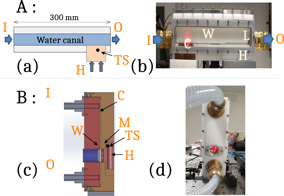
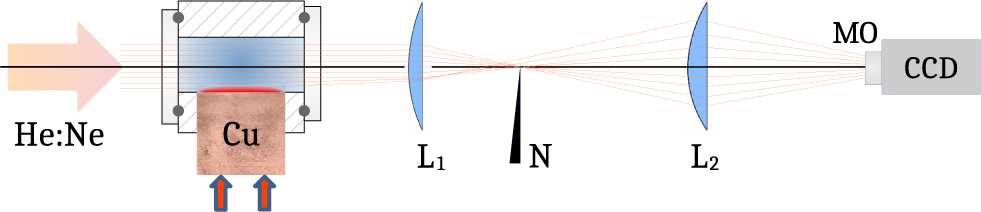


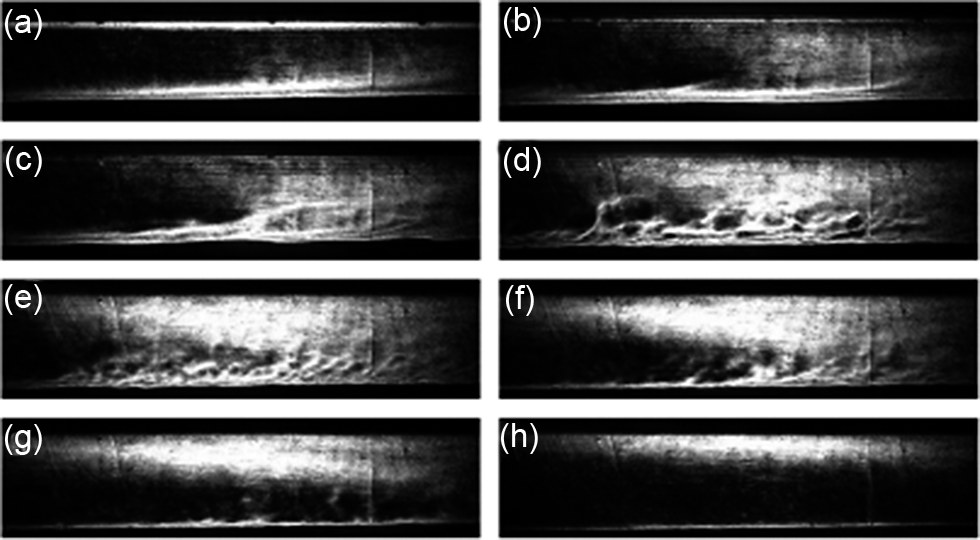

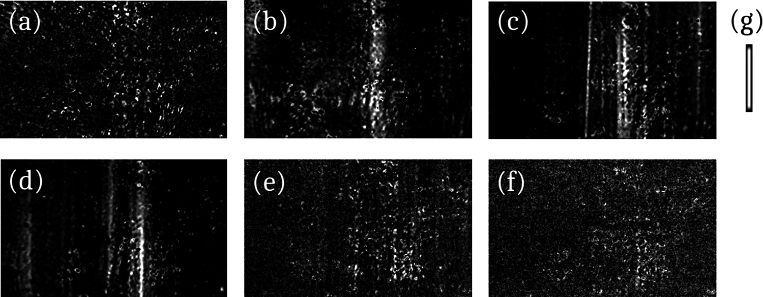


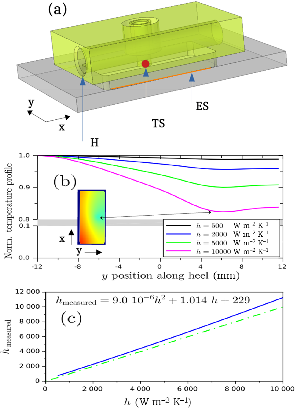


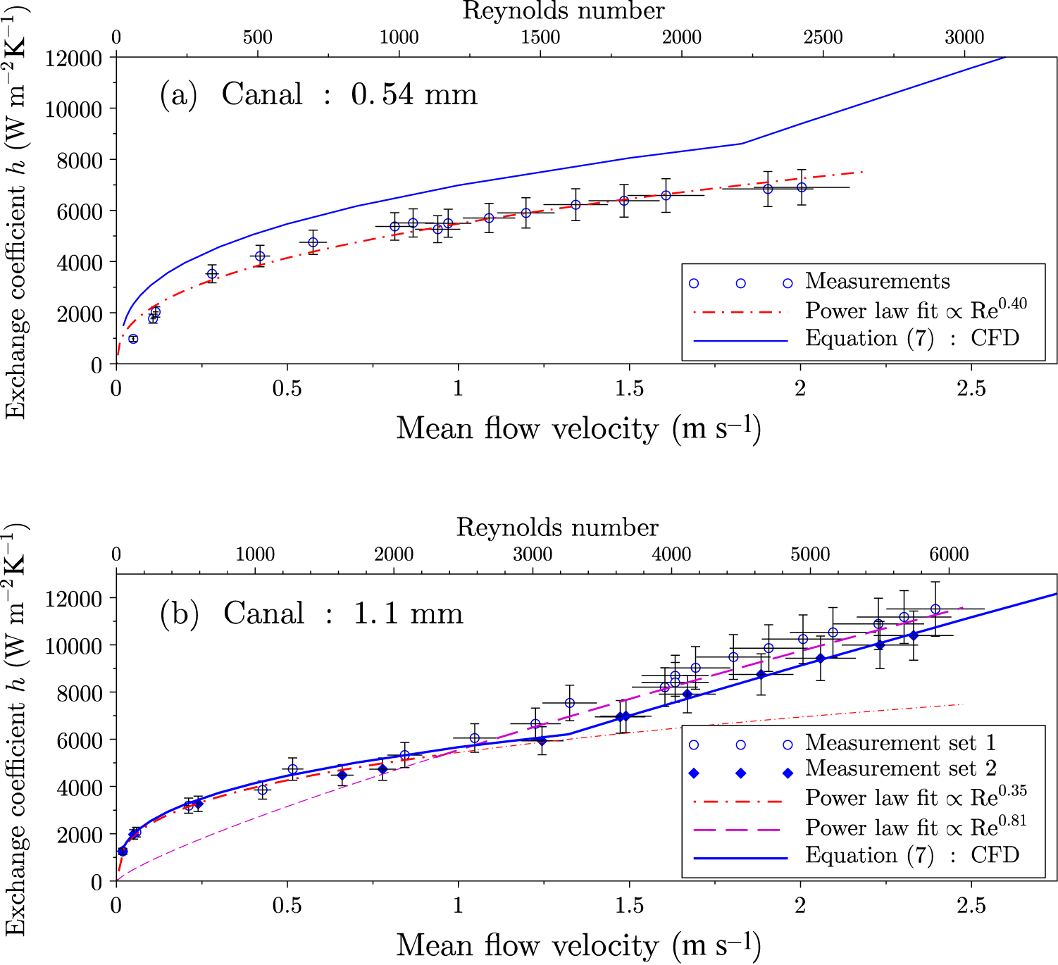
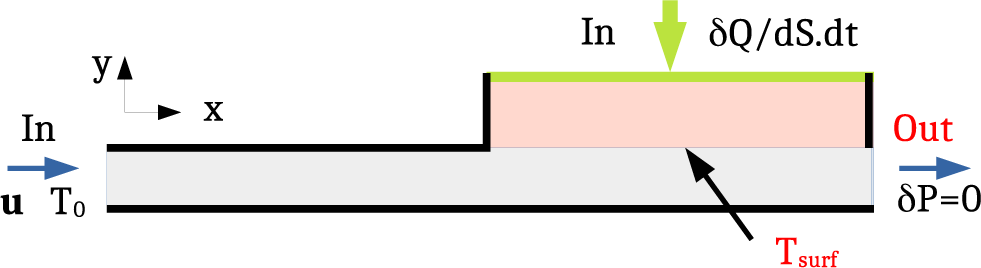
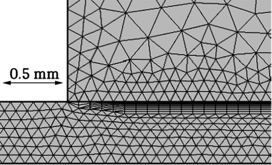
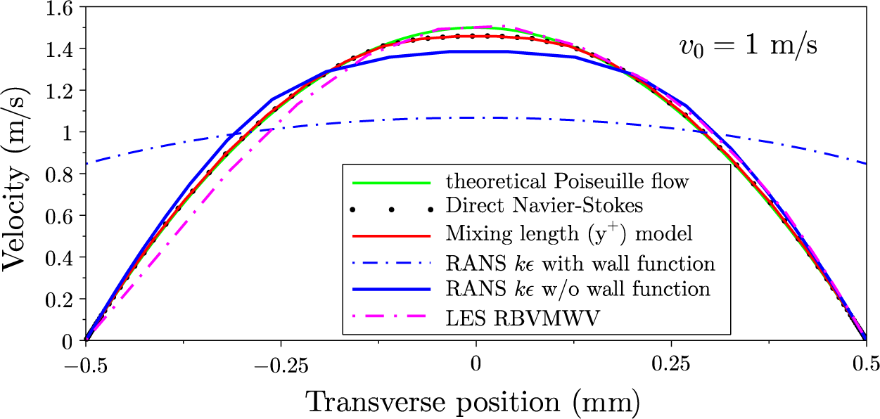

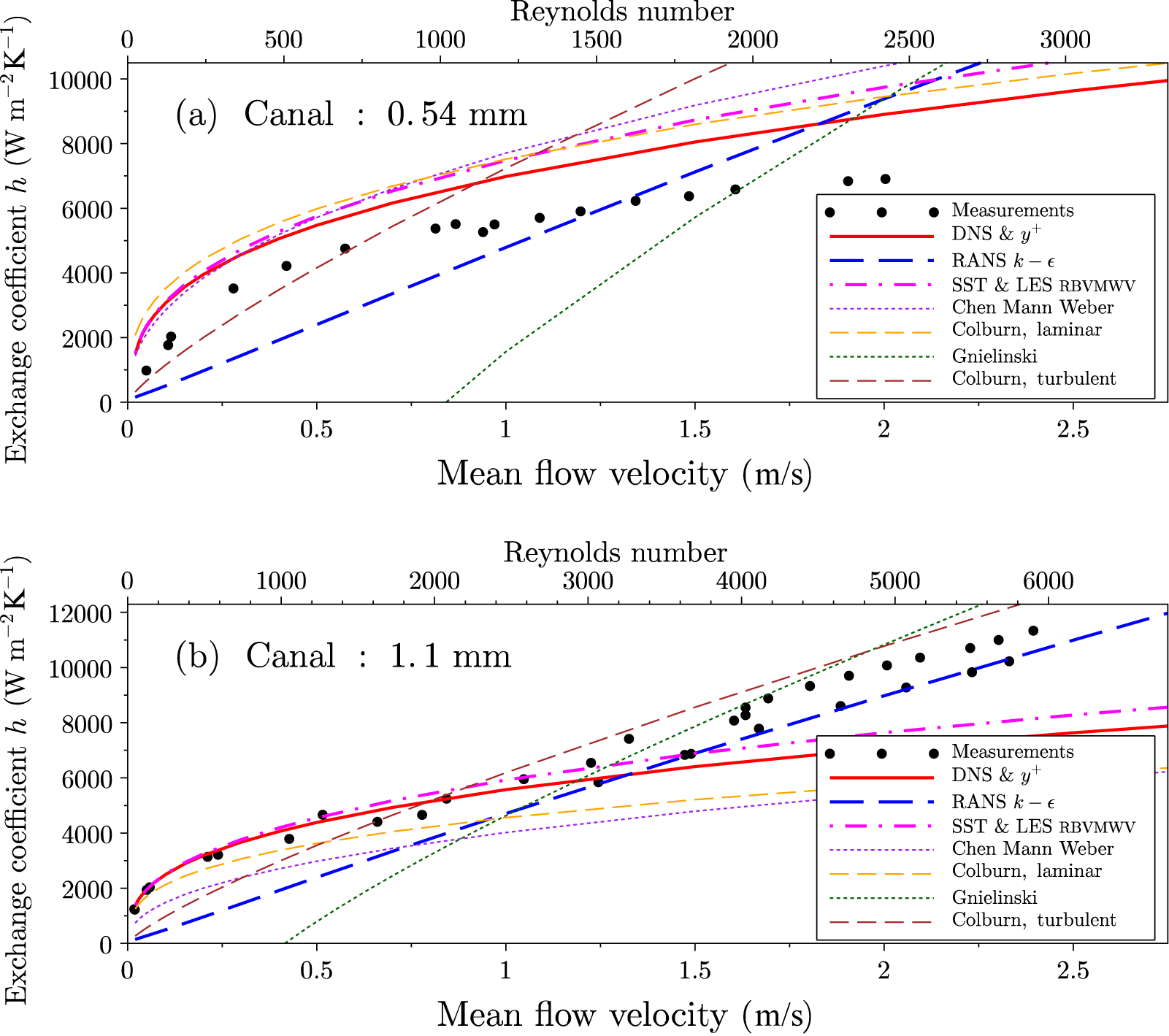

 Open access