


1. Introduction
Two-fluid plane Couette flows were first shown by Yih (Reference Yih1967) to be unstable to long waves at non-zero Reynolds numbers. The instability depends on the viscosity and thickness ratios of the two layers. Subsequent analyses established the ‘thin-layer effect’ – namely that if the thin layer is more viscous, the flow is linearly unstable (Hooper & Boyd Reference Hooper and Boyd1983; Hooper & Grimshaw Reference Hooper and Grimshaw1985; Renardy Reference Renardy1985, Reference Renardy1987). Weakly nonlinear reductions connected these results to dispersive Kuramoto–Sivashinsky-type amplitude equations (Hooper & Grimshaw Reference Hooper and Grimshaw1985, Reference Hooper and Grimshaw1988; Charru & Fabre Reference Charru and Fabre1994). We are motivated by certain key experimental observations of Barthelet, Charru & Fabre (Reference Barthelet, Charru and Fabre1995), who studied wave formation in a two-fluid annular Couette device driven by a rotating upper lid. The depth of the device’s annulus is smaller than its width, and so a two-dimensional assumption is reasonable, at least away from end walls. The geometry of the experiment is ideal for comparisons to certain nonlinear reduced dimension evolution equation models for several reasons: (i) observed waves are periodic with a period at most equal to the perimeter, $L_w$
say, of the annulus; (ii)
$L_w$
say, of the annulus; (ii) $L_w$
unambiguously sets the period to be used in model equations; and (iii) any bifurcations from unimodal, i.e.
$L_w$
unambiguously sets the period to be used in model equations; and (iii) any bifurcations from unimodal, i.e. $L_w$
-periodic, to bimodal
$L_w$
-periodic, to bimodal $({1}/{2})L_w$
-periodic waves arise naturally and are within reach of analytical descriptions. Indeed, Barthelet et al. (Reference Barthelet, Charru and Fabre1995) reported long-wave asymmetry and, at higher upper-lid speeds, the existence of bistability, with unimodal and bimodal travelling waves coexisting.
$({1}/{2})L_w$
-periodic waves arise naturally and are within reach of analytical descriptions. Indeed, Barthelet et al. (Reference Barthelet, Charru and Fabre1995) reported long-wave asymmetry and, at higher upper-lid speeds, the existence of bistability, with unimodal and bimodal travelling waves coexisting.
Recent modelling developments have introduced an inertia-retaining non-local model for two-layer Couette flow, in which the thick lower layer enters via an Orr–Sommerfeld problem at leading order (Kalogirou et al. Reference Kalogirou, Cîmpeanu, Keaveny and Papageorgiou2016; Kalogirou & Papageorgiou Reference Kalogirou and Papageorgiou2016), enabling quantitative comparisons at experimentally relevant Reynolds numbers.
We also note closely related mathematical studies that use the same travelling wave machinery in analogous settings: Papageorgiou & Tanveer (Reference Papageorgiou and Tanveer2019) developed and analysed a non-local model when the thin layer is the lower one; Katsiavria & Papageorgiou (Reference Katsiavria and Papageorgiou2022) incorporated interfacial slip in multilayer shear flows and examined its impact on nonlinear wave selection; and Papageorgiou & Tanveer (Reference Papageorgiou and Tanveer2023) demonstrated that even modest interfacial slip can have a singular effect in otherwise stable two-layer shear flows. This finding was shown to be quite generic in the linear stability study of the full problem by Katsiavria & Papageorgiou (Reference Katsiavria and Papageorgiou2024). In the presence of pressure-driven flow, analogous techniques can be used to derive and study model equations and compare results with simulations – see Kalogirou, Cîmpeanu & Blyth (Reference Kalogirou, Cîmpeanu and Blyth2020), Kalogirou & Blyth (Reference Kalogirou and Blyth2023).
The models used in this study are asymptotically valid for a thin, more viscous upper layer lying over a thick, denser layer, e.g. mineral oil/glycerine–water systems used in the experiments. Hence, this study focuses on reproducing reported experiments with thickness ratio $d=0.25$
, where
$d=0.25$
, where $d$
is the ratio of the mean upper layer thickness to that of the lower one. The value
$d$
is the ratio of the mean upper layer thickness to that of the lower one. The value $d=0.25$
is the smallest one reported in the experiments and for direct comparison, we carried out model computations for the different lid velocities reported by Barthelet et al. (Reference Barthelet, Charru and Fabre1995) in particular cases which exhibit bistability (e.g. figure 22 of Barthelet et al. Reference Barthelet, Charru and Fabre1995).
$d=0.25$
is the smallest one reported in the experiments and for direct comparison, we carried out model computations for the different lid velocities reported by Barthelet et al. (Reference Barthelet, Charru and Fabre1995) in particular cases which exhibit bistability (e.g. figure 22 of Barthelet et al. Reference Barthelet, Charru and Fabre1995).
We stress the novelty of the present work by comparing it with the work of Kalogirou et al. (Reference Kalogirou, Cîmpeanu, Keaveny and Papageorgiou2016), which, to our knowledge, provided the first detailed joint study of the current non-local model with direct numerical simulations and experimental measurements for two-layer Couette flow. First, while Kalogirou et al. (Reference Kalogirou, Cîmpeanu, Keaveny and Papageorgiou2016) focused primarily on time-dependent comparisons between DNS, model simulations and experiments, explicit bifurcation and stability diagrams for the unimodal and bimodal travelling waves were not presented; here, we compute and continue these travelling-wave branches and their stability boundaries systematically (see § 4.1). Second, Kalogirou et al. (Reference Kalogirou, Cîmpeanu, Keaveny and Papageorgiou2016) reported unsatisfactory quantitative comparisons in the bistability regime; in the present paper, this discrepancy is resolved via improved agreement with the experimental data and, furthermore, the basins of attraction of the two coexisting stable travelling waves are separated (see § 4.2). The reason for this discrepancy is due to the use of a non-local model equation by Kalogirou et al. (Reference Kalogirou, Cîmpeanu, Keaveny and Papageorgiou2016) that is appropriate for a lower thin layer rather than an upper one used here, as derived and studied by Katsiavria & Papageorgiou (Reference Katsiavria and Papageorgiou2022, Reference Katsiavria and Papageorgiou2024) and Papageorgiou & Tanveer (Reference Papageorgiou and Tanveer2023); see also Kalogirou (Reference Kalogirou2018) where the equation is derived but not studied, however, a numerical scaling is proposed to link solutions having thin lower layers with thin upper layer ones. In the present study, we resolve this connection by showing an odd-parity symmetry between the two solutions as well as the equivalence between their linear stability properties – see Appendix A. Third, we identify a new symmetry-breaking travelling-wave branch that bifurcates from the $\pi$
-periodic bimodal branch and persists as a local, and over parts of parameter space global, attractor over a broad range of
$\pi$
-periodic bimodal branch and persists as a local, and over parts of parameter space global, attractor over a broad range of $\varLambda$
(see § 4.3). Fourth, we map the higher-wavenumber branches and report periodic orbits arising via Hopf bifurcations (see § 4.4). These higher-wavenumber families, the symmetry-breaking branch and the periodic dynamics were not reported by Kalogirou et al. (Reference Kalogirou, Cîmpeanu, Keaveny and Papageorgiou2016) nor by Barthelet et al. (Reference Barthelet, Charru and Fabre1995). Finally, we broaden the scope of experimental validation at
$\varLambda$
(see § 4.3). Fourth, we map the higher-wavenumber branches and report periodic orbits arising via Hopf bifurcations (see § 4.4). These higher-wavenumber families, the symmetry-breaking branch and the periodic dynamics were not reported by Kalogirou et al. (Reference Kalogirou, Cîmpeanu, Keaveny and Papageorgiou2016) nor by Barthelet et al. (Reference Barthelet, Charru and Fabre1995). Finally, we broaden the scope of experimental validation at $d=0.25$
beyond the three (distinct Reynolds number) cases in figure 3 of Kalogirou et al. (Reference Kalogirou, Cîmpeanu, Keaveny and Papageorgiou2016): in § 5.1, we report the interfacial profiles of time-dependent model comparisons for five cases and in § 5.2, harmonic-amplitude diagnostics for four cases, thereby covering essentially the full set of available
$d=0.25$
beyond the three (distinct Reynolds number) cases in figure 3 of Kalogirou et al. (Reference Kalogirou, Cîmpeanu, Keaveny and Papageorgiou2016): in § 5.1, we report the interfacial profiles of time-dependent model comparisons for five cases and in § 5.2, harmonic-amplitude diagnostics for four cases, thereby covering essentially the full set of available $d=0.25$
measurements reported by Barthelet et al. (Reference Barthelet, Charru and Fabre1995).
$d=0.25$
measurements reported by Barthelet et al. (Reference Barthelet, Charru and Fabre1995).
2. Experiments of Barthelet et al. (Reference Barthelet, Charru and Fabre1995)
The device of Barthelet et al. (Reference Barthelet, Charru and Fabre1995) is given in their figure 2. The upper lid is driven at a prescribed speed $U$
and the interfacial amplitude is monitored at a fixed azimuthal location. A lighter and more viscous layer lies above a heavier less viscous one, with thickness ratio
$U$
and the interfacial amplitude is monitored at a fixed azimuthal location. A lighter and more viscous layer lies above a heavier less viscous one, with thickness ratio $d=h_2/h_1$
(upper to lower layer thickness ratio). For
$d=h_2/h_1$
(upper to lower layer thickness ratio). For $d=0.25$
, the smallest value examined, the experiments report a supercritical onset of travelling waves whose wavelength equals the device circumference; at higher speeds, a bistable response is observed, in which unimodal (
$d=0.25$
, the smallest value examined, the experiments report a supercritical onset of travelling waves whose wavelength equals the device circumference; at higher speeds, a bistable response is observed, in which unimodal ( $L_w$
-periodic) and bimodal (
$L_w$
-periodic) and bimodal ( $({1}/{2})L_w$
-periodic) waves coexist (they are excited by different initial conditions). Fluid properties for the pair labelled ‘
$({1}/{2})L_w$
-periodic) waves coexist (they are excited by different initial conditions). Fluid properties for the pair labelled ‘ $1\mathrm{d}$
-2’ in the experiments are collected in table 1. Since our model is derived under the assumption
$1\mathrm{d}$
-2’ in the experiments are collected in table 1. Since our model is derived under the assumption $d \ll 1$
, other experiments having
$d \ll 1$
, other experiments having $d = 0.33, 0.42$
and
$d = 0.33, 0.42$
and $0.82$
are not considered here. Although
$0.82$
are not considered here. Although $d = 0.25$
is not too small, the model predicts many of the experimental observations with remarkable agreement. We expect even better agreement for smaller
$d = 0.25$
is not too small, the model predicts many of the experimental observations with remarkable agreement. We expect even better agreement for smaller $d$
, but we have not found such cases in the literature.
$d$
, but we have not found such cases in the literature.
Physical parameters from the experiments of Barthelet et al. (Reference Barthelet, Charru and Fabre1995) (fluid pair $1\mathrm{d}$
-2) used in the comparisons (as done by Kalogirou et al. Reference Kalogirou, Cîmpeanu, Keaveny and Papageorgiou2016).
$1\mathrm{d}$
-2) used in the comparisons (as done by Kalogirou et al. Reference Kalogirou, Cîmpeanu, Keaveny and Papageorgiou2016).

The experiments at $d=0.25$
identify a critical upper-plate speed, above which a supercritical bifurcation produces a travelling wave with wavelength equal to
$d=0.25$
identify a critical upper-plate speed, above which a supercritical bifurcation produces a travelling wave with wavelength equal to $L_w=\pi D=1.257\,\mathrm{m}$
, implying a dimensionless period
$L_w=\pi D=1.257\,\mathrm{m}$
, implying a dimensionless period $2L = L_w/d_{\textit{phys}} \approx 63$
– see table 1 for the definition of
$2L = L_w/d_{\textit{phys}} \approx 63$
– see table 1 for the definition of $d_{\textit{phys}}$
(ultimately, we scale to
$d_{\textit{phys}}$
(ultimately, we scale to $2\pi$
-periodic domains). The interfacial amplitude is recorded by a fixed probe and spatial profiles constructed by using the measured wave speed. The dimensionless undisturbed interfacial speed is
$2\pi$
-periodic domains). The interfacial amplitude is recorded by a fixed probe and spatial profiles constructed by using the measured wave speed. The dimensionless undisturbed interfacial speed is
 \begin{align} U_s \;=\; 1 - \frac {\varepsilon }{\,m - (m-1)\varepsilon \,},\quad \varepsilon = \frac {h_1}{h_1+h_2} = \frac {d}{1+d}. \end{align}
In the model computations, we record the interface at $x=0$
, where
$x=0$
, where $x := x_{\textit{lab}} - U_s t$
is the coordinate moving with the undisturbed interface. A
$x := x_{\textit{lab}} - U_s t$
is the coordinate moving with the undisturbed interface. A $2\pi$
-periodic travelling wave
$2\pi$
-periodic travelling wave $H(x-\textit{Ct})$
has temporal period
$H(x-\textit{Ct})$
has temporal period $2\pi /C$
in this frame. The experiments measure amplitudes at a fixed laboratory position
$2\pi /C$
in this frame. The experiments measure amplitudes at a fixed laboratory position $x_{\textit{lab}} = 0$
and, hence, the model period must be multiplied by the factor
$x_{\textit{lab}} = 0$
and, hence, the model period must be multiplied by the factor $C/U_s$
. We scale the oscillatory part as in the experiments by defining
$C/U_s$
. We scale the oscillatory part as in the experiments by defining $H(t)=y(0,t)-(1-\varepsilon )$
, and compute
$H(t)=y(0,t)-(1-\varepsilon )$
, and compute $A_+=\max _t H(t)$
and
$A_+=\max _t H(t)$
and $A_-=\min _t H(t)$
. The scaled amplitude is
$A_-=\min _t H(t)$
. The scaled amplitude is $H(t)/H_{\textit{sat}}$
, where
$H(t)/H_{\textit{sat}}$
, where $H_{\textit{sat}}=( 1/2) (A_+ - A_- )$
. The model also assumes
$H_{\textit{sat}}=( 1/2) (A_+ - A_- )$
. The model also assumes $\rho _1 = \rho _2 = \rho$
(in the experiment, they differ somewhat, see table 1). The resulting non-dimensionalised parameters are
$\rho _1 = \rho _2 = \rho$
(in the experiment, they differ somewhat, see table 1). The resulting non-dimensionalised parameters are
 \begin{equation} {\textit{Re}}_1=\frac {\rho U d_{\textit{phys}}}{\mu _1},\quad {\textit{Re}}_2=\frac {\rho U d_{\textit{phys}}}{\mu _2},\quad \textit{We}=\frac {\rho U^2 d_{\textit{phys}}}{\gamma },\quad \textit{Ca}=\frac {\mu _2 U}{\gamma }. \end{equation}
Two superposed fluid layers in a channel, driven by the upper-plate shear with speed $U$
. Blue and red curves represent unimodal and bimodal, respectively.
$U$
. Blue and red curves represent unimodal and bimodal, respectively. $d = h_2/h_1 = 0.25$
and
$d = h_2/h_1 = 0.25$
and $U_L = 0.138\,\mathrm{m\,s^{-1}}$
fixed across the cases, while
$U_L = 0.138\,\mathrm{m\,s^{-1}}$
fixed across the cases, while $U/U_L$
varies.
$U/U_L$
varies.

3. Mathematical model
Following Kalogirou et al. (Reference Kalogirou, Cîmpeanu, Keaveny and Papageorgiou2016) and Kalogirou & Papageorgiou (Reference Kalogirou and Papageorgiou2016), the derivation starts from the Navier–Stokes equations, assumes a thin upper film and develops asymptotic solutions that yield a nonlinear, non-local evolution equation for the interface; all other fields follow directly from this. Lengths are non-dimensionalised with $d_{\textit{phys}}$
, velocities with the upper-plate speed
$d_{\textit{phys}}$
, velocities with the upper-plate speed $U$
, time with
$U$
, time with $d_{\textit{phys}}/U$
and pressures with
$d_{\textit{phys}}/U$
and pressures with $\rho U^2$
. The parameter
$\rho U^2$
. The parameter $\varepsilon$
defined in (2.1) is taken to be small. The interface is at
$\varepsilon$
defined in (2.1) is taken to be small. The interface is at $y = 1 - \varepsilon + \varepsilon ^{2} H(x,t)$
, see figure 1. An evolution equation for
$y = 1 - \varepsilon + \varepsilon ^{2} H(x,t)$
, see figure 1. An evolution equation for $H$
follows by solving in the thin upper layer where a lubrication solution holds, and matching with the thick lower layer governed by the linearised Navier–Stokes equations, leading naturally to a non-local inertial response. At the interface we enforce the kinematic condition, continuity of velocities and stresses. The resulting dimensionless equation holds on
$H$
follows by solving in the thin upper layer where a lubrication solution holds, and matching with the thick lower layer governed by the linearised Navier–Stokes equations, leading naturally to a non-local inertial response. At the interface we enforce the kinematic condition, continuity of velocities and stresses. The resulting dimensionless equation holds on $2L$
-periodic domains. Normalising to
$2L$
-periodic domains. Normalising to $2\pi$
-periodic solutions using
$2\pi$
-periodic solutions using $(t,x,H)\to (t/\nu ,\,x/\sqrt {\nu },\,\sqrt {\nu }\,H)$
, where
$(t,x,H)\to (t/\nu ,\,x/\sqrt {\nu },\,\sqrt {\nu }\,H)$
, where $\nu = (\pi /L)^2 = 0.01$
, the latter value dictated by the experiments, yields
$\nu = (\pi /L)^2 = 0.01$
, the latter value dictated by the experiments, yields
 \begin{align} H_t + H\,H_x + \nu \,H_{xxxx} + \sum _{k\in \mathbb{Z}} \mathcal{N}[k]\,\hat H_k\,e^{ikx} = 0, \\[-12pt]\nonumber \end{align}
 \begin{align} \mathcal{N}[k] = -\,i\,\frac {\varLambda }{2\nu }\,k\,\sqrt {\nu }\,F''\!\left (1;\,\alpha \right ), \quad \alpha = k\,\sqrt {\nu }. \end{align}
Here, $\varLambda = 3\textit{Ca}_0/2m$
with
$\varLambda = 3\textit{Ca}_0/2m$
with $\textit{Ca}_0 = \textit{Ca}/\varepsilon = O(1)$
, so that surface tension is retained.
$\textit{Ca}_0 = \textit{Ca}/\varepsilon = O(1)$
, so that surface tension is retained.
The function $F(y;\alpha )$
is determined by a quasi-static inhomogeneous Orr–Sommerfeld problem,
$F(y;\alpha )$
is determined by a quasi-static inhomogeneous Orr–Sommerfeld problem,
 \begin{equation} \left(\frac {d^2}{{\rm d}y^2}-\alpha ^2 \right)^{\!2} F \;-\; i\,\alpha \,R\,(y-1)\, \left(\frac {d^2}{{\rm d}y^2}-\alpha ^2\right) F \;=\; 0, \quad 0\lt y\lt 1, \end{equation}
where $R = {\textit{Re}}_1$
is the Reynolds number of the thick (lower) layer. We have no-slip at the lower wall
$R = {\textit{Re}}_1$
is the Reynolds number of the thick (lower) layer. We have no-slip at the lower wall $y=0$
and interfacial conditions at
$y=0$
and interfacial conditions at $y=1$
,
$y=1$
,
 \begin{equation} F(0)=F'(0)=0, \quad F(1)=0, \quad F'(1)=\frac {m-1}{m}. \end{equation}
The quantity $F''(1;\alpha )$
in (3.2) can be obtained numerically from (3.3)–(3.4), or in terms of Airy functions as given by Papageorgiou & Tanveer (Reference Papageorgiou and Tanveer2023, § 3).
$F''(1;\alpha )$
in (3.2) can be obtained numerically from (3.3)–(3.4), or in terms of Airy functions as given by Papageorgiou & Tanveer (Reference Papageorgiou and Tanveer2023, § 3).
The parameters in the model are $R$
,
$R$
, $\varLambda$
,
$\varLambda$
, $m$
and
$m$
and $\nu$
. For a given experiment,
$\nu$
. For a given experiment, $m$
,
$m$
, $\nu$
are fixed and
$\nu$
are fixed and $R$
is proportional to
$R$
is proportional to $U$
. Although we define earlier
$U$
. Although we define earlier $\varLambda =3\,\textit{Ca}_0/(2m)$
, in practice,
$\varLambda =3\,\textit{Ca}_0/(2m)$
, in practice, $\textit{Ca}=\mu _2U/\gamma$
is known from the experimental data, but
$\textit{Ca}=\mu _2U/\gamma$
is known from the experimental data, but $\textit{Ca}_0$
is not independently measurable (it is defined through the canonical scaling
$\textit{Ca}_0$
is not independently measurable (it is defined through the canonical scaling $\textit{Ca}=\varepsilon \textit{Ca}_0$
), so for quantitative comparisons at finite
$\textit{Ca}=\varepsilon \textit{Ca}_0$
), so for quantitative comparisons at finite $\varepsilon$
, we treat
$\varepsilon$
, we treat $\varLambda$
as an adjustable parameter that is consistent with
$\varLambda$
as an adjustable parameter that is consistent with $\textit{Ca}$
being small.
$\textit{Ca}$
being small.
4. In-depth study of the bistability case
In this section, we compute travelling wave solutions of (3.1), identify their stability, study their dynamics and compare with available experiments. We also delineate the basins of attraction of unimodal (branch 1) and bimodal (branch 2) travelling waves. Moreover, we focus on a symmetry-breaking travelling-wave family (branch 2 $^\ast$
) that bifurcates from branch 2 and yields further multistability. Finally, we map the broader set of travelling-wave families supported by the model, including higher-wavenumber branches (branches 3 and 4), and describe time-periodic attractors arising through Hopf bifurcations. Guided by the experiments (fluid pair 1d-2, see table 1), we set
$^\ast$
) that bifurcates from branch 2 and yields further multistability. Finally, we map the broader set of travelling-wave families supported by the model, including higher-wavenumber branches (branches 3 and 4), and describe time-periodic attractors arising through Hopf bifurcations. Guided by the experiments (fluid pair 1d-2, see table 1), we set $R = 709$
,
$R = 709$
, $\nu = 0.01$
,
$\nu = 0.01$
, $m = 2.76$
, throughout.
$m = 2.76$
, throughout.
4.1. Finite-amplitude travelling waves and their stability
We seek $2\pi$
-periodic travelling waves of (3.1) of the form
$2\pi$
-periodic travelling waves of (3.1) of the form $H(x,t)=H(z)$
, where
$H(x,t)=H(z)$
, where $z=x-\textit{Ct}$
and
$z=x-\textit{Ct}$
and $C$
is the wave speed to find
$C$
is the wave speed to find
 \begin{equation} -C\,H_z + H\,H_z + \nu \,H_{zzzz} + \sum _{k\in \mathbb{Z}} \mathcal{N}[k]\,\hat H_k\,e^{ikz}=0. \end{equation}
We represent $H$
by a truncated Fourier series
$H$
by a truncated Fourier series $H(z)=\sum _{k=-N}^{N}\widehat H_k\,e^{ikz}$
, where
$H(z)=\sum _{k=-N}^{N}\widehat H_k\,e^{ikz}$
, where $\widehat H_{-k}=\overline {\widehat H_k}$
, overlines denote complex conjugation and
$\widehat H_{-k}=\overline {\widehat H_k}$
, overlines denote complex conjugation and $\widehat H_{0}=0$
, i.e.
$\widehat H_{0}=0$
, i.e. $\int _0^{2\pi }H(z)\,{\rm d}z=0$
. Using
$\int _0^{2\pi }H(z)\,{\rm d}z=0$
. Using $\mathcal{N}[-k]=\overline {\mathcal{N}[k]}$
and
$\mathcal{N}[-k]=\overline {\mathcal{N}[k]}$
and $\mathcal{N}[0]=0$
, the Fourier coefficients of (4.1) satisfy
$\mathcal{N}[0]=0$
, the Fourier coefficients of (4.1) satisfy
 \begin{equation} -ik\,C\,\widehat H_k \;+\; \frac {ik}{2}\,(\widehat H*\widehat H)(k) \;+\; \nu \,k^4\,\widehat H_k \;+\; \mathcal{N}[k]\,\widehat H_k \;=\; 0,\quad k \in \mathbb{Z}^{+}, \end{equation}
where $(\widehat {H}\ast \widehat {H})(k) \;=\; \sum _{j\in \mathbb{Z}} \widehat {H}_j\,\widehat {H}_{k-j}$
. It is sufficient to consider non-negative
$(\widehat {H}\ast \widehat {H})(k) \;=\; \sum _{j\in \mathbb{Z}} \widehat {H}_j\,\widehat {H}_{k-j}$
. It is sufficient to consider non-negative $k$
since
$k$
since $H(z)$
is real. Translation invariance is removed by a phase condition; we impose
$H(z)$
is real. Translation invariance is removed by a phase condition; we impose
 \begin{equation} \text{Im} \,\widehat H_{k_0}=0. \end{equation}
For branch 1 solutions, we set $k_{0}=1$
and for branch 2, for which
$k_{0}=1$
and for branch 2, for which $\widehat {H}_{k}=0$
for all
$\widehat {H}_{k}=0$
for all $k$
odd, we set
$k$
odd, we set $k_{0}=2$
instead. Equations (4.2) and (4.3) define a nonlinear algebraic system for the
$k_{0}=2$
instead. Equations (4.2) and (4.3) define a nonlinear algebraic system for the $2N$
real unknowns
$2N$
real unknowns $ (\text{Re} \,\widehat H_1,\,C,\,\text{Re} \,\widehat H_2,\,\text{Im} \,\widehat H_2,\,\ldots ,\,\text{Re} \,\widehat H_N,\,\text{Im} \,\widehat H_N )$
, which we solve by Newton iteration – see Papageorgiou & Tanveer (Reference Papageorgiou and Tanveer2023) also.
$ (\text{Re} \,\widehat H_1,\,C,\,\text{Re} \,\widehat H_2,\,\text{Im} \,\widehat H_2,\,\ldots ,\,\text{Re} \,\widehat H_N,\,\text{Im} \,\widehat H_N )$
, which we solve by Newton iteration – see Papageorgiou & Tanveer (Reference Papageorgiou and Tanveer2023) also.
To determine linear stability of computed travelling waves, we add perturbations $\delta \widehat U_k e^{\sigma t}$
to
$\delta \widehat U_k e^{\sigma t}$
to $\widehat H_k$
and linearise with respect to
$\widehat H_k$
and linearise with respect to $\delta$
to find the eigenvalue problem
$\delta$
to find the eigenvalue problem
 \begin{align} -\big (\nu \,k^4 + \mathcal{N}[k] - i C k\big )\,\widehat U_k \;-\; ik\,(\widehat U*\widehat H)(k) \;=\; \sigma \,\widehat U_k, \quad k\in \{-N,\ldots ,-1,1,\ldots ,N\}. \end{align}
This leads to finding the eigenvalues of a $2N\times 2N$
complex-valued matrix with eigenvector
$2N\times 2N$
complex-valued matrix with eigenvector $(\widehat U_1,\widehat U_{-1},\widehat U_2,\widehat U_{-2},\ldots ,\widehat U_N,\widehat U_{-N})^T$
.
$(\widehat U_1,\widehat U_{-1},\widehat U_2,\widehat U_{-2},\ldots ,\widehat U_N,\widehat U_{-N})^T$
.
Figure 2 presents results for both branches along with their stability – blue curves/symbols are used for stable states and red for unstable ones. The upper row shows the bifurcation branches in the $\varLambda {-}C$
and
$\varLambda {-}C$
and $\varLambda {-}\| H\|_{L^2}$
space. We observe that the fundamental
$\varLambda {-}\| H\|_{L^2}$
space. We observe that the fundamental $2\pi$
-periodic family (branch 1) is stable just beyond onset and remains stable up to
$2\pi$
-periodic family (branch 1) is stable just beyond onset and remains stable up to $\varLambda \approx 0.040$
. At this value, the dominant eigenvalue of (4.4) crosses the imaginary axis with non-zero frequency and branch 1 loses stability via a Hopf bifurcation. The
$\varLambda \approx 0.040$
. At this value, the dominant eigenvalue of (4.4) crosses the imaginary axis with non-zero frequency and branch 1 loses stability via a Hopf bifurcation. The $\pi$
-periodic family (branch 2) emerges at
$\pi$
-periodic family (branch 2) emerges at $\varLambda \approx 0.010$
via a pitchfork bifurcation from the flat state and is initially unstable; it stabilises at
$\varLambda \approx 0.010$
via a pitchfork bifurcation from the flat state and is initially unstable; it stabilises at $\varLambda \approx 0.016$
and remains stable until
$\varLambda \approx 0.016$
and remains stable until $\varLambda \approx 0.036$
. There is a clear bistability window
$\varLambda \approx 0.036$
. There is a clear bistability window $0.016\lesssim \varLambda \lesssim 0.036$
in which branches 1 and 2 coexist, and are linearly stable, explaining the phenomena observed in experiments.
$0.016\lesssim \varLambda \lesssim 0.036$
in which branches 1 and 2 coexist, and are linearly stable, explaining the phenomena observed in experiments.
Bifurcation diagrams of branch 1 and branch 2, computed travelling waves and their stability for $R = 709$
,
$R = 709$
, $\nu = 0.01$
,
$\nu = 0.01$
, $m = 2.76$
. (a) Wave speed
$m = 2.76$
. (a) Wave speed $C$
versus
$C$
versus $\varLambda$
; (b)
$\varLambda$
; (b) $L^2$
-norm versus
$L^2$
-norm versus $\varLambda$
. (c) Wave profiles for branch 1. (d) Wave profiles for branch 2.
$\varLambda$
. (c) Wave profiles for branch 1. (d) Wave profiles for branch 2.

Indeed, at $\varLambda \approx 0.036$
, branch 2 undergoes a pitchfork bifurcation with a real eigenvalue, giving rise to a new steady branch. The new branch has norm very close to that of branch 2 and so is not depicted here; instead, we will discuss this new branch in detail in § 4.3.
$\varLambda \approx 0.036$
, branch 2 undergoes a pitchfork bifurcation with a real eigenvalue, giving rise to a new steady branch. The new branch has norm very close to that of branch 2 and so is not depicted here; instead, we will discuss this new branch in detail in § 4.3.
4.2. Comparison with the experiments of Barthelet et al. (Reference Barthelet, Charru and Fabre1995)
For time-dependent solutions, we integrate (3.1) numerically using a Fourier spectral discretisation in space and a fourth-order exponential-time-differencing Runge–Kutta method in time. The experiments for $d=0.25$
report a bistable window at the highest plate speeds, in which unimodal (
$d=0.25$
report a bistable window at the highest plate speeds, in which unimodal ( $2L$
-periodic) and bimodal (
$2L$
-periodic) and bimodal ( $L$
-periodic) waves coexist, and are achieved by modifying the initial data (Barthelet et al. Reference Barthelet, Charru and Fabre1995). We target the competing attractors by using sinusoidal small-amplitude initial conditions
$L$
-periodic) waves coexist, and are achieved by modifying the initial data (Barthelet et al. Reference Barthelet, Charru and Fabre1995). We target the competing attractors by using sinusoidal small-amplitude initial conditions $H(x,0)=a\sin (x)$
,
$H(x,0)=a\sin (x)$
, $H(x,0)=a\sin (2x)$
, for branches 1 and 2, respectively. We typically set
$H(x,0)=a\sin (2x)$
, for branches 1 and 2, respectively. We typically set $a = 10^{-3}$
and fix
$a = 10^{-3}$
and fix $\varLambda = 0.020$
to reproduce the observed bistability. The first initial condition saturates to a
$\varLambda = 0.020$
to reproduce the observed bistability. The first initial condition saturates to a $2L$
-periodic wave with pronounced front–trough asymmetry, while the second remains bimodal throughout the evolution, with only even harmonics present.
$2L$
-periodic wave with pronounced front–trough asymmetry, while the second remains bimodal throughout the evolution, with only even harmonics present.
A direct comparison to the experiment is given in figure 3(a,b). The experiments record the evolution of the wave amplitude at a fixed position and the time-period of the resulting signal, after transients die out, is defined to be $T_{\textit{sat}}$
. The saturated amplitude
$T_{\textit{sat}}$
. The saturated amplitude $A_{\textit{sat}}$
is also recorded (defined as half the crest-to-trough distance as done by Barthelet et al. (Reference Barthelet, Charru and Fabre1995)). The model tracks
$A_{\textit{sat}}$
is also recorded (defined as half the crest-to-trough distance as done by Barthelet et al. (Reference Barthelet, Charru and Fabre1995)). The model tracks $H(0,t)$
and
$H(0,t)$
and $H_{\textit{sat}}$
, and calculates the corresponding
$H_{\textit{sat}}$
, and calculates the corresponding $T_{\textit{sat}}$
. The results depict the normalised values
$T_{\textit{sat}}$
. The results depict the normalised values $A/A_{\textit{sat}}$
and
$A/A_{\textit{sat}}$
and $H/H_{\textit{sat}}$
with
$H/H_{\textit{sat}}$
with $T_{\textit{sat}}$
taken from the experiments with values 5.3 and 2.7 s, approximately. The model computed values are a bit smaller (approximately 4.0 and 2 s, respectively) as also pointed out by Kalogirou et al. (Reference Kalogirou, Cîmpeanu, Keaveny and Papageorgiou2016). The difference may be attributed to additional damping due to stable density stratification effects – see Kalogirou (Reference Kalogirou2018).
$T_{\textit{sat}}$
taken from the experiments with values 5.3 and 2.7 s, approximately. The model computed values are a bit smaller (approximately 4.0 and 2 s, respectively) as also pointed out by Kalogirou et al. (Reference Kalogirou, Cîmpeanu, Keaveny and Papageorgiou2016). The difference may be attributed to additional damping due to stable density stratification effects – see Kalogirou (Reference Kalogirou2018).
The bistable travelling wave profiles shown in figure 3(a,b) are now tested for stability. We focus on initial conditions in the region between branch 1 and branch 2, rather than on relatively large or small initial data. The initial conditions are
 \begin{align} H_0(x;\theta )\;=\;(1-\theta )\,H_1\;+\;\theta \,H_2,\quad \theta \in [0,1], \end{align}
where $H_1$
and
$H_1$
and $H_2$
are the branch 1 and 2 solutions. We define the basin of attraction of branches 1 and 2 to be the subinterval of
$H_2$
are the branch 1 and 2 solutions. We define the basin of attraction of branches 1 and 2 to be the subinterval of $\mathcal{B}_{1,2}(\theta )\subset [0,1]$
for which the initial condition returns to the corresponding branch solution, i.e.
$\mathcal{B}_{1,2}(\theta )\subset [0,1]$
for which the initial condition returns to the corresponding branch solution, i.e. $\mathcal{B}_{1,2}(\theta )=\{\theta \in [0,1]:\limsup _{t\to \infty } \|\,H(\boldsymbol{\cdot },t;H_0(\theta )) - H_{1,2}\,\|=0\}$
. When both waves are stable, there exists a threshold
$\mathcal{B}_{1,2}(\theta )=\{\theta \in [0,1]:\limsup _{t\to \infty } \|\,H(\boldsymbol{\cdot },t;H_0(\theta )) - H_{1,2}\,\|=0\}$
. When both waves are stable, there exists a threshold $\theta ^{*}\in (0,1)$
such that
$\theta ^{*}\in (0,1)$
such that $\mathcal{B}_1=[0,\theta ^{*}),\, \mathcal{B}_2=(\theta ^{*},1]$
and the separatrix corresponds to
$\mathcal{B}_1=[0,\theta ^{*}),\, \mathcal{B}_2=(\theta ^{*},1]$
and the separatrix corresponds to $\theta =\theta ^{*}$
, i.e.
$\theta =\theta ^{*}$
, i.e. $\theta ^{*}=\sup \mathcal{B}_1=\inf \mathcal{B}_2$
.
$\theta ^{*}=\sup \mathcal{B}_1=\inf \mathcal{B}_2$
.
Evolution of the interfacial position: dominated by the fundamental and by the second harmonic. (a) Experimental traces (from Barthelet et al. Reference Barthelet, Charru and Fabre1995, p. 49); (b) model computation; (c) basins of attraction; bistability for $\varLambda \in [0.0155, 0.0357]$
.
$\varLambda \in [0.0155, 0.0357]$
.

Figure 3(c) shows the computed basins of attraction for $\varLambda \in [0.010, 0.036]$
. The value of
$\varLambda \in [0.010, 0.036]$
. The value of $\theta ^{*}$
is estimated to three decimal places by comparing the
$\theta ^{*}$
is estimated to three decimal places by comparing the $L^2$
norm of the travelling wave solutions (see figure 2
b) and the
$L^2$
norm of the travelling wave solutions (see figure 2
b) and the $L^2$
norm (from the dynamics) after a sufficiently large time. Branch 1 remains an attractor until
$L^2$
norm (from the dynamics) after a sufficiently large time. Branch 1 remains an attractor until $\varLambda = 0.040$
. Its basin of attraction shrinks as
$\varLambda = 0.040$
. Its basin of attraction shrinks as $\varLambda$
increases, while that of branch 2 increases. However, once
$\varLambda$
increases, while that of branch 2 increases. However, once $\varLambda$
reaches
$\varLambda$
reaches $0.036$
, the basin of branch 2 collapses to zero: branch 2 becomes unstable and a new steady unimodal branch bifurcates from it, and replaces it as an attractor, which we discuss in § 4.3.
$0.036$
, the basin of branch 2 collapses to zero: branch 2 becomes unstable and a new steady unimodal branch bifurcates from it, and replaces it as an attractor, which we discuss in § 4.3.
4.3. New symmetry-breaking travelling waves and further bistability
We now focus on this new branch, which has not been observed either by Barthelet et al. (Reference Barthelet, Charru and Fabre1995) or by Kalogirou et al. (Reference Kalogirou, Cîmpeanu, Keaveny and Papageorgiou2016). However, this new branch is important as it stays as an attractor locally or globally for a large range of $\varLambda$
. Figure 4(a) displays the bifurcation diagram in terms of the phase speed
$\varLambda$
. Figure 4(a) displays the bifurcation diagram in terms of the phase speed $C$
versus
$C$
versus $\varLambda$
. Representative profiles for branch 2 and for the symmetry-broken branch are shown in figures 4(c) and 4(d), respectively. Since the
$\varLambda$
. Representative profiles for branch 2 and for the symmetry-broken branch are shown in figures 4(c) and 4(d), respectively. Since the $L^2$
-norm of branch 2 and the new branch are too close to each other, a better diagnostic is introduced in figure 4(b) that uses the half-period shift norm
$L^2$
-norm of branch 2 and the new branch are too close to each other, a better diagnostic is introduced in figure 4(b) that uses the half-period shift norm
 \begin{equation} D(\varLambda )\;=\;\left (\int _{-\pi }^{\pi }\bigl |H(z;\varLambda )-H(z+\pi ;\varLambda )\bigr |^{2}\,{\rm d}z\right )^{1/2}. \end{equation}
This value quantifies departure from $\pi$
-periodicity. In particular,
$\pi$
-periodicity. In particular, $D(\varLambda )=0$
for perfectly
$D(\varLambda )=0$
for perfectly $\pi$
-periodic bimodal waves (branch 2), whereas
$\pi$
-periodic bimodal waves (branch 2), whereas $D(\varLambda )\gt 0$
indicates symmetry breaking and an effectively
$D(\varLambda )\gt 0$
indicates symmetry breaking and an effectively $2\pi$
-periodic waveform, which we denote as branch 2
$2\pi$
-periodic waveform, which we denote as branch 2 $^\ast$
.
$^\ast$
.
Bifurcation diagrams of branch 2 and branch 2 $^\ast$
. (a) Wave speed
$^\ast$
. (a) Wave speed $C$
versus
$C$
versus $\varLambda$
; (b) half-period shift norm
$\varLambda$
; (b) half-period shift norm $D(\varLambda )$
versus
$D(\varLambda )$
versus $\varLambda$
; (c) wave profiles for branch 2 (bimodal); (d) wave profiles for branch 2
$\varLambda$
; (c) wave profiles for branch 2 (bimodal); (d) wave profiles for branch 2 $^\ast$
(symmetry-broken); (e–f) comparison of travelling wave profiles for branch 2 (blue, labelled) and branch 2
$^\ast$
(symmetry-broken); (e–f) comparison of travelling wave profiles for branch 2 (blue, labelled) and branch 2 $^\ast$
(green, labelled) for
$^\ast$
(green, labelled) for $\varLambda =0.065$
and
$\varLambda =0.065$
and $\varLambda =0.085$
; the solutions are shifted to be crest-symmetrised about
$\varLambda =0.085$
; the solutions are shifted to be crest-symmetrised about $x=0$
.
$x=0$
.

At $\varLambda \approx 0.036$
, branch 2 undergoes a steady bifurcation: the dominant eigenvalue of the linearised operator about the travelling wave crosses the imaginary axis at zero frequency. Past this point, branch 2 becomes unstable and branch 2
$\varLambda \approx 0.036$
, branch 2 undergoes a steady bifurcation: the dominant eigenvalue of the linearised operator about the travelling wave crosses the imaginary axis at zero frequency. Past this point, branch 2 becomes unstable and branch 2 $^\ast$
emerges that breaks the
$^\ast$
emerges that breaks the $\pi$
-period symmetry. Figure 4(d,e, f) shows that this new branch is no longer
$\pi$
-period symmetry. Figure 4(d,e, f) shows that this new branch is no longer $\pi$
-periodic: the two peaks of the bimodal state become unequal. Meanwhile, figure 4(b) tracks the half-period shift norm
$\pi$
-periodic: the two peaks of the bimodal state become unequal. Meanwhile, figure 4(b) tracks the half-period shift norm $D(\varLambda )$
. Branch 2
$D(\varLambda )$
. Branch 2 $^\ast$
has
$^\ast$
has $D(\varLambda )\gt 0$
and its defect grows monotonically with
$D(\varLambda )\gt 0$
and its defect grows monotonically with $\varLambda$
, reflecting the increasing inequivalence of the two peaks. This symmetry-breaking, together with the steady (real-eigenvalue) crossing, is consistent with a pitchfork bifurcation at
$\varLambda$
, reflecting the increasing inequivalence of the two peaks. This symmetry-breaking, together with the steady (real-eigenvalue) crossing, is consistent with a pitchfork bifurcation at $\varLambda \approx 0.036$
for branch 2.
$\varLambda \approx 0.036$
for branch 2.
Because the governing equation (4.1) is translation invariant, if $H(z)$
is a travelling-wave solution, then so is
$H(z)$
is a travelling-wave solution, then so is $H(z+z_0)$
for any shift
$H(z+z_0)$
for any shift $z_0$
. In particular, the symmetry-breaking bifurcation from the
$z_0$
. In particular, the symmetry-breaking bifurcation from the $\pi$
-periodic branch 2 gives rise to a pair of symmetry-related
$\pi$
-periodic branch 2 gives rise to a pair of symmetry-related $2\pi$
-periodic solutions that are mapped into each other by the half-period shift
$2\pi$
-periodic solutions that are mapped into each other by the half-period shift $z\mapsto z+\pi$
. In the present computations for branch
$z\mapsto z+\pi$
. In the present computations for branch $2^\ast$
, we fix the phase by imposing
$2^\ast$
, we fix the phase by imposing $\text{Im} \,\widehat H_{1}=0$
. We have also verified numerically the existence of the symmetry-related partner. In the representative branch 2
$\text{Im} \,\widehat H_{1}=0$
. We have also verified numerically the existence of the symmetry-related partner. In the representative branch 2 $^\ast$
profiles shown in figure 4(d), the two crests become increasingly unequal and drift away from
$^\ast$
profiles shown in figure 4(d), the two crests become increasingly unequal and drift away from $x=0$
as
$x=0$
as $\varLambda$
increases, whereas in the
$\varLambda$
increases, whereas in the $\pi$
-shifted partner, the corresponding crests drift towards
$\pi$
-shifted partner, the corresponding crests drift towards $x=0$
. The two members of the pair are physically equivalent and coincide in scalar diagnostics such as
$x=0$
. The two members of the pair are physically equivalent and coincide in scalar diagnostics such as $C$
,
$C$
, $\|H\|_{L^2}$
and the defect measure
$\|H\|_{L^2}$
and the defect measure $D(\varLambda )$
; the difference is only in their phase.
$D(\varLambda )$
; the difference is only in their phase.
As $\varLambda$
is increased further, branch 2 experiences a second steady bifurcation at
$\varLambda$
is increased further, branch 2 experiences a second steady bifurcation at $\varLambda \approx 0.057$
. Within the interval
$\varLambda \approx 0.057$
. Within the interval $\varLambda \in [0.057,0.090]$
, both branch 2 and branch 2
$\varLambda \in [0.057,0.090]$
, both branch 2 and branch 2 $^\ast$
are stable, yielding bistability. At
$^\ast$
are stable, yielding bistability. At $\varLambda \approx 0.090$
, a third steady bifurcation takes place and branch 2 turns unstable again. Branch 2
$\varLambda \approx 0.090$
, a third steady bifurcation takes place and branch 2 turns unstable again. Branch 2 $^\ast$
remains stable until
$^\ast$
remains stable until $\varLambda \approx 0.137$
, where it loses stability through a Hopf bifurcation.
$\varLambda \approx 0.137$
, where it loses stability through a Hopf bifurcation.
4.4. Global structure and periodic orbits
We now map other higher-wavenumber travelling-wave families and show a few examples of time-dependent attractors for $\varLambda \in [0, 0.100]$
. Figure 5 summarises the bifurcation diagram in the
$\varLambda \in [0, 0.100]$
. Figure 5 summarises the bifurcation diagram in the $(\varLambda ,\|H\|_{L^{2}})$
plane for several families of spatially periodic travelling waves of (4.1). Here, branch
$(\varLambda ,\|H\|_{L^{2}})$
plane for several families of spatially periodic travelling waves of (4.1). Here, branch $k$
denotes a
$k$
denotes a $2\pi /k$
-periodic travelling wave that bifurcates from a flat state as a linear mode with wavenumber
$2\pi /k$
-periodic travelling wave that bifurcates from a flat state as a linear mode with wavenumber $k$
(equivalently, it is supported on Fourier harmonics that are integer multiples of
$k$
(equivalently, it is supported on Fourier harmonics that are integer multiples of $k$
). Translation invariance is removed by fixing the phase through
$k$
). Translation invariance is removed by fixing the phase through $\text{Im} \,\widehat H_{k}=0$
as discussed earlier. In addition to the fundamental
$\text{Im} \,\widehat H_{k}=0$
as discussed earlier. In addition to the fundamental $2\pi$
-periodic family (branch 1) and the
$2\pi$
-periodic family (branch 1) and the $\pi$
-periodic bimodal family (branch 2), the system supports multimodal travelling waves, namely branch 3 (
$\pi$
-periodic bimodal family (branch 2), the system supports multimodal travelling waves, namely branch 3 ( $2\pi /3$
-periodic) and branch 4 (
$2\pi /3$
-periodic) and branch 4 ( $\pi /2$
-periodic), whose
$\pi /2$
-periodic), whose $\|H\|_{L^{2}}$
typically exceeds that of branches 1 and 2 at the same
$\|H\|_{L^{2}}$
typically exceeds that of branches 1 and 2 at the same $\varLambda$
. The symmetry-broken branch 2
$\varLambda$
. The symmetry-broken branch 2 $^\ast$
is not included in the plot since its
$^\ast$
is not included in the plot since its $\|H\|_{L^{2}}$
norm is nearly identical to that of branch 2 over the range of interest – the start of branch
$\|H\|_{L^{2}}$
norm is nearly identical to that of branch 2 over the range of interest – the start of branch $2^*$
is identified by a star symbol in figure 5(a) at the pitchfork bifurcation point
$2^*$
is identified by a star symbol in figure 5(a) at the pitchfork bifurcation point $P$
. Stability changes of branches 3 and 4 occur exclusively through Hopf bifurcations: branch 3 possesses two disjoint stability windows, becoming stable near
$P$
. Stability changes of branches 3 and 4 occur exclusively through Hopf bifurcations: branch 3 possesses two disjoint stability windows, becoming stable near $\varLambda \approx 0.046$
, losing stability near
$\varLambda \approx 0.046$
, losing stability near $\varLambda \approx 0.066$
, restabilising near
$\varLambda \approx 0.066$
, restabilising near $\varLambda \approx 0.090$
, and destabilising again near
$\varLambda \approx 0.090$
, and destabilising again near $\varLambda \approx 0.104$
. Intriguingly, therefore, our computations reveal the possibility of tristability where stable solutions from branches 2, 2
$\varLambda \approx 0.104$
. Intriguingly, therefore, our computations reveal the possibility of tristability where stable solutions from branches 2, 2 $^\ast$
and 3 can co-exist for
$^\ast$
and 3 can co-exist for $0.057\lesssim \varLambda \lesssim 0.066$
. However, branch 4 is stable on a single interval
$0.057\lesssim \varLambda \lesssim 0.066$
. However, branch 4 is stable on a single interval $0.099\lesssim \varLambda \lesssim 0.135$
. Consequently, for
$0.099\lesssim \varLambda \lesssim 0.135$
. Consequently, for $\varLambda \gtrsim 0.060$
, the model admits multiple coexisting travelling-wave families of increasing spatial complexity, whereas beyond the Hopf bifurcation of branch 2
$\varLambda \gtrsim 0.060$
, the model admits multiple coexisting travelling-wave families of increasing spatial complexity, whereas beyond the Hopf bifurcation of branch 2 $^\ast$
at
$^\ast$
at $\varLambda \approx 0.137$
, no steady travelling waves among the branches shown remain linearly stable.
$\varLambda \approx 0.137$
, no steady travelling waves among the branches shown remain linearly stable.
(a) Global bifurcation diagram ( $L^2$
-norm versus
$L^2$
-norm versus $\varLambda$
) for branches 1–4 (except branch
$\varLambda$
) for branches 1–4 (except branch $2^\ast$
) with solid segments stable and dotted segments unstable; (b) dynamics of
$2^\ast$
) with solid segments stable and dotted segments unstable; (b) dynamics of $L^2$
-norm after saturation for
$L^2$
-norm after saturation for $\varLambda = 0.080, 0.084$
and
$\varLambda = 0.080, 0.084$
and $0.088$
(also labelled in panel (a)); (c–e) corresponding phase portrait in the plane
$0.088$
(also labelled in panel (a)); (c–e) corresponding phase portrait in the plane $(\|H(t)\|_{L^2},\,({\rm d}/{{\rm d}t})\|H(t)\|_{L^2})$
.
$(\|H(t)\|_{L^2},\,({\rm d}/{{\rm d}t})\|H(t)\|_{L^2})$
.

To connect the branch structure in figure 5(a) with the evolution partial differential equation (PDE), we also monitor long-time dynamics in the parameter range where branch 3 is linearly unstable (after its Hopf bifurcation at $\varLambda \approx 0.066$
and before
$\varLambda \approx 0.066$
and before $\varLambda \approx 0.090$
, where it turns stable). All computations in this time-periodic regime are initiated from the small-amplitude mixed-mode perturbation
$\varLambda \approx 0.090$
, where it turns stable). All computations in this time-periodic regime are initiated from the small-amplitude mixed-mode perturbation
 \begin{align} H(x,0)=10^{-3}\sin (3x)+10^{-3}\sin (4x), \end{align}
chosen to excite the $k=3$
dominated branch while allowing interaction with its adjacent harmonics. Figure 5(b) shows saturated time traces of
$k=3$
dominated branch while allowing interaction with its adjacent harmonics. Figure 5(b) shows saturated time traces of $\|H(t)\|_{L^{2}}$
for
$\|H(t)\|_{L^{2}}$
for $\varLambda =0.080,0.084$
and
$\varLambda =0.080,0.084$
and $0.088$
(marked by filled triangles in figure 5
a), illustrating a non-monotone evolution of the post-transient dynamics: modulation strengthens as
$0.088$
(marked by filled triangles in figure 5
a), illustrating a non-monotone evolution of the post-transient dynamics: modulation strengthens as $\varLambda$
increases away from the Hopf point, but collapses again as
$\varLambda$
increases away from the Hopf point, but collapses again as $\varLambda$
approaches the restabilisation of branch 3 near
$\varLambda$
approaches the restabilisation of branch 3 near $\varLambda \approx 0.090$
. To visualise the post-transient dynamics in a low-dimensional projection, we plot the phase plane
$\varLambda \approx 0.090$
. To visualise the post-transient dynamics in a low-dimensional projection, we plot the phase plane $(\|H(t)\|_{L^2},\,( {\rm d}/{{\rm d}t})\|H(t)\|_{L^2})$
in figure 5(c–e). The quantity
$(\|H(t)\|_{L^2},\,( {\rm d}/{{\rm d}t})\|H(t)\|_{L^2})$
in figure 5(c–e). The quantity $( {\rm d}/{{\rm d}t})\|H(t)\|_{L^2}$
is computed with spectral accuracy by multiplying (3.1) by
$( {\rm d}/{{\rm d}t})\|H(t)\|_{L^2}$
is computed with spectral accuracy by multiplying (3.1) by $H(x,t)$
, integrating over a period and using Parseval’s theorem to calculate integrals in Fourier space. At
$H(x,t)$
, integrating over a period and using Parseval’s theorem to calculate integrals in Fourier space. At $\varLambda =0.080$
, the solution is time-periodic with a single fundamental frequency as confirmed by the phase plane in figure 5(c). Increasing
$\varLambda =0.080$
, the solution is time-periodic with a single fundamental frequency as confirmed by the phase plane in figure 5(c). Increasing $\varLambda$
to
$\varLambda$
to $0.084$
introduces long and short modulations to the
$0.084$
introduces long and short modulations to the $\|H(t)\|_{L^{2}}$
signal as seen in figure 5(b); there is strong numerical evidence from the phase-plane in figure 5(d) that the dynamics is quasi-periodic – return maps can establish this as in similar studies by Akrivis et al. (Reference Akrivis, Papageorgiou and Smyrlis2011), Kalogirou et al. (Reference Kalogirou, Papageorgiou and Smyrlis2012) and Kalogirou & Papageorgiou (Reference Kalogirou and Papageorgiou2016). Increasing
$\|H(t)\|_{L^{2}}$
signal as seen in figure 5(b); there is strong numerical evidence from the phase-plane in figure 5(d) that the dynamics is quasi-periodic – return maps can establish this as in similar studies by Akrivis et al. (Reference Akrivis, Papageorgiou and Smyrlis2011), Kalogirou et al. (Reference Kalogirou, Papageorgiou and Smyrlis2012) and Kalogirou & Papageorgiou (Reference Kalogirou and Papageorgiou2016). Increasing $\varLambda$
further to
$\varLambda$
further to $\varLambda =0.088$
, and hence closer to the re-stabilisation bifurcation point, the oscillations remain modulated with a weaker envelope, as seen in the evolution of
$\varLambda =0.088$
, and hence closer to the re-stabilisation bifurcation point, the oscillations remain modulated with a weaker envelope, as seen in the evolution of $\|H(t)\|_{L^2}$
in figure 5(b); the behaviour again appears to be quasi-periodic as evidenced by the phase plane in figure 5(e). As
$\|H(t)\|_{L^2}$
in figure 5(b); the behaviour again appears to be quasi-periodic as evidenced by the phase plane in figure 5(e). As $\varLambda$
increases to values close to
$\varLambda$
increases to values close to $\varLambda =0.090$
, the loops in the phase-plane are expected to decrease in size and produce a fixed point which is the genesis of the stable travelling waves on branch 3 for
$\varLambda =0.090$
, the loops in the phase-plane are expected to decrease in size and produce a fixed point which is the genesis of the stable travelling waves on branch 3 for $\varLambda \gt 0.090$
.
$\varLambda \gt 0.090$
.
The time-dependent computations also reveal other interesting phenomena, including metastability in multistable regimes (figure 5
a) and time-periodic orbits at larger $\varLambda$
. We observe metastability associated with both branch 2 and branch 4: depending on the initial condition, trajectories can approach these travelling-wave levels rapidly and then drift away only slowly along weakly unstable directions. In addition, Hopf destabilisations of branches 3 and 4 are accompanied by time-periodic solutions dominated by the corresponding spatial mode: for branch 3, such
$\varLambda$
. We observe metastability associated with both branch 2 and branch 4: depending on the initial condition, trajectories can approach these travelling-wave levels rapidly and then drift away only slowly along weakly unstable directions. In addition, Hopf destabilisations of branches 3 and 4 are accompanied by time-periodic solutions dominated by the corresponding spatial mode: for branch 3, such $k=3$
dominated time-periodic orbits occur in the interval where branch 3 is unstable via a Hopf bifurcation at
$k=3$
dominated time-periodic orbits occur in the interval where branch 3 is unstable via a Hopf bifurcation at $\varLambda \approx 0.066$
, and analogous time-periodic solutions are observed in simulations again when branch 3 loses stability near
$\varLambda \approx 0.066$
, and analogous time-periodic solutions are observed in simulations again when branch 3 loses stability near $\varLambda \approx 0.104$
(Hopf) and when branch 4 loses stability near
$\varLambda \approx 0.104$
(Hopf) and when branch 4 loses stability near $\varLambda \approx 0.135$
(Hopf), with dynamics dominated by modes
$\varLambda \approx 0.135$
(Hopf), with dynamics dominated by modes $k=3$
and
$k=3$
and $k=4$
, respectively. A detailed continuation and stability analysis of these higher-
$k=4$
, respectively. A detailed continuation and stability analysis of these higher- $\varLambda$
time-periodic solutions is left for future work.
$\varLambda$
time-periodic solutions is left for future work.
Overall, within $\varLambda \in [0,0.100]$
, we identify the travelling-wave family branches 1–4, the symmetry-broken branch 2
$\varLambda \in [0,0.100]$
, we identify the travelling-wave family branches 1–4, the symmetry-broken branch 2 $^{*}$
and time-periodic orbits emerging from branch 3. To our knowledge, the higher-wavenumber families (branches 3–4), the symmetry-breaking branch 2
$^{*}$
and time-periodic orbits emerging from branch 3. To our knowledge, the higher-wavenumber families (branches 3–4), the symmetry-breaking branch 2 $^{*}$
and the accompanying periodic dynamics have not been reported previously for this model. These results provide concrete guidance for further experiments in the same physical setting, where multiple distinct coherent states and time-dependent attractors can coexist and can be selected by carefully choosing the initial disturbance.
$^{*}$
and the accompanying periodic dynamics have not been reported previously for this model. These results provide concrete guidance for further experiments in the same physical setting, where multiple distinct coherent states and time-dependent attractors can coexist and can be selected by carefully choosing the initial disturbance.
5. Extensive comparison with the experiments of Barthelet et al. (Reference Barthelet, Charru and Fabre1995)
In this section, we present a full comparison between the experiment and the model of all the cases having $d = 0.25$
, except for the bistability phenomena already addressed in § 4.2.
$d = 0.25$
, except for the bistability phenomena already addressed in § 4.2.
5.1. Interfacial profiles
We proceed with comparisons of numerical solutions of (3.1) with the experiments detailed in table 1. For given parameters, the experiments record the plate velocity $U_L$
above which the flow becomes unstable to long waves with wavelength equal to the device perimeter. Different experiments then provide the ratio
$U_L$
above which the flow becomes unstable to long waves with wavelength equal to the device perimeter. Different experiments then provide the ratio $U/U_L$
, from which we calculate the Reynolds numbers
$U/U_L$
, from which we calculate the Reynolds numbers $R$
to use in the model computations. All six cases were studied in detail by Barthelet et al. (Reference Barthelet, Charru and Fabre1995). The interfacial shapes for
$R$
to use in the model computations. All six cases were studied in detail by Barthelet et al. (Reference Barthelet, Charru and Fabre1995). The interfacial shapes for $U/U_L = 1.33, 1.58, 1.77$
were shown in figure 3 of Kalogirou et al. (Reference Kalogirou, Cîmpeanu, Keaveny and Papageorgiou2016), but the evolution of harmonic amplitudes was not examined there. Experiments are reported for
$U/U_L = 1.33, 1.58, 1.77$
were shown in figure 3 of Kalogirou et al. (Reference Kalogirou, Cîmpeanu, Keaveny and Papageorgiou2016), but the evolution of harmonic amplitudes was not examined there. Experiments are reported for $U/U_L= 1.06, 1.13,1.33,1.58, 1.77, 2.25$
, with
$U/U_L= 1.06, 1.13,1.33,1.58, 1.77, 2.25$
, with $U_L = 0.138\,\mathrm{m\,s^{-1}}$
, which correspond to
$U_L = 0.138\,\mathrm{m\,s^{-1}}$
, which correspond to $R = 309.36, 329.78, 388.15$
,
$R = 309.36, 329.78, 388.15$
, $461.11, 516.56, 656.65$
. The corresponding values of
$461.11, 516.56, 656.65$
. The corresponding values of $\varLambda$
used in the model are
$\varLambda$
used in the model are $0.00449, 0.00479, 0.00564, 0.00669$
,
$0.00449, 0.00479, 0.00564, 0.00669$
, $ 0.00750, 0.00953$
. We fix
$ 0.00750, 0.00953$
. We fix $\varLambda =0.00750$
at
$\varLambda =0.00750$
at $U/U_L=1.77$
, where the model best matches the experimental interfacial shapes (
$U/U_L=1.77$
, where the model best matches the experimental interfacial shapes ( $\varLambda$
can be thought of as a fitting parameter in matching one of the experiments – once this is done, the values of
$\varLambda$
can be thought of as a fitting parameter in matching one of the experiments – once this is done, the values of $\varLambda$
for the other four experiments follow as explained next). Since
$\varLambda$
for the other four experiments follow as explained next). Since $\varLambda$
,
$\varLambda$
, $\textit{Ca}$
and
$\textit{Ca}$
and $U$
are proportional to each other for the same fluid, we scale
$U$
are proportional to each other for the same fluid, we scale $\varLambda$
linearly with
$\varLambda$
linearly with $U/U_L$
to obtain the other values of
$U/U_L$
to obtain the other values of $\varLambda$
. Within the range explored here, variations in
$\varLambda$
. Within the range explored here, variations in $\varLambda$
produce only minor quantitative changes; the qualitative behaviour is governed primarily by
$\varLambda$
produce only minor quantitative changes; the qualitative behaviour is governed primarily by $R$
.
$R$
.
Interfacial profile for $U/U_L= \{1.06, 1.13,1.33,1.58, 1.77\}$
.
$U/U_L= \{1.06, 1.13,1.33,1.58, 1.77\}$
. $ U_L = 0.138\,\mathrm{m\,s^{-1}}$
. (a) Experimental shapes (from Barthelet et al. Reference Barthelet, Charru and Fabre1995, p.36); (b) model computation. Amplitudes are normalised with the saturated amplitude for
$ U_L = 0.138\,\mathrm{m\,s^{-1}}$
. (a) Experimental shapes (from Barthelet et al. Reference Barthelet, Charru and Fabre1995, p.36); (b) model computation. Amplitudes are normalised with the saturated amplitude for $U/U_L=1.77$
.
$U/U_L=1.77$
.

The agreement with the experiments is excellent. The waves in both panels of figure 6 display similar characteristics, with steep fronts and pronounced troughs that become more prominent as $R$
increases, while the oscillation period shortens with increasing
$R$
increases, while the oscillation period shortens with increasing $R$
. The results depict the normalised values
$R$
. The results depict the normalised values $A/A_{\textit{sat}}$
and
$A/A_{\textit{sat}}$
and $H/H_{\textit{sat}}$
with
$H/H_{\textit{sat}}$
with $T_{\textit{sat}}$
taken from the experiments with values of approximately
$T_{\textit{sat}}$
taken from the experiments with values of approximately $11.8$
s,
$11.8$
s, $11.1$
s,
$11.1$
s, $9.4$
s,
$9.4$
s, $8.1$
s,
$8.1$
s, $7.1$
s,
$7.1$
s, $6.5$
s. Similar to that reported in § 4.2, the model computed values are a bit smaller. The bistability case can be seen as a continuation of the cases studied in this section, with a larger
$6.5$
s. Similar to that reported in § 4.2, the model computed values are a bit smaller. The bistability case can be seen as a continuation of the cases studied in this section, with a larger $U / U_L$
.
$U / U_L$
.
5.2. Harmonic amplitudes
We proceed with the evolution of the first three harmonics of the interfacial amplitude signal. Experimental results are given in figure 7(a), with the corresponding model results in panel (b). The agreement, beyond transients, is very good even for the higher values of $R$
. More specifically, in figure 7, the Reynolds number
$R$
. More specifically, in figure 7, the Reynolds number $R$
increases from top to bottom. Larger
$R$
increases from top to bottom. Larger $R$
yields an earlier approach to saturation for every mode
$R$
yields an earlier approach to saturation for every mode $k$
. The experimental traces display small non-monotone wiggles or brief dips during transients, which probably arise from random initial conditions in the laboratory and are not reproducible from run to run. The evolution time and the amplitude of harmonics are slightly different from the experiment up to a scaling. Despite small differences, the trends align closely: the ordering of appearance of higher modes due to nonlinear interactions, the systematic reduction of time taken to reach steady states as
$k$
. The experimental traces display small non-monotone wiggles or brief dips during transients, which probably arise from random initial conditions in the laboratory and are not reproducible from run to run. The evolution time and the amplitude of harmonics are slightly different from the experiment up to a scaling. Despite small differences, the trends align closely: the ordering of appearance of higher modes due to nonlinear interactions, the systematic reduction of time taken to reach steady states as $R$
increases and the progressive narrowing of the difference between the plateau levels of
$R$
increases and the progressive narrowing of the difference between the plateau levels of $k=1, 2, 3$
as
$k=1, 2, 3$
as $R$
increases. We can conclude that the model performs remarkably in reproducing the experiments.
$R$
increases. We can conclude that the model performs remarkably in reproducing the experiments.
Harmonic amplitudes for $U/U_L= 1.13,1.33,1.58, 2.25$
. (a) Experimental traces (from Barthelet et al. Reference Barthelet, Charru and Fabre1995, §§ 5.4 and 5.5); (b) model computation.
$U/U_L= 1.13,1.33,1.58, 2.25$
. (a) Experimental traces (from Barthelet et al. Reference Barthelet, Charru and Fabre1995, §§ 5.4 and 5.5); (b) model computation.

6. Conclusions
We extended the work of Kalogirou et al. (Reference Kalogirou, Cîmpeanu, Keaveny and Papageorgiou2016) to provide a comprehensive comparison between the non-local model and the experiments. We performed a more targeted sweep over $R$
and
$R$
and $\varLambda$
, focusing on bistability phenomena reported in experiments. In all cases studied, we found remarkable agreement with the experiments. This can be attributed to the non-local terms in the model that capture inertial effects in the thick layer. Moreover, we identify and study in detail a new symmetry-breaking travelling-wave branch (branch 2
$\varLambda$
, focusing on bistability phenomena reported in experiments. In all cases studied, we found remarkable agreement with the experiments. This can be attributed to the non-local terms in the model that capture inertial effects in the thick layer. Moreover, we identify and study in detail a new symmetry-breaking travelling-wave branch (branch 2 $^\ast$
) bifurcating from the
$^\ast$
) bifurcating from the $\pi$
-periodic bimodal branch. We also map the broader travelling-wave structure, including higher-wavenumber branches (branches 3 and 4), and report time-periodic attractors arising when these travelling waves lose stability. These features were not reported previously to our knowledge.
$\pi$
-periodic bimodal branch. We also map the broader travelling-wave structure, including higher-wavenumber branches (branches 3 and 4), and report time-periodic attractors arising when these travelling waves lose stability. These features were not reported previously to our knowledge.
Barthelet et al. (Reference Barthelet, Charru and Fabre1995) reported bistability for $U \gt 2.4U_L$
; theoretically, we find bistability also at
$U \gt 2.4U_L$
; theoretically, we find bistability also at $U / U_L = 1.06, 1.58, 3.50$
(
$U / U_L = 1.06, 1.58, 3.50$
( $R = 309, 461, 1021$
), with the corresponding bistability regions being
$R = 309, 461, 1021$
), with the corresponding bistability regions being $\varLambda \in [0.023, 0.041]$
,
$\varLambda \in [0.023, 0.041]$
, $\varLambda \in [0.019, 0.042]$
and
$\varLambda \in [0.019, 0.042]$
and $\varLambda \in [0.014, 0.031]$
. Including the bistability case of the experiment, we observe that as
$\varLambda \in [0.014, 0.031]$
. Including the bistability case of the experiment, we observe that as $R$
increases, branch 2 bifurcates from the trivial solution, becomes stable at smaller
$R$
increases, branch 2 bifurcates from the trivial solution, becomes stable at smaller $\varLambda$
and finally loses stability earlier. For even larger
$\varLambda$
and finally loses stability earlier. For even larger $R$
, the bistability window narrows. The range
$R$
, the bistability window narrows. The range $R \in [400, 800]$
provides a relatively wide window in which two distinct saturated waves are observable. Nevertheless, the basins of attraction vary with
$R \in [400, 800]$
provides a relatively wide window in which two distinct saturated waves are observable. Nevertheless, the basins of attraction vary with $R$
, so it is not surprising that some bistable regimes were not observed experimentally.
$R$
, so it is not surprising that some bistable regimes were not observed experimentally.
Our results provide a detailed guide for parameter choices in future experiments focused on bistability. Indeed, the model suggests that bistability may be more common than previously thought: beyond the classical branch 1/branch 2 coexistence, we find additional multistability involving the symmetry-broken branch 2 $^\ast$
as well as time-periodic long-wave states. A natural next step is to analytically prove the symmetry-breaking (pitchfork) bifurcation that produces branch 2
$^\ast$
as well as time-periodic long-wave states. A natural next step is to analytically prove the symmetry-breaking (pitchfork) bifurcation that produces branch 2 $^\ast$
from branch 2 at
$^\ast$
from branch 2 at $\varLambda \approx 0.0358$
, and to test experimentally the predicted branch 2/branch 2
$\varLambda \approx 0.0358$
, and to test experimentally the predicted branch 2/branch 2 $^\ast$
bistability for
$^\ast$
bistability for $\varLambda \in [0.057, 0.090]$
. The higher-wavenumber travelling-wave families (branches 3 and 4), and the periodic orbits reported here further motivate experimental and numerical studies of multimodal and time-dependent interfacial long-wave dynamics in two-layer Couette flow.
$\varLambda \in [0.057, 0.090]$
. The higher-wavenumber travelling-wave families (branches 3 and 4), and the periodic orbits reported here further motivate experimental and numerical studies of multimodal and time-dependent interfacial long-wave dynamics in two-layer Couette flow.
Funding
The work of P.G. was supported by a Wolfson fellowship of the Royal Society. The work of D.T.P. was partly supported by CBET-EPSRC grant EP/V062298/1.
Declaration of interests
The authors report no conflict of interest.
Appendix A. Correspondence between the upper thin layer and lower thin layer problems
In this appendix, we present a correspondence of the solutions between upper and lower thin-film geometries. Previous work on the upper-thin-layer problem includes Kalogirou et al. (Reference Kalogirou, Cîmpeanu, Keaveny and Papageorgiou2016) and Papageorgiou & Tanveer (Reference Papageorgiou and Tanveer2023), while the lower-thin-layer problem was studied by Kalogirou & Papageorgiou (Reference Kalogirou and Papageorgiou2016), Kalogirou (Reference Kalogirou2018) and Papageorgiou & Tanveer (Reference Papageorgiou and Tanveer2019). Here, we first show the correspondence between the two Orr–Sommerfeld problems that determine the non-local term, followed by the correspondence of the solutions to the evolution (3.1) in Appendix A.1. Finally, in Appendix A.2, we show that the linear stability of the travelling waves in both cases is conserved in the sense that the eigenvalues have equal real parts and are complex conjugates of each other.
A.1. Odd-parity symmetry of solutions
Let $F_U(y;\alpha )$
denote the solution of the Orr–Sommerfeld problem for the upper-thin-layer case, with
$F_U(y;\alpha )$
denote the solution of the Orr–Sommerfeld problem for the upper-thin-layer case, with $0\lt y\lt 1$
, namely
$0\lt y\lt 1$
, namely
 \begin{equation} \left (\frac {d^2}{{\rm d}y^2}-\alpha ^2\right )^2 F_U -i\alpha R (y-1)\left (\frac {d^2}{{\rm d}y^2}-\alpha ^2\right )F_U = 0, \quad 0\lt y\lt 1, \end{equation}
with boundary conditions
 \begin{equation} F_U(0)=F_U'(0)=0, \quad F_U(1)=0, \quad F_U'(1)=1. \end{equation}
Recall that $\alpha =k\sqrt {\nu }$
. Note that (A1), (A2) is the same as (3.3), (3.4), up to a change of definition of
$\alpha =k\sqrt {\nu }$
. Note that (A1), (A2) is the same as (3.3), (3.4), up to a change of definition of $\varLambda$
(due to linearity, the boundary condition (3.4) can be scaled to unity as in (A2) by scaling
$\varLambda$
(due to linearity, the boundary condition (3.4) can be scaled to unity as in (A2) by scaling $F$
). The non-local term is determined by
$F$
). The non-local term is determined by $F_U''(1;\alpha )$
; see § 3 of the main text.
$F_U''(1;\alpha )$
; see § 3 of the main text.
For the lower-thin-layer case, let $F_L(y;\alpha )$
solve
$F_L(y;\alpha )$
solve
 \begin{equation} \left (\frac {d^2}{{\rm d}y^2}-\alpha ^2\right )^2 F_L -i\alpha R y\left (\frac {d^2}{{\rm d}y^2}-\alpha ^2\right )F_L = 0, \quad 0\lt y\lt 1, \end{equation}
with boundary conditions
 \begin{equation} F_L(0)=0, \quad F_L'(0)=1, \quad F_L(1)=F_L'(1)=0. \end{equation}
This is the Orr–Sommerfeld problem that appears in the lower-thin-layer reduction (see (3.7a)–(3.7e) of Kalogirou & Papageorgiou Reference Kalogirou and Papageorgiou2016 and later used by Papageorgiou & Tanveer Reference Papageorgiou and Tanveer2019, (1.3), (1.4)), where the non-local symbol is determined by $F_L''(0;\alpha )$
. Note that the model equation solved by Kalogirou et al. (Reference Kalogirou, Cîmpeanu, Keaveny and Papageorgiou2016) is (A3) but with the boundary conditions of the upper thin layer problem (A2); even though the results show qualitative agreement, the solutions cannot be mapped to the true ones. The direct numerical simulations of Kalogirou et al. (Reference Kalogirou, Cîmpeanu, Keaveny and Papageorgiou2016), however, fully capture thin upper layer flows and provide a rational basis for the development of the asymptotic models and solutions presented here.
$F_L''(0;\alpha )$
. Note that the model equation solved by Kalogirou et al. (Reference Kalogirou, Cîmpeanu, Keaveny and Papageorgiou2016) is (A3) but with the boundary conditions of the upper thin layer problem (A2); even though the results show qualitative agreement, the solutions cannot be mapped to the true ones. The direct numerical simulations of Kalogirou et al. (Reference Kalogirou, Cîmpeanu, Keaveny and Papageorgiou2016), however, fully capture thin upper layer flows and provide a rational basis for the development of the asymptotic models and solutions presented here.
The equivalence of (A1), (A2) and (A3), (A4) is immediate under the transformation
 \begin{equation} F_U(y;\alpha )=-\overline {{F_L(1-y;\alpha )}}, \end{equation}
where overline denotes the complex conjugate of a quantity.
Differentiating (A5) twice and setting $y=1$
, gives
$y=1$
, gives
 \begin{equation} F_U^{\prime \prime }(1;\alpha )=-\overline {F_L^{\prime \prime }(0;\alpha )}. \end{equation}
Since from (3.2), $\mathcal{N}[k] = -\,i\,( {\varLambda }/{2\nu })\,k\,\sqrt {\nu }\,F''(\boldsymbol{\cdot };\alpha )$
, we obtain
$\mathcal{N}[k] = -\,i\,( {\varLambda }/{2\nu })\,k\,\sqrt {\nu }\,F''(\boldsymbol{\cdot };\alpha )$
, we obtain
 \begin{equation} \mathcal{N}_U[k]=\overline {\mathcal{N}_L[k]}. \end{equation}
As a computational check, we have confirmed that our numerical calculations of $\mathcal{N}_U[k]$
and
$\mathcal{N}_U[k]$
and $\mathcal{N}_L[k]$
agree with (A7).
$\mathcal{N}_L[k]$
agree with (A7).
We now turn to the correspondence of the solutions to the evolution (3.1) with the corresponding equation for a lower thin layer flow. We will assume that the parameter $\varLambda$
is the same in the two equations. The subscripts
$\varLambda$
is the same in the two equations. The subscripts $U$
and
$U$
and $L$
will be used to denote the upper and lower thin-layer problems, respectively, unless stated otherwise. In both cases, the evolution equation has the form
$L$
will be used to denote the upper and lower thin-layer problems, respectively, unless stated otherwise. In both cases, the evolution equation has the form
 \begin{equation} H_t + H H_x + \nu H_{xxxx} + \sum _{k\in \mathbb{Z}} \mathcal{N}[k]\hat {H}_k e^{ikx} = 0, \end{equation}
where the corresponding non-local symbol is given by
 \begin{equation} \mathcal{N}_L[k] = -\,i\frac {\varLambda }{2\nu }k\sqrt {\nu }\,F_L''(0;\alpha ), \quad \mathcal{N}_U[k] = -\,i\frac {\varLambda }{2\nu }k\sqrt {\nu }\,F_U''(1;\alpha ), \end{equation}
and use of the appropriate subscript is understood. Equations (A3)–(A4) is that used by Papageorgiou & Tanveer (Reference Papageorgiou and Tanveer2019), while the upper thin-layer formulation is the same as (3.1), (3.2).
A direct consequence of (A7) is that upper and lower thin-layer solutions are related by the reflectional symmetry
 \begin{equation} H_L(x,t)=-H_U(-x,t). \end{equation}
To see this, start with the upper layer (A8) for $H_U(x,t)$
and define
$H_U(x,t)$
and define $u(x,t)=H_U(x,t)$
. We need to show that
$u(x,t)=H_U(x,t)$
. We need to show that $w(x,t):=-u(-x,t)$
is a solution of the lower layer equation. Under this symmetry, we have
$w(x,t):=-u(-x,t)$
is a solution of the lower layer equation. Under this symmetry, we have $u(x,t)=-w(-x,t)$
, and hence,
$u(x,t)=-w(-x,t)$
, and hence, $\hat {u}_k=-\widehat {w}_{-k}$
or equivalently
$\hat {u}_k=-\widehat {w}_{-k}$
or equivalently $\widehat {w}_k=-\widehat {u}_{-k}$
. Starting from
$\widehat {w}_k=-\widehat {u}_{-k}$
. Starting from
 \begin{align} u_t + u u_x + \nu u_{xxxx} + \sum _{k\in \mathbb{Z}} \mathcal{N}_U[k]\hat {u}_k e^{ikx} = 0, \end{align}
set $\xi =-x$
so that
$\xi =-x$
so that $u(x,t)=-w(\xi ,t)$
gives
$u(x,t)=-w(\xi ,t)$
gives
 \begin{align} w_t + w w_\xi + \nu w_{\xi \xi \xi \xi } - \sum _{k\in \mathbb{Z}} \mathcal{N}_U[k]\widehat {u}_k e^{-ik\xi } = 0. \end{align}
Changing $k\to -k$
in the last term and using the identity
$k\to -k$
in the last term and using the identity $\widehat {w}_k=-\widehat {u}_{-k}$
noted earlier, casts (A12) into
$\widehat {w}_k=-\widehat {u}_{-k}$
noted earlier, casts (A12) into
 \begin{align} w_t + w w_\xi + \nu w_{\xi \xi \xi \xi } + \sum _{k\in \mathbb{Z}} \mathcal{N}_U[-k]\widehat {w}_{k}\, e^{ik\xi } = 0. \end{align}
Taking the complex conjugate of (A1), (A2) gives $F_U^{\prime \prime }(1,-k)=\overline {F_U^{\prime \prime }(1,k)}$
, and hence,
$F_U^{\prime \prime }(1,-k)=\overline {F_U^{\prime \prime }(1,k)}$
, and hence, $\mathcal{N}_U[-k]=\overline {\mathcal{N}_U[k]}=\mathcal{N}_L[k]$
, with the last equality coming from (A7). Equation (A13) is the equation for the lower layer system showing that (A10) holds.
$\mathcal{N}_U[-k]=\overline {\mathcal{N}_U[k]}=\mathcal{N}_L[k]$
, with the last equality coming from (A7). Equation (A13) is the equation for the lower layer system showing that (A10) holds.
The symmetry relationship (A10) allows mapping of travelling waves between lower thin-layer and upper thin-layer systems. Given a travelling-wave profile $H_U(x-\textit{Ct})$
, say, as in figure 2, then the corresponding travelling wave for the lower-layer problem is
$H_U(x-\textit{Ct})$
, say, as in figure 2, then the corresponding travelling wave for the lower-layer problem is $H_L(x,t)=-H_U(-(x+\textit{Ct}))$
, so that the speed changes sign while the
$H_L(x,t)=-H_U(-(x+\textit{Ct}))$
, so that the speed changes sign while the $L^2$
-norm is preserved.
$L^2$
-norm is preserved.
The mapping relationship (A10) as given holds when the parameter $\varLambda$
is the same for the two problems. Normally these are different. The physically interesting cases where the thinner layer that is more viscous (so that viscosity stratification instabilities arise) have
$\varLambda$
is the same for the two problems. Normally these are different. The physically interesting cases where the thinner layer that is more viscous (so that viscosity stratification instabilities arise) have $\varLambda _U$
and
$\varLambda _U$
and $\varLambda _L$
positive. Specifically,
$\varLambda _L$
positive. Specifically, $\varLambda _U=({3 \textit{Ca}_0}/{2})({1}/{m_U}) (1-({1}/{m_U}) )$
,
$\varLambda _U=({3 \textit{Ca}_0}/{2})({1}/{m_U}) (1-({1}/{m_U}) )$
, $m_U\gt 1$
(see § 3), and for the lower layer problem,
$m_U\gt 1$
(see § 3), and for the lower layer problem, $\varLambda _L=({3\textit{Ca}_0}/{2})m_L(1-m_L)$
for
$\varLambda _L=({3\textit{Ca}_0}/{2})m_L(1-m_L)$
for $m_L\lt 1$
(see Papageorgiou & Tanveer Reference Papageorgiou and Tanveer2019); it is understood that
$m_L\lt 1$
(see Papageorgiou & Tanveer Reference Papageorgiou and Tanveer2019); it is understood that $m_U$
and
$m_U$
and $m_L$
are the viscosity ratios
$m_L$
are the viscosity ratios $\mu _2/\mu _1$
for the two cases. Assuming that
$\mu _2/\mu _1$
for the two cases. Assuming that $\textit{Ca}_0$
is fixed, the symmetry (A10) holds when
$\textit{Ca}_0$
is fixed, the symmetry (A10) holds when $m_U m_L=1$
and so solutions for a lower thin layer can be constructed for those for an upper thin layer when
$m_U m_L=1$
and so solutions for a lower thin layer can be constructed for those for an upper thin layer when $m_L=1/m_U$
.
$m_L=1/m_U$
.
A.2. Equivalence of linear stability of travelling waves
We now show that the symmetry relationship (A10) also preserves the linear stability of corresponding travelling waves when all parameters, including $\varLambda$
, are the same. Starting from (4.4), we have the linearised operators for the two travelling waves
$\varLambda$
, are the same. Starting from (4.4), we have the linearised operators for the two travelling waves $H_L$
and
$H_L$
and $H_U$
$H_U$
 \begin{align} \widehat {\mathcal{L}_L U}(k):= -\big (\nu k^4+\mathcal N_L[k]-iC_Lk\big )\widehat U(k) -ik\,(\widehat U * \widehat H_L)(k), \\[-12pt]\nonumber \end{align}
 \begin{align} \widehat {\mathcal{L}_{\textit{UV}}}(k):= -\big (\nu k^4+\mathcal N_U[k]-iC_Uk\big )\widehat V(k) -ik\,(\widehat V * \widehat H_U)(k). \end{align}
The eigenvalue problems are ${\mathcal{L}_L U}=\sigma _L U$
and
${\mathcal{L}_L U}=\sigma _L U$
and ${\mathcal{L}_U V}=\sigma _U V$
, where
${\mathcal{L}_U V}=\sigma _U V$
, where $U$
and
$U$
and $V$
denote perturbations of
$V$
denote perturbations of $H_L$
and
$H_L$
and $H_U$
, respectively. We now relate the two problems by setting
$H_U$
, respectively. We now relate the two problems by setting $V=\textit{TU}$
, where the antilinear operator
$V=\textit{TU}$
, where the antilinear operator $T$
is defined by
$T$
is defined by $(\textit{Tf})(z):=-\overline {f(-z)}$
. By (A10), and since
$(\textit{Tf})(z):=-\overline {f(-z)}$
. By (A10), and since $H_L$
is real-valued, we have
$H_L$
is real-valued, we have $H_U=\textit{TH}_L$
. In Fourier space, we also have
$H_U=\textit{TH}_L$
. In Fourier space, we also have $\widehat {\textit{Tf}}(k)=-\overline {\widehat f(-k)}$
. Using this, together with
$\widehat {\textit{Tf}}(k)=-\overline {\widehat f(-k)}$
. Using this, together with $\mathcal{N}_U[-k]=\mathcal{N}_L[k]$
and
$\mathcal{N}_U[-k]=\mathcal{N}_L[k]$
and $C_U=-C_L$
, a straightforward computation shows that
$C_U=-C_L$
, a straightforward computation shows that
 \begin{equation} \mathcal{L}_U T=T\mathcal{L}_L. \end{equation}
Now, let $(\sigma _L,U)$
be an eigenpair of the lower thin layer problem, so that
$(\sigma _L,U)$
be an eigenpair of the lower thin layer problem, so that $\mathcal{L}_L U=\sigma _L U$
. Applying
$\mathcal{L}_L U=\sigma _L U$
. Applying $T$
and using (A16) and the antilinearity of
$T$
and using (A16) and the antilinearity of $T$
, we obtain
$T$
, we obtain
 \begin{equation} \mathcal{L}_U{(\textit{TU})}=T(\mathcal{L}_L U)=T(\sigma _L U)=\overline {\sigma _L}\,TU. \end{equation}
Therefore, $TU$
is an eigenfunction of the upper thin layer problem with eigenvalue
$TU$
is an eigenfunction of the upper thin layer problem with eigenvalue $\overline {\sigma _L}$
. Hence, the spectra of the two linearised operators are mapped into one another by complex conjugation, and so the corresponding travelling waves have identical linear stability properties.
$\overline {\sigma _L}$
. Hence, the spectra of the two linearised operators are mapped into one another by complex conjugation, and so the corresponding travelling waves have identical linear stability properties.
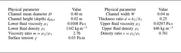

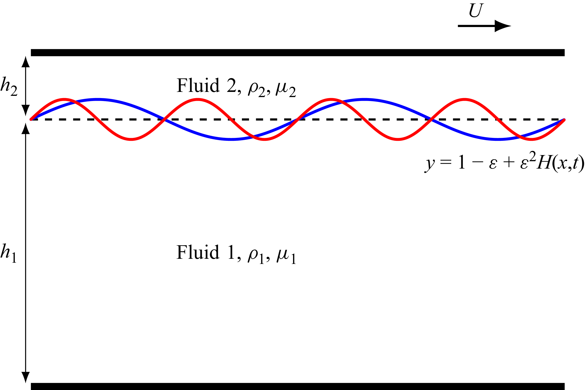


 Open access