





1. Introduction
Vortices are masses of fluid in rotation and are key dynamical features in the oceans (Carton Reference Carton2001), at the surface (Chelton, Schlax & Samelson Reference Chelton, Schlax and Samelson2011) and in the interior (e.g. Petersen et al. Reference Petersen, Williams, Maltrud, Hecht and Hamann2013). Among these, ‘mesoscale vortices’ are those whose horizontal size is comparable to the Rossby deformation radius, of order 20 km. These are among the most energetic features in the oceans (e.g. Grooms, Nadeau & Smith Reference Grooms, Nadeau and Smith2013; Byrne et al. Reference Byrne, Münnich, Frenger and Gruber2016; Hidenori, Xiaoming & Greatbatch Reference Hidenori, Xiaoming and Greatbatch2016). The vortices typically have modest Rossby numbers, so they are amenable to study with a quasi-geostrophic dynamics (Vallis Reference Vallis2006). Vortices interact strongly with their surroundings: with other vortices, with currents and jets, with coasts and with bathymetry. The present paper focuses on the latter. We are specifically interested in mergers between like-signed vortices over isolated features, seamounts and depressions.
Vortex merger is an important elementary interaction. It is associated with the inverse energy and direct enstrophy cascades in large-scale geophysical flows. By merging, vortices form larger structures, contributing in physical space to the inverse energy cascade in spectral space. Mergers also generate filaments (and, occasionally, low-energy, small-scale vortices), contributing to the direct cascade of enstrophy. Vortex merger has thus been the subject of numerous studies. It was first investigated numerically in a two-dimensional incompressible flow by Roberts & Christiansen (Reference Roberts and Christiansen1972) and Rossow (Reference Rossow1977). It was shown that vortices merge provided they are closer than a critical distance. Overman & Zabusky (Reference Overman and Zabusky1982) demonstrated that the merger of two co-rotating patches of uniform vorticity in mutual equilibrium can be linked to an instability of the co-rotating vortex pair, as suggested by Saffman & Szeto (Reference Saffman and Szeto1980) (see also Dritschel Reference Dritschel1995). Mergers in viscous two-dimensional flows have been studied (Meunier et al. Reference Meunier, Ehrenstein, Leweke and Rossi2002; Cerretelli & Williams Reference Cerretelli and Williams2003), as have mergers in quasi-geostrophic, two-layer models (e.g. Polvani, Zabusky & Flierl Reference Polvani, Zabusky and Flierl1989), with the so-called ‘surface quasi-geostrophic’ model (Carton et al. Reference Carton, Ciani, Verron, Reinaud and Sokolvskiy2016), and in three-dimensional, continuously stratified, quasi-geostrophic flow (von Hardenberg et al. Reference von Hardenberg, McWilliams, Provenzale, Shchpetkin and Weiss2000; Dritschel Reference Dritschel2002; Reinaud & Dritschel Reference Reinaud and Dritschel2005; Bambrey, Reinaud & Dritschel Reference Bambrey, Reinaud and Dritschel2007; Ozurgurlu, Reinaud & Dritschel Reference Ozurgurlu, Reinaud and Dritschel2008). Mergers have also studied with finite Froude and Rossby numbers, where an asymmetry between the merger of cyclonic and anticyclonic vortices is observed (Reinaud & Dritschel Reference Reinaud and Dritschel2018). An external shear facilitates mergers between like-signed vortices and impedes mergers otherwise (Carton, Maze & Legras Reference Carton, Maze and Legras2002; Trieling, Dam & van Heijst Reference Trieling, Dam and van Heijst2010; Reinaud Reference Reinaud2017). Mergers over a planar bathymetric slope have also been studied in single (Carton et al. Reference Carton, Morvan, Reinaud, Sokolovskiy, L’Hégaret and Vic2017) and two-layer flows (de Marez et al. Reference de Marez, Carton, Morvan and Reinaud2017).
Bathymetry has significant effects on vortices, see e.g. Zavala Sansón & Gonzalez (Reference Zavala Sansón and Gonzalez2021). An axisymmetric seamount can stabilise a surface cyclone and destabilise an anticyclone, and the opposite occurs over a depression (Benilov Reference Benilov2005; Zhao, Chieusse-Gérard & Flierl Reference Zhao, Chieusse-Gérard and Flierl2019; Gonzalez & Zavala Sansón Reference Gonzalez and Zavala Sansón2023). Isolated cyclones can self-propel up a seamount while anticyclones move off (Carnevale et al. Reference Carnevale, Kloosterziel and Van Heijst1991a ). Turbulent flow over bathymetry can produce mean flows which are ‘prograde’, i.e. parallel to the direction of topographic wave propagation: cyclonic in a basin and anticyclonic over a seamount (Bretherton & Haidvogel Reference Bretherton and Haidvogel1976; Salmon, Holloway & Hendershott Reference Salmon, Holloway and Hendershott1976). With stratification, the flow is bottom intensified, with larger vertical extent for bathymetric features larger than the deformation scale (Hogg Reference Hogg1973; Merryfield Reference Merryfield1998; Venaille Reference Venaille2012; LaCasce, Palóczy & Trodahl Reference LaCasce, Palóczy and Trodahl2024). With a turbulent, barotropic initial state, the result is often a topography-following prograde flow plus an isolated and oppositely signed vortex in the centre (Solodoch, Stewart & McWilliams Reference Solodoch, Stewart and McWilliams2021; Siegelman & Young Reference Siegelman and Young2023). With stratification, one can obtain a bottom-intensified prograde flow and an opposite-signed vortex at the surface (de Marez, Le Corre & Gula Reference de Marez, Le Corre and Gula2021; LaCasce et al. Reference LaCasce, Palóczy and Trodahl2024). The lone vortex is evidently the result of an asymmetry in mergers.
The present goal is to investigate this merger asymmetry. We examine the evolution of two displaced vortices over axisymmetric basins and seamounts (hereafter referred to as circular basins and seamounts) and elliptical basins and seamounts. The results confirm that the merger of cyclones/anticyclones is favoured over a seamount/basin, while the opposite-signed vortices are sheared out. The asymmetry is intimately linked to surface vortex stability, in line with Benilov (Reference Benilov2005) and Zhao et al. (Reference Zhao, Chieusse-Gérard and Flierl2019).
The paper is organised as follows. Section 2 introduces the equations, initial conditions and numerical method. Section 3 presents the main results. The results are analysed in terms of potential vorticity (PV) anomalies induced in the lower layer, and of the stability of a single vortex. We then consider various effects, including (i) basin asymmetry, (ii) vortex scale relative to the deformation radius, (iii) the alignment of vortices and bathymetry and (iv) the initial flow in the lower layer. Conclusions are presented in § 4.
2. Methods
We consider a quasi-geostrophic (QG) two-layer flow over bathymetry. The bathymetric height is denoted $h_b(x,y)$
. We assume the Coriolis frequency is constant,
$h_b(x,y)$
. We assume the Coriolis frequency is constant, $f=f_0$
, for simplicity. The QG flow is fully described by the PVs,
$f=f_0$
, for simplicity. The QG flow is fully described by the PVs, $q_i(x,y,t)$
, in each layer
$q_i(x,y,t)$
, in each layer $i=1,2$
; these are defined from the streamfunction,
$i=1,2$
; these are defined from the streamfunction, $\varphi _i$
,
$\varphi _i$
, $i=1,2$
as
$i=1,2$
as
 \begin{align} q_1 = {\nabla }^2 \varphi _1 - \gamma _1^2 \, (\varphi _1-\varphi _2), \end{align}
 \begin{align} q_2 = {\nabla }^2 \varphi _2 - \gamma _2^2\, (\varphi _2-\varphi _1) + \alpha _b \, h_b; \end{align}
(Vallis Reference Vallis2006). We make the ‘rigid lid’ assumption and neglect deflections of the sea’s surface, which play a minor role at these scales. Layer $i=1$
corresponds to the upper layer while
$i=1$
corresponds to the upper layer while $i=2$
to the bottom layer. The bathymetry lies fully in layer 2. Furthermore,
$i=2$
to the bottom layer. The bathymetry lies fully in layer 2. Furthermore, ${\nabla }^2 = \partial ^2/\partial x^2 + \partial ^2/\partial y^2$
is the horizontal Laplacian, and
${\nabla }^2 = \partial ^2/\partial x^2 + \partial ^2/\partial y^2$
is the horizontal Laplacian, and
 \begin{align} \gamma _i = \dfrac {f_0}{\sqrt {g^{\prime}H_i}} \qquad \alpha _b = \dfrac {f_0}{H_2}, \end{align}
where $H_i$
is the mean depth of layer
$H_i$
is the mean depth of layer $i$
and
$i$
and $g^{\prime}\equiv g\Delta \rho /\rho _0$
is the reduced gravity, with
$g^{\prime}\equiv g\Delta \rho /\rho _0$
is the reduced gravity, with $\Delta \rho \equiv \rho _2-\rho _1$
the density difference between the two layers and
$\Delta \rho \equiv \rho _2-\rho _1$
the density difference between the two layers and $\rho _0= (\rho _1+\rho _2)/2$
the mean density. For simplicity we set
$\rho _0= (\rho _1+\rho _2)/2$
the mean density. For simplicity we set $H_1=H_2=H$
, hence
$H_1=H_2=H$
, hence $\gamma _1=\gamma _2=\gamma \equiv R_d^{-1}$
, where
$\gamma _1=\gamma _2=\gamma \equiv R_d^{-1}$
, where $R_d$
is the Rossby deformation radius. The advecting geostrophic velocity field derives from the streamfunction
$R_d$
is the Rossby deformation radius. The advecting geostrophic velocity field derives from the streamfunction $\varphi _i$
 \begin{equation} (u_i,v_i) = \left (-\dfrac {\partial \varphi _i}{\partial y},\dfrac {\partial \varphi _i}{\partial x}\right)\!, \quad i=1,2. \end{equation}
In the absence of frictional and dissipative effects, the PVs are materially conserved on the $f$
-plane
$f$
-plane
 \begin{align} \dfrac {\mathrm{D} q_1}{\mathrm{D} t} = 0, \nonumber \\[3pt] \dfrac {\mathrm{D} q_2}{\mathrm{D} t}= 0. \end{align}
In layer 2, we also define the PV anomaly
 \begin{equation} q_2^a \equiv q_2-\alpha _b h_b = {\nabla }^2 \varphi _2 - \gamma ^2\, (\varphi _2-\varphi _1). \end{equation}
The PV anomaly $q_2^a$
is not materially conserved. For simplicity we hereafter refer to the fields
$q_2^a$
is not materially conserved. For simplicity we hereafter refer to the fields $q_1$
and
$q_1$
and $q_2^a$
as PV anomalies.
$q_2^a$
as PV anomalies.
We solve the equations numerically using a pseudo-spectral method. Some details are provided in Appendix A. Equations (2.5) are advanced in time using a second-order, semi-implicit, leapfrog integration scheme. For numerical stability, weak bi-harmonic diffusion is added to the right-hand size of (2.5), with a hyperviscosity coefficient $\nu =2\times 10^{-9}$
. The time step is
$\nu =2\times 10^{-9}$
. The time step is $\Delta t= K \, 2\pi / ({\textit{Nu}}_{\textit{max}})$
, where we use a Courant-Friedrichs-Lewy (CFL) coefficient of
$\Delta t= K \, 2\pi / ({\textit{Nu}}_{\textit{max}})$
, where we use a Courant-Friedrichs-Lewy (CFL) coefficient of $K=0.1$
for higher accuracy, where
$K=0.1$
for higher accuracy, where $u_{\textit{max}}$
is the maximum velocity at
$u_{\textit{max}}$
is the maximum velocity at $t=0$
. This choice of
$t=0$
. This choice of $K$
also proved, in practice, to provide numerical stability to the leapfrog scheme. Fields in spectral space are dealiased using the 2/3-rule. A note on numerical convergence is provided in Appendix A.
$K$
also proved, in practice, to provide numerical stability to the leapfrog scheme. Fields in spectral space are dealiased using the 2/3-rule. A note on numerical convergence is provided in Appendix A.
By the symmetry of the QG equations on the $f$
-plane, the evolution of cyclonic vortices over a seamount (or a basin) is equivalent to that of anticyclonic vortices over a basin (or a seamount). We therefore restrict our attention to cyclonic vortices in the upper layer and consider both a basin and a seamount. The initial conditions are given by
$f$
-plane, the evolution of cyclonic vortices over a seamount (or a basin) is equivalent to that of anticyclonic vortices over a basin (or a seamount). We therefore restrict our attention to cyclonic vortices in the upper layer and consider both a basin and a seamount. The initial conditions are given by
 \begin{align} q_1(x,y,0) = q_0\, \mathrm{e}^{-8 \left (\frac {(x-x_{c,1})^2+(y-y_{c,1})^2}{R_v^2}\right)^8} + q_0 \, \mathrm{e}^{-8 \left (\frac {(x-x_{c,2})^2+(y-y_{c,2})^2}{R_v^2}\right)^8}, \end{align}
 \begin{align} q_2^a(x,y,0) = 0, \end{align}
 \begin{align} h_b(x,y) = h_0 \mathrm{e}^{-(x/d_x)^2-(y/d_y)^2}, \\[6pt] \nonumber \end{align}
where $(x_{c,j},y_{c,j})$
is the centre of vortex
$(x_{c,j},y_{c,j})$
is the centre of vortex $j$
at
$j$
at $t=0$
,
$t=0$
, $R_v$
is the common characteristic radius of the two vortices in the upper layer and
$R_v$
is the common characteristic radius of the two vortices in the upper layer and $q_0$
is their common maximum PV. Although the details of the interaction between two vortices depend on their initial shape and their PV distribution, circular vortices are representative of generic vortices and allow investigation of the influence of bathymetry on vortex mergers. We set
$q_0$
is their common maximum PV. Although the details of the interaction between two vortices depend on their initial shape and their PV distribution, circular vortices are representative of generic vortices and allow investigation of the influence of bathymetry on vortex mergers. We set $q_0=1$
. This sets the problem time scale. For example, in the limit
$q_0=1$
. This sets the problem time scale. For example, in the limit $\gamma \to 0$
, a uniform PV axisymmetric vortex has a turnover period of
$\gamma \to 0$
, a uniform PV axisymmetric vortex has a turnover period of $T=4\pi /q_0 = 4\pi$
. The bathymetry consists of a single elliptical Gaussian seamount/basin of length
$T=4\pi /q_0 = 4\pi$
. The bathymetry consists of a single elliptical Gaussian seamount/basin of length $d_x$
in the
$d_x$
in the $x$
-direction and
$x$
-direction and $d_y$
in the
$d_y$
in the $y$
-direction, and maximal height
$y$
-direction, and maximal height $h_0$
. Circular bathymetry has
$h_0$
. Circular bathymetry has $d_x=d_y$
. The topographic height is varied, but we use
$d_x=d_y$
. The topographic height is varied, but we use $h_0=\pm 1=\alpha _b^{-1}$
for a seamount and basin, respectively, such that
$h_0=\pm 1=\alpha _b^{-1}$
for a seamount and basin, respectively, such that $\alpha _b h_0 = \pm q_0$
unless stated otherwise. The initial vortex spacing is
$\alpha _b h_0 = \pm q_0$
unless stated otherwise. The initial vortex spacing is $\Delta R \equiv \sqrt {(x_{c,2}-x_{c,1})^2 + (y_{c,2}-y_{c,1})^2 }$
.
$\Delta R \equiv \sqrt {(x_{c,2}-x_{c,1})^2 + (y_{c,2}-y_{c,1})^2 }$
.
The vortex radius is $R_v=R_d$
, unless stated otherwise. The vortices are, however, always kept small compared with the domain, to limit the effects of the periodic boundary conditions in the horizontal directions. Note too that, despite the vortex PV distributions being physically separate, the streamfunctions overlap; thus the vortices interact. Figure 1 illustrates the geometry of the initial condition for a circular seamount with
$R_v=R_d$
, unless stated otherwise. The vortices are, however, always kept small compared with the domain, to limit the effects of the periodic boundary conditions in the horizontal directions. Note too that, despite the vortex PV distributions being physically separate, the streamfunctions overlap; thus the vortices interact. Figure 1 illustrates the geometry of the initial condition for a circular seamount with $d_x=d_y=R_b=3R_d$
.
$d_x=d_y=R_b=3R_d$
.
Geometry of the initial conditions. Bathymetry (Gaussian seamount) of characteristic radius $h_b(x,y)$
with
$h_b(x,y)$
with $R_b=3R_d=1$
(black). The PV field in the upper layer
$R_b=3R_d=1$
(black). The PV field in the upper layer $q_1$
at
$q_1$
at $t=0$
for
$t=0$
for $R_v=R_d$
and
$R_v=R_d$
and $\Delta R=3R_d$
(red).
$\Delta R=3R_d$
(red).

The problem has four non-dimensional parameters: the initial distance between the two vortices, the vortex radius, the bathymetry characteristic radius and the bathymetry height. The main focus of the paper is on the effect of the first two parameters. We also conduct additional numerical experiments to explore the effects of the radius and height of the bathymetry.
3. Results
3.1. Circular bathymetry
We first consider a circular seamount/basin with $d_x=d_y=R_b=3R_d$
. We define a global topographic beta,
$d_x=d_y=R_b=3R_d$
. We define a global topographic beta, $\beta _t = f_0h_0/(R_b H) = \alpha _bh_0/R_b=\pm 1$
for the seamount/basin. The vortex radius is set to the Rossby deformation radius so that
$\beta _t = f_0h_0/(R_b H) = \alpha _bh_0/R_b=\pm 1$
for the seamount/basin. The vortex radius is set to the Rossby deformation radius so that $R_v=R_d$
, and the initial spacing is
$R_v=R_d$
, and the initial spacing is $\Delta R=2R_v$
at
$\Delta R=2R_v$
at $t=0$
.
$t=0$
.
Figure 2 shows the PV anomalies $q_1$
and
$q_1$
and $q_2^a$
at
$q_2^a$
at $t=250$
for a basin (panels a and d), a flat bottom (b and e) and a seamount (c and f). With the flat bottom,
$t=250$
for a basin (panels a and d), a flat bottom (b and e) and a seamount (c and f). With the flat bottom, $q_2^a$
remains zero, as expected. In all three cases, the vortices in the upper layer merge. With the flat bottom or seamount, the merged vortices shed a small amount of filamentary PV. But with the basin, the vortices have been almost completely strained out. What remains is an intricate pattern of filamentary PV and two small PV cores. At the same time, the lower-layer PV anomaly,
$q_2^a$
remains zero, as expected. In all three cases, the vortices in the upper layer merge. With the flat bottom or seamount, the merged vortices shed a small amount of filamentary PV. But with the basin, the vortices have been almost completely strained out. What remains is an intricate pattern of filamentary PV and two small PV cores. At the same time, the lower-layer PV anomaly, $q_2^a$
, has organised into a tripole, with cyclonic PV at the basin centre and anticyclonic vortices on the side. The vortices have strong associated surface flows and these stir the surface PV. A similar erosion of an anticyclonic vortex over a seamount was described by Herbette, Morel & Arhan (Reference Herbette, Morel and Arhan2003). Finally, the
$q_2^a$
, has organised into a tripole, with cyclonic PV at the basin centre and anticyclonic vortices on the side. The vortices have strong associated surface flows and these stir the surface PV. A similar erosion of an anticyclonic vortex over a seamount was described by Herbette, Morel & Arhan (Reference Herbette, Morel and Arhan2003). Finally, the $q_2^a$
-pattern observed in figure 2(f) resembles one of the linear trapped Rossby waves obtained by Zavala Sansón (Reference Zavala Sansón2010).
$q_2^a$
-pattern observed in figure 2(f) resembles one of the linear trapped Rossby waves obtained by Zavala Sansón (Reference Zavala Sansón2010).
Potential vorticity anomalies at $t=250$
for deformation-scale vortices (
$t=250$
for deformation-scale vortices ( $R_v=R_d$
) with an initial separation of
$R_v=R_d$
) with an initial separation of $\Delta R=2R_v$
. Top row:
$\Delta R=2R_v$
. Top row: $q_1$
for (a) a flat bathymetry, (b) a circular basin and (c) a circular seamount. Bottom row:
$q_1$
for (a) a flat bathymetry, (b) a circular basin and (c) a circular seamount. Bottom row: $q_2^a$
for (d) a flat bathymetry, (e) a circular basin and (f) a circular seamount.
$q_2^a$
for (d) a flat bathymetry, (e) a circular basin and (f) a circular seamount.

The evolution of the maximum and minimum PV anomalies at depth, i.e. $|q_{2,m}^-| = |{\textit{min}}_{\textit{domain}} q_{2}^a|$
and
$|q_{2,m}^-| = |{\textit{min}}_{\textit{domain}} q_{2}^a|$
and $q_{2,m}^+={\textit{max}}_{\textit{domain}} q_2^a$
, are shown in panel (a) of figure 3 for the basin and seamount cases. The initial increase in both cases is similar. Over the seamount, the maximum plateaus to a value 6.6 % times the surface maximum,
$q_{2,m}^+={\textit{max}}_{\textit{domain}} q_2^a$
, are shown in panel (a) of figure 3 for the basin and seamount cases. The initial increase in both cases is similar. Over the seamount, the maximum plateaus to a value 6.6 % times the surface maximum, $q_0$
, but over the basin, the values increase much more, to approximately
$q_0$
, but over the basin, the values increase much more, to approximately ${\sim}47\,\%$
of
${\sim}47\,\%$
of $q_0$
, reflecting the formation of the deep tripole.
$q_0$
, reflecting the formation of the deep tripole.
Evolution of (a) the maximal PV anomaly in the bottom layer (in absolute value) $|q_{2,m}^-|$
(solid lines) and
$|q_{2,m}^-|$
(solid lines) and $q_{2,m}^+$
(dotted lines) for
$q_{2,m}^+$
(dotted lines) for $R_v=R_d$
and
$R_v=R_d$
and $\Delta R=2R_v$
, for a basin (black) and a seamount (red); (b) surface circulation,
$\Delta R=2R_v$
, for a basin (black) and a seamount (red); (b) surface circulation, $\varGamma _m$
, of the PV anomaly
$\varGamma _m$
, of the PV anomaly $q_1$
of the largest vortex over the total circulation of all vortices
$q_1$
of the largest vortex over the total circulation of all vortices $\varGamma _{tot}$
for a circular basin (black), a circular seamount (red) and a flat bottom (blue); (c) distance between the centres of the two largest vortices of the upper layer (same colours as in panel (b)); (d) trajectory of the vortex centres (same colours as in panel (b) and the circles denote the initial vortex centre locations).
$\varGamma _{tot}$
for a circular basin (black), a circular seamount (red) and a flat bottom (blue); (c) distance between the centres of the two largest vortices of the upper layer (same colours as in panel (b)); (d) trajectory of the vortex centres (same colours as in panel (b) and the circles denote the initial vortex centre locations).

Shown in figure 3(b) is the integrated surface PV anomaly of the largest coherent structure divided by the sum of the same quantity over all structures in the upper layer, denoted $\varGamma _m$
. A coherent structure is defined as a region of contiguous PV in excess of the root-mean-square value over the computational domain. A unit value of
$\varGamma _m$
. A coherent structure is defined as a region of contiguous PV in excess of the root-mean-square value over the computational domain. A unit value of $\varGamma _m$
indicates there is only one coherent structure present. At
$\varGamma _m$
indicates there is only one coherent structure present. At $t=0$
,
$t=0$
, $\varGamma _m=0.5$
as there are two identical vortices in the upper layer. As the vortices merge,
$\varGamma _m=0.5$
as there are two identical vortices in the upper layer. As the vortices merge, $\varGamma _m \rightarrow 1$
. The figure shows the vortices merge very rapidly, by
$\varGamma _m \rightarrow 1$
. The figure shows the vortices merge very rapidly, by $t\simeq 5$
, in all three cases (basin, flat bathymetry, seamount). From time to time, filaments detach from the main vortex, causing
$t\simeq 5$
, in all three cases (basin, flat bathymetry, seamount). From time to time, filaments detach from the main vortex, causing $\varGamma _m$
to decrease below one; but it returns to one as the filaments are either reabsorbed or dissipated. Note
$\varGamma _m$
to decrease below one; but it returns to one as the filaments are either reabsorbed or dissipated. Note $\varGamma _m \simeq 1$
at
$\varGamma _m \simeq 1$
at $t=250$
also for the basin; thus the mixture of filaments and small vortices by this measure is like a highly deformed single structure.
$t=250$
also for the basin; thus the mixture of filaments and small vortices by this measure is like a highly deformed single structure.
Having identified the coherent structures, we can determine their geometric centres. Figure 3(c) shows the evolution of the distance between the two vortex centres until they merge at $t\simeq 4$
. The results indicate the merger is faster/slower over the seamount/basin than over a flat bottom. Panel (d) shows the trajectory of the centres in the upper layer until they merge. These are visually indistinguishable in the three cases.
$t\simeq 4$
. The results indicate the merger is faster/slower over the seamount/basin than over a flat bottom. Panel (d) shows the trajectory of the centres in the upper layer until they merge. These are visually indistinguishable in the three cases.
The early evolution of the PV for the basin is shown in figure 4 while figure 5 shows the same fields over the seamount. In both cases, $q_2^a$
exhibits a quadrupole structure initially, i.e. azimuthal mode
$q_2^a$
exhibits a quadrupole structure initially, i.e. azimuthal mode $m=2$
. The pattern is reminiscent of seamount-trapped waves (Brink Reference Brink1990; Haidvogel et al. Reference Haidvogel, Beckmann, Chapman and Lin1993), but the propagation direction differs, being counter-clockwise over both bathymetries. Shortly thereafter the evolutions differ. Over the basin, the cyclonic lobes merge and settle in the basin centre while the anticyclonic lobes circle as satellites, and the resulting tripole intensifies. With the seamount this never happens; instead, the deep quadrupole strains out and fails to intensify.
$m=2$
. The pattern is reminiscent of seamount-trapped waves (Brink Reference Brink1990; Haidvogel et al. Reference Haidvogel, Beckmann, Chapman and Lin1993), but the propagation direction differs, being counter-clockwise over both bathymetries. Shortly thereafter the evolutions differ. Over the basin, the cyclonic lobes merge and settle in the basin centre while the anticyclonic lobes circle as satellites, and the resulting tripole intensifies. With the seamount this never happens; instead, the deep quadrupole strains out and fails to intensify.
Potential vorticity anomalies for the circular basin case at earlier times, with $R_v=R_d$
and
$R_v=R_d$
and $\Delta R=2R_v$
. Top row:
$\Delta R=2R_v$
. Top row: $q_1$
at (a)
$q_1$
at (a) $t=12$
, (b)
$t=12$
, (b) $t=62$
and (c)
$t=62$
and (c) $t=100$
. Bottom row:
$t=100$
. Bottom row: $q_2^a$
at (d)
$q_2^a$
at (d) $t=12$
, (e)
$t=12$
, (e) $t=62$
and (f)
$t=62$
and (f) $t=100$
.
$t=100$
.

Potential vorticity anomalies for the circular seamount at earlier times, with $R_v=R_d$
and
$R_v=R_d$
and $\Delta R=2R_v$
. Top row
$\Delta R=2R_v$
. Top row $q_1$
at (a)
$q_1$
at (a) $t=12$
, (b)
$t=12$
, (b) $t=62$
and (c)
$t=62$
and (c) $t=100$
. Bottom row
$t=100$
. Bottom row $q_2^a$
at (d)
$q_2^a$
at (d) $t=12$
, (e)
$t=12$
, (e) $t=62$
and (f)
$t=62$
and (f) $t=100$
.
$t=100$
.

The deep tripole has no expression in the surface PV (as seen by the two blank regions in surface PV in figure 4(b,c). This is as expected for topographic waves in two layers (LaCasce Reference LaCasce1998; LaCasce et al. Reference LaCasce, Palóczy and Trodahl2024). However, the features do have surface flow, and the strength of topographic wave surface flow depends on the wavelength; if comparable to the deformation radius (as here), the flow approaches the bottom flow in strength. The result is a strong interaction between the deep and surface anomalies. The effect is absent over the seamount on the other hand. The merged vortex persists, gradually becoming more axisymmetric.
Figure 6 shows the same PV diagnostics as in figure 3 but with a greater initial vortex separation ( $\Delta R=3R_v$
). Here, differences over the three types of bathymetry are even more pronounced. While the surface vortices merge over the seamount (red curves in panels c and d), the vortices over a flat bottom and basin co-rotate without merging (blue and black curves). Indeed, in the latter case the vortices slowly migrate away from each other. The fraction of PV in a single structure thus reaches one for the seamount but stays near 0.5 for the other cases (panel b). However, as before, the formation of deep PV anomalies is most pronounced over the basin (black curves in panel a); it is weaker over the seamount (red curves).
$\Delta R=3R_v$
). Here, differences over the three types of bathymetry are even more pronounced. While the surface vortices merge over the seamount (red curves in panels c and d), the vortices over a flat bottom and basin co-rotate without merging (blue and black curves). Indeed, in the latter case the vortices slowly migrate away from each other. The fraction of PV in a single structure thus reaches one for the seamount but stays near 0.5 for the other cases (panel b). However, as before, the formation of deep PV anomalies is most pronounced over the basin (black curves in panel a); it is weaker over the seamount (red curves).
Evolution of (a) the maximal PV anomaly in the bottom layer (in absolute value) $|q_{2,m}^-|$
and
$|q_{2,m}^-|$
and $q_{2,m}^+$
for
$q_{2,m}^+$
for $R_v=R_d$
,
$R_v=R_d$
, $\Delta R=3R_v$
, with a circular basin (black) and a circular seamount (red); (b) surface circulation,
$\Delta R=3R_v$
, with a circular basin (black) and a circular seamount (red); (b) surface circulation, $\varGamma _m$
, of
$\varGamma _m$
, of $q_1$
of the largest vortex over the total circulation of all vortices
$q_1$
of the largest vortex over the total circulation of all vortices $\varGamma _{tot}$
for a basin (black), a seamount (red) and a flat bathymetry (blue); (c) distance between the centres of the two largest vortices of the upper layer (same colours as in panel (b)); (d) trajectory of the vortex centres (same colours as in panel (b) and the circles denote the initial vortex centre locations).
$\varGamma _{tot}$
for a basin (black), a seamount (red) and a flat bathymetry (blue); (c) distance between the centres of the two largest vortices of the upper layer (same colours as in panel (b)); (d) trajectory of the vortex centres (same colours as in panel (b) and the circles denote the initial vortex centre locations).

Qualitative descriptions of the evolution of the pair of cyclonic vortices in the upper layer for $ R_v=R_d$
over a circular bathymetry for
$ R_v=R_d$
over a circular bathymetry for $0\leqslant t \leqslant 250$
.
$0\leqslant t \leqslant 250$
.

The behaviour for a range of initial separations, $\Delta R$
, is summarised in table 1 and illustrated in figure 7. Most significantly, the vortices must be closer than approximately
$\Delta R$
, is summarised in table 1 and illustrated in figure 7. Most significantly, the vortices must be closer than approximately $2.6 R_v$
to merge over a basin while they can be as far apart as
$2.6 R_v$
to merge over a basin while they can be as far apart as $3.2 R_v$
above a seamount. For reference, the critical merger distance is
$3.2 R_v$
above a seamount. For reference, the critical merger distance is $2.7R_v$
over a flat bottom. Moreover, the core of the merged vortex is much smaller over a basin than over a seamount, again as a large part of the PV is strained out into filaments.
$2.7R_v$
over a flat bottom. Moreover, the core of the merged vortex is much smaller over a basin than over a seamount, again as a large part of the PV is strained out into filaments.
Evolution of the relative distance, $d\!/\!R_v$
, between the centres of the upper-layer vortices with
$d\!/\!R_v$
, between the centres of the upper-layer vortices with $R_v=R_d$
until they first touch for (a) a circular basin and
$R_v=R_d$
until they first touch for (a) a circular basin and $\Delta R\!/\!R_v=2.55$
(black),
$\Delta R\!/\!R_v=2.55$
(black), $2.6$
(red),
$2.6$
(red), $2.7$
(blue),
$2.7$
(blue), $2.8$
(green),
$2.8$
(green), $2.9$
(cyan) and
$2.9$
(cyan) and $2.95$
(magenta); (b) a flat bathymetry and
$2.95$
(magenta); (b) a flat bathymetry and $\Delta R\!/\!R_v=2.7$
(black),
$\Delta R\!/\!R_v=2.7$
(black), $2.75$
(red),
$2.75$
(red), $2.8$
(blue),
$2.8$
(blue), $2.9$
(green),
$2.9$
(green), $2.95$
(cyan); (c) a circular seamount and
$2.95$
(cyan); (c) a circular seamount and $\Delta R\!/\!R_v=3$
(black),
$\Delta R\!/\!R_v=3$
(black), $3.05$
(red),
$3.05$
(red), $3.1$
(blue),
$3.1$
(blue), $3.2$
(green),
$3.2$
(green), $3.3$
(cyan),
$3.3$
(cyan), $3.4$
(magenta) and
$3.4$
(magenta) and $3.45$
(yellow). In panels (a–c) a circle indicates merger and a cross a weaker interaction not leading to merger. Panels (d–f) show trajectories of the vortex centres for a basin and a flat bottom and a seamount, respectively, using the same colour code as panels (a–c). The small circles indicate the initial locations of the centres.
$3.45$
(yellow). In panels (a–c) a circle indicates merger and a cross a weaker interaction not leading to merger. Panels (d–f) show trajectories of the vortex centres for a basin and a flat bottom and a seamount, respectively, using the same colour code as panels (a–c). The small circles indicate the initial locations of the centres.

3.2.
Initial production of $q_2^a$

The generation of the deep anomalies initially can be estimated analytically. To do this, we represent the vortices as two circular regions with uniform PV. We define the barotropic PV, $q_b$
, and the baroclinic PV,
$q_b$
, and the baroclinic PV, $q_c$
, such that
$q_c$
, such that
 \begin{equation} q_b=\dfrac {q_1+q_2^a}{2}, \qquad q_c=\dfrac {q_1-q_2^a}{2}. \end{equation}
The associated barotropic and baroclinic streamfunctions are $\varphi _b$
and
$\varphi _b$
and $\varphi _c$
, such that
$\varphi _c$
, such that
 \begin{equation} q_b = {\nabla }^2 \varphi _b, \qquad q_c = {\nabla }^2 \varphi _c - \gamma ^{*2}\varphi _c, \end{equation}
where $\gamma ^*=\sqrt {2}\gamma _1= \sqrt {2}\gamma _2$
, with equal layer depths.
$\gamma ^*=\sqrt {2}\gamma _1= \sqrt {2}\gamma _2$
, with equal layer depths.
For a single patch of radius $R_v$
of uniform PV
$R_v$
of uniform PV $q_0$
at
$q_0$
at $(0,0)$
, (3.2) can be inverted to give
$(0,0)$
, (3.2) can be inverted to give
 \begin{gather} \varphi _b = \begin{cases} \dfrac {q_br^2}{4}, & r\leqslant R_v, \\[8pt] \dfrac {q_b R_v}{2}\ln (r\!/\!R_v)+ \dfrac {q_b}{4}, & r\gt R_v, \end{cases} \end{gather}
 \begin{gather} \varphi _c = \begin{cases} \dfrac {q_c}{\gamma ^{*2}} \left (\gamma ^*R_v {K}_{\!1}(\gamma ^*R_v){I}_0(\gamma ^*r)-1\right)\!, & r\leqslant R_v, \\[10pt] \dfrac {q_c}{\gamma ^{*2}} \left (-\gamma ^*R_v {K}_0(\gamma ^*r) I_1(\gamma ^*R_v)\right)\!,& r\gt R_v, \end{cases} \end{gather}
where ${K}_0$
and
${K}_0$
and ${K}_1$
are the modified Bessel functions of the second kind for zeroth and first orders, while
${K}_1$
are the modified Bessel functions of the second kind for zeroth and first orders, while ${I}_0$
and
${I}_0$
and ${I}_1$
are the modified Bessel functions of the first kind of zeroth and first orders (e.g. Sokolovskiy & Verron Reference Sokolovskiy and Verron2014). The associated azimuthal barotropic and baroclinic azimuthal velocities are
${I}_1$
are the modified Bessel functions of the first kind of zeroth and first orders (e.g. Sokolovskiy & Verron Reference Sokolovskiy and Verron2014). The associated azimuthal barotropic and baroclinic azimuthal velocities are
 \begin{gather} u_b = \begin{cases} \dfrac {q_b r}{2}, & r\leqslant R_v, \\[8pt] \dfrac {q_b R_v^2}{2r}, & r\gt R_v, \end{cases} \end{gather}
 \begin{gather} u_c = \begin{cases} q_c R_v {K}_1(\gamma ^* R_v) {I}_1(\gamma ^* r), & r\leqslant R_v, \\ q_c R_v {K}_1(\gamma ^* r) {I}_1(\gamma ^* R_v), & r\gt R_v. \end{cases} \end{gather}
Then, the flow azimuthal velocity induced in the lower layer by the surface vortex is $\boldsymbol{u}_2=u_2\boldsymbol{e}_\theta$
, where
$\boldsymbol{u}_2=u_2\boldsymbol{e}_\theta$
, where
 \begin{equation} u_2 = u_c-u_b = \begin{cases} \dfrac {q_0 }{2} \left ( \dfrac {r}{2}-R_v {K}_1(\gamma ^* R_v) {I}_1(\gamma ^* r)\right)\!, & r\leqslant R_v, \\[8pt] \dfrac {q_0}{2} \left ( \dfrac {R_v^2}{2r} - R_v {K}_1(\gamma ^* r) {I}_1(\gamma ^* R_v) \right)\!, & r\gt R_v, \end{cases} \end{equation}
where $\boldsymbol{e}_\theta$
is the azimuthal unit vector and we have used
$\boldsymbol{e}_\theta$
is the azimuthal unit vector and we have used $q_b=q_c=q_0/2$
. By linearity of the equations, the velocity
$q_b=q_c=q_0/2$
. By linearity of the equations, the velocity $\boldsymbol{u}_2$
induced by two identical circular patches of radius
$\boldsymbol{u}_2$
induced by two identical circular patches of radius $R_v$
of uniform PV
$R_v$
of uniform PV $q_0$
located at
$q_0$
located at $(\pm d,0)$
is the sum of the velocities induced by each vortex following (3.7) where
$(\pm d,0)$
is the sum of the velocities induced by each vortex following (3.7) where $r$
is replaced by
$r$
is replaced by $r^{\pm } = \sqrt {(x\mp d)^2+y^2}$
and the azimuthal unit vector is defined locally relative to the centre of each vortex. Material conservation of the PV
$r^{\pm } = \sqrt {(x\mp d)^2+y^2}$
and the azimuthal unit vector is defined locally relative to the centre of each vortex. Material conservation of the PV $q_2$
in layer 2 at
$q_2$
in layer 2 at $t=0$
implies that
$t=0$
implies that
 \begin{align} \dfrac {\mathrm{D} q_2}{\mathrm{D} t} &= \dfrac {\partial q_2^a}{\partial t} + \boldsymbol{u} \boldsymbol{\cdot } \boldsymbol{\nabla } (\alpha _b h_b) = 0, \end{align}
 \begin{align} \dfrac {\partial q_2^a}{\partial t} &= 2\alpha _b h_b r\boldsymbol{e}_r \boldsymbol{\cdot } \boldsymbol{u}_2, \end{align}
where $\boldsymbol{e}_r$
is the radial unit vector.
$\boldsymbol{e}_r$
is the radial unit vector.
Figure 9 shows $\partial q_2^a/\partial t$
at
$\partial q_2^a/\partial t$
at $t=0$
using the same parameters as in § 3.1. This confirms the initial quadrupole pattern seen in § 3.1. It also demonstrates the sensitivity of the intensity of
$t=0$
using the same parameters as in § 3.1. This confirms the initial quadrupole pattern seen in § 3.1. It also demonstrates the sensitivity of the intensity of $q_2^a$
to the location of the surface vortices on the slope of the bathymetry.
$q_2^a$
to the location of the surface vortices on the slope of the bathymetry.
Potential vorticity anomalies at $t=250$
for
$t=250$
for $R_v= R_d$
. Top row
$R_v= R_d$
. Top row $q_1$
for (a) a circular basin with
$q_1$
for (a) a circular basin with $\Delta R=2.55$
, (b) a flat bottom with
$\Delta R=2.55$
, (b) a flat bottom with $\Delta R=2.7$
and (c) a circular seamount with
$\Delta R=2.7$
and (c) a circular seamount with $\Delta R=3.0$
. Bottom row,
$\Delta R=3.0$
. Bottom row, $q_2^a$
for (d) a circular basin, (e) flat bottom and (f) a circular seamount.
$q_2^a$
for (d) a circular basin, (e) flat bottom and (f) a circular seamount.

Tendency $\partial q_2^a/\partial t$
at
$\partial q_2^a/\partial t$
at $t=0$
for two uniform circular patches with
$t=0$
for two uniform circular patches with $\Delta R=2R_v,\, 3.33R_v$
and
$\Delta R=2R_v,\, 3.33R_v$
and $4.67R_v$
. The black circles indicate the location of the upper-layer patches. Only the sub-portion of the domain
$4.67R_v$
. The black circles indicate the location of the upper-layer patches. Only the sub-portion of the domain $[-2,2]\times [-2,2]$
is shown.
$[-2,2]\times [-2,2]$
is shown.

3.3. Stability of a single vortex
The merged upper-layer vortex also has different stability properties over the bathymetry, as shown by Benilov (Reference Benilov2005) and Zhao et al. (Reference Zhao, Chieusse-Gérard and Flierl2019). To see this, we consider a single upper-layer vortex over a Gaussian bathymetry. Again, the vortex is assumed to have uniform PV, $q_0$
, and radius
$q_0$
, and radius $R_v$
. We again assume equal layer depths, with
$R_v$
. We again assume equal layer depths, with $\gamma _1=\gamma _2=\gamma$
.
$\gamma _1=\gamma _2=\gamma$
.
The upper vortex is fully described by the radial coordinate of its boundary $r_1(\theta,t)$
, with
$r_1(\theta,t)$
, with $\bar {r}_1=R_v$
the basic state vortex radius. The lower-layer PV, a perturbation on the bathymetric contribution,
$\bar {r}_1=R_v$
the basic state vortex radius. The lower-layer PV, a perturbation on the bathymetric contribution, $q_2=\alpha _0h_b$
, is discretised by
$q_2=\alpha _0h_b$
, is discretised by $N_t$
circular contours of radius
$N_t$
circular contours of radius $\bar {r}_{2,i}$
,
$\bar {r}_{2,i}$
, $1\leqslant i\leqslant N_t$
, corresponding to constant jumps in
$1\leqslant i\leqslant N_t$
, corresponding to constant jumps in $q_2$
.
$q_2$
.
The contours of $q_1$
and
$q_1$
and $q_2$
are then perturbed such that
$q_2$
are then perturbed such that
 \begin{gather} r_1(\theta,t) = \bar {r}_1 + \epsilon {\textrm{Re}} \left (\eta _1(t) \mathrm{e}^{\mathrm{i} (m\theta -\sigma t)}\right)\!, \end{gather}
 \begin{gather} r_{2,i}(\theta,t) = \bar {r}_{2,i} + \epsilon {\textrm{Re}} \left (\eta _{2,i}(t) \mathrm{e}^{\mathrm{i} (m\theta -\sigma t)}\right)\!, \end{gather}
where $m$
is the azimuthal wavenumber of the perturbation and
$m$
is the azimuthal wavenumber of the perturbation and $ \epsilon \eta _1, \epsilon \eta _{2mi}$
are the perturbation complex amplitudes,
$ \epsilon \eta _1, \epsilon \eta _{2mi}$
are the perturbation complex amplitudes, $\sigma =\sigma _r + \mathrm{i} \sigma _i$
is the complex frequency and
$\sigma =\sigma _r + \mathrm{i} \sigma _i$
is the complex frequency and ${\textrm{Re}} (\boldsymbol{\cdot })$
denotes the real part. The imaginary part of
${\textrm{Re}} (\boldsymbol{\cdot })$
denotes the real part. The imaginary part of $\sigma$
is the mode’s growth rate. The linearised equations for the perturbations
$\sigma$
is the mode’s growth rate. The linearised equations for the perturbations $\eta _1, \eta _{2,i}$
yield an eigenvalue problem which we solved numerically. The details of the numerical analysis are given in Appendix B. We set
$\eta _1, \eta _{2,i}$
yield an eigenvalue problem which we solved numerically. The details of the numerical analysis are given in Appendix B. We set $q_0=1$
and
$q_0=1$
and $N_t=8000$
.
$N_t=8000$
.
The maximum growth rate as a function of $R_v$
is plotted in figure 10 for the basin case with
$R_v$
is plotted in figure 10 for the basin case with $\gamma R_v \in [0,5.5]$
. The largest growth rate corresponds to
$\gamma R_v \in [0,5.5]$
. The largest growth rate corresponds to $\sigma _i/q_0=0.0345$
for
$\sigma _i/q_0=0.0345$
for $\gamma \! R_v=1.43$
. There is a ‘short-wave’ cutoff as well, as vortices with
$\gamma \! R_v=1.43$
. There is a ‘short-wave’ cutoff as well, as vortices with $\gamma R_v \lt 1$
are stable. A similar calculation for the same vortex over a seamount indicates it is neutrally stable.
$\gamma R_v \lt 1$
are stable. A similar calculation for the same vortex over a seamount indicates it is neutrally stable.
Normalised maximal growth rate $\sigma _i/q_0$
vs the normalised vortex radius
$\sigma _i/q_0$
vs the normalised vortex radius $\gamma R_v$
for a single uniform PV upper-layer vortex over a Gaussian basin for the perturbation mode of azimuthal wavenumber
$\gamma R_v$
for a single uniform PV upper-layer vortex over a Gaussian basin for the perturbation mode of azimuthal wavenumber $m=2$
.
$m=2$
.

The nonlinear evolution of a single vortex with $R_v=0.467$
(
$R_v=0.467$
( $\gamma R_v=1.4$
) is presented in figure 11. The upper vortex has the same PV profile as defined by (2.8) for the two vortex-merger problem. The vortex has uniform PV, smoothed to avoid Gibbs effects in our pseudo-spectral calculation. Mode
$\gamma R_v=1.4$
) is presented in figure 11. The upper vortex has the same PV profile as defined by (2.8) for the two vortex-merger problem. The vortex has uniform PV, smoothed to avoid Gibbs effects in our pseudo-spectral calculation. Mode $m=2$
is initially excited by making the vortex slightly elliptical, with an aspect ratio of
$m=2$
is initially excited by making the vortex slightly elliptical, with an aspect ratio of $1.01$
. As expected, mode
$1.01$
. As expected, mode $m=2$
is unstable and the perturbation amplifies. The evolution bares a striking resemblance to that of the merged vortex (figure 2); a deep tripole forms and the surface cyclone is destroyed.
$m=2$
is unstable and the perturbation amplifies. The evolution bares a striking resemblance to that of the merged vortex (figure 2); a deep tripole forms and the surface cyclone is destroyed.
Potential vorticity anomalies for a single vortex of radius $R_v=1.4R_d$
over a circular basin. Top row,
$R_v=1.4R_d$
over a circular basin. Top row, $q_1$
at (a)
$q_1$
at (a) $t=0$
, (b)
$t=0$
, (b) $t=150$
and (c)
$t=150$
and (c) $t=300$
. Bottom row,
$t=300$
. Bottom row, $q_2^a$
for (d)
$q_2^a$
for (d) $t=0$
, (e)
$t=0$
, (e) $t=150$
and (f)
$t=150$
and (f) $t=300$
.
$t=300$
.

3.4. Other aspects
3.4.1. Elliptical bathymetry
In turbulent flows, anticyclones trapped over an asymmetric basin are smaller than over a circular one (LaCasce et al. Reference LaCasce, Palóczy and Trodahl2024). We thus consider mergers between surface cyclones over an elliptical basin and an elliptical seamount. We set $d_x/d_y=1.5$
while keeping
$d_x/d_y=1.5$
while keeping $d_xd_y=1$
so that the elliptical basin or seamount covers the same area as the circular ones. Figure 12 shows the PV anomaly in both layers at
$d_xd_y=1$
so that the elliptical basin or seamount covers the same area as the circular ones. Figure 12 shows the PV anomaly in both layers at $t=250$
for both cases, with
$t=250$
for both cases, with $\Delta R=2R_v$
and
$\Delta R=2R_v$
and $R_v=R_d$
. The change in bathymetry from circular to elliptical is reflected in the final PV distributions, which are similarly asymmetric and cover the bathymetry.
$R_v=R_d$
. The change in bathymetry from circular to elliptical is reflected in the final PV distributions, which are similarly asymmetric and cover the bathymetry.
Potential vorticity anomalies at $t=250$
for
$t=250$
for $\Delta R=2R_v$
and
$\Delta R=2R_v$
and $ R_v=R_d$
. Top row,
$ R_v=R_d$
. Top row, $q_1$
for (a) an elliptical basin, (b) an elliptical seamount. Bottom row,
$q_1$
for (a) an elliptical basin, (b) an elliptical seamount. Bottom row, $q_2^a$
for (c) an elliptical basin, (d) an elliptical seamount.
$q_2^a$
for (c) an elliptical basin, (d) an elliptical seamount.

Table 2 summarises results from a suite of experiments. Notably, the vortices now interact from further apart, apparently due to the increase in the bathymetric extent in the $x$
-direction. Over the circular basin, the smallest distance for which the vortices do not interact is
$x$
-direction. Over the circular basin, the smallest distance for which the vortices do not interact is $\Delta R\!/\!R_v=2.95$
while it is
$\Delta R\!/\!R_v=2.95$
while it is $3.5$
for the elliptical basin. The critical separation is larger still for the seamounts,
$3.5$
for the elliptical basin. The critical separation is larger still for the seamounts, $3.45$
for the circular seamount and
$3.45$
for the circular seamount and $4.3$
for the elliptical one.
$4.3$
for the elliptical one.
Qualitative description of the evolution of the pair of cyclonic vortices in the upper layer for $\gamma _1 R_v=\gamma _2 R_v=1$
over an elliptical bathymetry or an elliptical seamount for
$\gamma _1 R_v=\gamma _2 R_v=1$
over an elliptical bathymetry or an elliptical seamount for $0\leqslant t \leqslant 250$
.
$0\leqslant t \leqslant 250$
.

The separation distance $d$
between the vortex centres is plotted in figure 13. The results confirm the vortices interact from further apart when over the elliptical bathymetry. With both a basin and a seamount, the trajectories are more elliptical than in the circular case (panels c, d). The trajectories over the seamount are also more convoluted; this is due to the formation of multipolar structures in the lower layer which act back on the surface vortices.
$d$
between the vortex centres is plotted in figure 13. The results confirm the vortices interact from further apart when over the elliptical bathymetry. With both a basin and a seamount, the trajectories are more elliptical than in the circular case (panels c, d). The trajectories over the seamount are also more convoluted; this is due to the formation of multipolar structures in the lower layer which act back on the surface vortices.
Evolution of the relative distance $d\!/\!R_v$
between the centres of the two cyclonic vortices of the upper layer in the case with
$d\!/\!R_v$
between the centres of the two cyclonic vortices of the upper layer in the case with $R_v=R_d$
until they first touch for (a) an elliptical basin and
$R_v=R_d$
until they first touch for (a) an elliptical basin and $\Delta R\!/\!R_v=2.8$
(solid black),
$\Delta R\!/\!R_v=2.8$
(solid black), $2.9$
(solid red),
$2.9$
(solid red), $3.0$
(solid blue),
$3.0$
(solid blue), $3.1$
(solid green),
$3.1$
(solid green), $3.2$
(solid cyan),
$3.2$
(solid cyan), $3.3$
(solid magenta),
$3.3$
(solid magenta), $3.4$
(solid yellow) and
$3.4$
(solid yellow) and $3.5$
(dashed back); (b) an elliptical seamount and
$3.5$
(dashed back); (b) an elliptical seamount and $\Delta R\!/\!R_v=3.9$
(black),
$\Delta R\!/\!R_v=3.9$
(black), $4.0$
(red),
$4.0$
(red), $4.1$
(blue),
$4.1$
(blue), $4.2$
(green) and
$4.2$
(green) and $4.3$
(cyan). In panels (a–b) a circle indicates merger and a cross a weaker interaction not leading to merger. Panels (c–d) show trajectories of the vortex centres for, from left to right, a basin and a seamount using the same colour code as panels (a–b). The small circles indicate the initial locations of the centres.
$4.3$
(cyan). In panels (a–b) a circle indicates merger and a cross a weaker interaction not leading to merger. Panels (c–d) show trajectories of the vortex centres for, from left to right, a basin and a seamount using the same colour code as panels (a–b). The small circles indicate the initial locations of the centres.

3.4.2. Vortex radius
Previously, we focused on deformation-scale vortices. We now investigate varying the vortex radius. We will retain the circular bathymetry as the results are qualitatively the same as over an asymmetric bathymetry.
With vortex radii of half the deformation radius ( $\gamma _1 \! R_v=\gamma _2 \! R_v=0.5$
) there is much less difference between the basin and seamount (figure 14). Merger occurs over both bathymetries and the flow generated in the lower layer is weak. The energetic tripole for the basin base seen previously is now absent. As inferred from the vortex separations (figure 15), the critical separations for mergers are similar to those with deformation-scale vortices, both for the basin and seamount. The trajectories too are more similar between the bathymetries, indicating less interaction with the deep flows than previously.
$\gamma _1 \! R_v=\gamma _2 \! R_v=0.5$
) there is much less difference between the basin and seamount (figure 14). Merger occurs over both bathymetries and the flow generated in the lower layer is weak. The energetic tripole for the basin base seen previously is now absent. As inferred from the vortex separations (figure 15), the critical separations for mergers are similar to those with deformation-scale vortices, both for the basin and seamount. The trajectories too are more similar between the bathymetries, indicating less interaction with the deep flows than previously.
Potential vorticity anomalies at $t=250$
for
$t=250$
for $\Delta R=2R_v$
and
$\Delta R=2R_v$
and $ R_v=0.5R_d$
. Top row,
$ R_v=0.5R_d$
. Top row, $q_1$
for (a) a circular basin, (b) a circular seamount. Bottom row,
$q_1$
for (a) a circular basin, (b) a circular seamount. Bottom row, $q_2^a$
for (c) a circular basin, (d) a circular seamount.
$q_2^a$
for (c) a circular basin, (d) a circular seamount.

Evolution of the relative distance $d\!/\!R_v$
between the centres of the two cyclonic surface vortices with
$d\!/\!R_v$
between the centres of the two cyclonic surface vortices with $R_v=0.5R_d$
until they first touch for (a) a circular basin and
$R_v=0.5R_d$
until they first touch for (a) a circular basin and $\Delta R\!/\!R_v=2.6$
(black),
$\Delta R\!/\!R_v=2.6$
(black), $2.7$
(red),
$2.7$
(red), $2.8$
(blue),
$2.8$
(blue), $2.9$
(green),
$2.9$
(green), $3.0$
(cyan),
$3.0$
(cyan), $3.1$
(magenta),
$3.1$
(magenta), $3.2$
(yellow); (b) a circular seamount and
$3.2$
(yellow); (b) a circular seamount and $\Delta R\!/\!R_v=2.7$
(black),
$\Delta R\!/\!R_v=2.7$
(black), $2.8$
(red),
$2.8$
(red), $2.9$
(blue),
$2.9$
(blue), $3.0$
(green),
$3.0$
(green), $3.1$
(cyan),
$3.1$
(cyan), $3.2$
(magenta),
$3.2$
(magenta), $3.3$
(yellow),
$3.3$
(yellow), $3.4$
(dashed black),
$3.4$
(dashed black), $3.5$
(dashed red). In panels (a–b) a circle indicates merger while a cross indicates a weaker interaction not leading to merger.
$3.5$
(dashed red). In panels (a–b) a circle indicates merger while a cross indicates a weaker interaction not leading to merger.

On the other hand, the case with larger vortices ( $R_v=R_d.5$
) reveals more pronounced asymmetries than with
$R_v=R_d.5$
) reveals more pronounced asymmetries than with $R_v=R_d$
(figure 16). Merger produces a central vortex over both bathymetries, but the structure is weaker over the basin than over the seamount. Likewise, there is more filamentation over the basin and a strong tripole appears again at depth.
$R_v=R_d$
(figure 16). Merger produces a central vortex over both bathymetries, but the structure is weaker over the basin than over the seamount. Likewise, there is more filamentation over the basin and a strong tripole appears again at depth.
Potential vorticity anomalies at $t=250$
for
$t=250$
for $\Delta R=2R_v$
and
$\Delta R=2R_v$
and $R_v=1.5R_d$
. Top row,
$R_v=1.5R_d$
. Top row, $q_1$
for (a) a circular basin, (c) a circular seamount. Bottom row,
$q_1$
for (a) a circular basin, (c) a circular seamount. Bottom row, $q_2^a$
for (c) a circular basin, (d) a circular seamount at the same time.
$q_2^a$
for (c) a circular basin, (d) a circular seamount at the same time.

Even when the large vortices do not merge over the basin, there is significant topographic influence. An example, with an initial separation $\Delta R\!/\!R_v=3.2$
, is shown in figure 17. The vortices are strongly deformed and an energetic deep flow is generated at depth. This splits into a central cyclonic core and two anticyclonic satellites, and the latter couple with the surface cyclones and translate away. Such baroclinic coupling is an example of a ‘baroclinic modon with a rider’ (Flierl et al. Reference Flierl, Larichev, McWilliams and Reznik1980), or more commonly a ‘heton’ (Hogg & Stommel Reference Hogg and Stommel1985). The result is that the cyclones are ejected from over the bathymetry, leaving a predominantly cyclonic circulation in the basin.
$\Delta R\!/\!R_v=3.2$
, is shown in figure 17. The vortices are strongly deformed and an energetic deep flow is generated at depth. This splits into a central cyclonic core and two anticyclonic satellites, and the latter couple with the surface cyclones and translate away. Such baroclinic coupling is an example of a ‘baroclinic modon with a rider’ (Flierl et al. Reference Flierl, Larichev, McWilliams and Reznik1980), or more commonly a ‘heton’ (Hogg & Stommel Reference Hogg and Stommel1985). The result is that the cyclones are ejected from over the bathymetry, leaving a predominantly cyclonic circulation in the basin.
Potential vorticity anomalies with $\Delta R\!/\!R_v=3.2$
and
$\Delta R\!/\!R_v=3.2$
and $R_v=1.5R_d$
over a basin. Top row:
$R_v=1.5R_d$
over a basin. Top row: $q_1$
at the times indicated in the panels, bottom row:
$q_1$
at the times indicated in the panels, bottom row: $q_2^a$
.
$q_2^a$
.

These results are in line with sub-deformation-scale vortices being stable over bathymetry and for cyclones over a seamount (§ 3.3). The merger of two half-deformation-scale vortices is accordingly similar over the basin and seamount, while with radii equal to or larger than the deformation radius, a strong tripole appears at depth following an $m=2$
instability. Thus strong bathymetric interactions occur only when the vortices are deformation scale or larger.
$m=2$
instability. Thus strong bathymetric interactions occur only when the vortices are deformation scale or larger.
3.4.3. Horizontal offset
The previous examples began with vortices placed symmetrically over the bathymetry, but this does not change the qualitative evolution. Here, one vortex is placed over the bathymetric centre and the other is displaced relative to that. We revert to circular bathymetry and deformation-scale vortices ( $\gamma _1 \! R_v=\gamma _2 \! R_v=1$
).
$\gamma _1 \! R_v=\gamma _2 \! R_v=1$
).
An example, with $\Delta R=2R_v$
, is shown in figure 18. The primary difference from the aligned case (figure 2) is that the deep vortices are now asymmetric. The tripole is gone, replaced by a distorted dipole. However, the anomalies are comparably strong, indicating a significant vertical energy transfer. As before, however, the final surface cyclone is small, with significant filamentation. Over the seamount the cyclones merge successfully and the deep field is markedly weaker than with a basin.
$\Delta R=2R_v$
, is shown in figure 18. The primary difference from the aligned case (figure 2) is that the deep vortices are now asymmetric. The tripole is gone, replaced by a distorted dipole. However, the anomalies are comparably strong, indicating a significant vertical energy transfer. As before, however, the final surface cyclone is small, with significant filamentation. Over the seamount the cyclones merge successfully and the deep field is markedly weaker than with a basin.
Potential vorticity anomalies at $t=250$
with
$t=250$
with $\Delta R=2R_v$
for an offset pair of vortices and
$\Delta R=2R_v$
for an offset pair of vortices and $R_v=R_d$
. Top row:
$R_v=R_d$
. Top row: $q_1$
for (a) a circular basin, and (b) a circular seamount. Bottom row:
$q_1$
for (a) a circular basin, and (b) a circular seamount. Bottom row: $q_2^a$
for (c) a circular basin, and (d) a circular seamount.
$q_2^a$
for (c) a circular basin, and (d) a circular seamount.

In these cases, the cyclones are drawn together over a seamount, even with separations up to 5 times the vortex radius (figure 19). In contrast, vortices separated by more than 3 radii are expelled over a basin. The same effect has been seen in turbulence experiments, where anticyclones experience mutual attraction over a basin but not cyclones (LaCasce et al. Reference LaCasce, Palóczy and Trodahl2024). In those experiments, the asymmetric attraction led to the formation of a lone anticyclone over basins and a lone cyclone over seamounts.
Evolution of the relative distance $d\!/\!R_v$
between the centres of the two cyclonic vortices with
$d\!/\!R_v$
between the centres of the two cyclonic vortices with $R_v=R_d$
for horizontally offset vortices and (a) a circular basin, (b) a circular seamount.
$R_v=R_d$
for horizontally offset vortices and (a) a circular basin, (b) a circular seamount.

3.4.4. Bathymetry height and radius
Changing the topographic slope alters the initial strength of the deep anomalies, as inferred from (3.8). Changing the slope also impacts baroclinic instability, for example over a planar slope (LaCasce Reference LaCasce1998). In the present cases the slope is altered both by the bathymetric height and its width. Thus we conducted additional experiments varying both, using the axisymmetric Gaussian bathymetry.
The results indicate that both effects are important. Increasing the height while holding the width fixed led to more rapid mergers over seamounts and slower mergers over basins. In some cases, where the cyclones would merge over a basin for a given slope, they would be ejected when the slope was doubled. The more rapid merger over seamounts with steeper slopes illustrates how the deep anomalies generated by the initial flow alter the mutual approach. The anomalies are stronger when the slopes are steeper. Similarly, the deep tripole generated over a basin by instability is stronger with steeper slopes, and the satellite anticyclones force the surface cyclones away. On the other hand, if the basin is shallow enough, the cyclones can merge and even persist as a single vortex. This is the case for example for $\Delta R=2R_v$
and
$\Delta R=2R_v$
and $\alpha _bh_0=-0.5q_0$
and keeping
$\alpha _bh_0=-0.5q_0$
and keeping $R_v=R_d$
and
$R_v=R_d$
and $R_b=3R_d$
, corresponding to
$R_b=3R_d$
, corresponding to $\beta _t=-0.5$
.
$\beta _t=-0.5$
.
Increasing the radius $R_b$
for a fixed height,
$R_b$
for a fixed height, $h_0$
, has an additional effect, viz. increasing the horizontal range over which vortices can merge. This is in line with the experiments over an elliptical bathymetry, where the critical merger distance was increased along the major axis. Thus, for example, with
$h_0$
, has an additional effect, viz. increasing the horizontal range over which vortices can merge. This is in line with the experiments over an elliptical bathymetry, where the critical merger distance was increased along the major axis. Thus, for example, with $\Delta R=2R_v$
and
$\Delta R=2R_v$
and $R_b=1.5R_d$
and keeping
$R_b=1.5R_d$
and keeping $\alpha _bh_0=-q_0$
,
$\alpha _bh_0=-q_0$
, $R_v=R_d$
, the cyclones merged and a portion of the final vortex persisted.
$R_v=R_d$
, the cyclones merged and a portion of the final vortex persisted.
Thus it is the strength of the topographic slope which dictates the evolution. Thus smaller features with reduced amplitudes can produce comparable surface perturbations to larger, higher structures. But the bathymetric features must still exceed deformation scale.
3.4.5. Surface-trapped flow
In QG turbulence simulations (LaCasce et al. Reference LaCasce, Palóczy and Trodahl2024) and observations (de La et al. Reference de La, Sanchez, LaCasce and Fuhr2016; Ni et al. Reference Ni, Zhai, LaCasce, Chen and Marshall2023), surface vortices have weak or zero flow at the bottom in the presence of bathymetry. The vortices considered thus far have zero PV at the bottom initially and so do have deep flow. This results in the generation of anomalies, as described in (§ 3.2). This effect is absent if the initial vortices are compensated.
Thus we conducted additional experiments with $\varphi _2=0$
at
$\varphi _2=0$
at $t=0$
. Then the initial surface and bottom PVs are
$t=0$
. Then the initial surface and bottom PVs are
 \begin{align} q_1 = {\nabla }^2 \varphi _1 - \gamma _1^2\ \varphi _1, \qquad q_2^a = \gamma _2^2\, \varphi _1 .\end{align}
Note that $q_2^a$
at
$q_2^a$
at $t=0$
is independent of the bathymetry. With two cyclonic vortices in the upper layer, there are corresponding negative PV anomalies (
$t=0$
is independent of the bathymetry. With two cyclonic vortices in the upper layer, there are corresponding negative PV anomalies ( $q_2^a\lt 0$
) at depth (figure 20
d). This dipolar structure replaces the quadrapole seen early on in the previous experiments (e.g. figure 4
d).
$q_2^a\lt 0$
) at depth (figure 20
d). This dipolar structure replaces the quadrapole seen early on in the previous experiments (e.g. figure 4
d).
Potential vorticity anomalies with $\Delta R=2R_v$
and
$\Delta R=2R_v$
and $R_v=R_d$
with
$R_v=R_d$
with $\varphi _2(t=0)=0$
. Top row:
$\varphi _2(t=0)=0$
. Top row: $q_1$
for (a) a circular basin/seamount at
$q_1$
for (a) a circular basin/seamount at $t=0$
, (b) a circular basin at
$t=0$
, (b) a circular basin at $t=250$
, (c) a circular seamount at
$t=250$
, (c) a circular seamount at $t=250$
. Bottom row:
$t=250$
. Bottom row: $q_2^a$
for (d) a circular basin/seamount
$q_2^a$
for (d) a circular basin/seamount $t=0$
, (e) circular basin at
$t=0$
, (e) circular basin at $t=250$
, (f) a circular seamount at
$t=250$
, (f) a circular seamount at $t=250$
.
$t=250$
.

Over both the basin and seamount, the vortices merge. An example, with $\Delta \! R=2R_v$
, is shown in figure 20. As before, the cyclones experience strong filamentation while the anticyclones do not. An energetic tripole forms again over the basin, but the deep flow under the anticyclone is dominated by a single cyclone. The latter follows the merging of the two initial cyclonic anomalies. Unlike the surface anticyclone, the deep cyclone largely follows the isobaths. The counter-clockwise circulation is prograde and thus consistent with the mean flow predicted by Bretherton & Haidvogel (Reference Bretherton and Haidvogel1976) and Salmon et al. (Reference Salmon, Holloway and Hendershott1976).
$\Delta \! R=2R_v$
, is shown in figure 20. As before, the cyclones experience strong filamentation while the anticyclones do not. An energetic tripole forms again over the basin, but the deep flow under the anticyclone is dominated by a single cyclone. The latter follows the merging of the two initial cyclonic anomalies. Unlike the surface anticyclone, the deep cyclone largely follows the isobaths. The counter-clockwise circulation is prograde and thus consistent with the mean flow predicted by Bretherton & Haidvogel (Reference Bretherton and Haidvogel1976) and Salmon et al. (Reference Salmon, Holloway and Hendershott1976).
Interestingly, the merger characteristics are much more similar than with $q_2^a(t=0)=0$
(figure 21). With
$q_2^a(t=0)=0$
(figure 21). With $\Delta R$
less than the critical separation, the distance decreases at early times and more slowly than over a flat bottom. But with larger separations,
$\Delta R$
less than the critical separation, the distance decreases at early times and more slowly than over a flat bottom. But with larger separations, $\Delta R$
increases for both the basin and seamount while still decreasing with a flat bottom. Thus the primary difference between the basin and seamount is the robustness and size of the merged vortex.
$\Delta R$
increases for both the basin and seamount while still decreasing with a flat bottom. Thus the primary difference between the basin and seamount is the robustness and size of the merged vortex.
(a) Evolution of the distance between the vortex centres with an initially surface-trapped flow, for a basin (black), a seamount (red), a flat bottom (blue), with various $\Delta R\!/\!R_v=d(t=0)/\!R_v$
. (b) Trajectory of the vortex centres in the upper layer until they merge, using the same colours as in (a).
$\Delta R\!/\!R_v=d(t=0)/\!R_v$
. (b) Trajectory of the vortex centres in the upper layer until they merge, using the same colours as in (a).

While the present experiments were conducted with equal layer depths, additional experiments indicate that increasing the bottom-layer depth yields qualitatively similar results, albeit with some weakening of the bathymetric influence (not shown). Thus, in much of the ocean, where the surface layer is typically 4–5 times shallower than the deep ocean, one would still expect merger asymmetry over the bathymetry.
4. Summary and discussion
The present study confirms that mergers of cyclonic surface vortices are favoured over a seamount and thus anticyclonic vortices are favoured over basins. Interacting cyclones over a basin are disrupted, yielding extensive filamentation and smaller vortices. The effect pertains to deformation-scale vortices or larger; mergers between smaller vortices are largely the same over bathymetry. The results do not depend on the initial alignment of the vortices with the bathymetry nor whether the vortices are compensated, and similar results are obtained with unequal layer depths.
The primary factor behind the asymmetric mergers is the baroclinic instability of cyclones over basins (and anticyclones over seamounts) (Benilov Reference Benilov2005; Zhao et al. Reference Zhao, Chieusse-Gérard and Flierl2019). The fastest growing mode has an azimuthal wavenumber of 2, observed in these experiments as an intensifying quadrupole at depth. The deep PV anomalies which form resemble topographic waves in that they have zero PV in the upper layer. However, they do have surface flow and as such can disrupt the upper-layer vortices. The strength of the surface flow depends on the horizontal scale of the deep anomalies and is only substantial if the scale exceeds the deformation radius. As such, the instability is reminiscent of that in Eady’s model (Eady Reference Eady1949), where (density) anomalies on the upper and lower surfaces fail to interact when smaller than deformation scale. Eady waves have zero PV in the fluid interior and have a vertical extent identical to that of topographic waves. In Eady’s model, the baroclinic instability has a short-wave cutoff whereby modes with wavenumbers exceeding a critical wavenumber, $k_c$
, proportional to the inverse Rossby deformation radius, are stable.
$k_c$
, proportional to the inverse Rossby deformation radius, are stable.
At finite amplitude the deep anomalies evolve to a tripole structure in a basin, with a cyclonic central vortex and two satellite anticyclones. In some cases the latter couple with surface cyclones to form baroclinic modons or ‘hetons’ (Flierl et al. Reference Flierl, Larichev, McWilliams and Reznik1980; Hogg & Stommel Reference Hogg and Stommel1985), resulting in the expulsion of the cyclones from the basin. The central deep cyclone is left behind. As such, this fundamental interaction – the baroclinic instability of a surface cyclone over a basin – may be an important factor in the generation of deep cyclonic circulation in a basin and the expulsion of surface cyclones. The deep flow is predicted by a minimum enstrophy calculation in two layers (LaCasce et al. Reference LaCasce, Palóczy and Trodahl2024), but the mechanism for the formation has been unclear until now. The vertical energy transfer may also be important in terms of the global energy balance, by moving energy from the surface to the bottom where it can be dissipated (Wunsch & Ferrari Reference Wunsch and Ferrari2004).
The present results help explain the frequent and puzzling appearance of lone surface anticyclones over submarine basins, both in ocean observations (e.g. the Lofoten vortex in the Nordic Seas; Köhl Reference Köhl2007; Søiland & Rossby Reference Søiland and Rossby2013; Bosse et al. Reference Bosse, Fer, Lilly and Søiland2019; Trodahl et al. Reference Trodahl, Isachsen, Lilly, Nilsson and Melsom Kristensen2020b
) and in baroclinic turbulence experiments (Solodoch et al. Reference Solodoch, Stewart and McWilliams2021; LaCasce et al. Reference LaCasce, Palóczy and Trodahl2024). It was speculated previously that anticyclonic vortices congregate over basins due to self-advection, as isolated barotropic anticyclones experience a ‘ $\beta$
-drift’ toward deeper water just as such vortices drift southwards on the planetary
$\beta$
-drift’ toward deeper water just as such vortices drift southwards on the planetary $\beta$
-plane (e.g. McWilliams & Flierl Reference McWilliams and Flierl1979; Carnevale et al. Reference Carnevale, Kloosterziel and Van Heijst1991b
; Zavala Sansón et al. Reference Zavala Sansón, Barbosa Aguiar and van Heijst2012). Such self-propulsion results from the generation of secondary ‘
$\beta$
-plane (e.g. McWilliams & Flierl Reference McWilliams and Flierl1979; Carnevale et al. Reference Carnevale, Kloosterziel and Van Heijst1991b
; Zavala Sansón et al. Reference Zavala Sansón, Barbosa Aguiar and van Heijst2012). Such self-propulsion results from the generation of secondary ‘ $\beta$
-gyres’ which act back on the primary vortex (McWilliams & Flierl Reference McWilliams and Flierl1979). The same can occur in two layers if the vortex has a sufficiently strong bottom flow (LaCasce Reference LaCasce1998). However, the surface vortices in these experiments have very weak or zero bottom flow. Indeed, mergers favour a surface anticyclone over a basin even when the surface vortices are initially compensated (§ 3.4.5). Thus, it is unlikely that anticyclones like the Lofoten vortex self-propel toward deeper water. Simulations (e.g. Trodahl et al. Reference Trodahl, Isachsen, Lilly, Nilsson and Kristensen2020a
and LaCasce et al. Reference LaCasce, Palóczy and Trodahl2024) suggest vortices of both signs spread off away from the continental shelf and out into the Lofoten basin; the anticyclones merge with the central vortex while the cyclones are sheared out. Thus it is the merger asymmetry and baroclinic stability, both of which favour anticyclones, that are the most likely explanations.
$\beta$
-gyres’ which act back on the primary vortex (McWilliams & Flierl Reference McWilliams and Flierl1979). The same can occur in two layers if the vortex has a sufficiently strong bottom flow (LaCasce Reference LaCasce1998). However, the surface vortices in these experiments have very weak or zero bottom flow. Indeed, mergers favour a surface anticyclone over a basin even when the surface vortices are initially compensated (§ 3.4.5). Thus, it is unlikely that anticyclones like the Lofoten vortex self-propel toward deeper water. Simulations (e.g. Trodahl et al. Reference Trodahl, Isachsen, Lilly, Nilsson and Kristensen2020a
and LaCasce et al. Reference LaCasce, Palóczy and Trodahl2024) suggest vortices of both signs spread off away from the continental shelf and out into the Lofoten basin; the anticyclones merge with the central vortex while the cyclones are sheared out. Thus it is the merger asymmetry and baroclinic stability, both of which favour anticyclones, that are the most likely explanations.
LaCasce et al. (Reference LaCasce, Palóczy and Trodahl2024) speculated that merger asymmetry favours anticyclones over a basin. Cyclones were observed to enter and leave the basin without merging while anticyclones merged. The effect commenced only after the vortices reached deformation scale; prior to that, mergers between cyclones and anticyclones were comparable. The present experiments confirm this asymmetry. We have also seen that cyclones tend to be expelled over basins. In the experiments with initially offset vortices (§ 3.4.3), the generation of intense deep anticyclones beneath the surface cyclones led to the formation of baroclinic dipoles (‘hetons’). These subsequently propagated out of the domain. This gives yet another reason to expect anticyclones over a basin rather than cyclones.
While isolated, quasi-stationary anticyclones are frequently observed at the ocean surface over basins, quasi-stationary cyclones are not seen over seamounts. This is likely because the bathymetry must exceed deformation scale in extent. Such seamounts are rare. One might expect surface cyclones over a submarine mountain range, like the mid-Atlantic Ridge, but observations thus far are lacking.
Isolated anticyclones are also observed over basins in barotropic turbulence, where baroclinic instability is absent (Solodoch et al. Reference Solodoch, Stewart and McWilliams2021; Siegelman & Young Reference Siegelman and Young2023; LaCasce et al. Reference LaCasce, Palóczy and Trodahl2024). However, isolated cyclones are also unstable over a basin in a single layer fluid (Gonzalez & Zavala Sansón Reference Gonzalez and Zavala Sansón2023). Therefore, the merger asymmetry also applies evidently to single layer systems and is related to vortex stability.
As noted, QG turbulence experiments with sufficiently steep bathymetry yield surface vortices with near zero bottom flow (LaCasce et al. Reference LaCasce, Palóczy and Trodahl2024). However, oceanic vortices frequently do have deep flow, for example in the Lofoten basin (Bashmachnikov et al. Reference Bashmachnikov, Sokolovskiy, Belonenko, Volkov, Isachsen and Carton2017; Bosse et al. Reference Bosse, Fer, Lilly and Søiland2019; Trodahl et al. Reference Trodahl, Isachsen, Lilly, Nilsson and Kristensen2020a ) and elsewhere (Ni et al. Reference Ni, Zhai, LaCasce, Chen and Marshall2023). While the present experiments yield qualitatively similar merger asymmetry for vortices with zero deep flow, it is the simulations with zero deep PV which most closely resemble the turbulence simulations in LaCasce et al. (Reference LaCasce, Palóczy and Trodahl2024). Thus the zero deep PV condition may well be more relevant for oceanic vortices than compensation.
The present work focused on the QG evolution of the flow. The study of the influence of gravity waves induced by the interaction between the flow and the bathymetry is a possible extension. Such interactions likely enhance further the transfer of energy from the surface mesoscale features to depth.
Acknowledgements
We are grateful to three anonymous reviewers for constructive criticism of the manuscript.
Declaration of interest
The authors report no conflict of interest.
Appendix A. Resolution and numerical convergence
The computational domain is doubly periodic in the horizontal with normalised dimensions $L^2$
, where
$L^2$
, where $L=6\pi R_d=2\pi$
, with
$L=6\pi R_d=2\pi$
, with $N=2^n$
points in each direction. All fields are represented by their truncated Fourier series. We denote with
$N=2^n$
points in each direction. All fields are represented by their truncated Fourier series. We denote with $k$
the wavenumber in the
$k$
the wavenumber in the $x$
-direction and
$x$
-direction and $l$
the wavenumber in the
$l$
the wavenumber in the $y$
-direction. The Fourier coefficient of any field
$y$
-direction. The Fourier coefficient of any field $a$
corresponding the wavenumber pair
$a$
corresponding the wavenumber pair $(k,l)$
is denoted
$(k,l)$
is denoted $\hat {a}_{k,l}$
. Simulations are performed using
$\hat {a}_{k,l}$
. Simulations are performed using $N=1024=2^{10}$
unless otherwise stated.
$N=1024=2^{10}$
unless otherwise stated.
 \begin{align} \hat {q}_{1,k,l} &= -(k^2+l^2 +\gamma ^2) \hat {\varphi }_{1,k,l} + \gamma ^2 \hat {\varphi }_{2,k,l}, \end{align}
 \begin{align} \hat {q}_{2,k,l} - \alpha _b \hat {h}_b \equiv \hat {q}_{2,k,l}^a &= -(k^2+l^2 +\gamma ^2) \hat {\varphi }_{2,k,l} + \gamma ^2 \hat {\varphi }_{1,k,l}, \end{align}
a set of simultaneous linear equations which can be explicitly inverted to find $\hat {\varphi }_{i,k,l}$
from
$\hat {\varphi }_{i,k,l}$
from $\hat {q}_{i,k,l}$
,
$\hat {q}_{i,k,l}$
, $i=1,2$
. We have checked the influence of the grid resolution on the results. To that purpose we compare three simulations of the same flow at increasing resolutions
$i=1,2$
. We have checked the influence of the grid resolution on the results. To that purpose we compare three simulations of the same flow at increasing resolutions $N=512,\, 1024,\, 2048$
. The flow simulated consists in a pair of cyclonic vortices (
$N=512,\, 1024,\, 2048$
. The flow simulated consists in a pair of cyclonic vortices ( $q_0\gt 0$
) over a basin. The two vortices are sheared by the flow induced in the bottom layer, creating a large number of small-scale features. Figure 22 shows the upper- and lower-layer PV fields
$q_0\gt 0$
) over a basin. The two vortices are sheared by the flow induced in the bottom layer, creating a large number of small-scale features. Figure 22 shows the upper- and lower-layer PV fields $q_1$
and
$q_1$
and $q_2^a$
at
$q_2^a$
at $t=250$
. They are remarkably similar for such a highly complex flow, developing fine-scale structures. This indicates that using
$t=250$
. They are remarkably similar for such a highly complex flow, developing fine-scale structures. This indicates that using $N=1024$
is enough to achieve high accuracy while limiting the computational cost of the simulations. An analysis of the evolution extrema of
$N=1024$
is enough to achieve high accuracy while limiting the computational cost of the simulations. An analysis of the evolution extrema of $q_2^a$
over the domain is indistinguishable on a graph (not shown). Separate tests using both
$q_2^a$
over the domain is indistinguishable on a graph (not shown). Separate tests using both $N=512$
and
$N=512$
and $N=1024$
for a pair of vortices with
$N=1024$
for a pair of vortices with $\Delta R=0$
over a basin showed that results are very little affected by an increase in the CFL coefficient
$\Delta R=0$
over a basin showed that results are very little affected by an increase in the CFL coefficient $K$
from 0.1 up to 0.5 (results not shown). This confirms that our main simulations using
$K$
from 0.1 up to 0.5 (results not shown). This confirms that our main simulations using $K=0.1$
are very well resolved in time.
$K=0.1$
are very well resolved in time.
Potential vorticity anomalies at $t=250$
for deformation-scale vortices (
$t=250$
for deformation-scale vortices ( $R_v=R_d$
) with an initial separation of
$R_v=R_d$
) with an initial separation of $\Delta R=2R_v$
as in figure 2(b,e) at three resolutions of
$\Delta R=2R_v$
as in figure 2(b,e) at three resolutions of $N=512, 1024$
and
$N=512, 1024$
and $2048$
.
$2048$
.

Appendix B. Linear stability of a single vortex
In the limit $\epsilon \to 0$
, the perturbation of the PV contours leads to a perturbation of the PV field
$\epsilon \to 0$
, the perturbation of the PV contours leads to a perturbation of the PV field
 \begin{gather} q_1^{\prime}(r,\theta,t) = \epsilon {\textit{Re}} \left (\eta _1(t) \mathrm{e}^{\mathrm{i} (m\theta - \sigma t)}\right) \delta (r-\bar {r}_1), \end{gather}
 \begin{gather} q_2^{a^{\prime}}(r,\theta,t) =\sum _{i=1}^{N_t} \epsilon {\textit{Re}} \left (\eta _{2,i}(t) \mathrm{e}^{\mathrm{i} (m\theta - \sigma t)}\right) \delta (r-\bar {r}_{2,i}), \end{gather}
where $\delta$
is the Dirac distribution
$\delta$
is the Dirac distribution
 \begin{gather} \dfrac {\mathrm{D} r_1}{\mathrm{D} t} = \epsilon \dfrac {\mathrm{D} {\textrm{Re}} \left ( \eta _1 \mathrm{e}^{\mathrm{i} (m\theta - \sigma t)} \right) }{\mathrm{D} t} = v_1, \end{gather}
 \begin{gather} \dfrac {\mathrm{D} r_{2,i}}{\mathrm{D} t} = \epsilon \dfrac {\mathrm{D} {\textrm{Re}} \left ( \eta _{2,i} \mathrm{e}^{\mathrm{i} (m\theta - \sigma t)} \right)}{\mathrm{D} t} = v_{2,i}, \end{gather}
where $v_1$
and
$v_1$
and $v_{2,i}$
are the radial velocities which can be obtained by contour integration. Linearising with respect to
$v_{2,i}$
are the radial velocities which can be obtained by contour integration. Linearising with respect to $\epsilon$
, we obtain the eigenvalue problem
$\epsilon$
, we obtain the eigenvalue problem
 \begin{gather} \left ( \sigma - \dfrac {m\bar {u}_1}{\bar {r}_1} \right) \eta _1= q_0 \eta _1 {\mathcal K}(\bar {r}_1,\bar {r}_1) + \Delta q_2 \sum _{j=1}^{N_t} \eta _{2,j} {\mathcal K}(\bar {r}_1,\bar {r}_{2,j}), \end{gather}
 \begin{gather} \left ( \sigma - \dfrac {m\bar {u}_{2,j}}{\bar {r}_{2,i}} \right) \eta _{2,i} = q_0 \eta _1 {\mathcal K}(\bar {r}_{2,i},\bar {r}_1) + \Delta q_2 \sum _{j=1}^{N_t} \eta _{2,j} {\mathcal K}(\bar {r}_{2,i},\bar {r}_{2,j}), \end{gather}
where $\sigma$
is the eigenvalue,
$\sigma$
is the eigenvalue, $(\eta _1$
,
$(\eta _1$
, $\eta _{2,i})$
the eigenvector,
$\eta _{2,i})$
the eigenvector, $\bar {u}_1$
and
$\bar {u}_1$
and $\bar {u}_{2,a}$
are the azimuthal velocities at the contours from the basic state, e.g. of the unperturbed vortex of the upper layer, and
$\bar {u}_{2,a}$
are the azimuthal velocities at the contours from the basic state, e.g. of the unperturbed vortex of the upper layer, and ${\mathcal K}(r,s)$
gives the influence of the contour at radius
${\mathcal K}(r,s)$
gives the influence of the contour at radius $s$
on the contour at radius
$s$
on the contour at radius $r$
. To obtain
$r$
. To obtain $\mathcal K$
we define the barotropic PV anomaly perturbation
$\mathcal K$
we define the barotropic PV anomaly perturbation $q^{\prime}_t$
and the baroclinic PV anomaly perturbation
$q^{\prime}_t$
and the baroclinic PV anomaly perturbation $q^{\prime}_c$
as in § 3.2
$q^{\prime}_c$
as in § 3.2
 \begin{equation} q^{\prime}_t = \dfrac {q^{\prime}_1+q_2^{a^{\prime}}}{2}, \qquad q^{\prime}_c = \dfrac {q^{\prime}_1-q_2^{a^{\prime}}}{2}, \end{equation}
and their associated barotropic and baroclinic streamfunctions
 \begin{gather} \varphi ^{\prime}_t = \dfrac {\varphi ^{\prime}_1+\varphi ^{\prime}_2}{2}, \qquad \varphi ^{\prime}_c = \dfrac {\varphi ^{\prime}_1-\varphi ^{\prime}_2}{2}, \end{gather}
 \begin{gather} \varphi ^{\prime}_1 = \varphi ^{\prime}_t + \varphi ^{\prime}_c, \qquad \varphi ^{\prime}_2 = \varphi ^{\prime}_t - \varphi ^{\prime}_c .\end{gather}
Following Flierl (Reference Flierl1988), the corresponding barotropic and baroclinic influence functions $\mathcal K$
for the azimuthal mode
$\mathcal K$
for the azimuthal mode $m$
are given by
$m$
are given by
 \begin{equation} {\mathcal K}_t(r,s) = \begin{cases} -\dfrac {1}{2} \left (\dfrac {r}{s}\right)^{1+m}, & r\lt s, \\[10pt] -\dfrac {1}{2} \left (\dfrac {r}{s}\right)^{1-m}, & r\geqslant s, \end{cases} \end{equation}
for the barotropic part and by
 \begin{equation} {\mathcal K}_c(r,s) = \begin{cases}-m \dfrac {r}{s} {K}_m(\gamma ^* s){I}_m(\gamma ^* r), & r\lt s, \\[10pt] -m \dfrac {r}{s} {K}_m(\gamma ^* r){I}_m(\gamma ^* s), & r\geqslant s,\end{cases} \end{equation}
for the baroclinic part, where ${I}_m$
and
${I}_m$
and ${K}_m$
are the
${K}_m$
are the $m^{}$
th-order modified Bessel functions of the first and second kinds, respectively.
$m^{}$
th-order modified Bessel functions of the first and second kinds, respectively.


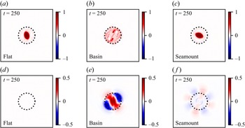


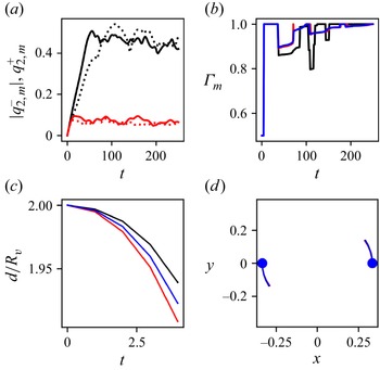


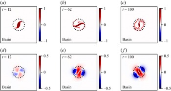


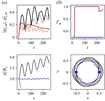


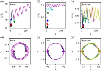


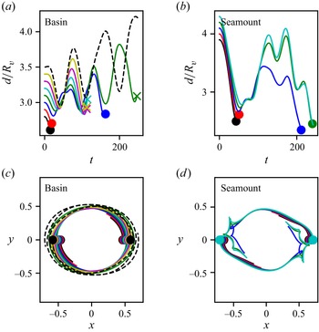


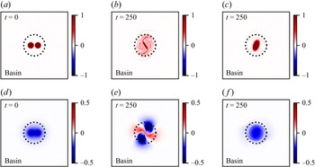


 Open access

