


1 Introduction
1.1 Applications of yield stress fluids
Gels are usually particulate dispersions that undergo solid–liquid or sol-gel transition i.e. they yield beyond a critical shear stress (called the yield stress  $\unicode[STIX]{x1D70F}_{y}$); they have many applications in industry (for e.g. in food products like mayonnaise, consumer products like toothpaste and drugs, building materials like concrete and paint, oil and drilling muds, etc. Bird, Dai & Yarusso (Reference Bird, Dai and Yarusso1983)), in biology (for e.g. blood flow Picart et al. (Reference Picart, Piau, Galliard and Carpentier1998)) and the environment (for e.g. clay suspension, debris, snow avalanches, lava flows, etc. Ancey (Reference Ancey2007) and Chambon, Ghemmour & Naaim (Reference Chambon, Ghemmour and Naaim2014)). Before yielding, they have solid-like properties e.g. they can sustain shear stress and deform elastically, whereas after yielding they behave like a fluid. Thus, the yield stress $\unicode[STIX]{x1D70F}_{y}$ is a practically useful parameter. To give some examples, it is used to assess the shelf life of paints, keep particulate fillers from settling in many consumer products and also dictates whether bubbles remain trapped in cement (Singh & Denn Reference Singh and Denn2008). The latter is an important factor in the structural integrity of buildings.
The yield stress  $\unicode[STIX]{x1D70F}_{y}$ has its origin in the microstructure of the material, which can dynamically adjust under the action of a flow. Hence, thixotropic (time-dependent shear thinning) behaviour is generally observed for many materials (e.g. clay suspension, colloidal gels) and $\unicode[STIX]{x1D70F}_{y}$ may not exhibit a single invariant value (Bonn & Denn Reference Bonn and Denn2009). Apart from this, yield stress fluids (YSF) may possess complex macroscopic properties because of their different elastic, viscous and plastic characteristics (Piau Reference Piau2007). For a recent comprehensive review describing the properties of YSF, please refer to Bonn et al. (Reference Bonn, Denn, Berthier, Divoux and Manneville2017).
1.2 Non-dimensional numbers
The Herschel–Bulkley (HB) constitutive equation (i.e. the relation between stress  $\unicode[STIX]{x1D70F}$ and strain rate $\dot{\unicode[STIX]{x1D6FE}}$) is the archetypical form used for YSF, and is given as $\dot{\unicode[STIX]{x1D6FE}}=0$ when $\unicode[STIX]{x1D70F}\leqslant \unicode[STIX]{x1D70F}_{y}$, and $\unicode[STIX]{x1D70F}=\unicode[STIX]{x1D70F}_{y}+\unicode[STIX]{x1D705}\dot{\unicode[STIX]{x1D6FE}}^{n}$ when $\unicode[STIX]{x1D70F}\geqslant \unicode[STIX]{x1D70F}_{y}$. Here, the power law exponent $n$ is the flow behaviour index i.e. it quantifies the degree of non-Newtonian behaviour, and $\unicode[STIX]{x1D705}$ is the consistency parameter. For the special case of $n=1$, known as the Bingham plastic model, $\unicode[STIX]{x1D705}$ is called the plastic viscosity.
The generalised Bingham number  $Bi$ or equivalently, Oldroyd $Od$ or Herschel–Bulkley number, is the ratio of plastic (yield stress) to viscous (shear stress) effects. The average wall-shear stress $\unicode[STIX]{x1D70F}_{w}$, which is proportional to the streamwise pressure gradient $\unicode[STIX]{x0394}P/\unicode[STIX]{x0394}x$, can be used to define $Bi=\unicode[STIX]{x1D70F}_{y}/((H/2)(\unicode[STIX]{x0394}p/\unicode[STIX]{x0394}x))$. Here, $H$ is the half-height in the case of a square duct or the radius in the case of a round pipe. Alternately, one can use the nominal shear stress based on the HB model to define $Bi=\unicode[STIX]{x1D70F}_{y}/(\unicode[STIX]{x1D705}(U/L)^{n})$, where $U$ and $L$ are the characteristic velocity and length scale respectively. The former definition is used in this work.
The choice of a representative Reynolds number  $Re^{\ast }$ for non-Newtonian fluids is often motivated by its ability to correctly predict the laminar friction factor $f=\unicode[STIX]{x1D70F}_{w}/(0.5\unicode[STIX]{x1D70C}U_{Bulk}^{2})$, according to a relationship $f=16/Re^{\ast }$ (see Metzner & Reed Reference Metzner and Reed1955), where $\unicode[STIX]{x1D70C}$ is the density and $U_{Bulk}$ is the average or bulk velocity of the fluid. Note that we have used the Fanning friction factor in this study. Using the Rabinowitsch–Mooney equation, Kozicki, Chou & Tiu (Reference Kozicki, Chou and Tiu1966) provided a general framework to predict the flow rate as a function of the streamwise pressure gradient for flow of non-Newtonian fluids in ducts of arbitrary cross-section, yielding a $Re^{\ast }$ consisting of two shape factors corresponding to the shape of the duct. Later, Liu & Masliyah (Reference Liu and Masliyah1998) improved the accuracy of the above relationship by proposing a three shape-factor approach that is better suited for ducts, where the wall-shear rate has contributions from terms other than only the wall-normal streamwise velocity gradient. The above approach has been used in the present study to define a generalised Reynolds number as
 $$\begin{eqnarray}Re^{\ast }=\frac{16}{f}=\frac{8\unicode[STIX]{x1D70C}U_{Bulk}^{2}}{\displaystyle \unicode[STIX]{x1D70F}_{y}+\unicode[STIX]{x1D705}\left(\frac{2U_{Bulk}a}{H}\right)^{n}\left(1+\frac{1-n}{bn}\right)^{n}c^{n-1}}.\end{eqnarray}$$
 The constants are  $a=1.778$, $b=4.382$ and $c=1.067$ for a square duct (Liu & Masliyah Reference Liu and Masliyah1998). It should be noted that (1.1) has strictly been evaluated for a generalised Newtonian fluid i.e. purely viscous (including viscoplastic), inelastic and time-independent fluid. However, the laminar friction factor $f$ for even strongly viscoelastic fluid flows has been shown to be the same as that for the generalised Newtonian fluids, provided that an appropriate Reynolds number such as $Re^{\ast }$ is used. This is true for laminar viscoelastic fluid flow in a circular pipe (see Cho & Harnett (Reference Cho and Harnett1982), where it is explicitly mentioned that there is no effect of elasticity). In the case of duct flows, viscoelasticity can generate secondary flows in the laminar regime, as will be discussed later. Even for such cases, it is shown that $16/Re^{\ast }$ is a very good estimate of the friction factor (see Hartnett & Kostic (Reference Hartnett and Kostic1985) and Hartnett, Kwack & Rao (Reference Hartnett, Kwack and Rao1986), for a rectangular duct and square duct respectively), thus affirming that the secondary flow has a very small effect on the pressure drop (also shown in Dodson, Townsend & Walters (Reference Dodson, Townsend and Walters1974)).
1.3 YSF in a square duct
Square duct flows of YSF, mostly of the Bingham type, have been a subject of several numerical studies. Following Taylor & Wilson (Reference Taylor and Wilson1997), Van Pham & Mitsoulis (Reference Van Pham and Mitsoulis1998) performed simulations of laminar duct flow using the Bingham model and proposed a master curve relating the flow rate to the pressure drop; useful information in the design of extrusion geometries. Saramito & Roquet (Reference Saramito and Roquet2001) used the augmented Lagrangian method for a Bingham model fluid flow in a square duct at varying  $Bi$ to compute the critical value of $Bi$ above which the flow stops, known as the stopping criterion (also see Mosolov & Miasnikov (Reference Mosolov and Miasnikov1965)). Huilgol & You (Reference Huilgol and You2005) extended the above method to a HB fluid model and found that, for a fixed $Bi$ (or $Od$ in their case), the plug region increases as the power law exponent in the HB model decreases.
A YSF may also display elastic properties both below and above yield stress, thus behaving like a viscoelastic solid before yielding and a viscoelastic liquid after yielding. Recently, Fraggedakis, Dimakopoulos & Tsamopoulos (Reference Fraggedakis, Dimakopoulos and Tsamopoulos2016b) compared the prediction from different elastoviscoplastic constitutive models in simple rheometric flows. Letelier, Siginer & González (Reference Letelier, Siginer and González2017) introduced elasticity in their simulations of a Bingham fluid for an approximate square duct geometry and observed that, for a fixed  $Bi$, the flow rate increases with increasing elasticity (quantified using a Weissenberg number $Wi$, which is the ratio of elastic stresses in the form of a normal-stress difference to the viscous stress due to shear forces). In a later work by the same authors, by including higher-order terms in $Wi$, a secondary flow in the form of streamwise vortices is seen (Letelier et al. Reference Letelier, Barrera, Siginer and González2018). Increasing the $Bi$ at the same $Wi$ reduced the intensity of the secondary flow, and displaced the vortices further away from the centre of the duct. Similar observations are also reported in this work, the novelty being the HB nature of the experimental fluid against the Bingham numerical model along with a higher $Bi$ in our case compared to their simulations, as will be described in the following sections. Often a Deborah number $De$ is defined as the ratio of the relaxation time of the fluid $\unicode[STIX]{x1D706}$ to the characteristic observation time scale of the flow $T_{f}$. Under certain circumstances, $De=\unicode[STIX]{x1D706}/T_{f}$ is equivalent to the $Wi$ (Poole Reference Poole2012b), which is more appropriately related to the characteristic rate of deformation (Dealy Reference Dealy2010). Since both $Wi$ and $Re^{\ast }$ increase with the flow rate for a given elastoviscoplastic fluid, an elasticity number $El$ is defined as $Wi/Re^{\ast }$ to quantify the effects of elastic forces compared to inertial forces.
Many researchers since Ericksen (Reference Ericksen1956) have investigated the existence and strength of the aforementioned streamwise vortices in laminar rectangular duct flows. This secondary flow originates from viscoelastic forces in non-circular pipes, specifically the second normal-stress difference (Dodson et al. Reference Dodson, Townsend and Walters1974), and its strength increases with the elasticity (Debbaut & Dooley Reference Debbaut and Dooley1999). Thus, no secondary flow would be observed in a purely viscous or viscoplastic fluid or for a certain special relationship between the second normal-stress difference and the fluid viscosity (Xue, Phan-Thien & Tanner Reference Xue, Phan-Thien and Tanner1995). Despite being very weak (around two orders in magnitude lower than the mean axial velocity), the presence of such a secondary velocity field may have substantial effects on the rate of heat transfer (Kostic Reference Kostic1994; Gao & Hartnett Reference Gao and Hartnett1996). Its weak nature also presents challenges in measuring it experimentally (Schroeder & Jeffrey Reference Schroeder and Jeffrey2011). Yue, Dooley & Feng (Reference Yue, Dooley and Feng2008) provided a general criterion to predict the direction of these secondary flows.
1.4 Studies in particle-laden flow
Dispersed phases like particles, drops or bubbles may appear as desired or undesired components in the final product made using YSF. Hence, their interaction with YSF is of practical importance and this paper partly addresses this problem.
In the case of particle-laden flows, sedimentation of a single spherical particle in a YSF is the most common study on account of its obvious importance in gaining fundamental understanding and as a precursor for multi-particle problems. A heavy isolated particle can settle inside a YSF only when the buoyancy force exceeds the resistance offered by the yield stress. Accordingly, a dimensionless yield–gravity parameter  $Y=\unicode[STIX]{x1D70F}_{y}/((\unicode[STIX]{x1D70C}_{p}-\unicode[STIX]{x1D70C}_{f})gd_{p})$ can be defined such that the particle moves only when $Y$ is lower than a threshold critical value ${\approx}0.2$ while noting that the exact value is still a topic of investigation (Chhabra Reference Chhabra2006). Creeping flow of an ideal yield stress fluid (Bingham or Herschel–Bulkley) around a sphere is reversible and displays fore–aft symmetry (Beaulne & Mitsoulis Reference Beaulne and Mitsoulis1997; Putz & Frigaard Reference Putz and Frigaard2010).
1.5 Need for careful preparation of the solution
In contrast to the above observation, when Putz et al. (Reference Putz, Burghelea, Frigaard and Martinez2008) performed particle image velocimetry (PIV) measurements of the flow field around a spherical particle sedimenting in a Carbopol solution at low  $Re<1$, they observed a breaking of the symmetry that is not observed in Newtonian fluids. In particular, the characteristics of the flow regions around the falling sphere were associated with the rheological properties of the fluid, thus calling for numerical models to include both elastic (Fraggedakis, Dimakopoulos & Tsamopoulos Reference Fraggedakis, Dimakopoulos and Tsamopoulos2016a) and hysteresis/thixotropic effects to accurately reproduce experimental observations as well as for experiments to ensure careful preparation of the fluid. On the other hand, Tabuteau, Coussot & de Bruyn (Reference Tabuteau, Coussot and de Bruyn2007) could obtain reproducible results in experiments for the drag on a settling sphere, in agreement with the simulations of Beaulne & Mitsoulis (Reference Beaulne and Mitsoulis1997). The authors attributed this to the careful preparation (homogenising for ten days!) of the yield stress fluid.
Indeed, in the recent work by Dinkgreve et al. (Reference Dinkgreve, Fazilati, Denn and Bonn2018), it was clearly shown that the discrepancy in the simple yield stress behaviour of Carbopol observed in previous studies was most likely due to lack of optimal mixing. At low shear rates, transient shear banding (Divoux et al. Reference Divoux, Tamarii, Barentin and Manneville2010) may occur that can cause apparent hysteresis in the flow curve i.e. the relation between shear stress and shear rate in simple shear, due to a lack of sufficient measurement time. The measurement time required to reach a steady state approaches unrealistically large values in the presence of wall slip, which occurs when a smooth rotating surface is used during rheometry (Poumaere et al. Reference Poumaere, Moyers-González, Castelain and Burghelea2014).
1.6 Particle migration in non-Newtonian fluids
Since the Carbopol gel used in this study exhibits small but measurable elastic effects both below and above the yield stress, the normal stresses and ensuing secondary flows are expected to affect the particle migration and their equilibrium distribution. Hence, a review of particle migration inside a duct flow of viscoelastic fluid is appropriate.
Cross-stream particle migration in viscoelastic fluids is quite different to their migration in a Newtonian fluid (D’Avino & Maffettone Reference D’Avino and Maffettone2015). In the absence of inertia, which is typical of microfluidic applications (e.g. cell focussing and separation), depending on the initial particle position, fluid elasticity drives the particle towards the channel centreline or the closest wall and from there towards the nearest corner in case of a duct geometry (Villone et al. Reference Villone, D’avino, Hulsen, Greco and Maffettone2013). This can be understood by observing the distribution of the first normal-stress difference, which has local minima at the centre and the corners of the duct cross-section (Yang et al. Reference Yang, Kim, Lee, Lee and Kim2011). The shear-thinning effects reduce the first normal-stress difference (Li, McKinley & Ardekani Reference Li, McKinley and Ardekani2015) thus, augmenting particle migration towards the closest wall (D’Avino et al. Reference D’Avino, Romeo, Villone, Greco, Netti and Maffettone2012). When second normal-stress differences are present (e.g. in a duct), the particle migration velocity, proportional to  $De(d_{p}/(2H))^{2}$, may be higher or lower than the ensuing secondary flow velocity, proportional to $De^{4}$ (Yue et al. Reference Yue, Dooley and Feng2008). Note that the observation time $T_{f}$ in the definition of $De$ above is taken as the inverse of the nominal shear rate: $T_{f}=1/(U_{Bulk}/H)$ by Villone et al. (Reference Villone, D’avino, Hulsen, Greco and Maffettone2013). Thus, at larger $De$ and smaller particle confinement $d_{p}/(2H)$, the secondary flow may overcome the migration velocity and the particle may also find a stable position near the centre of the streamwise vortices that are characteristic of the secondary flow (Villone et al. Reference Villone, D’avino, Hulsen, Greco and Maffettone2013).
It is shown by Seo, Kang & Lee (Reference Seo, Kang and Lee2014) that complex interplay between elasticity, inertia, shear thinning and confinement can lead to multiple stable and unstable equilibrium configurations. Lim et al. (Reference Lim, Ober, Edd, Desai, Neal, Bong, Doyle, McKinley and Toner2014a) realised that particles in microfluidic flows can be focussed at a high throughput rate even at very high  $Re\approx 10\,000$ i.e. high inertia, provided that the elastic normal stresses also increase proportionally i.e. the important criterion governing particle focussing is the elasticity number $El$.
$El$.
In the Stokes regime i.e. negligible particle inertia, flow of a particle suspension in a YSF inside a tube has been recently simulated by Siqueira & de Souza Mendes (Reference Siqueira and de Souza Mendes2019) using a regularised viscosity function, with the diffusive flux model (Phillips et al. Reference Phillips, Armstrong, Brown, Graham and Abbott1992) being used to describe the shear-induced particle migration. Particles were found to concentrate at the boundary of the plug and with increasing particle concentration, the maxima shifted towards the tube wall. No particles were found inside the plug due to the high but finite viscosity gradient (due to the regularisation) that slowly pushed them radially outwards. A similar method was used to model the particle migration for a tube flow of a Bingham fluid in Lavrenteva & Nir (Reference Lavrenteva and Nir2016). The maximum particle concentration was found at the interface between the yielded and unyielded regions. On the other hand, in the simulations of Hormozi & Frigaard (Reference Hormozi and Frigaard2017) to model particle-laden flow in a fracture, particles were found to concentrate in the plug.
1.7 Importance of the present study
Most of the above experimental studies concerning particle migration are microfluidic in their treatment i.e. they have a very low fluid and particle inertia. Also, they deal with a very low particle concentration  $(\unicode[STIX]{x1D6F7}\leqslant 0.1\,\%)$ i.e. negligible inter-particle interactions, that is typical of flow-focusing experiments, and to our knowledge there have not been many experimental studies devoted to multi-particle dynamics with the exception of the impressive observations made by Gauthier, Goldsmith & Mason (Reference Gauthier, Goldsmith and Mason1971) and Tehrani (Reference Tehrani1996) a while ago. A noteworthy contribution of this study lies in extending previous scientific investigations beyond the above regimes using a novel set-up with a large flow cross-section where the flow can be resolved at the particle scale, a feature that is very difficult to capture in microfluidic devices. In addition, the presence of yield stress in the suspending fluid and its interaction with the finite-size dispersed phase is expected to complement studies using the continuum-based approaches e.g. Hormozi & Frigaard (Reference Hormozi and Frigaard2017).
1.8 Outline
In the following sections, we start by describing the experimental set-up and the PIV–PTV (particle tracking velocimetry) measurement techniques. The fluid rheology and particle properties are also mentioned. Later, in the results section, we first describe the single-phase flow of two YSFs, with high (HYS) and low (LYS) yield stresses, at varying  $Re^{\ast }$ and $Bi$. This is then followed by the results concerning the particle-laden cases. Finally, in the discussion section, we try to interpret the above results by supporting our main observations with simple visual images obtained from shadowgraphy experiments, which are described therein. This is followed by a summary of the main conclusions.
2 Experimental technique
2.1 Experimental set-up
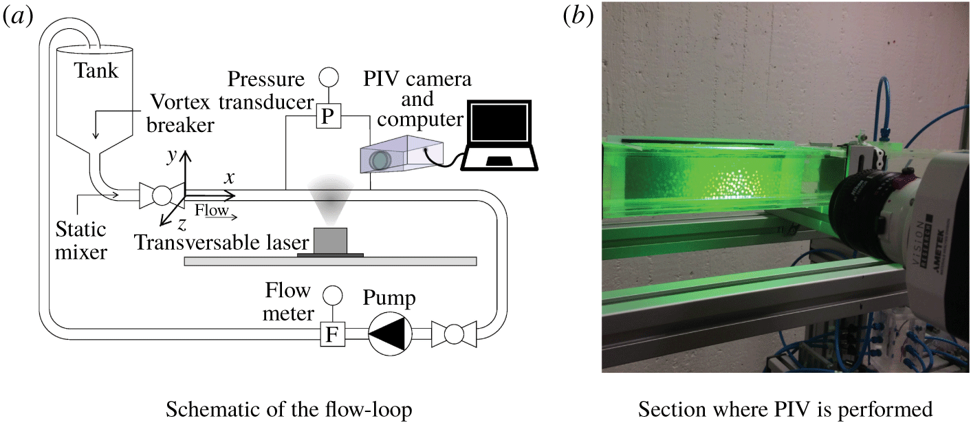
The experimental set-up used in this study has been previously used in Zade et al. (Reference Zade, Costa, Fornari, Lundell and Brandt2018) to investigate particle-laden turbulent flows of Newtonian and non-Newtonian flows up to  $\unicode[STIX]{x1D719}=20\,\%$, and is shown in figure 1. Only the most important features are described here and the interested reader is referred to the previous publications for additional details. The flow loop consists of a 5 m long transparent square duct with $50~\text{mm}\times 50~\text{mm}$ cross-section (refer to figure 1a). The particles are introduced in the conical tank and are circulated through the loop for a long enough time before measurements begin, so that they homogeneously disperse in the carrier fluid. A static mixer (Vortab Company, CA, USA) is installed close to the inlet of the duct to neutralise any swirling motions that may arise from the long $90^{\circ }$ bend at the exit of the tank. The temperature is maintained at nearly $20\,^{\circ }\text{C}$ by means of an immersed-coil heat exchanger in the tank. A very gentle disc pump (Model: 2015-8-2HHD Close coupled, Discflo Corporations, CA, USA) has been chosen, similar to Draad, Kuiken & Nieuwstadt (Reference Draad, Kuiken and Nieuwstadt1998), to minimise the mechanical breakage of the particles and avoid unwanted pulsations in the flow.
Experimental set-up. Reproduced from Zade et al. (Reference Zade, Costa, Fornari, Lundell and Brandt2018).
An electromagnetic flowmeter (Krohne Optiflux 1000 with IFC 300 signal converter, Krohne Messtechnik GmbH, Germany) is used to measure the volume flow rate of the particle–fluid mixture. The pressure loss is measured over a distance of  $54H$ starting at $140H$ from the inlet using a differential pressure transducer ( $0{-}1~\text{kPa}$, Model: FKC11, Fuji Electric France, S.A.S.). Data acquisition from the camera, flow meter and pressure transducer is performed using a National Instruments NI-6215 DAQ card using Labview™ software. The entry flow problem for YSF has been studied by Ookawara et al. (Reference Ookawara, Ogawa, Dombrowski, Amooie-Foumeny and Riza2000), amongst others, who proposed that the spatial development of the streamwise velocity at the edge of the plug is a suitable indicator for a fully developed flow. The development length was deduced in terms of a modified Reynolds number accounting for the plug radius, and for the maximum $Re^{\ast }$ encountered in our case, this development length would be less than $30H$. Thus, at our measurement location ${\approx}150H$, the flow can be considered to be fully developed for the single phase cases. For the particle-laden cases, the evolution of the particle concentration is qualitatively observed using shadowgraphy techniques, described later in the discussion section, and it is observed that an equilibrium concentration is established upstream of the measurement location.
2.2 Fluid rheology
An aqueous solution of Carbomer powder supplied as Carbopol® NF 980 (Lubrizol Corporation, USA), a commercial thickener, that is neutralised with sodium hydroxide (NaOH), is used as the model yield stress fluid. It is chosen due to its high transparency, small thixotropy and material stability (very slow ageing).
For each of our Carbopol batches, a weighed amount of Carbopol powder (0.25 % by weight) was first dispersed in 24 kg of water at room temperature  $({\sim}20\,^{\circ }\text{C})$. A high shear mixer (Silverson AX5, Silverson Machines, Inc., USA) was used to disperse the powder at a maximum of ${\sim}1200~\text{rpm}$ for up to ${\sim}30~\text{minutes}$. The dispersion was then left stationary for ${\sim}30~\text{minutes}$ to allow for air bubbles to evacuate. Then, a 18 wt./v % of NaOH solution at 2.3 times the mass of Carbomer powder was used to neutralise the dispersion. The NaOH was gradually added with a pipette whilst stirring the solution gently at low rotational speeds $({\sim}135~\text{rpm})$ using a helical mixer (RW 20 DZM-P4, IKA-Labortechnik, IKA-Werke GmbH & Co. KG, Germany). At the end of the neutralisation process, the pH was noted to be ideally within the required range (6.5–7.0) so as to ensure maximum swelling and, hence, a high yield stress. The neutralised solution was further mixed in a large cement mixer (1402 HR, AL-KO, Germany) at a low rotational speed for an ${\sim}5$ additional hours to ensure complete homogenisation.
The whole preparation process led to a concentrated solution with a high yield stress. Experiments had to be performed with a thinner (less viscous) fluid in order to facilitate pumping. Thus, the concentrated solution was gradually diluted in the flow loop by mixing with water and recirculating for  ${\sim}2~\text{hours}$ before measurements began. Since the shear rates in the flow loop are not extremely high, solution degradation and the resulting change in properties can be considered insignificant. Repeatability of the properties of the final solution was ascertained by (i) measuring the flow curves in a rheometer and (ii) by monitoring the pressure drop at a fixed flow rate. It was found that by systematically following the above mixing protocol, solutions with nearly the same pressure drop exhibiting the same flow curve were obtained repeatedly. In order to minimise the occurrence of bubbles arising due to dissolved gases in the water, tap water was heated so as to remove these dissolved gases and then cooled before being used for preparation of the Carbopol solution. Air bubbles entrained during introduction of the hydrogel particles were removed in the conical tank that is open to the atmosphere.
Flow curves (symbols) and the HB model fit (solid lines) for the LYS and HYS yield stress fluids. The open and closed symbols denote measurements during ascending and descending shear rates respectively.
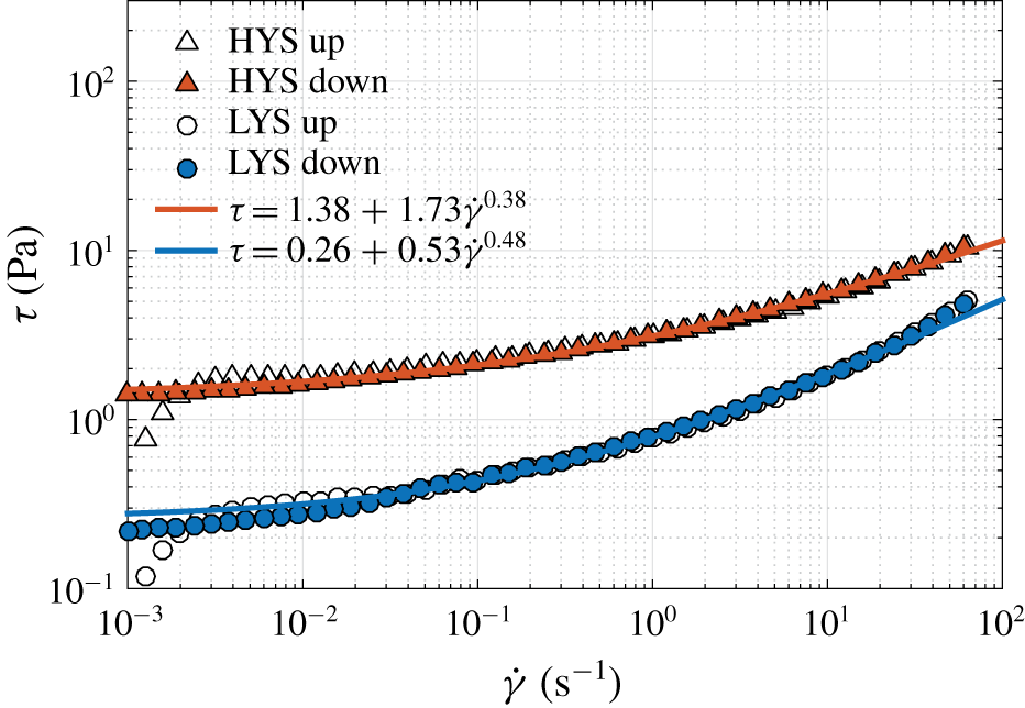
The rheological tests focused on the determination of the steady-state flow curve. They were performed using a TA AR-2000ex rheometer (TA Instruments, Inc., USA) with a vane and cup geometry. A pre-shear of  $300~\text{s}^{-1}$ was applied for 10 s followed by a rest period of 40 s to establish a reproducible state. Flow sweeps in both ascending and descending controlled shear rate were then carried out in a range of shear rates (0.001 to $80~1~\text{s}^{-1}$ with 10 points per decade) at room temperature to determine the flow curves and to check for thixotropy. This range of shear rates includes the maximum shear rate in the experiments. For each measurement point, the shear rate was held constant for 30 s. Figure 2 shows the flow curve for the two fluids used in this study. Elastic effects on start-up (Dinkgreve, Denn & Bonn Reference Dinkgreve, Denn and Bonn2017) were visible for a few points at low shear rates during the up sweep i.e. the accumulated strain was perhaps insufficient for the material to flow. Hence, the down sweep curve is used to fit the Herschel–Bulkley model, whose parameters are mentioned in the legend of figure 2. The repeatability of the flow curves was ensured by performing the above tests on three separate solutions prepared independently of each other, both before and after adding the particles, and an average curve is used. The working fluids display a shear-thinning behaviour after yielding i.e. they are yield pseudo-plastic fluids. The dynamic yield stress determined above (static yield stress is determined using creep tests) is low compared to other wall-bounded flow studies of YSF (see Güzel et al. (Reference Güzel, Burghelea, Frigaard and Martinez2009) and Escudier & Presti (Reference Escudier and Presti1996) amongst others) but for such flows, the non-dimensional $Bi$ is the relevant criterion to assess the importance of plasticity on the flow. This point about the relevance of $Bi$ will be illustrated further by means of velocity profiles that exhibit a solid plug.
Oscillatory measurements: amplitude of the strain,  $\unicode[STIX]{x1D6FE}$, sweeps at a fixed angular frequency $\unicode[STIX]{x1D714}=1~\text{Hz}$ for the two fluids used in this work.
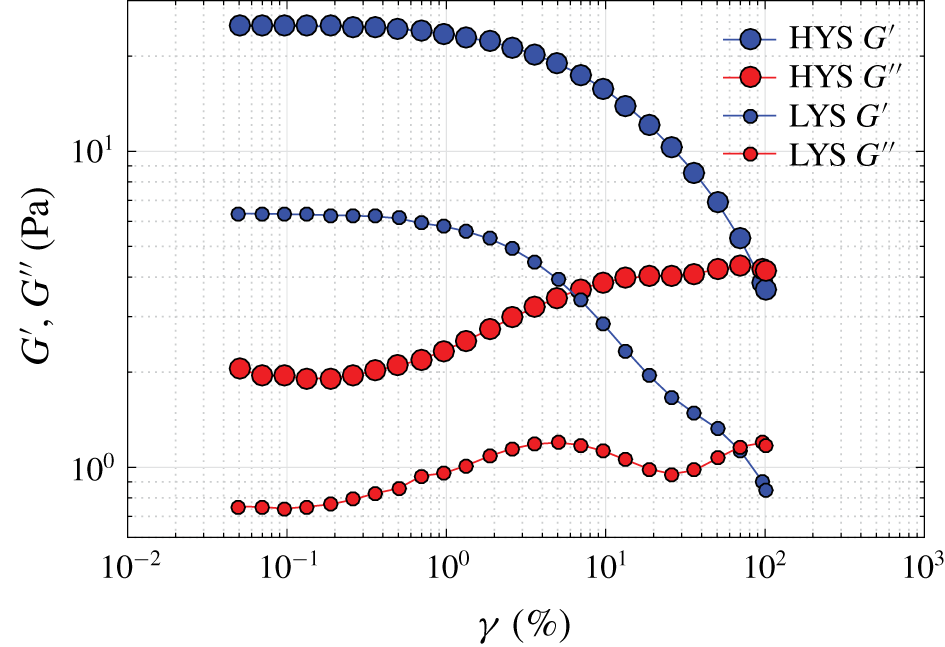
The viscoelastic behaviour near the yield limit is measured by oscillatory tests using a splined bob and cub attachment in a Kinexus pro+ rheometer (Malvern Panalytical, UK). The linear viscoelastic region that exists at small strain  $\unicode[STIX]{x1D6FE}$ amplitudes can be identified by nearly constant elastic $G^{\prime }$ and viscous $G^{\prime \prime }$ moduli over a wide range of strain amplitudes. This is shown in figure 3 where oscillatory measurements are performed at a frequency $\unicode[STIX]{x1D714}$ of 1 Hz. The point of cross-over between $G^{\prime }$ and $G^{\prime \prime }$ for each of the two fluids at 1 Hz, $H\unicode[STIX]{x1D70F}_{y}\sim 4~\text{Pa}$ and $L\unicode[STIX]{x1D70F}_{y}\sim 1~\text{Pa}$, is of a similar order of magnitude as the yield stress, albeit slightly larger. Figure 4 shows the variation of
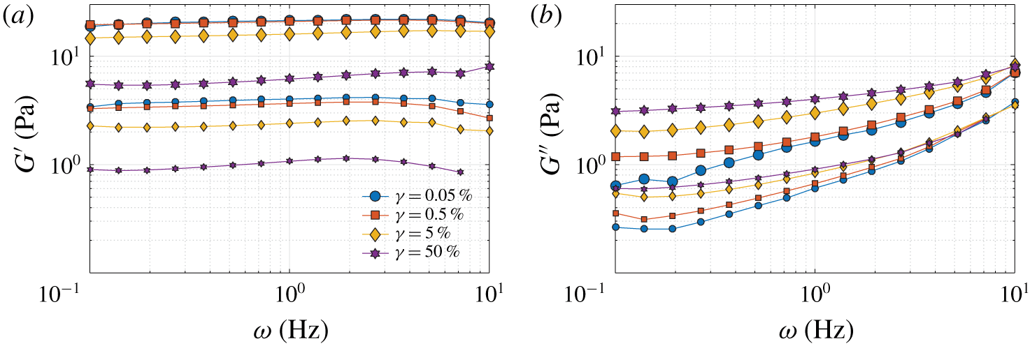
  $G^{\prime }$ and $G^{\prime \prime }$ with the frequency $\unicode[STIX]{x1D714}$ at multiple strain amplitudes $\unicode[STIX]{x1D6FE}$, starting from the linear and extending towards the nonlinear viscoelastic regime associated with yielding. In the linear regime i.e. at lower $\unicode[STIX]{x1D6FE}$, the elastic modulus $G^{\prime }$ (refer to figure 4a) is approximately flat and around one order of magnitude greater than the viscous modulus $G^{\prime \prime }$ (refer to figure 4b); $G^{\prime }$ and $G^{\prime \prime }$ are nearly independent of $\unicode[STIX]{x1D6FE}$ in this linear regime $(\unicode[STIX]{x1D6FE}\leqslant 0.5\,\%)$, as expected. As mentioned in Varges et al. (Reference Varges, Costa, Fonseca, Naccache and de Souza Mendes2019), at these low amplitudes the microgels deform elastically but they do not move significantly relative to each other and hence have a low internal dissipation (also see Piau Reference Piau2007). As the deformation amplitude increases, the microstructure starts breaking, causing elastohydrodynamic friction forces to rise and dissipation to increase, leading to a higher loss modulus. Finally, at higher $\unicode[STIX]{x1D6FE}$, outside the purview of small amplitude oscillatory shear, the elastic components decrease and the viscous components increase. Similar observations have been reported in Piau (Reference Piau2007), Gutowski et al. (Reference Gutowski, Lee, de Bruyn and Frisken2012), Firouznia et al. (Reference Firouznia, Metzger, Ovarlez and Hormozi2018) and Varges et al. (Reference Varges, Costa, Fonseca, Naccache and de Souza Mendes2019) amongst others. The viscoelastic moduli $G^{\prime }$ and $G^{\prime \prime }$ are relevant at small shear rates. In order to quantify the viscoelastic effects at higher shear rates, other steady-state viscometric functions namely, the first and second normal-stress differences: $N_{1}$ and $N_{2}$ needs to be measured. These measurements are fraught with difficulties in YSF and for $N_{1}$, both positive (Tehrani Reference Tehrani1996; Peixinho et al. Reference Peixinho, Nouar, Desaubry and Théron2005; Piau Reference Piau2007) and negative values (Janmey et al. Reference Janmey, McCormick, Rammensee, Leight, Georges and MacKintosh2007) are reported. In the recent work of De Cagny et al. (Reference De Cagny, Fazilati, Habibi, Denn and Bonn2019), the authors investigated common simple i.e. non-thixotropic YSF, including Carbopol, and found that $N_{1}>0$ and $N_{2}<0$ with $N_{1}>N_{2}$; they increase quadratically with the shear stress, both below and above the yield stress. The above authors proposed that, in the absence of normal-stress measurements, $N_{1}$ can be estimated by using the linear elastic modulus $G^{\prime }$ as $N_{1}\sim \unicode[STIX]{x1D70F}^{2}/G^{\prime }$. Here, $\unicode[STIX]{x1D70F}$ is the shear stress and, for our fluids, this implies that $N_{1}<6~\text{Pa}$ (for LYS at the maximum shear rate of figure 2). Such small values are quite difficult to measure, especially due to normal force drift and inertia (Poole Reference Poole2012a). It was hence not possible to accurately measure the normal-stress differences for our weakly elastic fluid. Nevertheless, viscoelasticity of Carbopol after yielding has been observed in many studies (e.g. see Taylor & Bagley Reference Taylor and Bagley1974; Laurencena & Williams Reference Laurencena and Williams1974). Peixinho et al. (Reference Peixinho, Nouar, Desaubry and Théron2005) also observed substantial drag reduction in turbulent flow of Carbopol, a typical viscoelastic effect.
Oscillatory measurements: frequency  $\unicode[STIX]{x1D714}$ sweeps to determine (a) the elastic modulus $G^{\prime }$ and (b) the viscous modulus $G^{\prime \prime }$ for several strain amplitudes. The larger and smaller symbols refer to the HYS and LYS cases, respectively.
2.3 Particle properties
As already noted in our previous work (Zade et al. Reference Zade, Costa, Fornari, Lundell and Brandt2018) the particles are commercially procured super-absorbent (polyacrylamide-based) hydrogel spheres which are delivered in dry form. After grading them into different sizes using sieves, one fairly mono-dispersed fraction is used in these experiments. These dry particles are mixed with tap water that has a very small amount of fluorescent rhodamine dye (a few ppm) dissolved in it, and then left submerged for around one day. Ultimately, they grow to an equilibrium size of  $4.2\pm 0.8~\text{mm}$ (3 times standard deviation), thus yielding a duct height to particle diameter ratio $2H/d_{p}$ of ${\sim}12$. The tiny amount of rhodamine is absorbed by each particle, and makes them glow in the laser sheet, so that they can be detected in the PIV images, as will be shown later. The particle size was determined both by a digital imaging system and from the PIV images of particles in the flow. A small Gaussian-like spread in the particle diameter was observed. The fact that a Gaussian-like particle size distribution has a small effect on the flow statistics has already been shown in Fornari, Picano & Brandt (Reference Fornari, Picano and Brandt2018).
The density ratio of the particle to tap water  $\unicode[STIX]{x1D70C}_{p}/\unicode[STIX]{x1D70C}_{f}$ is found to be equal to $1.0035\pm 0.0003$. Since the final concentration of Carbomer in the working fluid is less than 0.1 %, the change in density of the fluid from tap water is assumed to be insignificant. Since the typical flow velocities are relatively small $(U_{Bulk}<0.3~\text{m}~\text{s}^{-1})$ in the present flow configuration, the corresponding dynamical forces are low under these conditions and the hydrogel particles did not exhibit any visible deformation (as also confirmed from the time-resolved movies of the particles in flow). Also, as pointed out by Gondret, Lance & Petit (Reference Gondret, Lance and Petit2002), for the low impact Stokes number, collisions between particles or between a particle and the wall are dominated by viscous effects, and particles do not rebound i.e. the effective coefficient of restitution will be very small. Based on the above arguments, the particles can be considered to behave as rigid spheres. For details about the density measurements and calculations pertaining to the restitution coefficient, the reader is referred to our previous work (Zade et al. Reference Zade, Fornari, Lundell and Brandt2019a).
2.4 Velocity measurement technique
The coordinate system is sketched in figure 1(a) with  $x$ in the streamwise, $y$ in the wall-normal and $z$ in the spanwise directions. The velocity field is measured using two-dimensional PIV (2D-PIV) in multiple spanwise planes ( $z/H=0$ to 1) to measure the inhomogeneous velocity field in the square duct. The PIV set-up consists of a continuous wave laser $(\text{wavelength}=532~\text{nm},\text{power}=2~\text{W})$ and a high-speed camera (Phantom Miro 120, Vision Research, NJ, USA), as shown in figure 1(b). The thickness of the laser light sheet is 1 mm. The seeding particles are hollow glass microspheres (Sphericel® 110P8, Potters industries Inc., $d_{p}=9{-}13~\unicode[STIX]{x03BC}\text{m}$, $\unicode[STIX]{x1D70C}_{p}=1.10\pm 0.05~\text{gm}~\text{cm}^{3}$) and polyamide microspheres ( $d_{p}\approx ~55~\unicode[STIX]{x03BC}\text{m}$, $\unicode[STIX]{x1D70C}_{p}=1.2~\text{gm}~\text{cm}^{-3}$). The following paragraphs are briefer reproductions of the PIV–PTV algorithm already described in Zade et al. (Reference Zade, Fornari, Lundell and Brandt2019a).
PIV image pairs are captured at a resolution of approximately  $60~\text{mm}/1024~\text{pixels}$; the size of the measurement section is $50~\text{mm}\times 50~\text{mm}$. For each flow rate, a time delay was chosen so that the maximum pixel displacement, based on the mean velocity, did not exceed a quarter of the size of the final interrogation window (IW) (Raffel et al. Reference Raffel, Willert, Wereley and Kompenhans2013). Thus, it can range from $36\times 10^{-3}~\text{s}$ for the $\text{lowest flow rate}=2~\text{l}~\text{min}^{-1}$ (litres per minute), to approximately $1.8\times 10^{-3}~\text{s}$ for the $\text{highest flow rate}=40~\text{l}~\text{min}^{-1}$. The exposure time is kept small enough $({<}0.1\times 10^{-3}~\text{s})$ so that enough light is captured by the camera sensor while pixel displacement within one frame is significantly less than 1 pixel. Images were processed using an in-house, three-step, fast Fourier transform (FFT)-based, cross-correlation algorithm (Kawata & Obi Reference Kawata and Obi2014). The degree of overlap is approximately 47 % and can be estimated from the fact that the corresponding final resolution is $1~\text{mm}\times 1~\text{mm}$ per IW. Between 200 and 400 image pairs have been observed to be sufficient to ensure statistically converged results.
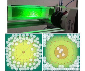
Images involved to calculate the fluid and particle velocity fields. The raw image (a) is used for PIV analysis. The enhanced image (b) is used to detect circles and for the subsequent PTV analysis. The combined PIV (for fluid phase denoted by green arrows) and PTV (for particle phase denoted by blue arrows) velocity field is shown in (c). The detected particles are also shown in (b). The above images correspond to LYS fluid,  $\unicode[STIX]{x1D719}=10\,\%$, $z/H=0.9$ and $Re^{\ast }=156$.
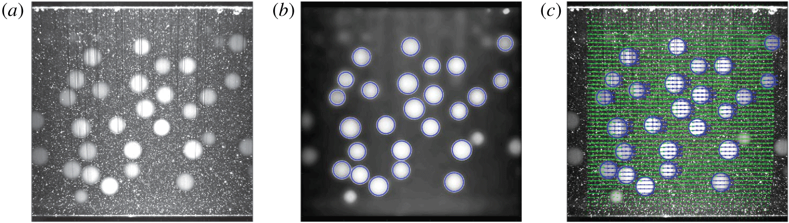
Figure 5(a) depicts one image from a typical PIV sequence for particle-laden flow. Raw images captured during the experiment were saved in groups of two different intensity levels. The first group of images, a typical example being figure 5(a), were used for regular PIV processing according to the algorithm mentioned above to find the fluid velocity field. The same first group of images were later contrast enhanced in the post-processing step and constituted the second group of images, an example being figure 5(b). These second group of images were used to detect the particles. Again, the details of the image post-processing and the PTV algorithm are explained at length in Zade et al. (Reference Zade, Fornari, Lundell and Brandt2019a).
The velocity of both the fluid and particle phases is defined on a spatially fixed Eulerian grid. Consequently, a mask matrix is defined, which assumes the value 1 if the point lies inside the particle and 0 if it lies outside the particle. The particle velocity is determined using PTV at its centre, which is assigned to the grid points inside the particle  $(\text{mask}=1)$. The velocity field of the particle phase is now available at the same grid points as that of the fluid and the ensemble averaging, reported later, are phase averaged statistics. Figure 5(c) shows the combined fluid (PIV) and particle (PTV) velocity field. It may be observed that the intensity of the laser sheet is weaker away from the centre of the images and particles are not accurately detected in this region. Hence, PIV and PTV results are extracted from a reduced area neglecting this poorly illuminated region, as shown in figure 5(c).
3 Results
The results are described first in terms of the pressure drop. The velocity field for single-phase flow is described later, before the velocity and concentration profiles for the particle-laden cases are presented.
3.1 Pressure drop
Figure 6(a) displays the friction factor  $f$ as a function of the Reynolds number $Re^{\ast }$ for all the cases investigated in this study. The single-phase cases seem to agree reasonably well with the $16/Re^{\ast }$ curve, which is the analytical solution for Poiseuille flow of a Newtonian fluid. This is noteworthy considering the fact that a complex expression is used to define $Re^{\ast }$, see (1.1). There are measurable changes due to the addition of particles and to better appreciate them, the data in the figure are re-plotted as a percentage change compared to the analytical solution $16/Re^{\ast }$ in figure 6(b). The deviation for single-phase flow is higher at the lowest $Re^{\ast }$ for HYS fluid but drops to values very close to the analytical solution for higher $Re^{\ast }$. At particle volume fraction $\unicode[STIX]{x1D719}=5\,\%$, within the extent of the error bars, the increase in pressure drop is independent of the suspending fluid and $Re^{\ast }$. The departure in pressure drop from the single-phase case is more pronounced for $\unicode[STIX]{x1D719}=10\,\%$. Note that for $\unicode[STIX]{x1D719}=10\,\%$, experiments are conducted only in LYS.
(a) Variation of friction factor  $f$ with $Re^{\ast }$ for both single-phase and particle-laden cases. (b) The percentage deviation of the measured $f$ compared to the $f$ expected for single-phase laminar flow. The inset in (b) shows the same plot but with a Reynolds number ${Re_{e}}^{\ast }$ accounting for the additional suspension viscosity due to particles: the filled symbols are based on the Eilers fit and the unfilled symbols are based on a suspension having a modified yield stress and consistency (Chateau, Ovarlez & Trung Reference Chateau, Ovarlez and Trung2008).

The increase in the viscosity of a suspension due to the addition of hard spheres can be semi-empirically described using the Eilers fit (von Eilers Reference von Eilers1941) for a Newtonian suspending fluid under negligible inertia at the particle scale as  $\unicode[STIX]{x1D707}_{e}/\unicode[STIX]{x1D707}=(1+(5/4)\unicode[STIX]{x1D719}/(1-\unicode[STIX]{x1D719}/\unicode[STIX]{x1D719}_{Max}))^{2}$. This effective suspension viscosity $\unicode[STIX]{x1D707}_{e}$ is only a function of the nominal particle concentration $\unicode[STIX]{x1D719}$ and the maximum packing fraction $\unicode[STIX]{x1D719}_{Max}$, assumed here to be equal to the value for random-close packing ${\approx}65\,\%$. Note that for $\unicode[STIX]{x1D719}\leqslant 10\,\%$, changing $\unicode[STIX]{x1D719}_{Max}$ even by $\pm 10\,\%$ does not produce any substantial change in the estimate of $\unicode[STIX]{x1D707}_{e}$. In the limit of low particle inertia and a uniform particle distribution, it may be used to predict the change in the friction factor for a Newtonian suspending fluid. Accordingly, in the inset of figure 6(b), a new effective Reynolds number ${Re_{e}}^{\ast }$ is defined using $\unicode[STIX]{x1D707}_{e}$ such that ${Re_{e}}^{\ast }=Re^{\ast }\unicode[STIX]{x1D707}/\unicode[STIX]{x1D707}_{e}$ and the experimentally measured friction factor $f$ at $Re^{\ast }$ is compared to the expected friction factor $16/{Re_{e}}^{\ast }$ for an effective fluid (see filled symbols). A good collapse of all the data points within $\pm 5\,\%$ of the single-phase results is observed using this approach. A more appropriate rheological description of suspensions in YSF is provided by Chateau et al. (Reference Chateau, Ovarlez and Trung2008) and Mahaut et al. (Reference Mahaut, Chateau, Coussot and Ovarlez2008). Their experiments and theoretical arguments suggest that a particle suspension in YSF behaves like a Herschel–Bulkley fluid with the same flow index $n$ as the suspending YSF, but with a different equivalent yield stress $\unicode[STIX]{x1D70F}_{y}\sqrt{(1-\unicode[STIX]{x1D719})g(\unicode[STIX]{x1D719})}$ and consistency $\unicode[STIX]{x1D705}\sqrt{(g(\unicode[STIX]{x1D719}))^{n+1}/(1-\unicode[STIX]{x1D719})^{n-1}}$. The function $g(\unicode[STIX]{x1D719})$ is the Krieger–Dougherty fit for suspension viscosity: $g(\unicode[STIX]{x1D719})=(1-\unicode[STIX]{x1D719}/\unicode[STIX]{x1D719}_{Max})^{-2.5\unicode[STIX]{x1D719}_{Max}}$ (Krieger & Dougherty Reference Krieger and Dougherty1959) and is virtually indistinguishable from the Eilers fit (mentioned above) up to the low $\unicode[STIX]{x1D719}=10\,\%$ investigated in the present case. Using the above modification in yield stress and consistency, an equivalent Reynolds number, based on (1.1), can be defined and the corresponding laminar friction factor is (also) plotted in the inset of figure 6(b) (see unfilled symbols). Indeed, there are differences between the predictions using a simple effective viscosity (filled symbols) and the more reasonable modification in viscosity for YSF (unfilled symbols) proposed by Chateau et al. (Reference Chateau, Ovarlez and Trung2008). Both the above fits are based on the assumption of a homogeneous particle distribution and, as will be shown later, this is definitely not the case in our present experiments, where particles migrate to specific regions of the flow domain. Thus, there is no strong reason for an effective viscosity formulation to accurately predict the friction factor in laminar flows for a square duct. A more thorough investigation at multiple $\unicode[STIX]{x1D719}$, particle sizes, $Re^{\ast }$ and flow geometries is therefore required to test the effectiveness of the above approach. In our previous work (Zade et al. Reference Zade, Costa, Fornari, Lundell and Brandt2018), we have observed that the friction factor in a turbulent flow of Newtonian fluid is a function of both the particle volume fraction and size. Also, from the results in Zade, Lundell & Brandt (Reference Zade, Lundell and Brandt2019b), we learnt that the predictions from the Eilers fit diverge at higher volume fractions $\unicode[STIX]{x1D719}\geqslant 15\,\%$ for Newtonian turbulent flows.
(a) Streamwise and (b) wall-normal velocity profiles in different spanwise planes for high YSF (HYS). Flow rate  $(Q)=8~\text{l}~\text{min}^{-1}$, $Re^{\ast }=4$, $Bi=0.26$.
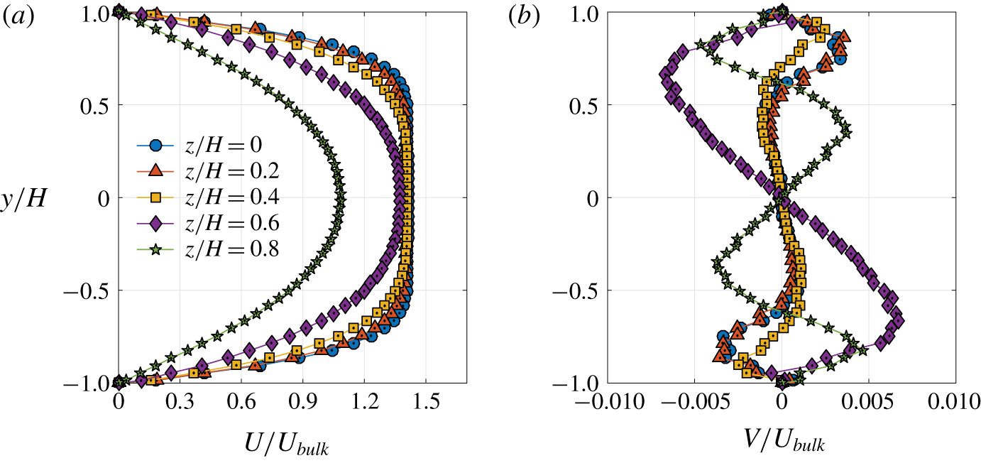
A mean secondary flow is also observed in the duct, as will be shown in the coming sections. However, considering the weak amplitude of this flow, it is assumed to have a negligible effect on the friction factor, as also previously observed by Gao & Hartnett (Reference Gao and Hartnett1993). Another point to note is that the Reynolds number, if defined using the viscosity at the wall as  $Re_{\unicode[STIX]{x1D707}_{Wall}}=\unicode[STIX]{x1D70C}U_{Bulk}(2H)/\unicode[STIX]{x1D707}_{Wall}$, is very similar in magnitude (within 10 %) to the $Re^{\ast }$ used in this study. The viscosity at the wall $\unicode[STIX]{x1D707}_{Wall}$, also used in the previous paragraph to estimate the particle scale Reynolds number, can be calculated using the flow curves in figure 2 and the average shear stress at the wall, estimated from the streamwise pressure gradient.
3.2 Velocity statistics for single-phase flow
For the single-phase flow, PIV measurements were performed in multiple spanwise planes. Mean profiles have been obtained by averaging in time and along the streamwise direction. An example of the results of such measurements is shown in figures 7 and 8 for HYS and LYS, respectively, for the same flow rate. The streamwise velocity profiles, normalised by the bulk velocity, display a flat region of constant velocity in the centre plane  $z/H=0$. This region of zero velocity gradient is representative of the solid plug and it shrinks while moving to a plane closer to the side wall $z/H=1$. At the same flow rate, the plug is larger for the thicker fluid HYS due to the high yield stress (compare figures 7a and 8a).
Caption similar to figure 7 but this time for the low YSF (LYS) at the same flow rate  $Q=8~\text{l}~\text{min}^{-1}$. $Re^{\ast }=12.5$, $Bi=0.15$.

Figures 7(b) and 8(b) show the variation of the wall-normal velocity profiles for the two fluids. Similar symbols represent similar planes. These velocities are a direct measure of the secondary flow and their maximum strength is close to 1 % of the bulk velocity. In the centre plane  $z/H=0$, the region of zero velocity gradient for the streamwise velocity has also a nearly zero wall-normal velocity i.e. there is no secondary flow inside the plug. The most striking feature comparing the two figures is that the intensity of the wall-normal velocities increases for the thinner fluid LYS. The plug region is smaller for LYS as deduced from the corresponding streamwise velocity profiles, allowing for a larger yielded region and hence, larger and stronger secondary flows. The action of the plug in damping the secondary flow was also observed in the simulations by Letelier et al. (Reference Letelier, Barrera, Siginer and González2018).
A rectangular duct flow is symmetric about the orthogonal axes  $z-z$ and $y-y$. In the special case of the square duct, the flow is also symmetric about its diagonals. Thus, measurements of two velocity components in a limited number of spanwise planes (as in the 2D-PIV used here) can be used to calculate all the three velocity components at other locations in the duct. This approach is illustrated in the schematic of figure 9. Thus, 2D-PIV measurements in $N$ planes (in figure 9, $N=5$ denoted by darker lines) can yield the three-dimensional velocity at $(2N-1)^{2}$ locations.
Schematic of the symmetry lines in a square duct (dash-dotted lines). The spanwise planes where PIV is performed are represented with a darker colour. The mirror images of these planes about the symmetry lines are represented by lighter version of the same colours. The intersection points of these planes correspond to locations where all three velocity components can be evaluated.
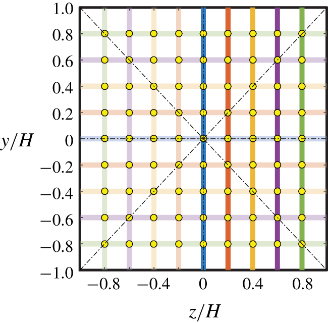
Variation of mean flow with increasing  $Re^{\ast }$ for the high YSF (HYS). The colour map corresponds to the mean streamwise velocity normalised by the bulk velocity. The arrows represent the direction and strength of the secondary flow. The plug region at the centre is delimited by the solid line.

The above technique is applied using  $N=9$ planes for three different flow rates or $Re^{\ast }$ of the thicker fluid HYS as shown in figure 10. The secondary flow can now be clearly visualised: it carries the high momentum fluid from the yielded regions around the core to the centre of the wall and low momentum fluid from the corners towards the core. The intensity of this secondary flow increases with increasing $Re^{\ast }$, coupled with the reduction of the plug size.
The extent of the plug at the duct core is determined as follows: a two-dimensional polynomial of sixth order is fitted to the streamwise velocity data (coefficient of determination  $R^{2}\geqslant 0.99$). A no-slip condition is assumed at the boundaries. Higher-order polynomials did not show any significant improvement in the quality of the fit. Using this fit, the streamwise velocity field was smoothly mapped on a plane of higher resolution ( $400\times 400$ points). The norm of the velocity gradient $\sqrt{(\unicode[STIX]{x2202}U/\unicode[STIX]{x2202}y)^{2}+(\unicode[STIX]{x2202}U/\unicode[STIX]{x2202}z)^{2}}$, using a simple forward difference scheme, is evaluated at each of these points and the plug is designated at those points where the norm is less than 1 % of its maximum value (occurs at the wall centre). This procedure naturally suggests the existence of small unyielded plug-like regions also at the corners where the velocity gradients are small. Despite the likely presence of these stagnant zones, as found in many previous numerical studies (Saramito & Roquet Reference Saramito and Roquet2001), they are not shown here due to their proximity to the corners where PIV measurements are not performed. Nevertheless, their size is assumed to be very small for the $Bi$ used in this study. The shape of the moving plug in the core region appears to be near circular, more so for higher $Re^{\ast }$ or, equivalently, lower $Bi$.
$Bi$.
(a) Change of Bingham number  $Bi$ as a function of the Reynolds number $Re^{\ast }$ for both the HYS and LYS yield stress fluids (single phase with no particles). Variation of maximum to bulk streamwise velocity ratio as a function of (b) Reynolds number $Re^{\ast }$ and (c) Bingham number $Bi$. The maximum velocity is measured using PIV and the bulk velocity is measured from the flow meter.
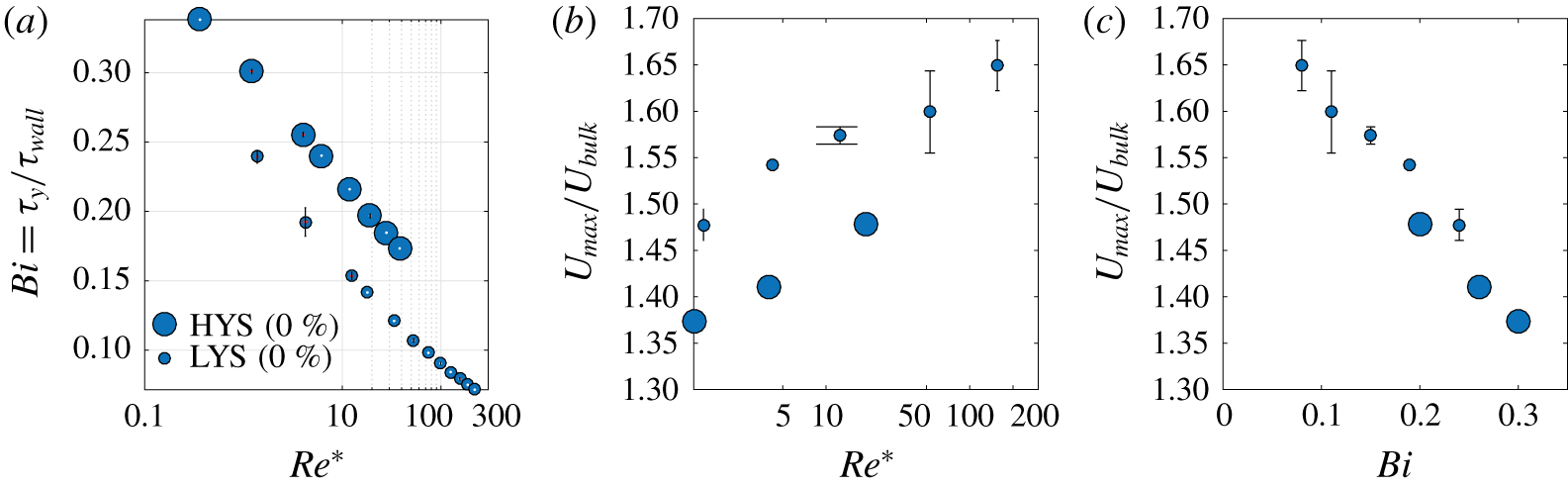
Figure 11(a) shows the variation of  $Bi$ with $Re^{\ast }$. For the same $Re^{\ast }$, the thicker fluid HYS has a larger $Bi$. As mentioned previously in the Introduction, if a Bingham number $Bi$ based on the HB parameters is defined as $Bi_{HB}=\unicode[STIX]{x1D70F}_{y}/(\unicode[STIX]{x1D705}(U/L)^{n})$, it ranges from 0.36 to 0.72 for HYS and from 0.14 to 0.43 for LYS i.e. around twice the value of the $Bi$ shown in figure 11(a). From Saramito & Roquet (Reference Saramito and Roquet2001), it can be expected that, with increasing $Bi$, both the moving plug at the centre and the stagnant plug at the corners grow. The growing plug in the core would become non-circular before finally merging with the plugs at the corner at some critical $Bi$, whose value for a strictly Bingham fluid was found to be $4/(2+\sqrt{(\unicode[STIX]{x03C0})})\approx 1.06$ (Mosolov & Miasnikov Reference Mosolov and Miasnikov1965). At this stage, the flow stops.
Figures 11(b) and 11(c) show the change in the ratio of the maximum to bulk velocity for different  $Re^{\ast }$ and $Bi$ respectively. By virtue of a higher yield stress, at the same $Re^{\ast }$, HYS has a larger plug than LYS and, hence, a flatter velocity profile i.e. a smaller $U_{Max}/U_{Bulk}$ (see figure 11b). Figure 11(c) shows that, at the same $Bi$, HYS has a smaller $U_{Max}/U_{Bulk}$ i.e. a larger plug region. This is in agreement with Huilgol & You (Reference Huilgol and You2005), who observed that the plug region is larger for a fluid with a lower power law exponent $n$, for fixed Bingham number $Bi$. From figure 2, it is deduced that LYS has a higher $n$ than HYS but a smaller plug, as indicated by the higher $U_{Max}/U_{Bulk}$.
Comparison of mean streamwise velocity in the plane of the wall bisector for different  $Bi=\unicode[STIX]{x1D70F}_{y}/((H/2)(\unicode[STIX]{x0394}P/\unicode[STIX]{x0394}x))$ for both HYS (bottom half of the figure) and LYS (top half of the figure). Results from the simulations of Saramito & Roquet (Reference Saramito and Roquet2001), using a Bingham model, are shown (solid lines) for a few representative cases. Note that in order to aid visualisation, similar symbols correspond to nearly the same $Bi$ for both the experimental fluids.

Before moving to the results for the particle-laden cases, a comparison between the velocity profiles from the simulations of Saramito & Roquet (Reference Saramito and Roquet2001) in a square duct and our experiments is attempted in figure 12. These authors used a different scaling for the velocity:  $U_{Saramito}=H^{2}(\unicode[STIX]{x0394}P/\unicode[STIX]{x0394}x)/(2\unicode[STIX]{x1D707})$, $\unicode[STIX]{x1D707}$ being the Newtonian viscosity after yielding. A practically useful fit between $U_{Saramito}$ and $U_{Bulk}$ was provided, which is used to plot their profiles (see solid lines in 12). In contrast to our experiments with Carbopol, which is a shear-thinning Herschel–Bulkley fluid and has viscoelastic properties both before and after yielding, the simulations of Saramito & Roquet (Reference Saramito and Roquet2001) use a Bingham model i.e. no shear thinning in the yielded zone. Moreover, in the absence of viscoelasticity, they do not observe secondary flow, which is instead seen in our experiments. So, in light of the above differences in the rheology of the fluids, the flow field in our experiments is different than the simulation results of Saramito & Roquet (Reference Saramito and Roquet2001).
3.3 Particle-laden flow field
The greatest advantage of using particles with the same refractive index as the suspending fluid is the ability to assess the spatio-temporal particle concentration even at high volume fractions. The different panels of figure 13 depict the instantaneous distribution of particles for  $\unicode[STIX]{x1D719}=5\,\%$ in a plane close to the side wall of the duct $(z/H=0.9)$ for increasing $Re^{\ast }$. A plane closer to the wall is chosen since most of the particles are seen to migrate towards this region. At low flow rates, most of the particles migrate towards the top and bottom of this plane i.e. to the corners. Additional particles migrating towards the corners surround the existing particles, thus forming layers. This is especially visible at $\unicode[STIX]{x1D719}=10\,\%$ and will be shown in the next figure. A distinct change in their distribution is observed as the flow rate is increased: particles migrate away from the corners towards the centre of the near-wall plane. Since the total number of particles in this near-wall plane decreases with increasing flow rate, particles also migrate away from the side wall towards the duct core. Particles detected using the algorithm described earlier are outlined with a blue colour. The difference in size of the particles is not due to the variability in their physical diameter but due to the fact that only the portion of the particles intercepting the laser sheet is illuminated.
Instantaneous snapshots of the particle distribution for increasing  $Re^{\ast }$ (or flow rate $Q$) in a plane close to the wall $(z/H=0.9)$. The above representative images correspond to the LYS fluid for $\unicode[STIX]{x1D719}=5\,\%$. The corresponding flow rates of the mixture in $\text{l}~\text{min}^{-1}$ are mentioned on the top.

Particle concentration profiles at two spanwise planes:  $z/H=0$ (centre plane) and $z/H=0.9$ (plane close to the side wall). Panels (a–c) displays results for $\unicode[STIX]{x1D719}=5\,\%$ and panels (d–f) data for the flows with $\unicode[STIX]{x1D719}=10\,\%$. The legend in (a) is applicable to (b–c) and the legend in (d) is applicable to (e–f).

Several instantaneous snapshots as those reported in figure 13 are processed and the average particle concentration profiles shown in figure 14. The first row (figures 14a–14c) corresponds to  $\unicode[STIX]{x1D719}=5\,\%$ with the two symbols corresponding to two spanwise planes $z/H=0$ and 0.9, as mentioned in the caption. The high concentration near the corners at the low flow rate (see the plane $z/H=0.9$), as seen in the instantaneous snapshots, is quantitatively confirmed in figure 14(a). Particle layering is also observed in the form of multiple local maxima, whose values decrease away from the walls. The wall-normal size of each peak closely matches the diameter of the particle. At the highest flow rate, particles move away from the corners and migrate towards the centre of the side walls, as seen from the nearly flat concentration in this region in figure 14(c).
Gravitational effects are apparent from the asymmetry in the concentration distribution; there are more particles at the bottom than the top. However, this asymmetry is reduced at higher flow rates when the particle settling velocity reduces in comparison with the flow velocity. In the same figures 14(a)–14(c), it is apparent that the concentration in the centre plane  $(z/H=0)$ is comparatively lower than close to the side wall. A small peak in concentration is observed very close to the core, inside the plug, at lower flow rates, which vanishes completely at the highest flow rates, where the plug is very small. At these high flow rates, concentration peaks are seen at the top and bottom of the centre plane. At high flow rates, the overall picture suggests the existence of a ring-like distribution with negligible concentration at the core and corners. On the other hand, at low flow rates, particles are seen to find an equilibrium position predominantly at the corners and in the centre of the relatively larger plug. These observations will be confirmed using shadowgraphy and explained using the secondary flow, the extent of the plug region and inter-particle collisions in the discussion section.
The second row of the same figure (panels 14d–14f) displays data from the flow at volume fraction  $\unicode[STIX]{x1D719}=10\,\%$; it offers the same picture as above but at a higher concentration. Gravitational settling effects are more pronounced here. In this regard, an interesting point to note is that, when the flow is stopped by switching off the driving pump, particles come to rest in a very short time (a fraction of the time needed to stop when flowing in tap water at the same flow rate) due to the high viscosity of the suspending liquid. If the pump is not switched on, the particles remain in the same positions for a period of days, indicating that the yield stress of the fluid is higher than the buoyancy forces of individual particles. The yield–gravity parameter $Y=\unicode[STIX]{x1D70F}_{y}/((\unicode[STIX]{x1D70C}_{p}-\unicode[STIX]{x1D70C}_{f})gd_{p})$ for the fluid–particle system of this study is around 4, which is substantially greater than the critical value for a particle to move (between 0.04 and 0.2) (Chhabra Reference Chhabra2006). Thus, the sedimentation observed in figure 14 is due to particles falling down through the suspending material that has yielded under shear during flow, as described in Ovarlez et al. (Reference Ovarlez, Bertrand, Coussot and Chateau2012). Also, particles migrating towards the four corners can form packed layers near the wall and make physical contact with each other. This can create a frictional torque at the point of inter-particle contact which, along with the presence of the confining wall, can inhibit particle rotation (due to mean shear). Such a behaviour is visually observed in our experiments and often, particles in mutual contact intermittently slide at the wall.
Change of mean streamwise velocity profiles due to introduction of particles at two spanwise planes:  $z/H=0$ (centre plane) and $z/H=0.9$ (plane close to the side wall). Panels (a–c) corresponds to $\unicode[STIX]{x1D719}=5\,\%$ and panels (d–f) corresponds to $\unicode[STIX]{x1D719}=10\,\%$. The filled and hollow symbols represent the fluid and particle velocity respectively, and the solid lines represent the fluid velocity when no particles are present i.e. for $\unicode[STIX]{x1D719}=0\,\%$. Panels (a–c) share the same legends mentioned in (a,b) and (d–f) share the same legends mentioned in (d,e).

The flow-dependent non-uniform particle distribution causes a change in the mean streamwise velocity, as shown in figure 15. As in the previous figure, we display the particle and fluid velocities in two spanwise planes with the top row corresponding to  $\unicode[STIX]{x1D719}=5\,\%$ and the bottom row to $\unicode[STIX]{x1D719}=10\,\%$. The single-phase reference case at the same $Re^{\ast }$ is also shown for comparison.
The most striking changes happen for the low flow rates (figures 15a and 15d), when the particles occupy the corners. In these regions of high particle concentration, the fluid velocity is reduced as compared to its single-phase counterpart (see  $z/H=0.9$ plane in figures 15a and 15d). To make up for the velocity deficit in the near-wall planes, the velocity in the plug region increases (see $z/H=0$ plane in figures 15a and 15d) and, as a consequence, the size of the plug reduces. Again, sedimentation also affects the mean velocity profiles, more for the higher $\unicode[STIX]{x1D719}$. The particles move with approximately the velocity of the fluid in the centre plane but lag significantly the fluid phase in the near-wall plane, especially near the wall bisectors. It should be recalled that, at these low flow rates, most of the particles are concentrated at the corners and there are very few particles near the middle of the side walls, as seen from the concentration profiles in figures 14(a) and 14(d); we speculate that these slowly moving particles near the corners occasionally move towards the centre of the side walls, thus contributing to the apparent lag in the particle velocity.
With increasing the flow rate, the particles redistribute into a porous ring-like region between the corners and the core, and, as a result, the mean velocity distribution has smaller deviations from the corresponding single-phase cases. Indeed, the plug size reduces with increasing particle concentration. At the highest flow rate considered, the plug in the single phase is already very small and hence, the reduction is not significant. A small but finite slip is also seen near the top and bottom wall of the centre plane due to the finite size of the spherical particles. This slip, due to finite-size effects, is more pronounced at the higher wall shear that occurs in turbulent flows (Zade et al. Reference Zade, Costa, Fornari, Lundell and Brandt2018).
Change of streamwise velocity fluctuations due to the introduction of particles at two spanwise planes:  $z/H=0$ (centre plane) and $z/H=0.9$ (plane close to the side wall). Panels (a–c) corresponds to $\unicode[STIX]{x1D719}=5\,\%$ and panels (d–f) corresponds to $\unicode[STIX]{x1D719}=10\,\%$.
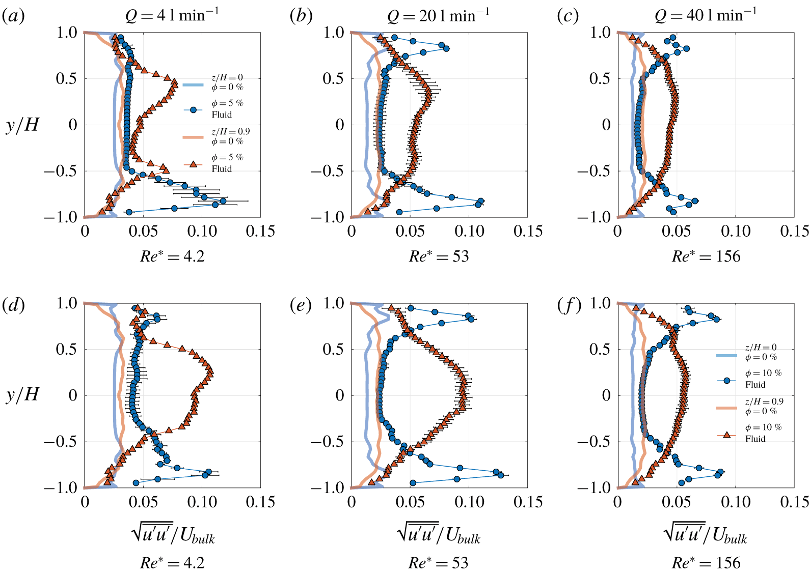
The presence of particles introduces unsteady disturbances in the surrounding fluid field. The streamwise and wall-normal components of the velocity fluctuations associated with these disturbances are displayed in figures 16 and 17, following the same scheme as in the last two figures, as also detailed in the captions. Compared to the single-phase case, the streamwise and wall-normal fluctuations are higher. For the lowest flow rates, sedimentation causes rather high streamwise fluctuations at the bottom of the centre plane (see  $z/H=0$ in figures 16a and 16d).
At higher flow rates, the fluctuation profiles become increasingly symmetric. Considering the duct centre plane, streamwise fluctuations reach peak values close to the top and bottom walls, which are also the locations of high particle concentration. Interestingly, the fluctuations are higher for the intermediate  $Re^{\ast }=53$ than at higher $Re^{\ast }=156$. This is perhaps the result of particles arranging themselves in an intermediate configuration between accumulations at the corners observed at low flow rates and the ring-like structure of the high flow rates. In other words, at such $Re^{\ast }$, the spread of the particles in the duct is higher as also illustrated in figure 13 and hence for the same $\unicode[STIX]{x1D719}$, the unsteadiness in the fluid field is larger. At higher flow rates, most of the particles cluster near the wall bisectors, the frequency of particles passing in this region is increased and hence, the unsteadiness in the velocities, or departure from the mean velocity, is not so pronounced leading to lower root mean square values in the near-wall planes. Measurements at additional planes will be needed to prove the above qualitative picture; nevertheless, the presence of increased streamwise disturbances in the presence of particles is clearly demonstrated.
Change of wall-normal velocity fluctuations due to introduction of particles at two spanwise planes:  $z/H=0$ (centre plane) and $z/H=0.9$ (plane close to the side wall). Panels (a–c) corresponds to $\unicode[STIX]{x1D719}=5\,\%$ and panels (d–f) corresponds to $\unicode[STIX]{x1D719}=10\,\%$.
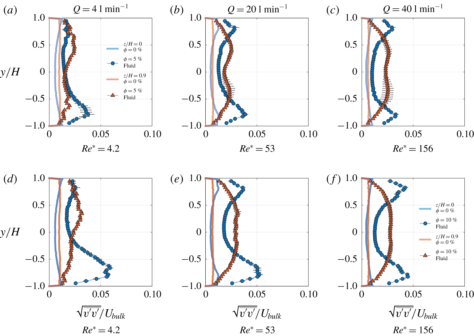
The appearance of streamwise fluctuations is also accompanied by wall-normal velocity fluctuations, as depicted in figure 17. Settling of particles at lower flow rates (refer to figures 17a and 17d) leads to higher wall-normal fluctuations near the bottom of the duct while at the highest flow rates, the profiles are symmetric with nearly the same magnitudes for the two highest  $Re^{\ast }$ (compare figure 17b–17c and 17e–17f).
Reynolds shear stress due to the introduction of particles at two spanwise planes for multiple flow rates (or  $Re^{\ast }$) and both $\unicode[STIX]{x1D719}=5$ and 10 %. The single-phase reference case is also shown (solid lines) for comparison. Note that the limits of the $x$-axis are local to each plot corresponding to a fixed flow rate.

Set-up for shadowgraph imaging. The streamwise direction is out of the plane of the paper.

Despite the presence of intense streamwise and wall-normal fluid velocity fluctuations, the correlation between these two components, i.e. the Reynolds shear stress  $\overline{u^{\prime }v^{\prime }}$, does not drastically increase when compared to the corresponding single-phase case, as shown in figure 18. For reference, the peak values of $\overline{u^{\prime }v^{\prime }}/{U^{2}}_{Bulk}$ in Newtonian turbulence is approximately $3{-}5\times 10^{-3}$. Thus, the fluctuations generated in the flow are not a signature of the classical turbulence in a duct distinguished by a larger Reynolds shear stress, but is an unsteady flow perturbed by solid particles.
4 Discussion
In order to shed more light on the overall particle distribution in the duct, the quantitative measurements in figure 14 are complemented by flow visualisations obtained with shadowgraphy experiments. The set-up is sketched in figure 19, where the duct is illuminated by a point source of light such as an LED. The slight non-uniformity in the refractive index created by the particles inside the suspending medium casts a magnified shadow over the entire volume of a section of the duct on a screen, observable in a dark room. This shadow is captured by a camera, as shown in figure 20.
The qualitative visualisation in figures 20(b) and 20(d), corresponding to the fully developed flow, along with the quantitative concentration profiles from figure 14, are used to sketch an approximate particle distribution pattern at low and high flow rates, see figures 21(a) and 21(b). The increased particle concentration near the bottom wall for low flow rates, due to gravitational forces, is also reproduced in figure 21(a). For consistency, the same number of particles is depicted in both the figures. Note also that visualisations in additional planes besides those reported in figure 14 using the PIV laser sheet have contributed to draw the sketches in figure 21.
Visualisation of particle distribution at the entrance ( $x/H\approx 12$; a,c) and far downstream ( $x/H\approx 160$; b,d) in the duct at both low $(Q=4~\text{l}~\text{min}^{-1})$ and high $(Q=40~\text{l}~\text{min}^{-1})$ flow rates, using simple shadowgraphs. Note: the PIV–PTV measurements were performed at $x/H\approx 150$.

Schematic of the particle distribution in the cross-stream section of the duct. The arrows and streamlines representing the normalised secondary flow and the extent of the plug are from the actual experimental measurements for single-phase flow at the corresponding flow rates. The contours represent the streamwise velocity normalised by the bulk velocity. Note that the colour bar is the same as in figure 10. The particle distribution is schematically reconstructed from the shadowgraphs and PIV measurements.

In order to explain the observed concentration distribution, it is essential to acknowledge the presence of competing forces of an inertial and viscoelastic nature. Scaling analysis can be used to demonstrate the significance of the different forces. In a fluid without elasticity, when the Reynolds number at the particle scale  $Re_{p,\dot{\unicode[STIX]{x1D6FE}}}=\unicode[STIX]{x1D70C}\dot{\unicode[STIX]{x1D6FE}}(d_{p}/2)^{2}/\unicode[STIX]{x1D707}_{f}$ becomes ${\geqslant}1$, the shear gradient lift forces $F_{L}\propto \unicode[STIX]{x1D70C}_{f}\dot{\unicode[STIX]{x1D6FE}}^{2}{d_{p}}^{4}$ (Asmolov Reference Asmolov1999) will push the particle away from the core, whereas the repulsive wall forces will act to displace the particle away from the walls. As a result, an isolated particle reaches a stable equilibrium position somewhere in between the centre and the wall, a phenomenon famously known as the Segré–Silberberg effect (Segre & Silberberg Reference Segre and Silberberg1961). In a square duct, due to repulsion from adjacent orthogonal walls, the stable equilibrium position is at the centre of the walls (Stoecklein & Di Carlo Reference Stoecklein and Di Carlo2018). In our experiments, the maximum value of $Re_{p,\dot{\unicode[STIX]{x1D6FE}}}$ occurs at the wall and is estimated to be ${\approx}0.1$ at $2~\text{l}~\text{min}^{-1}$, and ${\approx}6$ at $40~\text{l}~\text{min}^{-1}$ for $LYS$ fluid flow. Thus, for the lower flow rates the inertial migration towards the centre of the wall is estimated to be very weak. On the other hand, one can estimate the relative magnitudes of viscoelastic forces $F_{VE}\propto (N_{1}+2N_{2}){d_{p}}^{2}$ (see D’Avino et al. Reference D’Avino, Romeo, Villone, Greco, Netti and Maffettone2012). From De Cagny et al. (Reference De Cagny, Fazilati, Habibi, Denn and Bonn2019), the normal-stress differences can be approximated as ${\sim}\unicode[STIX]{x1D70F}^{2}/G^{\prime }$. Thus, $F_{L}/F_{VE}\propto (G^{\prime }\unicode[STIX]{x1D70C}_{f}{d_{p}}^{2})/(\unicode[STIX]{x1D70F}/\dot{\unicode[STIX]{x1D6FE}})^{2}$. For a given flow rate, the force ratio is maximum at the wall since the denominator is some form of apparent viscosity that should be lowest at the wall. Thus, if the wall-shear stress $\unicode[STIX]{x1D70F}_{w}=\unicode[STIX]{x1D70F}_{y}/Bi$ and a nominal shear rate $\dot{\unicode[STIX]{x1D6FE}}=U_{Bulk/H}$ are used to evaluate the above force ratio, it ranges from $10^{-2}$, for the lowest flow rate to $1$, for the highest flow rate. This indicates the relative dominance of viscoelastic forces over inertial lift forces at the lowest flow rates. It also explains why particles migrate towards the corners (see illustration in figure 21a) which is a typical behaviour in inertialess $(Re_{p}\sim 0)$ viscoelastic fluids (Villone et al. Reference Villone, D’avino, Hulsen, Greco and Maffettone2013), compared to inertial migration towards the centre of the walls in a square geometry. The observed migration is, in particular, due to the non-uniform distribution of the first normal-stress difference, being maximum at the wall centre and minimum at the corners and core (Yang et al. Reference Yang, Kim, Lee, Lee and Kim2011). Migration towards the core is not as pronounced due to the presence of the non-yielded core with its infinite viscosity. Hence, the non-zero concentration inside the plug is most likely due to particles that were trapped in the bulk at the inlet to the duct.
With increasing flow rates,  $Re_{p}$ as well as $F_{L}/F_{VE}$, increases i.e. inertia starts to affect the migration and drives the particles to the centre of the walls. However, our experimental measurements and shadowgraphy observations show that, instead of being concentrated only at the wall centres, the particle distribution is similar to that sketched in figure 21(b). Thus, we have reason to believe that, in addition to inertial migration, the particle distribution is also influenced by the increasing intensity of secondary flow, induced by the second normal-stress differences. The competition between the first normal-stress driven migration and secondary flow driven migration was already explored in Villone et al. (Reference Villone, D’avino, Hulsen, Greco and Maffettone2013), who found that with increasing flow rates, the velocity of the secondary flow increases faster than the migration velocity due to first normal-stress differences. As a consequence, particles may now also be dragged by the helicoidal motion of the secondary flow (also see Lim, Nam & Shin (Reference Lim, Nam and Shin2014b)). The secondary flow measured for the single-phase cases is most likely changed by the presence of the particles; however, it is not reported in this study since measurements displayed excessive noise and showed consistent behaviour. Nonetheless, in a Newtonian suspending medium, the modifications of the secondary flow due to cross-stream migration of finite-size particles in a square duct have been shown in numerical studies as in Kazerooni et al. (Reference Kazerooni, Fornari, Hussong and Brandt2017). Previously, Ramachandran & Leighton (Reference Ramachandran and Leighton2008) proved that strong secondary normal-stress differences, and hence secondary flows, can be produced in concentrated suspensions due to an anisotropic particle microstructure. Finally, due to high local concentration and non-negligible $Re_{p}$ at high flow rates, multi-particle interactions may also influence particle dispersion. Non-negligible $Re_{p}$ at higher flow rates may lead to inertial effects like shear thickening (Picano et al. Reference Picano, Breugem, Mitra and Brandt2013), which can influence the friction factor. We note that in our experiments at the higher flow rates, the plug in the core has a negligible size or is perhaps non-existent, and the flow therefore approaches the case of particles in a shear-thinning viscoelastic fluid.
The simple shadowgraphy visualisations also help in assessing the evolution of the particle distribution along the duct streamwise length. Figures 20(a) and 20(c) show the shadowgraphs of the particle distribution very close to the entrance of the duct (at  $x/H\approx 12$) at low and high flow rates. At the low flow rate, particles seem to enter the duct while being mostly concentrated in the bottom half. This entry profile may either be due to gravitational forces or because of the secondary Dean motion from the bend at the exit of the tank in our set-up. The installed static mixer meant to cancel these vortices is, perhaps, less effective at such low $Re^{\ast }$. Nevertheless, as the flow develops, the initial disturbances are dissipated and particles attain an equilibrium concentration, as shown in figure 20(b), which is captured very close to the location where the PIV measurements are performed. Thus, particles migrate to the top against gravitational forces. Particles travelling at a higher speed in the core are seen to move without any change in their relative positions on account of being locked up inside the solid plug. On many occasions, clusters of two or more particles are seen to move together inside the plug (which was observed before in the case of particle sedimentation by Chaparian, Wachs & Frigaard (Reference Chaparian, Wachs and Frigaard2018)). The distribution profile just described is attained much earlier than $x/H\approx 160$ and persists along the remaining length of the duct. Projection from only one direction is insufficient to give full information on the particle distribution and, hence, the duct was also illuminated from the bottom to check a second projection. And indeed, a picture very similar to that in figure 20(b) is obtained, thus confirming the preferential accumulation of particles at the corners.
Focussing on the highest flow rates, it appears that the concentration profile is more uniform at the entrance (see figure 20c) and rapidly develops to an equilibrium pattern, as seen in figure 20(d). By visualising fast and slow particles, it appears that very few particles travel near the core, which has the highest velocity, or at the corners, which have the smallest velocity. Most of the particles travel in the intermediate region between the core and the corners. Moreover, the particle motion appears very erratic with instances of rapid change in their velocities. This indicates that strong particle–particle and particle–wall interactions are most likely relevant at these concentrations and flow rates. The presence of finite-size particles also causes an increase in the local strain rates, and the corresponding reduction in the local viscosity for the shear-thinning fluid may intensify the strength of these interactions, which may be an important mechanism for generating the fluid velocity fluctuations shown in figures 16 and 17.
To conclude, we note that from a visualisation perspective, another noteworthy technique can be used, exploiting the property of elastoviscoplastic flows to come to a rather quick stop after switching off the pump, as mentioned earlier. As a result, the particles get trapped in their flowing configuration without much change of the inter-particle distance, thus making it possible to assess their position and hence, the concentration distribution. This can be conveniently done by translating the laser sheet across such a frozen flow and capturing still photos which can be later stacked together to reconstruct the full three-dimensional concentration field. Such experiments are not performed here but can be advantageously used for these kinds of fluids.
5 Conclusion
We have presented an experimental study of the flow of an elastoviscoplastic fluid, Carbopol gel, at two different concentrations – one with a high yield stress and the other with a low yield stress – and studied the laminar single-phase flow and the flow in the presence of finite-size spherical particles at relatively high concentrations inside a square duct. Pressure drop, mean and fluctuating velocities and concentration fields have been measured using a combination of PIV and PTV; these optical techniques have been possible due to the refractive-index matching of the fluid–particle mixture. To facilitate comparative simulations, the rheological properties of the fluids investigated are described in terms of the steady-state flow curves and viscoelastic moduli. A measure of normal-stress differences is provided from the recent work of De Cagny et al. (Reference De Cagny, Fazilati, Habibi, Denn and Bonn2019).
The experimental pressure drop is in agreement, over the range of flow rates considered, with the laminar friction factor based on the semi-empirical Reynolds number  $Re^{\ast }$ (see (1.1)) by Liu & Masliyah (Reference Liu and Masliyah1998). By making use of the symmetries in a square duct, we have presented the full 3-component velocity field (at moderate spatial resolution) for single-phase flow using two-dimensional PIV in multiple spanwise planes (at high spatial resolution), evidencing the existence of a secondary flow due to the viscoelastic properties of the fluid after yielding. Using a low threshold value of the velocity gradient, we have identified the near-circular plug region in the core, whose size reduces with increasing the flow rate or equivalently $Re^{\ast }$. At the same $Re^{\ast }$, the fluid with a higher yield stress has a higher Bingham number $Bi$ and a larger plug. Also, at the same $Bi$, the ratio of the maximum streamwise velocity to the bulk velocity is larger for a fluid with a higher power law exponent $n$. The strength and size of the streamwise vortices representing the secondary flow increases for reducing plug sizes. Shear thinning and secondary flow cause a deviation of the mean streamwise velocity when compared with the simulations of Saramito & Roquet (Reference Saramito and Roquet2001) for a Bingham fluid.
Similar to Newtonian suspending fluids, the friction factor increases by increasing the particle volume fraction  $\unicode[STIX]{x1D719}$ at fixed $Re^{\ast }$. This increase seems independent of the rheology of the suspending fluid. A reasonably good prediction is obtained based on the effective viscosity of suspensions of rigid spheres in Newtonian fluid, like the Eilers fit. The matching with predictions based on the rheological modifications of YSF proposed by Chateau et al. (Reference Chateau, Ovarlez and Trung2008) is not so good. These differences are most likely due to a non-uniform particle distribution in the duct, which violates the assumptions of the above theory. At low flow rates, in the presence of a larger plug and weaker secondary flow, particles migrate inside the yielded zone, defying gravity, towards the four corners under the influence of the first normal-stress difference. Fluid (and particle) velocity reduces in the near-wall planes (where there is a high particle concentration) and increases in the plane of the wall bisector when compared to the corresponding single-phase flow at the same locations. This increase of the maximum velocity reflects in an increased shear in the core region and results in a smaller plug than for the single-phase flow. At high flow rates, in the presence of a negligibly small plug and a stronger secondary flow and inertial lift forces, particles arrange along a diffused ring between the core and the corners. A simple scaling of forces is provided to explain the dominance of viscoelastic forces at low flow rates and inertial forces at high flow rates. Particles are also seen to induce time-dependent fluid velocities, leading to uncorrelated fluctuations in the streamwise and wall-normal directions. Visualisation of shadowgraphs have, even though qualitatively, confirmed the above concentration profiles.
The importance and novelty of this experiment, when compared to other studies with particles in non-Newtonian fluids, is the ability to assess the velocity distribution of both the fluid and particle phases along with particle distribution at high bulk concentrations. This will, hopefully, help in future modelling attempts of such systems and shed light on the complex fluid–particle interactions present therein. These results are especially relevant to microfluidic applications, which share similar values of the relevant non-dimensional parameters, e.g. the Reynolds number  $Re^{\ast }$ and confinement (or blockage) ratios and where resolved measurements are prohibited by the small length scales. As always, further investigation with different particle sizes, volume fractions and fluid rheologies, perhaps coupled with spatio-temporally resolved measurements, will help to further understand these complex systems.
Acknowledgements
This work was supported by the European Research Council grant no. ERC-2013-CoG-616186, TRITOS, from the Swedish Research Council (VR), through the Outstanding Young Researcher Award to L.B. Å. Engström (Rise Bioeconomy AB) is gratefully acknowledged for assistance with the rheological measurements. The velocity field data are available in Zade et al. (Reference Zade, Shamu, Lundell and Brandt2019c).


 Open access