


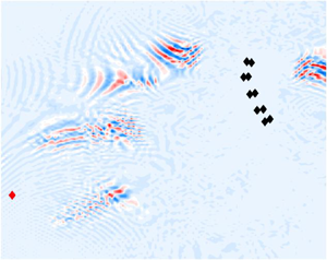



1. Introduction
Tsunamis are long-wavelength surface–gravity waves that can cause significant loss of life and damage to property. Recent examples include 2011 Tohoku Oki; 2018 Sulawesi; Palu, Tonga 2022; and the deadliest event so far recorded, the 2004 Sumatra tsunami. Given that tsunamigenic events cannot yet be predicted ahead of time, present-day efforts are directed towards providing early warning systems to mitigate the worst consequences of facing an oncoming tsunami. Existing early warning systems make use of data received from DART (deep ocean assessment and reporting of tsunamis) buoys and seismic measurements. The DART buoys are capable of assessing a tsunami threat, but under standard circumstances, may not leave much time for early warning. Seismic sources can provide information on earthquake size, epicentre etc., but do not comment on possible tsunami characteristics. Tsunamis can be generated by any process that displaces a large volume of water such as volcanic activity, landslides, meteorite strikes and undersea earthquakes. Taking the undersea earthquake as an example, the vertical uplift in the seabed (rupture) elevates and slightly compresses the water column above the rupture zone. Under the restoring force of gravity, fast-moving surface–gravity waves, the tsunami, propagate away from the epicentre at relatively high speed, e.g.  $\simeq 200\ {\rm m s}^{-1}$ in 4000 m deep water. The compression of the water column above the rupture zone generates low-frequency sound waves, known as acoustic–gravity waves, that propagate at much higher speed ( $\simeq 1450\ {\rm s}^{-1}$) and are able to outrun the tsunami in the far field. Acoustic–gravity waves can couple to the elastic seabed and double their speed (Kadri Reference Kadri2019) and in the solid medium of the seabed compression $P$ waves and shear $S$ waves can propagate at speeds of $\simeq 6800\ {\rm m s}^{-1}$ and $\simeq 3550\ {\rm m s}^{-1}$, respectively (Dziewonshi & Anderson Reference Dziewonshi and Anderson1981). However the acoustic–gravity waves in the liquid layer are directly linked to the effective uplift of the rupture zone and thus encode information regarding the rupture geometry and dynamics. In this way the acoustic–gravity waves not only provide a possible means of early detection, but also are a reliable source of information. This information can be extracted, and utilised via an inverse process to determine rupture characteristics (Mei & Kadri Reference Mei and Kadri2018; Gomez & Kadri Reference Gomez and Kadri2021).
Previous work studied the possibility of using acoustic–gravity waves as early warning signals (Yamamoto Reference Yamamoto1982; Nosov Reference Nosov.1999; Stiassnie Reference Stiassnie2010; Renzi & Dias Reference Renzi and Dias2014; Kadri Reference Kadri2015, Reference Kadri2016). In these studies the rupture zone has been modelled in a variety of ways (infinite strip, oscillating block, cylinder) and the seabed is normally considered rigid. However, for those cases where the shape of the rupture can be modelled as a rectangular slender body (table 1 of Mei & Kadri Reference Mei and Kadri2018) multiple-scales analysis can be applied to take advantage of the differing length scales of the fault. Within Mei & Kadri (Reference Mei and Kadri2018) the primary focus was on pure acoustic waves, ignoring gravitational effects, whereas a later work (Williams, Kadri & Abdolali Reference Williams, Kadri and Abdolali2021) extended the derivations to include gravity and therefore captured the behaviour of the surface–gravity waves in addition to the acoustic–gravity waves. Moreover, the slender-fault model was applied to more complex, multi-fault scenarios, such as the 2016 Kaikoura earthquake (Hamling et al. Reference Hamling2016), via linear superposition – but still with a rigid seabed. However, the elastic properties of the solid medium should not always be ignored (Abdolali, Kadri & Kirby Reference Abdolali, Kadri and Kirby2019; Kadri Reference Kadri2019) since the water compressibility and seabed elasticity affect the phase speed of surface waves, and thus the arrival times of transoceanic tsunamis (Abdolali et al. Reference Abdolali, Kadri and Kirby2019). A complementary work by Eyov et al. (Reference Eyov, Klar, Kadri and Stiassnie2013) investigated the consequences of imposing an elastic seabed as support for a liquid layer residing in a gravitational field upon the form of the dispersion relation. The inclusion of an elastic seabed allows acoustic–gravity waves propagating in shallower water before dissipating into the elastic medium. In stark contrast to the rigid-seabed case the first acoustic mode is able to propagate as a Scholte wave to the shore, where it turns into a Rayleigh wave (Eyov et al. Reference Eyov, Klar, Kadri and Stiassnie2013). Note that no rupture was considered in Eyov et al. (Reference Eyov, Klar, Kadri and Stiassnie2013). The primary objective of this paper is to combine the ground movement of rectangular slender faults with an elastic seabed, in order to study the contribution of elasticity to the propagation of both acoustic–gravity waves and surface waves. The results of this paper should help fill a gap in the literature identified within Renzi (Reference Renzi2017) in which the authors claim solutions for acoustic–gravity waves produced by disturbances over an elastic seabed in three dimensions are missing from the literature.
Another difference encountered when studying the elastic case is that rather than the single surface–gravity wave (found in rigid seabed analysis) there is now the possibility of two surface–gravity waves (Eyov Reference Eyov2013). There is the usual tsunami (referred to there as mode 01), and another mode of much smaller amplitude which does not propagate for all frequencies (referred to here as mode 00 (Eyov Reference Eyov2013)). Other secondary objectives include deriving improved estimates for the acoustic–gravity wave critical frequencies, estimating the cut-off frequency for the second surface wave (mode 00), and presentation of a method for rapid calculation of approximate phase velocity curves. We ignore terms of second order and higher (i.e. nonlinear terms) since the free-surface displacements are small in comparison with the water depth (Yoon Reference Yoon2002), and also small in comparison with the wavelengths considered (Michele & Renzi Reference Michele and Renzi2020). In addition the gravity term that is present in the full wave equation is omitted because its contribution is small (see figure 2 of Abdolali et al. Reference Abdolali, Kadri and Kirby2019).
This paper comprises seven main sections. The mathematical formulation combining ground movement with elasticity is found in § 2, with its solution in § 3. Section 4 presents improved approximations for the acoustic–gravity wave cut-off frequencies, and an estimate of the cut-off frequency for the mode 00 surface wave. Section 5 proposes a method for fast calculation of approximate phase velocity curves which does not necessitate solution of the dispersion relation at each data point. Section 6 links the developed theory to numerical results obtained from both synthetic stimulus and real data from hydrophones and DART buoys. The paper concludes with a discussion/summary in § 7.
2. Formulation
The water layer is considered inviscid, homogeneous, of constant depth  $h$, residing in a gravitational field of constant acceleration $g=9.81\ {\rm m s}^{-1}$. The water layer is assumed unbounded in $x$ and $y$ and is supported by an infinitely deep elastic half-space. The origin of coordinates is taken at the unperturbed free surface directly above the centroid of the slender fault, with the $z$ axis pointing vertically upwards. Assuming irrotational flow, the problem is expressed in terms of a velocity potential function for the liquid $\phi _{l}$, along with a dilation potential $\phi _{s}$ and rotation potential $\boldsymbol {\varPsi }$ for the solid layer (the subscript $s$ is omitted from $\boldsymbol {\varPsi }$ since it only exists in the solid). As in Eyov et al. (Reference Eyov, Klar, Kadri and Stiassnie2013) we make use of linearised, irrotational flow for the liquid and linear elasticity for the solid. A representation of the flow domain is given in figure 1(a) with a top view of the slender fault in figure 1(b). With $\boldsymbol {i}, \boldsymbol {j}, \boldsymbol {k}$ as unit vectors the velocity in the liquid is given by
 \begin{equation} \dot{\boldsymbol{U}_{l}}={-}\boldsymbol{\nabla}\phi_{l}= \dot{u}_{l}\boldsymbol{i}+\dot{v}_{l}\boldsymbol{j}+ \dot{w}_{l}\boldsymbol{k}={-}\frac{\partial\phi_{l}}{\partial x}\boldsymbol{i}-\frac{\partial\phi_{l}}{\partial y}\boldsymbol{j}-\frac{\partial\phi_{l}}{\partial z}\boldsymbol{k}. \end{equation}
The solid displacements are then
 $$\begin{gather} \boldsymbol{U}_{s}=\boldsymbol{\nabla}\phi_{s}+ \boldsymbol{\nabla}\times\boldsymbol{\varPsi}=u_{s} \boldsymbol{i}+v_{s}\boldsymbol{j}+w_{s}\boldsymbol{k}, \end{gather}$$
 $$\begin{align}u_{s}=\frac{\partial\phi_{s}}{\partial x}+ \left(\frac{\partial\psi_{z}}{\partial y}- \frac{\partial\psi_{y}}{\partial z}\right), \quad v_{s}=\frac{\partial\phi_{s}}{\partial y}+ \left(\frac{\partial\psi_{x}}{\partial z}-\frac{\partial \psi_{z}}{\partial x}\right), \quad w_{s}=\frac{\partial\phi_{s}}{\partial z}+ \left(\frac{\partial\psi_{y}}{\partial x}- \frac{\partial\psi_{x}}{\partial y}\right). \end{align}$$
The potentials are governed by three wave equations. In the liquid region:
 \begin{equation} \frac{\partial^{2}\phi_{l}}{\partial x^{2}}+\frac{\partial^{2}\phi_{l}}{\partial y^{2}}+\frac{\partial^{2}\phi_{l}}{\partial z^{2}}=\frac{1}{C_{l}^{2}}\frac{\partial^{2}\phi_{l}}{\partial t^{2}}, \quad -h\leq z\leq0, \end{equation}
where  $C_{l}$ is the speed of sound in water. In the solid region:
 $$\begin{gather} \frac{\partial^{2}\phi_{s}}{\partial x^{2}}+\frac{\partial^{2}\phi_{s}}{\partial y^{2}}+\frac{\partial^{2}\phi_{s}}{\partial z^{2}}=\frac{1}{C_{p}^{2}}\frac{\partial^{2}\phi_{s}}{\partial t^{2}}, \quad z\leq{-}h, \end{gather}$$
 $$\begin{gather}\frac{\partial^{2}\boldsymbol{\varPsi}}{\partial x^{2}}+\frac{\partial^{2}\boldsymbol{\varPsi}}{\partial y^{2}}+\frac{\partial^{2}\boldsymbol{\varPsi}}{\partial z^{2}}=\frac{1}{C_{s}^{2}}\frac{\partial^{2}\boldsymbol{\varPsi}}{\partial t^{2}}, \quad z\leq{-}h, \end{gather}$$
where  $C_{p}$ and $C_{s}$ are the pressure and shear wave velocities respectively:
 \begin{equation} C_{p}=\sqrt{\frac{1}{\rho_{s}}(\lambda+2\mu)}, \quad C_{s}=\sqrt{\frac{\mu}{\rho_{s}}}, \end{equation}
where  $\lambda, \mu$ are Lamé constants and $\rho _{s}$ is the density of the solid. At the free surface we have the combined kinematic and dynamic boundary condition:
 \begin{equation} \frac{\partial^{2}\phi_{l}}{\partial t^{2}}+g\frac{\partial\phi_{l}}{\partial z}=0, \quad z=0. \end{equation}
In addition, there are four boundary conditions for the seabed. The first of these ensures the vertical component of velocity in the liquid matches that of the solid. The component  $w_{s}$ is the vertical component of the seabed motion when there is no rupture (as studied in Eyov et al. (Reference Eyov, Klar, Kadri and Stiassnie2013)) and as such is small (however, ${\partial w_{s}}/{\partial t}$ may not be). The magnitude of $w_{s}$ ranges from $10^{-6}$ m for microseisms to $10^{-2}$ m for severe earthquakes (Eyov et al. Reference Eyov, Klar, Kadri and Stiassnie2013).
 \begin{equation} \dot{w}_{l}=\frac{\partial w_{s}}{\partial t}+W(x,y,t), \quad z={-}h. \end{equation}
The definition of  $W(x,y,t)$ closely follows that in (3.2a,b) of Mei & Kadri (Reference Mei and Kadri2018) and describes the motion of the rupture:
 $$\begin{gather} W(x,y,t)=R(x,y)\tau(t), \quad z={-}h, \end{gather}$$
 $$\begin{gather}R(x,y)=\begin{cases} W_{0}=\text{const.} & |x|< b, \,|Y|< {\unicode{x00A3}}\\ 0 & \text{elsewhere}, \end{cases} \quad \tau(t)=\begin{cases} 1 & -T< t< T\\ 0 & |t|>T, \end{cases} \quad {\unicode{x00A3}}=\epsilon L. \end{gather}$$
The duration of the rupture is  $2T$, the slender fault half-width is $b$ and the slender fault half-length is $L$. The slenderness parameter is then $\epsilon ={b}/{L} \ll 1$ (see figure 1b). Note that if there is no rupture, i.e. $W(x,y,t)=0$, then the boundary condition (2.9) reduces to that of (8a) of Eyov et al. (Reference Eyov, Klar, Kadri and Stiassnie2013), $\dot {w}_{l}={\partial w_{s}}/{\partial t}$. On the other hand, when the seabed is rigid, $w_{s}=0$, and we recover the bottom boundary condition (2.3) of Mei & Kadri (Reference Mei and Kadri2018), $\dot {w}_{l}=W(x,y,t)=-{\partial \phi _{l}}/{\partial z}$, but this time with a minus sign due to this paper following the sign choices in (1a) and (1b) of Eyov et al. (Reference Eyov, Klar, Kadri and Stiassnie2013).
Representation of the flow domain. (a) Cross-section through the  $x, z$ plane. Water depth is $h$, surface elevation is $\eta (x,y,t)$, liquid velocity potential is $\phi _{l}$, solid dilation potential is $\phi _{s}$ and solid rotation potential is $\boldsymbol {\varPsi }$. Densities in the liquid and solid medium are $\rho _{l}$ and $\rho _{s}$ respectively. (b) Top view of slender fault.

The next boundary condition states that the axial stress  $\sigma _{zz}$ is equal in magnitude but of opposite direction to the liquid pressure at the seabed:
 $$\begin{gather} \sigma_{zz}={-}P_{l}, \quad z={-}h, \end{gather}$$
 $$\begin{gather}\sigma_{zz}=\lambda\left(\frac{\partial u_{s}}{\partial x}+\frac{\partial v_{s}}{\partial y}+\frac{\partial w_{s}}{\partial z}\right)+2\mu\frac{\partial w_{s}}{\partial z}={-}P_{l}, \quad z={-}h. \end{gather}$$
The remaining two boundary conditions define no shear on the seabed:
 \begin{equation} \sigma_{xz}=0,\quad\sigma_{yz}=0,\quad z={-}h, \end{equation}
so that
 \begin{equation} \sigma_{xz}=\mu\left(\frac{\partial u_{s}}{\partial z}+\frac{\partial w_{s}}{\partial x}\right)=0,\quad \sigma_{yz}=\mu\left(\frac{\partial v_{s}}{\partial z}+\frac{\partial w_{s}}{\partial y}\right)=0,\quad z={-}h. \end{equation}
The dynamic pressure and surface elevation are obtained from
 \begin{equation} P_{l}=\rho_{l}\frac{\partial\phi_{l}}{\partial t}, \quad \eta=\frac{1}{g}\frac{\partial\phi_{l}}{\partial t}. \end{equation}
We also require  $\phi _{l}, \phi _{s},\boldsymbol {\varPsi }$ and all derivatives to decay to zero as $x,y,t\rightarrow \pm \infty, z\rightarrow -\infty$.
3. Solution
We introduce multiple-scale coordinates following Mei & Kadri (Reference Mei and Kadri2018):
 \begin{equation} x, z, t; \quad X=\epsilon^{2}x, \quad Y=\epsilon y. \end{equation}
The wave equations (2.4)–(2.6) can then be written as
 $$\begin{gather} \frac{\partial^{2}\phi_{l}}{\partial x^{2}}+2\epsilon^{2}\frac{\partial^{2}\phi_{l}}{\partial x\partial X}+\epsilon^{2}\frac{\partial^{2}\phi_{l}}{\partial Y^{2}}+\frac{\partial^{2}\phi_{l}}{\partial z^{2}}=\frac{1}{C_{l}^{2}}\frac{\partial^{2}\phi_{l}}{\partial t^{2}}, \quad -h\leq z\leq0, \end{gather}$$
 $$\begin{gather}\frac{\partial^{2}\phi_{s}}{\partial x^{2}}+2\epsilon^{2}\frac{\partial^{2}\phi_{s}}{\partial x\partial X}+\epsilon^{2}\frac{\partial^{2}\phi_{s}}{\partial Y^{2}}+\frac{\partial^{2}\phi_{s}}{\partial z^{2}}=\frac{1}{C_{p}^{2}}\frac{\partial^{2}\phi_{s}}{\partial t^{2}}, \quad -\infty\leq z\leq{-}h, \end{gather}$$
 $$\begin{gather}\frac{\partial^{2}\boldsymbol{\varPsi}}{\partial x^{2}}+2\epsilon^{2}\frac{\partial^{2}\boldsymbol{\varPsi}}{\partial x\partial X}+\epsilon^{2}\frac{\partial^{2}\boldsymbol{\varPsi}}{\partial Y^{2}}+\frac{\partial^{2}\boldsymbol{\varPsi}}{\partial z^{2}}=\frac{1}{C_{s}^{2}}\frac{\partial^{2}\boldsymbol{\varPsi}}{\partial t^{2}}, \quad -\infty\leq z\leq{-}h. \end{gather}$$
Let  $\phi _{l}=\phi _{l0}(x,X,Y,z,t)+\epsilon ^{2}\phi _{l2}(x,X,Y,z,t)$, with similar expressions for $\phi _{s}$ and $\boldsymbol {\varPsi }$. Then the perturbation equations at $O(\epsilon ^{0})$ describe the two-dimensional problem of an infinitely long slender fault:
 $$\begin{gather} \frac{\partial^{2}\phi_{l0}}{\partial x^{2}}+\frac{\partial^{2}\phi_{l0}}{\partial z^{2}}-\frac{1}{C_{l}^{2}}\frac{\partial^{2}\phi_{l0}}{\partial t^{2}}=0, \quad -h\leq z\leq0, \end{gather}$$
 $$\begin{gather}\frac{\partial^{2}\phi_{s0}}{\partial x^{2}}+\frac{\partial^{2}\phi_{s0}}{\partial z^{2}}-\frac{1}{C_{p}^{2}}\frac{\partial^{2}\phi_{s0}}{\partial t^{2}}=0, \quad -\infty< z\leq{-}h, \end{gather}$$
 $$\begin{gather}\frac{\partial^{2}\boldsymbol{\varPsi}_{0}}{\partial x^{2}}+\frac{\partial^{2}\boldsymbol{\varPsi}_{0}}{\partial z^{2}}-\frac{1}{C_{s}^{2}}\frac{\partial^{2}\boldsymbol{\varPsi}_{0}}{\partial t^{2}}=0, \quad -\infty< z\leq{-}h. \end{gather}$$
At  $O(\epsilon ^{2})$,
 $$\begin{gather} \frac{\partial^{2}\phi_{l2}}{\partial x^{2}}+\frac{\partial^{2}\phi_{l2}}{\partial z^{2}}-\frac{1}{C_{l}^{2}}\frac{\partial^{2}\phi_{l2}}{\partial t^{2}}={-}\left\{ \frac{\partial^{2}\phi_{l0}}{\partial Y^{2}}+2\frac{\partial^{2}\phi_{l0}}{\partial x\partial X}\right\} , \quad -h\leq z\leq0, \end{gather}$$
 $$\begin{gather}\frac{\partial^{2}\phi_{s2}}{\partial x^{2}}+\frac{\partial^{2}\phi_{s2}}{\partial z^{2}}-\frac{1}{C_{p}^{2}}\frac{\partial^{2}\phi_{s2}}{\partial t^{2}}={-}\left\{ \frac{\partial^{2}\phi_{s0}}{\partial Y^{2}}+2\frac{\partial^{2}\phi_{s0}}{\partial x\partial X}\right\} , \quad -\infty\leq z\leq{-}h, \end{gather}$$
 $$\begin{gather}\frac{\partial^{2}\boldsymbol{\varPsi}_{2}}{\partial x^{2}}+\frac{\partial^{2}\boldsymbol{\varPsi}_{2}}{\partial z^{2}}-\frac{1}{C_{s}^{2}}\frac{\partial^{2}\boldsymbol{\varPsi}_{2}}{\partial t^{2}}={-}\left\{ \frac{\partial^{2}\boldsymbol{\varPsi}_{0}}{\partial Y^{2}}+2\frac{\partial^{2}\boldsymbol{\varPsi}_{0}}{\partial x\partial X}\right\} , \quad -\infty\leq z\leq{-}h. \end{gather}$$
The fault motion, elastic properties and elastic dispersion relation are all captured at  $O(\epsilon ^0)$. Thus, the $O(\epsilon ^2)$ boundary conditions for the liquid layer are those for rigid seabed and no fault motion:
 $$\begin{gather} \frac{\partial^{2}\phi_{l2}}{\partial t^{2}}+g\frac{\partial\phi_{l2}}{\partial z} =0,\quad z=0, \end{gather}$$
 $$\begin{gather}\frac{\partial \phi_{l2}}{\partial z} =0,\quad z={-}h. \end{gather}$$
3.1. Leading-order potential
By the double Fourier transforms  $\bar {\mathcal {F}}= \int _{-\infty }^{\infty }\mathcal {F}\,\textrm {e}^{\textrm {i}\omega t}\textrm {d} t, \bar {\bar {\mathcal {F}}}= \int _{-\infty }^{\infty }\bar {\mathcal {F}}\,\textrm {e}^{-\textrm {i} kx}\textrm {d}\kern0.06em x$, with $\omega$ the angular velocity and $k$ the wavenumber, equations (3.5), (3.6) and (3.7) become
 $$\begin{gather} \frac{\partial^{2}\bar{\bar{\phi}}_{l0}}{\partial z^{2}}+\Bigg(\frac{\omega^{2}}{C_{l}^{2}}-k^{2}\Bigg) \bar{\bar{\phi}}_{l0}=0, \end{gather}$$
 $$\begin{gather}\frac{\partial^{2} \bar{\bar{\phi}}_{s0}}{\partial z^{2}}+\Bigg(\frac{\omega^{2}}{C_{p}^{2}}-k^{2}\Bigg) \bar{\bar{\phi}}_{s0}=0, \end{gather}$$
 $$\begin{gather}\frac{\partial^{2}\bar{\bar{\boldsymbol{\varPsi}}}_{0}}{\partial z^{2}}+\left(\frac{\omega^{2}}{C_{s}^{2}}-k^{2}\right) \bar{\bar{\boldsymbol{\varPsi}}}_{0}=0. \end{gather}$$
Let  $E_{1}, E_{2}, D_{1}, D_{2}$ be unknowns to be solved for. Then the choice exists either to select $r^{2}=({\omega ^{2}}/{C_{l}^{2}}-k^{2})$, with $r\in \mathbb {R}$, leading to a trial solution for $\bar {\bar {\phi }}_{l0}$ in (3.13) of the form $\bar {\bar {\phi }}_{l0}(z)=E_{1}\cos (rz)+E_{2}\sin (rz)$, or to select $r^{2}=(k^{2}-{\omega ^{2}}/{C_{l}^{2}})$, leading to a trial solution of the form $\bar {\bar {\phi }}_{l0}(z)=E_{1}\cos (\textrm {i} rz)+E_{2}\sin (\textrm {i} rz)$, as in (12c) of Eyov et al. (Reference Eyov, Klar, Kadri and Stiassnie2013). To maintain compatibility with Eyov et al. (Reference Eyov, Klar, Kadri and Stiassnie2013) we choose $r^{2}=(k^{2}-{\omega ^{2}}/{C_{l}^{2}})$. For (3.14) and (3.15) we take $q^{2}=(k^{2}-{\omega ^{2}}/{C_{p}^{2}})$ and $s^{2}=(k^{2}-{\omega ^{2}}/{C_{s}^{2}})$. As in Eyov et al. (Reference Eyov, Klar, Kadri and Stiassnie2013), $r, q$ and $s$ are wavenumbers.
To arrive at a trial solution for (3.14) we choose  $\bar {\bar {\phi }}_{s0}(z)=D_{1}\,\textrm {e}^{qz}$, because $\bar {\bar {\phi }}_{s0}(z)\rightarrow 0$ as $z\rightarrow -\infty$ implies no terms involving $\textrm {e}^{-qz}$. By a similar argument $\bar {\bar {\boldsymbol {\varPsi }}}_{0}(z)=D_{2}\,\textrm {e}^{sz}\boldsymbol {j}$.
Applying the double Fourier transforms to the boundary condition at  $z=0$ (leading-order term):
 \begin{equation} \frac{\partial^{2}\phi_{l0}}{\partial t^{2}}+g\frac{\partial\phi_{l0}}{\partial z}=0, \quad z=0. \end{equation}
After both Fourier transforms equation (3.16) becomes
 \begin{equation} -\omega^{2}\bar{\bar{\phi}}_{l0}+g \frac{\partial\bar{\bar{\phi}}_{l0}}{\partial z}=0, \quad z=0. \end{equation}
Applying Fourier transforms to the first boundary condition at  $z=-h$ (2.9), leading-order terms become
 $$\begin{gather} w_{s0}=\frac{\partial\phi_{s0}}{\partial z}+ \frac{\partial\psi_{0y}}{\partial x} \quad \text{and} \quad \dot{w}_{l0}={-}\frac{\partial\phi_{l0}}{\partial z}, \end{gather}$$
 $$\begin{gather}-\frac{\partial\phi_{l0}}{\partial z}=\frac{\partial^{2}\phi_{s0}}{\partial t\partial z}+\frac{\partial^{2}\psi_{0y}}{\partial t\partial x}+W(x,y,t). \end{gather}$$
It is only necessary to apply the relevant transforms to the first three terms of (3.19) – the required transforms for  $W(x,y,t)$ are already known from Mei & Kadri (Reference Mei and Kadri2018). Assembling terms gives
 \begin{equation} -\frac{\partial\bar{\bar{\phi}}_{l0}}{\partial z}={-}\textrm{i}\omega\frac{\partial\bar{\bar{\phi}}_{s0}}{\partial z} +\omega k\bar{\bar{\psi}}_{0y}+ \frac{4W_{0}\sin(kb)\sin(\omega T)}{k\omega}, \quad z={-}h. \end{equation}
The second boundary condition at  $z=-h$ is $\sigma _{zz}=-P_{l}$:
 \begin{equation} \sigma_{zz}=\lambda\left(\frac{\partial u_{s0}}{\partial x}+\frac{\partial w_{s0}}{\partial z}\right)+2\mu\frac{\partial w_{s0}}{\partial z}={-}P_{l0}={-}\rho_{l}\frac{\partial\phi_{l0}}{\partial t}, \end{equation}
with
 \begin{equation} u_{s0}=\frac{\partial\phi_{s0}}{\partial x}-\frac{\partial\psi_{0y}}{\partial z}, \quad \,w_{s0}=\frac{\partial\phi_{s0}}{\partial z}+\frac{\partial\psi_{0y}}{\partial x}. \end{equation}
After application of both Fourier transforms we have
 \begin{equation} \lambda\left({-}k^{2}\bar{\bar{\phi}}_{s0}+ \frac{\partial^{2}\bar{\bar{\phi}}_{s0}}{\partial z^{2}}\right) +2\mu\left(\frac{\partial^{2}\bar{\bar{\phi}}_{s0}}{\partial z^{2}} +\textrm{i} k\frac{\partial\bar{\bar{\psi}}_{0y}}{\partial z} \right)=\textrm{i}\rho_{l}\omega\bar{\bar{\phi}}_{l0}, \quad z={-}h. \end{equation}
The third boundary condition at  $z=-h$ is $\sigma _{xz}=0 \Rightarrow$
 \begin{equation} \frac{\partial u_{s0}}{\partial z}+\frac{\partial w_{s0}}{\partial x}=0. \end{equation}
After application of both Fourier transforms we have
 \begin{equation} 2\,\textrm{i} k\frac{\partial\bar{\bar{\phi}}_{s0}}{\partial z}-k^{2}\bar{\bar{\psi}}_{0y}-\frac{\partial^{2} \bar{\bar{\psi}}_{0y}}{\partial z^{2}}=0, \quad z={-}h. \end{equation}
Finally the fourth boundary condition at  $z=-h$ is $\sigma _{yz}=0 \Rightarrow$
 \begin{equation} \frac{\partial v_{s0}}{\partial z}+\frac{\partial w_{s0}}{\partial y}=0, \end{equation}
with
 \begin{equation} v_{s0}=0 \quad \text{and}\quad w_{s0}=\frac{\partial\phi_{s0}}{\partial z}+\frac{\partial\psi_{0y}}{\partial x}. \end{equation}
Again, after application of both Fourier transforms we arrive at
 \begin{equation} \frac{\partial^{2}\bar{\bar{\phi}}_{s0}}{\partial z\partial y}+\textrm{i} k\frac{\partial\bar{\bar{\psi}}_{0y}}{\partial y}=0, \quad z={-}h. \end{equation}
3.2. Transformed governing equations
We assemble terms and drop the zero subscript for ease of notation (but remembering these are leading-order terms). Also, we drop the double overbar, again remembering that these are the terms after the double Fourier transforms:
 $$\begin{gather} \varPhi_{s} = \bar{\bar{\phi}}_{s0}, \quad \varPhi_{l} =\bar{\bar{\phi}}_{l0}, \quad \psi_{y} = \bar{\bar{\psi}}_{0y}, \quad \varPsi = \bar{\bar{\varPsi}}, \end{gather}$$
 $$\begin{gather}\frac{\partial^{2}\varPhi_{l}}{\partial z^{2}}+\Bigg(\frac{\omega^{2}}{C_{l}^{2}}-k^{2}\Bigg)\varPhi_{l}=0, \enspace \frac{\partial^{2}\varPhi_{s}}{\partial z^{2}}+\Bigg(\frac{\omega^{2}}{C_{p}^{2}}-k^{2}\Bigg)\varPhi_{s}=0, \enspace \frac{\partial^{2}\boldsymbol{\varPsi}}{\partial z^{2}}+\left(\frac{\omega^{2}}{C_{s}^{2}}-k^{2}\right) \boldsymbol{\varPsi}=0. \end{gather}$$
At  $z=0$ we have the (transformed) boundary condition for the liquid surface:
 \begin{equation} -\omega^{2}\varPhi_{l}+g\frac{\partial\varPhi_{l}}{\partial z}=0. \end{equation}
Then, at  $z=-h$ we have four (transformed) boundary conditions for the seabed:
 $$\begin{gather} -\frac{\partial\varPhi_{l}}{\partial z}={-}\textrm{i}\omega\frac{\partial\varPhi_{s}}{\partial z}+\omega k\psi_{y}+\frac{4W_{0}\sin(kb)\sin(\omega T)}{k\omega}, \end{gather}$$
 $$\begin{gather}\lambda\left({-}k^{2}\varPhi_{s}+\frac{\partial^{2}\varPhi_{s}}{\partial z^{2}}\right)+2\mu\left(\frac{\partial^{2}\varPhi_{s}}{\partial z^{2}}+\textrm{i} k\frac{\partial\psi_{y}}{\partial z}\right)=\textrm{i}\rho_{l}\omega\varPhi_{l}, \end{gather}$$
 $$\begin{gather}2\,\textrm{i} k\frac{\partial\varPhi_{s}}{\partial z}-k^{2}\psi_{y}-\frac{\partial^{2}\psi_{y}}{\partial z^{2}}=0, \end{gather}$$
 $$\begin{gather}\frac{\partial^{2}\varPhi_{s}}{\partial z\partial y}+\textrm{i} k\frac{\partial\psi_{y}}{\partial y}=0. \end{gather}$$
With the requirement that  $\varPhi _{l}, \varPhi _{s}$ and $\boldsymbol {\varPsi }$, along with all their derivatives, decay to zero as $y\rightarrow \pm \infty, z\rightarrow -\infty$.
3.3. Form for potentials
Taking  $\varPhi _{l}(z)=E_{1}\cos (\textrm {i} rz)+E_{2}\sin (\textrm {i} rz)$, we substitute into the boundary condition at $z=0$ to arrive at
 \begin{equation} E_{2}={-}\frac{\textrm{i}\omega^{2}}{gr}E_{1}, \end{equation}
in agreement with (14a) of Eyov et al. (Reference Eyov, Klar, Kadri and Stiassnie2013). Also, we take  $\varPhi _{s}(z)=D_{1}\,\textrm {e}^{qz}+\hat {D}_{1}\,\textrm {e}^{-qz}$ and $\boldsymbol {\varPsi }(z)=\psi _{y}\,\boldsymbol {j}$ with $\psi _{y}=D_{2}\,\textrm {e}^{sz}+\hat {D}_{2}\,\textrm {e}^{-sz}$, but note that, in order to obtain physical solutions in which solid displacements decrease with depth, we must have $\hat {D}_{1}=\hat {D}_{2}=0$ and $s, q \in \mathbb {R}_{\geq 0}$. If this were not the case then displacements would oscillate or increase with depth (Eyov Reference Eyov2013).
Applying boundary condition  $\sigma _{xz}=0$ (3.34) at $z=-h$:
 \begin{equation} D_{2}=\frac{2\,\textrm{i} kq}{k^{2}+s^{2}}\, \textrm{e}^{h(s-q)}D_{1}. \end{equation}
Applying boundary condition (3.32) at  $z=-h$:
 \begin{align} &-E_{1}r\sinh(rh)+\frac{\omega^{2}E_{1}}{g}\cosh(rh)- \textrm{i}\omega qD_{1}\,\textrm{e}^{{-}qh}\nonumber\\ &\quad +\frac{2\,\textrm{i}\omega k^{2}q\, \textrm{e}^{h(s-q)}D_{1}\,\textrm{e}^{{-}sh}}{k^{2}+s^{2}}+ \frac{4W_{0}\sin(kb)\sin(\omega T)}{\omega k}=0. \end{align}
Applying boundary condition (3.33) at  $z=-h$:
 \begin{align} &\lambda({-}k^{2}D_{1}\,\textrm{e}^{{-}qh}+D_{1}q^{2}\,\textrm{e}^{{-}qh}) +2\mu\left(D_{1}q^{2}\,\textrm{e}^{{-}qh}-\frac{2k^{2}D_{1}q\,\textrm{e}^{{-}q h}s}{k^{2}+s^{2}}\right)\nonumber\\ &\quad -\textrm{i}\rho_{l}\omega \left(E_{1}\cosh(rh)-\frac{\omega^{2}E_{1}}{gr}\sinh(rh)\right)=0. \end{align}
Since (3.38) and (3.39) are essentially a pair of simultaneous equations in unknowns  $E_{1}$ and $D_{1}$ they can be solved in this case, resulting in
 \begin{equation} E_{1}={-}\frac{H_{1}}{\omega kH_{2}}, \quad D_{1}=\frac{H_{3}}{kH_{2}}, \end{equation}
with
 \begin{equation} H_{1}=4grW_{0}\sin(kb)\sin(\omega T)\,\textrm{e}^{{-}qh} \left[{-}2k^{2}\mu qs+(k^{2}+s^{2})\left[\left(\mu+ \frac{\lambda}{2}\right)q^{2}-\frac{\lambda k^{2}}{2}\right]\right] \end{equation}
and
 \begin{align} H_{2} & =\left({-}2qk^{2}\omega^{2}r\Bigg(\mu s+\frac{\rho_{l}g}{2}\Bigg)+(k^{2}+s^{2}) \omega^{2}r\left(q^{2}\left(\mu+\frac{\lambda}{2}\right)\right.\right.\nonumber\\ &\quad \left.\left.+\,\frac{\rho_{l}gq}{2}- \frac{k^{2}\lambda}{2}\right)\right)\, \textrm{e}^{{-}qh}\cosh(rh) +\left(2qk^{2}\left(\mu gr^{2}s+ \frac{\rho_{l}\omega^{4}}{2}\right)\right.\nonumber\\ &\quad \left.-\,(k^{2}+s^{2})\left(gr^{2}\left(\mu+\frac{\lambda}{2} \right)q^{2}+\frac{\rho_{l}\omega^{4}q}{2}-\frac{gr^{2}k^{2} \lambda}{2}\right)\right)\,\textrm{e}^{{-}qh}\sinh(rh), \end{align}
 \begin{align} H_{3}&=2\textrm{i}\rho_{l}W_{0}(k^{2}+s^{2}) (\omega^{2}\sinh(rh)-gr\cosh(rh))\sin (kb)\sin(\omega T). \end{align}
Setting  $H_2=0$ and rearranging yields
 \begin{equation} \tanh(rh)=\frac{\dfrac{\omega^{2}}{r}\left\{ \rho_{l}q \dfrac{(k^{2}-s^{2})}{(k^{2}+s^{2})}+\dfrac{1}{g} \left[\dfrac{4k^{2}qs\mu}{(k^{2}+s^{2})}- ((\lambda+2\mu)q^{2}-\lambda k^{2})\right] \right\}}{\dfrac{\omega^{4}q\rho_{l}}{gr^{2}} \dfrac{(k^{2}-s^{2})}{(k^{2}+s^{2})}+ \left[\dfrac{4k^{2}qs\mu}{(k^{2}+s^{2})}-( (\lambda+2\mu)q^{2}-\lambda k^{2})\right]}, \end{equation}
which is the dispersion relation (17) of Eyov et al. (Reference Eyov, Klar, Kadri and Stiassnie2013). The zeros of  $H_{2}$ (i.e. dispersion relation solutions) locate the poles for the residue calculations that come later. Therefore, we have
 $$\begin{gather} \varPhi_{l}(z)={-}\frac{H_{1}}{\omega kH_{2}}\left(\cos(\textrm{i} rz)-\frac{\textrm{i}\omega^{2}}{gr}\sin(\textrm{i} rz)\right), \end{gather}$$
 $$\begin{gather}\varPhi_{s}(z)= \frac{H_{3}}{kH_{2}}\,\textrm{e}^{qz}, \quad \boldsymbol{\varPsi}=\frac{2\,\textrm{i} q}{k^{2}+s^{2}}\frac{H_{3}}{H_{2}}\, \textrm{e}^{h(s-q)+sz}\boldsymbol{j}. \end{gather}$$
Setting  $q=s=0$ reduces to the rigid case where (3.1) of Williams et al. (Reference Williams, Kadri and Abdolali2021) is recovered. Then $H_1$ and $H_2$ reduce to
 $$\begin{gather} H_{1}={-}2W_{0}gr\lambda k^{4}\sin(kb)\sin(\omega T), \end{gather}$$
 $$\begin{gather}H_{2}={-}\tfrac{1}{2}r\lambda k^{4}(\omega^{2}\cosh(rh)-gr\sinh(rh)). \end{gather}$$
In this case,  $\varPhi _{l}(z)$ becomes
 \begin{equation} \varPhi_{l}(z)={-}\frac{4W_{0}\sin(kb)\sin(\omega T)}{\mu k\omega}\left\{ \frac{\mu g\cos(\mu z)+\omega^{2}\sin(\mu z)}{\omega^{2}\cos(\mu h)+\mu g\sin(\mu h)}\right\}, \end{equation}
which is in agreement with (3.1) of Williams et al. (Reference Williams, Kadri and Abdolali2021) (note that the sign difference is due to the definition of the velocity potential).
3.4. Inverse Fourier transforms
The leading-order potentials are retrieved by applying the inverse Fourier transforms as
 \begin{align} \phi_{l0}=\frac{1}{2{\rm \pi}}\int_{-\infty}^{\infty}\textrm{i}\,\textrm{d}\omega \, \textrm{e}^{-\textrm{i}\omega t}I_{1}, \quad \phi_{s0}=\frac{1}{2{\rm \pi}}\int_{-\infty}^{\infty}\textrm{i}\,\textrm{d}\omega \, \textrm{e}^{-\textrm{i}\omega t}I_{2}, \quad \psi_{0y}=\frac{1}{2{\rm \pi}}\int_{-\infty}^{\infty}\textrm{i}\,\textrm{d}\omega\,\textrm{e}^{-\textrm{i}\omega t}I_{3}, \end{align}
where  $I_{1}, I_{2}, I_{3}$ are the $k$ integrals:
 $$\begin{gather} I_{1}=\frac{1}{2{\rm \pi} \textrm{i}}\int_{-\infty}^{\infty}\textrm{d} k\,\textrm{e}^{\textrm{i} kx}\frac{-H_{1}}{\omega kH_{2}}\left[\cos(\textrm{i} rz)-\frac{\textrm{i}\omega^{2}}{gr}\sin(\textrm{i} rz)\right], \quad I_{2}=\frac{1}{2{\rm \pi} \textrm{i}}\int_{-\infty}^{\infty}\textrm{d} k\,\textrm{e}^{\textrm{i} kx}\frac{H_{3}}{kH_{2}}\,\textrm{e}^{qz}, \end{gather}$$
 $$\begin{gather}I_{3}=\frac{1}{2{\rm \pi} \textrm{i}}\int_{-\infty}^{\infty}\textrm{d} k\, \textrm{e}^{\textrm{i} kx}\frac{2\,\textrm{i} q}{k^{2}+s^{2}}\frac{H_{3}}{H_{2}}\, \textrm{e}^{h(s-q)+sz}. \end{gather}$$
 In each case the integrand has poles at the zeros of  $H_{2}$, i.e. whenever the dispersion relation (3.44) is satisfied. We substitute out $r, q$ and $s$ to make $H_{2}$ purely a function of $k$. Then values for $I_{1}, I_{2}, I_{3}$ can be calculated from the residues.
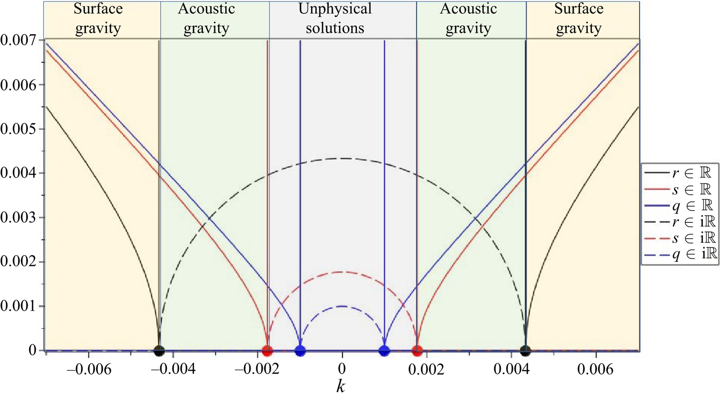
Figure 2 shows the various zones where  $r, q$ and $s$ take on real and imaginary values. There are zones corresponding to surface waves and acoustic–gravity waves. The remaining zones close to $k=0$ are not physical solutions, since imaginary values taken on by $q$ and/or $s$ would imply oscillations at infinite depth in the elastic medium. Moreover, $q$ and $s$ have to be real and non-negative, otherwise oscillations would increase with increasing depth into the elastic medium. Examination of $I_{1}, I_{2}, I_{3}$ indicates that possible poles might also exist at $k=0$ and when $k^{2}+s^{2}=0$. When $k=0$ the $\sin (kb)$ term in the numerator (from $H_{1}$ and $H_{3}$) ensures a factor of $b$ is reached in the limit $k\rightarrow 0$, so $k=0$ is a removable singularity. For the case $k^{2}+s^{2}=0$ there is a possible pole when $k={\omega }/{\sqrt {2}C_{s}}$, but this pole lies in the unphysical zone of figure 2. From Eyov et al. (Reference Eyov, Klar, Kadri and Stiassnie2013) we have that $s=0$ (at $k_{s}$) represents a point where the energy spreads out over the whole solid depth. At that point the wave amplitude vanishes and so propagation ceases.
Zones possible according to  $r, q, s$ being real or imaginary for the case $\omega = 2{\rm \pi}, C_{l}=1450\ {\rm m s}^{-1}, C_{s}=3550\ {\rm m s}^{-1}, C_{p}=6300\ {\rm m s}^{-1}$. Zone 1 (orange) has $r,q,s\in \mathbb {R}$ and corresponds to surface–gravity waves. Zone 2 (green) has $r \in \textrm {i}\mathbb {R}, {\rm with}\ q, s \in \mathbb {R}$ and corresponds to acoustic–gravity waves. The remaining zones near $k=0$ (grey) are not physical solutions. The points where $r,s,q$ transition real $\rightleftharpoons$ imaginary are designated $\pm k_{r}=\pm 0.00433$ (black circles), $\pm k_{s}=\pm 0.00177$ (red circles) and $\pm k_{q}=\pm 0.00099$ (blue circles) respectively.
When  $r\Rightarrow r_{0m}$ with $m=0,1$,
 \begin{equation} r=\sqrt{k^{2}-{\omega^{2}}/{C_{l}^{2}}}, \quad \implies k_{0m}=\sqrt{\frac{\omega^{2}}{C_{l}^{2}}+r_{0m}^{2}}, \end{equation}
which corresponds to surface waves. There are two possible modes for surface waves. Mode 00 can propagate if  $\omega > \omega _{00}$ – the cut-off frequency for this mode. Mode 01 is the usual tsunami. If instead $r\Rightarrow \textrm {i} r_{n}$, then acoustic–gravity waves are possible, and
 \begin{equation} k_{n}=\sqrt{\frac{\omega^{2}}{C_{l}^{2}}-r_{n}^{2}}, \end{equation}
up to a maximum value of  $n=N$, after which the evanescent waves exist with wavenumber $\varLambda _{n}$:
 \begin{equation} k_{n}=\textrm{i}\varLambda_{n}=\textrm{i}\sqrt{r_{n}^{2}- \frac{\omega^{2}}{C_{l}^{2}}}=\sqrt{\frac{\omega^{2}}{C_{l}^{2}}-r_{n}^{2}}. \end{equation}
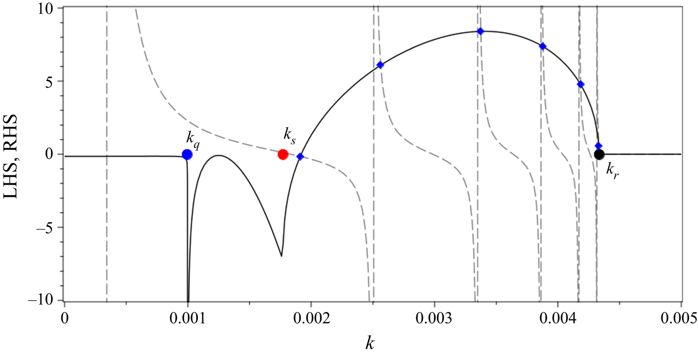
Solutions to the dispersion relation involving acoustic–gravity waves for the case  $\omega =2{\rm \pi}$ occur between $k_{s}=0.00177$ and $k_{r}=0.00433$. They are marked with blue diamonds in figure 3. Considering the liquid terms first, we break $\phi _{l0}$ into the different regions according to varying $\omega$. For $r\in \textrm {i}\mathbb {R}$:
 \begin{align} \phi_{l0}&=\frac{1}{2{\rm \pi}}\int_{-\infty}^{-\omega_{n}}\textrm{i}\,\textrm{d}\omega \, \textrm{e}^{-\textrm{i}\omega t}\frac{1}{2{\rm \pi} \textrm{i}}\int_{-\infty}^{\infty}\textrm{d} k\,\textrm{e}^{\textrm{i} kx}\frac{-H_{1}}{\omega kH_{2}}\left[\cos(\textrm{i} rz)-\frac{\textrm{i}\omega^{2}}{gr}\sin(\textrm{i} rz)\right] \nonumber\\ &\quad +\frac{1}{2{\rm \pi}}\int_{-\omega_{n}}^{\omega_{n}}\textrm{i}\,\textrm{d}\omega \, \textrm{e}^{-\textrm{i}\omega t}\frac{1}{2{\rm \pi} \textrm{i}}\int_{-\infty}^{\infty}\textrm{d} k\,\textrm{e}^{\textrm{i} kx}\frac{-H_{1}}{\omega kH_{2}}\left[\cos(\textrm{i} rz)-\frac{\textrm{i}\omega^{2}}{gr}\sin(\textrm{i} rz)\right]\nonumber\\ &\quad +\frac{1}{2{\rm \pi}}\int_{\omega_{n}}^{\infty}\textrm{i}\,\textrm{d}\omega \, \textrm{e}^{-\textrm{i}\omega t}\frac{1}{2{\rm \pi} \textrm{i}}\int_{-\infty}^{\infty}\textrm{d} k\,\textrm{e}^{\textrm{i} kx}\frac{-H_{1}}{\omega kH_{2}}\left[\cos(\textrm{i} rz)-\frac{\textrm{i}\omega^{2}}{gr}\sin(\textrm{i} rz)\right], \end{align}
whereas for  $r\in \mathbb {R}$:
 \begin{align} \phi_{l0}&=\frac{1}{2{\rm \pi}}\int_{-\infty}^{0}\textrm{i}\,\textrm{d}\omega \, \textrm{e}^{-\textrm{i}\omega t}\frac{1}{2{\rm \pi} \textrm{i}}\int_{-\infty}^{\infty}\textrm{d} k\,\textrm{e}^{\textrm{i} kx}\frac{-H_{1}}{\omega kH_{2}}\left[\cos(\textrm{i} rz)-\frac{\textrm{i}\omega^{2}}{gr}\sin(\textrm{i} rz)\right]\nonumber\\ &\quad +\frac{1}{2{\rm \pi}}\int_{0}^{\infty}\textrm{i}\,\textrm{d}\omega \, \textrm{e}^{-\textrm{i}\omega t}\frac{1}{2{\rm \pi} \textrm{i}}\int_{-\infty}^{\infty}\textrm{d} k\,\textrm{e}^{\textrm{i} kx}\frac{-H_{1}}{\omega kH_{2}}\left[\cos(\textrm{i} rz)- \frac{\textrm{i}\omega^{2}}{gr}\sin(\textrm{i} rz)\right]\nonumber\\ &\quad +\frac{1}{2{\rm \pi}}\int_{-\infty}^{-\omega_{00}}\textrm{i}\,\textrm{d}\omega \, \textrm{e}^{-\textrm{i}\omega t}\frac{1}{2{\rm \pi} \textrm{i}}\int_{-\infty}^{\infty}\textrm{d} k\,\textrm{e}^{\textrm{i} kx}\frac{-H_{1}}{\omega kH_{2}}\left[\cos(\textrm{i} rz)-\frac{\textrm{i}\omega^{2}}{gr}\sin(\textrm{i} rz)\right]\nonumber\\ &\quad +\frac{1}{2{\rm \pi}}\int_{\omega_{00}}^{\infty}\textrm{i}\,\textrm{d}\omega \, \textrm{e}^{-\textrm{i}\omega t}\frac{1}{2{\rm \pi} \textrm{i}}\int_{-\infty}^{\infty}\textrm{d} k\,\textrm{e}^{\textrm{i} kx}\frac{-H_{1}}{\omega kH_{2}}\left[\cos(\textrm{i} rz)-\frac{\textrm{i}\omega^{2}}{gr}\sin(\textrm{i} rz)\right]. \end{align}
Application of the Rayleigh damping method and contour integration using the residue theorem around a positively oriented simple closed curve as per Mei & Kadri (Reference Mei and Kadri2018) results in
 \begin{align} \phi_{l0}&=\frac{1}{2{\rm \pi}}\int_{-\infty}^{-\omega_{n}}\textrm{i}\,\textrm{d}\omega \, \textrm{e}^{-\textrm{i}\omega t}\sum_{n=1}^{N}\frac{-H_{1}|_{k={-}k_{n}}}{-\omega k_{n}\partial_{k}H_{2}|_{k={-}k_{n}}}\left[\cos(\textrm{i} rz)-\frac{\textrm{i}\omega^{2}}{gr}\sin(\textrm{i} rz)\right]\textrm{e}^{-\textrm{i} k_{n}x}\nonumber\\ &\quad +\frac{1}{2{\rm \pi}}\int_{-\omega_{n}}^{\omega_{n}}\textrm{i}\,\textrm{d}\omega \, \textrm{e}^{-\textrm{i}\omega t}\sum_{n=N+1}^{\infty}\frac{-H_{1}|_{k=\textrm{i}\varLambda_{n}}}{\omega \textrm{i}\varLambda_{n}\partial_{k}H_{2}|_{k=\textrm{i}\varLambda_{n}}}\left[\cos(\textrm{i} rz)-\frac{\textrm{i}\omega^{2}}{gr}\sin(\textrm{i} rz)\right]\textrm{e}^{-\varLambda_{n}x}\nonumber\\ &\quad +\frac{1}{2{\rm \pi}}\int_{\omega_{n}}^{\infty}\textrm{i}\,\textrm{d}\omega \, \textrm{e}^{-\textrm{i}\omega t}\sum_{n=1}^{N}\frac{-H_{1}|_{k=k_{n}}}{\omega k_{n}\partial_{k}H_{2}|_{k=k_{n}}}\left[\cos(\textrm{i} rz)-\frac{\textrm{i}\omega^{2}}{gr}\sin(\textrm{i} rz)\right]\textrm{e}^{\textrm{i} k_{n}x}, \end{align}
with  $r=\textrm {i} r_{n}\in \textrm {i}\mathbb {R}$, $\partial _{k}={\partial }/{\partial k}$,
 \begin{gather} H_{1}|_{k=k_{n}}=4\textrm{i} gr_{n}W_{0}\sin(k_{n}b)\sin(\omega T)\,\textrm{e}^{{-}q_{n}h}\left[{-}2k_{n}^{2}\mu q_{n}s_{n}\vphantom{\frac{\lambda}{2}}\right.\nonumber\\ \quad\qquad \ \ \left.+\,(k_{n}^{2}+s_{n}^{2})\left[\left(\mu+ \frac{\lambda}{2}\right)q_{n}^{2}-\frac{\lambda k_{n}^{2}}{2}\right]\right], \end{gather}
 \begin{gather} H_{1}|_{k={-}k_{n}}={-}H_{1}|_{k=k_{n}}, \end{gather}
 \begin{gather} H_{1}|_{k=\textrm{i}\varLambda_{n}}=4\textrm{i} g r_{n}W_{0}\sin(\textrm{i}\varLambda_{n}b)\sin(\omega T)\,\textrm{e}^{{-}q_{n}h}\left[2\varLambda_{n}^{2}\mu q_{n}s_{n}\vphantom{\frac{\lambda}{2}}\right.\nonumber\\ \qquad\qquad\ \left.+\,(s_{n}^{2}-\varLambda_{n}^{2}) \left[\left(\mu+\frac{\lambda}{2}\right)q_{n}^{2}+ \frac{\lambda\varLambda_{n}^{2}}{2}\right]\right]. \end{gather}
The derivative terms are given in Appendix A.
Acoustic–gravity wave solutions to the dispersion relation are located at the intersections of dashed and solid curves (blue diamonds) for  $\omega =2{\rm \pi}$ and depth $h=4000$ m. Dashed curve is left-hand side (LHS) of (3.44) and solid curve is right-hand side (RHS) of (3.44) when $r\in \textrm {i}\mathbb {R}$.
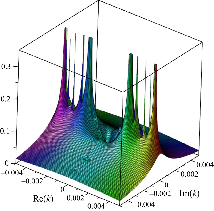
In support of the validity of the integration process figure 4 shows a plot of  ${1}/{|H_{2}|}$ in the complex plane when $H_{2}=H_{2}(k)$ and $k$ is allowed to take on complex values. Cross-sections through the real and imaginary axes appear in figures 5(a) and 5(b) respectively. The poles of the function lie on the real axis, whereas the zeros lie on the imaginary axis. If the range of the plots were to be extended then the function decays to zero everywhere. As empirical evidence for the validity of the integration, when the calculations are complete, we find good agreement with existing synthetic and real data plots for both acoustic–gravity waves and surface waves (e.g. see figures 13 and 17).
Plot of  ${1}/{|H_{2}|}$ in the complex plane when $H_{2}=H_{2}(k)$ and $k$ is allowed to take on complex values. The angular frequency in this case is $\omega =2{\rm \pi}$ as in figure 3.


In the case where  $r\Rightarrow r_{0m}, k\Rightarrow k_{0m}$ with $r_{0m}$ a real number and $m=0,1$ then there may exist two possibilities for surface waves:
 \begin{align}
\phi_{l0}&=\frac{1}{2{\rm \pi}}\int_{-\infty}^{0}\textrm{i}\,\textrm{d}\omega
\, \textrm{e}^{-\textrm{i}\omega
t}\frac{-H_{1}|_{k={-}k_{01}}}{-\omega
k_{01}\partial_{k}H_{2}|_{k={-}k_{01}}}\left[\cos(\textrm{i}
rz)-\frac{\textrm{i}\omega^{2}}{gr_{01}}\sin(\textrm{i}
rz)\right]\textrm{e}^{-\textrm{i} k_{01}x} \nonumber\\ &\quad
+\frac{1}{2{\rm \pi}}\int_{0}^{\infty}\textrm{i}\,\textrm{d}\omega
\, \textrm{e}^{-\textrm{i}\omega
t}\frac{-H_{1}|_{k=k_{01}}}{\omega
k_{01}\partial_{k}H_{2}|_{k=k_{01}}}\left[\cos(\textrm{i}
rz)-\frac{\textrm{i}\omega^{2}}{gr_{01}}\sin(\textrm{i}
rz)\right]\textrm{e}^{\textrm{i} k_{01}x}\nonumber\\ &\quad
+\frac{1}{2{\rm \pi}}\int_{-\infty}^{-\omega_{00}}\textrm{i}\,\textrm{d}\omega
\, \textrm{e}^{-\textrm{i}\omega
t}\frac{-H_{1}|_{k={-}k_{00}}}{-\omega
k_{00}\partial_{k}H_{2}|_{k={-}k_{00}}}\left[\cos(\textrm{i}
rz)-\frac{\textrm{i}\omega^{2}}{gr_{00}}\sin(\textrm{i}
rz)\right]\textrm{e}^{-\textrm{i} k_{00}x}\nonumber\\ &\quad
+\frac{1}{2{\rm \pi}}\int_{\omega_{00}}^{\infty}\textrm{i}\,\textrm{d}\omega
\, \textrm{e}^{-\textrm{i}\omega
t}\frac{-H_{1}|_{k=k_{00}}}{\omega
k_{00}\partial_{k}H_{2}|_{k=k_{00}}}\left[\cos(\textrm{i}
rz)-\frac{\textrm{i}\omega^{2}}{gr_{00}}\sin(\textrm{i}
rz)\right]\textrm{e}^{\textrm{i} k_{00}x},
\end{align}
\begin{align}
\phi_{l0}&=\frac{1}{2{\rm \pi}}\int_{-\infty}^{0}\textrm{i}\,\textrm{d}\omega
\, \textrm{e}^{-\textrm{i}\omega
t}\frac{-H_{1}|_{k={-}k_{01}}}{-\omega
k_{01}\partial_{k}H_{2}|_{k={-}k_{01}}}\left[\cos(\textrm{i}
rz)-\frac{\textrm{i}\omega^{2}}{gr_{01}}\sin(\textrm{i}
rz)\right]\textrm{e}^{-\textrm{i} k_{01}x} \nonumber\\ &\quad
+\frac{1}{2{\rm \pi}}\int_{0}^{\infty}\textrm{i}\,\textrm{d}\omega
\, \textrm{e}^{-\textrm{i}\omega
t}\frac{-H_{1}|_{k=k_{01}}}{\omega
k_{01}\partial_{k}H_{2}|_{k=k_{01}}}\left[\cos(\textrm{i}
rz)-\frac{\textrm{i}\omega^{2}}{gr_{01}}\sin(\textrm{i}
rz)\right]\textrm{e}^{\textrm{i} k_{01}x}\nonumber\\ &\quad
+\frac{1}{2{\rm \pi}}\int_{-\infty}^{-\omega_{00}}\textrm{i}\,\textrm{d}\omega
\, \textrm{e}^{-\textrm{i}\omega
t}\frac{-H_{1}|_{k={-}k_{00}}}{-\omega
k_{00}\partial_{k}H_{2}|_{k={-}k_{00}}}\left[\cos(\textrm{i}
rz)-\frac{\textrm{i}\omega^{2}}{gr_{00}}\sin(\textrm{i}
rz)\right]\textrm{e}^{-\textrm{i} k_{00}x}\nonumber\\ &\quad
+\frac{1}{2{\rm \pi}}\int_{\omega_{00}}^{\infty}\textrm{i}\,\textrm{d}\omega
\, \textrm{e}^{-\textrm{i}\omega
t}\frac{-H_{1}|_{k=k_{00}}}{\omega
k_{00}\partial_{k}H_{2}|_{k=k_{00}}}\left[\cos(\textrm{i}
rz)-\frac{\textrm{i}\omega^{2}}{gr_{00}}\sin(\textrm{i}
rz)\right]\textrm{e}^{\textrm{i} k_{00}x},
\end{align}
with
 \begin{align} H_{1}|_{k=k_{0m}}&=4gr_{0m}W_{0}\sin(k_{0m}b)\sin(\omega T)\,\textrm{e}^{{-}q_{0m}h}\left(\vphantom{\left.+(k_{0m}^{2}+s_{0m}^{2})\left(q_{0m}^{2} \left(\mu+\frac{\lambda}{2}\right)-\frac{\lambda k_{0m}^{2}}{2}\right)\right)}{-}2k_{0m}^{2}\mu q_{0m}s_{0m}\right.\nonumber\\ &\quad \left.+\,(k_{0m}^{2}+s_{0m}^{2})\left(q_{0m}^{2} \left(\mu+\frac{\lambda}{2}\right)-\frac{\lambda k_{0m}^{2}}{2}\right)\right), \end{align}
 \begin{equation} H_{1}|_{k={-}k_{0m}}={-}H_{1}|_{k=k_{0m}}. \end{equation}
The derivative term is again to be found in Appendix A. Using the substitutions
 \begin{equation} k=\sqrt{r^2+\frac{\omega^2}{C_{l}^2}},\quad q=\sqrt{r^2+\frac{\omega^2}{C_{l}^2} - \frac{\omega^2}{C_{p}^2}},\quad s=\sqrt{r^2+\frac{\omega^2}{C_{l}^2} - \frac{\omega^2}{C_{s}^2}}, \end{equation}
the dispersion relation (3.44) can be written in terms of  $r$ and $\omega$ alone, and in this case the condition for the existence of the $00$th mode for a particular $\omega$ is
 \begin{equation}
\frac{\textrm{d}}{\textrm{d} r} \bigl[{\rm left-hand
side of } (3.44)\bigr] >
\frac{\textrm{d}}{\textrm{d} r}
\bigl[{\rm right-hand side of } (3.44)\bigr]. \end{equation}
\begin{equation}
\frac{\textrm{d}}{\textrm{d} r} \bigl[{\rm left-hand
side of } (3.44)\bigr] >
\frac{\textrm{d}}{\textrm{d} r}
\bigl[{\rm right-hand side of } (3.44)\bigr]. \end{equation}
The expressions for the velocity potential in the liquid layer can be further reduced to
 \begin{align} \phi_{l0}&=\frac{1}{\rm \pi}\int_{\omega_{n}}^{\infty}\textrm{i}\,\textrm{d}\omega \, \textrm{e}^{-\textrm{i}\omega t}\sum_{n=1}^{N}\frac{-H_{1}|_{k=k_{n}}}{\omega k_{n}\partial_{k}H_{2}|_{k=k_{n}}}\left[\cos(\textrm{i} rz)-\frac{\textrm{i}\omega^{2}}{gr}\sin(\textrm{i} rz)\right]\textrm{e}^{\textrm{i} k_{n}x}\nonumber\\ &\quad +\frac{1}{\rm \pi}\int_{0}^{\infty}\textrm{i}\,\textrm{d}\omega \, \textrm{e}^{-\textrm{i}\omega t}\frac{-H_{1}|_{k=k_{01}}}{\omega k_{01}\partial_{k}H_{2}|_{k=k_{01}}}\left[\cos(\textrm{i} rz)-\frac{\textrm{i}\omega^{2}}{gr}\sin(\textrm{i} rz)\right]\textrm{e}^{\textrm{i} k_{01}x}\nonumber\\ &\quad +\frac{1}{\rm \pi}\int_{\omega_{00}}^{\infty}\textrm{i}\,\textrm{d}\omega \, \textrm{e}^{-\textrm{i}\omega t}\frac{-H_{1}|_{k=k_{00}}}{\omega k_{00}\partial_{k}H_{2}|_{k=k_{00}}}\left[\cos(\textrm{i} rz)-\frac{\textrm{i}\omega^{2}}{gr}\sin(\textrm{i} rz)\right]\textrm{e}^{\textrm{i} k_{00}x}\nonumber\\ &\quad +\frac{1}{\rm \pi}\int_{0}^{\omega_{n}}\textrm{i}\,\textrm{d}\omega \, \textrm{e}^{-\textrm{i}\omega t}\sum_{n=n+1}^{\infty}\frac{-H_{1}|_{k=\textrm{i}\varLambda_{n}}}{\omega \textrm{i}\varLambda_{n}\partial_{k}H_{2}|_{k=\textrm{i}\varLambda_{n}}}\left[\cos(\textrm{i} rz)-\frac{\textrm{i}\omega^{2}}{gr}\sin(\textrm{i} rz)\right]\textrm{e}^{-\varLambda_{n}x}. \end{align}
Returning to the expression for the displacement potential in the solid given by
 \begin{equation} \phi_{s0}=\frac{1}{2{\rm \pi}}\int_{-\infty}^{\infty}\textrm{i}\,\textrm{d}\omega \, \textrm{e}^{-\textrm{i}\omega t}\frac{1}{2{\rm \pi} \textrm{i}}\int_{-\infty}^{\infty}\textrm{d} k\,\textrm{e}^{\textrm{i} kx}\frac{H_{3}}{kH_{2}}\,\textrm{e}^{qz}, \end{equation}
and following a similar procedure to that of the liquid velocity potential case, we arrive at
 \begin{align} \phi_{s0}& =\frac{1}{\rm \pi}\int_{\omega_{n}}^{\infty}\textrm{i}\,\textrm{d}\omega\textrm{e}^{-\textrm{i}\omega t}\sum_{n=1}^{N}\frac{H_{3}|_{k=k_{n}}}{k_{n}\partial_{k}H_{2}|_{k=k_{n}}}\, \textrm{e}^{q_{n}z}\, \textrm{e}^{\textrm{i} k_{n}x}\nonumber\\ &\quad +\frac{1}{\rm \pi}\int_{0}^{\infty}\textrm{i}\,\textrm{d}\omega \, \textrm{e}^{-\textrm{i}\omega t}\frac{H_{3}|_{k=k_{01}}}{k_{01}\partial_{k}H_{2}|_{k=k_{01}}}\, \textrm{e}^{q_{01}z}\, \textrm{e}^{\textrm{i} k_{01}x}\nonumber\\ &\quad +\frac{1}{\rm \pi}\int_{\omega_{00}}^{\infty}\textrm{i}\,\textrm{d}\omega \, \textrm{e}^{-\textrm{i}\omega t}\frac{H_{3}|_{k=k_{00}}}{k_{00}\partial_{k}H_{2}|_{k=k_{00}}}\, \textrm{e}^{q_{00}z}\, \textrm{e}^{\textrm{i} k_{00}x}\nonumber\\ &\quad +\frac{1}{\rm \pi}\int_{0}^{\omega_{n}}\textrm{i}\,\textrm{d}\omega \, \textrm{e}^{-\textrm{i}\omega t}\sum_{n=N+1}^{\infty}\frac{H_{3}|_{k=\textrm{i}\varLambda_{n}}}{\textrm{i}\varLambda_{n}\partial_{k}H_{2}|_{k=\textrm{i}\varLambda_{n}}}\, \textrm{e}^{q_{n}z-\varLambda_{n}x}, \end{align}
with
 \begin{equation} \left.\begin{array}{c@{}}
H_{3}|_{k=k_{n}}={-}2 \rho_{l}W_{0}(k_{n}^{2}+s_{n}^{2})
\sin(k_{n}b)\sin(\omega
T)(\omega^{2}\sin(r_{n}h)-gr_{n}\cos(r_{n}h)),\\
H_{3}|_{k=k_{0m}}=2i\rho_{l}W_{0}(k_{0m}^{2}+s_{0m}^{2})
\sin(k_{0m}b)\sin(\omega
T)(\omega^{2}\sinh(r_{0m}h)-gr_{0m}\cosh(r_{0m}h)),\\
H_{3}|_{k=\textrm{i}\varLambda_{n}}=2\textrm{i}\rho_{l}W_{0}
(s_{n}^{2}-\varLambda_{n}^{2})\sinh
(\varLambda_{n}b)\sin(\omega
T)(\omega^{2}\sin(r_{n}h)-gr_{n}\cos(r_{n}h)).
\end{array}\right\} \end{equation}
\begin{equation} \left.\begin{array}{c@{}}
H_{3}|_{k=k_{n}}={-}2 \rho_{l}W_{0}(k_{n}^{2}+s_{n}^{2})
\sin(k_{n}b)\sin(\omega
T)(\omega^{2}\sin(r_{n}h)-gr_{n}\cos(r_{n}h)),\\
H_{3}|_{k=k_{0m}}=2i\rho_{l}W_{0}(k_{0m}^{2}+s_{0m}^{2})
\sin(k_{0m}b)\sin(\omega
T)(\omega^{2}\sinh(r_{0m}h)-gr_{0m}\cosh(r_{0m}h)),\\
H_{3}|_{k=\textrm{i}\varLambda_{n}}=2\textrm{i}\rho_{l}W_{0}
(s_{n}^{2}-\varLambda_{n}^{2})\sinh
(\varLambda_{n}b)\sin(\omega
T)(\omega^{2}\sin(r_{n}h)-gr_{n}\cos(r_{n}h)).
\end{array}\right\} \end{equation}
The derivative terms evaluated at  $k= k_{n}$, $k=\textrm {i}\varLambda _{n}$ and $k=k_{0m}$ remain as before. In a similar way the rotation potential can be written as
 \begin{equation} \psi_{0y}=\frac{1}{2{\rm \pi}}\int_{-\infty}^{\infty}\textrm{i}\,\textrm{d}\omega\,\textrm{e}^{-\textrm{i}\omega t}\frac{1}{2{\rm \pi} \textrm{i}}\int_{-\infty}^{\infty}\textrm{d} k\,\textrm{e}^{\textrm{i} kx}\frac{2\,\textrm{i} q}{k^{2}+s^{2}}\frac{H_{3}}{H_{2}}\,\textrm{e}^{h(s-q)+sz}, \end{equation}
which becomes
 \begin{align} \psi_{0y}& =\frac{1}{\rm \pi}\int_{\omega_{n}}^{\infty}\textrm{i}\,\textrm{d}\omega \, \textrm{e}^{-\textrm{i}\omega t}\sum_{n=1}^{N}\frac{2\,\textrm{i} q_{n}}{k_{n}^{2}+s_{n}^{2}}\frac{H_{3}|_{k=k_{n}}}{\partial_{k}H_{2}|_{k=k_{n}}}\, \textrm{e}^{h(s_{n}-q_{n})+s_{n}z}\, \textrm{e}^{\textrm{i} k_{n}x}\nonumber\\ & \quad +\frac{1}{\rm \pi}\int_{0}^{\infty}\textrm{i}\,\textrm{d}\omega \, \textrm{e}^{-\textrm{i}\omega t}\frac{2\,\textrm{i} q_{01}}{k_{01}^{2}+s_{01}^{2}}\frac{H_{3}|_{k=k_{01}}}{\partial_{k}H_{2}|_{k=k_{01}}}\, \textrm{e}^{h(s_{01}-q_{01})+s_{01}z}\, \textrm{e}^{\textrm{i} k_{01}x}\nonumber\\ & \quad +\frac{1}{\rm \pi}\int_{\omega_{00}}^{\infty}\textrm{i}\,\textrm{d}\omega \, \textrm{e}^{-\textrm{i}\omega t}\frac{2\,\textrm{i} q_{00}}{k_{00}^{2}+s_{00}^{2}}\frac{H_{3}|_{k=k_{00}}}{\partial_{k}H_{2}|_{k=k_{00}}}\, \textrm{e}^{h(s_{00}-q_{00})+s_{00}z}\, \textrm{e}^{\textrm{i} k_{00}x}\nonumber\\ & \quad +\frac{1}{\rm \pi}\int_{0}^{\omega_{n}}\textrm{i}\,\textrm{d}\omega \, \textrm{e}^{-\textrm{i}\omega t}\sum_{n=N+1}^{\infty}\frac{2\,\textrm{i} q_{n}}{s_{n}^{2}-\varLambda_{n}^{2}}\frac{H_{3}|_{k=\textrm{i}\varLambda_{n}}}{\partial_{k}H_{2}|_{k=\textrm{i}\varLambda_{n}}}\, \textrm{e}^{h(s_{n}-q_{n})+s_{n}z-\varLambda_{n}x}. \end{align}
3.5. Long-range modulation: liquid layer
We introduce unknown envelope factors for the liquid layer  $A_{n}^{\pm }(X,Y)$ and $A_{0m}^{\pm }(X,Y)$:
 \begin{align} \phi_{l0}&=\frac{1}{2{\rm \pi}}\int_{\omega_{n}}^{\infty}\textrm{i}\,\textrm{d}\omega \, \textrm{e}^{-\textrm{i}\omega t}\sum_{n=1}^{N}A_{n}^+\frac{-H_{1}|_{k=k_{n}}}{\omega k_{n}\partial_{k}H_{2}|_{k=k_{n}}}\left[\cos(\textrm{i} rz)-\frac{\textrm{i}\omega^{2}}{gr_{n}}\sin(\textrm{i} rz)\right]\textrm{e}^{\textrm{i} k_{n}x}\nonumber\\ &\quad +\frac{1}{2{\rm \pi}}\int_{0}^{\infty}\textrm{i}\,\textrm{d}\omega \, \textrm{e}^{-\textrm{i}\omega t}A_{01}^+\frac{-H_{1}|_{k=k_{01}}}{\omega k_{01}\partial_{k}H_{2}|_{k=k_{01}}}\left[\cos(\textrm{i} rz)-\frac{\textrm{i}\omega^{2}}{gr}\sin(\textrm{i} rz)\right]\textrm{e}^{\textrm{i} k_{01}x}\nonumber\\ &\quad +\frac{1}{2{\rm \pi}}\int_{\omega_{00}}^{\infty}\textrm{i}\,\textrm{d}\omega \, \textrm{e}^{-\textrm{i}\omega t}A_{00}^+\frac{-H_{1}|_{k=k_{00}}}{\omega k_{00}\partial_{k}H_{2}|_{k=k_{00}}}\left[\cos(\textrm{i} rz)-\frac{\textrm{i}\omega^{2}}{gr}\sin(\textrm{i} rz)\right]\textrm{e}^{\textrm{i} k_{00}x}\nonumber\\ &\quad +\frac{1}{2{\rm \pi}}\int_{-\infty}^{-\omega_{n}}\textrm{i}\,\textrm{d}\omega \, \textrm{e}^{-\textrm{i}\omega t}\sum_{n=1}^{N}A_{n}^{-}\frac{-H_{1}|_{k={-}k_{n}}}{-\omega k_{n}\partial_{k}H_{2}|_{k={-}k_{n}}}\left[\cos(\textrm{i} rz)-\frac{\textrm{i}\omega^{2}}{gr}\sin(\textrm{i} rz)\right]\textrm{e}^{-\textrm{i} k_{n}x}\nonumber\\ &\quad +\frac{1}{2{\rm \pi}}\int_{-\infty}^{0}\textrm{i}\,\textrm{d}\omega \, \textrm{e}^{-\textrm{i}\omega t}A_{01}^{-}\frac{-H_{1}|_{k={-}k_{01}}}{-\omega k_{01}\partial_{k}H_{2}|_{k={-}k_{01}}}\left[\cos(\textrm{i} rz)-\frac{\textrm{i}\omega^{2}}{gr}\sin(\textrm{i} rz)\right]\textrm{e}^{-\textrm{i} k_{01}x}\nonumber\\ &\quad +\frac{1}{2{\rm \pi}}\int_{-\infty}^{-\omega_{00}}\textrm{i}\,\textrm{d}\omega \, \textrm{e}^{-\textrm{i}\omega t}A_{00}^{-}\frac{-H_{1}|_{k={-}k_{00}}}{-\omega k_{00}\partial_{k}H_{2}|_{k={-}k_{00}}}\left[\cos(\textrm{i} rz)-\frac{\textrm{i}\omega^{2}}{gr}\sin(\textrm{i} rz)\right]\textrm{e}^{-\textrm{i} k_{00}x}\nonumber\\ &\quad +\frac{1}{2{\rm \pi}}\left[\int_{-\omega_{n}}^{0}+\int_{0}^{\omega_{n}}\right]\textrm{i}\,\textrm{d}\omega \, \textrm{e}^{-\textrm{i}\omega t}\sum_{n=N+1}^{\infty}\frac{-H_{1}|_{k=\textrm{i}\varLambda_{n}}}{\omega \textrm{i}\varLambda_{n}\partial_{k}H_{2}|_{k=\textrm{i}\varLambda_{n}}}\left[\cos(\textrm{i} rz)-\frac{\textrm{i}\omega^{2}}{gr}\sin(\textrm{i} rz)\right]\textrm{e}^{-\varLambda_{n}x}. \end{align}
The initial conditions are given by
 \begin{equation} A_{n}^{{\pm}}=\begin{cases} 1 & |Y|< {\unicode{x00A3}}=\epsilon L\\ 0 & |Y|> {\unicode{x00A3}}=\epsilon L , \end{cases} \quad A_{0m}^{{\pm}}=\begin{cases} 1 & Y|< {\unicode{x00A3}}=\epsilon L\\ 0 & Y|> {\unicode{x00A3}}=\epsilon L , \end{cases} \quad X=\epsilon^{2}x\rightarrow 0. \end{equation}
The waves are required to vanish far away from, and be symmetric about, the central axis (Mei & Kadri Reference Mei and Kadri2018):
 \begin{equation} A_{n}^{{\pm}}=A_{0m}^{{\pm}}=0,\quad |Y|\rightarrow\infty,\quad \frac{\partial A_{n}^{{\pm}}}{\partial Y}=\frac{\partial A_{0m}^{{\pm}}}{\partial Y}=0,\quad Y=0. \end{equation}
Proceeding with acoustic modes, taking the time Fourier transform of (3.8) and separating  $\bar {\phi }_{l2}$ into three ranges yields
 \begin{equation}
\bar{\phi}_{l2}=\begin{cases} \bar{\phi}_{l2}^+ &
\omega_{n}<\omega<\infty\\ \bar{\phi}_{l2}^{e} &
-\omega_{n}<\omega<\omega_{n}\\ \bar{\phi}_{l2}^{-} &
-\infty<\omega<{-}\omega_{n} .
\end{cases} \end{equation}
\begin{equation}
\bar{\phi}_{l2}=\begin{cases} \bar{\phi}_{l2}^+ &
\omega_{n}<\omega<\infty\\ \bar{\phi}_{l2}^{e} &
-\omega_{n}<\omega<\omega_{n}\\ \bar{\phi}_{l2}^{-} &
-\infty<\omega<{-}\omega_{n} .
\end{cases} \end{equation}
In the range  $\omega _{n}<\omega <\infty$,
 \begin{equation} \frac{\partial^{2}\bar{\phi}_{l2}^+}{\partial x^{2}}+\frac{\partial^{2}\bar{\phi}_{l2}^+}{\partial z^{2}}+\frac{\omega^{2}}{C_{l}^{2}}\bar{\phi}_{l2}^+{=}-\frac{\partial^{2}\bar{\phi}_{l0}}{\partial Y^{2}}-2\frac{\partial^{2}\bar{\phi}_{l0}}{\partial x\partial X}. \end{equation}
From this point the solution proceeds in an analogous way to that derived by Mei & Kadri (Reference Mei and Kadri2018):
 \begin{align} &\frac{\partial^{2}\bar{\phi}_{l2}^+}{\partial x^{2}}+\frac{\partial^{2}\bar{\phi}_{l2}^+}{\partial z^{2}}+\frac{\omega^{2}}{C_{l}^{2}}\bar{\phi}_{l2}^+{=}-\textrm{i}\sum_{n=1}^{N}\left[\frac{\partial^{2}A_{n}^+}{\partial Y^{2}}+2\,\textrm{i} k_{n}\frac{\partial A_{n}^+}{\partial X}\right]\nonumber\\ &\quad \frac{-H_{1}|_{k=k_{n}}}{\omega k_{n}\partial_{k}H_{2}|_{k=k_{n}}}\left[\cos(\textrm{i} rz)-\frac{\textrm{i}\omega^{2}}{gr}\sin(\textrm{i} rz)\right]\textrm{e}^{\textrm{i} k_{n}x}. \end{align}
Assuming  $\bar {\phi }_{l2}^+$ has solutions in the form $\sum _{n=1}^{N}\xi _{n}^+(\omega,z)\,\textrm {e}^{\textrm {i} k_{n}x}$, then substituting into (3.78) gives
 \begin{align} &-\sum_{n=1}^{N}\xi_{n}^+k_{n}^{2}\, \textrm{e}^{\textrm{i} k_{n}x}+\sum_{n=1}^{N}\frac{\partial^{2}\xi_{n}^+}{\partial z^{2}}\, \textrm{e}^{\textrm{i} k_{n}x}+\frac{\omega^{2}}{C_{l}^{2}}\sum_{n=1}^{N}\xi_{n}^+\, \textrm{e}^{\textrm{i} k_{n}x}\nonumber\\ &\quad ={-}\textrm{i}\sum_{n=1}^{N}\left[\frac{\partial^{2}A_{n}^+}{\partial Y^{2}}+2\,\textrm{i} k_{n}\frac{\partial A_{n}^+}{\partial X}\right]\frac{-H_{1}|_{k=k_{n}}}{\omega k_{n}\partial_{k}H_{2}|_{k=k_{n}}}F_{n}(z)\,\textrm{e}^{\textrm{i} k_{n}x}. \end{align}
Equating coefficients gives
 \begin{equation} \frac{\partial^{2}\xi_{n}^+}{\partial z^{2}}+\left(\frac{\omega^2}{C_{l}^2}-k_{n}^2\right) \xi_{n}^+{=}-\textrm{i}\left[\frac{\partial^{2}A_{n}^+}{\partial Y^{2}}+2\,\textrm{i} k_{n}\frac{\partial A_{n}^+}{\partial X}\right]\frac{-H_{1}|_{k=k_{n}}}{\omega k_{n}\partial_{k}H_{2}|_{k=k_{n}}}F_{n}(z), \end{equation}
where
 \begin{equation}
r^2=k^2-\frac{\omega^2}{C_{l}^2} \begin{cases}
r=r_{0m},\quad
\dfrac{\omega^2}{C_{l}^2}-k_{0m}^2={-}r_{0m}^2,\quad\textrm{surface
waves},\\ r=\textrm{i} r_{n},\quad
\dfrac{\omega^2}{C_{l}^2}-k_{n}^2={+}r_{n}^2,\quad\textrm{acoustic--gravity waves},
\end{cases} \end{equation}
\begin{equation}
r^2=k^2-\frac{\omega^2}{C_{l}^2} \begin{cases}
r=r_{0m},\quad
\dfrac{\omega^2}{C_{l}^2}-k_{0m}^2={-}r_{0m}^2,\quad\textrm{surface
waves},\\ r=\textrm{i} r_{n},\quad
\dfrac{\omega^2}{C_{l}^2}-k_{n}^2={+}r_{n}^2,\quad\textrm{acoustic--gravity waves},
\end{cases} \end{equation}
resulting in
 \begin{equation} \frac{\partial^{2}\xi_{n}^+}{\partial z^{2}}+r_{n}^{2}\xi_{n}^+{=}-\textrm{i}\left[\frac{\partial^{2}A_{n}^+}{\partial Y^{2}}+2\,\textrm{i} k_{n}\frac{\partial A_{n}^+}{\partial X}\right]\frac{-H_{1}|_{k=k_{n}}}{\omega k_{n}\partial_{k}H_{2}|_{k=k_{n}}}F_{n}(z), \end{equation}
where
 \begin{equation} F_{n}(z)=\cos({r_{n}z})+\frac{\omega^2}{g r_{n}}\sin({r_{n}z}). \end{equation}
The ground motion is captured at  $O(\epsilon ^0$), so the boundary conditions on $\bar {\phi }_{l2}^+$ (and therefore $\xi _{n}^+$) at O( $\epsilon ^2$) are
 $$\begin{gather} -\omega^2\bar{\phi}_{l2}^+{+}g\frac{\partial \bar{\phi}_{l2}^+}{\partial z}=0,\quad z=0, \end{gather}$$
 $$\begin{gather}\frac{\partial\bar{\phi}_{l2}^+}{\partial z}=0,\quad z={-}h. \end{gather}$$
Here  $F_{n}(z)$ is a solution to the boundary value problem:
 $$\begin{gather} \frac{\partial^{2} F_{n}}{\partial z^{2}}+r_{n}^{2} F_{n} = 0, \end{gather}$$
 $$\begin{gather}F_{n} = 1,\quad \frac{\partial F_{n}}{\partial z}=\frac{\omega^2}{g},\quad z=0, \end{gather}$$
 $$\begin{gather}F_{n}=\cos({r_{n}h})-\frac{\omega^2}{g r_{n}}\sin({r_{n}h}),\quad\frac{\partial F_{n}}{\partial z} = r_{n} \sin(r_{n} h ) + \frac{\omega^2}{g}\cos({ r_{n} h}), \quad z={-}h. \end{gather}$$
A similar process could be carried out for surface waves.
The next step is to extract the Schrödinger equation from (3.82) by applying the following Green's identity over the range  $-h \leq z \leq 0$:
 \begin{align} \int_{{-}h}^{0}\left[F_{n}\left(\frac{\partial^{2}\xi_{n}^+}{\partial z^{2}}+r_{n}^{2}\xi_{n}^+\right)-\xi_{n}^+\left(\frac{\partial^{2}F_{n}}{\partial z^{2}}+r_{n}^{2}F_{n}\right)\right]\textrm{d} z=\left[F_{n}\frac{\partial\xi_{n}^+}{\partial z}-\xi_{n}^+\frac{\partial F_{n}}{\partial z}\right]_{{-}h}^{0}. \end{align}
As in Mei & Kadri (Reference Mei and Kadri2018), the result is the Schrödinger equation for the two-dimensional evolution of the envelope factors:
 \begin{equation} \frac{\partial^{2}A_{n}^+}{\partial Y^{2}}+2\,\textrm{i} k_{n}\frac{\partial A_{n}^+}{\partial X}=0,\quad r\in \textrm{i}\mathbb{R}. \end{equation}
Having obtained the Schrödinger equation (3.90) for the acoustic–gravity wave case in the liquid layer the solution is analogous to that found in Mei & Kadri (Reference Mei and Kadri2018), but with mode properties now incorporating elasticity, via  $k_{n}$. The envelope solution is therefore stated here as
 \begin{align} A_{n}&=\frac{1-{\rm i}}{2}\left\{ C\left(\sqrt{\frac{2}{{\rm \pi}\chi_{n}}}\mathcal{Y_+}\right)+ C\left(\sqrt{\frac{2}{{\rm \pi}\chi_{n}}}\mathcal{Y_{-}}\right)\right\}\nonumber\\ &\quad +\frac{1+{\rm i}}{2}\left\{ S\left(\sqrt{\frac{2}{{\rm \pi}\chi_{n}}}\mathcal{Y_+}\right)+S\left(\sqrt{\frac{2}{{\rm \pi}\chi_{n}}}\mathcal{Y_{-}}\right)\right\},\quad \chi_{n}=\frac{X}{2k_{n}},\quad \mathcal{Y}_{{\pm}}=\frac{{\unicode{x00A3}}\pm Y}{2}, \end{align}
where  $C(z)$ and $S(z)$ are Fresnel integrals. A similar process beginning at (3.76) can be applied to derive the expressions for the surface wave mode 01 and mode 00. Finally, the pressure obtained from the velocity potential (3.67) in the liquid (propagating parts) inclusive of envelope factors is given by
 \begin{align} P&=\frac{\rho_{l}}{\rm \pi}\int_{\omega_{n}}^{\infty}\,\textrm{d}\omega \sum_{n=1}^{N}\frac{-H_{1}|_{k=k_{n}} A_{n}}{k_{n}\partial_{k}H_{2}|_{k=k_{n}}}\left[\cos(rz) +\frac{\omega^{2}}{gr}\sin(rz)\right]\textrm{e}^{\textrm{i} (k_{n}x-\omega t)}\nonumber\\ &\quad +\frac{\rho_{l}}{\rm \pi}\int_{0}^{\infty}\,\textrm{d}\omega \frac{-H_{1}|_{k=k_{01}} A_{01}}{k_{01}\partial_{k}H_{2}|_{k=k_{01}}} \left[\cosh(rz)+\frac{\omega^{2}}{gr}\sinh( rz)\right]\textrm{e}^{\textrm{i}(k_{01}x-\omega t)}\nonumber\\ &\quad +\frac{\rho_{l}}{\rm \pi}\int_{\omega_{00}}^{\infty}\,\textrm{d}\omega \frac{-H_{1}|_{k=k_{00}} A_{00}}{k_{00}\partial_{k}H_{2}|_{k=k_{00}}} \left[\cosh(rz)+\frac{\omega^{2}}{gr}\sinh( rz)\right]\textrm{e}^{\textrm{i}(k_{00}x-\omega t)}. \end{align}
Similarly the surface elevation is given by
 \begin{align} \eta&=\frac{1}{g{\rm \pi}}\int_{\omega_{n}}^{\infty}\,\textrm{d}\omega \sum_{n=1}^{N}\frac{-H_{1}|_{k=k_{n}} A_{n}}{k_{n}\partial_{k}H_{2}|_{k=k_{n}}}\, \textrm{e}^{\textrm{i} (k_{n}x-\omega t)} +\frac{1}{g{\rm \pi}}\int_{0}^{\infty}\,\textrm{d}\omega \frac{-H_{1}|_{k=k_{01}} A_{01}}{k_{01}\partial_{k}H_{2}|_{k=k_{01}}}\, \textrm{e}^{\textrm{i}(k_{01}x-\omega t)}\nonumber\\ &\quad +\frac{1}{g{\rm \pi}}\int_{\omega_{00}}^{\infty}\,\textrm{d}\omega \frac{-H_{1}|_{k=k_{00}} A_{00}}{k_{00}\partial_{k}H_{2}|_{k=k_{00}}}\, \textrm{e}^{\textrm{i}(k_{00}x-\omega t)}. \end{align}
4. Improved critical frequency approximations
In a practical application of (3.92) and (3.93) numerical solutions approximate the integrals over a finite range, and so knowledge of the critical frequencies  $\omega _{n}$ and $\omega _{00}$ is essential. The critical frequencies $\omega _{n}$ represent the cut-off for acoustic–gravity wave mode numbers $n\geq 2$, and $\omega _{00}$ is the cut-off for the surface wave mode 00. The first acoustic–gravity wave mode does not have a cut-off frequency (see figure 6b). An approximation for $\omega _{n}$ exists in the form of (4.1) (Eyov et al. Reference Eyov, Klar, Kadri and Stiassnie2013), but this approximation is based upon the location of the vertical asymptotes found in the dispersion relation plots, an example of which is shown in figure 6(a). This approximation – although compact and easy to use – is not as accurate as it might be. The following subsections construct a more accurate approximation for $\omega _{n}$ (albeit more complicated) and an approximation to the cut-off frequency of surface wave mode 00 based on the gradient condition (3.66).
Approximate critical values from (4.1) (red circles) and actual critical values (blue circles). (a) Dispersion relation plot for  $h=4000$ m. Red circle marks vertical asymptote. Blue circle marks $r_{2}$, the actual cut-off for mode 2. Dashed trace, left-hand side (LHS) of equation (3.44); solid trace, right-hand side (RHS) of equation (3.44). (b) Phase velocity curves for first four modes at constant depth of $h=4000$ m. Dotted line is $C_{s}=3550\ \textrm {m s}^{-1}$.

4.1. Acoustic–gravity waves
When the acoustic–gravity wave propagating modes ( $n=2,3,\ldots$) terminate, the phase velocity becomes equal to $C_{s}$ and $s=\sqrt {k^2-{\omega ^2}/{C_{s}^2}}=0$ (Eyov et al. Reference Eyov, Klar, Kadri and Stiassnie2013). The first progressive mode ( $n=1$) for an elastic seabed is a Scholte wave, which propagates all the way to the shore, where it turns into a Rayleigh wave. From (30) of Eyov et al. (Reference Eyov, Klar, Kadri and Stiassnie2013), the critical frequency for a particular depth is given by
 \begin{equation} \omega_{en}=\left(n-\frac{3}{2}\right){\rm \pi} \frac{C_{l}C_{s}}{h_{en} \sqrt{C_{s}^2 - C_{l}^2}}\quad n=2,3,\ldots, \end{equation}
which is a good approximation to the actual critical frequency, though it is based on the location of the vertical asymptotes in the dispersion relation plot – location of red circle in figure 6(a). For accuracy, we require a better approximation to the actual intersection of the two curves in the dispersion relation plot – blue circle in figure 6(a). We begin with the dimensionless form of the dispersion relation (3.44):
 \begin{equation} \tanh(\tilde{r})=\frac{\dfrac{\tilde{\omega}^{2}}{\tilde{r}} (\varepsilon_{2}+\varepsilon_{1})}{\dfrac{\tilde{\omega}^{4}}{\tilde{r}^{2}} \varepsilon_{2}+\varepsilon_{1}},\quad \varepsilon_{1}=\frac{4\tilde{k}^{2}\tilde{q}\tilde{s} \tilde{\mu}}{\tilde{k}^{2}+\tilde{s}^{2}}+\tilde{\lambda} \tilde{k}^{2}-(\tilde{\lambda}+2\tilde{\mu})\tilde{q}^{2}, \quad \varepsilon_{2}=\tilde{q}\left(\frac{\tilde{k}^{2}- \tilde{s}^{2}}{\tilde{k}^{2}+\tilde{s}^{2}}\right), \end{equation}
with  $r, k, q, s, \omega, \lambda, \mu, C_{l}, C_{s}, C_{p}$ made dimensionless according to
 \begin{equation} \left.\begin{array}{c} \displaystyle \tilde{r}=hr, \quad \tilde{k}=hk, \quad \tilde{q}=hq, \quad \tilde{s}=hs, \quad \tilde{\omega}=\sqrt{\dfrac{h}{g}}\omega , \quad \tilde{\lambda}=\dfrac{\lambda}{\rho_{l} gh}, \quad \tilde{\mu}=\dfrac{\mu}{\rho_{l} gh}, \\ \displaystyle \widetilde{C_{l}}=\dfrac{C_{l}}{\sqrt{gh}}, \quad \widetilde{C_{s}}=\dfrac{C_{s}}{\sqrt{gh}}, \quad \widetilde{C_{p}}=\dfrac{C_{p}}{\sqrt{gh}}. \end{array}\right\} \end{equation}
We substitute
 \begin{equation}
\tilde{k}=\sqrt{\tilde{r}^{2}+\frac{\tilde{\omega}^{2}}{\widetilde{C_{l}}^{2}}},
\quad
\tilde{q}=\sqrt{\tilde{r}^{2}+\frac{\tilde{\omega}^{2}}{\widetilde{C_{l}}^{2}}-
\smash{\frac{\tilde{\omega}^{2}}{\widetilde{C_{p}}^{2}}}}, \quad
\tilde{s}=\sqrt{\tilde{r}^{2}+\frac{\tilde{\omega}^{2}}{\widetilde{C_{l}}^{2}}-
\frac{\tilde{\omega}^{2}}{\widetilde{C_{s}}^{2}}}
\end{equation}
\begin{equation}
\tilde{k}=\sqrt{\tilde{r}^{2}+\frac{\tilde{\omega}^{2}}{\widetilde{C_{l}}^{2}}},
\quad
\tilde{q}=\sqrt{\tilde{r}^{2}+\frac{\tilde{\omega}^{2}}{\widetilde{C_{l}}^{2}}-
\smash{\frac{\tilde{\omega}^{2}}{\widetilde{C_{p}}^{2}}}}, \quad
\tilde{s}=\sqrt{\tilde{r}^{2}+\frac{\tilde{\omega}^{2}}{\widetilde{C_{l}}^{2}}-
\frac{\tilde{\omega}^{2}}{\widetilde{C_{s}}^{2}}}
\end{equation}
into (4.2) to obtain a function of  $\tilde {r}$ alone, followed by another substitution $\tilde {r}\Rightarrow \textrm {i} \tilde {r}$ to retrieve the acoustic–gravity wave solutions.
Let  $\tilde {\omega }={\tilde {r} \widetilde {C_{s}} \widetilde {C_{l}}}/{\sqrt {\widetilde {C_{s}}^{2}-\widetilde {C_{l}}^{2}}}$, which is the $\tilde {s}=0$ condition for the termination of progressive modes, and then let $\tilde {r}=(n-\frac {3}{2}){\rm \pi} +\delta (n)$, where $\delta (n)$ represents a small (mode-dependent) positive offset away from the vertical asymptotes located at $\tilde {r}=(n-\frac {3}{2}){\rm \pi}$. So the desired $\delta (n)$ is the $\tilde {r}$ separation between the blue and red circles in figure 6(a). Ignoring terms of $O(\delta (n)^2)$ an approximation of the dispersion relation (see Appendix B) can be written as
 \begin{equation} -\cot(\delta(n))=\frac{a_{n}+b_{n}\delta(n)}{c_{n}+d_{n}\delta(n)}, \end{equation}
where the coefficients  $a_{n}, b_{n}, c_{n}, d_{n}$ are given in Appendix C. Then using the approximation $-\cot (\delta (n))\simeq -{1}/{\delta (n)}$ for small $\delta (n)$, (4.5) can be put into quadratic form:
 \begin{equation} b_{n}\delta(n)^{2}+(a_{n}+d_{n})\delta(n)+c_{n}=0. \end{equation}
This can be solved for  $\delta (n)$, and then the value of $\tilde {r}_{n}$ and the critical frequency $\omega _{n}$ can be obtained from
 \begin{equation} \tilde{r}_{n}=\left(n-\frac{3}{2}\right){\rm \pi}+\delta(n). \end{equation}
To determine how well  $\delta (n)$ predicts the offset a comparison was made between the approximate value of $\omega _{n}$ calculated using (4.7) and that found by using the dispersion relation
 \begin{equation} {\rm error [\%]}=\left|\frac{\omega_{n}({\rm approx})- \omega_{n}({\rm dispersion})}{\omega_{n}({\rm dispersion})} \times100\right|. \end{equation}
The comparison was carried out for depths ranging from 500 to 8000 m and all available modes. The maximum error occurred in the second mode at a depth of 8000 m, but was still less than 0.1 % (see figure 7). In § 5 the results for  $\tilde {r}_{n}$ and $\delta (n)$ are used to construct approximate phase velocity curves.
Percentage error for approximate critical frequencies  $\omega _{n}$ from (4.7). Depths range between 500 m (lower error bound) and 8000 m (upper error bound) – all available modes.

4.2. Surface wave
The surface gravity mode 00 does not exist for all frequencies in the elastic seabed case and never exists for a rigid seabed. The cut-off condition for mode 00 is given by (3.66) which can be solved numerically for a given depth. Alternatively a good approximation can be obtained by seeking the frequency at which the gradient of the left-hand side of the dimensionless dispersion relation in (4.2) is equal to the gradient of the right-hand side. This occurs for small (ultimately zero)  $\tilde {r}$. In this case we make the approximation $\tanh (\tilde {r})\simeq \tilde {r}$. Now we differentiate (4.2) with respect to $\tilde {r}$. Then we express the result as a series in $\tilde {r}^2$ to arrive at
 \begin{equation} 1=\frac{1}{\tilde{\omega}^2}+\frac{\mathcal{A}}{\tilde{\omega}} +O(\tilde{r}^2). \end{equation}
In the limit  $\tilde {r}\rightarrow 0$, (4.9) can be written as the quadratic $\tilde {\omega }^2 -\mathcal {A} \tilde {\omega } -1=0$, with
 \begin{align} \mathcal{A}=2\frac{\left[\left(\tilde{\mu}+\dfrac{\tilde{\lambda}}{2}\right) \tilde{C}_{l}^2-\tilde{\mu}\tilde{C}_{p}^2\right] (2\tilde{C}_{s}^2-\tilde{C}_{l}^2)\sqrt{\tilde{C}_{s}^2- \tilde{C}_{l}^2}+2\tilde{C}_{p}\tilde{C}_{s}\tilde{\mu} \sqrt{\tilde{C}_{p}^2-\tilde{C}_{l}^2} (\tilde{C}_{s}^2-\tilde{C}_{l}^2)}{\tilde{C}_{l}^3 \tilde{C}_{p} \sqrt{\tilde{C}_{p}^2-\tilde{C}_{l}^2} \sqrt{\tilde{C}_{s}^2-\tilde{C}_{l}^2}}. \end{align}
Taking the positive root of the quadratic gives the approximate cut-off frequency which we name  $\tilde {\varOmega }_{00}$. The dimensional form can be recovered from $\varOmega _{00}=\tilde {\varOmega }_{00}\sqrt {\vphantom{\frac{a}{a}}{g}/{h}}$. A workable approximation to the cut-off frequency can be obtained by taking $\mathcal {A}$. We call this approximation $\mathcal {A}_{00}$. Table 1 gives values for $\omega _{00}$ found using a numeric solver and compares with the approximations $\varOmega _{00}$ and $\mathcal {A}_{00}$ indicating errors for various depths. The error values were calculated from
 \begin{equation} {\rm error [\%]}=\left|\frac{\varOmega_{00}({\rm or } \mathcal{A}_{00})-\omega_{00}}{\omega_{00}}\times100\right|. \end{equation}
Comparison of cut-off frequencies obtained from numeric solver ( $\omega _{00}$) with approximations from quadratic solution ( $\varOmega _{00}$) and coarse approximation ( $\mathcal {A}_{00}$) for various depths $h$.
$h$.

5. Approximate phase velocity curves: shearing method
When plotting phase velocity curves it is typical to choose one or other of the following scenarios: either (i) fix constant frequency  $\omega$ and plot phase velocity versus depth $h$ as in Eyov et al. (Reference Eyov, Klar, Kadri and Stiassnie2013) (figure 2a) or (ii) fix a constant depth and plot phase velocity versus frequency (as in this paper). In either case for each data point on every curve the dispersion relation has to be solved numerically which can be time-consuming. Also, care has to be taken to ensure solutions are valid. Here we present an alternative method for quickly plotting an approximate version of the elastic seabed phase velocity curves. In the following, variables with a tilde are made dimensionless according to (4.3). The method is based around the $\tanh ^{-1}$ function which is manipulated in the following ways.
• Scale along the horizontal $\tilde {r}$ axis (the independent variable) so as to fit the range $(n-\frac {3}{2}){\rm \pi} \ldots (n-\frac {1}{2}){\rm \pi}$, with $n$ being the mode number:
(5.1)\begin{equation} -\tanh^{{-}1}\left[\frac{2}{\rm \pi}(\tilde{r}-(n-1) {\rm \pi})\right]. \end{equation}
$\tilde {r}$ axis (the independent variable) so as to fit the range $(n-\frac {3}{2}){\rm \pi} \ldots (n-\frac {1}{2}){\rm \pi}$, with $n$ being the mode number:
(5.1)\begin{equation} -\tanh^{{-}1}\left[\frac{2}{\rm \pi}(\tilde{r}-(n-1) {\rm \pi})\right]. \end{equation}• Shift up the vertical axis so that at centre range
$\tilde {r}=(n-1){\rm \pi}$ the value is $\alpha Cs$, i.e. the Rayleigh wave phase velocity where the first acoustic mode intersects the vertical axis (see figure 6b). The value of $\alpha =0.922231$ is taken from (5.22) of Eyov (Reference Eyov2013):
(5.2)\begin{equation} \alpha C_{s} -\tanh^{{-}1}\left[\frac{2}{\rm \pi}(\tilde{r}- (n-1){\rm \pi})\right]. \end{equation}• Next stretch the plot along the vertical axis by a factor
$\tilde {\kappa }(n)$ so that the curve meets the shear velocity $C_{s}$ at the critical value $\tilde {r}_{n}$ determined from (4.7):
(5.3)where\begin{equation} \alpha C_{s} -\tilde{\kappa}(n)\tanh^{{-}1} \left[\frac{2}{\rm \pi}(\tilde{r}-(n-1){\rm \pi})\right], \end{equation}(5.4)and\begin{equation} \tilde{\kappa}(n)=\frac{\tilde{C}_{s}(\alpha-1)}{\tanh^{{-}1} \left[\dfrac{2}{\rm \pi}\left(-\dfrac{\rm \pi}{2}+\delta(n) \right)\right]}\end{equation}$\delta (n)$ is the critical offset calculated via the procedure described in § 4.• Include a multiplicative factor
$\tilde {Y}(\tilde {r},n)$ to ensure that the curve has its region of rapid descent shifted away from the $(n-\frac {1}{2}){\rm \pi}$ asymptote to better align with the ‘reference’ phase velocity curves derived from the dispersion relation, and so help minimise errors. The function $\tilde {v}(\tilde {r},n)$ so obtained is the generating function from which all the phase velocity curves are derived:
(5.5)where\begin{equation} \tilde{v}(\tilde{r},n)= \alpha C_{s} -\tilde{Y}(\tilde{r},n)\tilde{\kappa}(n)\tanh^{{-}1} \left[\frac{2}{\rm \pi}(\tilde{r}-(n-1){\rm \pi})\right], \end{equation}(5.6)The resulting curve for the case\begin{equation} \tilde{Y}(\tilde{r},n)=\frac{\left(n-\dfrac{1}{2}\right){\rm \pi}-\tilde{r} }{\sqrt{\left[\left(n-\dfrac{1}{2}\right){\rm \pi}-\tilde{r}\right]^2 - \left(\dfrac{\rm \pi}{18}\right)^2}}. \end{equation}$n=1$ is shown in figure 8. Curves for higher modes are obtained by shifting the $n=1$ case by appropriate multiples of ${\rm \pi}$ along the positive $\tilde {r}$ axis. The variable $\tilde {r}$ ranges over the interval $\tilde {r}_{n}\leq \tilde {r}\leq (\tilde {r}_{*}-\varepsilon )$ with $0<\varepsilon \ll 1$, defined by $(n-\frac {3}{2}){\rm \pi} <\tilde {r}_{n}\leq \tilde {r}\leq (\tilde {r}_{*}-\varepsilon )<(n-\frac {1}{2}){\rm \pi}$ and $\tilde {r}_{*}$ is such that $\tilde {v}(\tilde {r}_{*},n)=\tilde {C}_{l}$. This represents the phase velocity asymptotically approaching $C_{l}$ with increasing frequency (all modes).• Take the generating function for each mode and translate, so that the known point
$(\tilde {\omega }_{n},\tilde {C}_{s}) \rightarrow (0,0)$. This is the black curve $\tilde {t}(\tilde {r},n)$ in figure 9:
(5.7)where\begin{align} \tilde{t}(\tilde{r},n)=\tilde{r}\frac{\tilde{C}_{s} \tilde{C}_{l}}{\sqrt{\tilde{C}_{s}^2-\tilde{C}_{l}^2}}+\textrm{i} \tilde{v} - \tilde{z}_{n}, \quad \tilde{z}_{n}=\tilde{r}_{n} \frac{\tilde{C}_{s}\tilde{C}_{l}}{\sqrt{\tilde{C}_{s}^2-\tilde{C}_{l}^2}}+\textrm{i} \tilde{C}_{s},\quad \tilde{r}_{n}=\left(n-\frac{3}{2}\right){\rm \pi} + \delta(n), \end{align}$\tilde {z}_{n}$ is a fixed complex number representing the known cut-off point $(\tilde {\omega }_{n},\tilde {C}_{s})$.• Apply the shearing function
$\tilde {S}(\tilde {a},n)$ to distort the black curve into the appropriate shape for the mode considered – the coloured curves $\tilde {z}_{t_{n}}$ in figure 9:
(5.8)$$\begin{gather} \tilde{z}_{t_{n}}=[{\mbox{Re}}(\tilde{t})-\tilde{S}\,{\mbox{Im}} ({\tilde{t}})]+\textrm{i}\,{\mbox{Im}}(\tilde{t}), \end{gather}$$(5.9)A plot of$$\begin{gather}\tilde{S}(\tilde{a},n)=\frac{1}{\tilde{a}} [\tilde{w}(\tilde{a},n)-\tilde{w}(0,n)]. \end{gather}$$$\tilde {S}(\tilde {a},n)$ is shown in figure 10(b). The function $\tilde {w}(\tilde {a},n)$ is derived from the phase velocity curves for the rigid seabed case (figure 10a) by inverting (5.10) to give $\tilde {\omega }$ in terms of rigid seabed phase velocity $\tilde {v}_{r}$:
(5.10)The expressions for\begin{equation} \tilde{v}_{r}=\frac{\tilde{\omega}}{\tilde{k}_{n}}, \quad \tilde{k}_{n}=\sqrt{\frac{\tilde{\omega}^2}{\tilde{C}_{l}^2} - \frac{\tilde{\omega}_{rn}^2}{\tilde{C}_{l}^2}}, \quad \tilde{\omega}_{rn}=\left(n-\frac{1}{2} \right) {\rm \pi}\tilde{C}_{l}. \end{equation}$\tilde {k}_{n}$ and $\tilde {\omega }_{rn}$ appearing in (5.10) are from (3.9) and (3.10) of Mei & Kadri (Reference Mei and Kadri2018) here made dimensionless. After performing the inversion
(5.11)make the change of variable\begin{equation} \tilde{\omega}=\frac{\tilde{v}_{r} \tilde{\omega}_{rn}}{\sqrt{\tilde{v}_{r}^2 - \tilde{C}_{l}^2}}=\frac{\tilde{v}_{r}}{\sqrt{\tilde{v}^2 - \tilde{C}_{l}^2}}\left(n-\frac{1}{2} \right){\rm \pi} \tilde{C}_{l}, \end{equation}$\tilde {v}_{r}=\tilde {C}_{s}-\tilde {a}$, and rename $\tilde {\omega }$ to $\tilde {w}$ to arrive at
(5.12)The function\begin{equation} \tilde{w}(\tilde{a},n)=\frac{\tilde{C}_{s}-\tilde{a}}{\sqrt{(\tilde{C}_{s} - \tilde{a} )^2 - \tilde{C}_{l}^2}} \left(n-\frac{1}{2}\right){\rm \pi}\tilde{C}_{l}. \end{equation}$\tilde {a}$ is a measure of the vertical drop from the constant line $\tilde {C}_{s}$ down to the phase velocity curves $\tilde {v}_{r}$ (see figure 10a). In order to apply $\tilde {S}(\tilde {a},n)$ to the generating function define $\tilde {a}=C_{s}-\tilde {v}(\tilde {r},n)$ so now $\tilde {a}$ represents the vertical drop from the constant line $\tilde {C}_{s}$ down to the phase velocity curves $\tilde {v}(\tilde {r},n)$ (see figure 8).• Add
$\tilde {z}_{n}$ to translate back:
(5.13)\begin{equation} \tilde{z}=\tilde{z}_{t_{n}}+\tilde{z}_{n}= [{\mbox{Re}}(\tilde{t})-\tilde{S}\,{\mbox{Im}}({\tilde{t}})]+ \textrm{i}{\mbox{Im}}(\tilde{t})+ \tilde{z}_{n}. \end{equation}• Finally re-scale to obtain the desired phase velocity curves – solid black trace in figure 11:
(5.14)\begin{equation} \omega+\textrm{i} v_{e}=\tilde{\omega}\sqrt{\frac{g}{h}}+\textrm{i} \tilde{v}_{e} \sqrt{g h}={\mbox{Re}}({\tilde{z}})\sqrt{\frac{g}{h}}+\textrm{i}\, {\mbox{Im}}{(\tilde{z})} \sqrt{g h}. \end{equation}Figure 8.Generating function
$\tilde {v}(\tilde {r},n)$ for first acoustic–gravity mode ($n=1$) with depth $h=2000$ m. Other modes are derived by shifting the horizontal axis through $(n-1){\rm \pi}$ and using the appropriate values for $\tilde {r}_{n}$ and $\tilde {r}_{*}$.Figure 9.The black trace
$\tilde {t}$ is sheared by the action of $\tilde {S}$ into each of the coloured curves for each mode. Depth in this case is 2000 m, first eight modes shown. Then the result is translated and scaled to give the final phase velocity curves.Figure 10.Rigid seabed phase velocity curves along with shearing function. (a) Rigid seabed phase velocity
$\tilde {V}_{r}$ versus $\tilde {\omega }$. Depth $h=2000$ m. First eight modes. (b) Plot of shear function $\tilde {S}$ versus $\tilde {a}$. Depth $h=2000$ m. First eight modes.Figure 11.Overlay of phase velocity curves for depth of
$h=4000$ m. Solid black lines are the approximate curves, dashed are those obtained from solving the dispersion relation.The solid black trace of figure 11 is a complex plot with real part representing the angular frequency
$\omega$ and imaginary part representing the elastic seabed phase velocity $v_{e}$. The dashed curves of figure 11 are those obtained by numerically solving the dispersion relation (3.44). To quantify the errors between the phase velocity obtained using the shearing method and that obtained by solving the dispersion relation, use
(5.15)The maximum error occurs for the first mode and errors decrease with increasing frequency and increasing mode number (figure 12). There is some freedom in the expression for\begin{equation} {\rm error [\%]}=\left|\frac{v_{e}({\rm shear})- v_{e}({\rm dispersion})}{v_{e}({\rm dispersion})} \times100\right|. \end{equation}$\tilde {Y}(\tilde {r},n)$ which could potentially reduce the errors a little by carefully replacing the ${{\rm \pi} }/{18}$ term with an alternative value derived from some error minimisation technique (e.g. minimax approximation (Powell Reference Powell1996)), which we did not pursue further here.


Percentage error for first 16 modes. Depth  $h=4000$ m.

6. Numerical results
6.1. Acoustic–gravity waves
Figure 13 compares the first acoustic mode for the elastic case (3.92) and rigid case ((3.22) of Williams et al. (Reference Williams, Kadri and Abdolali2021)). As in Eyov et al. (Reference Eyov, Klar, Kadri and Stiassnie2013) the values used for  $\rho _{l}, \rho _{s}, C_{l}, C_{s}$ and $C_{p}$ are average values taken from Dziewonshi & Anderson (Reference Dziewonshi and Anderson1981). One stark difference between the two cases is that the signal terminates after some time in the elastic case, whereas it continues indefinitely in the rigid case. Another difference is the presence of signal at times earlier than the main pulse in the elastic case, but no signal at all in the rigid stationary phase model. The phase velocity curves for the elastic case (figure 11) indicate that frequencies close to the critical frequency for each mode receive a boost in phase velocity enabling signals to propagate faster. For these frequencies speeds close to $C_{s}$ are achievable. The rigid seabed stationary phase model produces complex numbers for times earlier than ${x}/{C_{l}}$ due to a singularity induced by the stationary phase method (Stiassnie Reference Stiassnie2010). The pressure amplitudes are similar.
First acoustic mode (a) with elastic seabed and (b) with rigid seabed.

A sensitivity analysis was carried out looking at the effects of six parameters on the signal duration (see figure 14). Each parameter was varied individually away from its reference value (table 2) while holding all other parameters at reference. Then the percentage change in pulse duration was divided by the percentage change in the parameter to arrive at the sensitivity value. It was found that the rigidity of the seabed most affected the signal duration. Increasing the Lamé parameters increases  $C_{s}$ and $C_{p}$ in accordance with (2.7a,b); the ratio ${C_{p}}/{C_{s}}$ was kept constant. Another difference between the elastic seabed case and the rigid seabed case appears when a fast Fourier transform of the signals is examined. The elastic case shows a slight upward shift in the frequency peak (see figure 15). This is in contrast to the slight downward shift found when a viscous compressible sediment layer is overlying the seabed as in Abdolali, Kirby & Bellotti (Reference Abdolali, Kirby and Bellotti2015). Whilst investigating the synthetic acoustic–gravity waves, we found that band-pass filtering applied to the signal generated by combining the first 10 modes (figure 16a) revealed some interesting peaks located close to the expected arrival time for a phase velocity of $C_{l}$ (figure 16b). There are four peaks of particular interest labelled 1, 2, 3 and 4. The presence of the peaks is a consequence of the fault's geometry and motion, and is not related to the rigidity of the seabed, since the peaks are also present under rigid seabed conditions, and even when the signal considered was purely acoustic, as in Mei & Kadri (Reference Mei and Kadri2018). The time spacing between pairs of peaks responds to changes in either fault half-width $b$ or rupture duration $\tau =2T$ in a linear fashion, so that details of the fault's geometry and dynamics are encoded in the acoustic–gravity waves. Time $\Delta t_{1}$ between peak numbers 1 and 2 (or 3 and 4) is exactly the rupture duration, and $\Delta t_{2}$ between peaks 1 and 3 (or 2 and 4) is linearly related to the fault half-width through $\Delta t_{2}={2b}/{C_{l}}$. When the slender fault begins to move, peaks 1 and 3 are generated at the edges of the slender fault and begin to propagate. The time separation between these peaks is explained as the time required for a wave travelling at speed $C_{l}$ to cross a fault width of $2b$. At the end of the fault's motion, after $\tau$ seconds, the second pair of peaks (2 and 4) is generated and propagates away – also separated in time by $\Delta t_{2}$. The resultant waveform as would be seen in the far field is a collection of four peaks. The amplitude of the peaks depends linearly on the uplift velocity $W_{0}$. The timings between peaks agree well with the values given in table 2. Let subscripts $1,2,3$ and $4$ represent the peaks denoted by the numbers 1, 2, 3 and 4 respectively. Then, $\Delta t_{12}=10.97\ \textrm {s}$, $\Delta t_{34}=8.9\ \textrm {s}$, $\Delta t_{13}=57.67\ \textrm {s}$ and $\Delta t_{24}=55.46\ \textrm {s}$. The times $\Delta t_{12}$ and $\Delta t_{34}$ represent $\tau$, the uplift time, which (from table 2) is actually 10 s. The times $\Delta t_{13}$ and $\Delta t_{24}$ are the transit times for an acoustic signal to cross a fault width $2b$, which, again from table 2, is actually 55.17 s. The information that could be extracted from the timings embedded in the acoustic modes would be of interest to the inverse process that reconstructs fault parameters from received signals (Gomez & Kadri Reference Gomez and Kadri2021). In § 6.3 an actual hydrophone recording made during the Samoa 2009 event is filtered to reveal the four peaks encoded within it. Nosov (Reference Nosov.1999) concludes that the acoustic modes have a frequency spectrum which depends on the time history and spatial structure of the bottom displacement – which is referred to as the tsunami's voice. This is exactly what we find encoded into the characteristic (four) peaks.
Response of signal duration when changing parameters.

Fast Fourier transform of first four available modes. Depth  $h= 4000$ m.

Band-pass filtering applied to the 10 combined modes of the synthetic acoustic–gravity wave generated by a single slender fault. (a) The first 10 modes combined. (b) The resulting signal after application of band-pass filtering. The characteristic peaks are numbered 1, 2, 3 and 4.

Constants and parameters used in comparison of elastic seabed with rigid seabed.
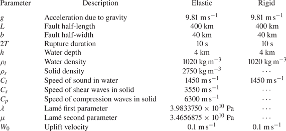
6.2. Surface waves
Consider now the surface waves generated by the single slender fault with parameters as per table 2. The equations generating the surface waves are (3.93) for the elastic case and (3.23) of Williams et al. (Reference Williams, Kadri and Abdolali2021) for the rigid case. At a depth of  $h=4000$ m there is little difference between elastic and rigid cases (figure 17a), but at a depth of $h=1000$ m differences are more apparent (figure 17b). In deeper water the surface wave is almost unaffected by the elasticity of the seabed (Eyov Reference Eyov2013). This surface wave is the main tsunami, i.e. mode 01.
Surface elevation comparison (elastic versus rigid). Coordinates are  $x=1000$ km, $y=0$ km. Coordinate origin at fault centroid. Depths (a) $h=4000$ m and (b) $h=1000$ m.

When the seabed is elastic the possibility of a second surface wave arises. This wave does not exist for all frequencies and never exists in the rigid case (Eyov Reference Eyov2013). The gradient condition (3.66) has to be satisfied before mode 00 can propagate (see figure 18). The mode 00 surface wave has a phase velocity  $C_{l}$, and a negligible amplitude, of the order of micrometres. A plot of mode 00 under the conditions of table 2 can be found in figure 19. In the plot there are four distinct peaks numbered 1 to 4. These peaks in the mode 00 surface wave correspond to the peaks numbered 1, 2, 3 and 4 found in the acoustic signal. The assumption of a rectangular fault moving at a uniform speed results in symmetric peaks, whereas in reality the motion is much more complicated thus upsetting the symmetry of the peaks seen in figure 19.
Left-hand side (LHS) of dispersion relation (3.44) (dashed trace) and right-hand side (RHS) of dispersion relation (solid trace) when  $r\in \mathbb {R}$. The frequency is at the point where mode 00 becomes active, $\omega \simeq 6.95\ \textrm {rad s}^{-1}$, $h=4000$ m (see table 1). The top logarithmic plot indicates overall behaviour. The middle and bottom plots provide expanded views. The mode 00 solution in the middle plot is where the solid curve touches the dashed curve $0\leq r\leq 0.1$, and the mode 01 solution (the usual tsunami) in the bottom plot is where the solid curve again makes contact with the dashed curve in the descending phase $2.5 \leq r \leq 3$.

Mode 00 surface–gravity wave with envelope.

6.3. Hydrophone recordings
The theory developed in this paper leading to the equations for pressure (3.92) and surface elevation (3.93) is linear. Therefore, as in Williams et al. (Reference Williams, Kadri and Abdolali2021), more complicated multi-fault scenarios can be constructed from single slender fault solutions by linear superposition, given that the parameters for each individual fault are known. To contrast the case of an elastic seabed with that of a rigid seabed we revisit the Sumatra 2004 earthquake discussed in § 5.1.2 of Williams et al. (Reference Williams, Kadri and Abdolali2021). The geographical area considered here ranges over [ $70^{\circ }$ to $100^{\circ }$] E longitude and [ $-15^{\circ }$ to $20^{\circ }$] N latitude. This curved patch on the (idealised) spherical Earth is mapped to flat $x, y$ coordinates. The conversion factor of metres per degree is fixed for the latitude ( $y$) direction, but the metres per degree in the longitudinal ( $x$) direction varies with latitude, being maximum at the equator and decreasing as the poles are approached. To simplify the calculations an average value for metres per degree longitude was used and the area considered was kept reasonably small.
The fault centroids are marked by black stars in figures 20(a) and 20(b) and all faults are contained within the masked off ‘earthquake zone’. The purpose of the earthquake zone was to avoid pressure calculations too close to the faults. The location of hydrophone H08N is marked with a red star. Figure 20 indicates the time evolution of the bottom pressure signal for both rigid and elastic seabeds. The elastic seabed has pressure signals already close to the hydrophone at  $t=1000$ s, whereas the rigid seabed only has pressure signals local to the earthquake zone at this time. This is due to the twin effects of a boost in phase velocity for frequencies close to critical in the elastic case and the absence of signal ahead of the main pulse in the rigid stationary phase model. As time proceeds the pressure signals for the elastic case can be seen to traverse the area considered, so that by $t=3625$ s the area is largely clear of pressure oscillations. In contrast, the rigid stationary phase model shows persistent and ever-increasing pressure oscillations around the earthquake zone. The elastic seabed could therefore be considered more physically realistic.
Bottom pressure comparison between rigid and elastic seabed. The location of H08N hydrophone is indicated by a red star at bottom left of each panel. By 3625 s, the elastic model has largely cleared of acoustic–gravity waves whereas the rigid model still has strong oscillations around the earthquake zone. (a) Rigid seabed, bottom pressure map calculated at nine time intervals after first fault movement. (b) Elastic seabed, bottom pressure map calculated at the same time intervals.

Figure 21 compares the predictions made by the elastic seabed model against recorded data for the Sumatra event derived from the southern (H08S1) hydrophone and the seismograph at nearby Diego Garcia (DGAR). The signals recorded by the three hydrophones at station H08S were very similar to each other, and so only that of H08S1 is displayed in the plots (similarly for station H08N). The amplitude of the main acoustic–gravity wave signal for the northern triad is much smaller than that of the southern triad – possibly due to the shielding effect of the Chagos Archipelago (see figures 22a and 23). However, the leading pulses ( $P$-waves) are of similar amplitude. This suggests that the detection of the $P$-waves by the hydrophones is largely unaffected by the presence of the island – unlike signals that travel only through the water. The hydrophone data were obtained from the Comprehensive Nuclear Test Ban Treaty Organisation (CTBTO) and the seismic data from the Incorporated Research Institutions for Seismology (IRIS). The fault configuration is that of table 3/figure 6(a) (Williams et al. Reference Williams, Kadri and Abdolali2021) and the start time given by the United States Geological Survey (USGS) website is UTC 2004-12-26 00:58:53, which corresponds to $t=0$. In the plots the blue vertical lines correspond to the expected arrival time of acoustic–gravity waves travelling at a phase speed of $1450\ \textrm {m s}^{-1}$. The green vertical lines correspond to acoustic–gravity waves travelling at a phase speed of $C_{s}=3550\ \textrm {m s}^{-1}$ and the red vertical lines correspond to a phase speed of $\simeq 8000\ \textrm {m s}^{-1}$. The DGAR seismometer records small-amplitude $P$-waves arriving at the red vertical line, which then transition to larger-amplitude $S$-waves at the green line. The hydrophone H08S weakly detects the $P$-wave activity. The seismic $S$-waves do not exist in the liquid (no shear). The main acoustic–gravity wave signal then arrives and is detected by the hydrophone at the blue line. The re-scaled plot of the hydrophone signal shows this behaviour more clearly. Since $C_{s}$ is the speed limit for the acoustic–gravity waves in the elastic model, the model is unable to predict the $P$-wave portion of the hydrophone signal. Modifications to the existing model or maybe a new model would be needed to capture this behaviour. Between the green and blue lines the elastic model predicts acoustic–gravity waves that can travel at phase speeds close to $C_{s}$ for some frequencies. The hydrophones show weak signal in this region, possibly due to the filtering effect of the hydrophone's response. After the blue line the elastic model predicts a signal that is close in amplitude to that of the hydrophone recordings, but decays more slowly – possibly due to a lack of dissipation included in the model. However, the signal duration is at least finite in the elastic case. There are processes missing from the elastic model (varying bathymetry, reflection, refraction, dissipation etc.) so an exact match is not expected. Examination of figure 21 shows the arrival times for $P$-waves, $S$-waves and the main acoustic–gravity wave pulse (travelling at a phase speed of $C_{l}$) are consistent with our assumptions of constant water density, constant speed of sound in liquid and constant speed of propagation in solid. The leading pulse seen in the hydrophone recordings is primarily made up of lower-frequency components. To show this, a band-pass filter was applied to the hydrophone recording at H08S. The filter eliminates most of the frequency components below 3 Hz and has largely flattened the leading pulse of the H08S signal (figure 24). In order to enhance the detection of acoustic signal between the red and blue lines, ultralow-frequency hydrophones should be used.
Comparison of the current elastic model with both hydrophone and seismic data for the Sumatra 2004 event. The time axis begins at UTC 2004-12-26 00:58:53 ( $t=0$). The vertical red line represents the arrival time for a propagation speed of $8000\ \textrm {m s}^{-1}$, the vertical green line represents the arrival time for a propagation speed of $C_{s} = 3550\ \textrm {m s}^{-1}$ and the vertical blue line represents the arrival time for a propagation speed of $C_{l}=1450 \ \textrm {m s}^{-1}$.

(a) Locations for the H08N and H08S hydrophone triads, along with the DGAR seismograph (yellow markers). The northern triad is shielded by the Chagos Archipelago. (b) Expanded view of island and west coast of Sumatra. Images from Google Earth.

(a,b) Overlay of elastic model prediction onto hydrophone data of north and south locations. (c,d) North and south hydrophone data with re-scaled vertical axis. Red vertical line, arrival time for phase speed  $8000\ \textrm {m s}^{-1}$; green vertical line, arrival time for phase speed $C_{s} = 3550\ \textrm {m s}^{-1}$; blue vertical line, arrival time for phase speed $C_{l} = 1450\ \textrm {m s}^{-1}$.

Leading pulse of hydrophone signal is largely made up of low-frequency components which filtering is able to suppress.

Comparison of two key fault parameters (rupture duration and width) obtained by different methods. The second column ( $\Delta t_{1,2,3,4}$) reports data obtained by filtering the H11 hydrophone signal and measuring timings between peaks. The third column reports data obtained by the methods described within Gomez (Reference Gomez2022). The data in the fourth column are estimates derived from the USGS website.

To demonstrate the extraction of fault timing and geometry from acoustic–gravity wave signals a band-pass filter was applied to the data obtained from hydrophone H11 located at Wake Island during the Samoa 2009 event (data supplied by CTBTO). The timings for the peaks are  $\Delta t_{12}=15.46$, $\Delta t_{34}=27.75$, $\Delta t_{13}=29.89$ and $\Delta t_{24}=42.18\,\textrm {s}$ (figure 25). Note that the time axis in figure 25 does not begin from the start of the rupture. The time axis in this case represents an 1800 s window around the main hydrophone signal. This is not a concern here since only time differences ( $\Delta t$ values) are required. Unlike in the synthetic case this event is asymmetric in the sense that the timings suggest either a trapezoidal rupture geometry or non-uniform uplift velocity (or both). The time $\Delta t_{12}=15.46$ s represents the uplift time for the leading edge of the fault. Assuming that the front and back edges of the fault begin moving together, then $\Delta t_{13}=29.89$ s represents the time for the acoustic signal to travel from the back of the fault, across the fault width, to the front and thus indicates a fault width of $2b=C_{l}\Delta t_{13}\equiv 43.3$ km. The time $\Delta t_{34}=27.75$ s represents the total time for the fault movement (the back end continues moving after the front has stopped). These data compare quite well with those retrieved via inverse modelling in Gomez (Reference Gomez2022). Also, the fault width and timing are approximately those found in the USGS finite fault model (see figure 26) at https://earthquake.usgs.gov/earthquakes/eventpage/usp000h1ys/executive.
(a) Recorded hydrophone data from H11 at Wake Island for Samoa 2009 event. Note that  $t=0$ does not correspond to the rupture start time. (b) Signal after application of band-pass filtering, focusing on the time interval containing the initiation of the main pulse. Data sampling occurs at 250 Hz (one sample every 4 ms).

The USGS finite fault model dimensions and timings. (a) The USGS finite fault model for Samoa 2009 event with scale at bottom left corner. Rectangular region shown is approximately  $30\ \textrm {km} \times 180\ \textrm {km}$. (b) The USGS moment rate function for Samoa 2009 event. The main peak ends between 25 and 35 s.

6.4. The DART buoy data
For the validation of the surface wave calculations against real data we consider the Tohoku event of March 2011 as covered in Williams et al. (Reference Williams, Kadri and Abdolali2021). The parameters used in the elastic model of this paper were changed slightly from those found in Williams et al. (Reference Williams, Kadri and Abdolali2021) and are listed in table 4. In Williams et al. (Reference Williams, Kadri and Abdolali2021) the event was treated as a multi-fault event, so as to capture the main tsunami. However, this paper uses the elastic model and the middle term of (3.93), integrated directly to describe the tsunami (mode 01). It was not necessary to split the fault into a number of faults. By integrating directly the tsunami could be modelled by a single fault. The main peak of the tsunami is described quite well by the elastic model, in terms of both timing and amplitude (see figure 27).
Constants and parameters used in the calculation of surface elevation at DART buoy 21418 for Tohoku 2011 event – elastic model. Also refer to Williams et al. (Reference Williams, Kadri and Abdolali2021).

Surface elevations compared for Tohoku 2011 event at DART buoy 21418.

7. Discussion/summary
We have developed a new mathematical model which combines ground movement of a rectangular slender fault with the properties of an elastic seabed. The model derives expressions for the velocity potential in the liquid, along with dilation potential and rotation potential for the solid. From the liquid velocity potential, we derived expressions for the dynamic pressure (acoustic–gravity waves) and the surface elevation. Far-field behaviour is described by envelope functions containing Fresnel integrals. Elasticity has been shown to be an important consideration when calculating tsunami and acoustic–gravity wave arrival times (Abdolali et al. Reference Abdolali, Kirby and Bellotti2015, Reference Abdolali, Kadri and Kirby2019; Kadri Reference Kadri2019). The model developed in this paper demonstrates the capacity for the acoustic–gravity waves to travel at speeds near the shear wave velocity for frequencies close to critical. Examination of hydrophone data for the Sumatra 2004 event at H08N and H08S locations revealed a leading acoustic signal travelling ahead of the main acoustic–gravity waves at phase speeds in excess of the shear wave velocity  $C_{s}$. The elastic model developed in Eyov et al. (Reference Eyov, Klar, Kadri and Stiassnie2013) and applied in this paper has $C_{s}$ as the speed limit for acoustic–gravity waves, and so does not describe the leading signal in its entirety. Future work could involve modification to the present model, or development of a new elastic model to remedy this.
The tsunami profile is affected by seabed elasticity in shallower water. The inclusion of elasticity induces a decay into the acoustic–gravity wave signals so that the signals terminate after some finite time, unlike the rigid, stationary phase model. From the parameters studied, we find that the signal duration is most affected by the seabed rigidity, with duration increasing alongside rigidity until the totally rigid condition is achieved, at which point the signals persist indefinitely. Thus the inclusion of elasticity helps facilitate a more realistic representation of the pressure field. When the seabed is elastic there exists the possibility of two surface waves. The first (mode 01) is the usual tsunami, but the second (mode 00) is an interesting mode which does not propagate for all frequencies in the elastic case, and never exists in the rigid case. Linear relationships between mode 00 timing of signal peaks and the fault parameters  $b$ (half-width) and $\tau$ (rupture duration) are found and explained. There is also a linear relationship between uplift velocity and mode 00 amplitude. Information on the fault geometry and timing is encoded into the mode 00 surface wave, and is also found to be imprinted into the acoustic–gravity wave signals as well. With appropriate filtering it is possible to extract this information from the acoustic–gravity wave signal (at least in some instances), which would be helpful in solving the inverse problem of deriving fault properties from acoustic/seismic information. Additionally, an improved estimate of the critical cut-off frequency for acoustic modes $n\ge 2$ is presented, which is then used in a new method for calculating approximate phase velocity curves which does not rely on solving the dispersion relation (3.44) at each point. The facility to quickly produce approximate phase velocity curves may help in reducing the computational burden in real-time analysis. In a side-by-side comparison of the shearing method against the dispersion solving method, the shearing method was found to be approximately twice as fast. The comparison was run on the same computer (Intel(R) i9 CPU, 3.60 GHz, 128 GB RAM) and used the same software (Maple) to produce phase velocity curves for 16 modes with $\omega =20\ \textrm {m s}^{-1}$ and depth $h=4000$ m. An approximation for the mode 00 surface wave cut-off frequency is also derived. As in many previous studies, the model developed here has a constant water depth assumption, so while the model can determine the tsunami properties for deep water, it may fail for varying bathymetry. It remains to develop techniques that can account for changes in bathymetry without computation of the entire three-dimensional domain. For slowly varying bathymetry (i.e. mild slopes where $\nabla h(x,y,t)\ll kh$) there already exist techniques in the form of the depth-integrated equations (Sammarco et al. Reference Sammarco, Cecioni, Bellotti and Abdolali2013; Abdolali et al. Reference Abdolali, Kirby and Bellotti2015; Renzi Reference Renzi2017). In the conclusion to Renzi (Reference Renzi2017) the authors remark that models of tsunamigenic events over an elastic seabed do not appear in the literature to date. This topic is addressed and solved (at least for constant depth) in § 3 of this paper.
In the study of the bottom pressure field for the Sumatra 2004 event covered in § 6, a curved patch of the Earth's surface was mapped to a flat  $x,y$ plane. An interesting extension to this work could be to move the perspective of the study into a more global viewpoint by use of spherical coordinates. In that way far-field predictions may become more accurate.
Acknowledgements
All seismic data were downloaded through the IRIS Wilber 3 system (https://ds.iris.edu/wilber3/) or IRIS Web Services (https://service.iris.edu/), including the following seismic networks: (1) the AZ (ANZA; UC San Diego, 1982); (2) the TA (Transportable Array; IRIS, 2003); (3) the US (USNSN, Albuquerque, 1990); (4) the IU (GSN; Albuquerque, 1988).
Declaration of interests
The authors report no conflict of interest.
Disclaimer
The Provisional Technical Secretariat (PTS) of the Commission for the Comprehensive Nuclear Test Ban Treaty Organisation (CTBTO) is not responsible for the views of the authors.
Appendix A. Derivative terms from § 3.4
 \begin{align} & \left.\frac{\partial
H_{2}}{\partial k}\right|_{k=k_{n}}=
\left[\left[-\frac{2\textrm{i}
k_{n}^3\omega^2r_{n}}{q_{n}}\left(\mu
s_{n}+\frac{\rho_{l}g}{2} \right)-4\textrm{i}
q_{n}k_{n}\omega^2r_{n}\left(\mu s_{n}
+\frac{\rho_{l}g}{2}\right) +\frac{2\textrm{i}
q_{n}k_{n}^3\omega^2}{r_{n}}\left(\mu s_{n}
+\frac{\rho_{l}g}{2}\right)\right.\right.\nonumber\\ &\quad
-\frac{2\textrm{i}
q_{n}k_{n}^3\omega^2r_{n}\mu}{s_{n}}+4\textrm{i}
k_{n}\omega^2r_{n}\left(\left(\mu
+\frac{\lambda}{2}\right)q_{n}^2+\frac{\rho_{l}g
q_{n}}{2}-\frac{\lambda k_{n}^2}{2} \right)-\textrm{i}
k_{n} \left(k_{n}^2+s_{n}^2
\right)\frac{\omega^2}{r_{n}}\left(\left(\mu
+\frac{\lambda}{2}\right)q_{n}^2+\frac{\rho_{l}g
q_{n}}{2}-\frac{\lambda k_{n}^2}{2} \right)\nonumber\\ &\quad \left. +\textrm{i} (k_{n}^2+s_{n}^2
)\omega^2r_{n}\left(2k_{n}\left(\mu
+\frac{\lambda}{2}\right)+\frac{\rho_{l}g
k_{n}}{2q_{n}}-\lambda k_{n}
\right)\right]\textrm{e}^{{-}q_{n}}\nonumber\\ &\quad
-\left({-}2\textrm{i} q_{n}k_{n}^2\omega^2r_{n}\left(\mu
s_{n}+\frac{\rho_{l}g}{2} \right) +\textrm{i}
\left(k_{n}^2+s_{n}^2 \right)\omega^2r_{n}\left(\left(\mu
+\frac{\lambda}{2}\right)q_{n}^2+\frac{\rho_{l}g
q_{n}}{2}-\frac{\lambda k_{n}^2}{2} \right)\right)\frac{h
k_{n}\,\textrm{e}^{{-}q_{n}h}}{q_{n}}\nonumber\\ &\quad
\left. -\textrm{i}\left(2q_{n}k_{n}^2\left(-\mu gr_{n}^2
s_{n}+\frac{\rho_{l}\omega^4}{2}\right)
-\left(k_{n}^2+s_{n}^2 \right)\left({-}g
r_{n}^2\left(\mu+\frac{\lambda}{2}\right)q_{n}^2 +
\frac{\rho_{l}\omega^4q_{n}}{2}+\frac{g r_{n}^2\lambda
k_{n}^2}{2} \right)\right)\frac{\textrm{e}^{{-}q_{n}h}h
k_{n}}{r_{n}}\right]\cos\left(r_{n}h \right)\nonumber\\ &\quad
+\left[\textrm{i}\left[\frac{2k_{n}^3}{q_{n}}\left(-\mu g
r_{n}^2s_{n}+\frac{\rho_{l}\omega^4}{2}\right)+4q_{n}k_{n}\left(-\mu
g r_{n}^2s_{n}+\frac{\rho_{l}\omega^4}{2}
\right)+2q_{n}k_{n}^2\left(2\mu g k_{n}s_{n}-\frac{\mu g
r_{n}^2k_{n}}{s_{n}} \right) \right.\right.\nonumber\\ &\quad -4k_{n}\left({-}g
r_{n}^2\left(\mu+\frac{\lambda}{2}\right)q_{n}^2+\frac{\rho_{l}\omega^4q_{n}}{2}+\frac{g
r_{n}^2\lambda k_{n}^2}{2}\right)\nonumber\\ &\quad
\left.-(k_{n}^2+s_{n}^2)\left(2g
k_{n}\left(\mu+\frac{\lambda}{2}\right)q_{n}^2-2g
r_{n}^2\left(\mu+\frac{\lambda}{2}\right)k_{n}+\frac{\rho_{l}\omega^4k_{n}}{2q_{n}}-g
k_{n}^3\lambda+g r_{n}^2\lambda
k_{n}\right)\right]\textrm{e}^{{-}q_{n}}\nonumber\\ &\quad
+\left({-}2\textrm{i} q_{n}k_{n}^2\omega^2r_{n}\left(\mu
s_{n}+\frac{\rho_{l}g}{2}\right)+\textrm{i}(k_{n}^2+s_{n}^2)\omega^2r_{n}\left(\left(\mu+\frac{\lambda}{2}\right)q_{n}^2+\frac{\rho_{l}g
q_{n}}{2}-\frac{\lambda k_{n}^2}{2} \right)
\right)\frac{\textrm{e}^{{-}q_{n}h}h
k_{n}}{r_{n}}\nonumber\\ &\quad
\left.-\textrm{i}\left(2q_{n}k_{n}^2\left(-\mu g
r_{n}^2s_{n}+\frac{\rho_{l}\omega^4}{2}\right)-(k_{n}^2+s_{n}^2)\left({-}g
r_{n}^2\left(\mu+\frac{\lambda}{2}\right)q_{n}^2+\frac{\rho_{l}\omega^4q_{n}}{2}+\frac{g
r_{n}^2\lambda k_{n}^2}{2}\right)\right)\frac{h
k_{n}\,\textrm{e}^{{-}q_{n}h}}{q_{n}}\right]\sin(r_{n}h),
\end{align}
\begin{align} & \left.\frac{\partial
H_{2}}{\partial k}\right|_{k=k_{n}}=
\left[\left[-\frac{2\textrm{i}
k_{n}^3\omega^2r_{n}}{q_{n}}\left(\mu
s_{n}+\frac{\rho_{l}g}{2} \right)-4\textrm{i}
q_{n}k_{n}\omega^2r_{n}\left(\mu s_{n}
+\frac{\rho_{l}g}{2}\right) +\frac{2\textrm{i}
q_{n}k_{n}^3\omega^2}{r_{n}}\left(\mu s_{n}
+\frac{\rho_{l}g}{2}\right)\right.\right.\nonumber\\ &\quad
-\frac{2\textrm{i}
q_{n}k_{n}^3\omega^2r_{n}\mu}{s_{n}}+4\textrm{i}
k_{n}\omega^2r_{n}\left(\left(\mu
+\frac{\lambda}{2}\right)q_{n}^2+\frac{\rho_{l}g
q_{n}}{2}-\frac{\lambda k_{n}^2}{2} \right)-\textrm{i}
k_{n} \left(k_{n}^2+s_{n}^2
\right)\frac{\omega^2}{r_{n}}\left(\left(\mu
+\frac{\lambda}{2}\right)q_{n}^2+\frac{\rho_{l}g
q_{n}}{2}-\frac{\lambda k_{n}^2}{2} \right)\nonumber\\ &\quad \left. +\textrm{i} (k_{n}^2+s_{n}^2
)\omega^2r_{n}\left(2k_{n}\left(\mu
+\frac{\lambda}{2}\right)+\frac{\rho_{l}g
k_{n}}{2q_{n}}-\lambda k_{n}
\right)\right]\textrm{e}^{{-}q_{n}}\nonumber\\ &\quad
-\left({-}2\textrm{i} q_{n}k_{n}^2\omega^2r_{n}\left(\mu
s_{n}+\frac{\rho_{l}g}{2} \right) +\textrm{i}
\left(k_{n}^2+s_{n}^2 \right)\omega^2r_{n}\left(\left(\mu
+\frac{\lambda}{2}\right)q_{n}^2+\frac{\rho_{l}g
q_{n}}{2}-\frac{\lambda k_{n}^2}{2} \right)\right)\frac{h
k_{n}\,\textrm{e}^{{-}q_{n}h}}{q_{n}}\nonumber\\ &\quad
\left. -\textrm{i}\left(2q_{n}k_{n}^2\left(-\mu gr_{n}^2
s_{n}+\frac{\rho_{l}\omega^4}{2}\right)
-\left(k_{n}^2+s_{n}^2 \right)\left({-}g
r_{n}^2\left(\mu+\frac{\lambda}{2}\right)q_{n}^2 +
\frac{\rho_{l}\omega^4q_{n}}{2}+\frac{g r_{n}^2\lambda
k_{n}^2}{2} \right)\right)\frac{\textrm{e}^{{-}q_{n}h}h
k_{n}}{r_{n}}\right]\cos\left(r_{n}h \right)\nonumber\\ &\quad
+\left[\textrm{i}\left[\frac{2k_{n}^3}{q_{n}}\left(-\mu g
r_{n}^2s_{n}+\frac{\rho_{l}\omega^4}{2}\right)+4q_{n}k_{n}\left(-\mu
g r_{n}^2s_{n}+\frac{\rho_{l}\omega^4}{2}
\right)+2q_{n}k_{n}^2\left(2\mu g k_{n}s_{n}-\frac{\mu g
r_{n}^2k_{n}}{s_{n}} \right) \right.\right.\nonumber\\ &\quad -4k_{n}\left({-}g
r_{n}^2\left(\mu+\frac{\lambda}{2}\right)q_{n}^2+\frac{\rho_{l}\omega^4q_{n}}{2}+\frac{g
r_{n}^2\lambda k_{n}^2}{2}\right)\nonumber\\ &\quad
\left.-(k_{n}^2+s_{n}^2)\left(2g
k_{n}\left(\mu+\frac{\lambda}{2}\right)q_{n}^2-2g
r_{n}^2\left(\mu+\frac{\lambda}{2}\right)k_{n}+\frac{\rho_{l}\omega^4k_{n}}{2q_{n}}-g
k_{n}^3\lambda+g r_{n}^2\lambda
k_{n}\right)\right]\textrm{e}^{{-}q_{n}}\nonumber\\ &\quad
+\left({-}2\textrm{i} q_{n}k_{n}^2\omega^2r_{n}\left(\mu
s_{n}+\frac{\rho_{l}g}{2}\right)+\textrm{i}(k_{n}^2+s_{n}^2)\omega^2r_{n}\left(\left(\mu+\frac{\lambda}{2}\right)q_{n}^2+\frac{\rho_{l}g
q_{n}}{2}-\frac{\lambda k_{n}^2}{2} \right)
\right)\frac{\textrm{e}^{{-}q_{n}h}h
k_{n}}{r_{n}}\nonumber\\ &\quad
\left.-\textrm{i}\left(2q_{n}k_{n}^2\left(-\mu g
r_{n}^2s_{n}+\frac{\rho_{l}\omega^4}{2}\right)-(k_{n}^2+s_{n}^2)\left({-}g
r_{n}^2\left(\mu+\frac{\lambda}{2}\right)q_{n}^2+\frac{\rho_{l}\omega^4q_{n}}{2}+\frac{g
r_{n}^2\lambda k_{n}^2}{2}\right)\right)\frac{h
k_{n}\,\textrm{e}^{{-}q_{n}h}}{q_{n}}\right]\sin(r_{n}h),
\end{align}
 \begin{equation} \left.\frac{\partial H_{2}}{\partial k}\right|_{k={-}k_{n}}=\left.\frac{\partial H_{2}}{\partial k}\right|_{k=k_{n}}\!, \end{equation}
 \begin{align} &\left.\frac{\partial H_{2}}{\partial k}\right|_{k=\textrm{i}\varLambda_{n}}=\left[\left[-\frac{2\varLambda_{n}^3\omega^2r_{n}}{q_{n}}\left(\mu s_{n}+\frac{\rho_{l}g}{2}\right)+4q_{n}\varLambda_{n}\omega^2r_{n}\left(\mu s_{n}+\frac{\rho_{l}g}{2}\right)+\frac{2q_{n}\varLambda_{n}^3\omega^2}{r_{n}}\left(\mu s_{n}+\frac{\rho_{l}g}{2}\right)\right.\right.\nonumber\\ &\quad -\frac{2q_{n}\varLambda_{n}^3\omega^2r_{n}\mu}{s_{n}}-4\varLambda_{n}\omega^2r_{n}\left(\left(\mu+\frac{\lambda}{2}\right)q_{n}^2+\frac{\rho_{l}g q_{n}}{2}+\frac{\lambda\varLambda_{n}^2}{2}\right)+\left(-\varLambda_{n}^2+s_{n}^2 \right)\frac{\omega^2}{r_{n}}\left(\left(\mu+\frac{\lambda}{2}\right)q_{n}^2+\frac{\rho_{l}g q_{n}}{2}+\frac{\lambda\varLambda_{n}^2}{2}\right)\varLambda_{n}\nonumber\\ &\quad \left.+\textrm{i}\left(-\varLambda_{n}^2+s_{n}^2\right)\omega^2r_{n}\left(2\textrm{i} \varLambda_{n}\left(\mu+\frac{\lambda}{2}\right)+\frac{\textrm{i}\rho_{l}g\varLambda_{n}}{2q_{n}}-\textrm{i}\lambda\varLambda_{n} \right)\right]\textrm{e}^{{-}q_{n}h}\nonumber\\ &\quad -\textrm{i}\left(2\textrm{i} q_{n}\varLambda_{n}^2\omega^2r_{n}\left(\mu s_{n}+\frac{\rho_{l}g}{2}\right)+\textrm{i}\left(-\varLambda_{n}^2+s_{n}^2 \right)\omega^2r_{n}\left(\left(\mu+\frac{\lambda}{2}\right)q_{n}^2+\frac{\rho_{l}g q_{n}}{2}+\frac{\lambda\varLambda_{n}^2}{2}\right) \right)\frac{h\varLambda_{n}\,\textrm{e}^{{-}q_{n}h}}{q_{n}}\nonumber\\ &\quad \left. +\left({-}2q_{n}\varLambda_{n}^2\left(-\mu g r_{n}^2s_{n}+\frac{\rho_{l}\omega^4}{2} \right)-\left(-\varLambda_{n}^2+s_{n}^2\right)\left({-}g r_{n}^2\left(\mu+\frac{\lambda}{2} \right)q_{n}^2+\frac{\rho_{l}\omega^4q_{n}}{2}-\frac{g r_{n}^2\lambda\varLambda_{n}^2}{2} \right) \right)\frac{h\varLambda_{n}\,\textrm{e}^{{-}q_{n}h}}{r_{n}} \right]\cos\left(r_{n}h\right)\nonumber\\ &\quad +\left[\textrm{i}\left[-\frac{2\textrm{i}\varLambda_{n}^3}{q_{n}}\left(-\mu g r_{n}^2s_{n}+\frac{\rho_{l}\omega^4}{2}\right)+4\textrm{i} q_{n}\varLambda_{n}\left(-\mu g r_{n}^2s_{n}+\frac{\rho_{l}\omega^4}{2}\right)-2q_{n}\varLambda_{n}^2\left(2\textrm{i} \mu g\varLambda_{n}s_{n}-\frac{\textrm{i}\mu g r_{n}^2\varLambda_{n}}{s_{n}}\right)\right.\right.\nonumber\\ &\quad -4\textrm{i}\varLambda_{n}\left({-}g r_{n}^2\left(\mu+\frac{\lambda}{2}\right)q_{n}^2+\frac{\rho_{l}\omega^4q_{n}}{2}-\frac{g r_{n}^2\lambda\varLambda_{n}^2}{2}\right)\nonumber\\ &\quad \left.-\left(-\varLambda_{n}^2+s_{n}^2\right)\left(2\textrm{i} g\varLambda_{n}\left(\mu+\frac{\lambda}{2}\right)q_{n}^2-2\textrm{i} g r_{n}^2\left(\mu+\frac{\lambda}{2}\right)\varLambda_{n}+\frac{\textrm{i}\rho_{l}\omega^4\varLambda_{n}}{2q_{n}}+g\varLambda_{n}^3\lambda\textrm{i}+g r_{n}^2\lambda\varLambda_{n}\textrm{i}\right) \right]\textrm{e}^{{-}q_{n}h}\nonumber\\ &\quad +\textrm{i}\left(2\textrm{i} q_{n}\varLambda_{n}^2\omega^2r_{n}\left(\mu s_{n}+\frac{\rho_{l}g}{2} \right)+\textrm{i}\left(-\varLambda_{n}^2+s_{n}^2\right)\omega^2r_{n}\left(\left(\mu+\frac{\lambda}{2}\right)q_{n}^2+\frac{\rho_{l}g q_{n}}{2}+\frac{\lambda\varLambda_{n}^2}{2}\right) \right)\frac{h\varLambda_{n}\,\textrm{e}^{{-}q_{n}h}}{r_{n}}\nonumber\\ &\quad \left.+\left({-}2q_{n}\varLambda_{n}^2\left(-\mu g r_{n}^2s_{n}+\frac{\rho_{l}\omega^4}{2} \right)-\left(-\varLambda_{n}^2+s_{n}^2\right)\left({-}g r_{n}^2\left(\mu+\frac{\lambda}{2} \right)q_{n}^2+\frac{\rho_{l}\omega^4q_{n}}{2}-\frac{g r_{n}^2\lambda\varLambda_{n}^2}{2} \right) \right)\frac{h\varLambda_{n}\,\textrm{e}^{{-}q_{n}h}}{q_{n}}\right]\sin\left(r_{n}h\right), \end{align}
 \begin{align} & \left.\frac{\partial H_{2}}{\partial k}\right|_{k=k_{0m}}=\left[\left[-\frac{2k_{0m}^3\omega^2r_{0m}}{q_{0m}}\left(\mu s_{0m}+\frac{\rho_{l}g}{2}\right)-4q_{0m}k_{0m}\omega^2r_{0m}\left(\mu s_{0m}+\frac{\rho_{l}g}{2}\right)-\frac{2q_{0m}k_{0m}^3\omega^2}{r_{0m}}\left(\mu s_{0m}+\frac{\rho_{l}g}{2}\right)\right.\right.\nonumber\\ &\quad -\frac{2q_{0m}k_{0m}^3\omega^2r_{0m}\mu}{s_{0m}}+4k_{0m}\omega^2r_{0m}\left(\left(\mu+\frac{\lambda}{2}\right)q_{0m}^2+\frac{\rho_{l}g q_{0m}}{2}-\frac{\lambda k_{0m}^2}{2}\right)\nonumber\\ &\quad+\left(k_{0m}^2+s_{0m}^2\right)\frac{\omega^2k_{0m}}{r_{0m}}\left(\left(\mu+\frac{\lambda}{2}\right)q_{0m}^2+\frac{\rho_{l}g q_{0m}}{2}-\frac{\lambda k_{0m}^2}{2}\right)\nonumber\\ &\quad\left.+\left(k_{0m}^2+s_{0m}^2\right)\omega^2r_{0m}\left(2k_{0m}\left(\mu+\frac{\lambda}{2}\right)+\frac{\rho_{l}g k_{0m}}{2q_{0m}}-\lambda k_{0m}\right)\right]\textrm{e}^{{-}q_{0m}h}\nonumber\\ &\quad -\left({-}2q_{0m}k_{0m}^2\omega^2r_{0m}\left(\mu s_{0m}+\frac{\rho_{l}g}{2}\right)+\left(k_{0m}^2+s_{0m}^2\right)\omega^2r_{0m}\left(\left(\mu+\frac{\lambda}{2}\right)q_{0m}^2+\frac{\rho_{l}g q_{0m}}{2}-\frac{\lambda k_{0m}^2}{2}\right) \right)\frac{h k_{0m}\,\textrm{e}^{{-}q_{0m}h}}{q_{0m}}\nonumber\\ &\quad \left.+\left(2q_{0m}k_{0m}^2\left(\mu g r_{0m}^2s_{0m}+\frac{\rho_{l}\omega^4}{2}\right)-\left(k_{0m}^2+s_{0m}^2\right)\left(g r_{0m}^2\left(\mu+\frac{\lambda}{2}\right)q_{0m}^2+\frac{\rho_{l}\omega^4q_{0m}}{2}-\frac{g r_{0m}^2\lambda k_{0m}^2}{2}\right)\right)\frac{h k_{0m}\,\textrm{e}^{{-}q_{0m}h}}{r_{0m}}\right]\cosh\left(r_{0m}h\right)\nonumber\\ &\quad +\left[\left({-}2q_{0m}k_{0m}^2\omega^2r_{0m}\left(\mu s_{0m}+\frac{\rho_{l}g}{2}\right)+\left(k_{0m}^2+s_{0m}^2\right)\omega^2r_{0m}\left(\left(\mu+\frac{\lambda}{2}\right)q_{0m}^2+\frac{\rho_{l}g q_{0m}}{2}-\frac{\lambda k_{0m}^2}{2}\right) \right)\frac{h k_{0m}\,\textrm{e}^{{-}q_{0m}h}}{r_{0m}}\right.\nonumber\\ &\quad -\left(2q_{0m}k_{0m}^2\left(\mu g r_{0m}^2s_{0m}+\frac{\rho_{l}\omega^4}{2}\right)-\left(k_{0m}^2+s_{0m}^2\right)\left(g r_{0m}^2\left(\mu+\frac{\lambda}{2}\right)q_{0m}^2+\frac{\rho_{l}\omega^4q_{0m}}{2}-\frac{g r_{0m}^2\lambda k_{0m}^2}{2}\right)\right)\frac{h k_{0m}\,\textrm{e}^{{-}q_{0m}h}}{q_{0m}} \nonumber\\ &\quad +\left[\frac{2k_{0m}^3}{q_{0m}}\left(\mu g r_{0m}^2s_{0m}+\frac{\rho_{l}\omega^4}{2} \right)+4q_{0m}k_{0m}\left(\mu g r_{0m}^2s_{0m}+\frac{\rho_{l}\omega^4}{2}\right)+2q_{0m}k_{0m}^2\left(2\mu g k_{0m}s_{0m}+\frac{\mu g r_{0m}^2k_{0m}}{s_{0m}}\right) \right.\nonumber\\ &\quad -4k_{0m}\left(g r_{0m}^2\left(\mu+\frac{\lambda}{2}\right)q_{0m}^2+\frac{\rho_{l}\omega^4q_{0m}}{2}-\frac{g r_{0m}^2\lambda k_{0m}^2}{2}\right)\nonumber\\ &\quad \left.\left.-\left(k_{0m}^2+s_{0m}^2\right)\left(2g k_{0m}\left(\mu+\frac{\lambda}{2} \right)q_{0m}^2+2g r_{0m}^2k_{0m}\left(\mu+\frac{\lambda}{2}\right)+\frac{\rho_{l}\omega^4k_{0m}}{2q_{0m}}-g k_{0m}^3\lambda-g r_{0m}^2\lambda k_{0m} \right)\right]\textrm{e}^{{-}q_{0m}h}\right]\sinh\left(r_{0m})\right), \end{align}
 \begin{equation} \left.\frac{\partial H_{2}}{\partial k}\right|_{k={-}k_{0m}}={-}\left.\frac{\partial H_{2}}{\partial k}\right|_{k=k_{0m}}. \end{equation}
Appendix B. Substitutions from § 4.1
 \begin{align} \tan\left[\left(n-\frac{3}{2}\right){\rm \pi}+\delta\right]= \frac{\displaystyle -4\widetilde{C_{s}}^{2}\left\{ \dfrac{1}{4}\widetilde{C_{p}}^{2}(\widetilde{C_{l}}^{2}- \widetilde{C_{s}}^{2})\sqrt{-\dfrac{(2n{\rm \pi}-3{\rm \pi}+2 \delta)^{2}\widetilde{C_{l}}^{2}(\widetilde{C_{p}}^{2}- \widetilde{C_{s}}^{2})}{\widetilde{C_{p}}^{2} (\widetilde{C_{l}}^{2}-\widetilde{C_{s}}^{2})}}+ \widetilde{C_{l}}^{2}\left[\left(n-\frac{3}{2}\right) {\rm \pi}+\delta\right]^{2}\left[\left(-\tilde{\mu}- \frac{\tilde{\lambda}}{2}\right)\widetilde{C_{s}}^{2}+\tilde{\mu} \widetilde{C_{p}}^{2}\right]\right\} }{\displaystyle \left[\left(n-\frac{3}{2}\right){\rm \pi}+\delta\right]\left\{ \widetilde{C_{s}}^{4}\widetilde{C_{l}}^{2} \widetilde{C_{p}}^{2}\sqrt{-\dfrac{(2n{\rm \pi}-3{\rm \pi} +2\delta)^{2}\widetilde{C_{l}}^{2} (\widetilde{C_{p}}^{2}-\widetilde{C_{s}}^{2})}{\widetilde{C_{p}}^{2} (\widetilde{C_{l}}^{2}-\widetilde{C_{s}}^{2})}}-4 (\widetilde{C_{l}}^{2}-\widetilde{C_{s}}^{2}) \left[\left(-\tilde{\mu}-\frac{\tilde{\lambda}}{2}\right) \widetilde{C_{s}}^{2}+\tilde{\mu} \widetilde{C_{p}}^{2}\right]\right\}}. \end{align}
Appendix C. Coefficients from equation (4.5)
 \begin{equation} \left.\begin{array}{c@{}}
\begin{aligned} a_{n} & ={-}2{\rm \pi}
\widetilde{C_{s}}^{2}\widetilde{C_{p}}^{2}
(\widetilde{C_{l}}^{2}-\widetilde{C_{s}}^{2})
\sqrt{\dfrac{(2n-3)^{2}\widetilde{C_{l}}^{2}
(\widetilde{C_{s}}^{2}-\widetilde{C_{p}}^{2})}{\widetilde{C_{p}}^{2}
(\widetilde{C_{l}}^{2}-\widetilde{C_{s}}^{2})}}\\ & \quad
+4{\rm \pi}^{2}\widetilde{C_{s}}^{2}\widetilde{C_{l}}^{2}
\left(n-\dfrac{3}{2}\right)^{2}[(\tilde{\lambda}
+2\tilde{\mu})\widetilde{C_{s}}^{2}-2\tilde{\mu}
\widetilde{C_{p}}^{2}],\end{aligned}\\
\begin{aligned} b_{n} &
={-}2\widetilde{C_{s}}^{2}\widetilde{C_{p}}^{2}
\dfrac{(\widetilde{C_{l}}^{2}-
\widetilde{C_{s}}^{2})}{\left(n-\dfrac{3}{2}\right)}
\sqrt{\dfrac{(2n-3)^{2}\widetilde{C_{l}}^{2}
(\widetilde{C_{s}}^{2}-\widetilde{C_{p}}^{2})}{\widetilde{C_{p}}^{2}
(\widetilde{C_{l}}^{2}-\widetilde{C_{s}}^{2})}}\\ & \quad
+8{\rm \pi} \widetilde{C_{s}}^{2}\widetilde{C_{l}}^{2}
\left(n-\dfrac{3}{2}\right)[(\tilde{\lambda}+
2\tilde{\mu})\widetilde{C_{s}}^{2}-2\tilde{\mu}
\widetilde{C_{p}}^{2}],\end{aligned}\\
\begin{aligned} c_{n} &
=2\left(n-\dfrac{3}{2}\right){\rm \pi}^{2}\widetilde{C_{s}}^{4}
\widetilde{C_{l}}^{2}\widetilde{C_{p}}^{2}\sqrt{\dfrac{(2n-3)^{2}
\widetilde{C_{l}}^{2}(\widetilde{C_{s}}^{2}-
\widetilde{C_{p}}^{2})}{\widetilde{C_{p}}^{2}
(\widetilde{C_{l}}^{2}-\widetilde{C_{s}}^{2})}}\\ & \quad
+4{\rm \pi} \left(n-\dfrac{3}{2}\right)
(\widetilde{C_{l}}^{2}-\widetilde{C_{s}}^{2})
[(\tilde{\lambda}+2\tilde{\mu})\widetilde{C_{s}}^{2}-2\tilde{\mu}
\widetilde{C_{p}}^{2}],\end{aligned}\\
\begin{aligned} d_{n} & =4{\rm \pi}
\widetilde{C_{s}}^{4}\widetilde{C_{l}}^{2}
\widetilde{C_{p}}^{2}\sqrt{\dfrac{(2n-3)^{2}\widetilde{C_{l}}^{2}
(\widetilde{C_{s}}^{2}-\widetilde{C_{p}}^{2})}{\widetilde{C_{p}}^{2}
(\widetilde{C_{l}}^{2}-\widetilde{C_{s}}^{2})}}\\ & \quad
+4 (\widetilde{C_{l}}^{2}-\widetilde{C_{s}}^{2})
[(\tilde{\lambda}+2\tilde{\mu})\widetilde{C_{s}}^{2}-2\tilde{\mu}
\widetilde{C_{p}}^{2}]. \end{aligned}
\end{array}\right\} \end{equation}
\begin{equation} \left.\begin{array}{c@{}}
\begin{aligned} a_{n} & ={-}2{\rm \pi}
\widetilde{C_{s}}^{2}\widetilde{C_{p}}^{2}
(\widetilde{C_{l}}^{2}-\widetilde{C_{s}}^{2})
\sqrt{\dfrac{(2n-3)^{2}\widetilde{C_{l}}^{2}
(\widetilde{C_{s}}^{2}-\widetilde{C_{p}}^{2})}{\widetilde{C_{p}}^{2}
(\widetilde{C_{l}}^{2}-\widetilde{C_{s}}^{2})}}\\ & \quad
+4{\rm \pi}^{2}\widetilde{C_{s}}^{2}\widetilde{C_{l}}^{2}
\left(n-\dfrac{3}{2}\right)^{2}[(\tilde{\lambda}
+2\tilde{\mu})\widetilde{C_{s}}^{2}-2\tilde{\mu}
\widetilde{C_{p}}^{2}],\end{aligned}\\
\begin{aligned} b_{n} &
={-}2\widetilde{C_{s}}^{2}\widetilde{C_{p}}^{2}
\dfrac{(\widetilde{C_{l}}^{2}-
\widetilde{C_{s}}^{2})}{\left(n-\dfrac{3}{2}\right)}
\sqrt{\dfrac{(2n-3)^{2}\widetilde{C_{l}}^{2}
(\widetilde{C_{s}}^{2}-\widetilde{C_{p}}^{2})}{\widetilde{C_{p}}^{2}
(\widetilde{C_{l}}^{2}-\widetilde{C_{s}}^{2})}}\\ & \quad
+8{\rm \pi} \widetilde{C_{s}}^{2}\widetilde{C_{l}}^{2}
\left(n-\dfrac{3}{2}\right)[(\tilde{\lambda}+
2\tilde{\mu})\widetilde{C_{s}}^{2}-2\tilde{\mu}
\widetilde{C_{p}}^{2}],\end{aligned}\\
\begin{aligned} c_{n} &
=2\left(n-\dfrac{3}{2}\right){\rm \pi}^{2}\widetilde{C_{s}}^{4}
\widetilde{C_{l}}^{2}\widetilde{C_{p}}^{2}\sqrt{\dfrac{(2n-3)^{2}
\widetilde{C_{l}}^{2}(\widetilde{C_{s}}^{2}-
\widetilde{C_{p}}^{2})}{\widetilde{C_{p}}^{2}
(\widetilde{C_{l}}^{2}-\widetilde{C_{s}}^{2})}}\\ & \quad
+4{\rm \pi} \left(n-\dfrac{3}{2}\right)
(\widetilde{C_{l}}^{2}-\widetilde{C_{s}}^{2})
[(\tilde{\lambda}+2\tilde{\mu})\widetilde{C_{s}}^{2}-2\tilde{\mu}
\widetilde{C_{p}}^{2}],\end{aligned}\\
\begin{aligned} d_{n} & =4{\rm \pi}
\widetilde{C_{s}}^{4}\widetilde{C_{l}}^{2}
\widetilde{C_{p}}^{2}\sqrt{\dfrac{(2n-3)^{2}\widetilde{C_{l}}^{2}
(\widetilde{C_{s}}^{2}-\widetilde{C_{p}}^{2})}{\widetilde{C_{p}}^{2}
(\widetilde{C_{l}}^{2}-\widetilde{C_{s}}^{2})}}\\ & \quad
+4 (\widetilde{C_{l}}^{2}-\widetilde{C_{s}}^{2})
[(\tilde{\lambda}+2\tilde{\mu})\widetilde{C_{s}}^{2}-2\tilde{\mu}
\widetilde{C_{p}}^{2}]. \end{aligned}
\end{array}\right\} \end{equation}


 Open access

