1. Introduction
The water entry process describes the rapid transition of an object from air through the free surface into water, involving multiple physical phenomena including cross-medium transport, impact, spray formation, cavity dynamics and structural deformation. This constitutes a classical complex multiphase flow and represents a fluid–structure interaction (FSI) problem. Water entry phenomena are prevalent in aerospace and marine engineering applications, such as biomimetic underwater vehicles (Gan et al. Reference Gan, Zhuang, Zhang, Zuo and Xiang2024), lifeboat deployment (Wang et al. Reference Wang, Liu, Lei, Wu, Wang and Deng2024), ship slamming (Han et al. Reference Han, Li, Guo, Sun and Liu2024) and aircraft ditching (Cui et al. Reference Cui, Zhang, Dong, Jin, Zhang and Zhu2024). Unlike idealised free-surface water entry conditions, ocean environments often contain floating structures such as marine debris, floating ice, plastic waste or other floating objects. These floating structures typically possess structural strength and significantly influence the impact dynamics, cavity evolution and water entry trajectory of projectiles. The multiphase flow characteristics under floating structure constraints, multi-body coupling effects and energy transfer mechanisms remain insufficiently understood. Therefore, systematic investigation of the FSI mechanisms during projectile water entry with floating structure interaction holds both fundamental significance and practical value. Such research contributes to improving the deployment of marine detection equipment and enhancing safety assessments of offshore structures in complex sea conditions.
The scientific investigation of water entry phenomena dates back to the late 19th century, when Worthington (Reference Worthington1883, Reference Worthington and Cole1900, Reference Worthington1909) pioneered the systematic experimental observation of fluid dynamics during the water entry of droplets and spherical bodies using high-speed photography. His work provided a comprehensive description of characteristic flow features, including spray, cavity formation and the subsequent jet development following cavity closure. Subsequently, Mallock (Reference Mallock1918) conducted extensive independent experimental studies focusing on the acoustic field generated during water entry, which not only validated Worthington’s earlier findings, but also further discussed the cavity and splash characteristics of the sphere during high speed water entry, and the relationship between the resistance of the sphere and its density.
The growing demands of marine engineering have shifted the research focus from fundamental studies of water entry phenomena in idealised stationary conditions to more practical investigations involving complex marine environments and dynamic response analyses. Traditional approaches typically assume water entry occurs on a calm, homogeneous free surface without external disturbances. These assumptions, while useful for revealing fundamental physical mechanisms, significantly deviate from real marine conditions. In reality, water entry processes are often influenced by various non-ideal factors, including wave disturbances, floating object interference and flow field inhomogeneity, leading to considerably more complex dynamic response mechanisms. Several studies have addressed water entry problems under complex boundary conditions. Huang et al. (Reference Huang, Wang, Li, Zhang, Chen, Zhao, Xu and Chen2024) systematically investigated how wave height and direction affect cavity evolution and hydrodynamic characteristics during water entry. The results demonstrate that increased wave height promotes cavity expansion and enhances peak impact pressure. Fan, Yao & Ma (Reference Fan, Yao and Ma2024) conducted scaled model experiments under various environmental conditions (including normal and reduced pressure) to examine similarity criteria and load prediction. The study discussed the influence of cavitation number and atmospheric density coefficient on multiphase flow, slamming loads and air cushion effects. Zhang et al. (Reference Zhang, Liu, Ren, Li, Zhang and Lu2024) experimentally studied cavity effects on the water entry stability of vehicles. Findings reveal that cavities near the free surface can reconstruct wave patterns, enabling vehicles to enter water at larger angles while improving underwater motion stability. Rabbi, Mortensen & Kiyama (Reference Rabbi, Mortensen and Kiyama2024) examined asymmetric cavity formation between two adjacent impacting spheres, showing that symmetry breaking alters cavity sealing (deep seal) timing and induces oblique Worthington jet formation. Sui, Han & Wang (Reference Sui, Han and Wang2024) investigated non-axisymmetric cavity dynamics during vertical water entry near side walls, analysing wall effects on closure time and position.
However, this kind of research mostly focuses on fluid field characteristics, treating environmental factors merely as boundary conditions while neglecting the interaction between solids and impact responses. In practical marine operations, underwater equipment such as deep-sea probes, buoys and unmanned submersibles needs to traverse ice fields or debris zones during water entry. These conditions inevitably involve direct contact between the equipment and floating structures, leading to strong coupling between solid impacts and subsequent water entry dynamics. Research on such coupled impact–water entry phenomena remains in its nascent stage, primarily due to the highly complex fluid–structure interaction dynamics involved. This process encompasses not only structural damage and failure evolution of floating objects under impact, but also requires considering the disturbance of broken solids to the local flow field structure and the feedback effect of water on the movement behaviour of broken objects. Regarding modelling approaches, the discrete element method (DEM) has gained widespread application in studies of solid material synthesis and impact failure mechanisms due to its exceptional capability in simulating interparticle contact, fragmentation and reconstruction behaviours. Yang, Xu & Yuan (Reference Yang, Xu and Yuan2025) investigated failure evolution at metal–glass interfaces using DEM, deriving quantitative expressions for strain-rate dependent fracture strain and crack width in metal impactors. Luo, Wu & Wang (Reference Luo, Wu and Wang2025) employed a bonded DEM approach to study critical nanosphere behaviours during thermoforming processes, including bond formation dynamics, plastic deformation and fracture mechanics, revealing how interfacial bonding parameters influence macroscopic mechanical properties. Zuo, Feng & Liu (Reference Zuo, Feng and Liu2025) used DEM to examine aggregate fragmentation under impact, quantifying fracture performance through impact force, fragment size and penetration depth. Bai, Zhou & Mang (Reference Bai, Zhou and Mang2025) developed a DEM-based framework accounting for variations in bonding strength and porosity due to clay loss in filled media. Kushimoto & Kano (Reference Kushimoto and Kano2025) implemented a cross-bonded DEM to analyse particle deformation and failure, where bond units (comprising spring-damper systems) fracture when exceeding critical elongation thresholds. These DEM capabilities demonstrate their suitability for effectively modelling and tracking both floating marine structures and their impact-induced fragmentation processes.
During the impact water entry process, the interaction between fragments and surrounding fluid significantly influences both flow field evolution and hydrodynamic characteristics, while the fluid flow conversely alters the settling trajectories and kinematic states of the fragments. The coupled CFD–DEM approach enables high-precision simulation of fluid–discrete particle interactions and has high applicability. de Diego et al. (Reference De Diego, Gupta, Gering, Haris and Stadler2024) developed a DEM approach for polygonal floating ice, modelling sea ice as a compressible fluid within a rheological continuum framework to study floating ice transport in ocean currents. Xie et al. (Reference Xie, Zhu, Hu, Yu and Pan2023) employed an Eulerian–Lagrangian CFD–DEM model to investigate the dynamics of bidisperse lock-exchange turbidity currents, providing insights into particle-driven density flows. Tsai et al. (Reference Tsai and Chou2025) numerically examined particle suspension and deposition in turbidity currents, elucidating the temporal evolution comprising initial collapse, propagation and dissipation phases. Zhang et al. (Reference Zhang, Li, Xu, Zhu and Liu2023) proposed a GPU-accelerated DEM–SPH (smoothed particle hydrodynamics) coupled model to simulate seepage-induced levee failure, capturing the evolution of saturation zones and sediment displacement during breach development. Wang et al. (Reference Wang, Liu, Lei, Wu, Wang and Deng2024) implemented a bidirectional CFD–DEM coupling scheme to study gas–powder flow characteristics in packed beds, analysing the effects of gas velocity, particle shape and size distribution on powder flow behaviour. Zhang et al. (Reference Zhang, Liu, Ren, Li, Zhang and Lu2024) applied an unresolved CFD–DEM approach to investigate how fluid–particle and particle–particle interactions influence kinematic waves and particle dynamics in vertical pipes with continuous upward flow. Hamidi et al. (Reference Hamidi, Toutant, Mer and Bataille2023) developed a single-fluid numerical method for dense particulate flows, incorporating front-tracking algorithms and viscous penalty methods to enforce rigid constraints, successfully reproducing the motion of settling and bouncing spheres in quiescent fluids.
This study employs a CFD–DEM numerical framework that comprehensively considers multi-media coupling between the projectile and discrete particles, the projectile and surrounding fluid, and particles and fluid. This approach enables high-precision modelling and dynamic analysis of the complete water entry process.The simulation requires high-resolution meshing to accurately capture cavity dynamics and interfacial flow features during water entry. However, such refined meshing introduces scale disparity issues with particle dimensions, potentially compromising solution accuracy and stability in the CFD–DEM algorithm. To address this challenge, a dual-grid open-source algorithm framework is implemented (Ling, Zaleski & Scardovelli Reference Ling, Zaleski and Scardovelli2015; Krull et al. Reference Krull, Meller, Tekavcic and Schlegel2024; Liu et al. Reference Liu, Li, Zhou, Zhou, Ma, Luo, Wang, Xu and Zhao2024; Xia et al. Reference Xia, Deng, Gong, Qu, Feng and Yu2024) for computational optimisation. This method solves coupled fluid–particle mechanical interactions on a coarse background grid and then maps the coupling results to fine grids to analyse high-resolution local flow features. While this approach has demonstrated promising numerical stability and computational efficiency in multiphase reactor systems like fluidised beds, its applicability to highly transient, multiphase processes such as impact water entry remains to be systematically validated.
In this paper, the dual-grid algorithm is integrated into a coupled CFD–DEM framework to achieve efficient simulation of the fluid–structure dynamic interactions, the fragment generation mechanisms of particles and the motion mechanism during the impact water entry. The numerical simulations are validated through experiments and theoretical analysis, thereby establishing the method’s accuracy and feasibility. Detailed analysis of the initial impact phase reveals distinct stress wave propagation characteristics through both fluid and solid media under dynamic loading conditions, with particular emphasis on wave reflection and transmission at material interfaces. Systematic research of cavity dynamics elucidates the underlying physical mechanisms of cavity evolution, including fluid–particle coupling effects and the development of unsteady flow characteristics. Structural damage modes and fragment particles transport behaviour under the impact and the action of the fluid are discussed, which provides new insights into impact-induced failure processes and subsequent particulate–fluid interactions. These findings offer significant theoretical and technical contributions to the modelling and optimisation of marine equipment water entry in complex marine environments.
2. Numerical method
The water entry process of the projectile impacting floating structures in marine environments constitutes a highly complex, strongly coupled multiphase system. When the floating structure consists of discrete particles, this physical process involves not only gas–liquid interface deformation and multiphase flow behaviour near the free surface, but also includes interparticle collisions, bond failure processes, and bidirectional coupling between particles and fluid. This study employs an optimised CFD–DEM coupling algorithm to achieve efficient simulation of the complex interactions between particles and fluid. To accurately capture the dynamic characteristics of gas–liquid–solid–particle phase co-evolution during impact water entry, it is necessary to provide a detailed description of the multiscale bidirectional coupling mechanism and the fundamental principles and implementation strategy of the dual-grid algorithm.
2.1. Discrete element model
When a projectile possesses sufficient impact kinetic energy, its intense interaction with marine floating structures during water entry can induce significant deformation or even fracture of the floating structure. Throughout this process, the originally continuous medium of the structure gradually evolves into a discontinuous system composed of numerous discrete particles. To characterise this transition from continuum to discontinuous failure, the DEM is employed to model the floating structure. In the DEM solution process, particle motion is described through explicit integration of Newton’s equations of motion to capture both translational and rotational dynamics of granular flow. In this framework, particle i realises contact, collision, rotation and other movements in space through contact with another particle j, the solid wall and its gravity. The governing equation for translational motion of particles under external forces in DEM can be expressed as
 \begin{equation} m_i \frac {{\rm d}{v}_i}{{\rm d}t} =\sum _{i \neq j} {f}_{i,j} + {f}_{i,w} + {f}_{i,f}, \end{equation}
where $m_i$
is the mass of particle
$m_i$
is the mass of particle $i$
,
$i$
, $v_i$
is the velocity of particle,
$v_i$
is the velocity of particle, $f_{i,j}$
is the collision force between particles,
$f_{i,j}$
is the collision force between particles, $f_{i,w}$
is the collision force between particle
$f_{i,w}$
is the collision force between particle $i$
and solid wall, and
$i$
and solid wall, and $f_{i,f}$
is the interaction force between particle
$f_{i,f}$
is the interaction force between particle $i$
and the fluid.
$i$
and the fluid.
The rotational motion of the particle can be expressed as
 \begin{equation} I_i \frac {{\rm d}\boldsymbol{\omega }_i}{{\rm d}t} = \sum _{i \neq j} \big ( {M}_{t,ij} + {M}_{r,ij} \big ) + {M}_{i,w} + {M}_{i,f}, \end{equation}
where $I_i$
is the moment of inertia of the ice particle,
$I_i$
is the moment of inertia of the ice particle, ${M}_{t,ij}$
and
${M}_{t,ij}$
and ${M}_{r,ij}$
are the tangential torque and rolling friction torque generated by the contact between particle i and particle j (with
${M}_{r,ij}$
are the tangential torque and rolling friction torque generated by the contact between particle i and particle j (with $ i \neq j$
),
$ i \neq j$
), ${M}_{i,w}$
is the torque generated by the contact between particle i and solid wall,
${M}_{i,w}$
is the torque generated by the contact between particle i and solid wall, ${M}_{i,f}$
is the torque of fluid acting on particle i, and
${M}_{i,f}$
is the torque of fluid acting on particle i, and $\boldsymbol{\omega }_i$
is the angular velocity of the particle.
$\boldsymbol{\omega }_i$
is the angular velocity of the particle.
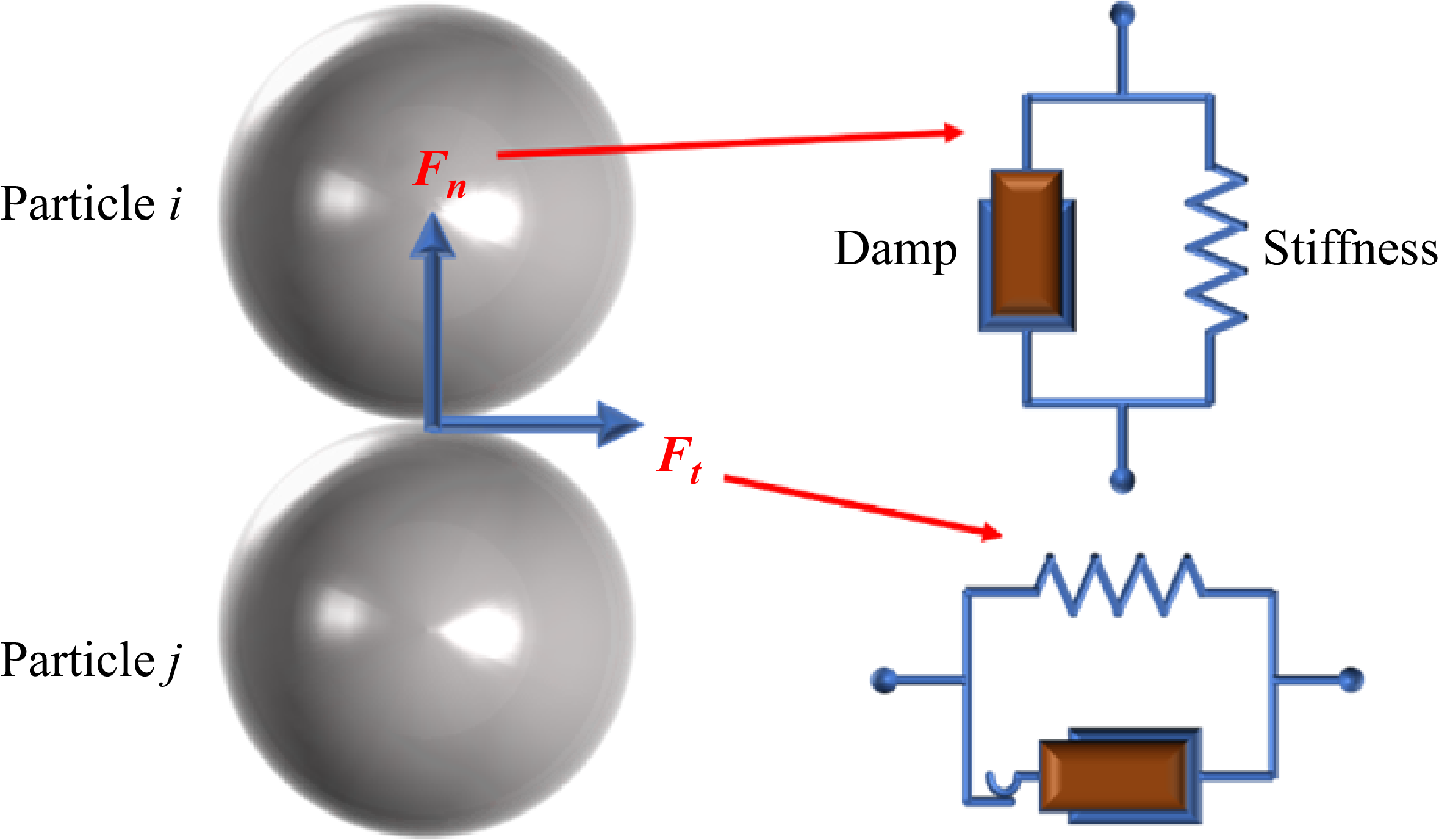
In this study, the modelling of the floating structure is based on discrete element particle clusters established through classical mechanical principles. Within the DEM framework, a soft-sphere contact approach is employed to identify interactions between particles or between particles and solid boundaries. The method accounts for deformations between contacting bodies, which are represented by particle overlaps and subsequently used to compute interparticle forces. The interaction forces are calculated using a nonlinear slip-spring-damper system. The Hertz–Mindlin contact model (Renzo & Maio Reference Renzo and Maio2005) is adopted in this work to characterise the interactions between particles as well as between particles and walls, as shown in figure 1. The collision force between two particles or between a particle and a solid wall can be expressed as
 \begin{equation} F_{c} = F_{n}\boldsymbol{n} + F_{t}\boldsymbol{t}, \end{equation}
where $F_{n}$
and
$F_{n}$
and $F_{t}$
are the normal and tangential components of the contact force, respectively, and the normal force
$F_{t}$
are the normal and tangential components of the contact force, respectively, and the normal force $F_{n}$
can be defined as
$F_{n}$
can be defined as
 \begin{equation} F_{n} = -K_{n}d_{n} - N_{n}v_{n}, \end{equation}
where $K_{n}$
is the normal spring stiffness,
$K_{n}$
is the normal spring stiffness, $d_{n}$
is the normal overlapping distance between particles or between particles and solid wall,
$d_{n}$
is the normal overlapping distance between particles or between particles and solid wall, $N_{n}$
is the normal damping, and
$N_{n}$
is the normal damping, and $v_{n}$
is the normal relative velocity between particles or between particles and solid wall.
$v_{n}$
is the normal relative velocity between particles or between particles and solid wall.

Figure 1. Schematic diagram of particle contact model.
The tangential force can be expressed as
 \begin{equation} \begin{cases} F_{t} = \left |K_{n}d_{n}\right |\!C_{\!{fs}}d_{t}/\!\left |d_{t}\right |, & \quad \left |K_{t}d_{t}\right | \geqslant \left |K_{n}d_{n}\right |\!C_{\!{fs}}, \\ F_{t} = -\!K_{t}d_{t} - N_{t}v_{t}, & \quad \left |K_{t}d_{t}\right | \leqslant \left |K_{n}d_{n}\right |\!C_{\!{fs}}, \end{cases} \end{equation}
where $K_{t}$
is the tangential spring stiffness,
$K_{t}$
is the tangential spring stiffness, $d_{t}$
is the tangential overlapping distance between particles,
$d_{t}$
is the tangential overlapping distance between particles, $v_{t}$
is the tangential relative velocity between particles or between particles and solid wall, and
$v_{t}$
is the tangential relative velocity between particles or between particles and solid wall, and $C_{\!{fs}}$
is the friction coefficient.
$C_{\!{fs}}$
is the friction coefficient.
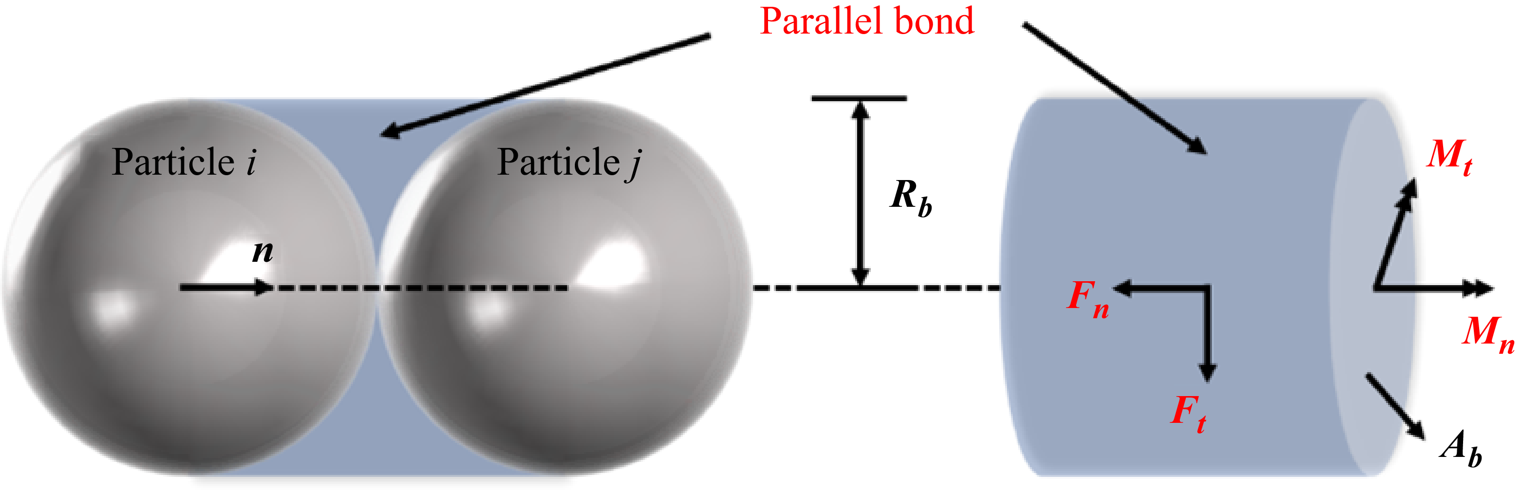
The particle bonding approach enables the extension of discrete particle models to simulate complex geometries and structures. By implementing the parallel bond model to represent mechanical connections between particles, cohesive granular assemblies can be constructed. These assemblies exhibit quasi-continuum elastoplastic mechanical responses when subjected to stresses below the failure threshold (Potyondy & Cundall Reference Potyondy and Cundall2004). Once local stresses exceed the stress limit, the model naturally captures the evolution of crack initiation, bond rupture and fragmented particle behaviour, thereby simulating the complete physical process from intact structure to fragmentation. The parallel bond assumes a bonding disk (or cylinder) with radius $R_b$
centred at the contact point between adjacent particles. The bond radius is typically selected as the smaller radius of the two bonded particles. Forces and moments are transmitted simultaneously through the parallel bond, with normal and tangential forces denoted as
$R_b$
centred at the contact point between adjacent particles. The bond radius is typically selected as the smaller radius of the two bonded particles. Forces and moments are transmitted simultaneously through the parallel bond, with normal and tangential forces denoted as $F_n$
and
$F_n$
and $F_t$
, and normal and tangential moments as
$F_t$
, and normal and tangential moments as $M_n$
and
$M_n$
and $M_t$
, respectively, as shown in figure 2. The tensile stress
$M_t$
, respectively, as shown in figure 2. The tensile stress $\sigma$
(normal bonding strength) and shear stress
$\sigma$
(normal bonding strength) and shear stress $\tau$
(tangential bonding strength) acting on the parallel bond can be expressed as
$\tau$
(tangential bonding strength) acting on the parallel bond can be expressed as
 \begin{align} \sigma &= -\frac {F_n}{A_b} + \frac {\left |M_{t}\right |}{I_b}R_b, \end{align}
 \begin{align} \tau &= \frac {\left |F_t\right |}{A_b} + \frac {\left |M_{n}\right |}{J_b}R_b, \end{align}

Figure 2. Parallel bond between particles.
where $A_b$
is the cross-sectional area of the parallel key,
$A_b$
is the cross-sectional area of the parallel key, $J_b$
is the polar moment of inertia of the parallel key and
$J_b$
is the polar moment of inertia of the parallel key and $I_b$
is the moment of inertia of the parallel key, which can be expressed as
$I_b$
is the moment of inertia of the parallel key, which can be expressed as
 \begin{align} A_b &= \pi\! R_b^2,\\[-12pt]\nonumber \end{align}
 \begin{align} I_b &= \frac {\pi\! R_b^4}{4}, \\[-12pt]\nonumber \end{align}
 \begin{align} J_b &= \frac {\pi\! R_b^4}{2}. \end{align}
When the tensile stress $\sigma$
or shear stress
$\sigma$
or shear stress $\tau$
acting on a parallel bond exceeds its failure strength, the bond will rupture. This bond failure mechanism enables the model to naturally capture crack initiation and damage propagation in the simulated floating ice structure.
$\tau$
acting on a parallel bond exceeds its failure strength, the bond will rupture. This bond failure mechanism enables the model to naturally capture crack initiation and damage propagation in the simulated floating ice structure.
In marine environments, floating structures typically exhibit diverse structural compositions and material properties, with their failure behaviour involving complex mixed-mode fracture mechanisms and energy dissipation pathways (Adamson & Dempsey Reference Adamson and Dempsey1998; Schreyer & Munday Reference Schreyer, Sulsky and Munday2006; Paavilainen & Polojärvi Reference Paavilainen, Tuhkuri and Polojärvi2009; Dempsey & Wang Reference Dempsey, Cole and Wang2018; Lilja & Tuhkuri Reference Liu and Ji2021). However, this study focuses on the transient response during the impact water entry of the projectile, with particular emphasis on how structural damage induced by impact affects subsequent hydrodynamic characteristics. Given that the temporal scope of this investigation focuses on the initial impact and fragmentation phases, a fracture criterion based on interparticle bond failure proves sufficient to capture the essential structural damage features while meeting research requirements. This fracture model maintains computational stability while effectively simulating the transition from intact structures to fragmented particulate states, and their influence on cavity evolution and flow field disturbances. Moreover, it possesses the distinct advantage of characterising structural fragmentation and fracture propagation mechanisms, thereby providing an effective numerical approach for investigating the dynamic response of floating structures subjected to projectile impacts.
2.2. Interaction between fluid and particles
The interaction between the fluid and the dispersed solid phase is described using a locally volume-averaged two-phase formulation within the CFD–DEM framework. The total hydrodynamic force ( $\boldsymbol{f}_{\!i,f}$
) acting on each particle is expressed as the sum of the drag (
$\boldsymbol{f}_{\!i,f}$
) acting on each particle is expressed as the sum of the drag ( $\boldsymbol{f}_{\!d}$
), pressure-gradient (
$\boldsymbol{f}_{\!d}$
), pressure-gradient ( $\boldsymbol{f}_{\kern -3pt p}$
), added-mass (
$\boldsymbol{f}_{\kern -3pt p}$
), added-mass ( $\boldsymbol{f}_{\!a}$
) and buoyancy (
$\boldsymbol{f}_{\!a}$
) and buoyancy ( $\boldsymbol{f}_{\!b}$
) contributions:
$\boldsymbol{f}_{\!b}$
) contributions:
 \begin{align} \boldsymbol{f}_{\!i,f} =\boldsymbol{f}_{\!d}+\boldsymbol{f}_{\kern -3pt p}+\boldsymbol{f}_{\!a}+\boldsymbol{f}_{\!b}, \end{align}
 \begin{align} \boldsymbol{f}_{\!d} = \frac {1}{2} C_{d} A_{\!p} \rho _{\!f} \big ( \boldsymbol{u}_{\!f} - \boldsymbol{u}_{\!p} \big ) \left | \boldsymbol{u}_{\!f} - \boldsymbol{u}_{\!p} \right |\!, \end{align}
where $A_p$
is the projected particle area,
$A_p$
is the projected particle area, $C_d$
is the drag coefficient,
$C_d$
is the drag coefficient, $\boldsymbol{u}_{\!f}$
is the fluid velocity and
$\boldsymbol{u}_{\!f}$
is the fluid velocity and $\boldsymbol{u}_{\!p}$
is the particle velocity.
$\boldsymbol{u}_{\!p}$
is the particle velocity.
The pressure-gradient term accounts for the background flow acceleration:
 \begin{align} \boldsymbol{f}_{\kern -3pt p} = - V_{\!p} \boldsymbol{\nabla }\!p_{\!f}, \end{align}
 \begin{align} \boldsymbol{f}_{\!b} = V_{\!p} (\rho _{\!f} - \rho _{p}) \boldsymbol{g}, \end{align}
where $V_{\!p}$
is the particle volume and
$V_{\!p}$
is the particle volume and $p_{\!f}$
is the local fluid pressure.
$p_{\!f}$
is the local fluid pressure.
The added-mass contribution is included to capture the unsteady acceleration of the surrounding fluid:
 \begin{equation} \boldsymbol{f}_{\!a} = C_{a} V_{\!p} \rho _{\!f} \left ( \frac {{\rm D}\boldsymbol{u}_{\!f}}{{\rm D}t} - \frac {{\rm d}\boldsymbol{u}_{\!p}}{{\rm d}t} \right )\!, \end{equation}
where $C_{a}$
is the virtual mass coefficient.
$C_{a}$
is the virtual mass coefficient.
In computational fluid dynamics, due to the interaction between the gas–liquid interface and particles, the governing equations of the fluid can be written as the volume-averaged continuity and momentum equations:
 \begin{equation} \frac {\partial (\alpha _{\!f} \rho _{\!f})}{\partial t} + \boldsymbol{\nabla }\boldsymbol{\cdot }(\alpha _{\!f} \rho _{\!f} \boldsymbol{u}_{\!f}) = 0, \end{equation}
 \begin{equation} \frac {\partial (\alpha _{\!f} \rho _{\!f} \boldsymbol{u}_{\!f})}{\partial t} +\boldsymbol{\nabla }\boldsymbol{\cdot }(\alpha _{\!f} \rho _{\!f} \boldsymbol{u}_{\!f} \otimes \boldsymbol{u}_{\!f}) = - \alpha _{\!f} \boldsymbol{\nabla }\!p_{\!f} + \boldsymbol{\nabla }\boldsymbol{\cdot }(\alpha _{\!f} \boldsymbol{\tau }_{\!f}) + \alpha _{\!f} \rho _{\!f} \boldsymbol{g} + \boldsymbol{S}_{\!f}, \end{equation}
where $\rho _{\!f}$
is the density of fluid,
$\rho _{\!f}$
is the density of fluid, $\boldsymbol{u}_{\!f}$
is the velocity of the fluid,
$\boldsymbol{u}_{\!f}$
is the velocity of the fluid, $p$
is the pressure,
$p$
is the pressure, $\boldsymbol{\tau }_{\!f}$
is the viscous shear stress tensor,
$\boldsymbol{\tau }_{\!f}$
is the viscous shear stress tensor, $\alpha _{\!f}$
is the volume fraction of the fluid in a single fluid unit (fluid porosity), using the assumption of local average (Tsuji, Kawaguchi & Tanaka Reference Tsuji, Kawaguchi and Tanaka1993), and
$\alpha _{\!f}$
is the volume fraction of the fluid in a single fluid unit (fluid porosity), using the assumption of local average (Tsuji, Kawaguchi & Tanaka Reference Tsuji, Kawaguchi and Tanaka1993), and $S_{\!f}$
is the source term after volume correction (Du et al. Reference Du, Bao, Xu and Wei2006).
$S_{\!f}$
is the source term after volume correction (Du et al. Reference Du, Bao, Xu and Wei2006).
To account for the multiphase media, the volume of fluid (VOF) method is employed to track interfaces between immiscible fluids. In this approach, different fluid phases share a single set of momentum equations, while their interfaces are captured by solving transport equations for volume fraction variables assigned to each phase. The fundamental constraint requires the sum of volume fractions in each computational cell to equal 1. Among them, the density and viscosity of the fluid are weighted and averaged according to the phase fraction, that is, $\rho _{\!f} = \alpha _1 \rho _1 + \alpha _2 \rho _2, \mu _{\!f} = \alpha _1 \mu _1 + \alpha _2 \mu _2$
, where the subscripts 1 and 2 represent the liquid phase and the gas phase, respectively. In the VOF framework, the transport equation of the liquid phase is given as
$\rho _{\!f} = \alpha _1 \rho _1 + \alpha _2 \rho _2, \mu _{\!f} = \alpha _1 \mu _1 + \alpha _2 \mu _2$
, where the subscripts 1 and 2 represent the liquid phase and the gas phase, respectively. In the VOF framework, the transport equation of the liquid phase is given as
 \begin{equation} \frac {\partial (\alpha _1)}{\partial t} + \boldsymbol{\nabla }\boldsymbol{\cdot }(\alpha _1 \boldsymbol{u}_{\!f}) + \boldsymbol{\nabla }\boldsymbol{\cdot }\left [ \alpha _1 (1 - \alpha _1) \boldsymbol{u}_r \right ] = 0, \end{equation}
where $\boldsymbol{u}_r$
is the compression velocity, which is an artificially applied relative velocity field designed to compress the VOF interface and thereby reduce numerical diffusion.
$\boldsymbol{u}_r$
is the compression velocity, which is an artificially applied relative velocity field designed to compress the VOF interface and thereby reduce numerical diffusion.
The first two terms in (2.18) have the same advection form as the volume-fraction form of the continuity equation, indicating that for an incompressible fluid, mass conservation is equivalent to volume conservation; therefore, a volume-fraction variable is introduced. The presence of $\alpha _{\!f}$
in these two terms arises from the local averaging procedure, while
$\alpha _{\!f}$
in these two terms arises from the local averaging procedure, while $\alpha _1$
serves as an indicator of wet/dry conditions. Within the computational domain, a control volume with
$\alpha _1$
serves as an indicator of wet/dry conditions. Within the computational domain, a control volume with $\alpha _1 = 1$
is fully occupied by liquid, whereas a control volume with
$\alpha _1 = 1$
is fully occupied by liquid, whereas a control volume with $\alpha _1 = 0$
corresponds to a dry air region.
$\alpha _1 = 0$
corresponds to a dry air region.
For three-phase flow (gas–liquid–particle), the volume fraction of each phase is shown in figure 3. For three-phase flow, the fluid volume fraction can be expressed as
 \begin{equation} \alpha _{\!f} = 1 - \sum V_{\textit{pi}}/{V_{t}} = (V_{1} + V_{2})/{V_{t}}, \end{equation}
where $V_{\textit{pi}}$
is the volume of the
$V_{\textit{pi}}$
is the volume of the $i$
particle mapped from the particle domain to the corresponding fluid cell,
$i$
particle mapped from the particle domain to the corresponding fluid cell, $V_{1}$
and
$V_{1}$
and $V_{2}$
are the volumes of the liquid phase and gas phase, respectively, and
$V_{2}$
are the volumes of the liquid phase and gas phase, respectively, and $V_{t}$
is the total volume of the cell. While
$V_{t}$
is the total volume of the cell. While $\alpha _{1}$
and
$\alpha _{1}$
and $\alpha _{2}$
can be expressed as the volume fractions of their respective volume ratios (
$\alpha _{2}$
can be expressed as the volume fractions of their respective volume ratios ( $V_{\!f} = V_{1} + V_{2}$
), which can be expressed as
$V_{\!f} = V_{1} + V_{2}$
), which can be expressed as
 \begin{equation} \alpha _{1} = V_{1}/{V_{\!f}}, \end{equation}
 \begin{equation} \alpha _{2} = V_{2}/{V_{\!f}} = 1 - \alpha _{1}. \end{equation}

Figure 3. Volume distribution of the gas–liquid–particle three-phase of the VOF method.
Therefore, the local average phase fraction $\alpha _{\!f}\alpha _{1} = V_{1}/{V_{t}}$
is calculated based on the total volume
$\alpha _{\!f}\alpha _{1} = V_{1}/{V_{t}}$
is calculated based on the total volume $V_{t}$
, which represents the transportation volume as described in (2.20).
$V_{t}$
, which represents the transportation volume as described in (2.20).
The fluid–structure interaction computation is initiated by calculating the fluid porosity in each computational cell based on particle positions and fluid grid information. Subsequently, the fluid–particle interaction forces acting on each particle are determined using particle velocities, fluid velocities and the pressure/stress tensor at the current fluid time step. The Newtonian framework, combined with a drag model, computes the particle–fluid interaction forces within each fluid cell. A sub-cycling DEM time-stepping scheme is then implemented, where particle positions and velocities are updated through explicit integration of Newton’s equations using smaller time increments within each CFD time step. The fluid phase’s mass and momentum conservation equations are solved using the computed porosity and volumetric fluid–particle interaction forces in each cell. The PISO (pressure implicit with splitting of operators) algorithm is employed for solving the fluid equations, with the QUICK (quadratic upstream interpolation for convective kinematics) scheme adopted for discretising convective terms. Gradient and divergence terms are evaluated using a second-order finite difference approach. Numerical stability is governed by the Courant number (Co), which determines the maximum allowable time step. To ensure computational stability, the fluid motion within any grid cell must not exceed a characteristic length per time step, necessitating the use of a fraction of the critical time step for stable temporal integration. The coupling frequency between CFD and DEM domains is determined by the ratio of their respective time steps. Figure 4 presents the complete workflow of this coupling procedure.

Figure 4. Flow chart of fluid–particle interaction.
2.3. Dual-grid method
During grid division, local flow characteristics and resolution requirements must be considered. When projectiles interact with floating structures composed of discrete particles, the relationship between particle size and local fluid grid resolution becomes critical for ensuring both solution accuracy and numerical stability in coupled simulations. To properly capture particle–solid and particle–fluid interaction behaviours, it is generally recommended that particle dimensions should not exceed the scale of local fluid grid cells (Jiang et al. Reference Jiang, Guo, Yu, Hua, Lin, Wassgren and Curtis2021; Cui et al. Reference Cui, Harris, Howarth, Zealey, Brown and Shepherd2022; Mathews et al. Reference Mathews, Khan, Sharma, Kumar and Kumar2022; Zhu et al. Reference Zhu, He, Zhao, Vowinckel and Meiburg2022). However, when dealing with relatively large particles, coarser grids may be employed in surrounding regions to reduce computational costs, which may reduce the resolution of local flow details. In the present study, a balanced approach is adopted to maintain computational efficiency and the analysability of fragmented structures. The particle size is deliberately maintained above a minimum threshold to guarantee that post-impact floating structures develop representative particulate configurations with observable dynamic responses. Simultaneously, the water entry process of the projectile involves complex gas–liquid interface deformation and cavity evolution phenomena, necessitating refined grids for accurate interface dynamics resolution. This inherent conflict between particle-scale requirements and fluid grid refinement creates fundamental challenges in simultaneously satisfying the resolution needs of both physical processes within a single grid system.
To address the scale disparity between particle dimensions and fluid grid resolution, this study introduces a dual-grid methodology. The approach employs a nested coarse–fine grid structure that facilitates bidirectional information transfer between particles and fluids, significantly enhancing simulation efficiency while maintaining physical consistency. The schematic diagram of the dual-grid algorithm is shown in figure 5. Based on classical volume-averaging theory, the method first processes particle distributions on the coarse grid to construct a spatially continuous particle-phase field. This field estimates local porosity, drag source terms and particle-induced momentum transport effects. This process can be regarded as a reverse interpolation operation that projects discrete Lagrangian particle data onto an Eulerian coarse-grid framework for coupling term computation. Following the derivation of averaged particle-phase variables on the coarse scale, the coupling information is subsequently mapped onto the fine-scale fluid resolution grid to capture local flow features such as free-surface deformation and cavity boundaries. The fluid governing equations are solved within this support domain, with initial conditions provided by the coarse-scale averaged field. The projection of Lagrangian variables ensures source-term consistency at the averaging scale, while the support-domain grid can be adaptively refined based on local flow requirements, typically independent of particle distribution characteristics. Upon obtaining the fine-scale fluid solutions, these results are back-projected to update the coarse-grid averaged field, completing an information feedback loop that enables efficient multiscale, multiphysics interaction and dynamic synchronisation between particles and fluids.

Figure 5. A cluster group of continuous grid elements coupled by the dual-grid method. Larger grid elements are used to calculate the interaction between the particle beam and the liquid phase. Refined grid elements are then employed to solve the fluid equations. Upon the interaction calculation, the simulation distributes the effects of volume fraction, momentum, energy source terms and other transport quantities across the component grid elements.
Based on the aforementioned dual-grid coupling framework, this study employs a three-dimensional bilinear interpolation scheme for information transfer between coarse grids ( $\varOmega _{c}$
) and fine grids (
$\varOmega _{c}$
) and fine grids ( $\varOmega _{k}$
), ensuring accurate mapping of physical quantities across different grid scales. To maintain interpolation accuracy and numerical consistency, the fluid domain is discretised using structured hexahedral grids. For each fine-grid node, the interpolation references data from the eight vertex nodes of its encompassing coarse-grid cell, as illustrated in figure 6. Specifically, a given fine-grid node is located within a coarse cell defined by eight vertices with spatial coordinates
$\varOmega _{k}$
), ensuring accurate mapping of physical quantities across different grid scales. To maintain interpolation accuracy and numerical consistency, the fluid domain is discretised using structured hexahedral grids. For each fine-grid node, the interpolation references data from the eight vertex nodes of its encompassing coarse-grid cell, as illustrated in figure 6. Specifically, a given fine-grid node is located within a coarse cell defined by eight vertices with spatial coordinates $(x_{i}, y_{i}, z_{i})$
and
$(x_{i}, y_{i}, z_{i})$
and $i=1$
–8. These vertices correspond to physical variable values
$i=1$
–8. These vertices correspond to physical variable values $\varphi _{\textit{coarse}}(x_{i},y_{i},z_{i})$
on the coarse grid. The interpolated value at the fine-grid node is computed through a weighted average, in which the contribution of each coarse grid vertex is determined according to the distance weight
$\varphi _{\textit{coarse}}(x_{i},y_{i},z_{i})$
on the coarse grid. The interpolated value at the fine-grid node is computed through a weighted average, in which the contribution of each coarse grid vertex is determined according to the distance weight $w_{i}$
, which effectively reflects the spatial influence of coarse grid vertices on fine-grid nodes. However, for fine-grid nodes positioned on the interface between two or more adjacent coarse cells, a multi-cell weighted averaging method is adopted to guarantee the continuity of the field across coarse-cell boundaries. The fine-scale quantity is computed as
$w_{i}$
, which effectively reflects the spatial influence of coarse grid vertices on fine-grid nodes. However, for fine-grid nodes positioned on the interface between two or more adjacent coarse cells, a multi-cell weighted averaging method is adopted to guarantee the continuity of the field across coarse-cell boundaries. The fine-scale quantity is computed as
 \begin{equation} \varphi _{\textit{fine}}(x,y,z) = \frac {\sum _{i=1}^{N_c} w_i \varphi _{\textit{coarse}}(x_i,y_i,z_i)}{\sum _{i=1}^{N_c} w_i}, \end{equation}
 \begin{equation} w_i = \frac {1}{| \boldsymbol{r}_{\!f} - \boldsymbol{r}_c |^n}, \end{equation}

Figure 6. Interpolation processing of grid nodes in the dual-grid method.
where $N_c$
denotes the number of adjacent coarse grids,
$N_c$
denotes the number of adjacent coarse grids, $ \boldsymbol{r}_{\!f}$
and
$ \boldsymbol{r}_{\!f}$
and $ \boldsymbol{r}_c$
denote the position vectors of the fine-node and coarse-grid centres, respectively, and
$ \boldsymbol{r}_c$
denote the position vectors of the fine-node and coarse-grid centres, respectively, and $ n$
is a weighting exponent. The value of
$ n$
is a weighting exponent. The value of $ n$
is 2 (weighted by inverse distance square), which is based on its balance between locality and smoothness, and is consistent with the commonly used spatial interpolation methods.
$ n$
is 2 (weighted by inverse distance square), which is based on its balance between locality and smoothness, and is consistent with the commonly used spatial interpolation methods.
Through the aforementioned weighted averaging procedure, physical variables at fine-grid nodes can be derived from the values at the eight vertex nodes of their encompassing coarse-grid cell. The interpolation process involves two key steps: first, determining the position of the target fine-grid node within the coarse grid (i.e. identifying its host coarse cell); second, extracting the spatial coordinates $(x_{i}, y_{i}, z_{i})$
and corresponding variable values
$(x_{i}, y_{i}, z_{i})$
and corresponding variable values $\varphi _{\textit{coarse}}(x_{i}, y_{i}, z_{i})$
from these eight vertices to compute the interpolation weights
$\varphi _{\textit{coarse}}(x_{i}, y_{i}, z_{i})$
from these eight vertices to compute the interpolation weights $w_{i}$
, ultimately yielding the fine-grid nodal value
$w_{i}$
, ultimately yielding the fine-grid nodal value $\varphi _{\textit{fine}}(x,y,z)$
.
$\varphi _{\textit{fine}}(x,y,z)$
.
To achieve bidirectional information transfer between fine and coarse grids, the fluid variables obtained from fine-grid computations must be projected back onto the coarse grid to update the averaged field at the coarse scale. This coarsening procedure is implemented through a control-volume weighted averaging approach. The average physical quantity $\overline {\varphi }_{\textit{coarse}}$
on each coarse grid (
$\overline {\varphi }_{\textit{coarse}}$
on each coarse grid ( $\varOmega _{c}$
) is calculated. This is determined by collecting the contributions of all fine grids (
$\varOmega _{c}$
) is calculated. This is determined by collecting the contributions of all fine grids ( $\varOmega _{\!f}$
),
$\varOmega _{\!f}$
),
 \begin{equation} \overline {\varphi }_{\textit{coarse}} = \frac {\sum _{\varOmega _{c}}\! \varphi _{\textit{fine}}\! V_{\textit{fine}}}{\sum _{\varOmega _{c}}\! V_{\textit{fine}}}, \end{equation}
where $\overline {\varphi }_{\textit{coarse}}$
is the average physical quantity on each coarse grid and
$\overline {\varphi }_{\textit{coarse}}$
is the average physical quantity on each coarse grid and $V_{\textit{fine}}$
is the volume of the fine grid. For a given coarse grid node, its value is determined by the central value
$V_{\textit{fine}}$
is the volume of the fine grid. For a given coarse grid node, its value is determined by the central value $\overline {\varphi }_{\textit{coarse}}$
of all adjacent coarse grids sharing the node:
$\overline {\varphi }_{\textit{coarse}}$
of all adjacent coarse grids sharing the node:
 \begin{equation} \varphi _{\textit{coarse}}(x_{i}, y_{i}, z_{i}) = \frac {\sum _{N_{c}}\! w_{i} \overline {\varphi }_{\textit{coarse}}}{\sum _{N_{c}}\! w_{i}}. \end{equation}
Note that (2.25) reconstructs coarse-grid nodal values from cell-centred averages for use in the next interpolation step (2.23). While the inverse-distance weighting does not guarantee exact reversibility between nodal and cell-centred values, global conservation is maintained via the volume-weighted averaging in (2.24) after each fine-grid solution, because the sum of fine-grid fluxes over a coarse cell equals the coarse-cell flux. To minimise artificial diffusion of sharp gradients, the fine grid is concentrated in regions of high flow activity (impact zone, cavity interface) and a gradient-limited interpolation is employed when mapping from coarse to fine grids. The method has been validated on benchmark problems with steep gradients and shows negligible loss of local accuracy for the present impact water entry simulations.
The dual-grid system, through the aforementioned interpolation and weighted-averaging procedures, establishes bidirectional variable transfer between coarse- and fine-scale grids, ensuring effective coupling between particulate and fluid phases while demonstrating remarkable precision preservation in high-resolution computational domains. This methodology constructs averaged fields on coarse grids to reduce computational expense, while simultaneously resolving local fluid dynamics through fine-scale meshing, thereby maintaining global numerical stability without compromising local accuracy. By synergistically combining volume-averaging theory with multipoint interpolation techniques, the approach provides a robust and efficient solution strategy for multiscale multiphase flow problems, particularly well suited for numerical simulations involving complex boundary deformation, particle fragmentation and strong fluid–structure interactions.
3. Numerical validation and discussion
This section begins by establishing the physical model, followed by grid generation for both fluid and solid domains, and concludes with systematic validation of the coupling algorithm. Given the study’s focus on multiphase fluid–structure interaction coupled with dual-grid methodology, the verification protocol employs a comprehensive analytical approach. The validation procedure first examines a canonical free water-entry case through numerical simulation to evaluate grid strategy appropriateness, thereby determining the minimum required fluid grid resolution for specific scenarios. This grid-scale analysis provides theoretical and numerical foundations for subsequent discrete element method particle size selection. Following the establishment of an optimal grid framework, floating structure modelling proceeds with corresponding particle parameters. The methodology’s validity is further verified through laboratory experiments comparing numerical simulations against data during impact water entry. This multi-stage validation ensures the proposed approach maintains accuracy and reliability when handling complex fluid–structure interactions and multiscale coupling phenomena. Two distinct numerical experiments are performed to systematically verify different aspects of the methodology.
-
(i) Free water-entry simulation: this case, without floating ice, serves to establish grid-independence and determine the appropriate fluid-grid resolution, thereby providing a baseline for the fluid solver and grid-strategy validation.
-
(ii) Impact water entry simulation with floating ice: this case includes the full fluid–structure–particle coupling. It is validated against laboratory experiments to confirm the accuracy of the DEM particle parameters, the ice-failure model and the overall coupled algorithm under realistic impact conditions.
Both experiments share the same projectile geometry, material properties and fluid-solver settings, allowing a focused assessment of the added complexity introduced by the floating structure and the discrete-element representation.
3.1. Physical model
Under the CFD–DEM dual-grid algorithm framework, a physical model for the impact water entry of a projectile is established, as shown in figure 7. The dimensions of the projectile are scaled based on the currently employed marine detectors (Li et al. Reference Li, Sun, Yao, Wang and Li2020; Jiang et al. Reference Jiang, Guo, Yu, Hua, Lin, Wassgren and Curtis2021; Hu, Wei & Wang Reference Hu, Wei and Wang2023) and modelled as a rigid body, featuring a conical-nosed cylindrical geometry with a diameter of $D_{0} = 0.016\,\text{m}$
, a body length of
$D_{0} = 0.016\,\text{m}$
, a body length of $L_{\!p} = 3.375D_{0}$
, a nose cone angle of
$L_{\!p} = 3.375D_{0}$
, a nose cone angle of $\theta = 120^\circ$
(the conical head is processed by arc and the radius of arc is 0.0008 m) and a cross-sectional area of
$\theta = 120^\circ$
(the conical head is processed by arc and the radius of arc is 0.0008 m) and a cross-sectional area of $S_{p} = \pi (D_{0})^{2}/4$
. The projectile is constructed from aluminium with a density of
$S_{p} = \pi (D_{0})^{2}/4$
. The projectile is constructed from aluminium with a density of $\rho _{p} = 2700\,\text{kg}\,\text{m}^{-3}$
, an elastic modulus of
$\rho _{p} = 2700\,\text{kg}\,\text{m}^{-3}$
, an elastic modulus of $E_{\!p} = 27\,\text{GPa}$
and a strength of
$E_{\!p} = 27\,\text{GPa}$
and a strength of $150\,\text{MPa}$
. The computational domain measured
$150\,\text{MPa}$
. The computational domain measured $L_{\!f} \times W_{\!f} \times H_{\!f} = 20D_{0} \times 20D_{0} \times 42D_{0}$
, with a water depth of
$L_{\!f} \times W_{\!f} \times H_{\!f} = 20D_{0} \times 20D_{0} \times 42D_{0}$
, with a water depth of $H_{w} = 32D_{0}$
. Pressure outlet boundary conditions are imposed on the domain boundaries. The density and viscosity of water are
$H_{w} = 32D_{0}$
. Pressure outlet boundary conditions are imposed on the domain boundaries. The density and viscosity of water are $\rho _{1} = 1000\,\text{kg}\,\text{m}^{-3}$
and
$\rho _{1} = 1000\,\text{kg}\,\text{m}^{-3}$
and $\mu _{1} = 0.00179\,\text{Pa}\boldsymbol{\cdot }\text{s}$
, while the density and viscosity of air are
$\mu _{1} = 0.00179\,\text{Pa}\boldsymbol{\cdot }\text{s}$
, while the density and viscosity of air are $\rho _{2} = 1.294\,\text{kg}\,\text{m}^{-3}$
and
$\rho _{2} = 1.294\,\text{kg}\,\text{m}^{-3}$
and $\mu _{2} = 0.000017\,\text{Pa}\boldsymbol{\cdot }\text{s}$
, respectively.
$\mu _{2} = 0.000017\,\text{Pa}\boldsymbol{\cdot }\text{s}$
, respectively.

Figure 7. Physical model of impact water entry. The entire domain is divided into three regions: the air domain, the water domain and the particle domain. Air and water form an interface (liquid surface), with the flat ice composed of discrete particles arranged in layers following a hexagonal close-packed structure. The size and physical properties of each particle are uniform.
In marine environments, particularly in polar and high-latitude regions, the free surface is often populated with various floating structures, including floating ice, marine debris and natural drift objects. These floating structures, commonly encountered in polar exploration, marine deployment and underwater operations, constitute a non-negligible pre-existing medium during the water entry process of the projectile. Addressing this practical concern, this study incorporates floating ice as a representative floating structure into the modelling and analysis of impact water entry. In terms of modelling, recent studies have employed DEM to simulate the mechanical response of ice, typically by constructing particle systems with bonding models to reconstruct intact ice structures for numerical analysis of their physical parameters and failure behaviour (Long, Ji & Wang Reference Long, Ji and Wang2019; Pradana & Qian Reference Pradana and Qian2020; Zhang et al. Reference Zhang, Tao, Wang, Ye and Guo2021). Although these investigations have primarily focused on solid mechanics without addressing strong fluid–structure interactions involving fluid, they have established critical modelling foundations for this study, particularly in particle parameter selection and contact model formulation. Within the optimised CFD–DEM coupling framework, floating ice is represented by discrete particle assemblies, where mechanical continuity is maintained through parallel bond models to effectively characterise ice deformation and fracture under impact loading. To balance numerical stability with physical representativeness, the ice dimensions and material parameters are derived from actual polar ice properties, with appropriate geometric and physical scaling based on similarity principles (Yang et al. Reference Yang, Sun, Zhang, Yang and Lubbad2024a ,Reference Yang, Sun, Zhang, Yang and Lubbad b ).
The floating ice is modelled with fundamental dimensions of $L_{l} \times L_{w} \times L_{t} = 12.5D_{0} \times 12.5D_{0} \times 1D_{0}$
, a density of
$L_{l} \times L_{w} \times L_{t} = 12.5D_{0} \times 12.5D_{0} \times 1D_{0}$
, a density of $\rho _{\textit{ice}} = 900\,\text{kg}\,\text{m}^{-3}$
, a bending strength of
$\rho _{\textit{ice}} = 900\,\text{kg}\,\text{m}^{-3}$
, a bending strength of $\sigma _{f,\textit{ice}} = 0.81\,\text{MPa}$
, a compressive strength of
$\sigma _{f,\textit{ice}} = 0.81\,\text{MPa}$
, a compressive strength of $\sigma _{c,\textit{ice}} = 2.56\,\text{MPa}$
and an elastic modulus of
$\sigma _{c,\textit{ice}} = 2.56\,\text{MPa}$
and an elastic modulus of $E_{\textit{ice}} = 0.7\,\text{GPa}$
. From a discrete element perspective, the ice is discretised into elemental particles whose material properties govern the bulk behaviour of the floating ice. The physical parameters of the ice have an adaptive relationship with the particle parameters. The particle-scale parameters set in the numerical simulation are based on the particle-bond mapping framework established by Long et al. (Reference Long, Ji and Wang2019) with a particle density of
$E_{\textit{ice}} = 0.7\,\text{GPa}$
. From a discrete element perspective, the ice is discretised into elemental particles whose material properties govern the bulk behaviour of the floating ice. The physical parameters of the ice have an adaptive relationship with the particle parameters. The particle-scale parameters set in the numerical simulation are based on the particle-bond mapping framework established by Long et al. (Reference Long, Ji and Wang2019) with a particle density of $\rho _{\textit{ip}} = 900\ \text{kg}\,\text{m}^{-3}$
, normal bonding strength of
$\rho _{\textit{ip}} = 900\ \text{kg}\,\text{m}^{-3}$
, normal bonding strength of $\sigma = 1.2\ \mathrm{MPa}$
, tangential bonding strength of
$\sigma = 1.2\ \mathrm{MPa}$
, tangential bonding strength of $\tau = 0.8\ \mathrm{MPa}$
, friction coefficient of
$\tau = 0.8\ \mathrm{MPa}$
, friction coefficient of $C_{\!{fs}} = 0.2$
and elastic modulus of
$C_{\!{fs}} = 0.2$
and elastic modulus of $E_{\textit{ip}} = 0.5\ \mathrm{GPa}$
. A detailed validation of these particle parameter selections will be presented in subsequent sections.
$E_{\textit{ip}} = 0.5\ \mathrm{GPa}$
. A detailed validation of these particle parameter selections will be presented in subsequent sections.
Initially, the ice remains stationary on the liquid level. The velocity of the projectile is denoted as $u_{\!p}$
, with an initial water entry velocity of
$u_{\!p}$
, with an initial water entry velocity of $u_{\!p0} = 20\,\text{m s}^{-1}$
, and the
$u_{\!p0} = 20\,\text{m s}^{-1}$
, and the $\textit{Fr} = u_{\!p0}/\sqrt {\textit{gD}_{0}} = 50$
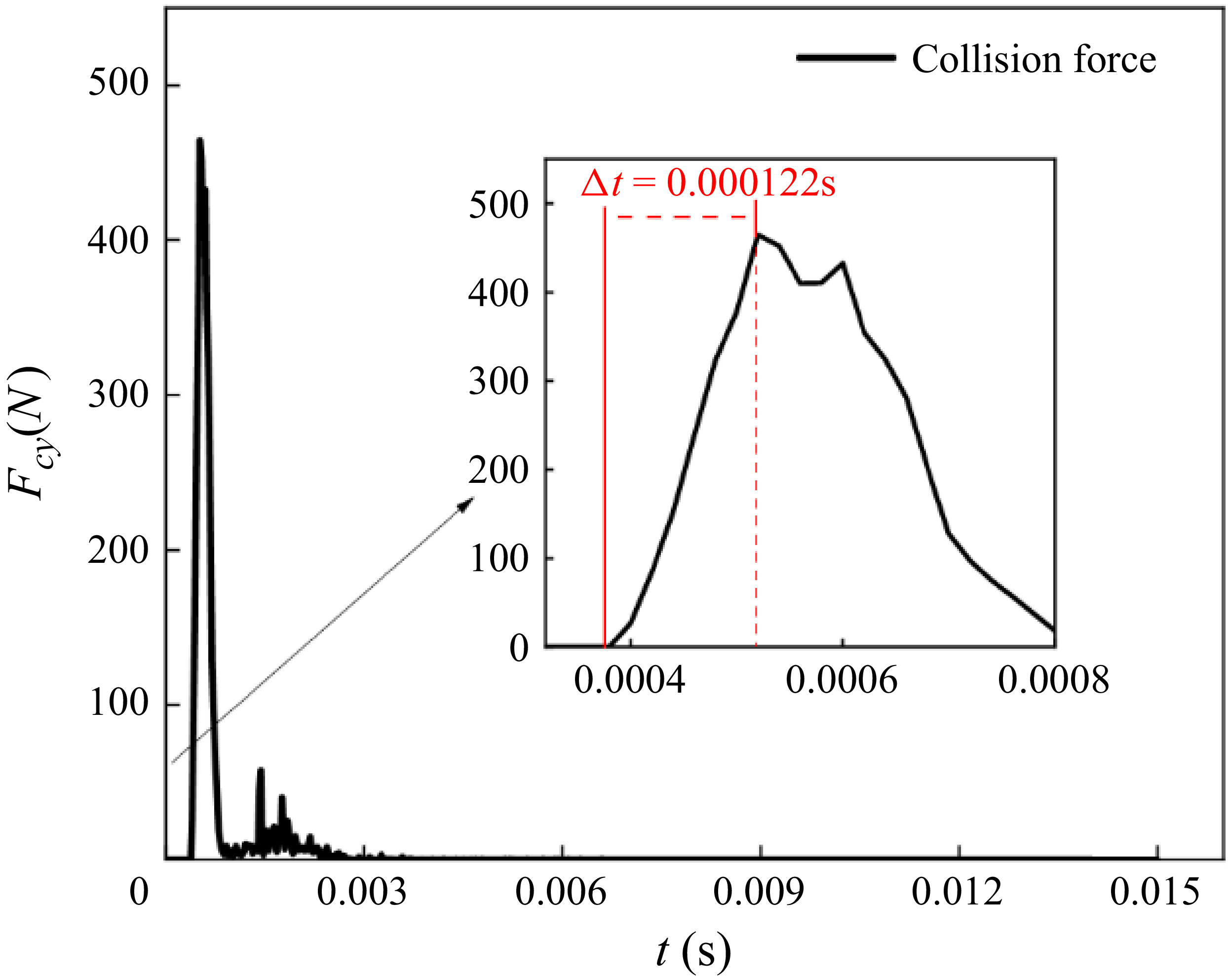
. Characteristic parameters are dimensionless in the numerical simulations, including the hydrodynamic force
$\textit{Fr} = u_{\!p0}/\sqrt {\textit{gD}_{0}} = 50$
. Characteristic parameters are dimensionless in the numerical simulations, including the hydrodynamic force $F_{n}^{*} = F_{h}/0.5\rho _{w}c_{\textit{ice}}^{2}S_{p}$
, collision force
$F_{n}^{*} = F_{h}/0.5\rho _{w}c_{\textit{ice}}^{2}S_{p}$
, collision force $F_{c}^{*} = F_{c}/0.5\rho _{w}c_{\textit{ice}}^{2}S_{p}$
, water entry speed
$F_{c}^{*} = F_{c}/0.5\rho _{w}c_{\textit{ice}}^{2}S_{p}$
, water entry speed $u_{\!p}^{*} = u_{\!p}/c_{\textit{ice}}$
, movement time
$u_{\!p}^{*} = u_{\!p}/c_{\textit{ice}}$
, movement time $t^{*} = t/(D_{0}/c_{\textit{ice}})$
and displacement
$t^{*} = t/(D_{0}/c_{\textit{ice}})$
and displacement $L^{*}_{\textit{pi}} = L_{\textit{pi}} / D_{0}\ (i = x, y, z)$
. Since the impact of the projectile on the floating ice involves stress wave propagation, the characteristic velocity (
$L^{*}_{\textit{pi}} = L_{\textit{pi}} / D_{0}\ (i = x, y, z)$
. Since the impact of the projectile on the floating ice involves stress wave propagation, the characteristic velocity ( $c_{\textit{ice}}$
) used in the dimensionless treatment is defined as the stress wave propagation velocity in ice.
$c_{\textit{ice}}$
) used in the dimensionless treatment is defined as the stress wave propagation velocity in ice.
3.2. Numerical method verification
The fluid domain is discretised using structured hexahedral grids, as shown in figure 8, to balance computational efficiency with the data mapping regularity between coarse and fine grids in the dual-grid framework. This grid topology offers superior alignment consistency and controllable resolution, thereby enhancing both coupling efficiency and convergence stability in the numerical simulations.

Figure 8. Grid division of the fluid domain.
To maintain numerical stability during time advancement, the Courant number ( $Co = U\!\Delta t/\Delta x$
, where
$Co = U\!\Delta t/\Delta x$
, where $U\!\Delta t$
represents the fluid flow distance and
$U\!\Delta t$
represents the fluid flow distance and $\Delta x$
is the grid length) must be maintained below 1. The grid resolution is characterised by
$\Delta x$
is the grid length) must be maintained below 1. The grid resolution is characterised by $D_{0}/\Delta x$
, where
$D_{0}/\Delta x$
, where $D_{0}$
serves as the characteristic length scale.
$D_{0}$
serves as the characteristic length scale.
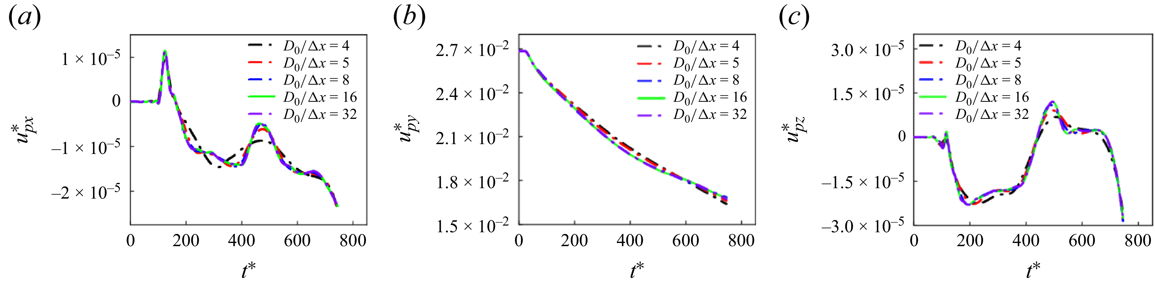
To evaluate the rationality of the fluid domain meshing strategy and ensure numerical convergence, a grid-independence study is conducted using a canonical free water-entry case. This case is selected because it employs exactly the same fluid solver settings, boundary conditions, free-surface treatment and grid generation strategy as the ice-breaking water entry simulations, while avoiding DEM coupling. The absence of discrete elements substantially reduces the computational cost, allowing a more systematic assessment of mesh refinement effects under identical fluid conditions and ensuring that the selected mesh resolution is both physically accurate and computationally efficient. During validation, the background grid size is systematically adjusted in the vicinity of the projectile and along its water entry trajectory, with primary focus on analysing the convergence behaviour of the body’s velocity response under different grid resolutions. Figure 9 illustrates the velocity variations during the impact water entry for various grid resolutions. The numerical results demonstrate that as grid refinement progresses, the velocity components in all directions exhibit convergent behaviour, indicating satisfactory grid independence. Balancing numerical accuracy with computational cost, a grid resolution of $D_{0}/\Delta x=16$
is selected for this study, corresponding to a minimum grid size of 0.001 m near the free surface. This configuration adequately satisfies the resolution requirements for both free surface tracking and cavity interface capture.
$D_{0}/\Delta x=16$
is selected for this study, corresponding to a minimum grid size of 0.001 m near the free surface. This configuration adequately satisfies the resolution requirements for both free surface tracking and cavity interface capture.

Figure 9. Velocity of the projectile during water entry under different grid resolutions. The free water-entry condition maintains consistency with the impact water entry, $\textit{Fr}=50$
. Velocity components along the
$\textit{Fr}=50$
. Velocity components along the $x$
,
$x$
, $y$
and
$y$
and $z$
axes of the Cartesian coordinate system are obtained to characterise the directional velocity distributions.
$z$
axes of the Cartesian coordinate system are obtained to characterise the directional velocity distributions.
To validate the numerical accuracy and physical reliability of the CFD–DEM coupling framework with the dual-grid method, a laboratory experiment of impact water entry is designed, as shown in figure 10. The experiment is performed in a $1.5\,\text{m} \times 0.8\,\text{m} \times 0.9\,\text{m}$
glass water tank maintained at low ambient temperature to effectively retard ice phase transition processes.
$1.5\,\text{m} \times 0.8\,\text{m} \times 0.9\,\text{m}$
glass water tank maintained at low ambient temperature to effectively retard ice phase transition processes.

Figure 10. Experimental device for impact water entry: (a) schematic diagram of the experiment; (b) experimental equipment.
The projectile is launched using a pneumatic ejection system, where the gas filling volume is controlled through a preset air pressure and instantaneously released via an electromagnetic valve. The gas content is adjusted to achieve an initial impact velocity of $u_{\!p0} = 20\,\text{m}\,\rm s^{-1}$
, with the projectile’s geometric dimensions and material parameters maintained consistent with those specified in § 3. The water entry process is captured using a FASTCAM SA-5 high-speed imaging system operating at 1500 fps to ensure sufficient temporal resolution for the dynamic process. A 50 W directional LED light source, positioned behind the water tank and coupled with a flexible diffuser screen, provides uniform backlight illumination to minimise measurement errors caused by interfacial refraction. The spatial relationships among the camera, light source and water surface are calibrated to maintain stable focus in the imaging area and ensure clear visualisation of the water entry cavity. Synchronisation between the launching device and imaging system is achieved through a central control computer.
$u_{\!p0} = 20\,\text{m}\,\rm s^{-1}$
, with the projectile’s geometric dimensions and material parameters maintained consistent with those specified in § 3. The water entry process is captured using a FASTCAM SA-5 high-speed imaging system operating at 1500 fps to ensure sufficient temporal resolution for the dynamic process. A 50 W directional LED light source, positioned behind the water tank and coupled with a flexible diffuser screen, provides uniform backlight illumination to minimise measurement errors caused by interfacial refraction. The spatial relationships among the camera, light source and water surface are calibrated to maintain stable focus in the imaging area and ensure clear visualisation of the water entry cavity. Synchronisation between the launching device and imaging system is achieved through a central control computer.
The ice specimens used in the experiment are prepared by the artificial freezing method to ensure their geometric consistency and physical controllability. The ice specimens used for impact water entry experiments have standardised dimensions of $L_l \times L_w \times L_t = 12.5D_0 \times 12.5D_0 \times 1D_0$
, with a density of
$L_l \times L_w \times L_t = 12.5D_0 \times 12.5D_0 \times 1D_0$
, with a density of $\rho _{\textit{ice}} = 900\,\text{kg}\,\text{m}^{-3}$
, a bending strength of
$\rho _{\textit{ice}} = 900\,\text{kg}\,\text{m}^{-3}$
, a bending strength of $\sigma _{f,\textit{ice}} = 0.81\,\text{MPa}$
, a compression strength of
$\sigma _{f,\textit{ice}} = 0.81\,\text{MPa}$
, a compression strength of $\sigma _{c,\textit{ice}} = 2.56\,\text{MPa}$
and an elastic modulus of
$\sigma _{c,\textit{ice}} = 2.56\,\text{MPa}$
and an elastic modulus of $E_{\textit{ice}} = 0.7\,\text{GPa}$
. Before impact water entry, each ice specimen is positioned to float freely on the water surface with its geometric centre precisely aligned with the rotational axis of the projectile, ensuring ideal axisymmetric normal impact conditions. The initial water entry velocity is set to
$E_{\textit{ice}} = 0.7\,\text{GPa}$
. Before impact water entry, each ice specimen is positioned to float freely on the water surface with its geometric centre precisely aligned with the rotational axis of the projectile, ensuring ideal axisymmetric normal impact conditions. The initial water entry velocity is set to $u_p = 20\,\text{m}\,\text{s}^{-1}$
.
$u_p = 20\,\text{m}\,\text{s}^{-1}$
.
Numerical simulations maintained identical geometric parameters and initial motion conditions for the projectile as specified in § 3, with particular attention given to the construction of the floating ice model at the free surface. The ice’s dimensions and material properties correspond to the experimental conditions, where the thickness $L_t = 1D_0$
, the number of particle layers is 8 for ice thickness (the total number of particles is 63 744) and the corresponding single particle size is
$L_t = 1D_0$
, the number of particle layers is 8 for ice thickness (the total number of particles is 63 744) and the corresponding single particle size is $D_{\textit{ip}} = 0.0024\,\text{m}$
, based on the particle size calculation method in the supplementary material available at https://doi.org/10.1017/jfm.2026.11203. In the optimal grid strategy adopted in the fluid domain, the minimum grid size of the background area is
$D_{\textit{ip}} = 0.0024\,\text{m}$
, based on the particle size calculation method in the supplementary material available at https://doi.org/10.1017/jfm.2026.11203. In the optimal grid strategy adopted in the fluid domain, the minimum grid size of the background area is $0.001\,\text{m}$
, which is smaller than the size of particles, so the dual-grid method is adopted to resolve the matching problem between the fluid grid and the particle size.
$0.001\,\text{m}$
, which is smaller than the size of particles, so the dual-grid method is adopted to resolve the matching problem between the fluid grid and the particle size.
A systematic comparative analysis is conducted between numerical simulations and experimental results of impact water entry. Figure 11 presents the dynamic responses during the impact process, including cavity evolution, velocity and displacement. The simulation results obtained using the dual-grid optimised CFD–DEM algorithm demonstrate agreement with experimental data in terms of trajectory, velocity drop characteristics and overall water entry behaviour. The numerical simulations exhibit certain discrepancies with experimental results in terms of the quantity and morphology of floating ice fragments generated during impact-induced breakage. These differences primarily stem from the inherent randomness of ice fracture processes and the simplified treatment of particle geometry in discrete element modelling. Nevertheless, the numerical approach effectively captures the overall motion characteristics and spatial distribution patterns of the fragments, demonstrating that the proposed coupling method possesses strong physical representational capabilities for modelling dynamic fracture processes. Comparative analysis with conventional grid simulations reveals that the absence of dual-grid refinement leads to symmetric cavity structures after impact, failing to reproduce the cavity fragmentation and collapse observed experimentally due to insufficient particle–fluid coupling. Both experimental observations and dual-grid simulations demonstrate that cavity development is significantly influenced by ice fragments, resulting in irregular boundaries and discontinuous cavity structures. This highlights the critical role of fractured particles in the coupled body–ice–fluid system. Conventional CFD–DEM approaches with unmatched grid scales fail to adequately resolve two-way fluid–particle interactions, which significantly undermines the accuracy of cavity evolution and the flow field.

Figure 11. Comparison between numerical simulations and experimental results ( $\textit{Fr}=50$
, size of ice
$\textit{Fr}=50$
, size of ice $L_{l} \times L_{v} \times L_{\!f} = 12.5D_{0} \times 12.5D_{0} \times 1D_{0}$
). (a) Experimental results of the impact water entry process. (b) Numerical simulation results of the impact water entry process with the dual-grid method. (c) Numerical simulation results of the impact water entry process without the dual-grid method. (d) Comparison of dimensionless vertical velocity components during the impact water entry process. (e) Comparison of dimensionless vertical displacement components during the impact water entry process. Panels (a)–(c) show front views (
$L_{l} \times L_{v} \times L_{\!f} = 12.5D_{0} \times 12.5D_{0} \times 1D_{0}$
). (a) Experimental results of the impact water entry process. (b) Numerical simulation results of the impact water entry process with the dual-grid method. (c) Numerical simulation results of the impact water entry process without the dual-grid method. (d) Comparison of dimensionless vertical velocity components during the impact water entry process. (e) Comparison of dimensionless vertical displacement components during the impact water entry process. Panels (a)–(c) show front views ( $x$
–
$x$
– $y$
plane observations). In panels (b) and (c), upper parts show global impact processes while lower parts display cavity evolution by hiding particle phases.
$y$
plane observations). In panels (b) and (c), upper parts show global impact processes while lower parts display cavity evolution by hiding particle phases.
To further evaluate the differences in ice structure damage evolution and broken ice particle dynamics under different algorithms, this study conducted a comparative analysis of the failure patterns and particle motion characteristics of floating ice during impact water entry, as shown in figure 12. In the experiment, a flexible capture net is installed at the tank bottom to capture fragmented ice pieces, which are subsequently retrieved and reconstructed immediately after each test to examine final fracture morphology. Figure 12(a) presents the observed ice failure modes. When employing the dual-grid method, despite minor discrepancies in fracture locations compared with experimental results, considering inevitable experimental disturbances (such as temperature gradients, water surface fluctuation, etc.), the simulations successfully reproduced the primary crack propagation paths and their topological features, with fracture counts matching experimental observations. In contrast, simulations without dual-grid refinement exhibited more branched cracks and premature structural failure, along with significantly enhanced particle dispersion phenomena at both the ice–fluid interface and the lower surface of the penetration zone. These observations are corroborated by figures 11(c) and 13, demonstrating that conventional grid resolution fails to resolve local fluid–particle coupling in critical failure regions, leading to amplified contact forces and consequent unphysical particle detachment and structural damage propagation. In addition, the expansion of the damage range in the central area is also related to the excessive grid refinement. The fundamental reason is the numerical error caused by the mismatch between fluid grid and particle size. In the traditional coupling method, the fine grid makes the fluid solver too sensitive to the micro-scale velocity/pressure gradient at the particle boundary. This sensitivity overestimates the momentum transfer rate of fluid to particles and thus calculate the excessive fluid–particle interaction force. These non-physical strong forces drive the excessive particle splashing and abnormal damage propagation observed in the simulation. The introduced dual-grid coupling framework effectively enhances the physical resolution of particle–fluid interactions, validating both the necessity and efficacy of this approach for simulating water impact problems involving marine floating structures.

Figure 12. Crack evolution of ice during impact water entry ( $\textit{Fr}=50$
, size of ice
$\textit{Fr}=50$
, size of ice $L_{l} \times L_{v} \times L_{\!f} = 12.5D_{0} \times 12.5D_{0} \times 1D_{0}$
). (a) Crack evolution of ice with the dual-grid method. (b) Crack evolution of ice without the dual-grid method. The crack evolution process of the ice is observed from the top view (
$L_{l} \times L_{v} \times L_{\!f} = 12.5D_{0} \times 12.5D_{0} \times 1D_{0}$
). (a) Crack evolution of ice with the dual-grid method. (b) Crack evolution of ice without the dual-grid method. The crack evolution process of the ice is observed from the top view ( $x$
–
$x$
– $z$
plane). In panel (a), the crack position is indicated by a red line at 0.015 s, when the crack in the ice is fully developed. At the centre of the circumferential crack, the ice has completely fractured and is submerged in water as small-scale crushed particles. The capture net is unable to capture these small particles, leaving only a large-scale circumferential crack. In panel (b), particles surrounding the ice are small-scale crushed ice particles resulting from fluid forces. From the
$z$
plane). In panel (a), the crack position is indicated by a red line at 0.015 s, when the crack in the ice is fully developed. At the centre of the circumferential crack, the ice has completely fractured and is submerged in water as small-scale crushed particles. The capture net is unable to capture these small particles, leaving only a large-scale circumferential crack. In panel (b), particles surrounding the ice are small-scale crushed ice particles resulting from fluid forces. From the $x$
–
$x$
– $z$
plane perspective, this part includes particles that are splashing obliquely upward into the air and those falling obliquely downward into the water.
$z$
plane perspective, this part includes particles that are splashing obliquely upward into the air and those falling obliquely downward into the water.

Figure 13. Development of crushed ice particles under the condition of fully developed ice cracks (t = 0.0015 s). (a) Development of ice cracks with the dual-grid method. (b) Development of ice cracks without the dual-grid method. (c) Accumulated position of crushed ice in the plane mapping with the dual-grid method. (d) Accumulated position of crushed ice in the plane mapping without the dual-grid method. Panels (a)–(d) are bottom views, which are the perspective of the $x$
–
$x$
– $z$
plane from bottom to top. Panels (c)–(d) show the positions of the crushed ice particles in the water mapped onto the
$z$
plane from bottom to top. Panels (c)–(d) show the positions of the crushed ice particles in the water mapped onto the $x$
–
$x$
– $z$
plane. The overlapping of particles represents different depth positions in the water; the more compact the particle accumulation, the greater the density of crushed ice particles at that depth.
$z$
plane. The overlapping of particles represents different depth positions in the water; the more compact the particle accumulation, the greater the density of crushed ice particles at that depth.
4. Results and discussions
4.1. Initial stage of ice-breaking water entry
The water impact process of a projectile striking floating objects, as modelled in this study, represents a quintessential gas–liquid–solid–particle four-phase coupled fluid–structure interaction problem characterised by pronounced nonlinearity and transient features. This complex phenomenon unfolds through several distinct phases: initial contact and structural failure of the floating object by the projectile, followed by complete penetration and subsequent water entry. Throughout these stages, multiscale and multiphysics interactions between the fluid medium and solid structures substantially amplify the system’s complexity. The present investigation first focuses on the initial collision and localised penetration phase, where instantaneous contact between the projectile and discretised ice particle clusters generates intense load responses that form the basis for impact force evaluation and damage modelling in this study.
Previous studies on impact problems have focused on rigid body-structure collision dynamics (Combescure, Chuzel-Marmot & Fabis Reference Combescure, Chuzel-Marmot and Fabis2011; Dolati, Fereidoon & Sabet Reference Dolati, Fereidoon and Sabet2014; Hauk et al. Reference Hauk, Bonaccurso, Roisman and Tropea2015) or high-speed penetration conditions (Gagnona et al. Reference Gagnona, Andradeb, Quintonb, Daleyb and Colbourne2020; Huang et al. Reference Huang, Wang, Li, Zhang, Chen, Zhao, Xu and Chen2024; Jia et al. Reference Jia, Jin, Bian, Wang and Shao2024; Yang et al. Reference Yang, Kong, Tang, Fang and Meng2024a ). Research has demonstrated that the maximum contact load typically peaks within the initial moments of contact, exhibiting an extremely short duration (Khabakhpasheva et al. Reference Khabakhpasheva, Chen, Korobkin and Maki2018). This peak load, which frequently governs structural deformation patterns and localised failure mechanisms, represents a critical parameter in mechanical response analysis. Different from conventional research on impact, this study incorporates the fluid cushioning effect in liquid environments. While the liquid medium does not significantly mitigate impact forces during the initial contact phase, which mainly provides elastic boundary support conditions, it plays an important role in regulating subsequent force propagation, structural failure and particle ejection dynamics. These mechanisms will be examined in detail in subsequent sections.
In this study, the floating structure is modelled and analysed using floating ice as a representative system. The impact process of a projectile on the floating ice can be divided into distinct mechanical phases. Initial contact occurs instantaneously when the projectile interacts with the upper surface of the ice, inducing elastic deformation in the floating ice. This phase is extremely brief and primarily governed by the material’s elastic modulus and contact stiffness. As the projectile continues to penetrate, its leading edge progressively intrudes into the ice, causing structural deformation to transition from localised elasticity to plasticity, with the elastoplastic boundary expanding radially outward over time. Within the elastic region, the strain in the floating ice remains relatively low and the stress distribution approximately adheres to Hertzian contact theory. In contrast, the plastic region exhibits material yielding and pronounced nonlinear response, characterised by rapidly increasing local strain values and a marked reduction in structural stiffness. Figure 14 shows a typical evolution sequence of the impact process, where the simulation employs structural dimensions and material properties consistent with the experimental set-up described in § 3. The peak collision force typically occurs in the transition zone between elastic and plastic deformation and can be regarded as the limit point of the structure’s elastic response. Based on Hertzian contact theory (Johnson Reference Johnson1987), the limiting collision force can be derived as
 \begin{equation} F_{\textit{impact}} = \frac {4}{3}R^{1/2}\frac {E_{\!p}E_{\textit{ice}}}{E_{\!p}(1-\gamma _{\textit{ice}})^{2} + E_{\textit{ice}}(1-\gamma _{p})^{2}}h_{d}^{3/2}, \end{equation}
where $R$
is the radius of curvature of the contact between the projectile and the ice,
$R$
is the radius of curvature of the contact between the projectile and the ice, $E_{\!p}$
and
$E_{\!p}$
and $E_{\textit{ice}}$
,
$E_{\textit{ice}}$
, $\gamma _{p}$
and
$\gamma _{p}$
and $\gamma _{\textit{ice}}$
are the elastic modulus and Poisson’s ratio of the projectile and the ice, respectively, and
$\gamma _{\textit{ice}}$
are the elastic modulus and Poisson’s ratio of the projectile and the ice, respectively, and $h_{d}$
is the relative displacement of the projectile and the ice. Since the rigidity of the projectile is much greater than that of the ice,
$h_{d}$
is the relative displacement of the projectile and the ice. Since the rigidity of the projectile is much greater than that of the ice, $h_{d}$
can also be defined as the limit displacement of the elastic deformation of the ice.
$h_{d}$
can also be defined as the limit displacement of the elastic deformation of the ice.

Figure 14. Schematic diagram of the impact process between the projectile and the ice.
The terms $(E_{\!p},E_{\textit{ice}},\gamma _{p},\gamma _{\textit{ice}})$
in (4.1) can be defined as the effective modulus:
$(E_{\!p},E_{\textit{ice}},\gamma _{p},\gamma _{\textit{ice}})$
in (4.1) can be defined as the effective modulus:
 \begin{equation} E_{\textit{eff}} = \frac {E_{\!p}E_{\textit{ice}}}{E_{\!p}(1-\gamma _{\textit{ice}})^{2} + E_{\textit{ice}}(1-\gamma _{p})^{2}} .\end{equation}
Since the extreme value of collision force appears in a short contact time, $h_{d}$
can be defined as
$h_{d}$
can be defined as
 \begin{equation} h_{d} = v_{p}\Delta t ,\end{equation}
where $v_{p}$
is the speed of the projectile and
$v_{p}$
is the speed of the projectile and $\Delta t$
is the time from the beginning of the collision to the limit of elastic deformation.
$\Delta t$
is the time from the beginning of the collision to the limit of elastic deformation.
Based on the theory of contact mechanics, the contact time from the beginning of impact to the elastic limit can be estimated as (Zener Reference Zener1941; Cui et al. Reference Cui, Zhang, Dong, Jin, Zhang and Zhu2024; Toyoda, Arakawa & Yasui Reference Toyoda, Arakawa and Yasui2024)
 \begin{equation} \Delta t \approx \frac {\pi }{2}\left (\frac {M_{\textit{eff}}}{k_{\textit{eff}}}\right )^{1/2}\!, \end{equation}
 \begin{equation} M_{\textit{eff}} = \frac {M_{\!p}M_{\textit{ice}}}{M_{\!p} + M_{\textit{ice}}}, \end{equation}
 \begin{equation} k_{\textit{eff}} = \frac {E_{\textit{eff}}S_{p}}{L_{t}}, \end{equation}
where $M_{\textit{eff}}$
is the effective mass,
$M_{\textit{eff}}$
is the effective mass, $M_{\!p}$
is the mass of projectile,
$M_{\!p}$
is the mass of projectile, $M_{\textit{ice}}$
is the mass of ice,
$M_{\textit{ice}}$
is the mass of ice, $E_{\textit{eff}}$
is the effective modulus,
$E_{\textit{eff}}$
is the effective modulus, $S_{p}$
is the effective area of projectile and
$S_{p}$
is the effective area of projectile and $L_{t}$
is the thickness of ice.
$L_{t}$
is the thickness of ice.
Based on the aforementioned contact force theory, the duration from initial impact to the attainment of elastic deformation limit for the projectile is estimated as $\Delta t \lt 0.00011\,\text{s}$
(
$\Delta t \lt 0.00011\,\text{s}$
( ${\sim} 10^{-4}\,\text{s}$
), which aligns well with the time of maximum collision load occurrence (
${\sim} 10^{-4}\,\text{s}$
), which aligns well with the time of maximum collision load occurrence ( $\Delta t = 0.000122\,\text{s}$
), as shown in figure 15. Correspondingly, the elastic deformation depth is
$\Delta t = 0.000122\,\text{s}$
), as shown in figure 15. Correspondingly, the elastic deformation depth is $h_{d} = 0.0022\,\text{m}$
, a magnitude comparable to the single-particle size employed in this study, indicating that localised deformation primarily occurs at the particle scale. To quantify the influence of contact overlap in the soft-sphere contact approach, the maximum normal overlap (
$h_{d} = 0.0022\,\text{m}$
, a magnitude comparable to the single-particle size employed in this study, indicating that localised deformation primarily occurs at the particle scale. To quantify the influence of contact overlap in the soft-sphere contact approach, the maximum normal overlap ( $d_n$
) between the projectile and the ice particles during the collision process is monitored. Under the calibration parameters adopted in this paper, the order of magnitude of
$d_n$
) between the projectile and the ice particles during the collision process is monitored. Under the calibration parameters adopted in this paper, the order of magnitude of $d_n$
is
$d_n$
is $10^{-5}\ \mathrm{m}$
, which is approximately two orders of magnitude smaller than the theoretical elastic limit displacement
$10^{-5}\ \mathrm{m}$
, which is approximately two orders of magnitude smaller than the theoretical elastic limit displacement $h_d$
, which indicates that the numerical overlap has little contribution to the macroscopic physical displacement, and the macroscopic elastic deformation of the floating ice is mainly borne by the elastic deformation of the particle bond and the overall configuration change of the particle system, rather than the single one. The maximum load acting on the projectile, calculated using (4.1), yields a value of
$h_d$
, which indicates that the numerical overlap has little contribution to the macroscopic physical displacement, and the macroscopic elastic deformation of the floating ice is mainly borne by the elastic deformation of the particle bond and the overall configuration change of the particle system, rather than the single one. The maximum load acting on the projectile, calculated using (4.1), yields a value of $477.2\,\text{N}$
, demonstrating agreement with the peak load observed in numerical simulations. The relative error between these values is merely
$477.2\,\text{N}$
, demonstrating agreement with the peak load observed in numerical simulations. The relative error between these values is merely $2.75\,\%$
, confirming the model’s accuracy under the current impact conditions.
$2.75\,\%$
, confirming the model’s accuracy under the current impact conditions.

Figure 15. Impact force exerted by the projectile on the ice. The dimensions, physical parameters, and initial impact conditions of the projectile and ice are consistent with those described in § 3. The impact force $F_{\textit{cy}}$
in both the numerical simulation and theoretical calculations represents the vertical direction.
$F_{\textit{cy}}$
in both the numerical simulation and theoretical calculations represents the vertical direction.
It should be noted that this theory exhibits certain limitations under specific conditions. When $u_{\!p}$
is relatively small (with
$u_{\!p}$
is relatively small (with $M_{\!p}$
held constant), the impact kinetic energy proves insufficient to fracture the ice, resulting in the bouncing of the projectile (Khabakhpasheva et al. Reference Khabakhpasheva, Chen, Korobkin and Maki2018; Hu et al. Reference Hu, Wei and Wang2023). In this regime, interparticle bonds remain intact, maintaining the structural integrity of the ice, while hydrodynamic effects become more dominant. Consequently, accurate prediction of peak collision forces requires additional consideration of added mass effects and hydrodynamic damping. Under high-velocity impact conditions, the formation of shock waves and compression effects cannot be neglected. Furthermore, the damage mode between the projectile and ice evolves from elastoplastic failure to fragmentation, significantly affecting the accuracy of load peak predictions. For these reasons, this study focuses on localised failure processes under incompressible and medium-speed impact conditions, thereby ensuring the validity of the adopted model within its theoretical assumptions.
$M_{\!p}$
held constant), the impact kinetic energy proves insufficient to fracture the ice, resulting in the bouncing of the projectile (Khabakhpasheva et al. Reference Khabakhpasheva, Chen, Korobkin and Maki2018; Hu et al. Reference Hu, Wei and Wang2023). In this regime, interparticle bonds remain intact, maintaining the structural integrity of the ice, while hydrodynamic effects become more dominant. Consequently, accurate prediction of peak collision forces requires additional consideration of added mass effects and hydrodynamic damping. Under high-velocity impact conditions, the formation of shock waves and compression effects cannot be neglected. Furthermore, the damage mode between the projectile and ice evolves from elastoplastic failure to fragmentation, significantly affecting the accuracy of load peak predictions. For these reasons, this study focuses on localised failure processes under incompressible and medium-speed impact conditions, thereby ensuring the validity of the adopted model within its theoretical assumptions.
Following the initial contact between the projectile and the ice, which generates impact loading, the localised structural disturbance induces displacement of constituent particles. This displacement triggers rapid reconfiguration of cohesive stresses among adjacent particles, progressively engaging surrounding particles in the dynamic response. Consequently, a disturbance propagation phenomenon originates from the contact point, manifesting as stress wave transmission through the medium. Within the parallel bond model framework, the interparticle bonds effectively constitute an elastic medium capable of continuous mechanical response, thereby permitting stress wave propagation through the granular structure. Theoretically, for ice composed of an infinite particle array, the impact-induced stress waves would propagate outward indefinitely. However, the finite dimensions of the ice in this study result in partial reflection and transmission of stress waves at structural boundaries. The interference between reflected waves and incident waves induces periodic structural oscillations, which gradually attenuate through internal damping and boundary dissipation mechanisms. This stress wave mechanism not only governs the formation of failure patterns, but also establishes the fundamental dynamics for subsequent analyses of fragmentation distribution and cavity perturbation evolution.
In polar marine environments, ice typically exhibits substantial thickness and horizontal dimensions. When a projectile impacts and penetrates such ice, the extremely short loading duration induces rapid stress perturbations within the ice, particularly manifesting pronounced stress wave propagation characteristics along the thickness direction. These longitudinal stress waves propagate rapidly over short time scales, significantly affecting the structural integrity of the ice. The transmission characteristics of these longitudinal stress waves will be quantitatively captured through numerical simulation methods. Before this analysis, the stress wave propagation mechanism in the horizontal direction is theoretically analysed and compared with the numerical simulation results. At the instant when the projectile penetrates the ice and reaches maximum impact load, the system resides in a critical transition state between elastic response and plastic failure. The contact deformation depth at this critical moment approximates the diameter of a single particle layer, indicating that macroscopic structural failure has not yet occurred and the response remains dominated by local effects. Under these conditions, the ice can be reasonably approximated as an elastic continuum, with its local horizontal dynamics describable through simplified momentum conservation principles. By neglecting higher-order nonlinear terms and body force effects, the following horizontal momentum balance equation is derived:
 \begin{equation} \frac {\partial \sigma (x,t)}{\partial x} + q = \rho _{\textit{ice}}\frac {\partial ^{2}L_{\textit{pd}}}{\partial t^{2}}, \end{equation}
where $\sigma$
is the internal stress,
$\sigma$
is the internal stress, $L_{\textit{pd}}$
is the disturbed particle displacement inside the flat ice and
$L_{\textit{pd}}$
is the disturbed particle displacement inside the flat ice and $q$
is the unit body force. It is assumed that the ice is in the elastic deformation stage before reaching the maximum impact force and satisfies the following constitutive relations:
$q$
is the unit body force. It is assumed that the ice is in the elastic deformation stage before reaching the maximum impact force and satisfies the following constitutive relations:
 \begin{equation} \sigma = E_{\textit{ice}}\varepsilon, \\[-12pt]\nonumber \end{equation}
 \begin{equation} \varepsilon = \frac {\partial L_{\textit{pd}}}{\partial x}. \end{equation}
Although the study focuses on a low-speed impact, the body force is smaller than the impact force, so the influence of the body force can be negligible and (4.7) can be converted to
 \begin{equation} \frac {\partial ^{2}L_{\textit{pd}}}{\partial x^{2}} = \frac {1}{c_{\textit{ice}}^{2}}\frac {\partial ^{2}L_{\textit{pd}}}{\partial t^{2}}, \\[-12pt]\nonumber \end{equation}
 \begin{equation} c_{\textit{ice}} = \left (\frac {E_{\textit{ice}}}{\rho _{\textit{ice}}}\right )^{1/2}\!, \end{equation}
where $c_{\textit{ice}}$
represents the wave propagation speed in the ice. During the initial response stage at short time scales, the ice predominantly exhibits elastic deformation, with stress wave propagation remaining stable and bounded. However, as the projectile’s penetration progresses, the local structure transitions into the plastic response regime, where material damage and nonlinear deformation become increasingly pronounced. This progressive damage accumulation consequently reduces the predictive accuracy of models based on elastic wave theory. Furthermore, the current wave propagation model does not account for the superposition effects of reflected waves, leading to reduced solution accuracy for stress wave propagation near boundaries. When boundary reflections occur, the propagation direction of stress waves becomes altered, while the material’s constitutive properties influence the relationship between particle velocity and stress. Equation (4.10) is solved using the stress-coupled fluid D’Alembert flow, and the following results are obtained:
$c_{\textit{ice}}$
represents the wave propagation speed in the ice. During the initial response stage at short time scales, the ice predominantly exhibits elastic deformation, with stress wave propagation remaining stable and bounded. However, as the projectile’s penetration progresses, the local structure transitions into the plastic response regime, where material damage and nonlinear deformation become increasingly pronounced. This progressive damage accumulation consequently reduces the predictive accuracy of models based on elastic wave theory. Furthermore, the current wave propagation model does not account for the superposition effects of reflected waves, leading to reduced solution accuracy for stress wave propagation near boundaries. When boundary reflections occur, the propagation direction of stress waves becomes altered, while the material’s constitutive properties influence the relationship between particle velocity and stress. Equation (4.10) is solved using the stress-coupled fluid D’Alembert flow, and the following results are obtained:
 \begin{equation} L_{\textit{pd}}(x,t) = f(x-c_{\textit{ice}}t) + g(x+c_{\textit{ice}}t). \end{equation}
The detailed derivation of (4.12) can be found in Appendix A. The velocity of the disturbed particles within the ice is expressed as follows:
 \begin{equation} u_{\textit{pd}} = \frac {\partial L_{\textit{pd}}}{\partial t} = c_{\textit{ice}}\bigl [g'(x+c_{\textit{ice}}t) - f'(x-c_{\textit{ice}}t)\bigr ]. \end{equation}
Under the impact conditions specified in this study, figure 16 shows the particle velocity distribution along the central axis of the ice at $ t = 0.00011\,\text{s}$
. The theoretical predictions and numerical simulations demonstrate agreement in both overall trends and local amplitudes, further validating the accuracy of the proposed numerical model. The velocity profile reveals that particle velocities throughout the ice remain significantly lower than the initial impact velocity of the projectile, indicating that horizontal deformation of the ice remains constrained at this stage. However, as energy progressively accumulates and propagates inward, localised stress concentrations may develop, potentially leading to structural failure. This mechanism explains the frequent observation of radial cracks appearing after the projectile completes penetration, which is a structural response enhancement resulting from the combined effects of stress wave reflection superposition and damage pattern development. The subsequent evolution of crack morphology and associated damage mechanisms will be analyesd in later sections.
$ t = 0.00011\,\text{s}$
. The theoretical predictions and numerical simulations demonstrate agreement in both overall trends and local amplitudes, further validating the accuracy of the proposed numerical model. The velocity profile reveals that particle velocities throughout the ice remain significantly lower than the initial impact velocity of the projectile, indicating that horizontal deformation of the ice remains constrained at this stage. However, as energy progressively accumulates and propagates inward, localised stress concentrations may develop, potentially leading to structural failure. This mechanism explains the frequent observation of radial cracks appearing after the projectile completes penetration, which is a structural response enhancement resulting from the combined effects of stress wave reflection superposition and damage pattern development. The subsequent evolution of crack morphology and associated damage mechanisms will be analyesd in later sections.

Figure 16. Particle velocities ( $ t = 0.00011\,\text{s}$
) at different positions inside the ice after being impacted by the projectile.
$ t = 0.00011\,\text{s}$
) at different positions inside the ice after being impacted by the projectile. $u_s$
is the stress propagation velocity of particles at different positions in the positive direction of the horizontal axis inside the ice.
$u_s$
is the stress propagation velocity of particles at different positions in the positive direction of the horizontal axis inside the ice.
In the vertical direction, stress wave propagation is significantly influenced by morphological changes in the ice. Since conventional theoretical models fail to account for the disturbances to wave propagation paths and amplitudes caused by internal crack propagation and fragmentation behaviour, this study employs numerical simulations to elucidate the dynamic propagation of stress waves within the ice. Figure 17 presents the stress wave distribution. Figure 17(a) shows the stage before direct contact between the projectile and the ice. As the projectile descends at high velocity towards the ice surface, the intervening air layer is squeezed, generating a region of high pressure that propagates as a disturbance wave towards the ice surface. The propagation speed and intensity of this disturbance are primarily governed by the projectile’s velocity and air density. Although such disturbances produce negligible pressure responses in both ice and water, their role as initial boundary conditions for stress wave transmission warrants clarification. Previous studies have demonstrated that when the projectile’s velocity exceeds the speed of sound in air, shock waves may be generated, potentially inducing significant pressure gradients at the ice surface or even triggering phase transitions to form liquid films (Kurdyumov & Kheisine Reference Kurdyumov and Kheisin1976; Arakawa Reference Arakawa2000). However, in this study, the projectile’s velocity remains well below the velocity threshold. Moreover, to maintain numerical stability and avoid spurious numerical noise during dual-grid information exchange, compressibility effects have been deliberately neglected. Figure 17(b, c) illustrates the stress wave propagation process during contact between the projectile and the ice. The compressive wave generated at the initial contact point propagates radially in a spherical wave, first reaching the bottom interface of the ice. At the ice–water interface, due to the significant acoustic impedance mismatch between the two phases, the compressive wave partially reflects into the ice as a tensile wave while partially transmitting into the water. The reflected tensile wave travels back along the original compressive wave path, superimposing with the incident wave to create stress amplification. The transmitted wave propagates solely as a longitudinal wave since water cannot sustain shear stresses. Given that the tensile strength of ice is considerably lower than its compressive strength, localised failures preferentially initiate in regions where compressive and tensile waves overlap, particularly near the ice’s bottom surface. Consequently, when the concentrated impact load from the projectile is neglected, initial damage in the ice predominantly originates from its lower surface. Numerical simulations reveal that throughout the water entry process, the projectile’s leading edge maintains a high-stress state, with ice damage primarily governed by penetration effects induced by high strain rates.

Figure 17. Transmission of internal stress waves during the impact of a projectile on ice. (a) Propagation of stress waves when the projectile compresses the air without impacting the ice. (b) Propagation of stress waves when the projectile impacts the ice. (c) Propagation of stress waves when the head of the projectile penetrates the ice. In panels (a)–(c), the left side presents a schematic diagram of the stress wave propagation, while the right side shows the corresponding pressure variations. The time points corresponding to panels (a)–(c) are $ t = 0.0003\,\text{s}$
,
$ t = 0.0003\,\text{s}$
, $ t = 0.0004\,\text{s}$
and
$ t = 0.0004\,\text{s}$
and $ t = 0.0005\,\text{s}$
, respectively, representing the actual progression of the impact water entry process.
$ t = 0.0005\,\text{s}$
, respectively, representing the actual progression of the impact water entry process.
The transmitted wave and reflected wave generated at the ice–water interface have significant differences in energy and propagation mode, which are closely related to acoustic impedance. The acoustic impedance can be expressed as
 \begin{equation} Z_{i} = \rho _{i}c_{i}, \end{equation}
where $\rho _{i}$
is the density of the material and
$\rho _{i}$
is the density of the material and $c_{i}$
is the propagation speed of the wave in the material. For longitudinal wave transmission as the dominant mode, the wave speed is given by
$c_{i}$
is the propagation speed of the wave in the material. For longitudinal wave transmission as the dominant mode, the wave speed is given by
 \begin{equation} c_{i} = \left (\frac {E_{i}(1-\nu )}{\rho _{i}(1+\nu )(1-2\nu )}\right )^{1/2}\! ,\end{equation}
where $E_{i}$
is the Young’s modulus and
$E_{i}$
is the Young’s modulus and $\nu$
is the Poisson’s ratio of the material.
$\nu$
is the Poisson’s ratio of the material.
Substituting the ice parameters from this study ( $E_{i} = E_{\textit{ice}} = 0.5\,\text{GPa}$
,
$E_{i} = E_{\textit{ice}} = 0.5\,\text{GPa}$
, $\nu = \nu _{\textit{ice}} = 0.33$
,
$\nu = \nu _{\textit{ice}} = 0.33$
, $\rho _{i} = \rho _{\textit{ice}} = 900\,\text{kg}\,\text{m}^{-3}$
) into the wave speed expression yields a stress wave propagation velocity of
$\rho _{i} = \rho _{\textit{ice}} = 900\,\text{kg}\,\text{m}^{-3}$
) into the wave speed expression yields a stress wave propagation velocity of $c_{\textit{ice}} = 745\,\text{m}\,\text{s}^{-1}$
in ice. This is significantly lower than the wave speed in water (
$c_{\textit{ice}} = 745\,\text{m}\,\text{s}^{-1}$
in ice. This is significantly lower than the wave speed in water ( $c_{w\textit{ater}} = 1480\,\text{m}\,\text{s}^{-1}$
). Further calculation of acoustic impedance reveals that the ice floe exhibits slightly lower acoustic impedance than water (
$c_{w\textit{ater}} = 1480\,\text{m}\,\text{s}^{-1}$
). Further calculation of acoustic impedance reveals that the ice floe exhibits slightly lower acoustic impedance than water ( $Z_{\textit{ice}} \lt Z_{w\textit{ater}}$
). Consequently, at the ice–water interface, when stress waves propagate from ice to water, the transmitted waves demonstrate relatively larger amplitudes and longer propagation distances, while the waves reflected into the ice remain comparatively weaker. This wave propagation asymmetry is visually confirmed in figure 17(b,c), where the transmitted waves in water display significantly more extensive propagation ranges and amplitude distributions compared with their reflected parts.
$Z_{\textit{ice}} \lt Z_{w\textit{ater}}$
). Consequently, at the ice–water interface, when stress waves propagate from ice to water, the transmitted waves demonstrate relatively larger amplitudes and longer propagation distances, while the waves reflected into the ice remain comparatively weaker. This wave propagation asymmetry is visually confirmed in figure 17(b,c), where the transmitted waves in water display significantly more extensive propagation ranges and amplitude distributions compared with their reflected parts.
4.2. Impact water entry stage
Based on the initial penetration process of the projectile into the ice described in the preceding section, this section examines the subsequent stage where complete penetration is achieved and the projectile enters the water. This process not only signifies the transition of multiphase coupling effects at the ice–water interface to characteristic hydrodynamic behaviour, but also directly impacts the functional performance and operational deployment of engineering equipment in polar environments.
4.2.1. Flow characteristics
To highlight the influence of ice on water entry dynamics, this study first systematically examines the free water entry condition. The structural parameters and initial motion conditions of the projectile remain consistent with those specified in § 3. Figure 18 shows the complete free water entry process. Upon initial impact with the free surface, a gas–liquid–solid triple contact line forms at the shoulder region and becomes pinned to the projectile’s surface. Subsequently, flow separation occurs, leading to cavity formation. During this process, the projectile transfers kinetic energy to the surrounding water, with a portion being converted into potential energy that generates an upward splash crown. Under the combined effects of pressure differentials and surface tension, the splash crown contracts inward and converges at the free surface, resulting in surface closure of the cavity. The closure point produces two distinct jets: an upward jet that penetrates the free surface until energy dissipation and a downward jet that impacts the projectile’s tail, thereby influencing its subsequent motion.

Figure 18. Free water entry process of projectile ( $\textit{Fr}=50$
).
$\textit{Fr}=50$
).
The presence of the floating structure significantly alters the water entry mechanism of the projectile, consequently affecting cavity formation and evolution dynamics, as shown in figure 19. During impact water entry, the ice fractures into numerous discrete ice particles that distribute beneath the water surface. The complex particle–fluid interactions impede cavity expansion, causing partial cavity collapse and subsequent surface wetting along the projectile. Furthermore, the blocking effect of ice suppresses splash crown formation at the ice–water interface. As the projectile penetrates the ice, entrained air diffuses to the interface and forms bubble clusters adhering to the lower surface of the ice. This phenomenon is analogous to wall-jetting and bubble-assisted ice-breaking effects reported in previous studies (Cui et al. Reference Cui, Zhang, Wang and Khoo2018; Ni et al. Reference Ni, Pan, Yuan and Xue2021; Yuan et al. Reference Yuan, Ni, Wu, Xue and Han2021). Although the entrained air volume remains limited, future investigations could explore potential ice-breaking enhancement through active air injection. These bubbles exhibit unstable behaviour, inducing irregular interface fluctuations. During the subsequent descent of the projectile, a part of the cavities moves along the tail to form the tail cavities and the other part of the cavities collapse on the surface of the projectile, making its surface completely wet. The tail cavities interact frequently with ice particles, developing irregular morphologies. Compared with free water entry, ice particles modify cavity dynamics, particularly affecting collapse processes and tail cavity development. These modifications directly influence the projectile’s kinematic behaviour, manifesting as distinct deflection characteristics and subsequent dynamic responses.

Figure 19. Impact water entry process ( $\textit{Fr}=50$
, size of ice
$\textit{Fr}=50$
, size of ice $L_{l} \times L_{t} = 12.5D_{0} \times 1D_{0}$
). (a) Global impact water entry process. (b) Evolution of cavity without the particle phase. Panels (a)–(b) provide front views (
$L_{l} \times L_{t} = 12.5D_{0} \times 1D_{0}$
). (a) Global impact water entry process. (b) Evolution of cavity without the particle phase. Panels (a)–(b) provide front views ( $x$
–
$x$
– $z$
plane). The width and length of the ice involved in this study are equal and
$z$
plane). The width and length of the ice involved in this study are equal and $L_{l} \times L_{t}$
represents the size parameters of the ice.
$L_{l} \times L_{t}$
represents the size parameters of the ice.
4.2.2. Dynamic characteristics
During the water impact process, the dynamic response of the projectile is governed by the coupled interaction between fragmented ice particles and the surrounding fluid. This phenomenon involves strongly nonlinear interactions among solid structures, discrete particles and continuous fluids, whose inherent complexity substantially increases the modelling challenges for fluid–structure coupling behaviour. The structural response and transient motion characteristics of the projectile hold particular significance for engineering applications in polar environments, including detector deployment and underwater operations.
This section focuses on analysing the dynamic response characteristics of the projectile during the impact water entry process. Given that contact with the ice generates multidirectional collision forces, these forces are decomposed into three Cartesian components ( $x$
,
$x$
, $y$
,
$y$
, $z$
), as shown in figure 20. Here, the
$z$
), as shown in figure 20. Here, the $y$
-axis aligns with the initial water entry direction, and the
$y$
-axis aligns with the initial water entry direction, and the $x$
-axis and
$x$
-axis and $z$
-axis represent the circumferential directions in the transverse and longitudinal orientations, respectively, establishing the global coordinate framework. Within this coordinate system, figure 21 presents the temporal evolution of typical collision loads experienced by the projectile during the impact water entry process.
$z$
-axis represent the circumferential directions in the transverse and longitudinal orientations, respectively, establishing the global coordinate framework. Within this coordinate system, figure 21 presents the temporal evolution of typical collision loads experienced by the projectile during the impact water entry process.

Figure 20. Schematic diagram of the force on the projectile when it impacts the ice. (a) Front view ( $x$
–
$x$
– $y$
plane) and (b) top view (
$y$
plane) and (b) top view ( $x$
–
$x$
– $z$
plane), with
$z$
plane), with $x$
–
$x$
– $y$
–
$y$
– $z$
representing the coordinates in the Cartesian coordinate system. The impact force on the projectile can be expressed as components in three directions:
$z$
representing the coordinates in the Cartesian coordinate system. The impact force on the projectile can be expressed as components in three directions: $F_{cx}$
,
$F_{cx}$
, $F_{\textit{cy}}$
and
$F_{\textit{cy}}$
and $F_{cz}$
.
$F_{cz}$
.

Figure 21. Impact force of the projectile impacting the ice ( $\textit{Fr}=50$
): (a)
$\textit{Fr}=50$
): (a) $x$
component (circumferential direction) of the impact force; (b)
$x$
component (circumferential direction) of the impact force; (b) $y$
component (primary motion direction) of the impact force; (c)
$y$
component (primary motion direction) of the impact force; (c) $z$
component (primary motion direction) of the impact force.
$z$
component (primary motion direction) of the impact force.
In the primary motion direction ( $y$
-axis), the amplitude of the collision force on the projectile is the largest (
$y$
-axis), the amplitude of the collision force on the projectile is the largest ( $F_{\textit{cy}}$
), which is significantly higher than that on the circumferential direction (
$F_{\textit{cy}}$
), which is significantly higher than that on the circumferential direction ( $F_{cx}$
,
$F_{cx}$
, $F_{cz}$
). This observation indicates that in the penetration process, the projectile mainly bears the concentrated load along its water entry direction. The normal impact force decays rapidly following ice penetration due to the extremely short duration of this stage. However, as ice fragmentation progresses, a large number of dispersed ice particles constantly collide with the projectile, making multiple discontinuous contacts under the impact of particles in the subsequent motion. In the circumferential direction, due to the uneven distribution and disturbance of ice particles around the projectile, the collision process is more persistent and its duration is longer than in the primary direction. Moreover, the collision forces in circumferential directions demonstrate pronounced instability, with both magnitude and direction fluctuating temporally. This behaviour reflects the complex nonlinear coupling characteristics among ice fragments, fluid and the projectile.
$F_{cz}$
). This observation indicates that in the penetration process, the projectile mainly bears the concentrated load along its water entry direction. The normal impact force decays rapidly following ice penetration due to the extremely short duration of this stage. However, as ice fragmentation progresses, a large number of dispersed ice particles constantly collide with the projectile, making multiple discontinuous contacts under the impact of particles in the subsequent motion. In the circumferential direction, due to the uneven distribution and disturbance of ice particles around the projectile, the collision process is more persistent and its duration is longer than in the primary direction. Moreover, the collision forces in circumferential directions demonstrate pronounced instability, with both magnitude and direction fluctuating temporally. This behaviour reflects the complex nonlinear coupling characteristics among ice fragments, fluid and the projectile.
Figure 22 shows the hydrodynamic loads acting on the projectile during ice penetration. To elucidate the influence of ice on the hydrodynamic response, these results are compared with those under free water entry conditions. In the free water entry condition, the initial water surface matches the ice floe’s upper surface elevation, ensuring identical impact velocities at equivalent time instants for both media (ice/water). During free water entry, significant hydrodynamic loads emerge along the primary motion direction when the projectile’s head contacts the water surface. The circumferential hydrodynamic forces remain relatively small and stable due to cavity formation at the shoulder region, which prevents full liquid contact. Along the primary motion direction, while substantial hydrodynamic forces initially develop at the fully wetted leading edge, their magnitude gradually decreases with flow separation. The surface closure and jet formation induce characteristic load fluctuations with an initial increase followed by decay until final cavity detachment. For impact water entry considering ice, the projectile’s head generates similar initial hydrodynamic responses upon water contact after ice penetration. However, due to the presence of fragmented ice particles along the water entry path, the surface of the rotary body quickly changes into a non-uniform wet state (figure 19), thus generating asymmetric hydrodynamic load in the circumferential direction. These loads evolve dynamically with ice particle distribution and local surface wetting state, exhibiting both directional variability and amplitude fluctuations.

Figure 22. Hydrodynamic force on the projectile impacting the ice ( $\textit{Fr}=50$
): (a)
$\textit{Fr}=50$
): (a) $x$
component (circumferential direction) of the hydrodynamic force; (b)
$x$
component (circumferential direction) of the hydrodynamic force; (b) $y$
component (primary motion direction) of the hydrodynamic force; (c)
$y$
component (primary motion direction) of the hydrodynamic force; (c) $z$
component (primary motion direction) of the hydrodynamic force.
$z$
component (primary motion direction) of the hydrodynamic force.
Along the primary motion direction, the projectile exhibits distinct time-dependent hydrodynamic loading characteristics, with peak magnitudes consistently lower than those observed in free water entry conditions and demonstrating noticeable temporal delays. To elucidate the underlying physical mechanisms, the instantaneous flow field during ice penetration and formation of fragmented ice particle accumulation zones beneath the ice is analysed, as shown in figure 23. As the projectile approaches the ice’s lower surface, impact-induced ice fragments accumulate at the ice–water interface, forming localised particle clusters. These particle clusters form a tiny bulge, which partially isolates the projectile and underlying water, effectively delaying direct fluid contact and postponing the water entry process. Furthermore, the shockwave-driven ice particles establish localised high-pressure regions that induce lateral fluid displacement. Therefore, before the projectile contacts water, a pre-existing relative velocity field in the surrounding water has been established. This flow field restructuring phenomenon reduces the dynamic pressure intensity during initial water entry and delays the occurrence of maximum hydrodynamic forces. This mechanism explains the observed reduction in peak hydrodynamic loads compared with free water entry conditions when ice fragment disturbances are present.

Figure 23. Evolution of the flow field in the water when the projectile penetrates the ice ( $ t = 0.001\,\text{s}$
). The colours in the fluid domain beneath the ice represent varying pressure intensities, with arrows indicating the flow direction. This study primarily focuses on pressure changes while neglecting the velocity of the flow field.
$ t = 0.001\,\text{s}$
). The colours in the fluid domain beneath the ice represent varying pressure intensities, with arrows indicating the flow direction. This study primarily focuses on pressure changes while neglecting the velocity of the flow field.
The motion state of the projectile after penetrating the ice reflects underwater stability. Figures 24 and 25 show comparative analyses of velocity and displacement evolution with and without ice, respectively. Combined with the water entry process of the projectile in figures 18 and 19, these results enable comprehensive characterisation of the system’s dynamic behaviour. Under free water entry conditions, the projectile follows the primary motion direction with negligible circumferential velocity components, maintaining an approximately vertical trajectory. When the head of the projectile contacts the water surface, the hydrodynamic load induces a rapid velocity drop. In contrast, in the presence of ice, the projectile is subjected to the continuous impact of ice particles and fluid disturbance in the process of water entry, thus generating a non-zero velocity component in the circumferential direction. These asymmetric disturbances cause the deflection movement of the projectile, disrupting the ideal axisymmetric descent trajectory. The fluctuation amplitude of circumferential velocity and the change of deflection angle are influenced by the contact mode between crushed ice and the projectile, particle distribution and wetting area development. In the later stage of water entry, the interaction between the crushed ice and the tail cavity gradually weakened, which led to the attenuation of circumferential disturbance and the movement of the projectile gradually stabilised. Notably, primary motion velocities differ substantially under different conditions. Impact with the ice surface produces instantaneous velocity drops with steeper gradients than free water entry, indicating significant kinetic energy dissipation. However, when the projectile completely penetrates the ice and contacts the water, due to the buffering effect of crushed ice particles, the velocity drop is smaller than that of free water entry. This phenomenon is closely related to the localised high-pressure zones and fluid diffusion mechanisms revealed in figure 23. For displacement, under the same initial conditions, the ice effectively inhibits the descent depth of the projectile and causes the deflection attitude of water entry. Such deviations may compromise operational accuracy in polar applications like marine resource exploration or subglacial fluid sampling, directly affecting measurement reliability and equipment performance. Therefore, it is suggested that a dynamic attitude control system should be equipped in similar applications to enable real-time trajectory adjustments, ensuring detectors achieve target depths and orientations with required precision.

Figure 24. Velocity variations of the projectile under both free water entry and impact water entry conditions ( $\textit{Fr}=50$
). (a) Velocity component in the
$\textit{Fr}=50$
). (a) Velocity component in the $x$
-direction. (b) Velocity component in the
$x$
-direction. (b) Velocity component in the $y$
-direction. (c) Velocity component in the
$y$
-direction. (c) Velocity component in the $z$
-direction.
$z$
-direction.

Figure 25. Displacement variations of the projectile under both free water entry and impact water entry conditions ( $\textit{Fr}=50$
). (a) Displacement component in the
$\textit{Fr}=50$
). (a) Displacement component in the $x$
-direction. (b) Displacement component in the
$x$
-direction. (b) Displacement component in the $y$
-direction. (c) Displacement component in the
$y$
-direction. (c) Displacement component in the $z$
-direction.
$z$
-direction.
4.2.3. Ice damage model
The ice-breaking capability of the projectile plays a key role in ensuring successful water entry, necessitating an examination of the damage evolution mechanisms in ice. Figure 26 shows crack propagation patterns during ice failure, which serve to elucidate the fundamental features of the fragmentation process.

Figure 26. Damage mode of ice impacted by the projectile. (a) Top view of crack propagation. (b) Plane projection of crack. The plane projection of cracks is the concentrated projection of radial cracks on the $y$
–
$y$
– $z$
plane, the blue wireframe represents the projection of floating ice, the middle stage represents the crushing damage of floating ice caused by the impact of the projectile, the red and black curves represent the projection of radial cracks on both sides of the crushing area, and the upper part of the black and red curves and the blue wireframe is divided into a completely broken area, and the lower part is divided into an unbroken area..
$z$
plane, the blue wireframe represents the projection of floating ice, the middle stage represents the crushing damage of floating ice caused by the impact of the projectile, the red and black curves represent the projection of radial cracks on both sides of the crushing area, and the upper part of the black and red curves and the blue wireframe is divided into a completely broken area, and the lower part is divided into an unbroken area..
The ice penetration process of the projectile in this study can be classified as a localised concentrated loading impact under high strain rates. During initial contact, the projectile induces localised damage dominated by shear-tension coupling at the impact point, subsequently triggering radial crack formation. This process is driven by impact-generated stress waves that propagate outward from the contact point, establishing a predominantly radial crack network. Compared with conventional concentrated loading failures, the crack propagation induced by a single stress wave exhibits relatively shorter duration and crack-tip stress intensity, making immediate complete fracture unlikely. As penetration progresses, continuous superposition of stress waves in localised regions enhances stress concentration effects, promoting radial crack deepening and eventual through-thickness fracture, as shown in figure 26(b). The surrounding contact area displays circumferential crack-dominated fragmentation characteristics, resulting from combined shear disturbance and stress concentration effects. With energy dissipation and reduced fracture toughness, crack propagation velocity gradually decreases and damage patterns stabilise, indicating entry into the final fracture phase where a well-developed crack network has formed within the ice structure. The significantly faster horizontal crack extension, relative to the delayed through-thickness penetration, arises from the combined action of several governing mechanisms. The circumferential tensile stress under plane-stress conditions promotes in-plane fracture, while stress waves propagate efficiently in the horizontal direction without immediately encountering boundaries, facilitating lateral crack growth.The horizontal crack propagation speed is obviously higher than the vertical penetration speed. To provide quantitative support, the stress distribution when cracks occur is analysed. At the initial fracture stage ( $ t = 0.001\,\text{s}$
), it is found that the average tensile stress in the plane is approximately 1.82 MPa, which exceeds the bending strength (0.81 MPa). In contrast, the vertical stress is mainly compressive or weak tensile (approximately 0.45 MPa), which is due to the structural bending response of the ice. The ratio of in-plane tensile stress to thickness stress is approximately 4 (exceeds the compression/bending strength ratio 3.16 of ice), which proves that the radial driving force is dominant under the geometric constraints of the ice.
$ t = 0.001\,\text{s}$
), it is found that the average tensile stress in the plane is approximately 1.82 MPa, which exceeds the bending strength (0.81 MPa). In contrast, the vertical stress is mainly compressive or weak tensile (approximately 0.45 MPa), which is due to the structural bending response of the ice. The ratio of in-plane tensile stress to thickness stress is approximately 4 (exceeds the compression/bending strength ratio 3.16 of ice), which proves that the radial driving force is dominant under the geometric constraints of the ice.
At the same time, the surrounding water pressure constrains crack opening through the thickness, reducing the likelihood of early vertical penetration. The constraint of water pressure is quantified by monitoring the fluid pressure at the ice–water interface. When the projectile penetrates the ice, a high-pressure area (approximately 2.1 MPa) is generated under the ice. This provides a vertical constraint stress, which effectively improves the apparent fracture toughness in the through-thickness direction. Therefore, the vertical crack opening displacement (COD) will be suppressed before the tensile force caused by bending exceeds the material strength and the constraint caused by fluid. Quantitatively, due to this fluid-induced constraint, the effective stress intensity at the crack tip on the bottom surface decreases, which explains the observed delay in the direction of penetration thickness. The bonded-particle material also exhibits intrinsic anisotropy, offering lower resistance to in-plane fracture. Together, these effects explain the delayed vertical cracking observed in the simulation.
Water serves dual critical functions in this process: providing buoyancy to maintain the ice’s stable floating condition at the free surface, while simultaneously playing a pivotal role in crack propagation mechanisms during impact water entry. As the projectile penetrates the ice, air infiltrates through fractures into the underlying water, creating localised cavities that reduce the water’s supportive capacity and promote structural instability. Moreover, the kinetic energy that would generate splash crowns during water entry becomes significantly altered (figure 19) due to the ice barrier. Instead of converting to potential energy through surface splashing, the impact energy transfers as momentum to the downside of the ice, intensifying localised tensile and shear stresses. This process not only amplifies stress concentrations within the ice, but also accelerates existing crack propagation. Concurrently, water surface disturbances induced by penetration propagate as irregular waves to the ice boundaries, promoting relative displacement between ice fragments through wave action and accelerating their separation. Consequently, during later water entry stages, synergistic effects between hydrodynamic force and internal stresses ultimately manifest as large-scale fracture development and multi-body fragmentation behaviour.
To evaluate the damage effects on ice, a loss rate parameter $\&$
(
$\&$
( $\&=1-\eta$
) is introduced to quantify the overall destruction level. Here,
$\&=1-\eta$
) is introduced to quantify the overall destruction level. Here, $\eta$
represents the ratio of the maximum residual ice volume to the original volume, reflecting the degree of structural integrity preservation. To further reveal the scale characteristics of the broken ice, the number of bonds between particles is used to describe the fragment size distribution. Figure 27 shows the ice damage progression during impact water entry. In the initial stage, concentrated loading under high strain rates induces localised failure at the contact area, generating numerous small-scale ice particles. This phenomenon is characterised by a significant proportion of small particles in figure 27. At this stage, large-scale structural failure has not yet occurred. As the impact continues, the stress propagates outward in the form of fluctuation inside the ice, which induces radial crack propagation. When cracks progressively penetrate the ice thickness and interact with ice boundaries, global damage intensifies markedly, and the loss rate rises rapidly and tends to saturate. Ultimately, bifurcated cracks generated under high strain rates further aggravate the degree of ice fragmentation, resulting in the loss rate rising to
$\eta$
represents the ratio of the maximum residual ice volume to the original volume, reflecting the degree of structural integrity preservation. To further reveal the scale characteristics of the broken ice, the number of bonds between particles is used to describe the fragment size distribution. Figure 27 shows the ice damage progression during impact water entry. In the initial stage, concentrated loading under high strain rates induces localised failure at the contact area, generating numerous small-scale ice particles. This phenomenon is characterised by a significant proportion of small particles in figure 27. At this stage, large-scale structural failure has not yet occurred. As the impact continues, the stress propagates outward in the form of fluctuation inside the ice, which induces radial crack propagation. When cracks progressively penetrate the ice thickness and interact with ice boundaries, global damage intensifies markedly, and the loss rate rises rapidly and tends to saturate. Ultimately, bifurcated cracks generated under high strain rates further aggravate the degree of ice fragmentation, resulting in the loss rate rising to $\&=73.9\,\%$
. From the spatial characteristics of the fragment size distribution, due to the concentrated load in the contact area, the ice is almost completely crushed and a large number of small-scale particles are generated. In contrast, regions distant from the impact centre are mainly controlled by radial cracks, forming large fragments with crack spacing as the scale feature. This fragmentation pattern demonstrates the dominant role of loading conditions and crack propagation paths in final fracture structures.
$\&=73.9\,\%$
. From the spatial characteristics of the fragment size distribution, due to the concentrated load in the contact area, the ice is almost completely crushed and a large number of small-scale particles are generated. In contrast, regions distant from the impact centre are mainly controlled by radial cracks, forming large fragments with crack spacing as the scale feature. This fragmentation pattern demonstrates the dominant role of loading conditions and crack propagation paths in final fracture structures.

Figure 27. Displacement variations of the projectile under both free water entry and impact water entry conditions ( $\textit{Fr}=50$
, size of ice
$\textit{Fr}=50$
, size of ice $L_{l} \times L_{t} = 12.5D_{0} \times 1D_{0}$
). (a) Loss rate. (b) Fragment size distribution.
$L_{l} \times L_{t} = 12.5D_{0} \times 1D_{0}$
). (a) Loss rate. (b) Fragment size distribution.
The dynamic behaviour of fragmented ice particles during impact water entry significantly influences both the stability of ice-surface equipment and the detection accuracy in subglacial environments. To systematically investigate these particle dynamics, three-dimensional visualisation analyses of particle motion trends and velocity distributions on both upper and lower surfaces of the ice floe are conducted, as shown in figures 28 and 29. Upon contact with the ice, the projectile induces localised structural failure. As particle bonds rupture, the accumulated strain energy rapidly releases, generating ice fragments with considerable initial kinetic energy. Particles on the upper ice surface primarily eject outward in concentrated jets, forming quasi-jet trajectories characterised by strong directionality and spatial coherence. In contrast, particles beneath the ice exhibit different dynamics. Influenced by gravity, hydrodynamic force and added mass effects, these fragments descend slowly at lower velocities, forming a conical distribution around the cavity. During continued penetration, some particles gradually accumulate in the tail region of the projectile. In later water entry stages, these trailing particles demonstrate slower velocities than the projectile due to fluid resistance, exhibiting delayed flow responses. This study reveals the heterogeneous migration patterns and velocity characteristics of ice fragments across different regions during impact penetration. This provides theoretical foundations for understanding complex ice–fluid–structure interactions, and engineering insights for enhancing equipment stability and detection clarity in polar exploration missions.

Figure 28. Motion state of splashing particles in the air after ice damage. Panels show the motion trend of crushed ice particles in the air at different times ( $t^{*}$
= 140, 326, 512, 698). From left to right, the panels present the three-dimensional view, the
$t^{*}$
= 140, 326, 512, 698). From left to right, the panels present the three-dimensional view, the $x$
–
$x$
– $y$
plane view (front view) and the
$y$
plane view (front view) and the $x$
–
$x$
– $z$
plane view (top view) of the particles. The speeds of the particles are annotated in the two-dimensional views.
$z$
plane view (top view) of the particles. The speeds of the particles are annotated in the two-dimensional views.

Figure 29. Motion state of splashing particles in the water after ice damage. Panels show the motion trend of crushed ice particles in the water at different times ( $t^{*}$
= 140, 326, 512, 698). From left to right, the panels present the three-dimensional view, the
$t^{*}$
= 140, 326, 512, 698). From left to right, the panels present the three-dimensional view, the $x$
–
$x$
– $y$
plane view (front view) and the
$y$
plane view (front view) and the $x$
–
$x$
– $z$
plane view (top view) of the particles. The speeds of the particles are annotated in the two-dimensional views.
$z$
plane view (top view) of the particles. The speeds of the particles are annotated in the two-dimensional views.
5. Concluding remarks
This study adopts an optimised CFD–DEM coupled algorithm framework to simulate the complex multiphase fluid–solid dynamics during the water entry. By introducing a dual-grid method, the precision and numerical stability of fluid–particle interactions are significantly enhanced, thereby improving the resolution and computational efficiency of multiscale fluid-structure coupling simulations. Through systematic validation combining theoretical analysis and experimental comparisons, the numerical model demonstrates applicability and accuracy in simulating the impact water entry of the projectile. The investigation comprehensively analyses the entire impact water entry process, including key phases such as initial impact response, structural damage, cavity dynamics, and the generation and motion mechanisms of fragmented particles. Furthermore, the study establishes the limiting collision force between the projectile and ice, as well as the dynamic equilibrium equations governing the ice’s internal response to disturbances. The numerical simulations fully account for two-way coupling effects among the projectile, particles and fluid, successfully capturing the evolution of the flow field, mechanical responses and solid fragmentation behaviours. The results provide detailed insights into the intricate interaction between fluid dynamics and structural mechanics during the impact water entry process.
Upon contact, stress waves are generated at the point of contact. The stress waves, originating from the head of the projectile, propagate radially as spherical volume waves, initially diffusing towards the lower surface of the ice. The ice is more susceptible to damage when compression and expansion waves superimpose on its lower surface. Consequently, without considering concentrated impact loads from the projectile, the bottom of the ice is typically the first to sustain damage. In the process of impact water entry, the primary cause of damage to the ice is high-strain-rate penetration, resulting in a higher stress state at the head of the projectile.
The ice particles alter the evolution of the cavity during the impact water entry process, significantly impacting cavity collapse and the development of the tail cavity. The irregular movement of bubbles at the bottom of the ice intensifies fluid disturbance, creating a high-speed region. Under the action of the ice particles, the projectile’s surface becomes wetted, resulting in a hydrodynamic load in the circumferential direction, with both the magnitude and direction of the load continuously changing in response to the wetting state. When the projectile penetrates the ice and contacts the water, its velocity decreases to a lesser extent, remaining lower than under free water entry conditions. The ice limits the depth of the projectile’s underwater movement and causes motion deflection.
The presence of water not only supports the ice, maintaining its stability on the liquid surface, but also accelerates crack propagation upon ice breakage. During penetration, part of the air enters the water through the cracks in the broken ice, forming bubbles that reduce the supporting effect. The water beneath the ice increases the final loss rate to $\&=73.9\,\%$
due to the formation of bifurcation cracks. Regarding the final fragment distribution, the ice in direct contact with the projectile undergoes complete fragmentation, producing small-scale crushed ice particles.
$\&=73.9\,\%$
due to the formation of bifurcation cracks. Regarding the final fragment distribution, the ice in direct contact with the projectile undergoes complete fragmentation, producing small-scale crushed ice particles.
Supplementary material
Supplementary material is available at https://doi.org/10.1017/jfm.2026.11203.
Funding
This work was supported by the National Natural Science Foundation of China (No. 11972138) and (No.U2441206), and supported by Science and Technology on Underwater Information and Control Laboratory (2021-JCJQ-LB-030-06).
Declaration of interests
The authors report no conflict of interest.
Appendix A. D’Alembert equation
The D’Alembert formula is the solution of the unbounded string vibration equation. For the formula in § 4,
 \begin{equation} \frac {\partial ^{2}L_{\textit{pd}}}{\partial x^{2}}=\frac {1}{c_{\textit{ice}}^{2}}\frac {\partial ^{2}L_{\textit{pd}}}{\partial t^{2}}. \end{equation}
Equation (A1) can be converted into
 \begin{equation} \frac {\partial ^{2}L_{\textit{pd}}}{\partial t^{2}}-a^{2}\frac {\partial ^{2}L_{\textit{pd}}}{\partial x^{2}}=0, \end{equation}
where $a=c_{\textit{ice}}$
.
$a=c_{\textit{ice}}$
.
The parameter in (A2) is set to
 \begin{align} L_{\textit{pd}}\big |_{t=0}=\varphi (x), \end{align}
 \begin{align} \left .\frac {\partial L_{\textit{pd}}}{\partial t}\right |_{t=0}=\psi (x). \end{align}
The general form of the second-order linear partial differential equation with independent variables $t$
and
$t$
and $x$
are
$x$
are
 \begin{equation} a_{11}\frac {\partial ^{2}L_{\textit{pd}}}{\partial t^{2}}+2a_{12}\frac {\partial ^{2}L_{\textit{pd}}}{\partial t\partial x}+a_{22}\frac {\partial ^{2}L_{\textit{pd}}}{\partial x^{2}}+b_{1}\frac {\partial L_{\textit{pd}}}{\partial t}+b_{2}\frac {\partial L_{\textit{pd}}}{\partial x}+cL_{\textit{pd}}+f=0. \end{equation}
Combining (A2)–(A5), the comparison coefficient can be obtained as follows:
 \begin{equation} \big \{a_{11}=1,a_{12}=0,a_{22}=-a^{2},b_{1}=0,b_{2}=0,c=0,f=0\big \} .\end{equation}
Since $a_{12}^{2}-a_{11}a_{22}=a^{2}\gt 0$
, (A2) is a hyperbolic equation. According to the standard form of the characteristic equation,
$a_{12}^{2}-a_{11}a_{22}=a^{2}\gt 0$
, (A2) is a hyperbolic equation. According to the standard form of the characteristic equation,
 \begin{equation} a_{11}\!\left (\frac {{\rm d}x}{{\rm d}t}\right )^{2}-2a_{12}\!\left (\frac {{\rm d}x}{{\rm d}t}\right )+a_{22}=0, \end{equation}
which can be simplified to
 \begin{align} \left (\frac {{\rm d}x}{{\rm d}t}\right )^{2}-a^{2}&=0, \end{align}
 \begin{align} \frac {{\rm d}x}{{\rm d}t}&=\pm a. \end{align}
Its characteristic line family can be expressed as
 \begin{equation} \begin{cases}\int {\rm d}x=\int a{\rm d}t,\\ \int {\rm d}x=-\!\int a{\rm d}t.\end{cases} \end{equation}
It can be solved as
 \begin{equation} \begin{cases}x-at=C_{1},\\ x+at=C_{2}.\end{cases} \end{equation}
According to the required characteristic line, it can be transformed to
 \begin{equation} \begin{cases} \xi =x-at,\\ \eta =x+at. \end{cases} \end{equation}
The standard form of hyperbolic equation is
 \begin{equation} \frac {\partial ^{2}L_{\textit{pd}}}{\partial \xi \partial \eta }=A\left [\frac {\partial L_{\textit{pd}}}{\partial \xi }+\frac {\partial L_{\textit{pd}}}{\partial \eta }\right ]+B\left [\frac {\partial L_{\textit{pd}}}{\partial \xi }-\frac {\partial L_{\textit{pd}}}{\partial \eta }\right ]+ \textit{CL}_{\textit{pd}}+F. \end{equation}
Substitute (A6) into the following equations to find the coefficient of the standard equation:
 \begin{align} \left \{ \begin{aligned} A &= a_{11}\!\left (\frac {\partial \xi }{\partial t}\right )^{2}+2a_{12}\frac {\partial \xi }{\partial t}\frac {\partial \xi }{\partial x}+a_{22}\!\left (\frac {\partial \xi }{\partial x}\right )^{2}+b_{1}\frac {\partial \xi }{\partial t}+b_{2}\frac {\partial \xi }{\partial x} = -4a^{2},\\ B &= a_{11}\frac {\partial \xi }{\partial t}\frac {\partial \eta }{\partial t}+a_{12}\!\left (\frac {\partial \xi }{\partial t}\frac {\partial \eta }{\partial x}+\frac {\partial \xi }{\partial x}\frac {\partial \eta }{\partial t}\right )+a_{22}\frac {\partial \xi }{\partial x}\frac {\partial \eta }{\partial x}+b_{1}\frac {\partial \xi }{\partial t}+b_{2}\frac {\partial \xi }{\partial x} = 0,\\ C &= c = 0,\\ F &= f = 0. \end{aligned} \right . \end{align}
Substituting (A14) into (A13) gives
 \begin{equation} \frac {\partial ^{2}L_{\textit{pd}}}{\partial \xi \partial \eta }=0. \end{equation}
After the integral solution,
 \begin{equation} L_{\textit{pd}}=f(\xi )+g(\eta ). \end{equation}
The general solution of (A1) is
 \begin{equation} L_{\textit{pd}}=f(x-c_{\textit{ice}}t)+g(x+c_{\textit{ice}}t). \end{equation}
Substitute the initial conditions (A3) and (A4) into (A16):
 \begin{equation} \begin{cases} f(x)+g(x)=\varphi (x),\\ -c_{\textit{ice}}f'(x)+c_{\textit{ice}}g'(x)=\psi (x). \end{cases} \end{equation}
Since the partial derivative of the composite function $f[\xi (x,t)]$
is
$f[\xi (x,t)]$
is
 \begin{align} \begin{cases} \dfrac {\partial f}{\partial x}=\dfrac {\partial f}{\partial \xi }\dfrac {\partial \xi }{\partial x},\\[7pt] \dfrac {\partial f}{\partial t}=\dfrac {\partial f}{\partial \xi }\dfrac {\partial \xi }{\partial t}, \end{cases} \end{align}
the above equation is obtained by comparison:
 \begin{align} \frac {\partial f}{\partial t}=\frac {\partial f}{\partial x}. \end{align}
Substituting (A20) into (A3) and (A18) gives
 \begin{align} \frac {{\rm d}g(x)}{{\rm d}x}-\frac {{\rm d}f(x)}{{\rm d}x}=\frac {\psi (x)}{a}, \end{align}
obtained by integral solution:
 \begin{align} g(x)-f(x)&=\int _{0}^{x}\frac {\psi (x)}{a}\,{\rm d}x+C, \\[3pt]\nonumber \end{align}
 \begin{align} \psi '(x)&=\int _{0}^{x}\frac {\varphi (x)}{a}\,{\rm d}x. \end{align}
Then,
 \begin{equation} g(x)-f(x)=\psi (x)+C. \end{equation}
Equations (A24) and (A18) are solved simultaneously:
 \begin{equation} \begin{cases} f(x)=\dfrac {\varphi (x)-\psi (x)-C}{2},\\[9pt] g(x)=\dfrac {\varphi (x)+\psi (x)+C}{2}. \end{cases} \end{equation}
Substituting (A25) into (A17),
 \begin{align} L_{\textit{pd}}=f(x-c_{\textit{ice}}t)+g(x+c_{\textit{ice}}t)=\frac {\varphi (x-c_{\textit{ice}}t)+\varphi (x+c_{\textit{ice}}t)}{2}+\frac {1}{2c_{\textit{ice}}}\int _{x-c_{\textit{ice}}t}^{x+c_{\textit{ice}}t}\psi (\xi )\,{\rm d}\xi. \end{align}
In the numerical calculation, the initial displacement is set to zero, $ L_{\textit{pd}}(x, t=0) = 0$
. The initial velocity distribution
$ L_{\textit{pd}}(x, t=0) = 0$
. The initial velocity distribution ${\partial L_{\textit{pd}}}/{\partial t} |_{t=0} = \psi (x)$
is modelled as a local disturbance to simulate the impact exerted by the projectile at
${\partial L_{\textit{pd}}}/{\partial t} |_{t=0} = \psi (x)$
is modelled as a local disturbance to simulate the impact exerted by the projectile at $ x = 0$
. Gaussian distribution
$ x = 0$
. Gaussian distribution $ \psi (x) = v_0 e^{-x^2 / (2\lambda ^2)}$
is used to approximate the disturbance, in which parameters
$ \psi (x) = v_0 e^{-x^2 / (2\lambda ^2)}$
is used to approximate the disturbance, in which parameters $ v_0$
and
$ v_0$
and $ \lambda$
are determined by fitting the numerical simulation results at a specific time. The initial conditions thus determined are substituted into (A26).
$ \lambda$
are determined by fitting the numerical simulation results at a specific time. The initial conditions thus determined are substituted into (A26).