





1. Introduction
Taylor–Couette (TC) flow, the motion of a fluid confined between two independently rotating concentric vertical cylinders, has served for over a century as a canonical model for understanding flow instabilities and turbulent dynamics in fluid mechanics. Its origins trace back to the pioneering experiments of Couette (Reference Couette1890), who first used the configuration as a viscometer, and Mallock (Reference Mallock1896), who discovered early signs of turbulence when rotating the inner cylinder. Taylor’s seminal work (Taylor Reference Taylor1923) revealed the system’s linear instability, sparking a long tradition of experimental and theoretical investigation into the transition from laminar to turbulent flow. Subsequent studies by Wendt (Reference Wendt1933) and Coles (Reference Coles1965), and many others, have established TC flow as a benchmark for exploring fundamental questions in hydrodynamic stability, turbulence and transport processes. Beyond its role as a model system in fundamental research, the TC apparatus has attracted increasing interest as an emerging type of chemical reactor owing to its potential in a wide range of industrial processes (Schrimpf et al. Reference Schrimpf, Esteban, Warmeling, Färber, Behr and Vorholt2021), including homogeneous and metal-catalysed reactions, photocatalysis, enzymatic transformations, polymer synthesis, crystallisation, and the aggregation and flocculation of particles in water treatment (Xu et al. Reference Xu, Zhao, Sun, He and Wang2022; Rudelstorfer et al. Reference Rudelstorfer, Greil, Vogi, Siebenhofer, Lux and Grafschafter2023).
Despite its geometric simplicity, TC flow exhibits a remarkable variety of flow states. As the rotation rate of the inner cylinder increases, the base Couette flow gives way to axisymmetric, axially periodic and temporally stationary Taylor vortices. Further increases in the driving parameters trigger a sequence of symmetry-breaking transitions. Patterns become increasingly intricate, evolving into wavy vortices, modulated structures and eventually fully developed turbulence. Intriguingly, even in the turbulent regime, large-scale coherent structures persist, reflecting an interplay between order and disorder (Huisman et al. Reference Huisman, van der Veen, Sun and Lohse2014).
When both cylinders rotate, particularly in the opposite directions, the range of accessible flow states expands dramatically, revealing multiple ‘routes’ to turbulence. This progressive complexity makes TC flow not only a fertile testing ground for stability theory and turbulence modelling, but also a bridge between fundamental physics and industrial applications (Schrimpf et al. Reference Schrimpf, Esteban, Warmeling, Färber, Behr and Vorholt2021; Rudelstorfer et al. Reference Rudelstorfer, Greil, Vogi, Siebenhofer, Lux and Grafschafter2023).
Recent advancements in computational fluid dynamics have enabled high-fidelity simulations of TC flow, allowing for detailed investigation of turbulent structures and transport phenomena under various boundary conditions. Several studies (Coughlin & Marcus Reference Coughlin and Marcus1996; Batten, Bressloff & Turnock Reference Batten, Bressloff and Turnock2002; Bilson & Bremhorst Reference Bilson and Bremhorst2007; Pirrò & Quadrio Reference Pirrò and Quadrio2008; Brauckmann & Eckhardt Reference Brauckmann and Eckhardt2013; Ostilla et al. Reference Ostilla, Stevens, Grossmann, Verzicco and Lohse2013; Ostilla-Mónico et al. Reference Ostilla-Mónico, van der Poel, Verzicco, Grossmann and Lohse2014) simulated turbulent TC flow for relatively high Taylor numbers up to ${T\!a}=4.6\times 10^{10}$
. Most of these simulations (Brauckmann & Eckhardt Reference Brauckmann and Eckhardt2013; Ostilla et al. Reference Ostilla, Stevens, Grossmann, Verzicco and Lohse2013; Ostilla-Mónico et al. Reference Ostilla-Mónico, van der Poel, Verzicco, Grossmann and Lohse2014) employed periodic boundary conditions in the axial direction.
${T\!a}=4.6\times 10^{10}$
. Most of these simulations (Brauckmann & Eckhardt Reference Brauckmann and Eckhardt2013; Ostilla et al. Reference Ostilla, Stevens, Grossmann, Verzicco and Lohse2013; Ostilla-Mónico et al. Reference Ostilla-Mónico, van der Poel, Verzicco, Grossmann and Lohse2014) employed periodic boundary conditions in the axial direction.
In contrast, relatively few DNS studies have imposed no-slip boundary conditions at the axial end-walls of the TC apparatus, despite the fact that physical end-walls are always present in experimental realisations. Early numerical work by Cliffe & Mullin (Reference Cliffe and Mullin1985) and Cliffe (Reference Cliffe1988) investigated the effect of end-walls on the selection and exchange of Taylor vortex states in short cylinders, demonstrating that end-walls profoundly influence the multiplicity of accessible flow states and the so-called anomalous modes first identified experimentally by Benjamin & Mullin (Reference Benjamin and Mullin1981). More recently, Poncet et al. (Reference Poncet, Da Soghe, Bianchini, Viazzo and Aubert2013) provided a numerical benchmark of turbulent TC flow in an enclosed apparatus with endcap rings, comparing DNS, large eddy simulation (LES) and Reynolds-averaged Navier–Stokes (RANS) approaches against experimental data. Xu et al. (Reference Xu, Zhao, Sun, He and Wang2022) conducted DNS across a range of regimes and showed that the influence of axial walls on the global torque is strongly regime-dependent. However, most of these studies restrict the azimuthal domain to a fraction of the full annulus, which reduces computational cost, but implicitly assumes azimuthal periodicity. This approximation is well justified for isolated stable flow states, yet becomes problematic when transitions between states are of interest: such transitions involve energy redistribution into higher azimuthal modes (see § 5.2), which are artificially suppressed under a reduced azimuthal domain.
Imposing no-slip boundary conditions at the horizontal surfaces is crucial for accurately capturing the flow dynamics near the walls, where viscous effects are pronounced (Jeganathan, Alba & Ostilla-Mónico Reference Jeganathan, Alba and Ostilla-Mónico2021). Differences between periodic and no-slip end-wall boundary conditions manifest not only in the formation of self-organised structures, but also in the accessible phase space of temporarily stationary states. Realistic boundary conditions enable the system to reach highly asymmetric roll configurations. These states not only remain stable, but also exhibit significantly higher angular momentum flux compared with symmetric states – a finding that, beyond its fundamental interest for system understanding, highlights substantial potential for engineering applications (Mamun & Tuckerman Reference Mamun and Tuckerman1995; Xu et al. Reference Xu, Su, Lan, Zhao, He, Sun and Wang2023).
Wall-bounded turbulent flows can exhibit different statistically stationary states even when control parameters remain identical (Martínez-Arias et al. Reference Martínez-Arias, Peixinho, Crumeyrolle and Mutabazi2014; Ostilla-Mónico et al. Reference Ostilla-Mónico, van der Poel, Verzicco, Grossmann and Lohse2014; Ramesh, Bharadwaj & Alam Reference Ramesh, Bharadwaj and Alam2019). However, this phenomenon is not unique to Taylor–Couette flow – it has also been observed in other convective systems such as Rayleigh–Bénard convection (Ahlers, Grossmann & Lohse Reference Ahlers, Grossmann and Lohse2009; van der Poel, Stevens & Lohse Reference van der Poel, Stevens and Lohse2011; Wang et al. Reference Wang, Verzicco, Lohse and Shishkina2020), tilted convection (Wang et al. Reference Wang, Wan, Yan and Sun2018), double diffusive convection (Yang et al. Reference Yang, Chen, Verzicco and Lohse2020), centrifugal convection (Yao et al. Reference Yao, Emran, Teimurazov and Shishkina2025) and magnetoconvection (McCormack et al. Reference McCormack, Teimurazov, Shishkina and Linkmann2025), to name a few. Despite being known for several decades, this topic requires further investigation, as we are still far from a complete understanding despite its profound significance for numerous fields where wall-bounded turbulence plays a central role.
In this study, we perform DNS of realistic TC flow for no-slip boundary conditions at all surfaces, with the outer cylinder fixed and the rotation rate of the inner cylinder systematically varied. An $\textit{Re}$
range of
$\textit{Re}$
range of $90\leq \textit{Re}\leq 7500$
is covered by mainly focusing on system geometries, which are characterised by
$90\leq \textit{Re}\leq 7500$
is covered by mainly focusing on system geometries, which are characterised by $\varGamma = 11$
and
$\varGamma = 11$
and $\varGamma =30,$
respectively. The latter geometry has been chosen as our main investigation set-up due to the broad spectrum for comparison with experimental data by Martínez-Arias et al. (Reference Martínez-Arias, Peixinho, Crumeyrolle and Mutabazi2014), which covers a wide
$\varGamma =30,$
respectively. The latter geometry has been chosen as our main investigation set-up due to the broad spectrum for comparison with experimental data by Martínez-Arias et al. (Reference Martínez-Arias, Peixinho, Crumeyrolle and Mutabazi2014), which covers a wide $\textit{Re}$
range characterised by several different flow states. We hence study multiple stable states in this geometry by systematically varying the inner Reynolds number
$\textit{Re}$
range characterised by several different flow states. We hence study multiple stable states in this geometry by systematically varying the inner Reynolds number $\textit{Re}_i.$
A notable numerical challenge arises at the junction between the rotating end-walls and the stationary cylinders, where the boundary conditions are discontinuous. The resulting singularity is a physical feature of the imposed boundary conditions. We therefore adopt a regularisation approach in which a smooth transition function (Bagul & Chesneau Reference Bagul and Chesneau2020) is applied to the azimuthal velocity at the junction, replacing the sharp discontinuity with a steep but continuous profile. This choice is also physically motivated, since in real experiments, the transition between the rotating inner wall and the stationary top and bottom lids is never perfectly sharp. The approach and its consequences are discussed in detail in § 3.
$\textit{Re}_i.$
A notable numerical challenge arises at the junction between the rotating end-walls and the stationary cylinders, where the boundary conditions are discontinuous. The resulting singularity is a physical feature of the imposed boundary conditions. We therefore adopt a regularisation approach in which a smooth transition function (Bagul & Chesneau Reference Bagul and Chesneau2020) is applied to the azimuthal velocity at the junction, replacing the sharp discontinuity with a steep but continuous profile. This choice is also physically motivated, since in real experiments, the transition between the rotating inner wall and the stationary top and bottom lids is never perfectly sharp. The approach and its consequences are discussed in detail in § 3.
The paper is organised as follows. Section 2 describes the Taylor–Couette system, governing equations, control and response parameters. Section 3 details our numerical implementation, including the treatment of wall-lid singularities and validates our numerical approach against experimental data. Sections 4 and 5 present the DNS results. Section 4 highlights changes in the global and local dynamics due to the realistic boundary conditions, while § 5 presents multiple stable states and hysteresis phenomena and discusses the underlying physical mechanisms. Section 6 concludes with a summary of our findings and future challenges.
2. System description
2.1. Control parameters and governing equations
We consider the flow of an incompressible Newtonian fluid with kinematic viscosity $\nu$
confined between two concentric vertical cylinders of radii
$\nu$
confined between two concentric vertical cylinders of radii $r_i$
(inner) and
$r_i$
(inner) and $r_o$
(outer) with height
$r_o$
(outer) with height $H$
. The inner cylinder rotates with angular frequency
$H$
. The inner cylinder rotates with angular frequency $\omega _i$
, while the outer cylinder remains stationary (
$\omega _i$
, while the outer cylinder remains stationary ( $\omega _o = 0$
). Upper and lower plates rotate with the outer sidewall at the same angular frequency and therefore remain at rest within our system of consideration. The system is characterised by three dimensionless parameters: the radius ratio
$\omega _o = 0$
). Upper and lower plates rotate with the outer sidewall at the same angular frequency and therefore remain at rest within our system of consideration. The system is characterised by three dimensionless parameters: the radius ratio $\eta$
, the aspect ratio
$\eta$
, the aspect ratio $\varGamma$
and the Reynolds number
$\varGamma$
and the Reynolds number $\textit{Re}$
,
$\textit{Re}$
,
 \begin{equation} \eta = \frac {r_i}{r_o}, \quad \varGamma = \frac {H}{d}, \quad \textit{Re} \equiv \textit{Re}_i = \frac {\omega _i r_i d}{\nu }, \end{equation}
where $d = r_o - r_i$
is the gap width. Another useful quantity we use is the Taylor number
$d = r_o - r_i$
is the gap width. Another useful quantity we use is the Taylor number $T\!a$
(Eckhardt, Grossmann & Lohse Reference Eckhardt, Grossmann and Lohse2007)
$T\!a$
(Eckhardt, Grossmann & Lohse Reference Eckhardt, Grossmann and Lohse2007)
 \begin{equation} {T\!a} \equiv \left (\frac {r_o+r_i}{2}\right )^6\frac {d^2}{r_o^2 r_i^2 \nu ^2} (\omega _o-\omega _i)^2. \end{equation}
The Navier–Stokes equations for incompressible TC flow in a rotating frame read:
 \begin{equation} \boldsymbol{\nabla }\boldsymbol{\cdot }\boldsymbol{u}=0,\,\,\frac {\partial \boldsymbol{u}}{\partial t} + (\boldsymbol{u} \boldsymbol{\cdot }\boldsymbol{\nabla }) \boldsymbol{u} = -\frac {1}{\rho } \boldsymbol{\nabla }\!p + \nu {\nabla} ^2 \boldsymbol{u} -2\boldsymbol{\varOmega }\times \boldsymbol{u}, \end{equation}
where $\boldsymbol{u}$
is the velocity field,
$\boldsymbol{u}$
is the velocity field, $p$
is the modified pressure,
$p$
is the modified pressure, $\rho$
is the density,
$\rho$
is the density, $\nu$
is the kinematic viscosity,
$\nu$
is the kinematic viscosity, $\boldsymbol{\varOmega }=\omega _o \boldsymbol{e_z}$
with
$\boldsymbol{\varOmega }=\omega _o \boldsymbol{e_z}$
with $\omega _o$
the reference angular frequency and
$\omega _o$
the reference angular frequency and $\boldsymbol{e_z}$
the unit vector in the axial direction.
$\boldsymbol{e_z}$
the unit vector in the axial direction.
Example of a TC flow as obtained in the DNS for $\textit{Re} = 5600$
,
$\textit{Re} = 5600$
, $\varGamma = 2\pi$
,
$\varGamma = 2\pi$
, $\eta = 5/7$
as in the set-up of Ostilla et al. (Reference Ostilla, Stevens, Grossmann, Verzicco and Lohse2013), but with solid top and bottom lids, illustrated by isosurfaces of the axial velocity
$\eta = 5/7$
as in the set-up of Ostilla et al. (Reference Ostilla, Stevens, Grossmann, Verzicco and Lohse2013), but with solid top and bottom lids, illustrated by isosurfaces of the axial velocity $u_z.$
Only half of the computational domain is shown.
$u_z.$
Only half of the computational domain is shown.

An example of an analysed set-up is shown in figure 1, which presents a cross-section of our Taylor–Couette system along with the axial flow field obtained from our DNS. In cylindrical coordinates $(r,\phi ,z)$
, and under the assumption of a non-moving outer cylinder, they take the following form:
$(r,\phi ,z)$
, and under the assumption of a non-moving outer cylinder, they take the following form:
 \begin{align} \partial _t u_r +(\boldsymbol{u}\boldsymbol{\cdot }\boldsymbol{\nabla })u_r - \frac {u_\phi ^2}{r} &= -\frac {\partial _r p}{\rho } + \nu \left ({\nabla} ^2 u_r - \frac {u_r}{r^2} -\frac {2}{r^2}\partial _\phi u_\phi \right )\! , \\[-12pt]\nonumber\end{align}
 \begin{align} \partial _t u_\phi +(\boldsymbol{u}\boldsymbol{\cdot }\boldsymbol{\nabla })u_\phi + \frac {u_\phi u_r}{r} &= -\frac {1}{r\rho }\partial _\phi p + \nu \left ({\nabla} ^2 u_\phi - \frac {u_\phi }{r^2} +\frac {2}{r^2}\partial _\phi u_r\right )\! , \\[-12pt]\nonumber\end{align}
 \begin{align} \partial _t u_z +(\boldsymbol{u}\boldsymbol{\cdot }\boldsymbol{\nabla })u_z &= - \frac {\partial _z p}{\rho } + \nu {\nabla} ^2 u_z , \\[-12pt]\nonumber\end{align}
 \begin{align} 0 &= \frac {1}{r}\partial _r(r u_r)+\frac {1}{r}\partial _\phi u_\phi +\partial _z u_z ,\end{align}
where $\boldsymbol{u} \equiv (u_r, u_\phi , u_z).$
We impose no-slip conditions at all boundaries:
$\boldsymbol{u} \equiv (u_r, u_\phi , u_z).$
We impose no-slip conditions at all boundaries:
 \begin{align} &\text{Inner cylinder: } \hspace {0.5cm}& u_r &= 0,\hspace {0.25cm} & u_\phi &= \psi r_i\omega _i,\hspace {0.25cm} & u_z &= 0 \quad \text{at } r = r_i; \notag \\ &\text{Outer cylinder: } \hspace {0.5cm}& u_r &= 0,\hspace {0.25cm} & u_\phi &= 0,\hspace {0.25cm} & u_z &= 0 \quad \text{at } r = r_o; \notag \\ &\text{Top/bottom lids: } \hspace {0.5cm} & u_r &= 0,\hspace {0.25cm} & u_\phi &= 0,\hspace {0.25cm} & u_z &= 0 \quad \text{at } z = 0, H , \end{align}
where a smoothing function $\psi$
(see § 3) is applied to avoid singularities at
$\psi$
(see § 3) is applied to avoid singularities at $r=r_i$
and
$r=r_i$
and $z=0$
or
$z=0$
or $z=H$
. These boundary conditions differ from the usually used periodic approximation in the sense that they introduce an explicit
$z=H$
. These boundary conditions differ from the usually used periodic approximation in the sense that they introduce an explicit $z$
-dependence even in the mean flow due to constraints on the azimuthal velocity
$z$
-dependence even in the mean flow due to constraints on the azimuthal velocity $u_\phi$
which must satisfy
$u_\phi$
which must satisfy $u_\phi (r,\phi ,0) = u_\phi (r,\phi ,H) = 0$
at the lids.
$u_\phi (r,\phi ,0) = u_\phi (r,\phi ,H) = 0$
at the lids.
2.2. Response characteristics and boundary-layer thicknesses
The seminal work of Eckhardt, Grossmann and Lohse (Eckhardt et al. Reference Eckhardt, Grossmann and Lohse2007) established the foundation for understanding transport dynamics in TC flow. By averaging the azimuthal velocity $u_{\phi }$
over a cylindrical surface of height
$u_{\phi }$
over a cylindrical surface of height $H$
and area
$H$
and area $A(r) = 2\pi rH$
coaxial with the rotating cylinders, where
$A(r) = 2\pi rH$
coaxial with the rotating cylinders, where $r_i\leq r \leq r_o$
, they derived equations describing angular momentum transport and kinetic energy dissipation within TC flow under the assumption of periodic boundary conditions at the top and bottom walls. However, for no-slip boundary conditions at the top and bottom lids, an extended approach is required. The azimuthal velocity
$r_i\leq r \leq r_o$
, they derived equations describing angular momentum transport and kinetic energy dissipation within TC flow under the assumption of periodic boundary conditions at the top and bottom walls. However, for no-slip boundary conditions at the top and bottom lids, an extended approach is required. The azimuthal velocity $u_\phi$
becomes a function not only of radius
$u_\phi$
becomes a function not only of radius $r$
, but also of axial position
$r$
, but also of axial position $z$
due to the influence of Ekman layers (Czarny et al. Reference Czarny, Serre, Bontoux and Lueptow2004) and the confinement imposed by the walls limiting vertical extent.
$z$
due to the influence of Ekman layers (Czarny et al. Reference Czarny, Serre, Bontoux and Lueptow2004) and the confinement imposed by the walls limiting vertical extent.
To derive the modified angular-momentum-flux, we consider (2.5) and (2.7) under time and area averaging over a cylindrical surface at fixed radius. Following Eckhardt et al. (Reference Eckhardt, Grossmann and Lohse2007), we introduce radial and axial fluxes of angular velocity:
 \begin{align} J_{r}(r,z) &= r^3\left (\langle u_r\omega \rangle _{\phi ,t}-\nu \partial _r\langle \omega \rangle _{\phi ,t} \right )\!, \notag \\ J_{z}(r,z) &= r^3\left (\langle u_z\omega \rangle _{\phi ,t}-\nu \langle \partial _z(\omega )\rangle _{\phi ,t}\right )\!, \end{align}
where $\omega \equiv u_\phi /r$
denotes the angular frequency and
$\omega \equiv u_\phi /r$
denotes the angular frequency and $\langle .\rangle _{\phi ,t}$
is an average in time as well as in the azimuthal direction. Under the assumption that the flow is axisymmetric and statistically stationary, we obtain the following mean azimuthal angular momentum equation:
$\langle .\rangle _{\phi ,t}$
is an average in time as well as in the azimuthal direction. Under the assumption that the flow is axisymmetric and statistically stationary, we obtain the following mean azimuthal angular momentum equation:
 \begin{equation} \partial _r J_r(r,z) + \partial _z J_z(r,z) = 0 , \end{equation}
which means that the flux vector $(J_r, J_z)$
is divergence-free in the
$(J_r, J_z)$
is divergence-free in the $(r,z)$
-plane. The average of (2.10) in the vertical
$(r,z)$
-plane. The average of (2.10) in the vertical $z$
-direction yields
$z$
-direction yields
 \begin{equation} \partial _r\langle J_r(r,z)\rangle _{z} + (J_z(r,H) - J_z(r,0))/H = 0 , \end{equation}
where
 \begin{equation} J_z(r,H) = -\nu r^3\partial _z\langle \omega \rangle _{\phi ,t}\big |_{z=H}, \quad J_z(r,0) = -\nu r^3\partial _z\langle \omega \rangle _{\phi ,t}\big |_{z=0}. \end{equation}
In the case of periodic axial boundary conditions, one obtains $J_z(r,H) = J_z(r,0),$
so that
$J_z(r,H) = J_z(r,0),$
so that $\langle J_r(r,z)\rangle _z=\text{const.}$
in
$\langle J_r(r,z)\rangle _z=\text{const.}$
in $r$
(Eckhardt et al. Reference Eckhardt, Grossmann and Lohse2007). Here,
$r$
(Eckhardt et al. Reference Eckhardt, Grossmann and Lohse2007). Here, $\langle .\rangle _{z}$
denotes an average in the
$\langle .\rangle _{z}$
denotes an average in the $z$
-direction. However, for no-slip end-walls, Ekman boundary layers at
$z$
-direction. However, for no-slip end-walls, Ekman boundary layers at $z=0$
and
$z=0$
and $z=H$
generate axial transport of angular momentum through the top and bottom lids, and
$z=H$
generate axial transport of angular momentum through the top and bottom lids, and $\langle J_r(r,z)\rangle _z$
is not radially constant anymore. Instead, using (2.11), we can obtain the radially constant quantity, which is the radial flux connected by the cumulative axial exchange with the top and bottom plates,
$\langle J_r(r,z)\rangle _z$
is not radially constant anymore. Instead, using (2.11), we can obtain the radially constant quantity, which is the radial flux connected by the cumulative axial exchange with the top and bottom plates,
 \begin{align} J^\omega (r) &\equiv \langle J_r(r,z)\rangle _{z} + \frac {1}{H}\int _{r_i}^r\left (J_z(r',H) - J_z(r',0)\right )\mathrm{d}r' \notag \\ &= \langle J_r(r,z)\rangle _{z} - \frac {\nu }{H}\int _{r_i}^r r^{\prime 3}\left [\partial _z\langle \omega \rangle _{\phi ,t}\big |_{z=H} - \partial _z\langle \omega \rangle _{\phi ,t}\big |_{z=0}\right ]\mathrm{d}r' \notag \\ &= \text{const. in } r. \end{align}
We also call $J^\omega (r)$
the total angular momentum flux. It consists of two contributions:
$J^\omega (r)$
the total angular momentum flux. It consists of two contributions:
the classical radial transport term $J_r(r,z)$
that appears also in periodic systems, and an additional axial transport term arising from the
$J_r(r,z)$
that appears also in periodic systems, and an additional axial transport term arising from the $z$
-dependence of the azimuthal velocity induced by the no-slip endwalls. To ensure meaningful validation with experiments, the total angular momentum flux
$z$
-dependence of the azimuthal velocity induced by the no-slip endwalls. To ensure meaningful validation with experiments, the total angular momentum flux $J^\omega (r)$
will further be normalised by its value in the conductive flow regime for periodic boundary conditions (Eckhardt et al. Reference Eckhardt, Grossmann and Lohse2007)
$J^\omega (r)$
will further be normalised by its value in the conductive flow regime for periodic boundary conditions (Eckhardt et al. Reference Eckhardt, Grossmann and Lohse2007)
 \begin{equation} J^\omega _0(r)=2\nu r_i^2 r_o^2 \frac {\omega _i - \omega _o}{r_o^2-r_i^2}. \end{equation}
Since $J^\omega$
is independent of radius (conserved quantity) and
$J^\omega$
is independent of radius (conserved quantity) and $J^\omega (r_i) = J^\omega (r_o)$
, we can relate the velocity gradients at the inner and outer cylinders as follows:
$J^\omega (r_i) = J^\omega (r_o)$
, we can relate the velocity gradients at the inner and outer cylinders as follows:
 \begin{equation} \frac {\mathrm{d}\langle \omega \rangle _{r,z,t}}{\mathrm{d}r}\Bigg |_{r_o} = \eta ^3\frac {\mathrm{d}\langle \omega \rangle _{r,z,t}}{\mathrm{d}r}\Bigg |_{r_i} - \frac {1}{r_o^3H}\int _{r_i}^{r_o}r'^3\big (\partial _z\langle \omega \rangle _{\phi ,t}\big |_{z=H} - \partial _z\langle \omega \rangle _{\phi ,t}\big |_{z=0}\big )\mathrm{d}r'. \end{equation}
We further introduce boundary layer approximations
 \begin{equation} \frac {\mathrm{d}\langle \omega \rangle _{r,z,t}}{\mathrm{d}r}\Bigg |_{r_i}\approx -\frac {\varDelta _i}{\delta _i}, \quad \frac {\mathrm{d}\langle \omega \rangle _{r,z,t}}{\mathrm{d}r}\Bigg |_{r_o}\approx -\frac {\varDelta _o}{\delta _o}, \end{equation}
where $\varDelta _i=|\omega _i-\overline {\omega }|$
and
$\varDelta _i=|\omega _i-\overline {\omega }|$
and $\varDelta _o=|\overline {\omega }|$
are the angular velocity differences between respectively the inner (
$\varDelta _o=|\overline {\omega }|$
are the angular velocity differences between respectively the inner ( $\omega _i$
) and outer (
$\omega _i$
) and outer ( $\omega _o$
) walls and the bulk flow (
$\omega _o$
) walls and the bulk flow ( $\overline {\omega }$
), and
$\overline {\omega }$
), and $\delta _i (\delta _o)$
is the viscous boundary layer thickness at the inner (outer) cylinder. From (2.15) and (2.16), we obtain an approximate formulation for the ratio between the outer and inner boundary layer thicknesses,
$\delta _i (\delta _o)$
is the viscous boundary layer thickness at the inner (outer) cylinder. From (2.15) and (2.16), we obtain an approximate formulation for the ratio between the outer and inner boundary layer thicknesses,
 \begin{equation} \frac {\delta _o}{\delta _i} = |\overline {\omega }| \left (\eta ^3\varDelta _i + \delta _i r_o^{-3}H^{-1}\int _{r_i}^{r_o}r'^3\left (\partial _z\langle \omega \rangle _{\phi ,t}\big |_{z=H} - \partial _z\langle \omega \rangle _{\phi ,t}\big |_{z=0}\right )\mathrm{d}r'\right )^{-1}. \end{equation}
The term in brackets represents the axial correction to the classical periodic prediction (Eckhardt et al. Reference Eckhardt, Grossmann and Lohse2007), accounting for the $z$
-dependent flow structure near the endwalls.
$z$
-dependent flow structure near the endwalls.
3. Numerical set-up
Direct numerical simulations were conducted with the in-house code goldfish (Shishkina et al. Reference Shishkina, Horn, Wagner and Ching2015; Reiter et al. Reference Reiter, Zhang, Stepanov and Shishkina2021, Reference Reiter, Zhang and Shishkina2022), which has been adapted to account for rotation (Horn & Shishkina Reference Horn and Shishkina2015; Horn & Schmid Reference Horn and Schmid2017; Zhang et al. Reference Zhang, van Gils, Horn, Wedi, Zwirner, Ahlers, Ecke, Weiss, Bodenschatz and Shishkina2020, Reference Zhang, Ecke and Shishkina2021), internal wall inside the convection container (Shishkina et al. Reference Shishkina, Horn, Wagner and Ching2015; Emran & Shishkina Reference Emran and Shishkina2020) and different boundary conditions (Ecke, Zhang & Shishkina Reference Ecke, Zhang and Shishkina2022; Zhang et al. Reference Zhang, Reiter, Shishkina and Ecke2024), and has been widely used in previous studies of convective flows. goldfish employs a fourth-order finite-volume discretisation on staggered grids and a third-order Runge–Kutta time-marching scheme.
With the reference length $r_o,$
reference time
$r_o,$
reference time $1/\omega _i$
and reference velocity
$1/\omega _i$
and reference velocity $r_o\omega _i$
, the non-dimensionalised governing equation (2.3), under assumption of pure inner cylinder rotation, takes the form
$r_o\omega _i$
, the non-dimensionalised governing equation (2.3), under assumption of pure inner cylinder rotation, takes the form
 \begin{equation} \boldsymbol{\nabla }' \boldsymbol{\cdot }\boldsymbol{u}' = 0, \end{equation}
 \begin{equation} \frac {\partial \boldsymbol{u}'}{\partial t'} + (\boldsymbol{u}' \boldsymbol{\cdot }\boldsymbol{\nabla }') \boldsymbol{u}' = -\boldsymbol{\nabla }'\! p' + \frac {\kappa }{\sqrt {T\!a}} {\nabla }'^2 \boldsymbol{u}', \end{equation}
where
 \begin{equation} \kappa = \frac {(1+\eta )^3(1-\eta )}{8\eta }. \end{equation}
We highlight that the Reynolds number $\textit{Re}$
, in comparison to the above-mentioned governing equations, is defined using the gap width
$\textit{Re}$
, in comparison to the above-mentioned governing equations, is defined using the gap width $d$
(see § 2), to ensure consistency with previous studies (Eckhardt et al. Reference Eckhardt, Grossmann and Lohse2007). In the following, we omit the prime symbols for simplicity.
$d$
(see § 2), to ensure consistency with previous studies (Eckhardt et al. Reference Eckhardt, Grossmann and Lohse2007). In the following, we omit the prime symbols for simplicity.
A significant numerical challenge arises at the junction between the rotating inner cylinder, and the stationary top and bottom lids, where the no-slip condition creates a velocity discontinuity. Without appropriate treatment, this singularity causes numerical instabilities due to extreme velocity gradients. We address this issue by introducing a smooth transition function in the axial direction. Near the lids at $z = 0$
and
$z = 0$
and $z = H$
, we modify the azimuthal velocity boundary condition on the inner cylinder:
$z = H$
, we modify the azimuthal velocity boundary condition on the inner cylinder:
 \begin{equation} u_\phi (r_i, z) = r_i\omega _i\psi(z, \epsilon ), \end{equation}
where $\psi$
is a smoothing function and
$\psi$
is a smoothing function and $\epsilon$
a constant that controls the transition width. In this regard, a sigmoid function has been employed (see Appendix A.1), which minimises non-physical second derivatives, that affect viscous terms, while ensuring smooth first derivatives.
$\epsilon$
a constant that controls the transition width. In this regard, a sigmoid function has been employed (see Appendix A.1), which minimises non-physical second derivatives, that affect viscous terms, while ensuring smooth first derivatives.
To ensure reliable numerical results, both temporal and spatial resolution must be sufficiently small to resolve Kolmogorov length and time microscales (Pope Reference Pope2000). Our first resolution requirement is $\delta / \eta _K \lt 1.0$
, where
$\delta / \eta _K \lt 1.0$
, where $\delta = \sqrt [3]{r \delta_\phi \delta_r \delta_z}$
is the local grid spacing and
$\delta = \sqrt [3]{r \delta_\phi \delta_r \delta_z}$
is the local grid spacing and $\eta _K$
is the Kolmogorov length. Additionally, following Ostilla et al. (Reference Ostilla, Stevens, Grossmann, Verzicco and Lohse2013), we check the flatness of the radial profile of the angular momentum flux. Since angular momentum flux should remain constant across the gap width (as derived in § 2), we require the peak-to-peak variation to be below
$\eta _K$
is the Kolmogorov length. Additionally, following Ostilla et al. (Reference Ostilla, Stevens, Grossmann, Verzicco and Lohse2013), we check the flatness of the radial profile of the angular momentum flux. Since angular momentum flux should remain constant across the gap width (as derived in § 2), we require the peak-to-peak variation to be below $1\,\%$
. This criterion, combined with the Kolmogorov-scale resolution, yields the grid configurations used throughout this work. In this study, we were able to achieve sufficient angular momentum flux constancy for all cases presented, while also maintaining close adherence to the Kolmogorov criterion (see table 2).
$1\,\%$
. This criterion, combined with the Kolmogorov-scale resolution, yields the grid configurations used throughout this work. In this study, we were able to achieve sufficient angular momentum flux constancy for all cases presented, while also maintaining close adherence to the Kolmogorov criterion (see table 2).
4. DNS results, experimental comparison and boundary layer estimations
4.1. Effect of smoothing range
Systematic variation of the smoothing width $\epsilon$
reveals the following observations. The angular momentum flux exhibits a constant offset across all Reynolds numbers, representing a proportional shift in
$\epsilon$
reveals the following observations. The angular momentum flux exhibits a constant offset across all Reynolds numbers, representing a proportional shift in $J^\omega$
, while the fundamental flow physics remain unchanged. Figure 2 demonstrates this behaviour across the parameter range
$J^\omega$
, while the fundamental flow physics remain unchanged. Figure 2 demonstrates this behaviour across the parameter range $\textit{Re} \in [50, 700]$
for five different smoothing widths (
$\textit{Re} \in [50, 700]$
for five different smoothing widths ( $\epsilon = 2\,\%, 3\,\%, 5\,\%, 8\,\% \text{ and } 10\,\%$
of the domain height). A plausible explanation for the constant offset lies in the effective thickening of the Ekman boundary layers near the top and bottom lids. The smoothing zones damp velocity fluctuations in these regions, leading to increased viscous dissipation and reduced turbulent momentum transport. This effect mimics a thicker viscous sublayer, which is known to reduce the efficiency of angular momentum transport in wall-bounded flows (Poncet et al. Reference Poncet, Da Soghe, Bianchini, Viazzo and Aubert2013; Leng & Zhong Reference Leng and Zhong2022). Since the additional dissipation scales proportionally with the local momentum flux, the relative reduction remains approximately constant across different Reynolds numbers.
$\epsilon = 2\,\%, 3\,\%, 5\,\%, 8\,\% \text{ and } 10\,\%$
of the domain height). A plausible explanation for the constant offset lies in the effective thickening of the Ekman boundary layers near the top and bottom lids. The smoothing zones damp velocity fluctuations in these regions, leading to increased viscous dissipation and reduced turbulent momentum transport. This effect mimics a thicker viscous sublayer, which is known to reduce the efficiency of angular momentum transport in wall-bounded flows (Poncet et al. Reference Poncet, Da Soghe, Bianchini, Viazzo and Aubert2013; Leng & Zhong Reference Leng and Zhong2022). Since the additional dissipation scales proportionally with the local momentum flux, the relative reduction remains approximately constant across different Reynolds numbers.
Angular momentum flux development for different smoothing ranges ( $\epsilon =2\,\%$
, 3 %, 5 %, 8 % and 10 %) in the range of
$\epsilon =2\,\%$
, 3 %, 5 %, 8 % and 10 %) in the range of $50 \leq \textit{Re} \leq 700$
for
$50 \leq \textit{Re} \leq 700$
for $\varGamma =30$
and
$\varGamma =30$
and $\eta =0.909$
.
$\eta =0.909$
.

We furthermore observe a shift in the onset of Taylor vortex flow in comparison to the experiments chosen for validation. The shift in critical Reynolds number arises because the smoothing function creates artificial rotation of the lids near the junction with the cylinder walls, effectively modifying the boundary conditions (Wendt Reference Wendt1933).
These systematic offsets necessitate appropriate corrections in both Reynolds number and angular momentum flux. We calibrate this effect using the $\epsilon = 2\,\%$
case as our reference configuration, which has been chosen to replicate typical experimental conditions (van Gils et al. Reference van Gils, Huisman, Bruggert, Sun and Lohse2011), while maintaining computationally feasible mesh requirements. The observed offsets are purely additive in Reynolds number (
$\epsilon = 2\,\%$
case as our reference configuration, which has been chosen to replicate typical experimental conditions (van Gils et al. Reference van Gils, Huisman, Bruggert, Sun and Lohse2011), while maintaining computationally feasible mesh requirements. The observed offsets are purely additive in Reynolds number ( $\textit{Re} \to \textit{Re} + \Delta \textit{Re}_{\textit{offset}}$
) and purely multiplicative in angular momentum flux (
$\textit{Re} \to \textit{Re} + \Delta \textit{Re}_{\textit{offset}}$
) and purely multiplicative in angular momentum flux ( $J^\omega \to J^\omega (1 + \varepsilon _{\textit{offset}})$
), where
$J^\omega \to J^\omega (1 + \varepsilon _{\textit{offset}})$
), where $\Delta \textit{Re}_{\textit{offset}}$
was chosen to be exactly
$\Delta \textit{Re}_{\textit{offset}}$
was chosen to be exactly $10\,\%$
of the Reynolds number value, where convection sets in. This value lies within the bifurcation shift predicted by Wendt (Reference Wendt1933) for the aspect ratios examined in the present study, leading to quantitative agreement with experimental data. Here,
$10\,\%$
of the Reynolds number value, where convection sets in. This value lies within the bifurcation shift predicted by Wendt (Reference Wendt1933) for the aspect ratios examined in the present study, leading to quantitative agreement with experimental data. Here, $\varepsilon _{\textit{offset}}$
has been selected such that our angular momentum flux calculations match the experimental results for Reynolds numbers in the conductive regime of Ostilla et al. (Reference Ostilla, Stevens, Grossmann, Verzicco and Lohse2013), Ramesh et al. (Reference Ramesh, Bharadwaj and Alam2019) or Martínez-Arias et al. (Reference Martínez-Arias, Peixinho, Crumeyrolle and Mutabazi2014).
$\varepsilon _{\textit{offset}}$
has been selected such that our angular momentum flux calculations match the experimental results for Reynolds numbers in the conductive regime of Ostilla et al. (Reference Ostilla, Stevens, Grossmann, Verzicco and Lohse2013), Ramesh et al. (Reference Ramesh, Bharadwaj and Alam2019) or Martínez-Arias et al. (Reference Martínez-Arias, Peixinho, Crumeyrolle and Mutabazi2014).
This procedure enables straightforward systematic corrections that allow consistent comparison with experimental data. Importantly, since these offsets do not affect scaling exponents or the relative locations of regime transitions when properly normalised, the smoothing approach does not alter the fundamental flow physics, but merely shifts the absolute values of control and response parameters.
4.2. Role of initial conditions
The choice of initial conditions is crucial in complex hydrodynamic systems exhibiting multiple stable states (Ruelle & Takens Reference Ruelle and Takens1971; Fenstermacher, Swinney & Gollub Reference Fenstermacher, Swinney and Gollub1979; Wang et al. Reference Wang, Verzicco, Lohse and Shishkina2020; Yao et al. Reference Yao, Emran, Teimurazov and Shishkina2025). We have observed significant differences in flow dynamics depending on the initialisation procedure, as evidenced by validation of our DNS with the measurements by Martínez-Arias et al. (Reference Martínez-Arias, Peixinho, Crumeyrolle and Mutabazi2014) (see § 4.3).
Instantaneous snapshots of axial velocity within the Taylor–Couette system in central vertical cross-sections for $\varGamma = 30, \eta = 0.909$
and different
$\varGamma = 30, \eta = 0.909$
and different $\textit{Re}$
: (a)
$\textit{Re}$
: (a) $\textit{Re} = 1500$
and (b)
$\textit{Re} = 1500$
and (b) $\textit{Re} = 4500$
, initialised with
$\textit{Re} = 4500$
, initialised with $\boldsymbol{u}_{\textit{init}}=\boldsymbol{0}$
. Presented is a TVF state on the left and a WVF state on the right.
$\boldsymbol{u}_{\textit{init}}=\boldsymbol{0}$
. Presented is a TVF state on the left and a WVF state on the right.

Simulations initialised with zero velocity fields consistently evolve towards conditionally stable Taylor vortex flow states with asymmetric roll configurations (see figure 3), even at high inner cylinder rotation rates where alternative flow states might be expected. However, by adding white noise perturbations (see Appendix A.1) to these simulation results, we observed significant dynamical shifts. Specifically, systems underwent transitions from Taylor vortex flow (TVF) to wavy vortex flow (WVF) in regimes where WVF has been observed experimentally and predicted theoretically (Martínez-Arias et al. Reference Martínez-Arias, Peixinho, Crumeyrolle and Mutabazi2014).
These observations motivated our initialisation strategy for a systematic study of multiple states in TC flow. In our DNS, we initialise the flow with an analytically constructed velocity field that satisfies the continuity equation and boundary conditions while containing the characteristic Taylor vortex structure (see Appendix A.1). This perturbed vortex flow state for a specific roll configuration serves as the initial condition for our systematic exploration of the multiple states in phase space (for details, see § 5). The excellent agreement of our angular momentum flux results with experimental data (see § 4.3) validates this initialisation procedure.
4.3. Comparison with experiments
We compare our numerical results with two experimental studies: those of Ramesh et al. (Reference Ramesh, Bharadwaj and Alam2019) and Martínez-Arias et al. (Reference Martínez-Arias, Peixinho, Crumeyrolle and Mutabazi2014). These experiments employ different geometric parameters and significantly different aspect ratios, providing complementary validation across distinct parameter regimes. Figures 4 and 6 show the comparisons with both experimental measurements. Due to the smoothing function described in § 3, we apply systematic corrections to match the experimental data. A $10\,\%$
shift in Reynolds number and a specific geometry dependent prefactor in the angular momentum flux were used for calibration such that the difference in angular momentum flux measurements in the laminar regime remains below
$10\,\%$
shift in Reynolds number and a specific geometry dependent prefactor in the angular momentum flux were used for calibration such that the difference in angular momentum flux measurements in the laminar regime remains below $1\,\%$
.
$1\,\%$
.
Angular momentum flux development for moderate $\textit{Re}$
values in the set-up of Ramesh et al. (Reference Ramesh, Bharadwaj and Alam2019) for
$\textit{Re}$
values in the set-up of Ramesh et al. (Reference Ramesh, Bharadwaj and Alam2019) for $\varGamma =11$
,
$\varGamma =11$
, $\eta =0.914$
. The blue region highlights the onset of convection in the experiments, which agrees perfectly with our simulation result (
$\eta =0.914$
. The blue region highlights the onset of convection in the experiments, which agrees perfectly with our simulation result ( ). The earlier transition in comparison to the periodic assumption is due to perturbations by Ekman vortices (see figure 5).

We first compare our DNS results with the measurements of Ramesh et al. (Reference Ramesh, Bharadwaj and Alam2019) for $\eta = 0.914$
and
$\eta = 0.914$
and $\varGamma = 11$
. Figure 4 demonstrates good agreement with the experimental results regarding both the onset of Taylor vortex flow and the subsequent angular momentum flux evolution. The development of the flow field dynamics (depicted in figure 5) supports the description by Ramesh et al. (Reference Ramesh, Bharadwaj and Alam2019) regarding the physical mechanisms responsible for the shift in the critical Reynolds number compared with theoretical estimates of
$\varGamma = 11$
. Figure 4 demonstrates good agreement with the experimental results regarding both the onset of Taylor vortex flow and the subsequent angular momentum flux evolution. The development of the flow field dynamics (depicted in figure 5) supports the description by Ramesh et al. (Reference Ramesh, Bharadwaj and Alam2019) regarding the physical mechanisms responsible for the shift in the critical Reynolds number compared with theoretical estimates of $\textit{Re}_c = 142.15$
(Di Prima & Swinney Reference Di Prima and Swinney1981) for infinitely long cylinders. The transition to TVF occurs at lower
$\textit{Re}_c = 142.15$
(Di Prima & Swinney Reference Di Prima and Swinney1981) for infinitely long cylinders. The transition to TVF occurs at lower $\textit{Re}$
than predicted by linear stability theory due to perturbations induced by Ekman vortices (Ramesh et al. Reference Ramesh, Bharadwaj and Alam2019). Our flow visualisations clearly reveal the early self-organisation of convection rolls in the vicinity of the lids, which progressively penetrate deeper into the flow domain as
$\textit{Re}$
than predicted by linear stability theory due to perturbations induced by Ekman vortices (Ramesh et al. Reference Ramesh, Bharadwaj and Alam2019). Our flow visualisations clearly reveal the early self-organisation of convection rolls in the vicinity of the lids, which progressively penetrate deeper into the flow domain as $\textit{Re}$
increases. However, a significant increase in the discrepancy between simulation and experiment can be observed at the upper end of the Reynolds number range. This deviation is most likely due to the formation of roll configurations that differ from those measured in the experiments and will be further discussed in § 5.
$\textit{Re}$
increases. However, a significant increase in the discrepancy between simulation and experiment can be observed at the upper end of the Reynolds number range. This deviation is most likely due to the formation of roll configurations that differ from those measured in the experiments and will be further discussed in § 5.
Central vertical cross-sections of the instantaneous vertical velocity for two different Reynolds numbers $(a,c)\,\,\textit{Re}=90$
and
$(a,c)\,\,\textit{Re}=90$
and $(b,d)\,\,\textit{Re}=120$
in the set-up of Ramesh et al. (Reference Ramesh, Bharadwaj and Alam2019) for
$(b,d)\,\,\textit{Re}=120$
in the set-up of Ramesh et al. (Reference Ramesh, Bharadwaj and Alam2019) for $\varGamma =11$
and
$\varGamma =11$
and $\eta =0.914$
. The colour coding resolves the strength in axial velocity in panels
$\eta =0.914$
. The colour coding resolves the strength in axial velocity in panels $(\textit {a},\textit {b})$
, where blue (red) denotes negative (positive) velocities. Smooth contiguous regions indicate areas below the filter threshold of
$(\textit {a},\textit {b})$
, where blue (red) denotes negative (positive) velocities. Smooth contiguous regions indicate areas below the filter threshold of $10^{-6}$
. In panels
$10^{-6}$
. In panels $(\textit {c},\textit {d})$
, the amplitude of the axial velocity is shown on a logarithmic scale ranging from lower (blue) to higher (red) velocities to enhance the contrast in roll-configuration visibility.
$(\textit {c},\textit {d})$
, the amplitude of the axial velocity is shown on a logarithmic scale ranging from lower (blue) to higher (red) velocities to enhance the contrast in roll-configuration visibility. $(\textit {a},\textit {c})$
At
$(\textit {a},\textit {c})$
At $\textit{Re}=90$
, convection rolls form initially from the upper and lower boundaries and penetrate into the centre of the domain. Due to the limited angular frequency of the inner wall, the roll formation cannot yet cover the full domain.
$\textit{Re}=90$
, convection rolls form initially from the upper and lower boundaries and penetrate into the centre of the domain. Due to the limited angular frequency of the inner wall, the roll formation cannot yet cover the full domain. $(\textit {b},\textit {d})$
At
$(\textit {b},\textit {d})$
At $\textit{Re}=120$
, the external driving is strong enough to enable a domain-wide convection roll development.
$\textit{Re}=120$
, the external driving is strong enough to enable a domain-wide convection roll development.

Another experimental study we compare with is by Martínez-Arias et al. (Reference Martínez-Arias, Peixinho, Crumeyrolle and Mutabazi2014) for a system with significantly different geometry $(\eta = 0.909$
and
$(\eta = 0.909$
and $\varGamma = 30)$
. Figure 6 shows a pronounced quantitative agreement between our DNS results (coloured symbols) and their experimental data (coloured lineplots) across the full range of
$\varGamma = 30)$
. Figure 6 shows a pronounced quantitative agreement between our DNS results (coloured symbols) and their experimental data (coloured lineplots) across the full range of $50 \leq \textit{Re} \leq 5000$
. Our simulations with different initial roll numbers (18, 20, 22, 24, 26 and 28 rolls) all converge to the corresponding experimental curves in stable regimes, validating our numerical approach. The investigated range of initial roll numbers was deliberately chosen to match the normal modes documented by Martínez-Arias et al. (Reference Martínez-Arias, Peixinho, Crumeyrolle and Mutabazi2014), thereby enabling direct quantitative comparison. We further attempted initial conditions that could seed odd-roll states; however, no stable solutions of this type were identified, consistent with the experimental observations of Martínez-Arias et al. (Reference Martínez-Arias, Peixinho, Crumeyrolle and Mutabazi2014), who likewise do not report odd-roll normal modes. As shown by Benjamin & Mullin (Reference Benjamin and Mullin1981), odd-roll configurations are theoretically expected to exist as anomalous modes arising from the symmetry-breaking introduced by the axial end-walls, but they are highly sensitive to initial conditions. A systematic investigation of such anomalous modes is left for future work.
$50 \leq \textit{Re} \leq 5000$
. Our simulations with different initial roll numbers (18, 20, 22, 24, 26 and 28 rolls) all converge to the corresponding experimental curves in stable regimes, validating our numerical approach. The investigated range of initial roll numbers was deliberately chosen to match the normal modes documented by Martínez-Arias et al. (Reference Martínez-Arias, Peixinho, Crumeyrolle and Mutabazi2014), thereby enabling direct quantitative comparison. We further attempted initial conditions that could seed odd-roll states; however, no stable solutions of this type were identified, consistent with the experimental observations of Martínez-Arias et al. (Reference Martínez-Arias, Peixinho, Crumeyrolle and Mutabazi2014), who likewise do not report odd-roll normal modes. As shown by Benjamin & Mullin (Reference Benjamin and Mullin1981), odd-roll configurations are theoretically expected to exist as anomalous modes arising from the symmetry-breaking introduced by the axial end-walls, but they are highly sensitive to initial conditions. A systematic investigation of such anomalous modes is left for future work.
Angular momentum flux development for $50 \leq \textit{Re} \leq 8 \times 10^3$
in the set-up with
$50 \leq \textit{Re} \leq 8 \times 10^3$
in the set-up with $\varGamma =30$
and
$\varGamma =30$
and $\eta =0.909$
. Solid lines denote the experimental data by Martínez-Arias et al. (Reference Martínez-Arias, Peixinho, Crumeyrolle and Mutabazi2014) and symbols our DNS data for different stable roll configurations. Brown circles show our DNS results for zero initial velocity (i.e. simulations started from a quiescent fluid at rest,
$\eta =0.909$
. Solid lines denote the experimental data by Martínez-Arias et al. (Reference Martínez-Arias, Peixinho, Crumeyrolle and Mutabazi2014) and symbols our DNS data for different stable roll configurations. Brown circles show our DNS results for zero initial velocity (i.e. simulations started from a quiescent fluid at rest, $\boldsymbol{u}|_{t=0} = \boldsymbol{0}$
, with the inner cylinder impulsively set to its target rotation rate), whereas coloured squares (triangles) show our DNS results of multiple persistent (non-persistent) state simulations with an initial velocity specifically chosen with regards to the respective roll configuration (see Appendix A.1). We can highlight an excellent agreement with the experimental results for the multiple states phase space region, with a reduction of possible persistent configurations in the range
$\boldsymbol{u}|_{t=0} = \boldsymbol{0}$
, with the inner cylinder impulsively set to its target rotation rate), whereas coloured squares (triangles) show our DNS results of multiple persistent (non-persistent) state simulations with an initial velocity specifically chosen with regards to the respective roll configuration (see Appendix A.1). We can highlight an excellent agreement with the experimental results for the multiple states phase space region, with a reduction of possible persistent configurations in the range $800 \lt \textit{Re} \lt 2 \times 10^3$
and a sudden regrowth of the accessible phase space volume for higher
$800 \lt \textit{Re} \lt 2 \times 10^3$
and a sudden regrowth of the accessible phase space volume for higher $\textit{Re}$
. This transition can be understood by analysing the transition in the flow dynamics with rising
$\textit{Re}$
. This transition can be understood by analysing the transition in the flow dynamics with rising $\textit{Re}$
. Closer views are shown on the right insets.
$\textit{Re}$
. Closer views are shown on the right insets.

We also observe pronounced differences in flow dynamics depending on initial conditions. Each simulation was initialised independently at its target $\textit{Re}$
value via an impulsive start from a prescribed flow field, rather than being obtained by quasi-steady
$\textit{Re}$
value via an impulsive start from a prescribed flow field, rather than being obtained by quasi-steady $\textit{Re}$
ramping. This protocol was chosen deliberately to probe the sensitivity of the final flow state to the initial conditions at fixed
$\textit{Re}$
ramping. This protocol was chosen deliberately to probe the sensitivity of the final flow state to the initial conditions at fixed $\textit{Re}$
. Simulations initialised with zero velocity fields and
$\textit{Re}$
. Simulations initialised with zero velocity fields and $\textit{Re}\leq 4000$
consistently evolve towards conditionally stable Taylor vortex flow states with asymmetric roll configurations. However, higher Reynolds numbers impose sufficient disturbances to drive the system out of the Taylor-vortex attractor towards more wavy or modulated vortex states. By adding white noise perturbations to the initial velocity field, we observed significant dynamical shifts. Specifically, systems underwent transitions from TVF to WVF in regimes where WVF has been observed experimentally. This observation motivated the initialisation procedure described in Appendix A.1, whereby we initialise the system with disturbed Taylor vortex flow of the desired roll number. This approach enabled us to systematically study the occurrence and dynamics of multiple states while maintaining excellent agreement with experimental measurements (for detailed discussion on multiple states, see § 5).
$\textit{Re}\leq 4000$
consistently evolve towards conditionally stable Taylor vortex flow states with asymmetric roll configurations. However, higher Reynolds numbers impose sufficient disturbances to drive the system out of the Taylor-vortex attractor towards more wavy or modulated vortex states. By adding white noise perturbations to the initial velocity field, we observed significant dynamical shifts. Specifically, systems underwent transitions from TVF to WVF in regimes where WVF has been observed experimentally. This observation motivated the initialisation procedure described in Appendix A.1, whereby we initialise the system with disturbed Taylor vortex flow of the desired roll number. This approach enabled us to systematically study the occurrence and dynamics of multiple states while maintaining excellent agreement with experimental measurements (for detailed discussion on multiple states, see § 5).
4.4. Boundary layer theory with axial corrections
To examine the spatial structure in detail, figure 7 shows radial profiles of the averaged angular velocity $\langle u_\phi \rangle _{\phi ,z,t}$
for different Reynolds numbers. At low
$\langle u_\phi \rangle _{\phi ,z,t}$
for different Reynolds numbers. At low $\textit{Re}$
, the monotonic profiles exhibit clear boundary layers near both cylinders with a weakly changing bulk region. At higher
$\textit{Re}$
, the monotonic profiles exhibit clear boundary layers near both cylinders with a weakly changing bulk region. At higher $\textit{Re}$
, the steeper gradients near the walls reflect the increased importance of turbulent fluctuations in momentum transport.
$\textit{Re}$
, the steeper gradients near the walls reflect the increased importance of turbulent fluctuations in momentum transport.
Sketch of the boundary layer thickness estimation for $2.5\times 10^3 \leq \textit{Re} \leq 6.5 \times 10^3$
in the set-up of Martínez-Arias et al. (Reference Martínez-Arias, Peixinho, Crumeyrolle and Mutabazi2014) for
$2.5\times 10^3 \leq \textit{Re} \leq 6.5 \times 10^3$
in the set-up of Martínez-Arias et al. (Reference Martínez-Arias, Peixinho, Crumeyrolle and Mutabazi2014) for $\varGamma =30$
and
$\varGamma =30$
and $\eta =0.909$
. Violet diamonds denote the estimated width of the boundary layer obtained via the slope method: linear fits to the two wall-most points are extrapolated to intersect a horizontal line at the bulk angular velocity.
$\eta =0.909$
. Violet diamonds denote the estimated width of the boundary layer obtained via the slope method: linear fits to the two wall-most points are extrapolated to intersect a horizontal line at the bulk angular velocity.

Using the extended angular momentum flux formulation validated already, we now examine boundary layer structure and compare our DNS results with theoretical predictions. A key quantity for characterising flow asymmetry is the ratio of outer to inner boundary layer thicknesses, $\delta _{o}/\delta _{i}$
. Figure 8 presents this ratio as a function of
$\delta _{o}/\delta _{i}$
. Figure 8 presents this ratio as a function of $\sqrt {{T\!a}}$
. The DNS data are compared with the extended theory including axial corrections (cyan squares in figure 8), as introduced in § 2, and the periodic boundary approximation (magenta triangles) representing Eckhardt et al. (Reference Eckhardt, Grossmann and Lohse2007) predictions that neglect axial transport. Figure 8 reveals several important features. As shown in figure 6, simulations at
$\sqrt {{T\!a}}$
. The DNS data are compared with the extended theory including axial corrections (cyan squares in figure 8), as introduced in § 2, and the periodic boundary approximation (magenta triangles) representing Eckhardt et al. (Reference Eckhardt, Grossmann and Lohse2007) predictions that neglect axial transport. Figure 8 reveals several important features. As shown in figure 6, simulations at $\sqrt {{T\!a}} \lt 4000$
consistently evolve towards a stable weak WVF state. Within this laminar to weakly nonlinear regime, the boundary-layer thickness ratio
$\sqrt {{T\!a}} \lt 4000$
consistently evolve towards a stable weak WVF state. Within this laminar to weakly nonlinear regime, the boundary-layer thickness ratio $\delta _o/\delta _i$
exceeds unity and grows with increasing
$\delta _o/\delta _i$
exceeds unity and grows with increasing $T\!a$
, reflecting the stronger mean shear at the rotating inner cylinder relative to the stationary outer wall. Upon transition to more pronounced WVF, the ratio drops significantly. This behaviour is attributed to coherent wave structures that preferentially enhance angular momentum transport towards the outer cylinder. Consequently, the outer boundary layer thins significantly, while the inner boundary layer, which is already governed by the imposed rotational shear, remains largely unaffected. This results in a reduction of the thickness ratio. The predicted boundary layer ratio based on (2.17) consistently underestimates the DNS results. This underestimation also increases with higher
$T\!a$
, reflecting the stronger mean shear at the rotating inner cylinder relative to the stationary outer wall. Upon transition to more pronounced WVF, the ratio drops significantly. This behaviour is attributed to coherent wave structures that preferentially enhance angular momentum transport towards the outer cylinder. Consequently, the outer boundary layer thins significantly, while the inner boundary layer, which is already governed by the imposed rotational shear, remains largely unaffected. This results in a reduction of the thickness ratio. The predicted boundary layer ratio based on (2.17) consistently underestimates the DNS results. This underestimation also increases with higher $T\!a$
due to steeper radial gradients of
$T\!a$
due to steeper radial gradients of $\omega$
, which are not sufficiently captured by our linear approximation (2.16).
$\omega$
, which are not sufficiently captured by our linear approximation (2.16).
Ratio of the boundary layer thicknesses based on theoretical predictions compared with those obtained in the DNS for $2.5\times 10^3 \lt \sqrt {{T\!a}} \lt 7 \times 10^3$
in the set-up of Martínez-Arias et al. (Reference Martínez-Arias, Peixinho, Crumeyrolle and Mutabazi2014) for
$2.5\times 10^3 \lt \sqrt {{T\!a}} \lt 7 \times 10^3$
in the set-up of Martínez-Arias et al. (Reference Martínez-Arias, Peixinho, Crumeyrolle and Mutabazi2014) for $\varGamma =30$
and
$\varGamma =30$
and $\eta =0.909$
. (a) Model predicted ratio (2.17) against the DNS results estimated based on the procedure shown in figure 7. (b) Deviation between modified theory and periodic approximation, which grows significantly with higher
$\eta =0.909$
. (a) Model predicted ratio (2.17) against the DNS results estimated based on the procedure shown in figure 7. (b) Deviation between modified theory and periodic approximation, which grows significantly with higher $T\!a$
.
$T\!a$
.

Interestingly, we also observe a significant increase in the deviation between the periodic approximation and the modified model for higher rotation rates of the inner cylinder. This finding is consistent with our angular momentum flux analysis shown in Appendix A.2, highlighting the dependence of endwall boundary layer effects as a function of $T\!a$
. The corrections introduced by the additional term in (2.17) are therefore quantitatively significant and cannot be neglected for accurate predictions in realistic geometries.
$T\!a$
. The corrections introduced by the additional term in (2.17) are therefore quantitatively significant and cannot be neglected for accurate predictions in realistic geometries.
5. Multiple stable states and hysteresis
To systematically explore the stability landscape, we performed DNS runs at Reynolds numbers $\textit{Re} \in \{400, 3000\}$
, in the set-up of
$\textit{Re} \in \{400, 3000\}$
, in the set-up of $\varGamma = 30$
and
$\varGamma = 30$
and $\eta = 0.909$
, with initial conditions covering different roll number configurations
$\eta = 0.909$
, with initial conditions covering different roll number configurations $n \in \{18, 20, 22, 24, 26, 28\}$
, based on the experimental findings by Martínez-Arias et al. (Reference Martínez-Arias, Peixinho, Crumeyrolle and Mutabazi2014). Each simulation was run for sufficient time to determine the final persistent state, typically exceeding 600 rotational time units
$n \in \{18, 20, 22, 24, 26, 28\}$
, based on the experimental findings by Martínez-Arias et al. (Reference Martínez-Arias, Peixinho, Crumeyrolle and Mutabazi2014). Each simulation was run for sufficient time to determine the final persistent state, typically exceeding 600 rotational time units $(t_{{rot}}=t \omega _i)$
. Our simulations reveal that multiple distinct stable states can coexist at identical Reynolds numbers, with the final roll number depending sensitively on the initial condition. However, we also observe the occurrence of additional stable states not reported in their experimental work. This discrepancy likely arises because numerical simulations are significantly less susceptible to external perturbations than experimental investigations. It should be noted, however, that some configurations may require longer integration times to fully capture potential transitions to lower roll numbers.
$(t_{{rot}}=t \omega _i)$
. Our simulations reveal that multiple distinct stable states can coexist at identical Reynolds numbers, with the final roll number depending sensitively on the initial condition. However, we also observe the occurrence of additional stable states not reported in their experimental work. This discrepancy likely arises because numerical simulations are significantly less susceptible to external perturbations than experimental investigations. It should be noted, however, that some configurations may require longer integration times to fully capture potential transitions to lower roll numbers.
Roll stability map for $400 \leq \textit{Re} \leq 3 \times 10^3$
in the set-up of Martínez-Arias et al. (Reference Martínez-Arias, Peixinho, Crumeyrolle and Mutabazi2014) for
$400 \leq \textit{Re} \leq 3 \times 10^3$
in the set-up of Martínez-Arias et al. (Reference Martínez-Arias, Peixinho, Crumeyrolle and Mutabazi2014) for $\varGamma =30$
and
$\varGamma =30$
and $\eta =0.909$
. (a) Persistent (
$\eta =0.909$
. (a) Persistent ( ) versus non-persistent (
 ) configurations with initial and final number of rolls. (b) Corresponding normalised angular momentum flux $J^{\omega }/J^{\omega }_{0}$
for each configuration. Note that after surpassing the chaotic wavy vortex flow regime, more rolls regain their stability.
$J^{\omega }/J^{\omega }_{0}$
for each configuration. Note that after surpassing the chaotic wavy vortex flow regime, more rolls regain their stability.

Figure 6 illustrates the occurrence of multiple states across the investigated Reynolds number range. The presented phase space exhibits distinct regimes with qualitatively different behaviour. At low Reynolds numbers $(\textit{Re} \lt 800)$
, multiple stable states coexist and the final state depends on initialisation, indicating a hysteresis region with significant accessible phase space volume. In the lower intermediate regime
$(\textit{Re} \lt 800)$
, multiple stable states coexist and the final state depends on initialisation, indicating a hysteresis region with significant accessible phase space volume. In the lower intermediate regime $(800 \leq \textit{Re} \leq 1250)$
, the system converges to multiple stable states, but with fewer rolls than at low
$(800 \leq \textit{Re} \leq 1250)$
, the system converges to multiple stable states, but with fewer rolls than at low $\textit{Re}$
, suggesting roll merging events. For
$\textit{Re}$
, suggesting roll merging events. For $\textit{Re} = 1500$
, a unique final state exists, regardless of the specific roll-induced initial conditions, representing a region of strong convergence. At high Reynolds numbers
$\textit{Re} = 1500$
, a unique final state exists, regardless of the specific roll-induced initial conditions, representing a region of strong convergence. At high Reynolds numbers $(\textit{Re} \geq 2000)$
, we observe a remarkable regrowth of the accessible phase space region for possible roll configurations. This phenomenon is of particular interest. As described in the work of Dutcher & Muller (Reference Dutcher and Muller2009), the expansion of accessible phase space at high
$(\textit{Re} \geq 2000)$
, we observe a remarkable regrowth of the accessible phase space region for possible roll configurations. This phenomenon is of particular interest. As described in the work of Dutcher & Muller (Reference Dutcher and Muller2009), the expansion of accessible phase space at high $\textit{Re}$
highlights the crucial role of flow dynamics in determining the stability of respective flow patterns. The system undergoes a cascade of transitions from TVF through WVF, modulated wavy vortex flow (MWF), chaotic wavy vortex flow (cWVF), turbulent wavy vortex flow (tWVF), to turbulent Taylor vortex flow (tTVF). This cascade provides insight into the regrowth dynamics. At sufficiently high Reynolds numbers, turbulence might surpress or dissolve secondary instabilities, thereby restabilising large-scale coherent structures. Additionally, no-slip boundary conditions preferentially stabilise roll structures near the endwalls, including another persistent stabilisation effect across several
$\textit{Re}$
highlights the crucial role of flow dynamics in determining the stability of respective flow patterns. The system undergoes a cascade of transitions from TVF through WVF, modulated wavy vortex flow (MWF), chaotic wavy vortex flow (cWVF), turbulent wavy vortex flow (tWVF), to turbulent Taylor vortex flow (tTVF). This cascade provides insight into the regrowth dynamics. At sufficiently high Reynolds numbers, turbulence might surpress or dissolve secondary instabilities, thereby restabilising large-scale coherent structures. Additionally, no-slip boundary conditions preferentially stabilise roll structures near the endwalls, including another persistent stabilisation effect across several $\textit{Re}$
-regimes even in otherwise turbulent flow (see Ramesh et al. Reference Ramesh, Bharadwaj and Alam2019 and § 5.2 for detailed flow structure analysis). The stability map (figure 9) clearly delineates persistent (magenta) and non-persistent (cyan) regions in
$\textit{Re}$
-regimes even in otherwise turbulent flow (see Ramesh et al. Reference Ramesh, Bharadwaj and Alam2019 and § 5.2 for detailed flow structure analysis). The stability map (figure 9) clearly delineates persistent (magenta) and non-persistent (cyan) regions in $(\textit{Re}, n_{\textit{initial}})$
space. The embedded numbers show the actual roll numbers achieved after the system reaches statistical steady state, revealing the complex structure of the attractor landscape. Persistent configurations (appearing as magenta regions in figure 9
a) indicate that certain
$(\textit{Re}, n_{\textit{initial}})$
space. The embedded numbers show the actual roll numbers achieved after the system reaches statistical steady state, revealing the complex structure of the attractor landscape. Persistent configurations (appearing as magenta regions in figure 9
a) indicate that certain $(\textit{Re}, n_{\textit{initial}})$
combinations are absolutely stable and resist perturbations. Reduction channels manifest as cyan regions showing systematic roll number reduction through merging events. Furthermore, critical boundaries separate persistent and non-persistent configurations with sharp transitions, suggesting that the system exhibits bifurcation-like behaviour at these interfaces.
$(\textit{Re}, n_{\textit{initial}})$
combinations are absolutely stable and resist perturbations. Reduction channels manifest as cyan regions showing systematic roll number reduction through merging events. Furthermore, critical boundaries separate persistent and non-persistent configurations with sharp transitions, suggesting that the system exhibits bifurcation-like behaviour at these interfaces.
5.1. Roll aspect ratio effect on transport
Following Martínez-Arias et al. (Reference Martínez-Arias, Peixinho, Crumeyrolle and Mutabazi2014), we investigated the scaling of angular momentum flux with Taylor number for different roll configurations. Our results (see figures 6 and 10) highlight that the angular momentum flux efficiency increases with the number of rolls in the investigated Taylor number range, consistent with theoretical expectations. This behaviour differs from that observed in the ultimate regime (Martínez-Arias et al. Reference Martínez-Arias, Peixinho, Crumeyrolle and Mutabazi2014).
Our analysis also demonstrates that different roll states exhibit distinct scaling exponents $\alpha$
in the relationship
$\alpha$
in the relationship $J^\omega \propto {T\!a}^\alpha$
.
$J^\omega \propto {T\!a}^\alpha$
.
Angular momentum flux development for $10^5 \leq T\!a \lt 3 \times 10^7$
in the set-up with
$10^5 \leq T\!a \lt 3 \times 10^7$
in the set-up with $\varGamma =30$
and
$\varGamma =30$
and $\eta =0.909$
normalised by
$\eta =0.909$
normalised by $T\!a^{0.25}$
. Solid lines denote the experimental data by Martínez-Arias et al. (Reference Martínez-Arias, Peixinho, Crumeyrolle and Mutabazi2014) for different stable roll configurations. Coloured squares (triangles) show our DNS results of multiple persistent (non-persistent) states. Colours were chosen as in figure 6.
$T\!a^{0.25}$
. Solid lines denote the experimental data by Martínez-Arias et al. (Reference Martínez-Arias, Peixinho, Crumeyrolle and Mutabazi2014) for different stable roll configurations. Coloured squares (triangles) show our DNS results of multiple persistent (non-persistent) states. Colours were chosen as in figure 6.

This finding is consistent with previous studies that identified the dependence of the proportionality coefficient on the aspect ratio of individual rolls (Froitzheim Reference Froitzheim2019). Interestingly, this behaviour differs from that observed in DNS of two-dimensional Rayleigh–Bénard convection, where the scaling exponent remained invariant across different roll configurations (Wang et al. Reference Wang, Verzicco, Lohse and Shishkina2020). Beyond the inherent differences between three-dimensional (3-D) and two-dimensional (2-D) flow structures, the difference may arise from the additional geometric constraints imposed by the cylindrical geometry and the no-slip endwalls in Taylor–Couette systems, which break the strict two-dimensional symmetry present in idealised 2-D Rayleigh–Bénard configurations with periodic side walls. This systematic variation of the transport scaling with roll configuration provides direct evidence that the aspect ratio of coherent structures, and not only the global Reynolds number, plays a fundamental role in determining turbulent transport efficiency in Taylor–Couette flow.
The present simulations further allow for a direct investigation of the angular momentum flux as a function of the state dependent aspect ratio of the rolls. Figure 11 shows the angular momentum flux $J^\omega /J^\omega _0$
as a function of the roll-averaged aspect ratio
$J^\omega /J^\omega _0$
as a function of the roll-averaged aspect ratio $\overline {l}/d$
for all persistent multiple states identified in the range
$\overline {l}/d$
for all persistent multiple states identified in the range $400 \leq \textit{Re} \lt 3\times 10^3$
.
$400 \leq \textit{Re} \lt 3\times 10^3$
.
Angular momentum flux of multiple persistent states as a function of the roll-averaged aspect ratio $\overline {l}/d$
for
$\overline {l}/d$
for $400 \leq \textit{Re} \lt 3 \times 10^3$
, with
$400 \leq \textit{Re} \lt 3 \times 10^3$
, with $\varGamma =30$
and
$\varGamma =30$
and $\eta =0.909$
. The symbol shape indicates the roll configuration: 18
$\eta =0.909$
. The symbol shape indicates the roll configuration: 18 $(\square )$
, 20
$(\square )$
, 20 $(\circ )$
, 22
$(\circ )$
, 22 $(\triangle )$
, 24
$(\triangle )$
, 24 $(\triangledown )$
, 26
$(\triangledown )$
, 26 $(\lozenge )$
and 28 (
$(\lozenge )$
and 28 ( ) rolls. Here, $\overline {l}/d$
is the mean axial roll extent normalised by the gap width, computed by averaging over all rolls except those adjacent to the end-walls. The error bar shown for
$\overline {l}/d$
is the mean axial roll extent normalised by the gap width, computed by averaging over all rolls except those adjacent to the end-walls. The error bar shown for $\textit{Re}=2000$
and 20 rolls represents an exemplary standard error.
$\textit{Re}=2000$
and 20 rolls represents an exemplary standard error.

Each symbol corresponds to a distinct roll configuration, with colours encoding the Reynolds number. As expected, the angular momentum flux decreases monotonically with decreasing roll number at fixed $\textit{Re}$
, consistent with the experimental findings of Martínez-Arias et al. (Reference Martínez-Arias, Peixinho, Crumeyrolle and Mutabazi2014). Configurations with fewer, axially taller rolls sustain a lower angular momentum transport than those with more, shorter rolls. Furthermore, the aspect ratios of the stable states increase with rising
$\textit{Re}$
, consistent with the experimental findings of Martínez-Arias et al. (Reference Martínez-Arias, Peixinho, Crumeyrolle and Mutabazi2014). Configurations with fewer, axially taller rolls sustain a lower angular momentum transport than those with more, shorter rolls. Furthermore, the aspect ratios of the stable states increase with rising $\textit{Re}$
. This trend might be attributed to the following effects. At higher Reynolds numbers, the flow possesses greater inertia, allowing the Taylor vortices to sustain larger axial extents before the configuration becomes unstable. Centrifugal effects are sufficiently strong to maintain coherent roll structures even when these are stretched beyond the aspect ratio preferred at lower driving. Furthermore, the boundary layer thickness shrinks with increasing
$\textit{Re}$
. This trend might be attributed to the following effects. At higher Reynolds numbers, the flow possesses greater inertia, allowing the Taylor vortices to sustain larger axial extents before the configuration becomes unstable. Centrifugal effects are sufficiently strong to maintain coherent roll structures even when these are stretched beyond the aspect ratio preferred at lower driving. Furthermore, the boundary layer thickness shrinks with increasing $\textit{Re}$
, effectively enlarging the bulk region between the cylinders and therefore shifting the stability boundaries towards larger
$\textit{Re}$
, effectively enlarging the bulk region between the cylinders and therefore shifting the stability boundaries towards larger $\overline {l}/d$
.
$\overline {l}/d$
.
5.2. Transition dynamics and energy budget analysis
To gain deeper insight into the mechanisms governing transitions between different roll configurations, we analyse the temporal evolution of unstable states and quantify the energy transfer between dominant flow modes.
5.2.1. Space–time dynamics of unstable configurations
Figure 12 shows space–time diagrams of the axial velocity component $u_z(r,\phi ,z,t)$
at mid-gap radius and
$u_z(r,\phi ,z,t)$
at mid-gap radius and $\phi =0$
for two different configurations. These diagrams provide valuable insight into the characteristic evolution of roll merging events and allow for systematic tracking of the temporal dynamics.
$\phi =0$
for two different configurations. These diagrams provide valuable insight into the characteristic evolution of roll merging events and allow for systematic tracking of the temporal dynamics.
Space–time diagrams for two different initial roll developments in the set-up of Martínez-Arias et al. (Reference Martínez-Arias, Peixinho, Crumeyrolle and Mutabazi2014) for $\varGamma =30$
and
$\varGamma =30$
and $\eta =0.909$
. Shown is the normalised axial velocity
$\eta =0.909$
. Shown is the normalised axial velocity $u_z$
at mid-gap radius and
$u_z$
at mid-gap radius and $\phi = 0.$
(a) Persistent configuration for
$\phi = 0.$
(a) Persistent configuration for $\textit{Re} = 1250$
and
$\textit{Re} = 1250$
and $n_{\textit{initial}}=20$
. (b) Non-persistent initialisation
$n_{\textit{initial}}=20$
. (b) Non-persistent initialisation $\textit{Re} = 1250$
,
$\textit{Re} = 1250$
, $n_{\textit{initial}}=26$
with pronounced roll merging occurrences highlighted by the dotted lines.
$n_{\textit{initial}}=26$
with pronounced roll merging occurrences highlighted by the dotted lines.

In contrast to persistent configurations, which exhibit stationary horizontal bands with consistent spacing (figure 12 a), non-persistent states (figure 12 b) display pronounced diagonal features indicating temporal evolution of the roll structures and their progressive reorganisation.
We observe systematic merging events occurring over extended time scales of $\Delta t \approx 200$
to
$\Delta t \approx 200$
to $400$
rotation periods, demonstrating the relatively slow nature of these instability-driven transitions. The merging process proceeds through well-defined stages that can be clearly identified in the space–time diagrams. Two neighbouring rolls, rotating in the same direction, gradually approach each other axially over time, the interface between them progressively weakens and becomes increasingly diffuse until the two rolls coalesce into a single, larger vortex structure with reduced angular momentum transport. This process continues iteratively until the system reaches a stable configuration with fewer rolls and increased axial wavelength.
$400$
rotation periods, demonstrating the relatively slow nature of these instability-driven transitions. The merging process proceeds through well-defined stages that can be clearly identified in the space–time diagrams. Two neighbouring rolls, rotating in the same direction, gradually approach each other axially over time, the interface between them progressively weakens and becomes increasingly diffuse until the two rolls coalesce into a single, larger vortex structure with reduced angular momentum transport. This process continues iteratively until the system reaches a stable configuration with fewer rolls and increased axial wavelength.
The spatial location of merging events is not random, but shows clear preferential occurrence away from the endwalls, where no-slip boundary conditions and geometric constraints stabilise present roll flow structures and suppress local instabilities. This observation aligns with our earlier discussion (§ 4.3) regarding the crucial role of realistic boundary conditions in determining flow evolution and the importance of resolving endwall effects accurately.
5.2.2. Modal energy transfer during roll merging
To quantify the energy redistribution during transitions, we perform azimuthal Fourier decomposition of the velocity field. The analysis is restricted to the radial velocity component, which exhibits the strongest signature of the vortex roll dynamics and azimuthal waviness,
 \begin{equation} u_r(r, \phi , z, t) = \sum _{m=0}^{M} \hat {u}_{r,m}(r, z, t) e^{im\phi }, \end{equation}
where $m$
is the azimuthal wavenumber and
$m$
is the azimuthal wavenumber and $M$
is the maximum wavenumber considered in the truncated Fourier series.
$M$
is the maximum wavenumber considered in the truncated Fourier series.
Energy fractions of zeroth- and higher-order modes.

Mode decompositions of the radial kinetic energy fraction in the set-up of Martínez-Arias et al. (Reference Martínez-Arias, Peixinho, Crumeyrolle and Mutabazi2014) for $\varGamma =30$
,
$\varGamma =30$
, $\eta =0.909$
and
$\eta =0.909$
and $n=20$
, as obtained in the DNS for (a)
$n=20$
, as obtained in the DNS for (a) $\textit{Re} = 800$
, (b)
$\textit{Re} = 800$
, (b) $\textit{Re} = 1250$
, (c)
$\textit{Re} = 1250$
, (c) $\textit{Re} = 2000$
and (d)
$\textit{Re} = 2000$
and (d) $\textit{Re} = 3000$
. Axial profiles of the normalised radial velocities for the respective cases are shown in the right column.
$\textit{Re} = 3000$
. Axial profiles of the normalised radial velocities for the respective cases are shown in the right column.

Energy distribution development for $\textit{Re} = 1250$
,
$\textit{Re} = 1250$
, $n_{\textit{init}}=26$
in the set-up of Martínez-Arias et al. (Reference Martínez-Arias, Peixinho, Crumeyrolle and Mutabazi2014). The top 10 modes, which together cover over 90 % of the system’s total energy budget, are shown with distinct colours. In this non-persistent configuration, several energy shifts occur and subsequently push the system into another configuration scheme. Dotted lines highlight completed roll merging events as shown in figure 12.
$n_{\textit{init}}=26$
in the set-up of Martínez-Arias et al. (Reference Martínez-Arias, Peixinho, Crumeyrolle and Mutabazi2014). The top 10 modes, which together cover over 90 % of the system’s total energy budget, are shown with distinct colours. In this non-persistent configuration, several energy shifts occur and subsequently push the system into another configuration scheme. Dotted lines highlight completed roll merging events as shown in figure 12.

We further compute the radial fraction of the kinetic energy associated with each mode:
 \begin{equation} E_{r,m}(t) = \frac {1}{2H}\int _z |\hat {u}_{r,m}|^2 \bigg |_{r=\frac {r_i+r_o}{2}, \phi =0} \mathrm{d}z. \end{equation}
Figure 13 shows the energy distribution among azimuthal modes for four persistent roll configurations at different $\textit{Re}$
, together with the corresponding axial profiles of
$\textit{Re}$
, together with the corresponding axial profiles of $u_r$
. Table 1 presents the energy fractions carried by the axisymmetric mode (
$u_r$
. Table 1 presents the energy fractions carried by the axisymmetric mode ( $m=0$
) and non-axisymmetric modes (
$m=0$
) and non-axisymmetric modes ( $m \gt 0$
), respectively. At
$m \gt 0$
), respectively. At $\textit{Re}=800$
, the flow exhibits weak wavy vortex flow (WVF), with the axisymmetric mode dominant and only one additional azimuthal mode weakly excited. At
$\textit{Re}=800$
, the flow exhibits weak wavy vortex flow (WVF), with the axisymmetric mode dominant and only one additional azimuthal mode weakly excited. At $\textit{Re}=1250$
, the azimuthal modulation intensifies significantly, with non-axisymmetric modes now carrying more energy than the previously dominant
$\textit{Re}=1250$
, the azimuthal modulation intensifies significantly, with non-axisymmetric modes now carrying more energy than the previously dominant $m=0$
mode. At
$m=0$
mode. At $\textit{Re}=2000$
, a resurgence of the axisymmetric mode is observed, with
$\textit{Re}=2000$
, a resurgence of the axisymmetric mode is observed, with $m=0$
regaining dominance. This re-emergence of axisymmetric structure in the turbulent regime is consistent with the observations of Dutcher & Muller (Reference Dutcher and Muller2009), who described a cascade of transitions from WVF through modulated wavy vortex flow (mWVF) and chaotic wavy vortex flow (cWVF) towards turbulent wavy vortex flow (tWVF).
$m=0$
regaining dominance. This re-emergence of axisymmetric structure in the turbulent regime is consistent with the observations of Dutcher & Muller (Reference Dutcher and Muller2009), who described a cascade of transitions from WVF through modulated wavy vortex flow (mWVF) and chaotic wavy vortex flow (cWVF) towards turbulent wavy vortex flow (tWVF).
Our findings support this interpretation: the corresponding phase space analysis reveals that the stability region contracts and expands in correlation with these transitions, suggesting that variations in azimuthal waviness directly influence the extent of the persistent parameter space.
Figure 14 displays the temporal evolution of modal energy fractions for a representative transition case ( $\textit{Re} = 1250$
,
$\textit{Re} = 1250$
, $n_{\textit{initial}} = 26 \to n_{\textit{final}} = 20$
). Several key features emerge from this analysis. The axisymmetric mode (
$n_{\textit{initial}} = 26 \to n_{\textit{final}} = 20$
). Several key features emerge from this analysis. The axisymmetric mode ( $m=0$
) remains dominant throughout the transition, which reflects the persistence of the basic vortex structures even during reorganisation. However, non-axisymmetric modes (
$m=0$
) remains dominant throughout the transition, which reflects the persistence of the basic vortex structures even during reorganisation. However, non-axisymmetric modes ( $m \gt 0$
) exhibit transient amplification during merging events, emphasised by the dotted lines in figures 12 and 14, while the dominant non-axisymmetric mode shifts during the transition process. This highlights that different roll configurations in the given set-up might also lead to a different distribution of excited frequencies with regards to secondary instabilities. Finally, after the transition completes, the modal energy distribution reaches a new equilibrium corresponding to the final roll configuration. Interestingly, each transition event is preceded by a reduction in the
$m \gt 0$
) exhibit transient amplification during merging events, emphasised by the dotted lines in figures 12 and 14, while the dominant non-axisymmetric mode shifts during the transition process. This highlights that different roll configurations in the given set-up might also lead to a different distribution of excited frequencies with regards to secondary instabilities. Finally, after the transition completes, the modal energy distribution reaches a new equilibrium corresponding to the final roll configuration. Interestingly, each transition event is preceded by a reduction in the $0$
-mode’s energy fraction, indicating that the system draws energy from the base flow to realise configurational changes. This phenomenon could serve as a predictor for transition scenarios and will be part of future work.
$0$
-mode’s energy fraction, indicating that the system draws energy from the base flow to realise configurational changes. This phenomenon could serve as a predictor for transition scenarios and will be part of future work.
6. Conclusions
We have performed a DNS study of Taylor–Couette flow with realistic no-slip boundary conditions at all surfaces. In this study, we extended the classical periodic angular momentum flux formulation by Eckhardt et al. (Reference Eckhardt, Grossmann and Lohse2007) to include axial transport terms arising from $z$
-dependent azimuthal velocity. This modification yields spatially constant angular momentum fluxes and improved boundary layer predictions.
$z$
-dependent azimuthal velocity. This modification yields spatially constant angular momentum fluxes and improved boundary layer predictions.
The wall-lid singularity inherent in this configuration requires careful treatment via smoothing functions. We demonstrated that sigmoid smoothing provides numerical stability while introducing only a constant offset in angular momentum flux that can be systematically corrected. Excellent quantitative agreement with experimental data from Martínez-Arias et al. (Reference Martínez-Arias, Peixinho, Crumeyrolle and Mutabazi2014) and Ramesh et al. (Reference Ramesh, Bharadwaj and Alam2019) validates our DNS approach and confirms the experimental relevance of the simulated flow structures.
A systematic parameter space exploration revealed coexistence of multiple stable flow states with different roll numbers at identical Reynolds numbers. Stability diagrams provide a foundation for future investigations into the detailed mechanisms governing state selection and transitions. The system exhibits strong hysteresis, with the final state depending on initial conditions. This multistability arises from competing length scales, Ekman layer effects and finite-size disturbances, wherein different roll configurations interact distinctly with endwall boundary layers, creating separate attractors in phase space.
The existence of multiple stable states with different transport efficiencies has important implications for both fundamental understanding and practical applications. From a fundamental perspective, it demonstrates that Taylor–Couette flow, even with fully deterministic governing equations and fixed control parameters, does not possess a unique turbulent state. Rather, the system exhibits history-dependent behaviour, with the initial conditions determining which attractor is realised. From a practical perspective, this multistability presents opportunities for flow control. Preferential selection of states with higher transport efficiency (typically those with more smaller rolls) could optimise industrial mixing processes or heat transfer applications. Conversely, understanding which perturbations trigger transitions between states could help prevent undesired regime changes in sensitive applications. Future work will focus on identifying the physical mechanisms governing transitions between multiple states in Taylor–Couette flow and their relevance to other complex hydrodynamic systems.
Acknowledgements
We truly appreciate the many fruitful discussions with D. Lohse, G. Vacca and H. Dave during the course of this work. Experimental validations were made possible by the support of M. Alam, J. Peixinho and P. Ramesh, who kindly shared their measurement data with us. The presented numerical investigations were enabled by the supercomputing clusters of the Max Planck Computing and Data Facilities.
Funding
We acknowledge financial support from German Research Foundation (DFG) under grants Sh405/20, Sh405/22 and So2399/2.
Declaration of interests
The authors report no conflict of interest.
Appendix A
A.1. Flow field initialisation
To initialise DNS with a Taylor vortex flow that satisfies no-slip boundary conditions at the endplates and the continuity equation is not trivial. Therefore, we prioritise the exact enforcement of no-slip boundary conditions at the endplates, accepting a minor deviation from perfect divergence-free conditions of the initial flow field, which is localised to the narrow smoothing regions (2 % of the domain height at each boundary). Thus, the initial field consists of a base Couette flow with superimposed Taylor vortex perturbations. The velocity components in cylindrical coordinates $(r, \varphi , z)$
are given by
$(r, \varphi , z)$
are given by
 \begin{align} u_\varphi (r,z) &= S_z(z) \left [ \frac {\eta ^2}{\eta ^2-1}\left (r - \frac {1}{r}\right ) - \frac {A}{2}F(r)\sin (\varPhi ) \right ]\!, \\[-12pt]\nonumber \end{align}
 \begin{align} u_r(r,z) &= \frac {A}{r}n\pi F(r)S_z(z) \frac {\mathrm{d}z'}{\mathrm{d}z} \sin (\varPhi ), \\[-12pt]\nonumber \end{align}
 \begin{align} u_z(r,z) &= \frac {A}{r} \frac {\mathrm{d}F}{\mathrm{d}r}S_z(z) \cos (\varPhi ), \end{align}
where $\eta = r_{i}/r_{o}$
,
$\eta = r_{i}/r_{o}$
, $A = 0.05\eta ^2$
is the perturbation amplitude and
$A = 0.05\eta ^2$
is the perturbation amplitude and $n$
is the number of imposed rolls. The phase function is defined as
$n$
is the number of imposed rolls. The phase function is defined as
 \begin{equation} \varPhi (z) = n\pi z'(z) - \frac {\pi }{2}, \end{equation}
with a simple axial coordinate transformation $z'(z)$
described later. The radial shape function
$z'(z)$
described later. The radial shape function $F(r)$
ensures no-slip conditions at both cylinder walls. We employ
$F(r)$
ensures no-slip conditions at both cylinder walls. We employ
 \begin{equation} F(r') = {r'}^2(1-r')^2, \quad \text{with} \quad r' = \frac {r-\eta }{1-\eta }, \end{equation}
whose derivative is
 \begin{equation} \frac {\mathrm{d}F}{\mathrm{d}r} = \frac {2r'(1-r')(1-2r')}{1-\eta }. \end{equation}
This choice guarantees that both $F$
and
$F$
and $\mathrm{d}F/\mathrm{d}r$
vanish at
$\mathrm{d}F/\mathrm{d}r$
vanish at $r'=0$
(inner cylinder) and
$r'=0$
(inner cylinder) and $r'=1$
(outer cylinder), thereby satisfying
$r'=1$
(outer cylinder), thereby satisfying $u_r = u_z = 0$
at both walls. To impose no-slip conditions at the endplates (
$u_r = u_z = 0$
at both walls. To impose no-slip conditions at the endplates ( $z=0$
and
$z=0$
and $z=H$
), we introduce a sigmoid-based smoothing function with min-max-normalisation
$z=H$
), we introduce a sigmoid-based smoothing function with min-max-normalisation
 \begin{equation} S_z(z) = \frac {M_{\textit{do}wn}(z) \boldsymbol{\cdot }M_{\textit{up}}(z) - \min }{\max - \min }, \end{equation}
where
 \begin{align} M_{\textit{do}wn}(z) &= \frac {1}{1 + \exp [(z - z_{0,{down}})/\epsilon ]}, \\[-12pt]\nonumber \end{align}
 \begin{align} M_{\textit{up}}(z) &= \frac {1}{1 + \exp [-(z - z_{0,{up}})/\epsilon ]}. \end{align}
Here, $\epsilon = 0.02H$
defines the boundary layer thickness (2 % of the domain height), and
$\epsilon = 0.02H$
defines the boundary layer thickness (2 % of the domain height), and $z_{0,{down}} = 0.01H$
and
$z_{0,{down}} = 0.01H$
and $z_{0,{up}} = 0.99H$
are the transition centres. The terms
$z_{0,{up}} = 0.99H$
are the transition centres. The terms $\min$
and
$\min$
and $\max$
denote the minimum and maximum of
$\max$
denote the minimum and maximum of $M_{\textit{do}wn}(z) M_{\textit{up}}(z)$
over
$M_{\textit{do}wn}(z) M_{\textit{up}}(z)$
over $z \in [0,H]$
, which rescales the smoothing function to
$z \in [0,H]$
, which rescales the smoothing function to $S_z(z) \in [0,1]$
. After normalisation, we explicitly set
$S_z(z) \in [0,1]$
. After normalisation, we explicitly set $S_z(0) = S_z(H) = 0$
, ensuring that all velocity components vanish at the endplates. For uniformly sized vortex rolls along the axial direction, we employ a simple linear mapping
$S_z(0) = S_z(H) = 0$
, ensuring that all velocity components vanish at the endplates. For uniformly sized vortex rolls along the axial direction, we employ a simple linear mapping
 \begin{equation} z'(z) = \frac {z}{H}, \end{equation}
which distributes all $n$
vortex rolls equally over the domain height
$n$
vortex rolls equally over the domain height $H$
.
$H$
.
The constructed velocity field satisfies the following boundary conditions:
 \begin{align} &\text{Inner cylinder} \,(r=r_1)\!: \hspace {0.5cm}& u_r &= 0,\hspace {0.25cm} & u_\phi &= S_z(z) \eta ,\hspace {0.25cm} & u_z &= 0 \quad \text{at } r = r_1; \notag \\ &\text{Outer cylinder} \,(r=r_2)\!: \hspace {0.5cm}& u_r &= 0,\hspace {0.25cm} & u_\phi &= 0,\hspace {0.25cm} & u_z &= 0 \quad \text{at } r = r_2; \notag \\ &\text{Top, bottom lids} \,(z=0, z=H)\!: \hspace {0.5cm} & u_r &= 0,\hspace {0.25cm} & u_\phi &= 0,\hspace {0.25cm} & u_z &= 0 \quad \text{at } z = 0, H. \end{align}
The azimuthal velocity at the inner cylinder reproduces the exact Couette profile
 \begin{equation} u_\varphi (r=\eta , z) = S_z(z) \eta = S_z(z) \omega _1 r_1, \end{equation}
modulated by the axial smoothing function to satisfy the no-slip condition at the endplates. The radial and axial velocity components are derived from a stream function $\psi (r,z) = A F(r) S_z(z) \cos (\varPhi )$
via
$\psi (r,z) = A F(r) S_z(z) \cos (\varPhi )$
via
 \begin{equation} u_r = \frac {1}{r}\frac {\partial \psi }{\partial z}, \quad u_z = -\frac {1}{r}\frac {\partial \psi }{\partial r}, \end{equation}
which, under the approximation that ${\mathrm{d} S(z)}/{\mathrm{d} z}$
is negligible for the majority of the domain, automatically satisfies the continuity equation
${\mathrm{d} S(z)}/{\mathrm{d} z}$
is negligible for the majority of the domain, automatically satisfies the continuity equation
 \begin{equation} \boldsymbol{\nabla }\boldsymbol{\cdot }\boldsymbol{u} = \frac {1}{r}\frac {\partial (r u_r)}{\partial r} + \frac {\partial u_z}{\partial z} = 0. \end{equation}
To trigger the transition to wavy vortex flow or turbulent states, we add white noise to the initial velocity field. To ensure that the perturbed field remains almost divergence-free, we employ a stream function approach for the radial and axial velocity components, while the azimuthal component is perturbed independently. We introduce a random stream function $\vartheta$
and its spatial derivatives at each grid point
$\vartheta$
and its spatial derivatives at each grid point $(j,k,i)$
:
$(j,k,i)$
:
 \begin{align} \vartheta _{ki} &\propto \mathcal{U}(-\zeta \eta , \zeta \eta ), \\[-12pt]\nonumber \end{align}
 \begin{align} \left (\frac {\partial \vartheta }{\partial r}\right )_{ki} &\propto \mathcal{U}(-\zeta \eta , \zeta \eta ), \\[-12pt]\nonumber \end{align}
 \begin{align} \left (\frac {\partial \vartheta }{\partial z}\right )_{ki} &\propto \mathcal{U}(-\zeta \eta , \zeta \eta ), \end{align}
where $\zeta = 0.01$
is the noise intensity (1 % of the characteristic velocity
$\zeta = 0.01$
is the noise intensity (1 % of the characteristic velocity $\eta$
in the non-dimensionalised setting) and
$\eta$
in the non-dimensionalised setting) and $\mathcal{U}(a,b)$
denotes a uniform distribution on the interval
$\mathcal{U}(a,b)$
denotes a uniform distribution on the interval $[a,b]$
. The noise is then applied to the velocity components as
$[a,b]$
. The noise is then applied to the velocity components as
 \begin{align} u_r^{{(\textit{noisy})}}(j,k,i) &= u_r(j,k,i) - \frac {1}{r} \frac {\partial \vartheta }{\partial z}, \\[-12pt]\nonumber \end{align}
 \begin{align} u_z^{{(\textit{noisy})}}(j,k,i) &= u_z(j,k,i) + \frac {1}{r} \frac {\partial \vartheta }{\partial r}, \\[-12pt]\nonumber \end{align}
 \begin{align} u_\varphi ^{{(\textit{noisy})}}(j,k,i) &= u_\varphi (j,k,i) + \xi _{jki}, \end{align}
where $\xi _{jki} \propto \mathcal{U}(-\zeta \eta , \zeta \eta )$
is an independent random perturbation for the azimuthal component. This stream function formulation automatically satisfies the incompressibility constraint
$\xi _{jki} \propto \mathcal{U}(-\zeta \eta , \zeta \eta )$
is an independent random perturbation for the azimuthal component. This stream function formulation automatically satisfies the incompressibility constraint $\boldsymbol{\nabla }\boldsymbol{\cdot }\boldsymbol{u} = 0$
for the radial and axial components in cylindrical coordinates, as
$\boldsymbol{\nabla }\boldsymbol{\cdot }\boldsymbol{u} = 0$
for the radial and axial components in cylindrical coordinates, as
 \begin{equation} \frac {1}{r}\frac {\partial (r u_r)}{\partial r} + \frac {\partial u_z}{\partial z} = \frac {1}{r}\frac {\partial }{\partial r}\left (-\frac {\partial \vartheta }{\partial z}\right ) + \frac {\partial }{\partial z}\left (\frac {1}{r}\frac {\partial \vartheta }{\partial r}\right ) = 0. \end{equation}
The random numbers are generated independently at each grid point, providing spatially uncorrelated perturbations across all directions. This initialisation procedure yields an almost divergence-free velocity field that satisfies all physical boundary conditions while containing the characteristic Taylor vortex structure with realistic boundary layers near the endplates.
Radial dependence of normalised angular momentum flux for $160 \leq Re \leq 4.5 \times 10^3$
in the set-up of Ostilla et al. (Reference Ostilla, Stevens, Grossmann, Verzicco and Lohse2013) for
$160 \leq Re \leq 4.5 \times 10^3$
in the set-up of Ostilla et al. (Reference Ostilla, Stevens, Grossmann, Verzicco and Lohse2013) for $\varGamma =2\pi$
and
$\varGamma =2\pi$
and $\eta =5/7$
. Differences between the periodic approximation and the full no-slip consideration approaches are pronounced. Contribution of the ‘periodic’ part , i.e.
$\eta =5/7$
. Differences between the periodic approximation and the full no-slip consideration approaches are pronounced. Contribution of the ‘periodic’ part , i.e. $\langle J_r\rangle _{z,t}$
in total
$\langle J_r\rangle _{z,t}$
in total $J^\omega$
is dominant, but not sufficient for accurate calculation of
$J^\omega$
is dominant, but not sufficient for accurate calculation of $J^\omega$
, which must be constant for all values of
$J^\omega$
, which must be constant for all values of $r.$
$r.$

A.2. Angular momentum flux: extension for no-slip boundaries
We now validate the necessity and correctness of the introduced and extended angular momentum flux formulation. Figure 15 compares the radial profiles of $J^\omega (r)/J_0^\omega$
computed using two different methods. The first approach employs the periodic boundary approximation (figure 15 dotted lines), which neglects axial transport terms. This formulation yields
$J^\omega (r)/J_0^\omega$
computed using two different methods. The first approach employs the periodic boundary approximation (figure 15 dotted lines), which neglects axial transport terms. This formulation yields
 \begin{equation} J_{\textit{periodic}}^\omega = r^3\left (\langle u_r\omega \rangle _{A,t}-\nu \partial _r\langle \omega \rangle _{A,t} \right )\!. \end{equation}
The second approach uses the no-slip boundary formulation (figure 15 solid lines), which includes the axial correction term $J_{\textit{axial}}$
derived in § 2, accounting for z-dependent angular momentum transport through Ekman layers:
$J_{\textit{axial}}$
derived in § 2, accounting for z-dependent angular momentum transport through Ekman layers:
 \begin{equation} J_{\textit{total}}^\omega = r^3\left (\langle u_r\omega \rangle _{A,t}-\nu \partial _r\langle \omega \rangle _{A,t} \right ) +\int _{r_1}^r r'^3\big (\langle \partial _z(u_z\omega )\rangle _{A,t}-\nu \langle \partial _z^2(\omega )\rangle _{A,t}\big )\,\mathrm{d}r'. \end{equation}
The periodic approximation produces angular momentum flux profiles that vary strongly with radius. This radial dependence is physically inconsistent, since a statistically steady state with no internal sources or sinks demands a conserved and therefore constant angular momentum flux across the gap. In contrast, the extended formulation including axial terms yields constant angular momentum flux profiles across the gap for all Reynolds numbers tested. This behaviour is maintained throughout the parameter range $\textit{Re} \in [160, 4500]$
, including multiple flow regimes from laminar Taylor vortex flow to turbulent Taylor–vortex flow.
$\textit{Re} \in [160, 4500]$
, including multiple flow regimes from laminar Taylor vortex flow to turbulent Taylor–vortex flow.
The necessity of the axial correction term $J_{\textit{axial}}$
demonstrates that Ekman layer pumping at the endwalls significantly redistributes angular momentum in the axial direction. Neglecting this redistribution violates conservation and leads to anormalous radial gradients in computed transport quantities. Our results confirm that proper treatment of no-slip boundary conditions requires explicit accounting for three-dimensional momentum transport, beyond what is captured by periodic approximations.
$J_{\textit{axial}}$
demonstrates that Ekman layer pumping at the endwalls significantly redistributes angular momentum in the axial direction. Neglecting this redistribution violates conservation and leads to anormalous radial gradients in computed transport quantities. Our results confirm that proper treatment of no-slip boundary conditions requires explicit accounting for three-dimensional momentum transport, beyond what is captured by periodic approximations.
Radial dependence of normalised angular momentum flux for five different grid resolutions ( $N_\phi \times N_r\times N_z$
). Control parameters were chosen as done by Ostilla et al. (Reference Ostilla, Stevens, Grossmann, Verzicco and Lohse2013):
$N_\phi \times N_r\times N_z$
). Control parameters were chosen as done by Ostilla et al. (Reference Ostilla, Stevens, Grossmann, Verzicco and Lohse2013): ${T\!a} = 2.44 \times 10^5$
,
${T\!a} = 2.44 \times 10^5$
, $\varGamma =2\pi$
,
$\varGamma =2\pi$
, $\eta =5/7$
, with no-slip endwall boundary conditions. A 1 % error bar is presented, highlighting the sufficiently well resolved cases.
$\eta =5/7$
, with no-slip endwall boundary conditions. A 1 % error bar is presented, highlighting the sufficiently well resolved cases.

A.3. Resolution study
Figure 16 shows results of a grid resolution study for ${T\!a} = 2.44\times 10^5$
, corresponding to the set-up studied by Ostilla et al. (Reference Ostilla, Stevens, Grossmann, Verzicco and Lohse2013), but with no-slip endwalls.
${T\!a} = 2.44\times 10^5$
, corresponding to the set-up studied by Ostilla et al. (Reference Ostilla, Stevens, Grossmann, Verzicco and Lohse2013), but with no-slip endwalls.
The results reveal that the two lowest resolution configurations deliver inaccurate angular momentum flux measurements, which directly highlights the discrepancies that can occur when the smoothing region is insufficiently resolved.
A.4. Simulation results
Overview of conducted direct numerical simulations. Listed are: Reynolds number $\textit{Re}$
, Taylor number
$\textit{Re}$
, Taylor number $T\!a$
, grid resolution
$T\!a$
, grid resolution $N_\phi \times N_r \times N_z$
, initial number of rolls
$N_\phi \times N_r \times N_z$
, initial number of rolls $n_{\textit{initial}}$
, aspect ratio
$n_{\textit{initial}}$
, aspect ratio $\varGamma$
, normalised angular momentum flux
$\varGamma$
, normalised angular momentum flux $J^{\omega }/J^{\omega }_{0}$
, total simulation time
$J^{\omega }/J^{\omega }_{0}$
, total simulation time $t_{\textit{total}}$
in rotational time units, maximum grid spacing to Kolmogorov length ratio
$t_{\textit{total}}$
in rotational time units, maximum grid spacing to Kolmogorov length ratio $\max \langle \delta/\eta \rangle$
(averaged over
$\max \langle \delta/\eta \rangle$
(averaged over $\phi ,z, t$
), and corresponding section in text.
$\phi ,z, t$
), and corresponding section in text.


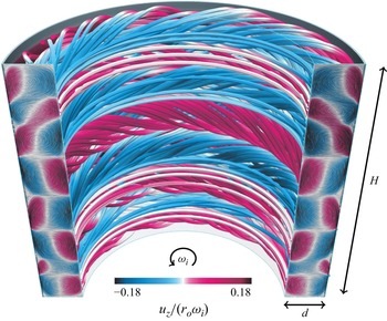


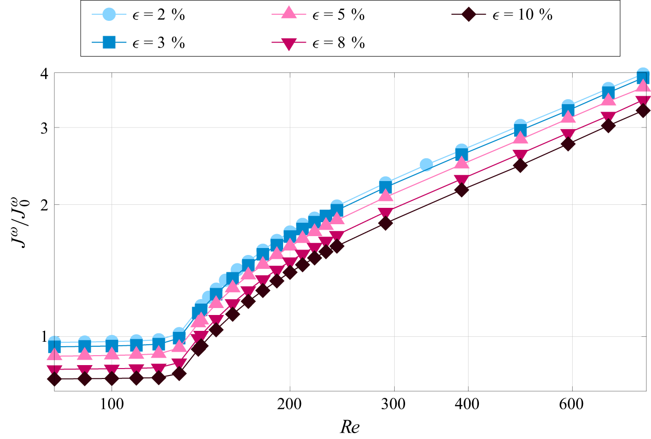


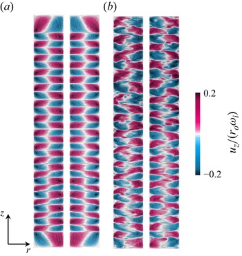


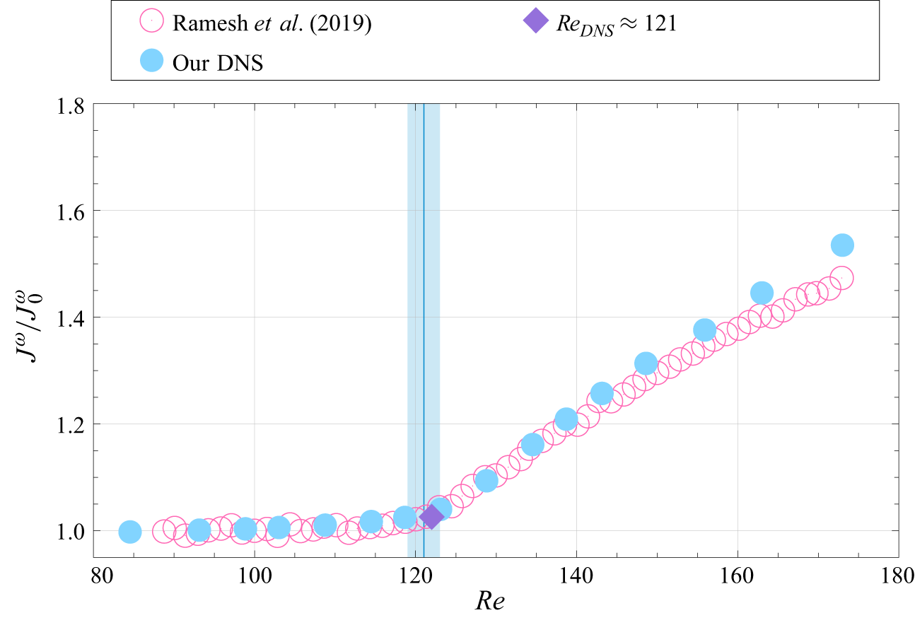


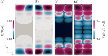


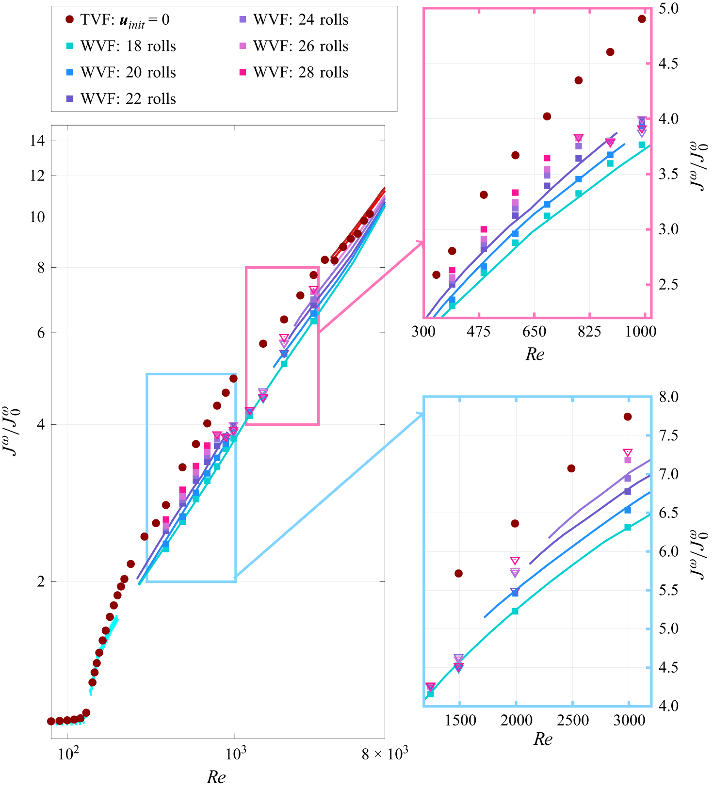


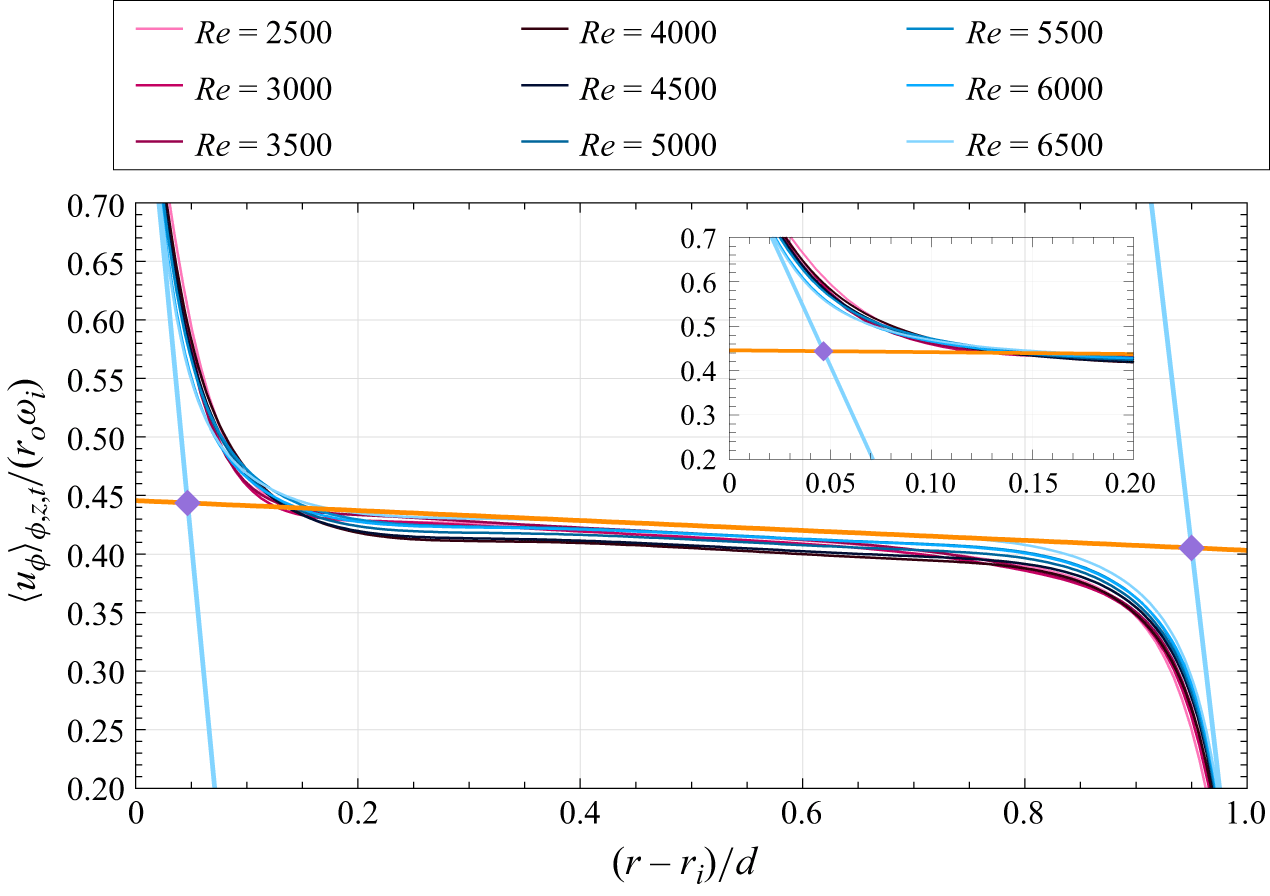


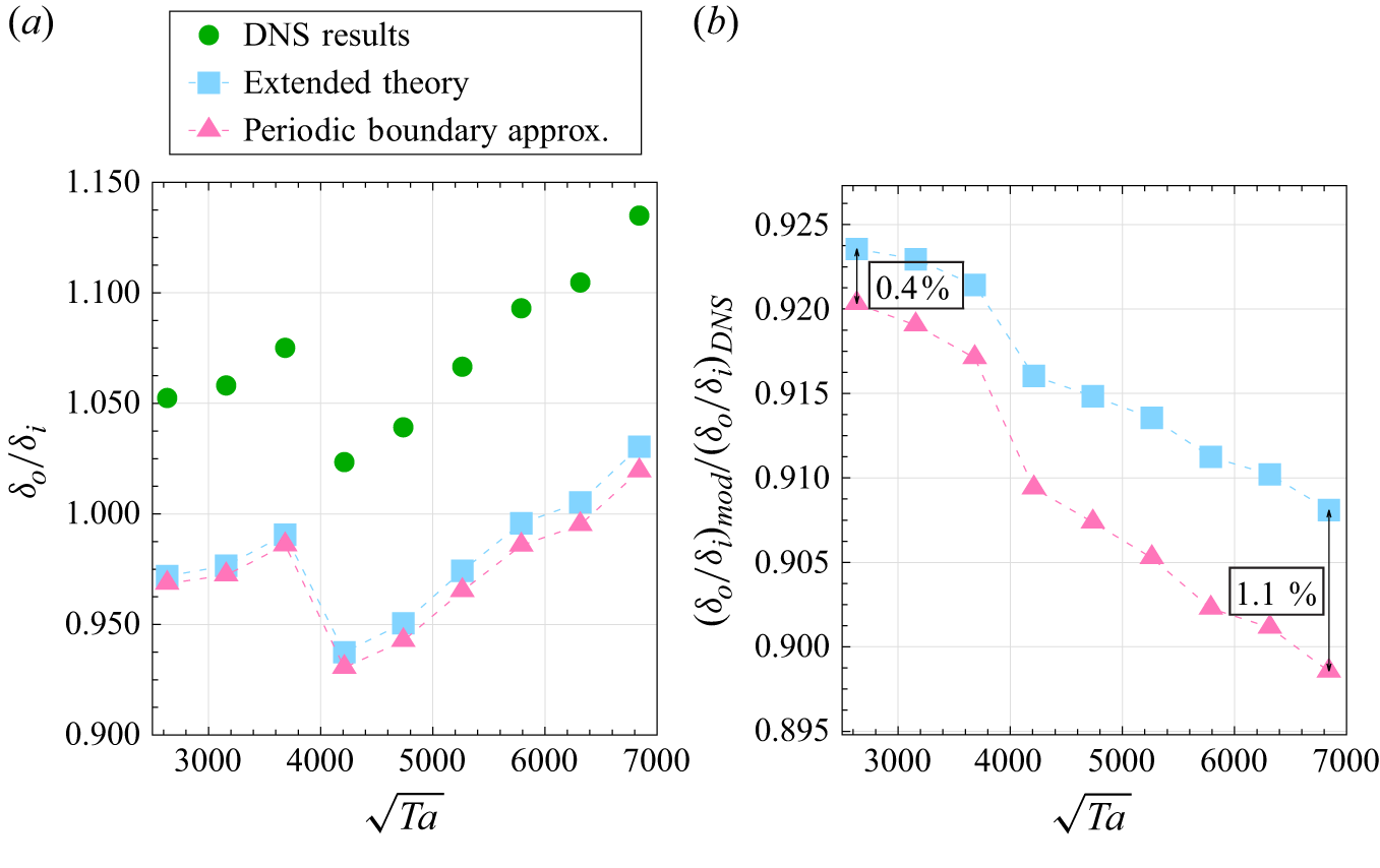


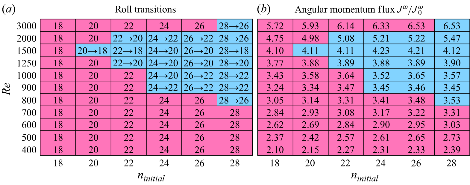


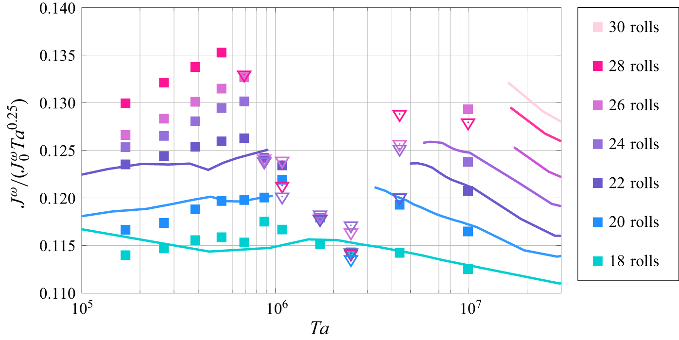


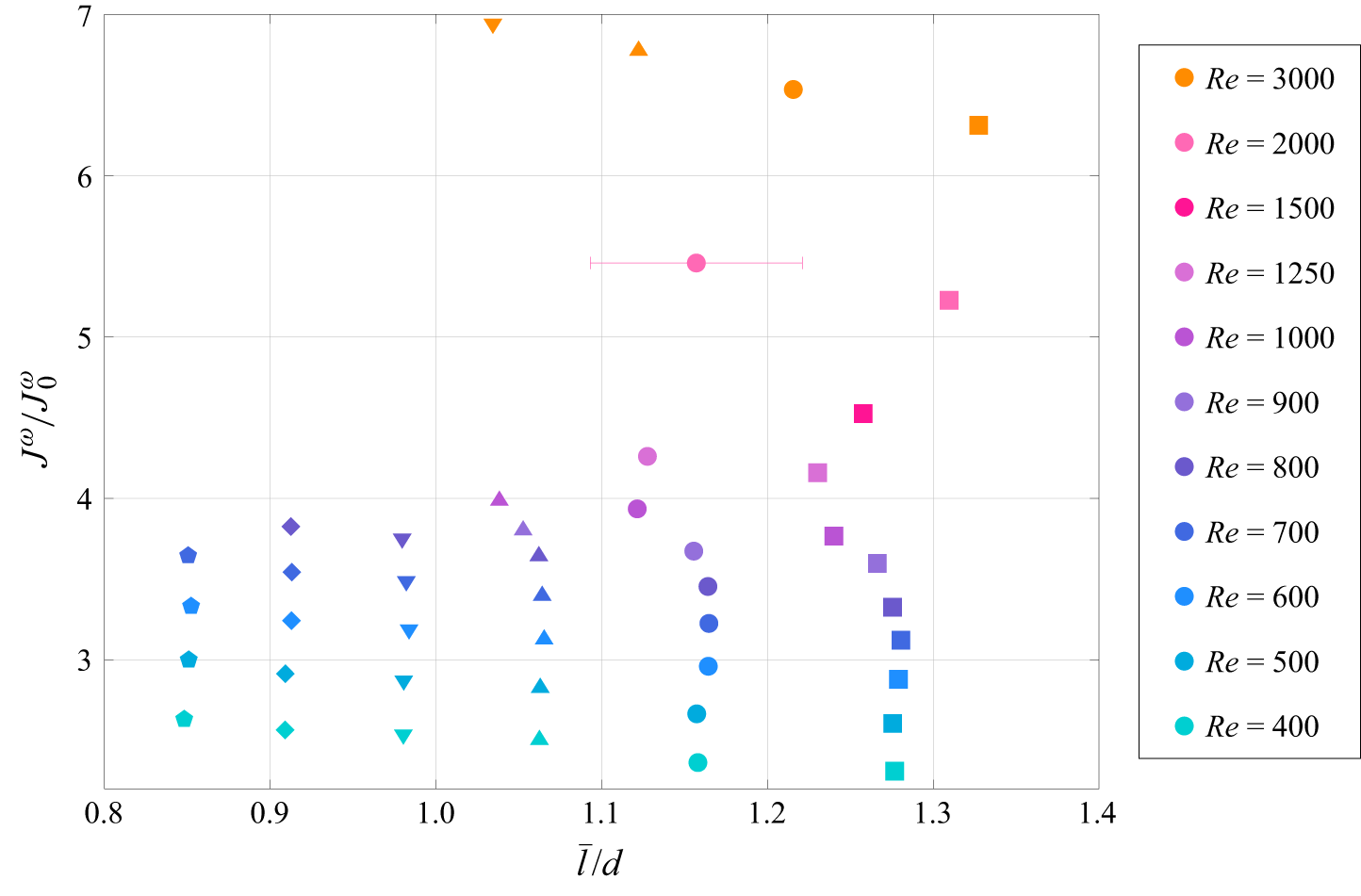


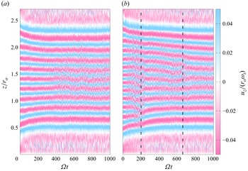


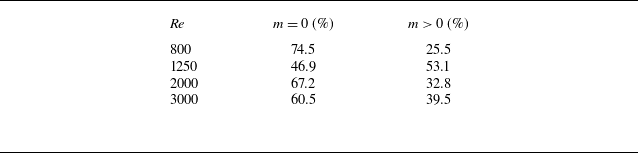
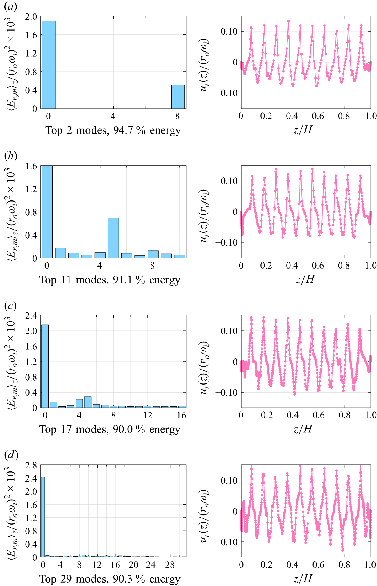


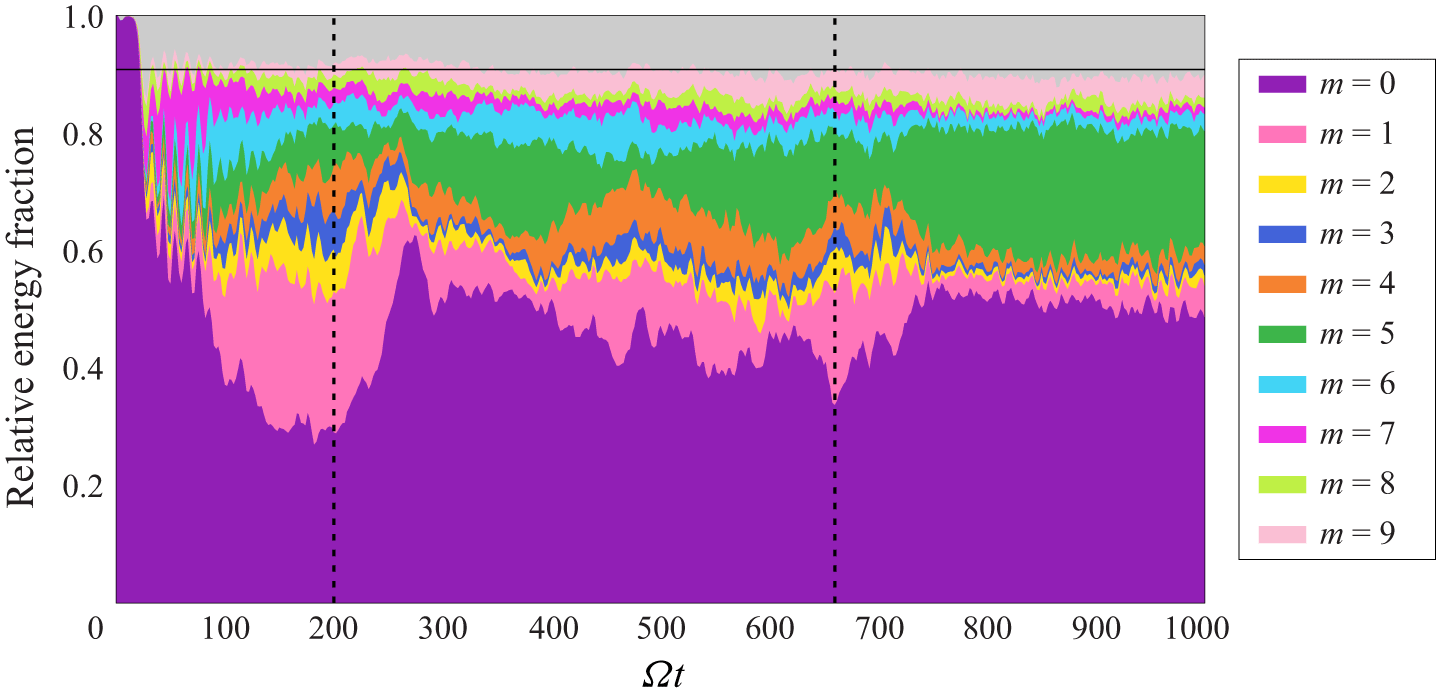


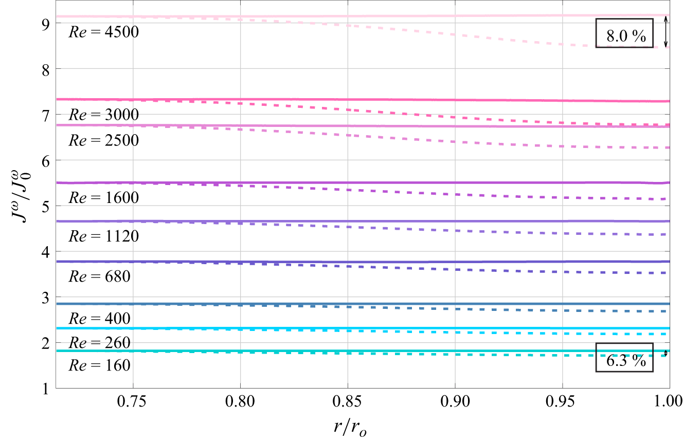


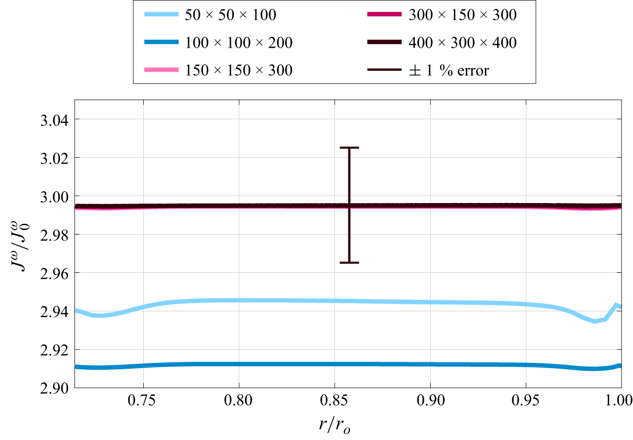


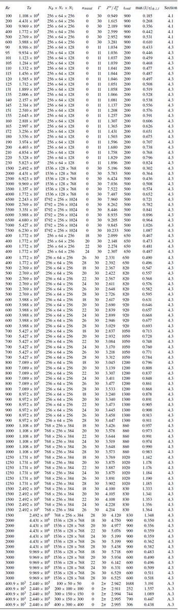


 Open access

